Asymptotic Theory of Elliptic Boundary Value Problems in Singularly Perturbed Domains || Homogenization of Equations on a Fine Periodic Grid

Chapter 20

Homogenization of Equations on a Fine Periodic Grid

Homogenization can be useful not only for studying differential equations but for difference ones, as well. Moreover, to difference equations it was applied even earlier, in the nineteenth century, to analyze the limit passages in discrete models of continua for obtaining continuous ones.

In the present chapter, it is shown how the techniques in Chapter 19 can be modified for constructing asymptotics of solutions to difference equations with rapidly oscillating coefficients on a fine periodic grid. In the first section, we describe the grid, the difference boundary value problem, and the formal procedure of homogenization. The second section is devoted to studying the coefficients of the homogenized system of partial differential equations. We find the ellipticity criterion for the homogenized system and indicate a way to compute its coefficients. In the final third section we apply the above mentioned results to describe a model of crystalline grid and present examples of homogenized operators in the case of hexagonal grids.

In contrast to the preceding chapter, here we do not justify the asymptotics. We do not consider the construction of the complete asymptotic expansions in the interior of the grid and the boundary layer near the rectilinear parts of the boundary. These questions can be studied as in Chapter 19.

20.1 Homogenization of Difference Equations

20.1.1 A grid in IF!.n and the interaction set of its points

Let {Y} be the set of vectors admitting the representation Y = Zldl + ... + zndn, where ZI, ... ,Zn are some integers and d1 , ... ,dn form a basis in IF!.n.

Definition 20.1.1. A set G is defined to be a grid if G is invariant under the shifts by vectors Y E {Y}.

Definition 20.1.2. The elementary cell G of a grid G is defined to be the intersection of G and the parallelepiped with edges d1 , d2 , ... ,dn .

Let the shift of G by a vector Y E {Y} move points t,,, to t', st. For ease of

notation we shall write t" instead of (t, ,,) E G x G.

Definition 20.1.3. A set reG x G i" called the interaction set of the point" of G if for any element "t the set r contains sit' and t's'. The element st E r is called the interaction of s with t.

Let g(s, t) be the set of points 8,81,82, ... ,8p , t such that SSj, S1S2, .. ' ,Sp, t E rand Sj I: Sk for j I: k. If for some s, t there are no points SI, S2,··· ,sp with the mentioned property we put g(s, t) = 0.

283

V. Maz’ya et al., Asymptotic Theory of Elliptic Boundary Value Problems in Singularly Perturbed Domains© Birkhäuser Verlag 2000

284 20. Homogenization of Equations on a Fine Periodic Grid

Definition 20.1.4. A subset C(j) of a grid C is called a subgrid if any sand t in C(j) satisfy g(s, t) =f- 0.

We assume that

C = U C(j). j=1

Definition 20.1.5. A function v on c(j) xr is called G-periodic if for any sand t with interaction st E r and for any s' and t' there holds the equality v(s, st) = v(s', s't').

Let Ce stand for the grid C obtained from C by means of the change of variable x ----) c:-1x with small positive c:. We denote by CY and T the points of Ce corresponding to sand t in C and by x(cy) the Cartesian coordinates of CY E Ce . Suppose that the set 'Y( CY) of points interacting with CY E Ce consists of elements in Ce located at a distance not greater than O(c:) from CY. The set of all interactions of the grid Ce will be denoted by 'Y. We introduce some operators on functions given on Ce or Ce x 'Y.

Definition 20.1.6. Let u be a function given on Ce . The difference operator 8 is defined by the formula

8u(m) = U(T) - u(CY).

Definition 20.1.7. Let v be a function given on Ce X'Y with property v(cy, CYT) = -V(CY, TCY). Then

8*v(CY) = L (V(CY, CYT) + V(T, m)). (1) TE'y(a)

Note that -(v8u)ce nn = (u8*v)ce nn,

n being a domain in jRn with compact closure and smooth boundary 8n. Hereafter (w)Q with Q C Ge stands for

IQI-1 L L w(CY, TCY), aEQ TE'y(a)

where IQI is the number of elements in Q. The same notation (w)Q we shall use for the mean of waver Q C C.

20.1.2 Statement of the problem

We introduce a space S(G) of periodic vector-valued functions v on C x r endowed with the norm

Here M 1/2

Ivl = (L(v(k))2) , k=1

v(k) being the components of v. Let Cm(O; H), mEND, be the space of functions on 0 with values in a Hilbert space H which are continuously differentiable up to order m, and CO = c. We denote by A and B symmetric square matrices of order M with entries ajk(x, ts) and bjk(x, s) given on 0 x rand 0 x G, respectively.

20.1. Homogenization of Difference Equations 285

Suppose that the columns of A and B belong to C 1 (O; S(G)) and C(O; S(G)) while the functions ajk satisfy ajk(x,st) = ajk(x,tS).

In the domain Gc nO we consider the equation

C 28*(A8u) - Bu = f (2)

with f E C (0; S( G)) which is a concise notation for the equality

c-2 L (A(X(T), ts) + A(x(O'), ts)) (U(T) - u(O')) - B(x(O'), s) u(O') TE,),(o-)

Let 8( Gc nO) be the set of points in Gc nO interacting with points in Gc \ O. We assume that the solution u to equation (2) satisfies the boundary condition

(3)

In what follows we study the solvability of problem (2), (3) and find the principal term in the asymptotics of the solution as c ---+ o. 20.1.3 Solvability of the boundary value problem

We introduce a space HO(Gc n 0) of vector-valued functions v on the set Gc nO endowed with the norm

-° - 2 1/2 Ilv;H (Gc nO)11 = (Ivl )oenn '

and a space Hl(Gc n 0) with norm

Ilv; Hl(Gc n 0)11 = (Iv1 2 + c-218vI2)~2nn' The space Hl(Gc n 0) is a Hilbert space with inner product

(VI, V2) = (c- 28 vl . 8V2 + VI' V2)Oe nn ,

where the point denotes the inner product in jRM.

Lemma 20.1.8. There exists the unique solution u E Hl(Gc nO) to equation (2) satisfying (3) and

Ilu; Hl(Gc n 0)11::; c Ilf; fIO(Gc n 0)11· Hereafter c stands for a constant independent of c.

Proof. Any function u equal to zero on 8( Gc nO) satisfies the Friedrichs inequality

(u2)oenn ::; cc-2((8u)2)Oe nn (4)

which can be proved similarly to Proposition 19.2.2. We multiply (2) by TJ E Hl(Gc nO) vanishing on 8(Gc nO). Summing over

0' E Gc no), we obtain

+ L (c-2 L A(X(O'),O'T) 8U(TO')' TJ(O') - B(X(O'),O'T) u(O')' TJ(O')) O'EOen!""! T E-y (0-)

L f(x(O'),s). TJ(O'), uEoe nn


which we rewrite in the form -2 - -

-(c: Aou· OT) + Bu· T})c,no = U' T})cEno)' (5)

Taking account of (4) and the Riesz theorem on the general form of functionals in Hilbert space, we complete the proof. 0

20.1.4 The leading terms in asymptotics

For functions v(x, s) and u(x, ts) in CHI (D; S( G)) there hold the following asymptotic expansions

k

V(X(T), t) - V(X(O'), s) = Dv(x(O'), ts) + L (m!)-1 (l(j)(TO')o/OXj)m v(x(O'), t) m=1

1

+ (k!)-l J (l(j)(TO')O/OXj )k+l v(x(O')(1 - y)

o

+x(T)y,t)(I-y)kdy, k

U(X(T), ts) + u(x(O'), ts) = 2u(x(0'), ts) + L (m!)-1 (l(j)(TO')O/OXj)m u(x(O'), ts) m=l

1

+ (k!)-l J (l(j) (TO')O/OXj) k+1 u(x(O')(1 - y)

o

+x(T)y,ts)(I-y)kdy, kENo. (6)

Here l(k) (TO') are components of the vector l( TO') directed from 0' to T and Dv(x, ts) = v (x, t) - v (x, s). In the sequel we sum over repeating indices from 1 to n.

We apply the operator on the left in (2) to the function v and take (6) into account. Then the result can be written as the formal series

with coefficients

where

Aov = D*(A Dv), Al v = T1 D* (l(j) (o/OXj) A Dv + 2A l(j)ov/oxj)

A2v = 2-1D* {(l( jl%Xj)2 AD v + 2A (l(j) 0/ OXj )2V

+ Z(j)(%xj)A(z(m)ov/oxm)} - Bv,

D*u(x, s) = 2 L v(x, ts) tey( s)

and ,( s) is the set of points interacting with sEC.

(7)

One can seek the asymptotics of the solution to problem (2), (3) in the form

Uo + EU1(X, s) + E2u2(X, s) +... . (8)

Coefficients of the series for k 2: 1 are vector-valued functions periodic in the second variable. Substituting (8) into (7) and equating the coefficients at the same powers of E we obtain the equations for Uk. Since the coefficient at E- 1 vanishes, we have

(9)

20.1. Homogenization of Difference Equations 287

To find U1 we introduce the matrices N(k), k = 1, ... ,n, that are periodic solutions to the equations

D*(ADN(k))(X, s) = -D*(A.l(k))(x, s), k = 1, ... ,n, s E G. (10)

By virtue of (9),

(11) Let us consider the solvability of equations (10) in the class of functions with

G-periodic components.

Lemma 20.1.9. Let the columns of the matrix A. and a vector-valued function F exist in em (G; S( G)) for some m = 0,1, .... The equation

D*(A.Du)(x, s) = F(x, s), x E n, s E G, (12)

is solvable in em (G; S( G)) if and only if

(F)c(x) = O. (13)

A solution u to problem (12) is determined up to a vector constant on every set G(j) = e(j) n G. The constants can be chosen so that

(u)c(j) = 0, j = 1, ... ,x.

The proof can be obtained from the Riesz theorem on a linear functional in Hilbert space and the Poincare inequality

(u2)c::; (u)b + C((Du)2)C' (14)

The estimate (14) follows from the evident relation

U(X,S2) -u(x,sd = L (u(x,t) -u(x,s)), s,tEg(S2,sil

valid for any two points Sl, S2 E G. We square the last equality, sum over S1, S2 E G, apply Cauchy's inequality, and arrive at (14).

Let us turn to the asymptotics of the solution to problem (2), (3). In view of the G-periodicity of ajk and the relations

ajk(x, st) = ajk(x, ts), l(st) = -[(ts),

the right-hand sides of equations (10) satisfy (13). Hence, the equations (10) for N(k) are solvable.

The coefficient U2 in (8) is defined by the equation

AOU2 = -A2UO - A1U1 + f. Its compatibility condition

(J - A2Uo - A1U 1)C = 0

is equivalent to the following equation for uo:

(8/8xj)(A(j,k)(x)(8/8xk)UO(X)) - (.8)c(x)uo(x) = (J)c(x), x E O. (15)

Here A(j,k) is the matrix with entries

A(j,k)(X) = ([(i)[(k) a + [(j) a D N(j))c(x) pq pq pm mq . (16)

In Theorem 20.2.1 below there is a criterion for the strong ellipticity of system (15), which we assume to be fulfilled.


Thus, the coefficient UI in (5) is defined by (11) while Uo satisfies (15) and the boundary condition

uo(x) = 0, x E a~. (17)

(If (17) holds, then the function Uo (x( 0')), 0' E a( Gc nO), is subject to luo (x( 0')) I :::; CE.) The proof of the next assertion is similar to that of Theorem 19.2.4.

Theorem 20.1.10. Let the columns of the matrices A and B are in C3 (O; S(G)) and C I (0; S( G)), respectively, while f E C3 (0; S( G)). Then for the solution u to problem (2), (3) there holds the estimate

Ilu - Uo - CUI; fIl(Gc n 0)11:::; CC1/ 2 ,

where Uo is the solution to problem (15), (17) and Ul is defined by (11).

20.1.5 Asymptotics of the solution to the nonstationary problem

Let u satisfy the equation

R(a/aT)2 u(O', T) - E-2a*(Aau)(0', T) + Bu(O', T) = f(s, x( 0'), T),

0' E Gc no, T E [0, To],

the boundary condition (13) and the initial conditions

u(O', 0) = 0, (a/aT) U(O', 0) = 0, 0' E Gc nO.

(18)

(19)

Here R is a positive definite matrix with entries rjk(x, s) that are G-periodic in the second variable and smooth in x. The entries ajk and bjk of A and B satisfy the assumptions on the coefficients of equation (2) and smoothly depend on T.

The construction ofthe principal term uo(x, T)+CUI (x, s, T) in the asymptotic expansion of the solution to problem (18), (3), and (19) is similar to that of the solution to stationary problem (2), (3) (see Section 20.1.3). The function Uo satisfies the equation

(R)e (a/aT)2 uo(x, T) - (o/OXj) (A(j,k) (x) (O/OXk) uo(x, T)) + (B)e (x) uo(x, T)

= (J)e(x, T), x E 0, T E [0, To],

and the homogeneous initial and boundary conditions. The coefficient Ul is equal to (N(k)O/OXk) Uo, where N(k) is the solution to (10). The justification of the asymptotics follows from the a priori estimate for the solution to problem (18), (3), and (19) and can be carried out according to the scheme in BAKHVALOV and PANASENKO [1].

20.2 Calculation of Coefficients of the Homogenized Operator and Their Properties

Suppose that points of G participate in 2P interactions. To every interaction we associate a number z(st) E {-1,1} such that z(ts) = -z(st).Letp(st) E {1,2, ... ,P} be the index of interaction pairs st and ts (i.e., p(st) = p(ts) but p(st) =I- p(s't') for s't' =I- st and s't' =I- ts). From (10), 20.1, it follows that the matrices N(k) satisfy the equalities

A(x, ts)DN(k) (x, ts) = -Z(k)(ts)A(x, ts) + z(ts)C(k,P(ts)) (x), s E G, t E ,(s), (1)

20.2. Calculation of Coefficients and Their Properties 289

with matrices C(k,p) subject to

L z(ts)C(k,P(ts)) (x) = 0, s E G, k = 1, ... ,n. (2) tE"/(s)

Using (1), we write coefficients of the homogenized operator in the form

A~qk)(x) = [G[-l L L z(ts)z(j) (ts)CidP(ts)) (x). (3) aEGtE,,/(s)

To check ellipticity of the homogenized operator and calculate its coefficients, we describe the construction of the matrices C(k,p). Let us connect the interacting points of the grid {; by straight lines. We denote by K the set of points where these lines meet the faces of the parallelepiped Q with edges d1 , d2 , ... ,dn (see Section 20.1.1). If t E K, then t* stands for the point symmetric with respect to the plane passing through the center of Q and parallel to the face of Q that contains t. Owing to the periodicity of r, the point t* is in K. We identify the points t and t*. Then the lines connecting the interacting points form the graph Y with P edges and 8 nodes, which are elements of G.

The graph Y has x connected components. From (1) and the G-periodicity of A and N(k) it follows that (zC(k,p))G(J) (x) = 0, j = 1, ... ,x, k = 1, ... ,n. Therefore, the relations (2) are linearly dependent. We exclude x linearly dependent equations and obtain 8 - x equations for the matrices C(k,p). It is known (e.g., see ZYKOV [1], Chapter 3) that a graph with P edges, 8 vertices, and x connected components has P - 8 + x independent cycles. Denote linear independent cycles of the graph Y by Yq, q = 1,2, ... ,P - 8 + x. By (1), for any two interacting points sand t of the set G there holds the relation

N(k)(x, t) = N(k)(x, s) _Z(k)(ts) E + z(tS)A-l(X, ts)C(k,P(ts)) (x), k = 1, ... ,n, (4)

E being the identity M x M matrix. Summing up (4) over all edges of the cycle Yq, we have

L z(ts)A-l(x, ts)C(k,P(ts)) (x) = L Z(k) (ts) E, k = 1, ... ,n. (5)

Thus, nM2 P functions C~':;.p) are given by (2) and (5). If the matrices C~k,p) satisfy (2), (5), then the corresponding functions N~k) can be obtained from the equations

(k) (k) - 1 (k,p(ts)) DNo (x, ts) = -Z (ts) E + A- (x, ts) z(ts) Co (x),

s E G, t E /,(s), k = 1, ... ,n, (6)

while the conditions (5) are necessary and sufficient for the solvability of system

(6). Using (1), one can find C~k,p). Therefore, the unique solvability of the system of equations for C(k,p) follows from that of system (10), 20.1. We rewrite the system (2), (5) for N(k) in the form

iJe = W. (7)

Here e is a matrix consisting of P x n blocks of size M x M. The q-th block of the k-th column of blocks consists of the functions C~/). The PM x PM matrix iJ consists of blocks of size M x M. The first 8 - x rows of blocks in B correspond to


the points of the set G, where are given the linear independent equations (2). If the equation (2) corresponding to the k-th row (k < 8 - x) contains the matrix ±C(j,p) ,

then the p-th element of the k-th row is ±E, otherwise the p-th element is equal to the zero matrix. The next P - 8 + x rows of blocks of the matrix B correspond to the independent cycles of Y which are subject to (6). If the interaction st with index p(st) is involved in the k-th cycle, then the p-th position in the (k - 8 + x)-th row (p = p( st)) is taken by the matrix z (st) A -1 (x, st) otherwise the matrix is replaced by the zero matrix. Finally, the matrix W contains P x n blocks of size M x M. In the first 8 - x rows the blocks consists of zeros. The q-th position of the k-th row of blocks with k > 8 - x is taken by the matrix

L l(q)E.

raEYk- 8+x

The ellipticity criterion for the homogenized operator A is related to the structure ofW.

Theorem 20.2.1. The inequality

M

'" A(j,k)c(m)c(i) > 0 L m, "J "k

rn,i=l

(8)

holds for any vectors ~j E ]RM, ~j -I 0, j = 1, ... ,n, if and only if the rank of W is equal to nM.

Proof. We change the order of summation, take account of (10), 20.1, and of the G-periodicity of the entries of the matrices A and N(k) and obtain

M M

L (l(k)armDN;;'~/c = - L (N;;'~D*(arml(k))/c m=l m=l

M M

- '" (N(j)D*( 'DN(k))\ - - '" ( ·DN(k)DN(j)) - L mq art im /c - L art im mq c· m,i=l m,i=l

(9) From (9) it follows that

M

A~~k)(x) = L (ari(8im l(j) + DNi~))(8mq l(k) + DN;;J)/c. m,i=l

Therefore, according to (1),

A~~k)(x) = 8- 1 L L t CrV,P(tS)) (x) him(x, ts) C~~P(tS)) (x), sEC tE'y(s) m,i=l

him being the elements of A-I. From this we derive that for any vectors ~j E ]RM, ~j -I 0, j = 1, ... ,n, there holds the formula

M

L A~ik)(x)~3m)~ki) m,i=l

~ '" '" C(j,P(tS))( )h. ( t ) C(k,P(ts))c(r)c(q) L L L n x ,m x, S mq "J "k .

r,m,i,q=l sEC tE,ls)

20.3. Crystalline Grid 291

Since the matrix A -1 is positive definite, we have

t A~ik)(x)~t)di) ~ L L t (C~~p(ts)) (x)~]m)( (10) m,i=1 sEG tey(s) q,m=1

Suppose that the rank of W equals nM. The system of equations for C~{,p) is

uniquely solvable and the matrix 13 is nonsingular. Hence, the rank of 6 is equal to that of W so some terms on the right in (10) differ from zero, i.e., the inequality (8) is fulfilled.

N ow we assume that the rank of Wand, consequently, the rank of 6 is less than nM. Then there exist numbers O:mq such that

M

"" 0: C(j,p) = 0 ~ mq mq m=1

for all p = 1, ... ,P, q = 1, ... ,M. By virtue of (3),

:=: = t A~ik)~]m)di) = 8-1 L L t z(ts)l(j)(ts)Ci~p(tS)) (x)~t\iq)· m,i=1 sEG tey(s) m,q=1

Choosing d q) = O:kq, we obtain :=: = 0 so (8) cannot be fulfilled.

20.3 Crystalline Grid

20.3.1 Equations of the elasticity theory

D

In the case of M = n = 2 or M = n = 3 one can apply the relation (2), 20.1, to describe the interaction of atoms in a crystalline grid. For instance, in MOROZOV

[3] and NAZAROV and PAUKSHTO [1] the interaction of atoms in a plane is modelled by means of a system of bars with longitudinal rigidity K and transverse one L. According to MOROZOV [3] and NAZAROV and PAUKSHTO [1], the elements of the matrix A are of the form

ajk(ts) = K(ts) w(j) (ts)w(k) (ts) + L(ts)(8jk - w(j)(ts)w(k)(ts)), (1)

w(k) being the projection onto the axis Xk of the unit vector directed from s to t. In view of the relation

A~. ~ = (~(i)w(i))2 K + {~(i)~(i) _ (~(k)w(k))2}L

= (~(i)w(i))2 K + {~(m) _ (~(j)w(j))w(m)}{~(m) _ (~(k)w(k))w(m)}L,

the matrix A is positive definite. Construction of asymptotics of the solution to problem (2), (3), 20.1, iIllplelIlent~ the limit pa~~age from the equation of the crystalline grid to the equations of solid bodies. The elasticity theory equations

(O/OXk)(Aikjm(X)(O/oXj)u(m)(x)) = f(i) (x) (2)

are symmetric and elliptic. We show that the same is true for equation (15), 20.1, which provides the principal term in asymptotics of the solution to problem (2), (3), 20.1.

Theorem 20.3.1. In the case of a crystalline grid the homogenized operator A is the operator of elasticity theory.


Proof. Under the assumptions of Theorem 20.2.1, the operator A of equation (15), 20.1, is elliptic. Let us check that its coefficients satisfy the symmetry relations corresponding to the symmetry of Aikjm:

A(j,k) = A(k,j) (3) pq pq' A(j,k) = A(p,q) (4)

pq Jk

We prove (3). If a G-periodic function f satisfies f(st) = f(ts), then

L L f(ts)h(s) = L L f(ts)h(s), (5) sEOtE'y(s) tEO SE'y(t)

h being a G-periodic function on the set G. By virtue of (10), 20.1,

""' (i) _ ""' (i) ~ apm(x, ts) DNmq(x, ts) - - ~ apq(x, ts) Z (ts). (6) tE,(s) tE,(s)

We multiply (6) by Z(k) (rs) for i = j and by Z(j)(rs) for i = k, sum over s E G, take (5) into account, and arrive at

L L (Z(k) (rs) apm(x, ts) DN~6(x, ts)) tEO sE,(t)

= L L (l(j)(rs) apm(x,ts) DN::J(x,ts)), rEG. (7)

tEO sE,(t)

Setting r = t, we obtain (3). Let us verify (4). Since the inner state of a crystalline grid does not depend

on rotations, for any point s E G

L (z(j) (ts) apq(x, ts)) = L (Z(q) (rs) apj(x, ts)), (8) tE,( s) tE,( s)

(e.g., see KOSEVITCH [1]). We multiply (8) by Z(k)(rs) and sum over s E G. By virtue of (5), there holds the identity

L L (l(j)(ts) Z(k) (rs) apq(x, ts)) tEO sE,(t)

= L L (z(q) (ts) Z(k) (rs) apj(x, ts)), rEG. tEO sE,(t)

(9)

Setting j = k,p = j, q = p, k = q in (9) and adding (9), we conclude that for r = t

(Z(j) Z(k)apq)o = (Z(q) Z(P)ajk)o, (10)

We multiply (7) by Z(p) (rt) for i = q, p = j, q = k and by Z(k) (rt) for i = j. Now we sum over s E G, make use of (6), and set r = t. Taking (10) into account, we obtain

(11)

The formula (4) follows from (10), (11), and the definition of the coefficients of A. Thus, (15), 20.1, is the equation of elasticity theory. D


20.3.2 Examples of homogenized operators

A grid whose cells consist of one element is called simple. In the case of a simple grid the relation A(x, ts)l(j) (ts) = -A(x,st)l(j)(st) and equation (10), 20.1, imply that all elements of the matrix N(j), j = 1, ... ,n, vanish. Hence, the coefficients of the operator A satisfy

AV/)(x) = (l(j) l(k)apq)c(x). (12)

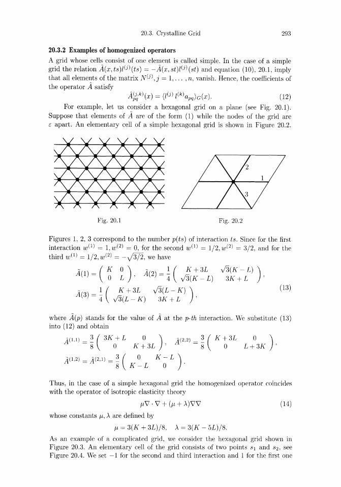
For example, let us consider a hexagonal grid on a plane (see Fig. 20.1). Suppose that elements of A are of the form (1) while the nodes of the grid are E apart. An elementary cell of a simple hexagonal grid is shown in Figure 20.2.

Fig. 20.1 Fig. 20.2

Figures 1, 2, 3 correspond to the number p(ts) of interaction ts. Since for the first interaction w(l) = 1, w(2) = 0, for the second W(l) = 1/2, W(2) = 3/2, and for the third w(1) = 1/2,w(2) = -J372, we have

- (K 0) - 1 ( K + 3L A(l) = 0 L ' A(2) = 4 v'3(K - L)

v'3(K-L) ) 3K+L '

A(3) = ! ( K + 3L J3(L - K) ) 4 v'3(L - K) 3K + L '

(13)

where A(p) stands for the value of A at the ~th interaction. We substitute (13) into (12) and obtain

A(l,l) = ~ ( 3K + L 0 ) j(2,2) = ~ ( K + 3L 0 ) 8 0 K + 3L' 8 0 L + 3K '

j(1,2) = j(2,1) = ~ ( 0 K - L ) . 8 K -L 0

Thus, in the case of a simple hexagonal grid the homogenized operator coincides with the operator of isotropic elasticity theory

/1\7 . \7 + (/1 + >')\7\7

whose constants /1, >. are defined by

/1 = 3(K + 3L)/8, >. = 3(K - 5L)/8.

(14)

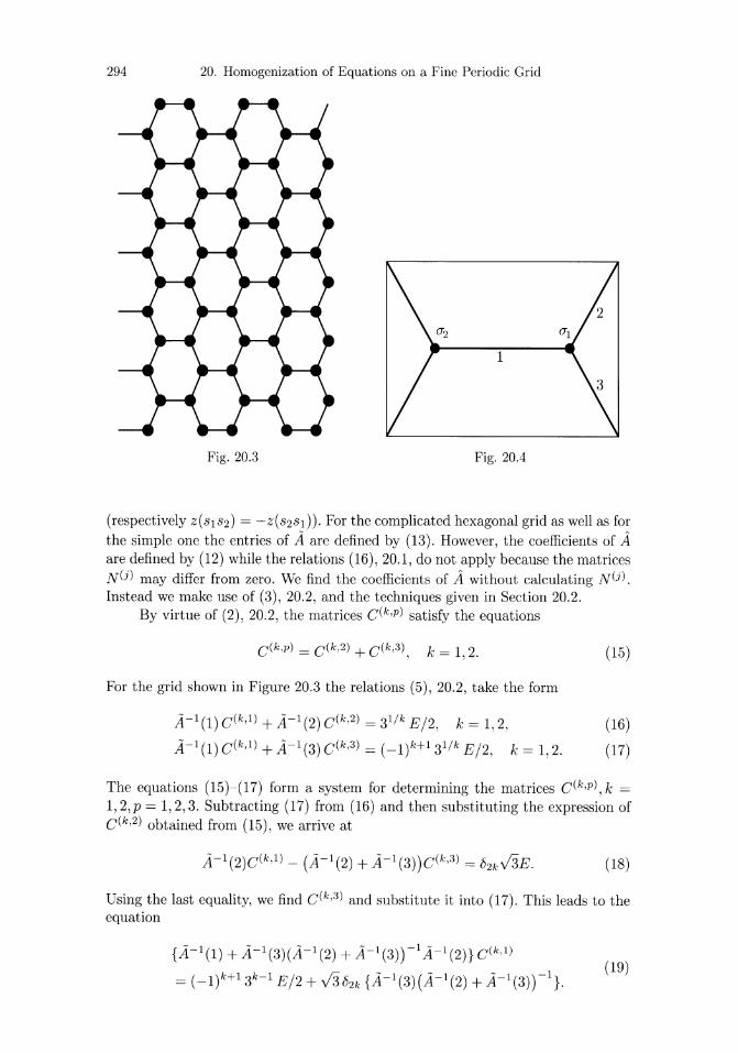
As an example of a complicated grid, we consider the hexagonal grid shown in Figure 20.3. An elementary cell of the grid consists of two points Sl and S2, see Figure 20.4. We set -1 for the second and third interaction and 1 for the first one


1

Fig. 20.3 Fig. 20.4

(respectively Z(SlS2) = -Z(S2SI)). For the complicated hexagonal grid as well as for the simple one the entries of A are defined by (13). However, the coefficients of A are defined by (12) while the relations (16), 20.1, do not apply because the matrices NUl may differ from zero. We find the coefficients of A without calculating N(j).

Instead we make use of (3), 20.2, and the techniques given in Section 20.2. By virtue of (2), 20.2, the matrices C(k,p) satisfy the equations

C(k,p) = C(k,2) + C(k,3), k = 1,2. (15)

For the grid shown in Figure 20.3 the relations (5), 20.2, take the form

A-l(l) C(k,l) + A-l(2) C(k,2) = 31/ k E/2, k = 1,2, (16)

A-l(l)C(k,l) +A-l(3)C(k,3) = (_1)k+l31/ k E/2, k = 1,2. (17)

The equations (15)-(17) form a system for determining the matrices C(k,p), k = 1, 2,p = 1,2,3. Subtracting (17) from (16) and then substituting the expression of C(k,2) obtained from (15), we arrive at

Using the last equality, we find C(k,3) and substitute it into (17). This leads to the equation

{A-l(l) + A-1(3)(A-1(2) + A-1(3)) -1 A-1(2)} C(k,l)

= (_1)k+l3k- 1 E/2 + v'382k {A-l(3)(A-l(2) + A-l(3)) -I}. (19)


The matrices in the braces on the left and on the right in (19) are respectively equal to

(r"(3K :L)f' ),

(K + 3L)-1J3(k - L) ) 1 .

Therefore, from (19) it follows that

C(1,I) = (2(K + L))-1 ( (3L + K)K 0 ) o (3K + L)L '

C(2,1) = (2(K + L)r1(K - L) (~ ~).

Taking (18) into account we obtain

C(1,3) = (4(K L)) -1 ( K(3L + K) J3L(L - K) ) + J3K(L - K) L(3K + L) ,

C(2,3) = (4(K L))-1 ( -J3L(3K + L)K K(K - L) ) + L(L - K) J3K(3L - K) .

From (15), (20), and (21) we derive that

C(1,2) = (4(K L))-1 ( K(3L + K) + J3K(K - L)

C(2,2) = (4(K + L)r1 ( J3L(3K + L) L(K - L)

J3L(K - L) ) L(3K+L) ,

K(K - L) ) J3K(3L+ K) .

(20)

(21)

(22)

Thus, formulas (20)-(22) provide the solution to the system (15)-(17). We substitute the expressions obtained into (3), 20.2, and compute the matrices A(j,m):

;1(1,1) = 3(4(K + L))-1 ( K(3Lo+ K) 0 ) L(3K + L) ,

A(2,2) = 3(4(K + L))-1 ( L(3KO+ L) 0 ) K(3L + K) ,

A(I,2) = 3(4(K + L))-1 ( 0 K(K - L) ) L(K-L) 0 '

;1(2,1) = 3(4(K + L)r 1 ( K(KO _ L) L(KO- L) ) .

In the case of the hexagonal grid shown in Figure 20.3, the homogenized operator coincides with the operator (14) of isotropic elasticity theory where

f.L = (4(K + L)r 1 3L(L + 3K) and A = (4(K + L)r13(K2 - 3LK - 2L2)

are Lame's coefficients.

Documents

Asymptotic Theory of Elliptic Boundary Value Problems in Singularly Perturbed Domains || Homogenization of Equations on a Fine Periodic Grid