Embed Size (px)
Citation preview
© Fraunhofer IDMT
Audio CodingQuantization and Coding Methods Prof. Dr.-Ing. Karlheinz Brandenburg
© Fraunhofer IDMT
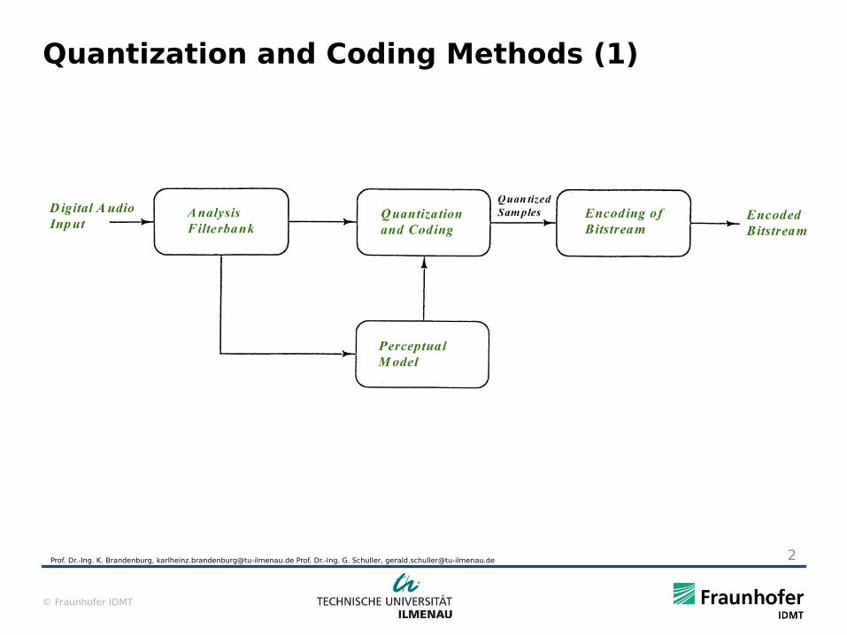
Quantization and Coding Methods (1)
Prof. Dr.-Ing. K. Brandenburg, [email protected] Prof. Dr.-Ing. G. Schuller, [email protected] 2
© Fraunhofer IDMT
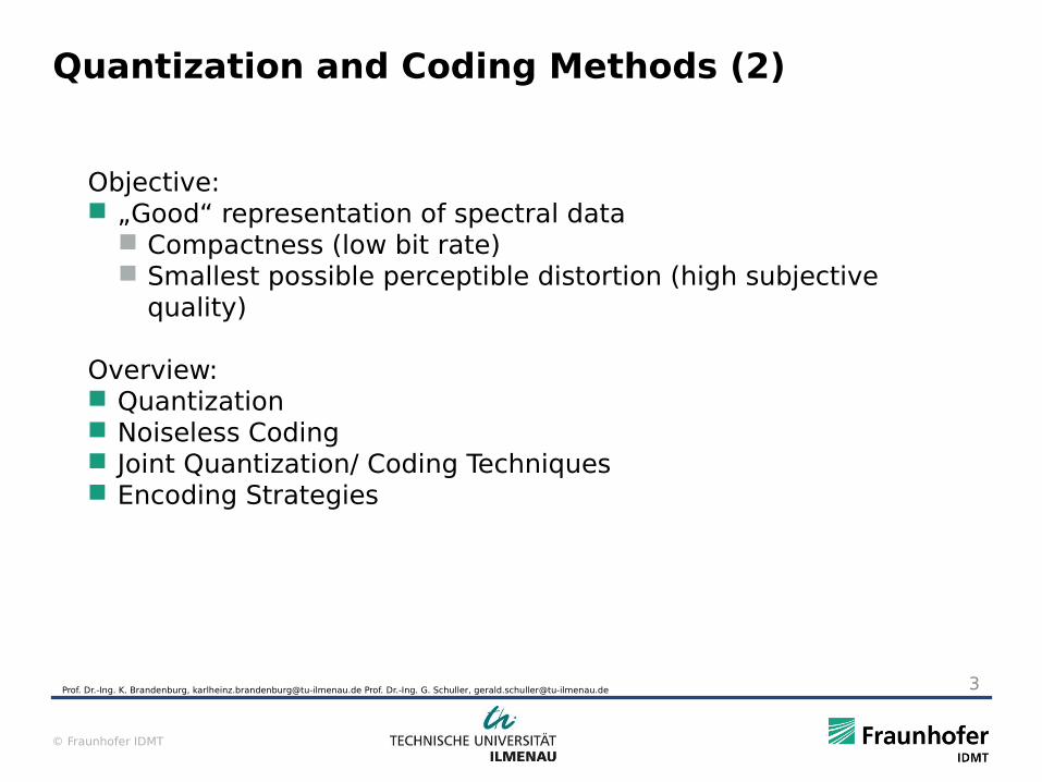
Quantization and Coding Methods (2)
Objective: „Good“ representation of spectral data
Compactness (low bit rate) Smallest possible perceptible distortion (high subjective
quality)
Overview: Quantization Noiseless Coding Joint Quantization/ Coding Techniques Encoding Strategies
Prof. Dr.-Ing. K. Brandenburg, [email protected] Prof. Dr.-Ing. G. Schuller, [email protected] 3
© Fraunhofer IDMT
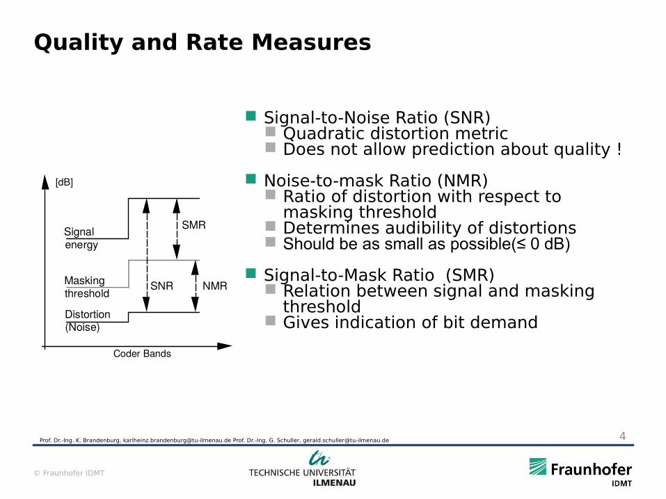
Quality and Rate Measures
Signal-to-Noise Ratio (SNR) Quadratic distortion metric Does not allow prediction about quality !
Noise-to-mask Ratio (NMR) Ratio of distortion with respect to
masking threshold Determines audibility of distortions Should be as small as possible(≤ 0 dB)
Signal-to-Mask Ratio (SMR) Relation between signal and masking
threshold Gives indication of bit demand
Coder Bands
[dB]
Signalenergy
Maskingthreshold
Distortion(Noise)
SNR
SMR
NMR
Prof. Dr.-Ing. K. Brandenburg, [email protected] Prof. Dr.-Ing. G. Schuller, [email protected] 4
© Fraunhofer IDMT
Quantization (1)
Basics: Data reduction by removing irrelevance Explicit control of quantization distortion according to
time/frequency-dependent masking threshold (perceptual coder)
High variability in local SNR (e.g. 0db ... >30db)
Most popular case: Scalar quantization
Prof. Dr.-Ing. K. Brandenburg, [email protected] Prof. Dr.-Ing. G. Schuller, [email protected] 5
© Fraunhofer IDMT
Quantization (2)
x
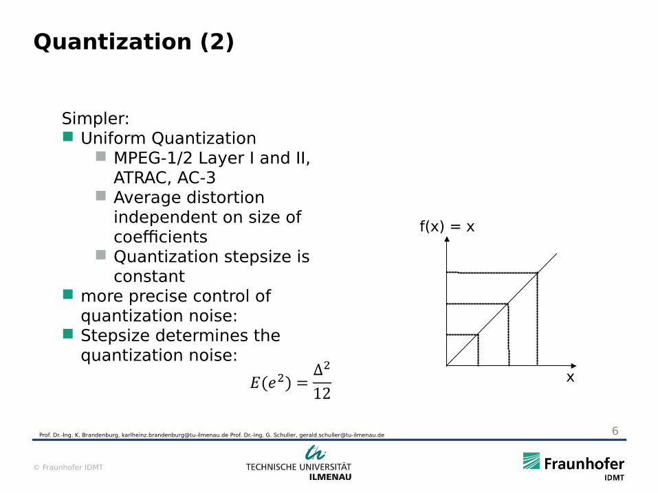
f(x) = x
Simpler: Uniform Quantization
MPEG-1/2 Layer I and II, ATRAC, AC-3
Average distortion independent on size of coefficients
Quantization stepsize is constant
more precise control of quantization noise:
Stepsize determines the quantization noise:
Prof. Dr.-Ing. K. Brandenburg, [email protected] Prof. Dr.-Ing. G. Schuller, [email protected] 6
© Fraunhofer IDMT
Quantization (3)
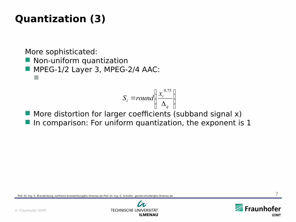
More sophisticated: Non-uniform quantization MPEG-1/2 Layer 3, MPEG-2/4 AAC:
More distortion for larger coefficients (subband signal x) In comparison: For uniform quantization, the exponent is 1
Prof. Dr.-Ing. K. Brandenburg, [email protected] Prof. Dr.-Ing. G. Schuller, [email protected] 7
q
ii
xroundS
75.0
© Fraunhofer IDMT
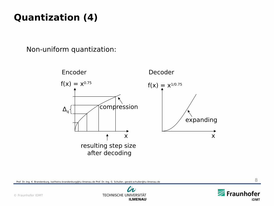
x
Δq
f(x) = x0.75
Encoder
compression
resulting step size after decoding
Quantization (4)
x
f(x) = x1/0.75
Decoder
expanding
Non-uniform quantization:
Prof. Dr.-Ing. K. Brandenburg, [email protected] Prof. Dr.-Ing. G. Schuller, [email protected] 8
© Fraunhofer IDMT
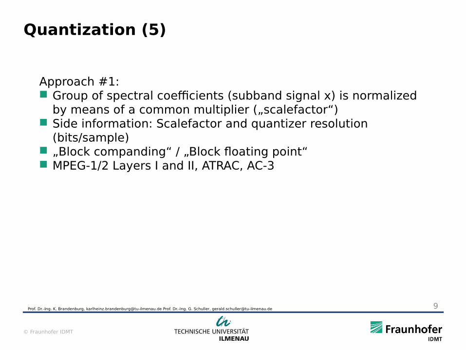
Quantization (5)
Approach #1: Group of spectral coefficients (subband signal x) is normalized
by means of a common multiplier („scalefactor“) Side information: Scalefactor and quantizer resolution
(bits/sample) „Block companding“ / „Block floating point“ MPEG-1/2 Layers I and II, ATRAC, AC-3
Prof. Dr.-Ing. K. Brandenburg, [email protected] Prof. Dr.-Ing. G. Schuller, [email protected] 9
© Fraunhofer IDMT
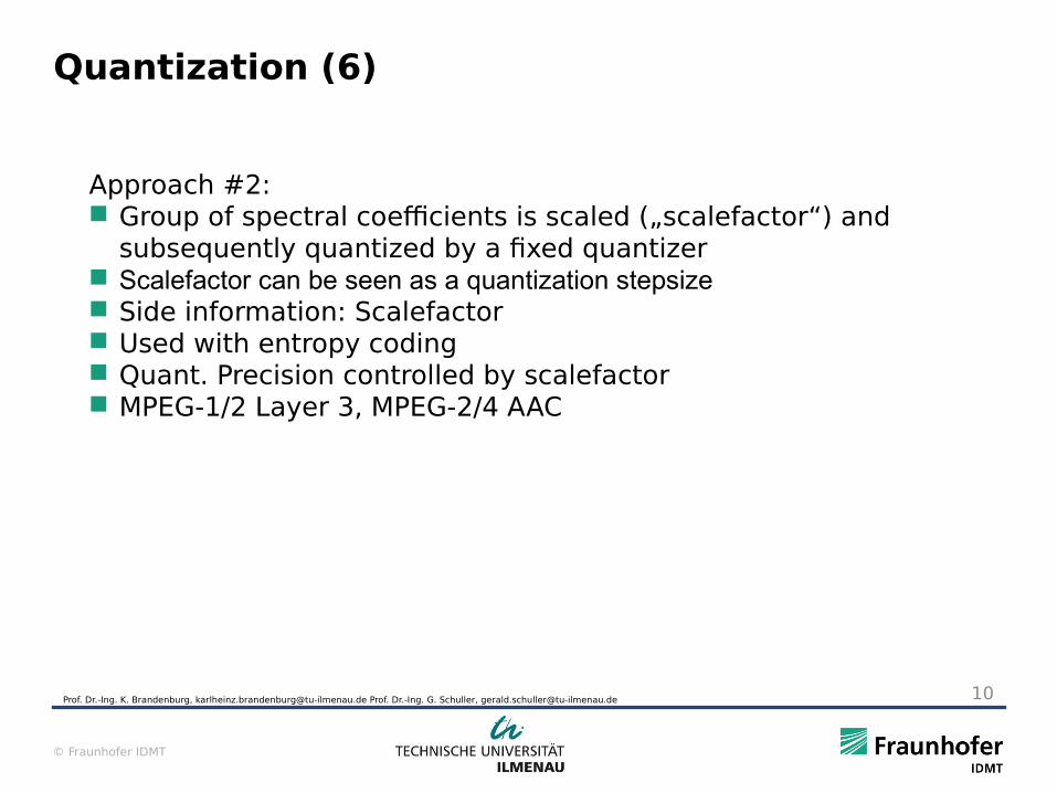
Quantization (6)
Approach #2: Group of spectral coefficients is scaled („scalefactor“) and
subsequently quantized by a fixed quantizer Scalefactor can be seen as a quantization stepsize Side information: Scalefactor Used with entropy coding Quant. Precision controlled by scalefactor MPEG-1/2 Layer 3, MPEG-2/4 AAC
Prof. Dr.-Ing. K. Brandenburg, [email protected] Prof. Dr.-Ing. G. Schuller, [email protected] 10
© Fraunhofer IDMT
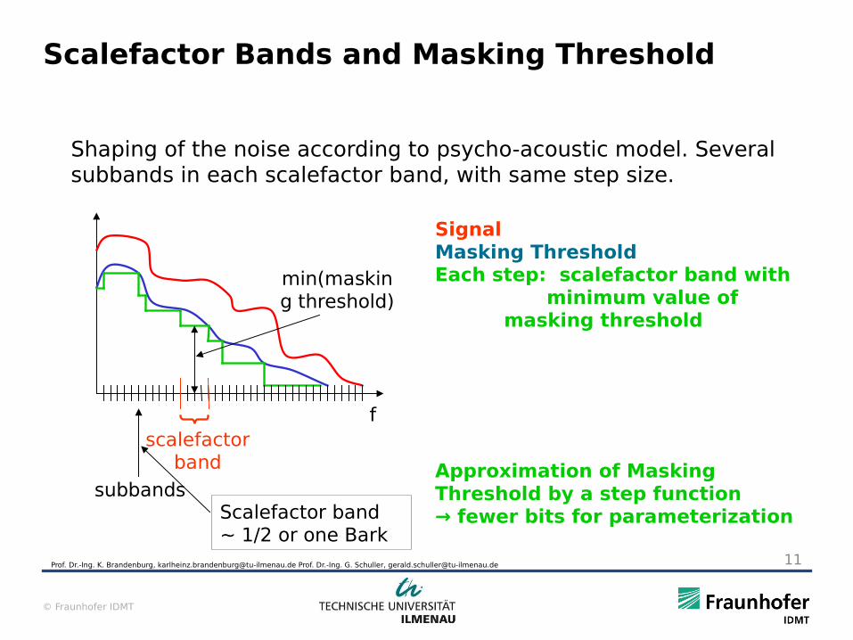
Shaping of the noise according to psycho-acoustic model. Several subbands in each scalefactor band, with same step size.
SignalMasking ThresholdEach step: scalefactor band with
minimum value of masking threshold
Approximation of Masking Threshold by a step function → fewer bits for parameterization
fscalefactor
band
subbands
min(masking threshold)
Scalefactor Bands and Masking Threshold
Prof. Dr.-Ing. K. Brandenburg, [email protected] Prof. Dr.-Ing. G. Schuller, [email protected] 11
Scalefactor band~ 1/2 or one Bark
© Fraunhofer IDMT
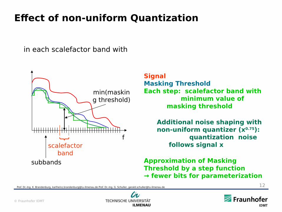
Effect of non-uniform Quantization
in each scalefactor band with
SignalMasking ThresholdEach step: scalefactor band with
minimum value of masking threshold
Additional noise shaping with non-uniform quantizer (x0.75): quantization noise
follows signal x
Approximation of Masking Threshold by a step function → fewer bits for parameterization
fscalefactor
band
subbands
Prof. Dr.-Ing. K. Brandenburg, [email protected] Prof. Dr.-Ing. G. Schuller, [email protected] 12
min(masking threshold)
© Fraunhofer IDMT
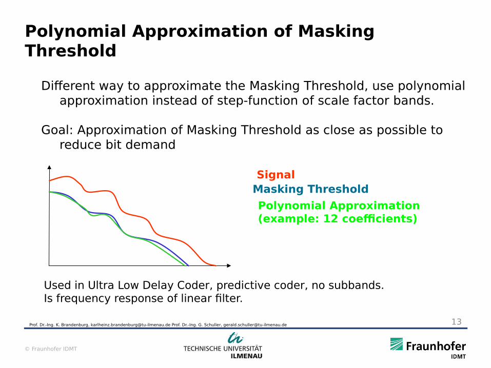
Different way to approximate the Masking Threshold, use polynomial approximation instead of step-function of scale factor bands.
Goal: Approximation of Masking Threshold as close as possible to reduce bit demand
Used in Ultra Low Delay Coder, predictive coder, no subbands.Is frequency response of linear filter.
SignalMasking Threshold
Polynomial Approximation (example: 12 coefficients)
Polynomial Approximation of Masking Threshold
Prof. Dr.-Ing. K. Brandenburg, [email protected] Prof. Dr.-Ing. G. Schuller, [email protected] 13
© Fraunhofer IDMT
MDCT subbands which fall into one scalefactor band their power sums up
Conversion of DFT/MDCT frequency bands into 1/2 or one Bark, at low frequencies broader
After quantization more efficient representation of the codewords is needed noiseless coding
Scalefactor bands
Prof. Dr.-Ing. K. Brandenburg, [email protected] Prof. Dr.-Ing. G. Schuller, [email protected] 14
© Fraunhofer IDMT
Noiseless Coding (1)
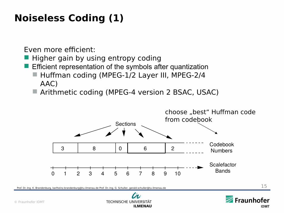
Even more efficient: Higher gain by using entropy coding Efficient representation of the symbols after quantization
Huffman coding (MPEG-1/2 Layer III, MPEG-2/4 AAC)
Arithmetic coding (MPEG-4 version 2 BSAC, USAC)
ScalefactorBands
3CodebookNumbers8 0 6 2
Sections
0 1 2 3 4 5 6 7 8 9 10
choose „best“ Huffman code from codebook
Prof. Dr.-Ing. K. Brandenburg, [email protected] Prof. Dr.-Ing. G. Schuller, [email protected] 15
© Fraunhofer IDMT
Noiseless Coding (2)
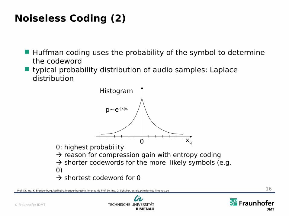
00: highest probability reason for compression gain with entropy coding shorter codewords for the more likely symbols (e.g. 0) shortest codeword for 0
Histogram
xq
p~e-|x|/c
Huffman coding uses the probability of the symbol to determine the codeword
typical probability distribution of audio samples: Laplace distribution
Prof. Dr.-Ing. K. Brandenburg, [email protected] Prof. Dr.-Ing. G. Schuller, [email protected] 16
© Fraunhofer IDMT
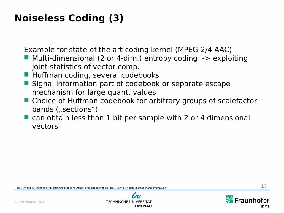
Noiseless Coding (3)
Example for state-of-the art coding kernel (MPEG-2/4 AAC) Multi-dimensional (2 or 4-dim.) entropy coding -> exploiting
joint statistics of vector comp. Huffman coding, several codebooks Signal information part of codebook or separate escape
mechanism for large quant. values Choice of Huffman codebook for arbitrary groups of scalefactor
bands („sections“) can obtain less than 1 bit per sample with 2 or 4 dimensional
vectors
Prof. Dr.-Ing. K. Brandenburg, [email protected] Prof. Dr.-Ing. G. Schuller, [email protected] 17
© Fraunhofer IDMT
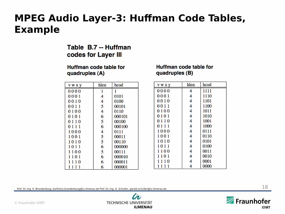
MPEG Audio Layer-3: Huffman Code Tables, Example
Prof. Dr.-Ing. K. Brandenburg, [email protected] Prof. Dr.-Ing. G. Schuller, [email protected] 18
© Fraunhofer IDMT
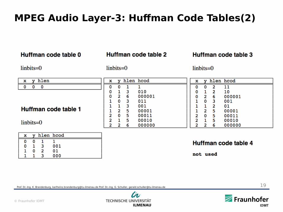
MPEG Audio Layer-3: Huffman Code Tables(2)
Prof. Dr.-Ing. K. Brandenburg, [email protected] Prof. Dr.-Ing. G. Schuller, [email protected] 19
© Fraunhofer IDMT
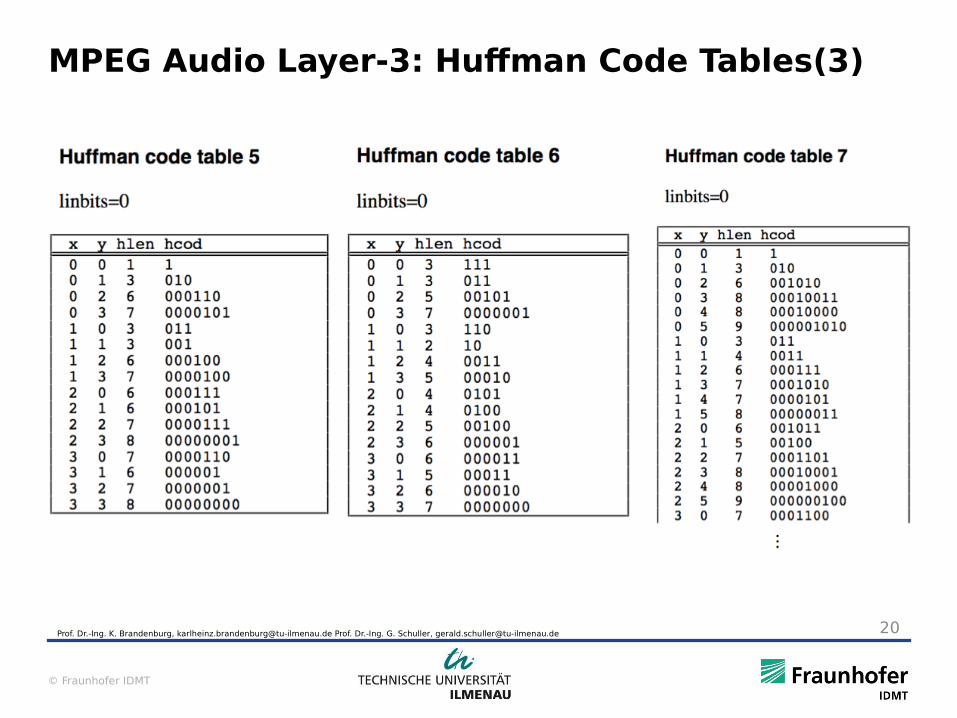
MPEG Audio Layer-3: Huffman Code Tables(3)
Prof. Dr.-Ing. K. Brandenburg, [email protected] Prof. Dr.-Ing. G. Schuller, [email protected] 20
© Fraunhofer IDMT
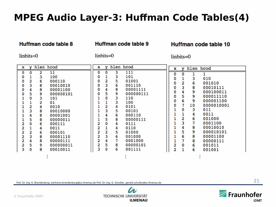
MPEG Audio Layer-3: Huffman Code Tables(4)
Prof. Dr.-Ing. K. Brandenburg, [email protected] Prof. Dr.-Ing. G. Schuller, [email protected] 21
© Fraunhofer IDMT
Joint Quantization / Coding Techniques (1)
Vector quantization Excellent coding efficiency at very low rates (<< 1 bit /
sample), but Perceptual control of distortion difficult control only total distortion for “group”
Application range: Used for intermediate quality / very low bit rate coding
e.g. MPEG-4 TwinVQ
Nice theoretical concept, today not in use in widely used standards!
The excitation codebook in CELP speech coding follows this paradigm.
Prof. Dr.-Ing. K. Brandenburg, [email protected] Prof. Dr.-Ing. G. Schuller, [email protected] 22
© Fraunhofer IDMT
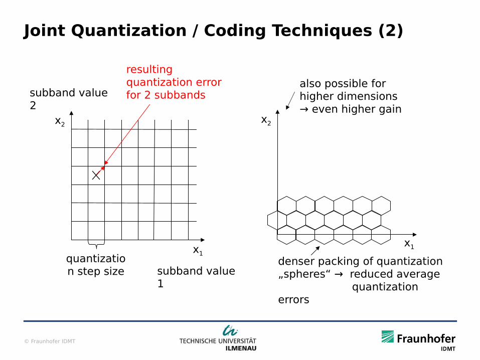
Joint Quantization / Coding Techniques (2)
quantization step size
resulting quantization error for 2 subbands
x1
x2
subband value 2
subband value 1
x1
also possible for higher dimensions→ even higher gain
denser packing of quantization„spheres“ → reduced average quantization errors
x2
© Fraunhofer IDMT
Encoding Strategies
Today‘s coding schemes provide large degree of flexibility Quantization noise profile over frequency Trade-off audio bandwidth vs. overall distortion Bit rate & coding mode Usage of optional tools (Temporal Noise Shaping, prediction)
Encoding strategy „intelligent“ part of encoding; determines quality Arena for specific know-how („secrets of audio coding“)
Prof. Dr.-Ing. K. Brandenburg, [email protected] Prof. Dr.-Ing. G. Schuller, [email protected] 24
© Fraunhofer IDMT
Constant Quality Coding
Goal: Coding with a pre-selected constant qualityProcedure: Estimate time & frequency dependent masking threshold Adjust quantizer step size to meet target distortion
Constant quality -> Variable bit rate
Applications: Storage media / transmission channels supporting variable rate e.g.
Storage on digital media; music on internet
Needs accurate perceptual model, often constant bit-rate coders sound better
Prof. Dr.-Ing. K. Brandenburg, [email protected] Prof. Dr.-Ing. G. Schuller, [email protected] 25
© Fraunhofer IDMT
Constant Rate Coding (1)
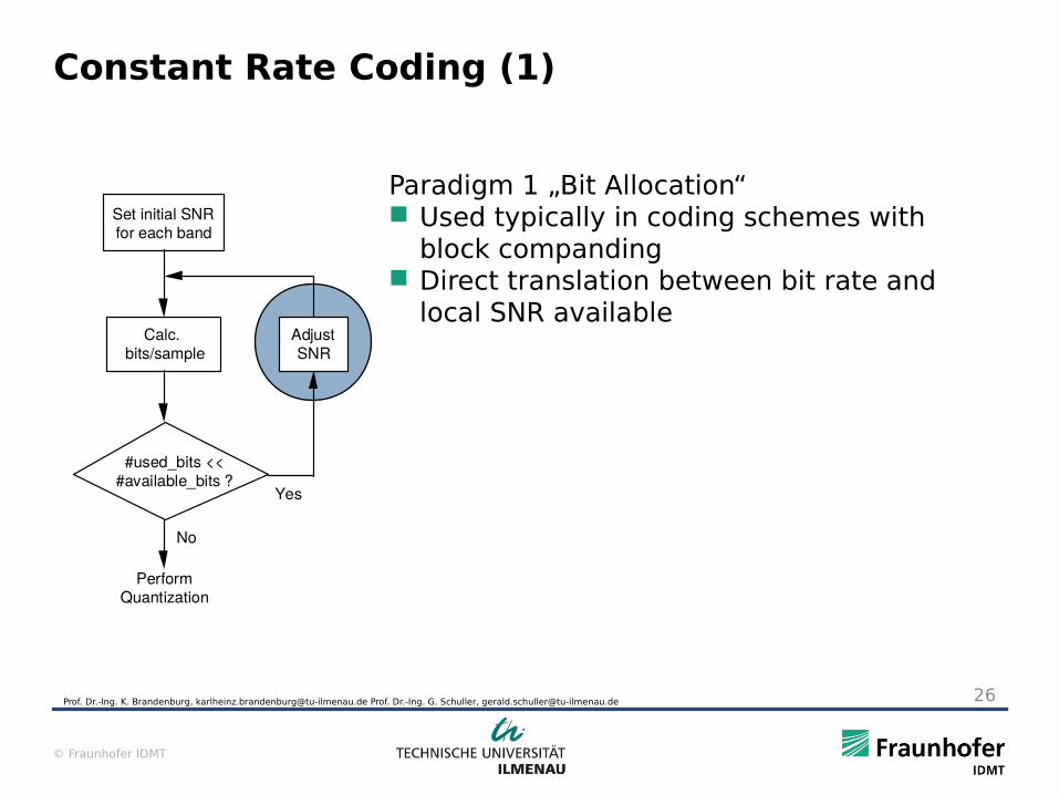
Paradigm 1 „Bit Allocation“ Used typically in coding schemes with
block companding Direct translation between bit rate and
local SNR available
Set initial SNRfor each band
Calc. bits/sample
#used_bits <<#available_bits ?
AdjustSNR
No
Yes
Perform Quantization
Prof. Dr.-Ing. K. Brandenburg, [email protected] Prof. Dr.-Ing. G. Schuller, [email protected] 26
© Fraunhofer IDMT
Constant Rate Coding (2)
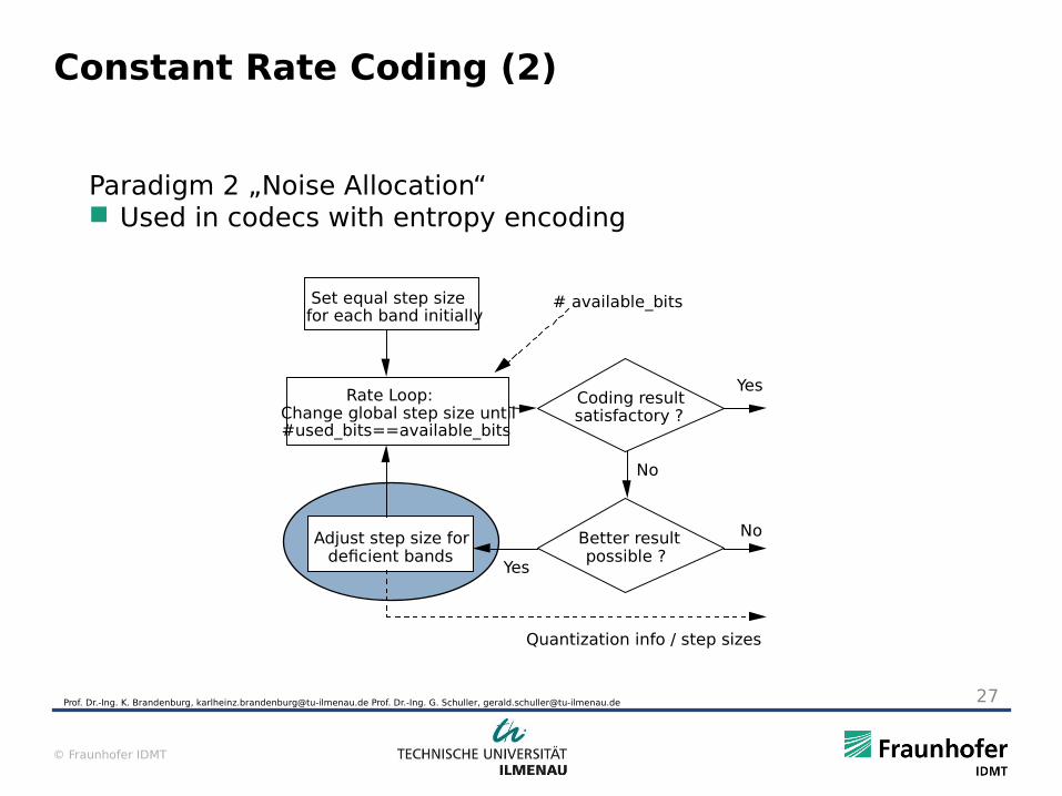
Paradigm 2 „Noise Allocation“ Used in codecs with entropy encoding
Set equal step sizefor each band initially
Rate Loop:Change global step size until#used_bits==available_bits
Adjust step size for deficient bands
Coding resultsatisfactory ?
Better result possible ?
Yes
No
No
Yes
Quantization info / step sizes
# available_bits
Prof. Dr.-Ing. K. Brandenburg, [email protected] Prof. Dr.-Ing. G. Schuller, [email protected] 27
© Fraunhofer IDMT
Constrained Variable Bit Rate Coding (Bit Reservoir)
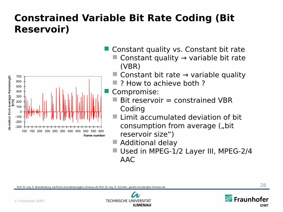
Constant quality vs. Constant bit rate Constant quality → variable bit rate
(VBR) Constant bit rate → variable quality ? How to achieve both ?
Compromise: Bit reservoir = constrained VBR
Coding Limit accumulated deviation of bit
consumption from average („bit reservoir size“)
Additional delay Used in MPEG-1/2 Layer III, MPEG-2/4
AAC
-300
-200
-100
0
100
200
300
400
500
600
700
100 150 200 250 300 350 400 450 500 550 600frame number
Prof. Dr.-Ing. K. Brandenburg, [email protected] Prof. Dr.-Ing. G. Schuller, [email protected] 28
© Fraunhofer IDMT
Constant vs. Variable Bit Rate Example
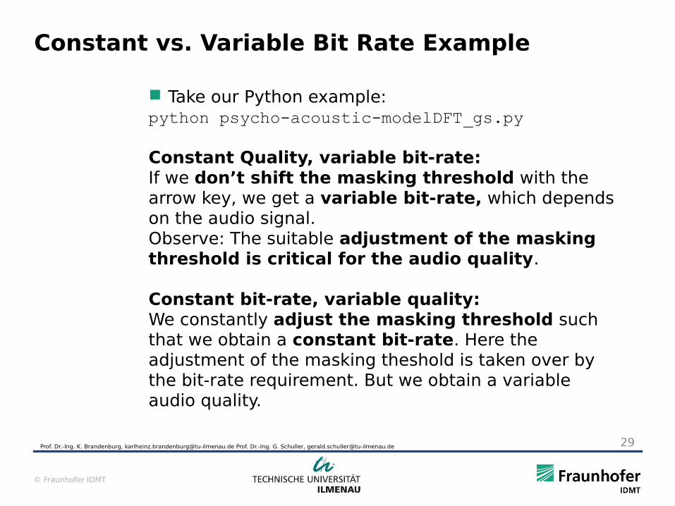
Take our Python example: python psycho-acoustic-modelDFT_gs.py
Constant Quality, variable bit-rate: If we don’t shift the masking threshold with the arrow key, we get a variable bit-rate, which depends on the audio signal.Observe: The suitable adjustment of the masking threshold is critical for the audio quality.
Constant bit-rate, variable quality:We constantly adjust the masking threshold such that we obtain a constant bit-rate. Here the adjustment of the masking theshold is taken over by the bit-rate requirement. But we obtain a variable audio quality.
Prof. Dr.-Ing. K. Brandenburg, [email protected] Prof. Dr.-Ing. G. Schuller, [email protected] 29
© Fraunhofer IDMT
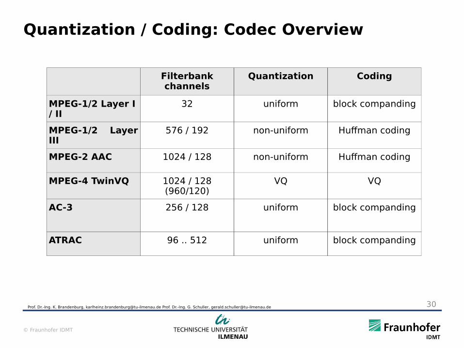
Quantization / Coding: Codec Overview
Prof. Dr.-Ing. K. Brandenburg, [email protected] Prof. Dr.-Ing. G. Schuller, [email protected] 30
Filterbank channels
Quantization Coding
MPEG-1/2 Layer I / II
32 uniform block companding
MPEG-1/2 Layer III
576 / 192 non-uniform Huffman coding
MPEG-2 AAC 1024 / 128 non-uniform Huffman coding
MPEG-4 TwinVQ 1024 / 128 (960/120)
VQ VQ
AC-3 256 / 128 uniform block companding
ATRAC 96 .. 512 uniform block companding
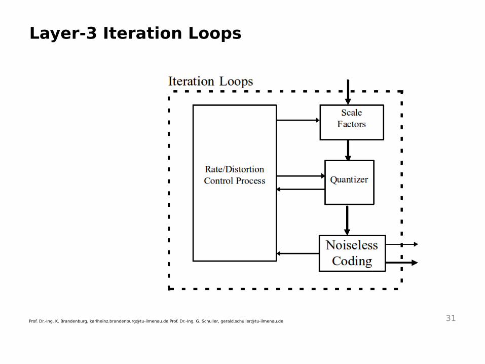
Layer-3 Iteration Loops
Prof. Dr.-Ing. K. Brandenburg, [email protected] Prof. Dr.-Ing. G. Schuller, [email protected] 31
Layer-3 : Outer Loop
Distortion Loop (control of the distortion) Saves the unquantized spectral values Compares the reconstructed values with the original Builds the actual distortion in the frequency domain Scaling by frequency groups with the amount of distortion Convergence of the iteration is not guaranteed
Prof. Dr.-Ing. K. Brandenburg, [email protected] Prof. Dr.-Ing. G. Schuller, [email protected] 32
© Fraunhofer IDMT
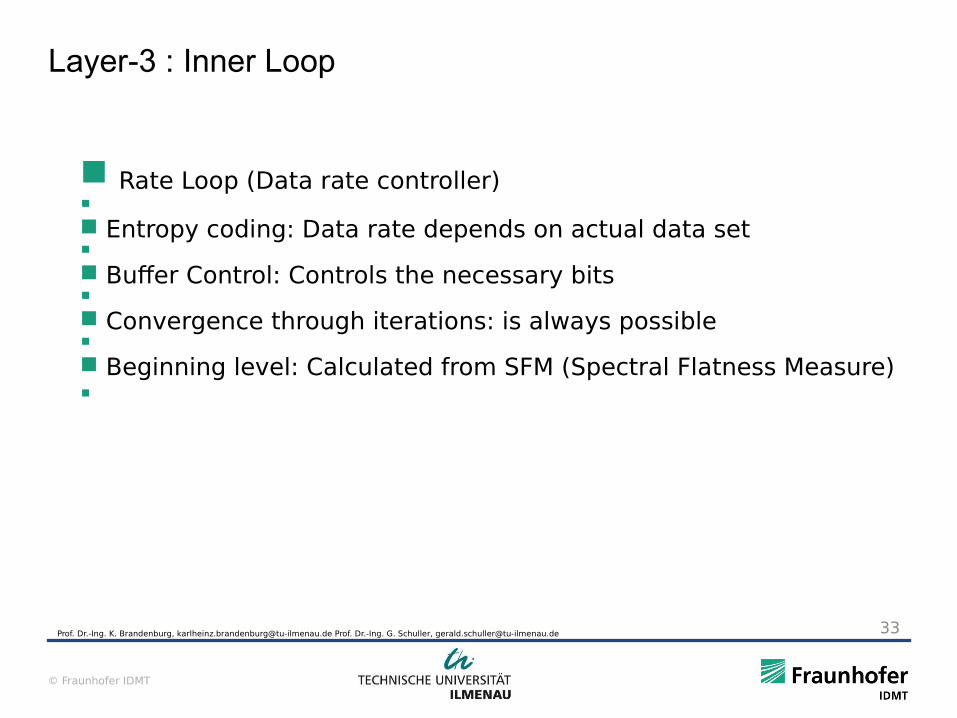
Layer-3 : Inner Loop
Rate Loop (Data rate controller) Entropy coding: Data rate depends on actual data set Buffer Control: Controls the necessary bits Convergence through iterations: is always possible Beginning level: Calculated from SFM (Spectral Flatness Measure)
Prof. Dr.-Ing. K. Brandenburg, [email protected] Prof. Dr.-Ing. G. Schuller, [email protected] 33


![ATSC Video and Audio Coding[1]](https://img.pdfslide.net/doc/110x75/577ce7441a28abf10394b704/atsc-video-and-audio-coding1.jpg)