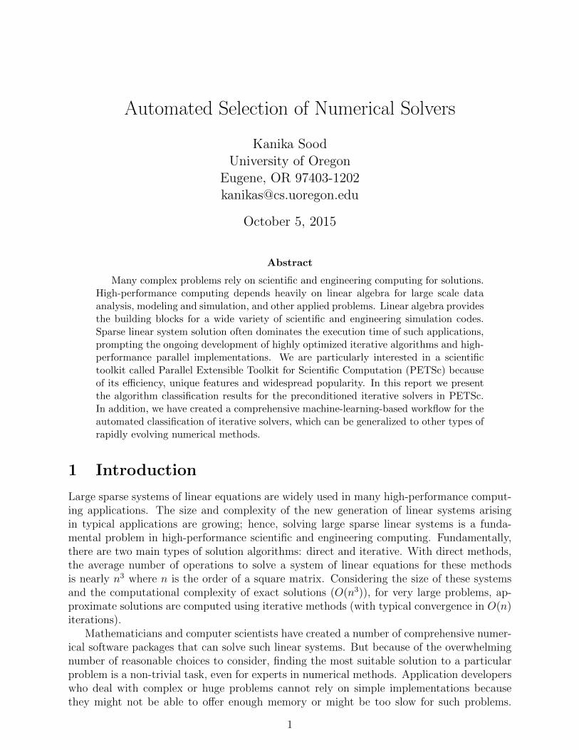
Automated Selection of Numerical Solvers

Kanika SoodUniversity of Oregon

Eugene, OR 97403-1202kanikas@cs.uoregon.edu

October 5, 2015

Abstract

Many complex problems rely on scientific and engineering computing for solutions.High-performance computing depends heavily on linear algebra for large scale dataanalysis, modeling and simulation, and other applied problems. Linear algebra providesthe building blocks for a wide variety of scientific and engineering simulation codes.Sparse linear system solution often dominates the execution time of such applications,prompting the ongoing development of highly optimized iterative algorithms and high-performance parallel implementations. We are particularly interested in a scientifictoolkit called Parallel Extensible Toolkit for Scientific Computation (PETSc) becauseof its efficiency, unique features and widespread popularity. In this report we presentthe algorithm classification results for the preconditioned iterative solvers in PETSc.In addition, we have created a comprehensive machine-learning-based workflow for theautomated classification of iterative solvers, which can be generalized to other types ofrapidly evolving numerical methods.

1 Introduction

Large sparse systems of linear equations are widely used in many high-performance comput-ing applications. The size and complexity of the new generation of linear systems arisingin typical applications are growing; hence, solving large sparse linear systems is a funda-mental problem in high-performance scientific and engineering computing. Fundamentally,there are two main types of solution algorithms: direct and iterative. With direct methods,the average number of operations to solve a system of linear equations for these methodsis nearly n3 where n is the order of a square matrix. Considering the size of these systemsand the computational complexity of exact solutions (O(n3)), for very large problems, ap-proximate solutions are computed using iterative methods (with typical convergence in O(n)iterations).

Mathematicians and computer scientists have created a number of comprehensive numer-ical software packages that can solve such linear systems. But because of the overwhelmingnumber of reasonable choices to consider, finding the most suitable solution to a particularproblem is a non-trivial task, even for experts in numerical methods. Application developerswho deal with complex or huge problems cannot rely on simple implementations becausethey might not be able to offer enough memory or might be too slow for such problems.

1

Therefore they must use high-performance computing (HPC) libraries developed by oth-ers. The current high-performance implementations of numerical linear algebra software arebased on decades of applied mathematics and computer science research. Therefore, select-ing a suitable library and using it effectively to solve a given problem can require significantbackground in numerical analysis, HPC, software engineering, and the researcher’s domainscience. This makes the application developers face the challenge of predicting which methodwill converge fastest, or converge at all, for a given linear system. Indeed, discovering thebest approach to solving a linear algebra problem typically involves reading documentation(when available) or researching publications outside of the developer’s area of expertise aswell as experimenting, across software options. While continuous advances in numericalanalysis and HPC libraries allow scientists and engineers to solve larger and more complexproblems than ever before, the likelihood that a user will identify the most relevant andwell-performing solution method is steadily decreasing. We apply several machine-learningtechniques to help make this decision based on relatively few, easily computable propertiesof the input linear system.

This work can provide support for identifying good solution methods for sparse linearsystems to existing taxonomies that aid developers in translating linear algebra algorithmsto numerical software, which do not have such support for sparse matrices at present. Onesuch taxonomy is Lighthouse [3], which is an open-source Web application that currentlyserves as a guide to the dense linear system solver methods.We plan to work on expandingthe Lighthouse framework for the production of matrix algebra software by adding supportfor sparse matrix algebra computations. The approach we follow for solver selection is to usemachine-learning algorithms to generate functions to map linear systems to suitable solvers.This contains two parts, feature extraction and classification. The feature extractor computesnumerical quantities, called features or properties, such as structural and spectral estimatesof the given linear system. The set of features is designed to represent the characteristics ofthe system that are predictive of the performance of solvers. The classifier maps the givenfeature values to a choice of solver. The task of the learning algorithm is to choose a subsetof the features, hereby referred to as feature selection, and associate the values of the selectedfeatures to the choice of the solver.

The contributions in this report can be summarized as follows.

• A generalizable machine learning-based workflow for classifying arbitrary sparse linearsystems using different-sized feature sets.

• Comparison of several machine-learning algorithms’ performance for classifying thePortable, Extensible Toolkit for Scientific Computation (PETSc) [2] solvers.

• Suggestions for good solver-preconditioner configurations for a given linear system.

• A set of solver-preconditioner configurations that are most likely to perform well.

2 Motivation

Several attempts have been made in the past to support automation of solver selection andconfiguration, but none of them are general enough or have produced a usable softwareinfrastructure that would enable users to apply them for their applications. Hence, our goalis to define an extensible methodology for classifying algorithms and software that supports

2

reusability and can also be used for the new solvers as they evolve. We apply variousmachine-learning algorithms to do the classification using Weka [21]. Weka is a tool thatcontains a collection of algorithms for data analysis and predictive modeling. We classifysolvers based on the properties of the linear system and select the solver configuration thathas been determined to perform best based on an extensive training set of problems.

In the past, many researchers have used machine-learning to identify “good” solversin the context of parallel nonlinear PDE solution [8, 10, 28]. Depending on the conditionsspecified in the simulation code, some matrices are weakly diagonally dominant (difficult tosolve), whereas others are strongly diagonally dominant (easy to solve). For matrices that areweakly diagonally dominant, this machine-learning framework was successful in identifyingsolvers with expensive preconditioners (such as BoomerAMG [34]). It was also successfulin identifying that very simple solvers (such as Jacobi [30]) would be fairly good for thestrongly diagonally dominant. The success of the limited-domain exploration motivated thework presented in this report, which covers a wider variety of domains and considers a muchgreater number of machine-learning methods.

3 Background

Existing numerical software taxonomy approaches are general and support relatively stand-alone algorithms. However, these approaches do not accommodate tasks for which no libraryimplementation exists, or tasks that involve more complex software packages. For instance,the functionality of large HPC toolkits, such as Trilinos [4] and PETSc, is difficult or ratherimpossible to represent and maintain in most previous taxonomies, which at present simplydirect the user to the toolkit’s home pages and do not provide any support for selectingsolution methods based on performance requirements. In this report we focus on addingsupport in our larger project, Lighthouse, in the area of preconditioned iterative solvers withPETSc.

PETSc provides good support for getting started with the toolkit. There are many waysof downloading PETSc: using a Git repository, installing a Debian package, or following adirect web download link. Once PETSc has been successfully installed, it is easy to find theguidelines to configure and build with the help of appropriate PETSc tutorials and otheronline documentation. Mandatory packages are automatically downloaded, configured, builtand installed with PETSc. A number of PETSc examples are also available to instruct theuser on writing PETSc programs and setting various command line options.

Selecting the appropriate PETSc algorithms, however, presents substantial difficulties. Asparse linear solver is typically paired with a preconditioner. To the uninformed user, the setof parallel Krylov methods and preconditioners contained in PETSc, summarized in Table 1,can be overwhelming because there are more than 300 possible pairings. Moreover, eachsolver-preconditioner pair can be configured through a set of algorithm-specific parameters,further expanding the search space. From this collection, the best choices for iterative solversand preconditioners for a given linear system, depend on properties of its coefficient matrixand may also depend on the physics of the problem. Choosing a solution configurationrequires a search of the extensive numerical linear algebra literature and may also requireintense document reading or knowledge in the domain. The users may or may not havethe expertise, knowledge and time required to do these tasks, therefore making the selectionprocess very challenging.

3

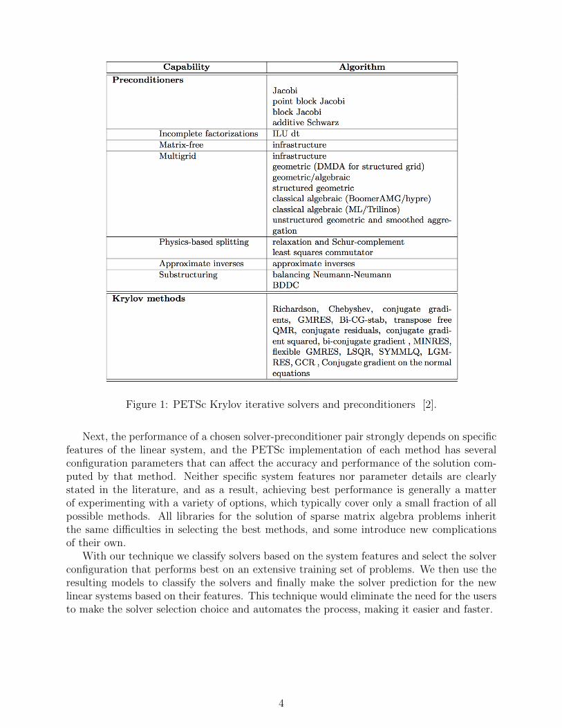
Figure 1: PETSc Krylov iterative solvers and preconditioners [2].

Next, the performance of a chosen solver-preconditioner pair strongly depends on specificfeatures of the linear system, and the PETSc implementation of each method has severalconfiguration parameters that can affect the accuracy and performance of the solution com-puted by that method. Neither specific system features nor parameter details are clearlystated in the literature, and as a result, achieving best performance is generally a matterof experimenting with a variety of options, which typically cover only a small fraction of allpossible methods. All libraries for the solution of sparse matrix algebra problems inheritthe same difficulties in selecting the best methods, and some introduce new complicationsof their own.

With our technique we classify solvers based on the system features and select the solverconfiguration that performs best on an extensive training set of problems. We then use theresulting models to classify the solvers and finally make the solver prediction for the newlinear systems based on their features. This technique would eliminate the need for the usersto make the solver selection choice and automates the process, making it easier and faster.

4

4 Approach

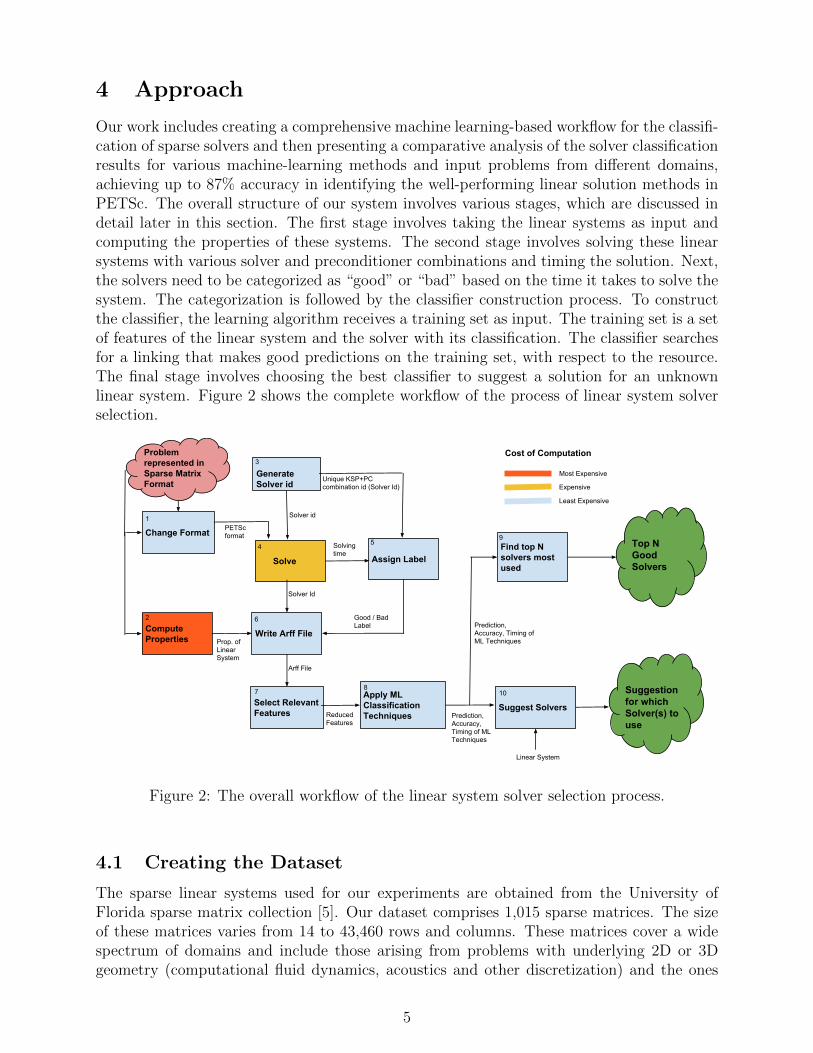
Our work includes creating a comprehensive machine learning-based workflow for the classifi-cation of sparse solvers and then presenting a comparative analysis of the solver classificationresults for various machine-learning methods and input problems from different domains,achieving up to 87% accuracy in identifying the well-performing linear solution methods inPETSc. The overall structure of our system involves various stages, which are discussed indetail later in this section. The first stage involves taking the linear systems as input andcomputing the properties of these systems. The second stage involves solving these linearsystems with various solver and preconditioner combinations and timing the solution. Next,the solvers need to be categorized as “good” or “bad” based on the time it takes to solve thesystem. The categorization is followed by the classifier construction process. To constructthe classifier, the learning algorithm receives a training set as input. The training set is a setof features of the linear system and the solver with its classification. The classifier searchesfor a linking that makes good predictions on the training set, with respect to the resource.The final stage involves choosing the best classifier to suggest a solution for an unknownlinear system. Figure 2 shows the complete workflow of the process of linear system solverselection.

Change Format

Compute Properties

Solve Assign Label

PETSc format

Write Arff File

Good / Bad Label

Solver Id

Select Relevant Features

Arff File

Find top N solvers most used

Top N Good Solvers

Suggest Solvers

Linear System

Suggestion for which Solver(s) to use

Problem represented in Sparse Matrix Format

Generate Solver id

Solver id

Unique KSP+PC combination id (Solver Id)

Apply ML Classification TechniquesReduced

Features

Prediction, Accuracy, Timing of ML TechniquesProp. of

LinearSystem

Solving time

Prediction, Accuracy, Timing of ML Techniques

1

2

3

4 5

6

7 8

9

10

Most Expensive

Least Expensive

Expensive

Cost of Computation

Figure 2: The overall workflow of the linear system solver selection process.

4.1 Creating the Dataset

The sparse linear systems used for our experiments are obtained from the University ofFlorida sparse matrix collection [5]. Our dataset comprises 1,015 sparse matrices. The sizeof these matrices varies from 14 to 43,460 rows and columns. These matrices cover a widespectrum of domains and include those arising from problems with underlying 2D or 3Dgeometry (computational fluid dynamics, acoustics and other discretization) and the ones

5

which typically do not have such geometry (optimization, circuit simulation and networksand graphs). Below are some of the kinds of the problems that are covered by our dataset:

• Electromagnetics problems

• Linear programming problems

• Acoustics problems

• Computational fluid dynamics problems

• Circuit simulation problems

• Undirected weighted graph problems

• Optimization problems

• Power network problems

• Undirected random graph problems

• Chemical process simulation problems

When using supervised machine-learning methods for building models, a common prob-lem is overfitting. Overfitting occurs when a model begins to “memorize” training datarather than “learning” to generalize from the trend. The chances of overfitting are reducedby the large variety of problem domains that our dataset covers.

The input matrices are in Matrix Market format [1]. For reading in parallel, MatrixMarket is not very suitable; hence, for all cases, serial and parallel, we pre-process andconvert the Matrix Market format to PETSc binary format.

4.2 Preparing Data for Training

Once we have the dataset ready, the next step is to convert the data in the training set into aform that is usable by Weka. The input to the learning process is Weka’s Attribute-RelationFile Format (ARFF) ASCII text file, which describes a list of instances that share someattributes. Each data point includes a list of feature values, the solver identifier, and a label.The solver identifier is unique to each pairing of specific Krylov method and preconditioner.So for M matrices, we have M ∗ N data points, N being the number of possible solvers.Because this number can be prohibitively large, we constructed the training set by computinga smaller number of randomly selected points. We labeled each data point as “good” or “bad”based on the performance of the solver on a matrix based on a threshold parameter b in therange 0,1 specifying how close the solver’s performance is to the known best performingmethod. For example, when b = 0.25, solvers whose performance for a given problem iswithin 25% of the best were labeled as “good”, while all other solvers were labeled as “bad”.The threshold used for labeling the dataset in this case was b = 0.35, which means thatmethods within the top 35% of the best solver time were labeled as good. This value of bwas chosen as the best among several sampled values between 0.01 and 0.45. We consideredbinary labels for classification, because our experiments with three-class labels showed that,with the given number of data points collected, they are not enough to be distributed inthree classes, as we need enough data points in each class. We do not consider ranking either,because binary classification has the greatest number of machine-learning methods availablefor classification.

6

4.3 Solving the linear systems

PETSc has a collection of parallel algorithms for direct solvers, Krylov iterative methods,and preconditioners that can be used in application codes written in C, C++, Fortranand Python. Our focus is on iterative Krylov methods and preconditioners. To solve thesparse linear systems derived from the input matrices, we used 154 preconditioner-solverconfigurations chosen from more than 300 valid options available in PETSc, with all right-hand side elements set to one. These 300 options can be expanded further as they areconfigurable with additional parameters, for both, solvers and preconditioners. We considerthe following preconditioners and solvers chosen from PETSc.

4.3.1 Preconditioners

Preconditioning refers to the process of applying a transformation on the original problemand brings it into a form that is more suitable for the solving methods. The main ideabehind applying a preconditioner is that, instead of solving Ax = b, solve M−1Ax = M−1busing a nonsingular m x m preconditioner M, which has the same solution x.

Here we mention the various preconditioners we considered and the subset of parametersfor them. The preconditioners are as follows:

1. Incomplete factorization preconditioners (ILU): ILU is an approximation of theLU (Lower Upper) factorization. LU factorization factors a matrix as the product ofthe lower and the upper triangular matrix.

Parameters: Factor levels which are the number of levels of fill for ILU.

Parameter values: 0, 1, 2 and 3.

2. Additive Schwarz method (ASM): Solves an equation approximately by splittingit into boundary value problems and adds the results.

Parameter considered: The amount of overlap between sub-domains.

Parameter values: 0, 1, 2 and 3.

3. Jacobi or diagonal: One of the simplest forms of preconditioning in which the pre-conditioner is the diagonal of the matrix as shown below.

M = diag(A) for M−1Ax = M−1 b.

4. Block Jacobi: It is similar to Jacobi, except that in this case, instead of the diagonal,the block-diagonal is chosen as the preconditioner (M).

5. Incomplete Cholesky factorization (ICC): It is a sparse approximation of theCholesky factorization. The Cholesky factorization A is A = LL∗ where L is a lowertriangular matrix. An incomplete Cholesky factorization is given by a sparse lowertriangular matrix K that is very close to L. The corresponding preconditioner isKK∗.

Parameter considered: Factor levels which are the number of levels of fill for ICC.

Parameter values: 0, 1, 2 and 3.

These and other Krylov methods are described in more detail in [31].

7

4.3.2 Solvers

Similar to preconditioners, solvers also have their own parameters. For this research we areconsidering only default parameters. We considered the following iterative solvers.

1. Generalized minimal residual method (GMRES): This method approximatesthe solution by the vector in a Krylov subspace with minimal residual. The Arnoldiiteration is used to find this vector.

2. The Flexible Generalized minimal residual method (FGMRES): It is a gen-eralization of GMRES that allows larger flexibility in the choice of solution subspacethan GMRES.

3. LGMRES: It augments the standard GMRES approximation space with approxima-tions to the error from previous restart cycles.

4. Conjugate gradient method (CG): This method starts with an initial guess of thesolution, with an initial residual and with an initial search direction.

5. Biconjugate Gradient Method (BICG): Implements the Biconjugate gradientmethod, similar to running the conjugate gradient on the normal equations.

6. Biconjugate gradient stabilized method (BCGStab): It is a stabilized versionof BiConjugate Gradient Squared method.

7. Improved Stabilized version of BiConjugate Gradient Squared (IBCGS): Itis an improved stabilized version of BiConjugate Gradient Squared method.

8. Transpose-Free Quasi-Minimal Residual Method (TFQMR): It is a quasi-minimal residual version of CGS. It retains the desirable convergence features of CGSand corrects its erratic behavior.

9. TCQMR: It is a variant of quasi-minimal residual provided by Tony Chan.

10. LSQR: This is an algorithm for sparse linear equations and sparse least squares.

11. Chebyshev: This method requires enough knowledge about the spectrum of the ma-trix, which is an upper estimate for the upper eigenvalue and lower estimate for thelower eigenvalue. Chebyshev iteration method avoids the computation of inner prod-ucts as is necessary for the other methods.

We capture the time taken to solve the system, the number of iterations, and solver andpreconditioning options, such as number of blocks and overlap.

4.4 Feature Computation

We used Anamod [20], which is a library of modules that uses PETSc functions, to computevarious properties of a system and extracted sixty-eight features shown in Figure 1 of thecoefficient matrices. These features include several categories as mentioned below:

1. Simple (norm-like quantities): Properties which are estimates of the departurefrom normality such as 1-norm, infinity-norm and Frobenius-norms of the matrix, aswell as these norms taken of the symmetric and non-symmetric part of the matrix.

8

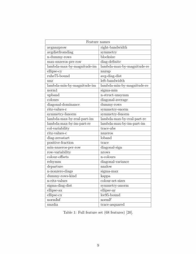
Feature names

avgnnzprow right-bandwidthavgdistfromdiag symmetryn-dummy-rows blocksizemax-nnzeros-per-row diag-definitelambda-max-by-magnitude-im lambda-max-by-magnitude-reellipse-cy nnzupruhe75-bound avg-diag-distnnz left-bandwidthlambda-min-by-magnitude-im lambda-min-by-magnitude-renorm1 sigma-minupband n-struct-unsymmcolours diagonal-averagediagonal-dominance dummy-rowsritz-values-r symmetry-snormsymmetry-fanorm symmetry-fsnormlambda-max-by-real-part-im lambda-max-by-real-part-relambda-max-by-im-part-re lambda-max-by-im-part-imcol-variability trace-absritz-values-c nnzerosdiag-zerostart lobandpositive-fraction tracemin-nnzeros-per-row diagonal-signrow-variability nrowscolour-offsets n-coloursrelsymm diagonal-variancedeparture nnzlown-nonzero-diags sigma-maxdummy-rows-kind kappan-ritz-values colour-set-sizessigma-diag-dist symmetry-anormellipse-ax ellipse-ayellipse-cx lee95-boundnormInf normFnnzdia trace-asquared

Table 1: Full feature set (68 features) [20].

9

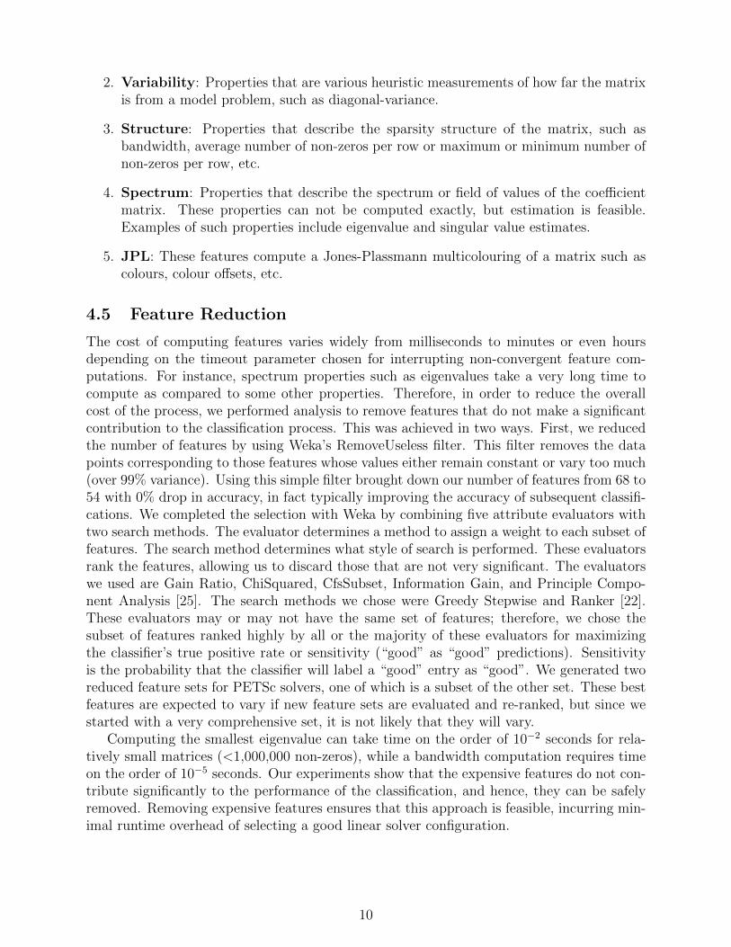
2. Variability: Properties that are various heuristic measurements of how far the matrixis from a model problem, such as diagonal-variance.

3. Structure: Properties that describe the sparsity structure of the matrix, such asbandwidth, average number of non-zeros per row or maximum or minimum number ofnon-zeros per row, etc.

4. Spectrum: Properties that describe the spectrum or field of values of the coefficientmatrix. These properties can not be computed exactly, but estimation is feasible.Examples of such properties include eigenvalue and singular value estimates.

5. JPL: These features compute a Jones-Plassmann multicolouring of a matrix such ascolours, colour offsets, etc.

4.5 Feature Reduction

The cost of computing features varies widely from milliseconds to minutes or even hoursdepending on the timeout parameter chosen for interrupting non-convergent feature com-putations. For instance, spectrum properties such as eigenvalues take a very long time tocompute as compared to some other properties. Therefore, in order to reduce the overallcost of the process, we performed analysis to remove features that do not make a significantcontribution to the classification process. This was achieved in two ways. First, we reducedthe number of features by using Weka’s RemoveUseless filter. This filter removes the datapoints corresponding to those features whose values either remain constant or vary too much(over 99% variance). Using this simple filter brought down our number of features from 68 to54 with 0% drop in accuracy, in fact typically improving the accuracy of subsequent classifi-cations. We completed the selection with Weka by combining five attribute evaluators withtwo search methods. The evaluator determines a method to assign a weight to each subset offeatures. The search method determines what style of search is performed. These evaluatorsrank the features, allowing us to discard those that are not very significant. The evaluatorswe used are Gain Ratio, ChiSquared, CfsSubset, Information Gain, and Principle Compo-nent Analysis [25]. The search methods we chose were Greedy Stepwise and Ranker [22].These evaluators may or may not have the same set of features; therefore, we chose thesubset of features ranked highly by all or the majority of these evaluators for maximizingthe classifier’s true positive rate or sensitivity (“good” as “good” predictions). Sensitivityis the probability that the classifier will label a “good” entry as “good”. We generated tworeduced feature sets for PETSc solvers, one of which is a subset of the other set. These bestfeatures are expected to vary if new feature sets are evaluated and re-ranked, but since westarted with a very comprehensive set, it is not likely that they will vary.

Computing the smallest eigenvalue can take time on the order of 10−2 seconds for rela-tively small matrices (<1,000,000 non-zeros), while a bandwidth computation requires timeon the order of 10−5 seconds. Our experiments show that the expensive features do not con-tribute significantly to the performance of the classification, and hence, they can be safelyremoved. Removing expensive features ensures that this approach is feasible, incurring min-imal runtime overhead of selecting a good linear solver configuration.

10

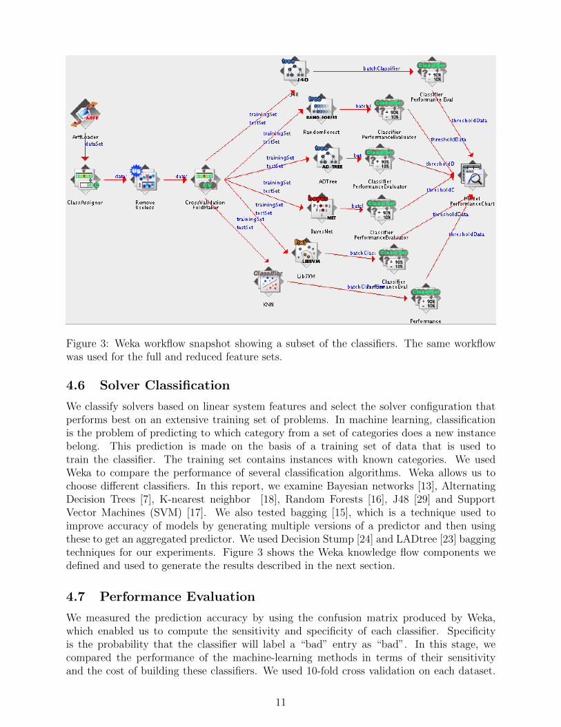
Figure 3: Weka workflow snapshot showing a subset of the classifiers. The same workflowwas used for the full and reduced feature sets.

4.6 Solver Classification

We classify solvers based on linear system features and select the solver configuration thatperforms best on an extensive training set of problems. In machine learning, classificationis the problem of predicting to which category from a set of categories does a new instancebelong. This prediction is made on the basis of a training set of data that is used totrain the classifier. The training set contains instances with known categories. We usedWeka to compare the performance of several classification algorithms. Weka allows us tochoose different classifiers. In this report, we examine Bayesian networks [13], AlternatingDecision Trees [7], K-nearest neighbor [18], Random Forests [16], J48 [29] and SupportVector Machines (SVM) [17]. We also tested bagging [15], which is a technique used toimprove accuracy of models by generating multiple versions of a predictor and then usingthese to get an aggregated predictor. We used Decision Stump [24] and LADtree [23] baggingtechniques for our experiments. Figure 3 shows the Weka knowledge flow components wedefined and used to generate the results described in the next section.

4.7 Performance Evaluation

We measured the prediction accuracy by using the confusion matrix produced by Weka,which enabled us to compute the sensitivity and specificity of each classifier. Specificityis the probability that the classifier will label a “bad” entry as “bad”. In this stage, wecompared the performance of the machine-learning methods in terms of their sensitivityand the cost of building these classifiers. We used 10-fold cross validation on each dataset.

11

Feature name ReducedFeature Set 1

(RS1)

ReducedFeature Set 2

(RS2)avg-diagonal-dist X Xnnz Xnorm1 X Xmin-nnzeros-per-row X Xnorm1 X Xrow-variability X Xn-nonzero-diags Xkappa X X

Table 2: Reduced feature sets RS1 and RS2.

0%#10%#20%#30%#40%#50%#60%#70%#80%#90%#

100%#LibSVM'

RF'

BayesNet*'

knn'

ADT'

J48'

All#Features# Reduced#Set#1# Reduced#Set#2#

Method TAll TRS1 TRS2

LibSVM 6.88 1.94 1.79RF 2.67 2.40 1.43BayesNet 0.10 0.02 0.01knn 0.001 0.001 0.001ADTree 0.74 0.18 0.09J48 0.24 0.19 0.06

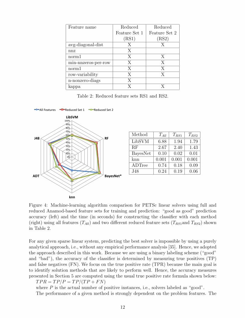
Figure 4: Machine-learning algorithm comparison for PETSc linear solvers using full andreduced Anamod-based feature sets for training and prediction: “good as good” predictionaccuracy (left) and the time (in seconds) for constructing the classifier with each method(right) using all features (TAll) and two different reduced feature sets (TRS1and TRS2) shownin Table 2.

For any given sparse linear system, predicting the best solver is impossible by using a purelyanalytical approach, i.e., without any empirical performance analysis [35]. Hence, we adoptedthe approach described in this work. Because we are using a binary labeling scheme (“good”and “bad”), the accuracy of the classifier is determined by measuring true positives (TP)and false negatives (FN). We focus on the true positive rate (TPR) because the main goal isto identify solution methods that are likely to perform well. Hence, the accuracy measurespresented in Section 5 are computed using the usual true positive rate formula shown below:

TPR = TP/P = TP/(TP + FN)where P is the actual number of positive instances, i.e., solvers labeled as “good”.The performance of a given method is strongly dependent on the problem features. The

12

Occurrence KrylovMethod

Preconditioner

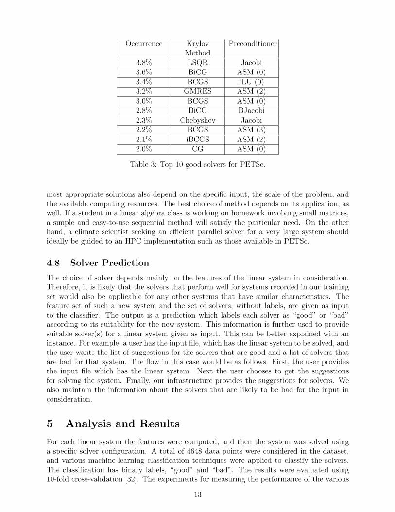
3.8% LSQR Jacobi3.6% BiCG ASM (0)3.4% BCGS ILU (0)3.2% GMRES ASM (2)3.0% BCGS ASM (0)2.8% BiCG BJacobi2.3% Chebyshev Jacobi2.2% BCGS ASM (3)2.1% iBCGS ASM (2)2.0% CG ASM (0)

Table 3: Top 10 good solvers for PETSc.

most appropriate solutions also depend on the specific input, the scale of the problem, andthe available computing resources. The best choice of method depends on its application, aswell. If a student in a linear algebra class is working on homework involving small matrices,a simple and easy-to-use sequential method will satisfy the particular need. On the otherhand, a climate scientist seeking an efficient parallel solver for a very large system shouldideally be guided to an HPC implementation such as those available in PETSc.

4.8 Solver Prediction

The choice of solver depends mainly on the features of the linear system in consideration.Therefore, it is likely that the solvers that perform well for systems recorded in our trainingset would also be applicable for any other systems that have similar characteristics. Thefeature set of such a new system and the set of solvers, without labels, are given as inputto the classifier. The output is a prediction which labels each solver as “good” or “bad”according to its suitability for the new system. This information is further used to providesuitable solver(s) for a linear system given as input. This can be better explained with aninstance. For example, a user has the input file, which has the linear system to be solved, andthe user wants the list of suggestions for the solvers that are good and a list of solvers thatare bad for that system. The flow in this case would be as follows. First, the user providesthe input file which has the linear system. Next the user chooses to get the suggestionsfor solving the system. Finally, our infrastructure provides the suggestions for solvers. Wealso maintain the information about the solvers that are likely to be bad for the input inconsideration.

5 Analysis and Results

For each linear system the features were computed, and then the system was solved usinga specific solver configuration. A total of 4648 data points were considered in the dataset,and various machine-learning classification techniques were applied to classify the solvers.The classification has binary labels, “good” and “bad”. The results were evaluated using10-fold cross-validation [32]. The experiments for measuring the performance of the various

13

solver and preconditioner combinations in PETSc version 3.5.3 were performed on the BlueGene/Q supercomputer. The classification was performed on an Intel Core i5 MacBook Pro.

In our work, we focus mainly on true positives (i.e., best-performing solvers predictedas best-performing). Our experiments include performance for the full feature set and tworeduced feature sets. The first reduced set (RS1) is obtained by removing the features thatdo not contribute much towards the classification using Weka. The features in RS1 are:

1. avg-diag-dist: This is the average diagonal distance.

2. nnz: The total number of non-zeros in the matrix.

3. norm1: The maximum absolute column sum of A. It is given by the following formula.

One norm of A is max1≤j≤m

(∑m

i=1 |ai,j|)

4. col-variability: The element variability in columns.

5. min-nnzeros-per-row: The minimum number of non-zeros per rows.

6. row-variability: The element variability in rows.

7. n-nonzero-diags: The number of diagonals that have any nonzero element.

8. kappa: The estimated condition number of the matrix.

We further reduced RS1 to create Reduced Set 2 (RS2). This was achieved by removingsize-dependent features to evaluate the sensitivity of the classification process to the problemsize. Our observations reveal that removing size-based features has minimal impact on theaccuracy of the best classification. This interesting finding suggests that future classifierscan be created, without including data points for a wide range of matrix sizes. Among allmachine-learning methods we applied, BayesNet showed the best performance in all cases:full feature set as well as both the reduced feature sets (RS1 and RS2). The accuracy was87.60% with the full feature set, which has 68 input features. Using only eight compu-tationally inexpensive features in RS1, the BayesNet-based classifier predicted good solverscorrectly 86.91% of the time and 86.40% with RS2. RS1 and RS2 are shown in Figure 2. Fig-ure 4 shows the true positive prediction accuracy of several of the machine-learning methodswe tested for the full and reduced feature sets. We tested more methods than are includedin the figure, but none of them performed better than the best method shown in the figure.We tested a subset of the configurations possible for the solvers and preconditioners andobserved the occurrence of each of them to conclude which methods and preconditionerswere the most successful. Table 5 summarizes these configurations that were most likely toperform well among all the configurations we tested.

6 Related Work

There have been several attempts and software developments for selecting efficient solversfor linear systems. One such attempt is the Linear System Analyzer (LSA) [14] which isa component-based environment that allows the user to specify combinations of precondi-tioner and solver, without the need to know the details of the implementation. Other similar

14

approaches include: a poly-iterative linear solver [6], which applies several iterative meth-ods simultaneously to the same system; a composite multi-method solver [11, 12], where asequence of solvers is applied to the linear system; an adaptive multi-method solvers ap-proach [9, 26], where linear solvers are selected dynamically to match closely the evolvingnumeric properties of the linear systems; and a self-adapting large scale solver architecture(SALSA) [19], which uses statistical techniques such as principal component analysis forsolver selection.

7 Challenges

There were many challenges involved in the entire process of providing solver suggestionsfor sparse linear systems. In this section we summarize those challenges. Given a linearsystem, we derived the features of those systems. The time required to compute the featuresvaried depending on the category of the features. For instance, the cost of computation ofthe spectral features, is theoretically much higher than even solving the system. Runningthe solvers is yet another expensive step, and some of the methods do not even converge.Another challenging issue arose during the format conversion from Matrix Market to PETScbinary format. Matrix Market format does not store all diagonal entries, but PETSc formatrequires all diagonal entries to be stored, even when they are zero. This resulted in errorsfor many of the matrices.

8 Conclusion

This work demonstrates how machine-learning can be applied to select solution algorithmsfor large sparse linear systems. Given that solutions of linear systems are involved in manyscientific and engineering problems, there is immense scope in automating the process ofsolver selection. Our study shows that we can rank the properties of matrices according totheir share of contribution towards the classification process. The correlation between matrixproperties and linear solvers is a recent topic of study among researchers, and understandingthe structure of the classifiers can result in strong contributions in this field.

There can be many solutions for a linear system, and there also can be many machine-learning algorithms that can be applied to choose among these solutions. The more optionsavailable to choose from, the more confounding it becomes. We present [27, 33] a compara-tive analysis of the solver classification results for a variety of input problems belonging todifferent domains and various machine-learning methods, achieving up to 87% accuracy inidentifying the well-performing linear solution methods in PETSc.

Acknowledgment

This work is supported by the U.S. Department of Energy Office of Science (Contract No.DE-SC0013869) and by the National Science Foundation (NSF) awards CCF-1219089, CCF-155063 and CCF-1550202.

15

References

[1] Matrix Market. http://math.nist.gov/MatrixMarket/, 2015.

[2] Portable, Extensible Toolkit for Scientific Computation (PETSc).http://www.mcs.anl.gov/petsc/, 2015.

[3] The Lighthouse Project. http://lighthousehpc.github.io/lighthouse/, 2015.

[4] The Trilinos Project. http://trilinos.sandia.gov/, 2015.

[5] The University of Florida Sparse Matrix Collection.http://www.cise.ufl.edu/research/sparse/matrices/, 2015.

[6] R. Barrett, M. Berry, J. Dongarra, V. Eijkhout, and C. Romine. Algorithmic bombard-ment for the iterative solution of linear systems: a poly-iterative approach. Journal ofComputational and applied Mathematics, 74(1):91–109, 1996.

[7] S. Bhowmick, V. Eijkhout, Y. Freund, E. Fuentes, and D. Keyes. Application of alter-nating decision trees in selecting sparse linear solvers. 2010.

[8] S. Bhowmick, D. Kaushik, L. McInnes, B. Norris, and P. Raghavan. Parallel adaptivesolvers in compressible PETSc-FUN3D simulations. In Proceedings of the 17th Interna-tional Conference on Parallel CFD, 2005.

[9] S. Bhowmick, L. McInnes, B. Norris, and P. Raghavan. The role of multi-method linearsolvers in PDE-based simulations. In Computational Science and Its ApplicationsICCSA2003, pages 828–839. Springer, 2003.

[10] S. Bhowmick, P. Raghavan, L. McInnes, and B. Norris. Faster PDE-based simulationsusing robust composite linear solvers. Future Generation Computer Systems, 20(3):373–387, 2004.

[11] S. Bhowmick, P. Raghavan, L. McInnes, and B. Norris. Faster PDE-based simulationsusing robust composite linear solvers. Future Generation Computer Systems, 20(3):373–387, 2004.

[12] S. Bhowmick, P. Raghavan, and K. Teranishi. A combinatorial scheme for develop-ing efficient composite solvers. In Computational ScienceICCS 2002, pages 325–334.Springer, 2002.

[13] C. Bielza and P. Larranaga. Discrete Bayesian Network classifiers: A survey. ACMComput. Surv., 47(1):5:1–5:43, July 2014.

[14] R. Bramley, D. Gannon, T. Stuckey, J. Villacis, E. Akman, J. Balasubramanian, F. Breg,S. Diwan, and M. Govindaraju. The linear system analyzer. Technical report, TechnicalReport TR511, Indiana University, 1998.

[15] L. Breiman. Bagging predictors. Machine Learning, 24(2):123–140, 1996.

[16] L. Breiman. Random forests. Machine Learning, 45(1):5–32, Oct. 2001.

16

[17] C. Cortes and V. Vapnik. Support-vector networks. Machine Learning, 20(3):273–297,1995.

[18] P. Cunningham and S. J. Delany. k-nearest neighbour classifiers. Multiple ClassifierSystems, pages 1–17, 2007.

[19] J. Demmel, J. Dongarra, V. Eijkhout, E. Fuentes, A. Petitet, R. Vuduc, R. C. Whaley,and K. Yelick. Self-adapting linear algebra algorithms and software. Proceedings of theIEEE, 93(2):293–312, 2005.

[20] V. Eijkhout and E. Fuentes. A proposed standard for matrix metadata. TechnicalReport ICL-UT 03-02, University of Tennessee, 2003.

[21] M. Hall, E. Frank, G. Holmes, B. Pfahringer, P. Reutemann, and I. H. Witten. TheWEKA data mining software: An update. SIGKDD Explorations, 11, 2009.

[22] N. Z. Hamilton. Correlation-based feature subset selection for machine learning. 1998.

[23] G. Holmes, B. Pfahringer, R. Kirkby, E. Frank, and M. Hall. Multiclass alternatingdecision trees. In ECML, pages 161–172. Springer, 2001.

[24] W. Iba and P. Langley. Induction of one-level decision trees. In Proceedings of the ninthinternational conference on machine learning, pages 233–240, 1992.

[25] R. Kirkby, E. Frank, and P. Reutemann. Weka explorer user guide for version 3-5-6.2007.

[26] L. McInnes, B. Norris, S. Bhowmick, and P. Raghavan. Adaptive sparse linear solversfor implicit cfd using newton-krylov algorithms. In Proceedings of the Second MITConference on Computational Fluid and Solid Mechanics, volume 2, pages 1024–1028,2003.

[27] P. Motter, K. Sood, E. Jessup, and B. Norris. Lighthouse : An automated solver selec-tion tool. In Software Engineering for High Performance Computing in ComputationalScience and Engineering, Austin, Texas, 2015.

[28] B. Norris, L. C. McInnes, S. Bhowmick, and L. Li. Adaptive numerical components forpde-based simulations. PAMM, 7(1):1140509–1140510, 2007.

[29] R. Quinlan. C4.5: Programs for Machine Learning. Morgan Kaufmann Publishers, SanMateo, CA, 1993.

[30] H. Rutishauser. The Jacobi method for real symmetric matrices. Numerische Mathe-matik, 9(1):1–10, 1966.

[31] Y. Saad. Iterative methods for sparse linear systems. Siam, 2003.

[32] J. Shao. Linear model selection by cross-validation. Journal of the American StatisticalAssociation, 88(422):486–494, 1993.

[33] K. Sood, B. Norris, and E. Jessup. Lighthouse: A taxonomy-based solver selection tool.In Software Engineering for Parallel Systems, Pittsburgh, Pennsylvania, 2015.

17

[34] U. M. Yang et al. BoomerAMG: a parallel algebraic multigrid solver and preconditioner.Applied Numerical Mathematics, 41(1):155–177, 2002.

[35] W. Zhao, R. Chellappa, and N. Nandhakumar. Empirical performance analysis of lineardiscriminant classifiers. In Computer Vision and Pattern Recognition, 1998. Proceedings.1998 IEEE Computer Society Conference, pages 164–169. IEEE, 1998.

18