Embed Size (px)
Citation preview

ISSN 1670-8539
M.Sc. PROJECT REPORT
Þór Sigurðsson
Master of Science
Computer Science
May 2011
School of Computer Science
Reykjavík University
AUTOMATIC PLANNING IN WIND-ENERGYPRODUCTION USING ENSEMBLEFORECASTS


Project Report Committee:
Ari Kristinn Jónsson, SupervisorRector, Reykjavik University
Ólafur RögnvaldssonCEO, Institute for Meteorological Research
Yngvi BjörnssonAssociate Professor, Reykjavik University
Project report submitted to the School of Computer Scienceat Reykjavík University in partial fulfillment of
the requirements for the degree ofMaster of Sciencein Computer Science
May 2011
Automatic planning in wind-energy production usingensemble forecasts
by
Þór Sigurðsson

CopyrightÞór Sigurðsson
May 2011
Automatic planning in wind-energy production using ensembleforecasts
Þór Sigurðsson
May 2011
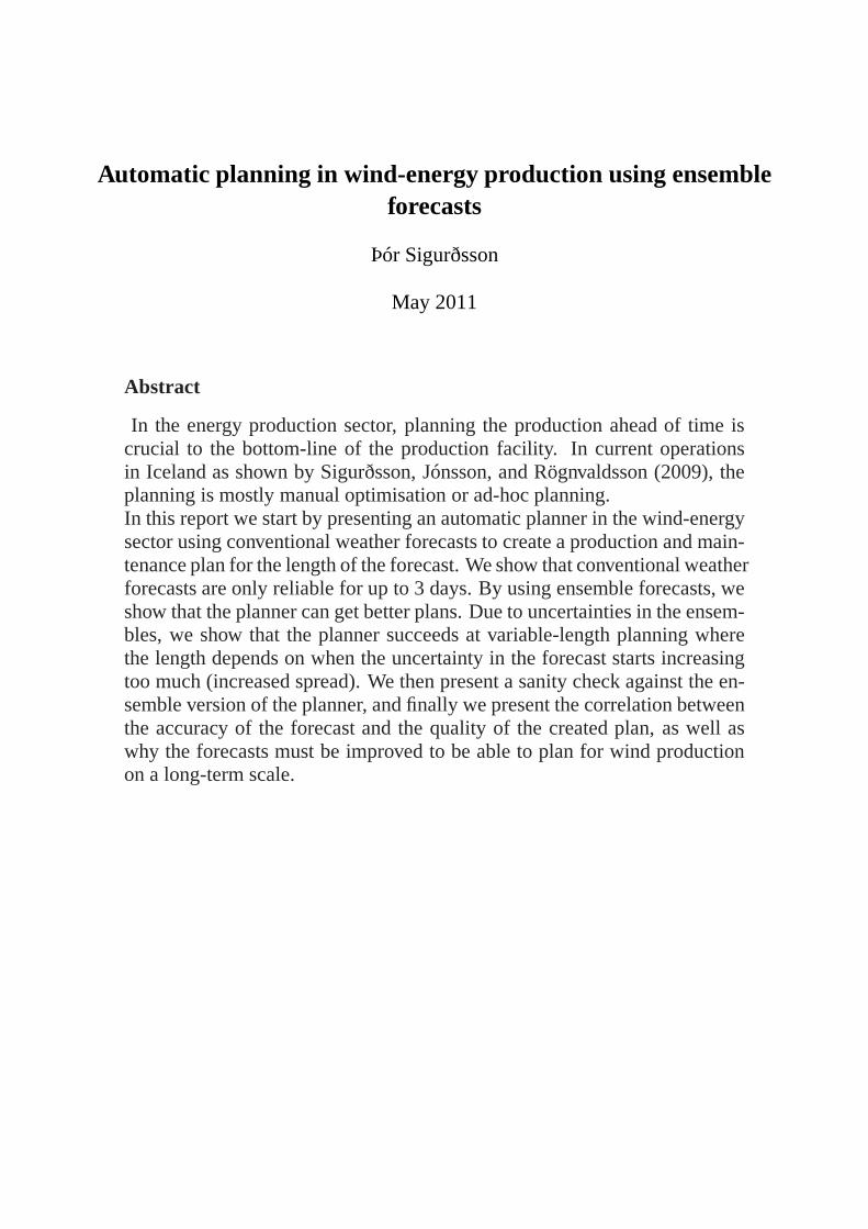
Abstract
In the energy production sector, planning the production ahead of time iscrucial to the bottom-line of the production facility. In current operationsin Iceland as shown by Sigurðsson, Jónsson, and Rögnvaldsson (2009), theplanning is mostly manual optimisation or ad-hoc planning.In this report we start by presenting an automatic planner inthe wind-energysector using conventional weather forecasts to create a production and main-tenance plan for the length of the forecast. We show that conventional weatherforecasts are only reliable for up to 3 days. By using ensemble forecasts, weshow that the planner can get better plans. Due to uncertainties in the ensem-bles, we show that the planner succeeds at variable-length planning wherethe length depends on when the uncertainty in the forecast starts increasingtoo much (increased spread). We then present a sanity check against the en-semble version of the planner, and finally we present the correlation betweenthe accuracy of the forecast and the quality of the created plan, as well aswhy the forecasts must be improved to be able to plan for wind productionon a long-term scale.

Sjálfvirk áætlanagerð í vindorkuframleiðslu með notkunklasaspáa
Þór Sigurðsson
Maí 2011
Útdráttur
Í orkuframleiðslugeiranum er mikilvægt fyrir framlegð virkjunarinnar aðgera framleiðsluáætlanir fram í tímann. Í núverandi framleiðsluferlum á Ís-landi, eins og sýnt er í Sigurðsson et al. (2009), er áætlanagerð að mestubyggð á línulegri bestun eða ad-hoc áætlanagerð.Í þessarri skýrslu byrjum við á að kynna sjálfvirka áætlanagerð í vindorkuverisem nýtir hefðbundnar tölvureiknaðar veðurspár til að búa til framleiðslu- ogviðhaldsáætlun eins langt og veðurspáin leyfir. Við sýnum aðhefðbundinveðurspá nýtist til áætlanagerðar allt að 3 daga fram í tímann. Með því aðnotast við klasaspár sýnum við fram á að hægt er að búa til betri áætlanir.Sökum óvissu í spánum sýnum við að áætlanagerðin ræður aðeins við áæt-lanir þar sem lengd spárinnar er upp að þeim tímapunkti þar sem óvissanverður of mikil í spánni (aukin dreifing). Við kynnum síðan prófun á áæt-lanagerðinni þar sem prófaður er klasapárhlutinn. Að lokumkynnum viðtengsl milli gæða spárinnar og nákvæmni áætlunarinnar og svo hversvegnaspárnar verða að verða betri til að áætlanagerð í vindorkugeiranum sé mögu-leg fyrir lengri tímabil.

Dedicated to my mother whose dedication to my studies is admirable.
Dedicated with love to for her caring and support.


vii
Acknowledgements
Dr. Ari Kristinn Jónsson for his mentoring and guidance in this project.
Ólafur Rögnvaldsson for providing a place of work and funding for this project as well as
his expertise and guidance.
Dr. Örnólfur E. Rögnvaldsson for his valued guidance, expertise and time.
Hálfdán Ágústsson and Einar Magnús Einarsson for their valued guidance.
Sara Sigurðardóttir for her valued assistance.

viii
ix
Contents
List of Figures xi
List of Tables xii
1 Introduction 1
2 Background and Motivation 3
2.1 Weather forecasting . . . . . . . . . . . . . . . . . . . . . . . . . . . . . 4
2.2 The Icelandic energy market, consumption estimation and power production 8
2.3 Automatic Planning Using AI . . . . . . . . . . . . . . . . . . . . . . . 9
3 Overview 11
4 Methods and Model 17
4.1 The Model . . . . . . . . . . . . . . . . . . . . . . . . . . . . . . . . . . 17
4.2 The Data converter . . . . . . . . . . . . . . . . . . . . . . . . . . . . . 18
4.3 The Planner / Runner . . . . . . . . . . . . . . . . . . . . . . . . . . . . 19
4.3.1 Determining if production will be available a state . .. . . . . . 20
4.3.2 The state machines . . . . . . . . . . . . . . . . . . . . . . . . . 22
4.3.3 Calculating resources . . . . . . . . . . . . . . . . . . . . . . . . 25
4.3.4 The Runner . . . . . . . . . . . . . . . . . . . . . . . . . . . . . 26
4.4 Postprocessing . . . . . . . . . . . . . . . . . . . . . . . . . . . . . . . 27
4.5 Heuristics, statistics and search methods . . . . . . . . . . .. . . . . . . 28
4.6 Variations on A∗ . . . . . . . . . . . . . . . . . . . . . . . . . . . . . . . 30
4.6.1 Improving time efficiency while keeping (most) of the search ac-
curacy . . . . . . . . . . . . . . . . . . . . . . . . . . . . . . . . 31
4.6.2 Optimistic and pessimistic planners . . . . . . . . . . . . . .. . 32
4.7 Baseline Testing . . . . . . . . . . . . . . . . . . . . . . . . . . . . . . . 34
5 Results 37

x
5.1 Planning against a conventional weather forecast . . . . .. . . . . . . . 37
5.2 Planning against an ensemble forecast . . . . . . . . . . . . . . .. . . . 38
6 Conclusions 45
Bibliography 47
A Appendix 51
A.1 The Planner . . . . . . . . . . . . . . . . . . . . . . . . . . . . . . . . . 51
A.1.1 The planner options . . . . . . . . . . . . . . . . . . . . . . . . . 51
xi
List of Figures
2.1 The three domains . . . . . . . . . . . . . . . . . . . . . . . . . . . . . . 4
2.2 Numerical weather models . . . . . . . . . . . . . . . . . . . . . . . . . 5
2.3 Evolution of ECMWF forecast skill . . . . . . . . . . . . . . . . . . .. 6
2.4 Location of weather station and model . . . . . . . . . . . . . . . .. . . 7
2.5 Airport at Kirkjubæjarklaustur . . . . . . . . . . . . . . . . . . . .. . . 8
3.1 The current state and path, proposed path . . . . . . . . . . . . .. . . . 12
4.1 The Model . . . . . . . . . . . . . . . . . . . . . . . . . . . . . . . . . . 18
4.2 The structure of the stored data in the database . . . . . . . .. . . . . . . 19
4.3 The state machine used in the planner . . . . . . . . . . . . . . . . .. . 23
4.4 The state machine used in the runner . . . . . . . . . . . . . . . . . .. . 24
4.5 Correlation between heuristics . . . . . . . . . . . . . . . . . . . .. . . 29
5.1 A plain Weather forecast and the correlation between measured and in-
terepreted values,x-axis is hours . . . . . . . . . . . . . . . . . . . . . . 38
5.2 Results of running the first four heuristics,x-axis is hours . . . . . . . . . 39
5.3 Mean value for grouped data - ensemble forecast vs. conventional fore-
cast,x-axis is hours . . . . . . . . . . . . . . . . . . . . . . . . . . . . . 40
5.4 Results from running with different confidence values,x-axis is hours . . 41
5.5 Confidence value at 60/100 with increased and the correlation between
interpreted and measured wind,x-axis is hours . . . . . . . . . . . . . . 42
5.6 The spread of the ensemble graphs for two periods - less spread is higher
confidence,x-axis is 6-hour steps . . . . . . . . . . . . . . . . . . . . . . 42
5.7 Results from Yamaguchi and Ishihara (2008) showing false positives and
false negatives . . . . . . . . . . . . . . . . . . . . . . . . . . . . . . . . 43
5.8 Early exit . . . . . . . . . . . . . . . . . . . . . . . . . . . . . . . . . . 44

xii

xiii
List of Tables
4.1 Database Declaration . . . . . . . . . . . . . . . . . . . . . . . . . . . . 19
4.2 Plant facts data structure . . . . . . . . . . . . . . . . . . . . . . . . .. 21
4.3 Transition table for state machine in planner - no wind . .. . . . . . . . 23
4.4 Transition table for state machine in planner - with wind. . . . . . . . . 23
4.5 The possible states of the planner . . . . . . . . . . . . . . . . . . .. . . 24
4.6 The States and the Actions possible in each state . . . . . . .. . . . . . . 25
4.7 Resource-Production-Consumption Legend . . . . . . . . . . .. . . . . 26
4.8 Planner/Runner output tables . . . . . . . . . . . . . . . . . . . . . .. . 27
4.9 Available heuristics/algorithms . . . . . . . . . . . . . . . . . .. . . . . 30
4.10 Tests of different depths of A∗-EC . . . . . . . . . . . . . . . . . . . . . 34

xiv

1
Chapter 1
Introduction
In energy production and sales, planning ahead is one of the most crucial elements in
operations. Energy sales are typically done ahead of time and thus energy producers must
guarantee the delivery of energy. If there is a change that makes a producer unable to
comply with production numbers promised, energy must be bought on a “spot market”,
at a price many times (up to 45 times the regular market price is not unusual (Landsnet
Spot-Market prices, 2011)) that of a planned purchase.
In Chapter 2 we present the background for this project and our motivation to do so.
In Chapter 3 we present a planner written for wind power plants with the notion of be-
ing able to make production and “maintenance” (recurrent events) plans as needed. We
then create plans against conventional weather forecasts.We show that the conventional
weather forecasts can support plans for up to 3 days, and thatthese forecasts are not the
best candidates for planning since they lack necessary quantitative information about the
uncertainty of the weather system. We show that by using ensemble forecasts we can pro-
duce better plans, as well as predict the quality of the forecasts, allowing us to selectively
plan for more certain periods, or stop the planner from planning further when the forecast
becomes too unreliable. In Chapter 4 we present the model andthe helper applications.
First we present an overview of the model. Next we describe the data converter used to
retrieve the weather forecasts, followed by a detailed description of the planner and runner
and its parts. Finally, we describe the baseline tests used to sanity-check the planner. In
Chapter 5 we present the results of the simulations where we show how well the heuristics
handle the planning, and especially how detrimental bad input data can be to the planner.
In Chapter 6 we present the conclusions of this research, as well as what is being done to
improve the ensemble forecasts beyond what they offer today.

2

3
Chapter 2
Background and Motivation
In 2008-2009, we did a research project for Reykjavik Energy(Orkuveita Reykjavíkur,
OR) Environment and Energy Research Fund (UOOR). In the project Sigurðsson et al.
(2009) we examined the state of the energy industry in Iceland, in particular with respect
to which methods were used in production planning.
Our findings were that where plans are created, a specialist uses manual optimization
based on the current state of the system (fed into an Excel model showing the trends
for the changes in the system) and a weather forecast which isinput into a flow model
(containing historical weather data 1985-2006 (Sigurðsson et al., 2009, p. 7)) to create
the plan. This manual approach limits severely what optionsmay be explored, since each
iteration is time consuming and only a single, or very few options may be examined.
Previously, conventional weather forecasts were used as input to the flow models, but
recently, ensemble forecasts have been used.
Previous work done in planning for complex projects, includes The Mars Rover project,
where Bresina, Jónsson, Morris, and Rajan (2005) created plans for extremely time-
sensitive and complex situations and presented in human-readable form for verification
and acceptance. The LORAX project, where Jónsson, McGann, Pedersen, Iatauro, and
Rajagopalan (2005) used automatic planning to create action plans in an autonomous
droid in Antartica. And the research on Short-Term Multiperiod Optimal Planning of
Utility Systems Using Heuristics and Dynamic Programming,where Kim and Han (2001)
used non-linear and dynamic programming to create plans forsteam-based power plants.
We considered the possibility of using automatic planning for creating production plans
for Icelandic power plants, using wind farms as our target since they are the most volatile
(giving us a chance of seeing results on a relatively short timeframe compared with
4 Automatic planning in wind-energy production using ensemble forecasts
geothermal or hydro power) and to see if we can improve the base results by using en-
semble forecasts which should provide us with the uncertainty measure we need.
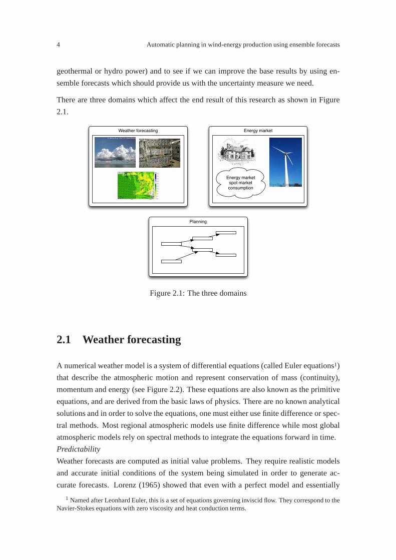
There are three domains which affect the end result of this research as shown in Figure
2.1.
Energy market
Energy marketspot marketconsumption
Weather forecasting
Planning
Figure 2.1: The three domains
2.1 Weather forecasting
A numerical weather model is a system of differential equations (called Euler equations1)
that describe the atmospheric motion and represent conservation of mass (continuity),
momentum and energy (see Figure 2.2). These equations are also known as the primitive
equations, and are derived from the basic laws of physics. There are no known analytical
solutions and in order to solve the equations, one must either use finite difference or spec-
tral methods. Most regional atmospheric models use finite difference while most global
atmospheric models rely on spectral methods to integrate the equations forward in time.
Predictability
Weather forecasts are computed as initial value problems. They require realistic models
and accurate initial conditions of the system being simulated in order to generate ac-
curate forecasts. Lorenz (1965) showed that even with a perfect model and essentially
1 Named after Leonhard Euler, this is a set of equations governing inviscid flow. They correspond to theNavier-Stokes equations with zero viscosity and heat conduction terms.
Þór Sigurðsson 5
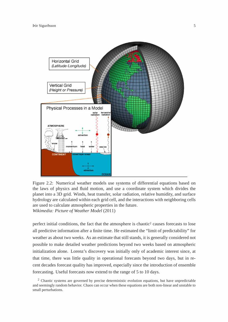
Figure 2.2: Numerical weather models use systems of differential equations based onthe laws of physics and fluid motion, and use a coordinate system which divides theplanet into a 3D grid. Winds, heat transfer, solar radiation, relative humidity, and surfacehydrology are calculated within each grid cell, and the interactions with neighboring cellsare used to calculate atmospheric properties in the future.Wikimedia: Picture of Weather Model(2011)
perfect initial conditions, the fact that the atmosphere ischaotic2 causes forecasts to lose
all predictive information after a finite time. He estimatedthe “limit of predictability” for
weather as about two weeks. As an estimate that still stands,it is generally considered not
possible to make detailed weather predictions beyond two weeks based on atmospheric
initialization alone. Lorenz’s discovery was initially only of academic interest since, at
that time, there was little quality in operational forecasts beyond two days, but in re-
cent decades forecast quality has improved, especially since the introduction of ensemble
forecasting. Useful forecasts now extend to the range of 5 to10 days.
2 Chaotic systems are governed by precise deterministic evolution equations, but have unpredictableand seemingly random behavior. Chaos can occur when these equations are both non-linear and unstable tosmall perturbations.
6 Automatic planning in wind-energy production using ensemble forecasts
Ensemble forecasts
In addition to imperfect initial condition, a second sourceof forecast error exists. The
imperfection of the atmospheric models themselves. These two sources of uncertainties
limit the usefulness of a single weather forecast. One way toovercome these problems
is to run many forecasts, instead of a single deterministic one, where initial conditions
have been nudged and/or the stochastic physics of the atmospheric model itself. This
way, an ensemble of forecasts is created from which a probability density function in the
atmosphere’s phase space can be determined for individual forecast parameters.
An overview of ensemble forecasting and ensemble data assimilation is given in Zhang
and Pu (2010). The usefulness of forecasts also depends on what weather parameter is in
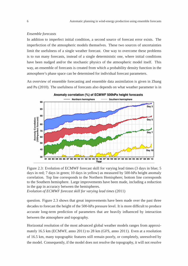
Figure 2.3: Evolution of ECMWF forecast skill for varying lead times (3 days in blue; 5days in red; 7 days in green; 10 days in yellow) as measured by 500-hPa height anomalycorrelation. Top line corresponds to the Northern Hemisphere; bottom line correspondsto the Southern hemisphere. Large improvements have been made, including a reductionin the gap in accuracy between the hemispheres.Evolution of ECMWF forecast skill for varying lead times(2011)
question. Figure 2.3 shows that great improvements have been made over the past three
decades to forecast the height of the 500-hPa pressure level. It is more difficult to produce
accurate long-term prediction of parameters that are heavily influenced by interaction
between the atmosphere and topography.
Horizontal resolution of the most advanced global weather models ranges from approxi-
mately 16.5 km (ECMWF, anno 2011) to 28 km (GFS, anno 2011). Even at a resolution
of 16.5 km, many topographic features still remain poorly, or completely, unresolved by
the model. Consequently, if the model does not resolve the topography, it will not resolve
Þór Sigurðsson 7
accurately the effects the topography has on the atmospheric flow. Due to this, it can be
very difficult to produce accurate wind forecasts in complextopography.
Weather forecasts are a set of estimates of variables (wind,precipitation, etc.) for a se-
lected area provided by an atmospheric model like WRF Skamarock et al. (2008) or MM5
Grell, Dudhia, and Stauffer (1995). In this paper, we do not consider weather forecast-
ing in detail and suffice with using output data from atmospheric models as input data
for our model. We use deterministic forecasts as well as ensemble forecasting to provide
estimates of the statistical distribution of future weather conditions. In our case, we use
the GFSNOAA GFS Webpage(2011) ensemble data provided by NCEP (National Center
for Environmental prediction). The ensemble consists of a deterministic forecast based
on a "true" analysis of the atmosphere and 20 additional forecasts that are based on initial
conditions that are slightly perturbed relative to the "true" analysis.
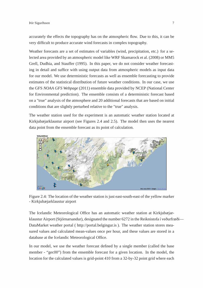
The weather station used for the experiment is an automatic weather station located at
Kirkjubæjarklaustur airport (see Figures 2.4 and 2.5). Themodel then uses the nearest
data point from the ensemble forecast as its point of calculation.
Figure 2.4: The location of the weather station is just east-south-east of the yellow marker- Kirkjubæjarklaustur airport
The Icelandic Meteorological Office has an automatic weather station at Kirkjubæjar-
klaustur Airport (Stjórnarsandur), designated the number6272 in the Reiknistofa í veðurfræði—
DataMarket weather portal ( http://portal.belgingur.is ). The weather station stores mea-
sured values and calculated mean-values once per hour, and these values are stored in a
database at the Icelandic Meteorological Office.
In our model, we use the weather forecast defined by a single member (called the base
member - “gec00”) from the ensemble forecast for a given location. In the model, the
location for the calculated values is grid-point 410 from a 32-by-32 point grid where each
8 Automatic planning in wind-energy production using ensemble forecasts
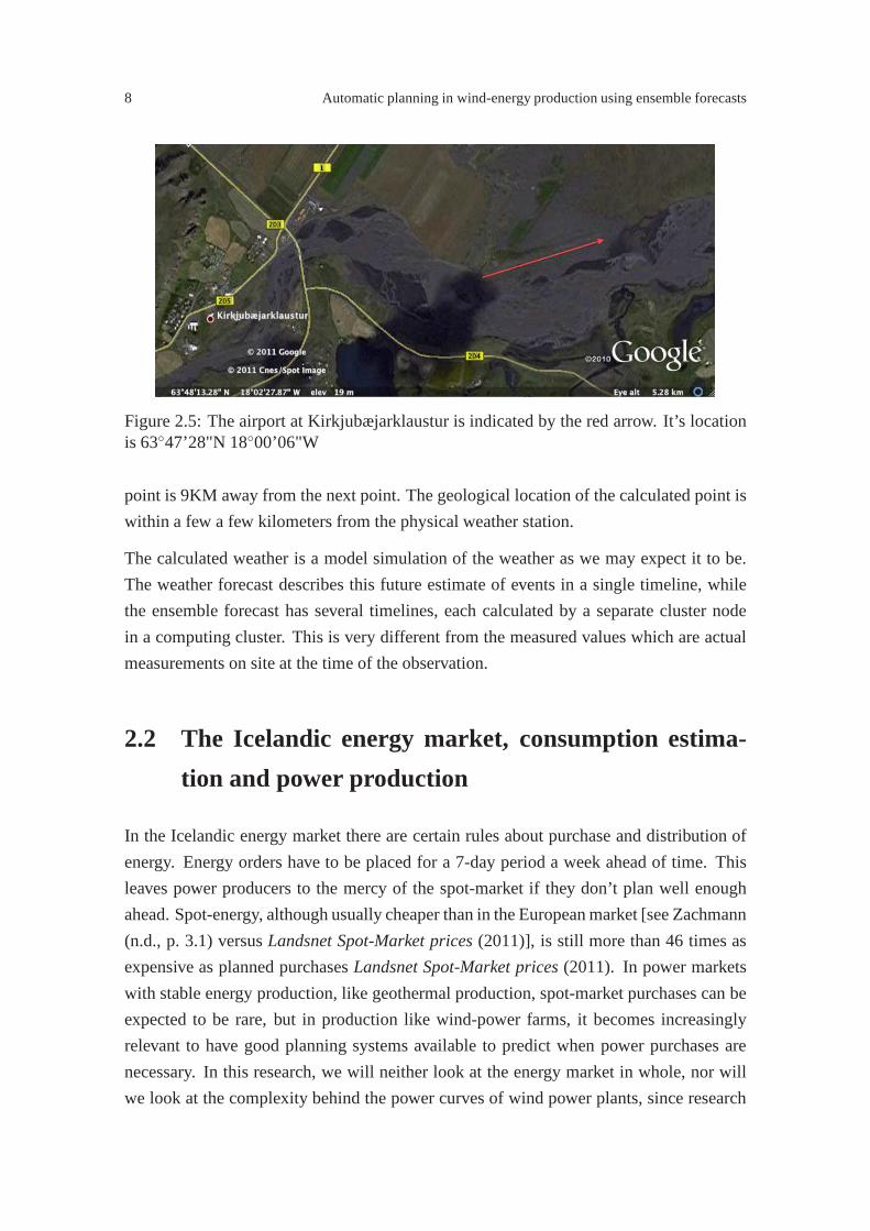
Figure 2.5: The airport at Kirkjubæjarklaustur is indicated by the red arrow. It’s locationis 63◦47’28"N 18◦00’06"W
point is 9KM away from the next point. The geological location of the calculated point is
within a few a few kilometers from the physical weather station.
The calculated weather is a model simulation of the weather as we may expect it to be.
The weather forecast describes this future estimate of events in a single timeline, while
the ensemble forecast has several timelines, each calculated by a separate cluster node
in a computing cluster. This is very different from the measured values which are actual
measurements on site at the time of the observation.
2.2 The Icelandic energy market, consumption estima-
tion and power production
In the Icelandic energy market there are certain rules aboutpurchase and distribution of
energy. Energy orders have to be placed for a 7-day period a week ahead of time. This
leaves power producers to the mercy of the spot-market if they don’t plan well enough
ahead. Spot-energy, although usually cheaper than in the European market [see Zachmann
(n.d., p. 3.1) versusLandsnet Spot-Market prices(2011)], is still more than 46 times as
expensive as planned purchasesLandsnet Spot-Market prices(2011). In power markets
with stable energy production, like geothermal production, spot-market purchases can be
expected to be rare, but in production like wind-power farms, it becomes increasingly
relevant to have good planning systems available to predictwhen power purchases are
necessary. In this research, we will neither look at the energy market in whole, nor will
we look at the complexity behind the power curves of wind power plants, since research

Þór Sigurðsson 9
in that area is plentiful (see e.g. Nielsen et al. (2006), Kimand Han (2001)) and is outside
the scope of the planning problems.
2.3 Automatic Planning Using AI
In todays demand for efficiency and return of investment (ROI), automatic planning is
being used more and more. It is being used in fields like the carindustry for production
lines, warehouses, the space industry and autonomous scientific applications. In light
of the results of the UOOR project, where it became apparent that automatic planning
was not being used in the Icelandic energy production sector, and the success of using
automatic planning in complex systems like the Mars Rover and Lorax, we saw an op-
portunity to see if planning could indeed be used in the energy production sector. Since
we also have access to the meteorology sector, we have interest in seeing if the current
practices can be improved, and if by using better forecasts,we could improve the planning
even further.

10
11
Chapter 3
Overview
In 2008-2009 we conducted research for the Environment and Energy Research Fund
Sigurðsson et al. (2009) where we examined the main Icelandic energy producers and
their environment, looking for areas which would be affected by environmental factors
and how automatic planning might help in solving the problems the producers might face.
While conducting this research it became apparent that automatic planning wasn’t being
used at all. There were a number of questions raised.
When exmining work already done in the field of ensemble forecasts and power plants,
work done by Nielsen et al. (2006) presents a method of converting the ensemble wind
metrics to an estimated power output of a wind farm and Yamaguchi and Ishihara (2008)
adds to that a multi-timescale parameter. Although Nielsenet al. (2006) do not use auto-
matic planning, their method may be used as an intermediate step in this model to convert
the wind metrics directly to power curve metrics. It has however for the purpose of this
research, been chosen not to implement it since it will complicate the model and will
have little if any effect on the results. No references were found on the use of automatic
planning using ensemble forecasts in wind-energy production, but one company,Garrad-
Hassan Webpage(2011), may have implemented such planning without releasing public
information about it.
The current state of the art in the Icelandic power production planning involves getting
metrics through measurements and manually weighing them against a perceived best solu-
tion based on subjective professional experience. In situations where uncertainty is high,
the time to find an acceptable solution may be long and the solution chosen may be far
from the best available. Factored into the selection process are recurrent events like regu-
lar maintenance, planning in what might be unforseen events(like distribution flaws due

12 Automatic planning in wind-energy production using ensemble forecasts
to weather, failing distribution system, etc.), coordination of several power plants each
different from others and each with its own recurrent events.
The planning/atmospheric model combination can be illustrated as in Figure 3.1. The
state of the art, marked by the mark on the left, is moving in the direction of the solid line.
This research will look into the use of automated planning instead of manual optimisation
and whether such a solution does better by using ensemble forecasts, as signified by the
broken line.
Figure 3.1: The current state and path, proposed path
The focus
In this research, we will use a wind power plant as our target.
The choice of a wind power plant is based on two factors
• The simplicity of the wind power plant parameters and the possibility of simplifying
the model without losing relevant accuracy
• The short-term nature of wind forecasts1
In this research, we will answer the following two questions, and describe our find-
ings:
• Can we use an automatic planner to plan for a wind power plant using conventional
weather forecasts?
• If we replace the conventional forecast with an ensemble forecast, do we get better
results?
To which the answers are:
• We can use an automatic planner to plan for a wind power plant on a short term basis
(up to 3 days), but on a long term base it will not be helpful to use conventional
1 Since direct effects of weather on hydro and geothermal power plants can be expected to be primarilyof long-term nature, the direct dependence of production inwind power plants on weather was deemedmore relevant for examining the effectivness of a planner for power production systems, as well as forinvestigating the qualitative difference between ensemble forecasts and traditional weather forecasts

Þór Sigurðsson 13
weather forecasts since there is no quantitative information in the forecast to tell
about the quality of the forecast itself which may in turn derail the plan.
• If we replace the conventional forecast with an ensemble forecast, it will provide
us with better results. It is not quite on the scale we expected. The base range is
still up to 3 days, but we now have the benefit of actually beingable to track some
forecasts for a longer time with higher confidence than we could in the conventional
forecast, since the ensembles work as a measure on the uncertainty of the forecast,
and therefore on the quality and probability of the outcome.The ensemble forecasts
may also be used to find periods of certainty in the timeframe and create plans
for these, even if there is a large uncertainty on both ends (that is, given a period
of uncertainty, if we have a period at the end of that which all/mosts members
of the ensemble agree upon, we can plan for that part even if wecan’t plan for
the preceding uncertainty). That means we can maken partial plans for the given
period and end up with a set of plans that may aid us through in the best fashion
possible, considering the lack of a complete plan. The problem is however that the
ensemble data does not present us with a profile of the wind system in fine enough
granularity for us to predict with any certainty how the weather system will behave
beyond a “mean value” (10-minute mean wind in a 6-hour period). In Chapter 6,
we present suggestions to what needs to be examined next in terms of improving
the ensemble forecasts in such a way that they may prove beneficial to the wind
power production industry.
If we are able to show that automatic planning in wind power production systems is pos-
sible using the methods we propose, then these methods may beapplied to other temporal
systems like hydropower and geothermal power, both of whichare more stable systems
than wind power, with at least equal long-term benefits. Since the weather model for hy-
dropower and geothermal power plants changes less rapidly and with fewer variations than
the wind model, and as such, long-term planning may be of evenbigger benefit on a larger
(national) scale, while the wind power will show benefits on ashort-term scale.
The second question comes into play on the quality of the plans. For the producer, this
is important since a plan needs to be very accurate if it is going to keep the producer in
positive productivity. Once the plan accuracy drops below agiven percentage (depending
on time of day and year since spot-market prices fluctuate greatly), the producer becomes
less of a producer and more of an energy reseller. When running our simulations, we esti-
mated a spot-market price of 4x the standard purchace price.That implies a plan accuracy
of approximately 80% (not taking into account that the producer may sometimes sell into
the spot-market as well). Since the experiements were done,Landsnet has updated their
14 Automatic planning in wind-energy production using ensemble forecasts
website, publicing actual historical data on spot-market prices as well as current market
prices. This newly publicized information suggests that weunderestimated the highest
spot-market prices 12-fold and overestimated the lowest spot-market prices 2-fold. This
information was not available when the system was written.
Automatic planning using AI
In automatic planning there are many diverse planning methods available, each with its
own merits. Planning based on a temporal datastream like a weather forecast is a fixed
depth search problem. We have a fixed number of steps our plan must have (the number
of time steps in the weather model in the base case, and the number of steps there are
from the start of the plan until the uncertainty of forecast becomes too great - in either
case, the number between the end-points is fixed, that is – we cannot add or omit any steps
to/from the data stream). The implementation of the plannerrequires us to implement a
problem area that represents the recurrent issues that trouble the energy industry in one
way or another, like maintenance, fluctuations of other energy production facilities and
even recurrent weather-connected events. We chose to implement one recurrent event per
production plant where an event had to occur within a certainwindow of opportunity.
This window of opportunity is then reset so the event has to take place again. We call the
event “maintenance”, but in reality it can take place of any time-sensitive recurrent event
as needed. The presence of the recurrent event means we cannot use linear optimization
to create a plan for our facility. Since the problem is a sequential temporal problem, we
claim that a search (e.g. A∗ 2 Russell and Norvig (2003)), with some modifications to
make it more benign in terms of speed and resource usage, willsuffice to find the best
plan.
In the planner we test a variety of heuristics, where the differences between heuristics have
to do with the way we interpret the ensemble data. Since thereis an arbitrary number
of members in the ensemble, and they are not necessarily sequential (since a member
may fail in its attempt to create the forecast), several interpretations of the ensembles are
attempted and found to give suboptimal results - midvalue and midrange, the mean for
grouped data, the modal for grouped data Bluman (2008), fitting the baseline to the trend
in the ensemble and finally the confidence level of the ensemble (where we check if a
certain percentage of the members land within the set production range) with and without
a deviation check for early exit.
When purchasing energy, an estimate is created on an hourly basis for a full week - both
for production and consumption. All failures in production(energy already sold but not
produced) have to be purchased and this is done through energy wholesale retailers. While
2 A∗ is a tree-based search method which can be applied in planning problems

Þór Sigurðsson 15
it is essential for the company to create such purchase plans, productionmayfail (due to
malfunctions, lack of resources etc.) and when that happens, the company must purchase
the energy on a spot market at a price over four times the regular purchase price (depend-
ing on supply and demand). The producer of energy benefits from good planning as he
may conduct maintenance when production would otherwise beat a low.
As we show in Chapter 5, we find that planning for wind production using conventional
weather forecasts works somewhat well for a up to 3 days. Longer periods are however
affected by the forecast diverging from the real weather, causing the plan to fail due
to the input data. When upgrading to ensemble forecasts, we show that the planning
period does in many cases extend itself further than the 3 days of the conventional weather
forecast, it handles better than the conventional forecastin terms of being able to see
when the uncertainty is low, and create plans for those periods, and bail out on periods
where uncertainty is very high, thus not wasting resources on plans that cannot with any
guarantee hold against the real world.
We also perform a basline test on the planner to sanity test the plannning functions.

16

17
Chapter 4
Methods and Model
In this chapter, we start by giving an overview of the model that the planning process
operates within. We then go on to describe the tools we created to handle the data and the
planner and the variations that we have tested in this research.
4.1 The Model
The model is a description of a wind-power plant consisting of 0 < n ≤ 6 windmills,
a repository (batteries) for short-term energy storage, a definition of recurrent events
(“maintenance”), a consumption of energy and a weather system as shown in Figure 4.1.
Consumption in the model is preset at 12MW per hour. The production capability is
user settable per windmill as are the repositories and maintenance periods of each wind-
mill. The weather system consists of data from the environmental weather model WRF
(Skamarock et al., 2008) which creates weather forecasts for a region based on initial and
boundary conditions. Part of the boundary conditions are static (i.e. the terrain maps)
while atmospheric boundary and initial conditions come from global atmospheric mod-
els, in our case the GFS (NOAA GFS Webpage, 2011) model. In addition to the simulated
weather from the forecasting model, observational data fora specific location was used in
the runner phase. For this purpose, measured data for a location within the ensemble grid
was acquired from the Icelandic Meterological Office. The observational measurements
cover 1477 hourly measurements.
18 Automatic planning in wind-energy production using ensemble forecasts
Weather Forecasts
Ensemble Forecasts
Measured weather
conditions
Planner Runner
Financial state
Weather model
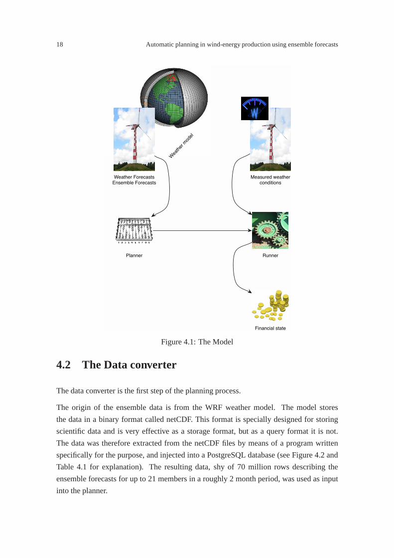
Figure 4.1: The Model
4.2 The Data converter
The data converter is the first step of the planning process.
The origin of the ensemble data is from the WRF weather model.The model stores
the data in a binary format called netCDF. This format is specially designed for storing
scientific data and is very effective as a storage format, butas a query format it is not.
The data was therefore extracted from the netCDF files by means of a program written
specifically for the purpose, and injected into a PostgreSQLdatabase (see Figure 4.2 and
Table 4.1 for explanation). The resulting data, shy of 70 million rows describing the
ensemble forecasts for up to 21 members in a roughly 2 month period, was used as input
into the planner.
Þór Sigurðsson 19
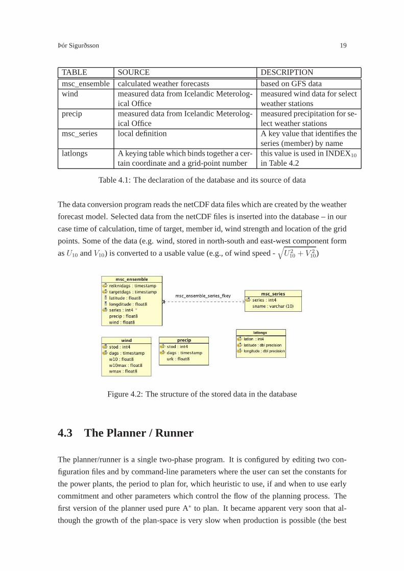
TABLE SOURCE DESCRIPTION
msc_ensemble calculated weather forecasts based on GFS datawind measured data from Icelandic Meterolog-
ical Officemeasured wind data for selectweather stations
precip measured data from Icelandic Meterolog-ical Office
measured precipitation for se-lect weather stations
msc_series local definition A key value that identifies theseries (member) by name
latlongs A keying table which binds together a cer-tain coordinate and a grid-point number
this value is used in INDEX10in Table 4.2
Table 4.1: The declaration of the database and its source of data
The data conversion program reads the netCDF data files whichare created by the weather
forecast model. Selected data from the netCDF files is inserted into the database – in our
case time of calculation, time of target, member id, wind strength and location of the grid
points. Some of the data (e.g. wind, stored in north-south and east-west component form
asU10 andV10) is converted to a usable value (e.g., of wind speed -√
U210 + V 2
10)
Figure 4.2: The structure of the stored data in the database
4.3 The Planner / Runner
The planner/runner is a single two-phase program. It is configured by editing two con-
figuration files and by command-line parameters where the user can set the constants for
the power plants, the period to plan for, which heuristic to use, if and when to use early
commitment and other parameters which control the flow of theplanning process. The
first version of the planner used pure A∗ to plan. It became apparent very soon that al-
though the growth of the plan-space is very slow when production is possible (the best
20 Automatic planning in wind-energy production using ensemble forecasts
plan is easy to find since production always gives the best result — the real problem be-
comes selecting the timing of the maintenance periods) the plan-space grows by4d when
no production is possible, since all other possibilities atthe same and previous level in the
search tree become candidates once a counter–productive choice has to be made.
To counter this growth, the next iteration of the planner hadthe possibility of planning
only a few (user-selectable number of) steps (early commitment), commiting to the plan
and continue searching from that point on an equal number of steps. That ment that a
plan of 360 hours could e.g. be planned in 10 segments of 36 steps - or 36 segments of
10 steps. The growth problem was however still in the plannerand even 10-step searches
through a time serie with no possible production led to search times far exceeding the
actual period being searched.
This lead to the third iteration of the planner where early commitment was added. The
early commitment works by keeping a count of how many nodes have been expanded
and once the set amount has been reached, the planner examines the current node being
expanded, takes note of its level and goes upn levels in the tree (user selectable). In this
previous level, the best node is selected -both from the OpenList and ClosedListfor the
particular selected level, since the best node is very likely to have already been expanded.
The planner then commits to this node as the best solution, purges the OpenList and re-
sumes planning from that point in time. This method solved the growth problem in the
n-step early commitment planner described above. Care must however be taken that if
a too small number of nodes is set as early commitment – or too large backtracking of
levels — a loop may be created when the planner backs up to the source of the expansion
problem. A problem with early commitment may arise if the planner commits to a period
where nothing is done when it should commit to maintenace where a future production
may be compromised by a bad early commitment. This may be countered by examining
the plan structure and not allowing early commitment to commit to the last step before
production.
4.3.1 Determining if production will be available a state
The wind strength is the determining factor, as well as the previous state the windmill is
in. Since it does take some amount of time to start up the windmill as well as to shut it
down, this is simulated in the decision process by separate states with their own action
sets. We store information about the production plant in a data structure like the one
defined by Table 4.2. The data structure is the set of initial values for the power-plant, and
should be considered constant. It is only used in initializing the first state of the search
tree.

Þór Sigurðsson 21
INDEX Name Description
00 type Plant Type (0=wind, 1=water, . . . )01 genprodcap Production Capacity in % (0-1)02 maxprodcap Production Capacity in MW03 serviceinterval Maximum interval in timesteps04 servicestoplength Number of timesteps each service
interval must last05 startupprodcap Production capacity in % for the
startup phase06 shutdownprodcap Production capacity in % for the
shutdown phase07 res_max Maximum allowed storage of re-
serve power08 res_min Minimum allowed storage of re-
serve power09 res_lvl Current storage level of reserve
power10 location (DataPoint) The grid-location of the power plant. . . Reserved Reserved (not used)18 prod_above Production Trigger (Lower Bound)19 prod_below Production Trigger (Upper Bound)
Table 4.2: The data structure that stores facts about the power plant
All the σn variables are such thatn is the index to Table 4.2.
These are the formulae for wind production (a1 is the previous action anda2 is the current
one,ξ is the estimated/measured wind strength):
Calculate the MW multiplier to use if there is wind available:
ι1 = (σ18 ≤ ξ ≤ σ19)σ1σ2 (4.1)
Calculate the MW multiplier to use if there is no wind available:
ι2 = ((σ18 < ξ) ∨ (ξ > σ19))σ1σ2 (4.2)
If there’s wind:
P = ι1(a1 ∧ 3)(a2, 4)σ6 + ι1(a1, 2)(a2, 4)σ6
2+ ι1(a2, 3) + ι1(a2, 2)σ5 (4.3)
22 Automatic planning in wind-energy production using ensemble forecasts
And if there’s none:
P = ι2(a2, 4)σ6 (4.4)
For ι1 and ι2 in Equations 4.1 and 4.2, we check if the wind (ξ) is within the produc-
tion boundaries (σ18 . . . σ19) and them multiply it with the general production capabil-
ity (σ1, current capability,0 . . . 1) and maximum production capability (σ2, megawatts,
> 0).
For P , if there’s wind, only one of the four segments in Equation 4.3 will return a value
(since the logical-and creates a multiply-by-zero condition). Thea1 anda2 variables of
the formula define the current action (a2) and the previous action (a1) of the state machine
(see Section 4.3.2). The checks for actions and/or action-pairs return a value, 0 or 1. This
value is multiplied withι1/ι2 and then with a variable representing the production value
for said situation (e.g.σ6 for production under shutdown)
The value ofP is then used to evaluate the “quality” of the state (the production of energy
under the estimated or observed circumstances).
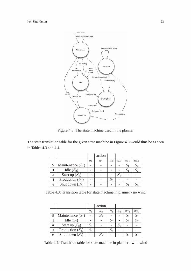
4.3.2 The state machines
Both the planners and the runners selection process are based on state machines. These
state machines control what actions are available at any given state, based on the weather
(for the planner) and based on the previous action taken, along with conditions given
by the resource calculation formula presented in Section 4.3.3. The state machine for the
planner is shown in Figure 4.3, and the transition table is shown in Tables 4.3 and 4.4. The
planner is a Finite State Machine (FSM). If there is too little wind to allow production, the
number of options available as actions to leave the state arereduced to the set indicated
by the broken lines. If there is wind, the number of actions isrepresented both by the
broken lines as well as the solid lines. From the options available the planner chooses an
action to take, based on the heuristic (see Section 4.5).
The method used to implement the state machine is similar to that of the Europa plan-
ning system written by NASA (EUROPA pso Platform for AI Planning, Scheduling, Con-
straint Programming and Optimization(2011)). That is, the state machine is defined and
designed before-hand, and then converted to a translation table where we can translate the
knowledge of the current state to an action that leads to a newstate.
Þór Sigurðsson 23
Maintenance
Idle
Starting Up
Producing
Shutting Down
Startup (σ5)
Start up (σ6)
Start up (σ5)
Shut down ((σ6)/2)
Produce (σ1σ2)
Keep producing (σ1σ2)
Shut down (σ6)
Do nothing (0)
Do maintenance (-p)
Keepdoing
nothing
Do nothing
Domaintenance
Keep doing maintenance
Figure 4.3: The state machine used in the planner
The state translation table for the given state machine in Figure 4.3 would thus be as seen
in Tables 4.3 and 4.4.
actiona1 a2 a3 a4 aε1 aε2
S Maintenance (S1) - - - - S1 S2
t Idle (S2) - - - - S1 S2
a Start up (S3) - - - S5 - -t Production (S4) - - S5 - - -e Shut down (S5) - - - - S1 S2
Table 4.3: Transition table for state machine in planner - nowind
actiona1 a2 a3 a4 aε1 aε2
S Maintenance (S1) - S3 - - S1 S2
t Idle (S2) - - S3 - S1 S2
a Start up (S3) S4 - - S5 - -t Production (S4) S4 - S5 - - -e Shut down (S5) - S3 - - S1 S2
Table 4.4: Transition table for state machine in planner - with wind
24 Automatic planning in wind-energy production using ensemble forecasts
e.g. in a given stateS4 (production), the planner takes an action depending on the heuristic
and the weather. In stateS4 according to the transition table for no wind (Table 4.3), in
stateS4 we have the only option ofa3, since that is the only action that provides a state
transition. That is, regardless of the heuristic, if there is no wind to power the turbine,
and the turbine was in a production phase, it will transitionto the shutdown phase which
returns the valueσ6. However, if there is wind, according to Table 4.4, in stateS4 we have
the option ofa1 (keep producing) anda3 (shutdown). The heuristic would provide which
action would be preferable.
Main-tenance
Idle
Shutting down
Producing
Startingup
Main-tenance
Idle
Shutting down
Producing
Startingup
Keep doing maintenance
Keepdoingnothing
Domaintenance
Donothing
Domaintenance
Do nothing
Shutdown
Shut down
Domaintenance
Donothing
Startup Shut
down
Shut down
Produce
Keepproducing
StartupDo
nothing
Domaintenance
Keepdoingnothing
Keep doing maintenance
Startup
If there is windIf there is no wind
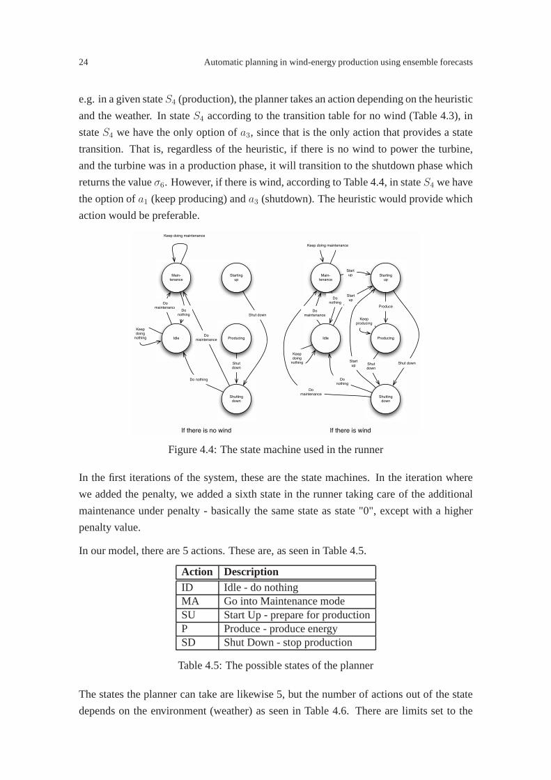
Figure 4.4: The state machine used in the runner
In the first iterations of the system, these are the state machines. In the iteration where
we added the penalty, we added a sixth state in the runner taking care of the additional
maintenance under penalty - basically the same state as state "0", except with a higher
penalty value.
In our model, there are 5 actions. These are, as seen in Table 4.5.
Action DescriptionID Idle - do nothingMA Go into Maintenance modeSU Start Up - prepare for productionP Produce - produce energySD Shut Down - stop production
Table 4.5: The possible states of the planner
The states the planner can take are likewise 5, but the numberof actions out of the state
depends on the environment (weather) as seen in Table 4.6. There are limits set to the
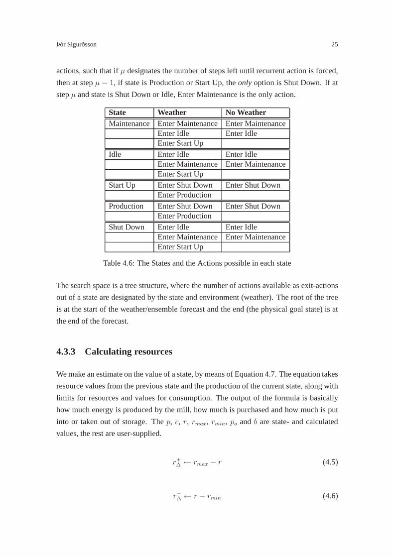
Þór Sigurðsson 25
actions, such that ifµ designates the number of steps left until recurrent action is forced,
then at stepµ − 1, if state is Production or Start Up, theonly option is Shut Down. If at
stepµ and state is Shut Down or Idle, Enter Maintenance is the only action.
State Weather No WeatherMaintenance Enter Maintenance Enter Maintenance
Enter Idle Enter IdleEnter Start Up
Idle Enter Idle Enter IdleEnter Maintenance Enter MaintenanceEnter Start Up
Start Up Enter Shut Down Enter Shut DownEnter Production
Production Enter Shut Down Enter Shut DownEnter Production
Shut Down Enter Idle Enter IdleEnter Maintenance Enter MaintenanceEnter Start Up
Table 4.6: The States and the Actions possible in each state
The search space is a tree structure, where the number of actions available as exit-actions
out of a state are designated by the state and environment (weather). The root of the tree
is at the start of the weather/ensemble forecast and the end (the physical goal state) is at
the end of the forecast.
4.3.3 Calculating resources
We make an estimate on the value of a state, by means of Equation 4.7. The equation takes
resource values from the previous state and the production of the current state, along with
limits for resources and values for consumption. The outputof the formula is basically
how much energy is produced by the mill, how much is purchasedand how much is put
into or taken out of storage. Thep, c, r, rmax, rmin, po andb are state- and calculated
values, the rest are user-supplied.
r+∆ ← rmax − r (4.5)
r−∆ ← r − rmin (4.6)

26 Automatic planning in wind-energy production using ensemble forecasts
Legend Description
p Productionc Consumptionrmax Maximum allowed reservoir levelrmin Minimum allowed reservoir levelr Reservoir levelr+∆ Difference betweenr andrmax
r−∆ Difference betweenr andrmin
po Overproduction (after consumption and reservoir)b Purchased (bought) energy (after insufficient reservoir and production)
Table 4.7: Resource-Production-Consumption Legend
Resource calculation formula:
c ≥ p⇒ c← c− p; p← 0;
r−∆ ≥ c⇒ r ← r − c; c← 0
r−∆ < c⇒ c← c− r−∆; r ← rmin; b← c; c← 0
c < p⇒ p← p− c; c← 0;
p ≥ r+∆ ⇒ r ← rmax; po ← p− r+
∆; p← 0
p < r+∆ ⇒ r ← r + p; p← 0
(4.7)
Equation 4.7 along with Equations 4.5 and 4.6 describes a setof requirements for the
value function when calculating resource usage;c is the consumption,p is the production
and so on (see Table 4.7).
The goal of the formula is to leave us with how much must be purchased, how much is
overproduction, how much is saved for later and how much is taken from reservoirs.
4.3.4 The Runner
The second phase of the program (the runner) takes the plan which was created in the first
phase and runs the plan on actual measured meteorological data.
Once the runner has read the plan and executed it against actual measure weather, both
the plan and the result are output in tabular form.
The output of the planner is twofold. Internally in the program, the return of the planner
is a list of plan actions which the runner then can utilise to perform its task. Externally
however, a table is printed in human-readable form. The columns of the planner output
are shown in Table 4.8.
In the runner, the only output is in machine-readable form (internally). The output is then
converted to human readable form on standard-out at the end of the run. The columns

Þór Sigurðsson 27
INDEX () Description
00 line number01 step number02 action taken in this step03 action taken in previous step04 node-ID05 previous node-ID06 produced energy07 purchased energy08 Not used09 reservoir status10 Not used11 Not used12 total value13 state value14 maintenance countdown 115 maintenance countdown 216 maintenance countdown 317 maintenance countdown 418 maintenance countdown 5 / debug item19 maintenance countdown 6 / debug item20 debug item21 wind (min value < current value < max value)
Table 4.8: Planner/Runner output tables
of the runner output are the same as those of the planner, except that there is no debug
output.
4.4 Postprocessing
Postprocessing is done by taking the output data from the planner/runner and convert it to
graphs using shell scripts and gnuplot/matplotlib.
The log files are copied from the host running the simulation,and are split into separate
logfiles for the plan and run. Then, from each set, the value columns (planned and actual),
wind (measured and estimated), action and planned action are collected into graphable
data files.
Once this is done, each dataset is plotted based on the specific features each graph is
intended to have (see the three main types of graphs used). Then, finally, a PDF is created,
containing all the graphs.
28 Automatic planning in wind-energy production using ensemble forecasts
4.5 Heuristics, statistics and search methods
A heuristic is a value function with wich we measure the distance to our goal. In A∗, the
heuristic is the h(n) part of the value function f(n)=g(n)+h(n). The function g(n) is the
value of the current state and h(n) is the heuristic (estimated future value).
In the planner we tried a variety of value functions. The value functions break up into
three parts. These are:
• Weather evaluation
We need to take the input from the weather forecast and somehow evaluate the
state. In conventional weather forecasts, the evaluation is done by evaluating the
wind strength against min and max values for the production curve of the wind
turbine. In ensemble forecasts we use the same evaluation, but before that, we
use the ensembles to get an estimate of what might be the rightvalue. In weather
applications, the midvalue is commonly used, so it was natural for us to start with
the midvalue and other statistical methods like it (λ0...3 as shown in Table 4.9). We
then gradually added others like the confidence level and early exit. As can be seen
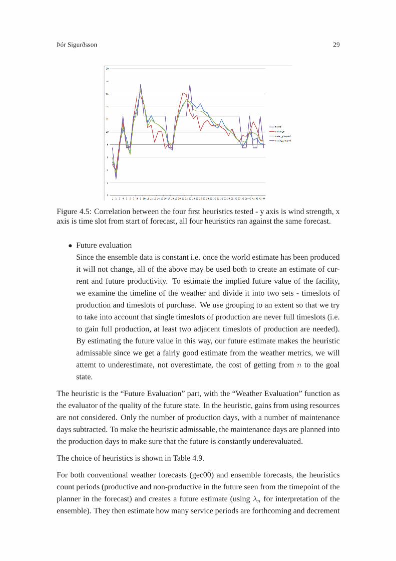
in Figure 4.5, the four metrics are very close in their estimate of the wind strength
based on the outcome of the members of the ensemble forecast.That means that of
the four metrics, it makes little difference which one we choose – we need to add
other elements to improve our estimate since a wrong estimate from any of the four
metrics will have the same incorrect effect on the distance estimate as any of the
other three.
We then added a confidence level – instead of examining what the actual wind
strength value was estimated at, we examined how many of the members said that
production would be within the range defined by the wind turbine as production
range. By tuning the confidence level we can affect how optimistic or pessimistic
the planner is. It turns out that the planner is less optimistic than before while having
a slightly better correlation between production estimates and actual production.
Lastly we add an early exit so that the planner exits the planning phase when the
ensemble forecasts become too erratic. This means that plans are generally much
shorter than the timespan of the weather forecast, but instead we have a plan that we
have more trust in, rather than one that covers forecasts with too high uncertainty.
• Resource usage
The power plant may or may not be defined with resources (batteries). The re-
sources must be considered both for underproduction as wellas overproduction.
Þór Sigurðsson 29
Figure 4.5: Correlation between the four first heuristics tested - y axis is wind strength, xaxis is time slot from start of forecast, all four heuristicsran against the same forecast.
• Future evaluation
Since the ensemble data is constant i.e. once the world estimate has been produced
it will not change, all of the above may be used both to create an estimate of cur-
rent and future productivity. To estimate the implied future value of the facility,
we examine the timeline of the weather and divide it into two sets - timeslots of
production and timeslots of purchase. We use grouping to an extent so that we try
to take into account that single timeslots of production arenever full timeslots (i.e.
to gain full production, at least two adjacent timeslots of production are needed).
By estimating the future value in this way, our future estimate makes the heuristic
admissable since we get a fairly good estimate from the weather metrics, we will
attemt to underestimate, not overestimate, the cost of getting from n to the goal
state.
The heuristic is the “Future Evaluation” part, with the “Weather Evaluation” function as
the evaluator of the quality of the future state. In the heuristic, gains from using resources
are not considered. Only the number of production days, witha number of maintenance
days subtracted. To make the heuristic admissable, the maintenance days are planned into
the production days to make sure that the future is constantly underevaluated.
The choice of heuristics is shown in Table 4.9.
For both conventional weather forecasts (gec00) and ensemble forecasts, the heuristics
count periods (productive and non-productive in the futureseen from the timepoint of the
planner in the forecast) and creates a future estimate (using λn for interpretation of the
ensemble). They then estimate how many service periods are forthcoming and decrement
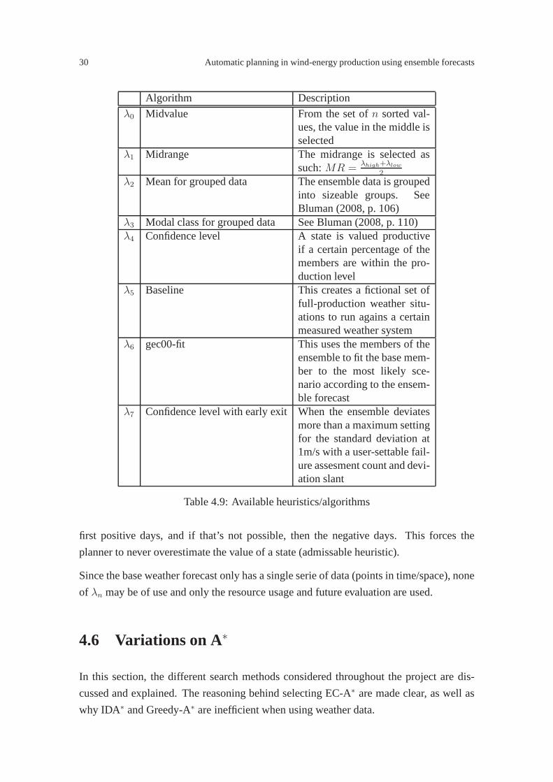
30 Automatic planning in wind-energy production using ensemble forecasts
Algorithm Description
λ0 Midvalue From the set ofn sorted val-ues, the value in the middle isselected
λ1 Midrange The midrange is selected assuch:MR =
λhigh+λlow
2
λ2 Mean for grouped data The ensemble data is groupedinto sizeable groups. SeeBluman (2008, p. 106)
λ3 Modal class for grouped data See Bluman (2008, p. 110)λ4 Confidence level A state is valued productive
if a certain percentage of themembers are within the pro-duction level
λ5 Baseline This creates a fictional set offull-production weather situ-ations to run agains a certainmeasured weather system
λ6 gec00-fit This uses the members of theensemble to fit the base mem-ber to the most likely sce-nario according to the ensem-ble forecast
λ7 Confidence level with early exit When the ensemble deviatesmore than a maximum settingfor the standard deviation at1m/s with a user-settable fail-ure assesment count and devi-ation slant
Table 4.9: Available heuristics/algorithms
first positive days, and if that’s not possible, then the negative days. This forces the
planner to never overestimate the value of a state (admissable heuristic).
Since the base weather forecast only has a single serie of data (points in time/space), none
of λn may be of use and only the resource usage and future evaluation are used.
4.6 Variations on A∗
In this section, the different search methods considered throughout the project are dis-
cussed and explained. The reasoning behind selecting EC-A∗ are made clear, as well as
why IDA∗ and Greedy-A∗ are inefficient when using weather data.

Þór Sigurðsson 31
4.6.1 Improving time efficiency while keeping (most) of the search
accuracy
Although the greedy algorithm of A∗ will be providing the best result within the bounds
of the heuristic, it will still, under circumstances out of the control of the user, expand mil-
lions and millions of nodes. In testing, at depth 10 it had already expanded over 2 million
nodes. The problem with A∗ is however that its growth rate is in the worst casebd (where
b is the number of options at each point in time at any given branch in the search tree, and
d is the depth of the search tree - in our case the number of time steps), which quickly be-
comes very large as A∗ keeps track of all expanded states — it quickly becomes memory
bound. Since the possible number of nodes isbd 1, the search space is prohibitively large.
One of the improvements may be to use A∗-Early Commitment (A∗-EC). We added in the
planner an early commitment function where we could select the search depth at runtime.
Adding to the complexity, since the problem is temporal (a fixed depth search) the so-
lution will only be found at the leaf of the search tree – neverinside a branch, which
means that memory-saving modifications of A∗ like the IDA∗ 2 are also infeasible. Early
commitment (EC) is used to commit to a certain level in the search tree. If we consider
searching through a binary tree, at level 10 we will have210 = 1024 options, at the 11th
level we have211 = 2048 options, and so on. If we decide to commit to a certain level,
say level 10, the best value we have found so far there, then wekeep the node at level 10,
purge the open list which contains our “next in line” nodes, expand the level 10 node and
insert the children into the open list and put the level 10 node in the closed list. We have
now committed to a partial solution, and reduced our search space from 1024+ options
to a set of mere two options (for our imaginary binary tree). This, of course has an even
greater impact as the branching factor in the tree is greater(e.g. 511 = 48828125 possi-
bilities).
This leads to A∗ in our case having a search space size ofO(4360) (4 is the average number
of options, 360 is the max number of time steps) in the worst case, which is completely
unsolvable in the timeframe required for the problem, usingtoday’s technique, were we
to search all of the search space. This means that we must find an admissable heuristic
which inhibits branching as much as possible, without beingdetrimental to the results.
The method we will be using is a modified version of A∗, since if we are able to conduct
1 Horizontal transpositions means everything under will change as well, so the number of options is stillthe same. Since the timeline is fixed, vertical transpositions are not allowed.
2 IDA∗ is an incremental-depth variation of A∗ which expects to find the solution inside the search tree.If the algorithm will have to search the whole tree, it will take twice time of the regular A∗

32 Automatic planning in wind-energy production using ensemble forecasts
the search in such a way that it searches only a small part of the search space, and yet
reaches an acceptable conclusion, it has done what we intended.
The function of EC is that when we decide to commit to a certainsolution while still
searching for the goal state. Since we are dealing with a temporal data stream, the starting
state is always at the beginning of the stream and the goal state is always at the end. This
means that in our case, any decision we take has a limited effect in terms of when the
effect starts and how long it lasts. The effect a decision canhave is: financial (we make
an unsound decision that requires us to purchase energy forn steps more than neccessary)
and suboptimal planning (we plan on maintenance in a bad spot, requiring plan alterations
or clashes between production and maintenance, both of which can be costly).
Once we have decided that we need to commit to a certain solution, the node we are
exmining at that moment is not the node we wish to save since that node may be far from
being the best one available. What we do is, we back up a few steps to a level where we
have already expanded a portion of that level. We search for the best node for that level
in both the open and the closed lists in case we already expanded and discarded the node.
Once found, we purge the open list and expand the found node and put its descendants on
the open list, and the node itself on the closed list. Once done, we have limited the search
tree to only the descendants of the specific new root node.
In the first iteration of using A∗-EC, we simply committed to a solution when the branch-
ing of nodes had become sufficiently great, e.g. at 50000 nodes expanded. This however
did not prove to be satisfactory. Examining our solution showed a flaw in our logic. When
using A∗-EC, it is not enough to find a satisfactory node in the open list. We also need to
search through the closed list, and we need to search for a node that exists at a specific
level. That meant for us to add to the node knowledge about which level it was expanded
in, and to the search function to be able to search for most/least expensive node at given
leveln in both the open and closed lists.
Given the function of A∗-EC at a given amount of node expansions, we made it possible
to search through the search space in much less time and stillreach a good result.
4.6.2 Optimistic and pessimistic planners
When the original planner was written, one of the problems wenoted was that the plan-
ning phase was so overly optimistic that the plans resulted in continuous loss. To make
the loss more visible, we added a runtime penalty simulatingthe spot energy market. This
resulted in the losses to become even clearer. We realized that the planner had to use a
narrower range (higher confidence value) to make its predictions. When we experimented

Þór Sigurðsson 33
with the confidence values, we noted that a too high confidencevalue did have the oppo-
site effect — the planner became overly pessimistic. The sweet-spot seems to lie between
65% and 75%.
The loss is because the planner is getting false positives and false negatives from the
heuristic, resulting in the planner missing production periods it could use and planning
production in periods where it should have planned for energy purchases as may be seen
in Figure 5.1b.
Analyzing this behaviour of incorrect detection shows thatthis is partially due to un-
certainty in the ensemble forecast (see Figure 5.6a, but we also see that the part of the
problem is that the resolution of the data is much too coarse.At the moment, the fore-
casts are made in a 9km grid with a temporal resolution of 6 hours per step. This means
that for every hour we need to decide whether to produce or buyenergy, we are making
our decision based on a calculated average for a six-fold length of our planning period.
While this may work in weather systems that are “slower” (e.g. accumulated precipi-
tation, snow-melt etc.) it does clearly not work for wind prediction. One remedy may
be to increase the spatial resolution to 1km and/or increasethe temporal resolution to 1
hour. It must also be noted that the measured data is a 10-minute average. This means
that the measured data is not necessarily representative ofreality. The problem with the
measured data may be solved by sampling data with a higher frequency to give a better
wind profile.
Also noted was that in an overly pessimistic planner, the search space becomes most of
the search tree, since there “must” always be a better value,while in the overly optimistic
planner, the search space was very small - in some cases a simple path through the tree.
Unfortunately, the overly optimistic planner did not neccessarily find the best path. This
meant that we needed the scrutiny of the pessimistic planner, while keeping the small
search space of the optimistic planner — essentially takinga NP-Complete problem and
making it solvable in polynomial time. Since there is no solution for such a conversion
at this time, we need to “fix” the problem. One method we use is early commitment
since this allows us to reduce the search space severely eachtime we commit to a certain
node.
See Appendix A, A.1.1 for the options the planner takes at runtime.
34 Automatic planning in wind-energy production using ensemble forecasts
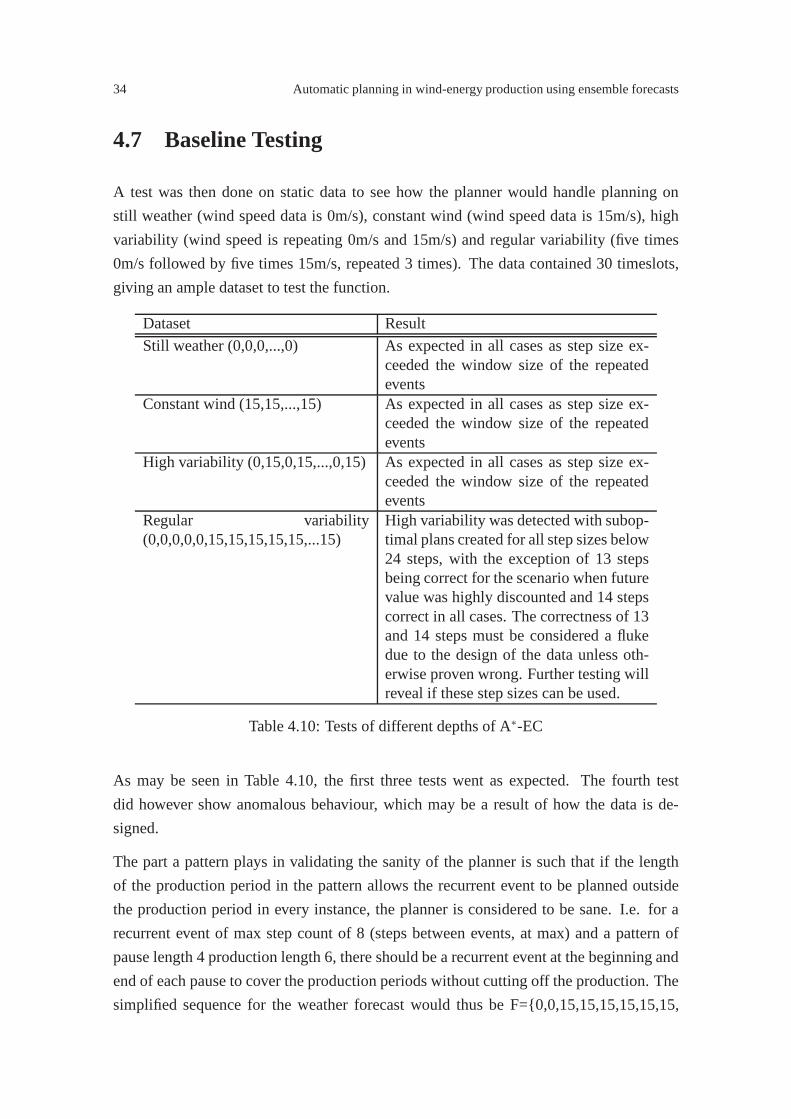
4.7 Baseline Testing
A test was then done on static data to see how the planner wouldhandle planning on
still weather (wind speed data is 0m/s), constant wind (windspeed data is 15m/s), high
variability (wind speed is repeating 0m/s and 15m/s) and regular variability (five times
0m/s followed by five times 15m/s, repeated 3 times). The datacontained 30 timeslots,
giving an ample dataset to test the function.
Dataset Result
Still weather (0,0,0,...,0) As expected in all cases as step size ex-ceeded the window size of the repeatedevents
Constant wind (15,15,...,15) As expected in all cases as step size ex-ceeded the window size of the repeatedevents
High variability (0,15,0,15,...,0,15) As expected in all cases as step size ex-ceeded the window size of the repeatedevents
Regular variability(0,0,0,0,0,15,15,15,15,15,...15)
High variability was detected with subop-timal plans created for all step sizes below24 steps, with the exception of 13 stepsbeing correct for the scenario when futurevalue was highly discounted and 14 stepscorrect in all cases. The correctness of 13and 14 steps must be considered a flukedue to the design of the data unless oth-erwise proven wrong. Further testing willreveal if these step sizes can be used.
Table 4.10: Tests of different depths of A∗-EC
As may be seen in Table 4.10, the first three tests went as expected. The fourth test
did however show anomalous behaviour, which may be a result of how the data is de-
signed.
The part a pattern plays in validating the sanity of the planner is such that if the length
of the production period in the pattern allows the recurrentevent to be planned outside
the production period in every instance, the planner is considered to be sane. I.e. for a
recurrent event of max step count of 8 (steps between events,at max) and a pattern of
pause length 4 production length 6, there should be a recurrent event at the beginning and
end of each pause to cover the production periods without cutting off the production. The
simplified sequence for the weather forecast would thus be F={0,0,15,15,15,15,15,15,

Þór Sigurðsson 35
0,0,0,0,15,15,15,15,15,15, 0,0,0,0,15,15,15,15,15,15,0,0} and the resulting plan should
be like P={ ID,MA,SU,P,P,P,P,P,SD,MA, ID,MA,SU,P,P,P,P,P,SD,MA, ID,MA,SU,P,P,P,P,P,SD,MA},
where ID=Idle, MA=Maintenance, SU=StartUp, P=Production, SD=ShutDown. 0 and 15
are meters per second wind strength.

36
37
Chapter 5
Results
In this chapter we present the results of the experiments performed. We start with the
simplest type of planner where we show that it does not perform adequately. We then
go through the different heuristics tested and show our findings for each one. At the end
of the chapter we present the findings of Yamaguchi and Ishihara (2008) and how they
correlate with our own findings. We planned against conventional weather forecasts and
ensemble forecasts to create plans. These plans were then used to simulate the production
using measured wind data. We then evaluated the bottom line of the power plant. We did
this for different periods and different heuristics. We present the results here.
5.1 Planning against a conventional weather forecast
The first version of the planner planned against a conventional weather forecast. The fore-
cast used was the baseline member of the ensemble forecast (called “gec00”). The data
stream is a timeline of single estimates of events (wind strength). The function used to
sense to these events is straight forward - if the wind strength is above a certain minimum,
production takes place. As may be seen in Figures 5.1a the planner does not succeed at in-
terpreting the weather well enough to justify planning beyond the first few hours, for this
specific case. In Figure 5.1b, we see the lack of correlation between the actual measured
weather (jagged green line) and the planned weather (stepwise blue line). The horizontal
red line signifies the breakout point where production ceases. The lack of correlation, as
seen in timesteps 40-55 and again in 145-165 may happen for a variety of reasons. The
landscape may affect the forecast (solved with a higher resolution weather forecast), or
the member may be interpreting the weather system incorrectly - e.g. unforeseen vertical
changes, temporal variations or spatial variations. Thesevariations are supposedly caught
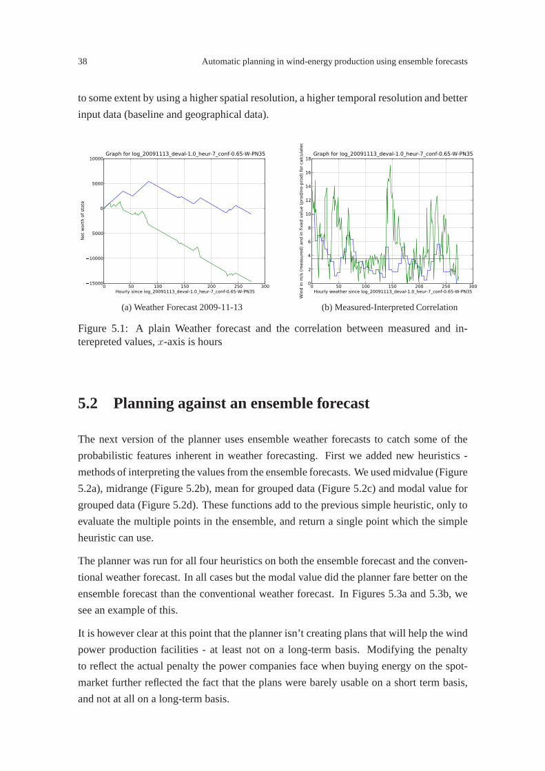
38 Automatic planning in wind-energy production using ensemble forecasts
to some extent by using a higher spatial resolution, a highertemporal resolution and better
input data (baseline and geographical data).
0 50 100 150 200 250 300Hourly since log_20091113_deval-1.0_heur-7_conf-0.65-W-PN35
�15000
�10000
�5000
0
5000
10000
Net
wort
h o
f st
ate
Graph for log_20091113_deval-1.0_heur-7_conf-0.65-W-PN35
(a) Weather Forecast 2009-11-13
0 50 100 150 200 250 300Hourly weather since log_20091113_deval-1.0_heur-7_conf-0.65-W-PN35
0
2
4
6
8
10
12
14
16
18
Win
d in m
/s (
measu
red)
and in f
ixed v
alu
e (
pro
d/n
o-p
rod)
for
calc
ula
ted
Graph for log_20091113_deval-1.0_heur-7_conf-0.65-W-PN35
(b) Measured-Interpreted Correlation
Figure 5.1: A plain Weather forecast and the correlation between measured and in-terepreted values,x-axis is hours
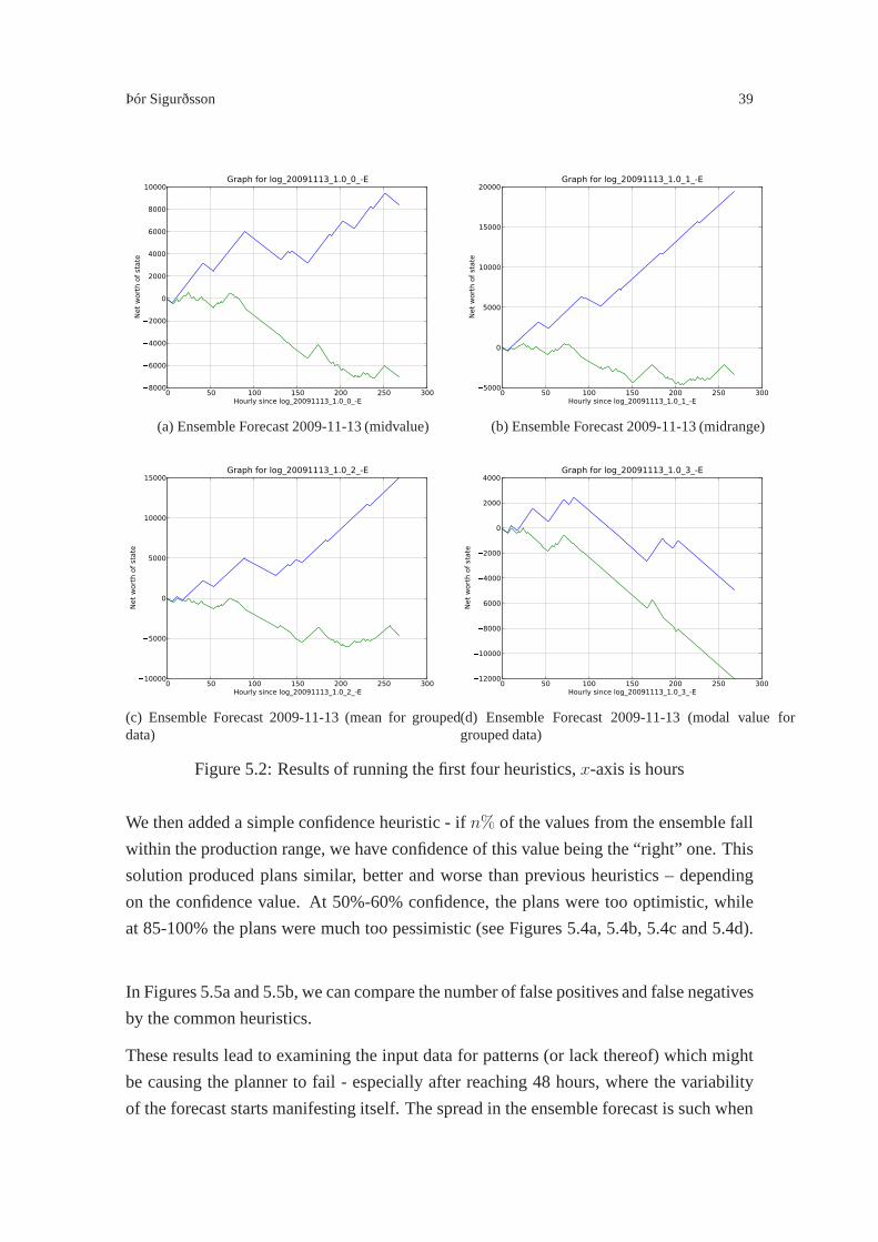
5.2 Planning against an ensemble forecast
The next version of the planner uses ensemble weather forecasts to catch some of the
probabilistic features inherent in weather forecasting. First we added new heuristics -
methods of interpreting the values from the ensemble forecasts. We used midvalue (Figure
5.2a), midrange (Figure 5.2b), mean for grouped data (Figure 5.2c) and modal value for
grouped data (Figure 5.2d). These functions add to the previous simple heuristic, only to
evaluate the multiple points in the ensemble, and return a single point which the simple
heuristic can use.
The planner was run for all four heuristics on both the ensemble forecast and the conven-
tional weather forecast. In all cases but the modal value didthe planner fare better on the
ensemble forecast than the conventional weather forecast.In Figures 5.3a and 5.3b, we
see an example of this.
It is however clear at this point that the planner isn’t creating plans that will help the wind
power production facilities - at least not on a long-term basis. Modifying the penalty
to reflect the actual penalty the power companies face when buying energy on the spot-
market further reflected the fact that the plans were barely usable on a short term basis,
and not at all on a long-term basis.
Þór Sigurðsson 39
0 50 100 150 200 250 300Hourly since log_20091113_1.0_0_-E
�8000
�6000
�4000
�2000
0
2000
4000
6000
8000
10000
Net
wort
h o
f st
ate
Graph for log_20091113_1.0_0_-E
(a) Ensemble Forecast 2009-11-13 (midvalue)
0 50 100 150 200 250 300Hourly since log_20091113_1.0_1_-E
�5000
0
5000
10000
15000
20000
Net
wort
h o
f st
ate
Graph for log_20091113_1.0_1_-E
(b) Ensemble Forecast 2009-11-13 (midrange)
0 50 100 150 200 250 300Hourly since log_20091113_1.0_2_-E
�10000
�5000
0
5000
10000
15000
Net
wort
h o
f st
ate
Graph for log_20091113_1.0_2_-E
(c) Ensemble Forecast 2009-11-13 (mean for groupeddata)
0 50 100 150 200 250 300Hourly since log_20091113_1.0_3_-E
�12000
�10000
�8000
�6000
�4000
�2000
0
2000
4000
Net
wort
h o
f st
ate
Graph for log_20091113_1.0_3_-E
(d) Ensemble Forecast 2009-11-13 (modal value forgrouped data)
Figure 5.2: Results of running the first four heuristics,x-axis is hours
We then added a simple confidence heuristic - ifn% of the values from the ensemble fall
within the production range, we have confidence of this valuebeing the “right” one. This
solution produced plans similar, better and worse than previous heuristics – depending
on the confidence value. At 50%-60% confidence, the plans weretoo optimistic, while
at 85-100% the plans were much too pessimistic (see Figures 5.4a, 5.4b, 5.4c and 5.4d).
In Figures 5.5a and 5.5b, we can compare the number of false positives and false negatives
by the common heuristics.
These results lead to examining the input data for patterns (or lack thereof) which might
be causing the planner to fail - especially after reaching 48hours, where the variability
of the forecast starts manifesting itself. The spread in theensemble forecast is such when
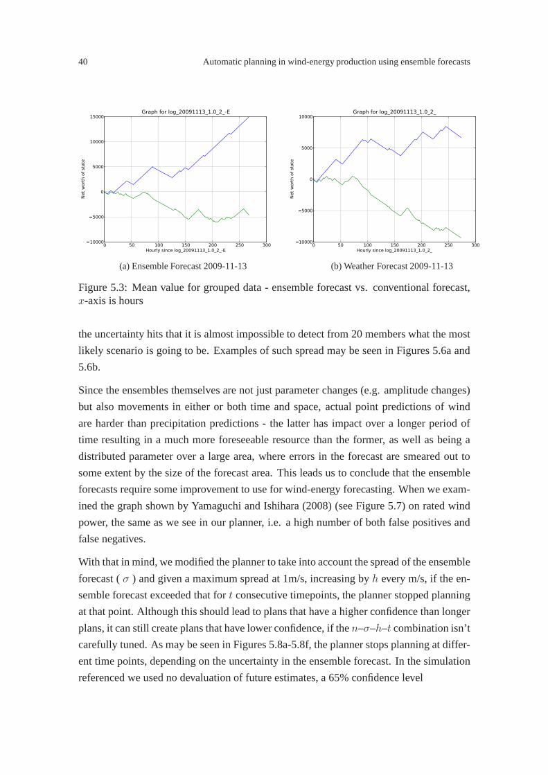
40 Automatic planning in wind-energy production using ensemble forecasts
0 50 100 150 200 250 300Hourly since log_20091113_1.0_2_-E
�10000
�5000
0
5000
10000
15000
Net
wort
h o
f st
ate
Graph for log_20091113_1.0_2_-E
(a) Ensemble Forecast 2009-11-13
0 50 100 150 200 250 300Hourly since log_20091113_1.0_2_
�10000
�5000
0
5000
10000
Net
wort
h o
f st
ate
Graph for log_20091113_1.0_2_
(b) Weather Forecast 2009-11-13
Figure 5.3: Mean value for grouped data - ensemble forecast vs. conventional forecast,x-axis is hours
the uncertainty hits that it is almost impossible to detect from 20 members what the most
likely scenario is going to be. Examples of such spread may beseen in Figures 5.6a and
5.6b.
Since the ensembles themselves are not just parameter changes (e.g. amplitude changes)
but also movements in either or both time and space, actual point predictions of wind
are harder than precipitation predictions - the latter has impact over a longer period of
time resulting in a much more foreseeable resource than the former, as well as being a
distributed parameter over a large area, where errors in theforecast are smeared out to
some extent by the size of the forecast area. This leads us to conclude that the ensemble
forecasts require some improvement to use for wind-energy forecasting. When we exam-
ined the graph shown by Yamaguchi and Ishihara (2008) (see Figure 5.7) on rated wind
power, the same as we see in our planner, i.e. a high number of both false positives and
false negatives.
With that in mind, we modified the planner to take into accountthe spread of the ensemble
forecast (σ ) and given a maximum spread at 1m/s, increasing byh every m/s, if the en-
semble forecast exceeded that fort consecutive timepoints, the planner stopped planning
at that point. Although this should lead to plans that have a higher confidence than longer
plans, it can still create plans that have lower confidence, if then–σ–h–t combination isn’t
carefully tuned. As may be seen in Figures 5.8a-5.8f, the planner stops planning at differ-
ent time points, depending on the uncertainty in the ensemble forecast. In the simulation
referenced we used no devaluation of future estimates, a 65%confidence level
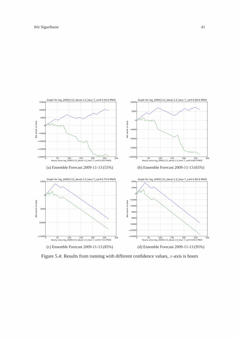
Þór Sigurðsson 41
0 50 100 150 200 250 300Hourly since log_20091113_deval-1.0_heur-7_conf-0.50-E-PN35
�20000
�15000
�10000
�5000
0
5000
10000
15000
Net
wort
h o
f st
ate
Graph for log_20091113_deval-1.0_heur-7_conf-0.50-E-PN35
(a) Ensemble Forecast 2009-11-13 (55%)
0 50 100 150 200 250 300Hourly since log_20091113_deval-1.0_heur-7_conf-0.60-E-PN35
�20000
�15000
�10000
�5000
0
5000
10000
Net
wort
h o
f st
ate
Graph for log_20091113_deval-1.0_heur-7_conf-0.60-E-PN35
(b) Ensemble Forecast 2009-11-13 (65%)
0 50 100 150 200 250 300Hourly since log_20091113_deval-1.0_heur-7_conf-0.75-E-PN35
15000
10000
5000
0
5000
Net
wort
h o
f st
ate
Graph for log_20091113_deval-1.0_heur-7_conf-0.75-E-PN35
(c) Ensemble Forecast 2009-11-13 (85%)
0 50 100 150 200 250 300Hourly since log_20091113_deval-1.0_heur-7_conf-0.85-E-PN35
14000
12000
10000
8000
6000
4000
2000
0
2000
4000
Net
wort
h o
f st
ate
Graph for log_20091113_deval-1.0_heur-7_conf-0.85-E-PN35
(d) Ensemble Forecast 2009-11-13 (95%)
Figure 5.4: Results from running with different confidence values,x-axis is hours
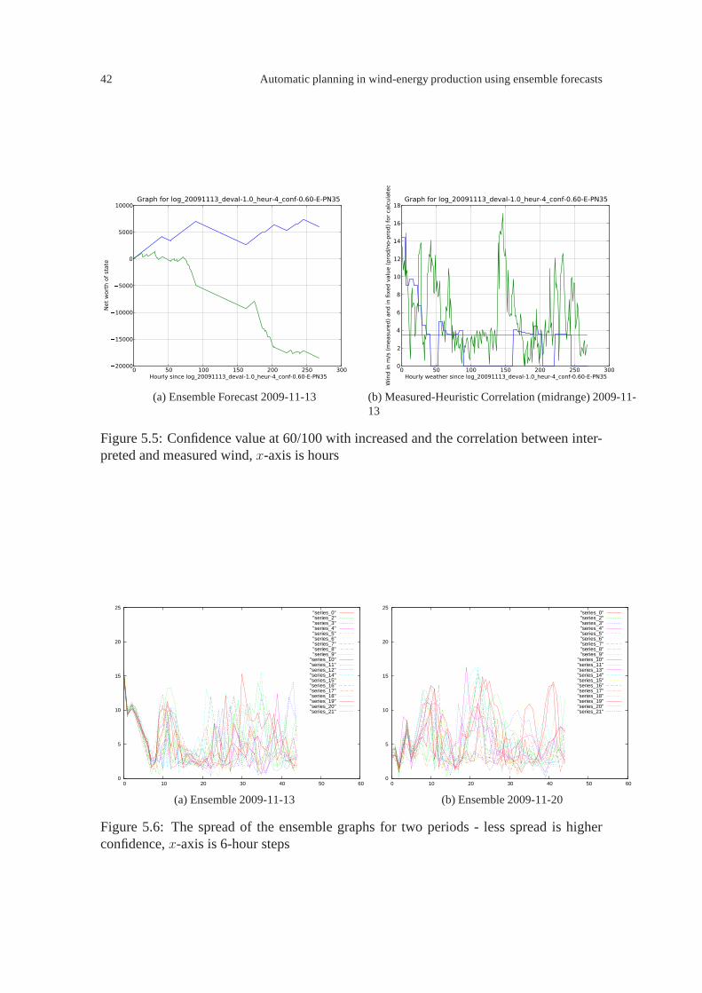
42 Automatic planning in wind-energy production using ensemble forecasts
0 50 100 150 200 250 300Hourly since log_20091113_deval-1.0_heur-4_conf-0.60-E-PN35
�20000
�15000
�10000
�5000
0
5000
10000
Net
wort
h o
f st
ate
Graph for log_20091113_deval-1.0_heur-4_conf-0.60-E-PN35
(a) Ensemble Forecast 2009-11-13
0 50 100 150 200 250 300Hourly weather since log_20091113_deval-1.0_heur-4_conf-0.60-E-PN35
0
2
4
6
8
10
12
14
16
18
Win
d in m
/s (
measu
red)
and in f
ixed v
alu
e (
pro
d/n
o-p
rod)
for
calc
ula
ted
Graph for log_20091113_deval-1.0_heur-4_conf-0.60-E-PN35
(b) Measured-Heuristic Correlation (midrange) 2009-11-13
Figure 5.5: Confidence value at 60/100 with increased and thecorrelation between inter-preted and measured wind,x-axis is hours
0
5
10
15
20
25
0 10 20 30 40 50 60
"series_0""series_2""series_3""series_4""series_5""series_6""series_7""series_8""series_9"
"series_10""series_11""series_12""series_14""series_15""series_16""series_17""series_18""series_19""series_20""series_21"
(a) Ensemble 2009-11-13
0
5
10
15
20
25
0 10 20 30 40 50 60
"series_0""series_2""series_3""series_4""series_5""series_6""series_7""series_8""series_9"
"series_10""series_11""series_13""series_14""series_15""series_16""series_17""series_18""series_19""series_20""series_21"
(b) Ensemble 2009-11-20
Figure 5.6: The spread of the ensemble graphs for two periods- less spread is higherconfidence,x-axis is 6-hour steps
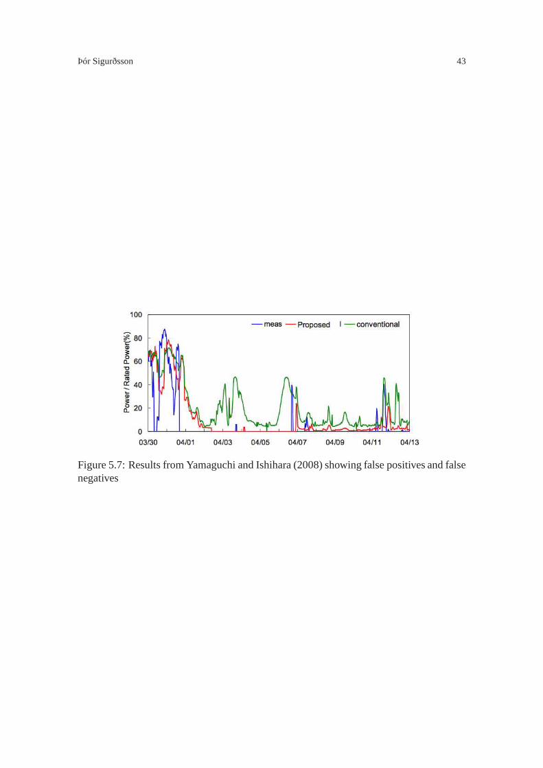
Þór Sigurðsson 43
Figure 5.7: Results from Yamaguchi and Ishihara (2008) showing false positives and falsenegatives
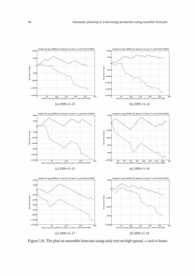
44 Automatic planning in wind-energy production using ensemble forecasts
0 50 100 150 200 250 300Hourly since log_20091113_deval-1.0_heur-7_conf-0.65-E-PN35
�20000
�15000
�10000
�5000
0
5000
10000
Net
wort
h o
f st
ate
Graph for log_20091113_deval-1.0_heur-7_conf-0.65-E-PN35
(a) 2009-11-13
0 50 100 150 200 250 300Hourly since log_20091114_deval-1.0_heur-7_conf-0.65-E-PN35
25000
20000
15000
10000
5000
0
5000
10000
Net
wort
h o
f st
ate
Graph for log_20091114_deval-1.0_heur-7_conf-0.65-E-PN35
(b) 2009-11-14
0 50 100 150 200Hourly since log_20091115_deval-1.0_heur-7_conf-0.65-E-PN35
�12000
�10000
�8000
�6000
�4000
�2000
0
2000
4000
Net
wort
h o
f st
ate
Graph for log_20091115_deval-1.0_heur-7_conf-0.65-E-PN35
(c) 2009-11-15
0 20 40 60 80 100 120 140 160 180Hourly since log_20091116_deval-1.0_heur-7_conf-0.65-E-PN35
�10000
�8000
�6000
�4000
�2000
0
2000
Net
wort
h o
f st
ate
Graph for log_20091116_deval-1.0_heur-7_conf-0.65-E-PN35
(d) 2009-11-16
0 50 100 150 200Hourly since log_20091117_deval-1.0_heur-7_conf-0.65-E-PN35
�14000
�12000
�10000
�8000
�6000
�4000
�2000
0
2000
4000
Net
wort
h o
f st
ate
Graph for log_20091117_deval-1.0_heur-7_conf-0.65-E-PN35
(e) 2009-11-17
0 50 100 150 200 250 300Hourly since log_20091118_deval-1.0_heur-7_conf-0.65-E-PN35
�20000
�15000
�10000
�5000
0
5000
Net
wort
h o
f st
ate
Graph for log_20091118_deval-1.0_heur-7_conf-0.65-E-PN35
(f) 2009-11-18
Figure 5.8: The plan on ensemble forecasts using early exit on high spread,x-axis is hours
45
Chapter 6
Conclusions
In the power production sector, automatic planning is a feasible tool. It gives us the
opportunity to try out a variety of solutions in much greaternumbers than manual planning
allows us. It can also suggest a number of “best solutions” based on search criteria, and
it will avoid mistakes which can happen in manual planning where a bad plan may be
elevated above the good plans.
Once we have the rulesets for how the model is supposed to behave, we can set our
heuristics (see Tables 4.3, 4.4, and Equation 4.7)
We addressed the heuristics problem and ran the model on the conventional weather fore-
cast and showed that such runs in general don’t work beyond 0-3 days, depending on
how far into the future the conventional weather forecast actually manages to keep its
accuracy - accuracy that is solely based on a single timelineof events. This is a real
problem for planning, since planning usually works by evaluating the likelihood of an
event taking place, and selecting the best action (according to a heuristic) in light of the
probabilities.
We then did the same for ensemble forecasts, using a variety of heuristics to evaluate the
distribution between members. We did get better results, and we also got a few ideas
worth exploring further in terms of planning techniques.
The weather forecasts were, as mentioned before, fairly accurate for a period of up to 3
days. In that period, plans were somewhat correct (or at least more correct than not). The
problem however persists that the quality of the plans must stay at a relatively high level
for them to be valuable tools to use in planning for power production. Planning against
conventional weather forecasts does not solve that issue.

46 Automatic planning in wind-energy production using ensemble forecasts
This leads us to the ensemble forecasts and how they perform.They don’t fix the problem,
but they do perform a little better. Also, by using the confidence value, the planner may be
terminated or programmed to "ignore" periods of high uncertainty, since such uncertainty
has little value in planning. This uncertainty is clearly visible just by plotting the data sets
(see Figures 5.6a and 5.6b). As can be seen on the figures, whenthe members get close
to one another, the confidence level rises, and when they spread out, the confidence level
decreases.
One of the problems we face is the inaccuracy of the ensemble forecasts. With a high
spread on the members, we have a low confidence on what is goingto happen. This can be
fixed somewhat by improving the models with high-resolutionspatial data (GalileoCast:
Foreca Consulting Main Page, 2011) and point-in-time weather data using UAVs (Vilhjálmsson,
2010).Reiknistofa í Veðurfræði(2011) has been working on both of these projects as well
as on a method of incorporating high-resolution ASTER data (ASTER: Advanced Space-
borne Thermal Emission and Reflection Radiometer(2011)) into WRF, gaining increased
accuracy for high-resolution (temporal and spatial) weather forecasts, e.g. for the island of
Utsira in Norway. At Gufuskálar, there has been work underway to collect high-resolution
weather data at several levels (10m, 40m, 100m, 200m, 400m) to be able to profile certain
weather events in greater detail than possible before.
The planner can use the information in the ensemble forecasts to gain the advantage of
many partial plans for the period in question, using the confidence level of the members
to select whether to plan or to ignore. These partial plans may then be combined with
previously made plans for the same period to create a better plan-set for a longer period.
What we do is to make plans for times that are “known” to be stable, and attempt to
fill in the blanks with older information or search based plans. Even just-in-time (JIT)
planning if that’s what we want. Since the wind is the most difficult element of the
weather forecasts, we can be sure that since it does work fairly well for shorter periods
of time with the rather vague input data available, it will work much better for systems
that have even greater stability and slower rate of change than wind, e.g. hydropower and
geothermal power (groundwater, rain, melt).

47
Bibliography
Aster: Advanced spaceborne thermal emission and reflectionradiometer. (2011, 04).
Retrieved 2011-04-28, fromhttp://asterweb.jpl.nasa.gov/
Bluman, A. G. (2008).Elementary statistics - a step by step approach(M. HILL, Ed.).
McGRAW HILL.
Bresina, J. L., Jónsson, A. K., Morris, P. H., & Rajan, K. (2005). Activity Planning
for the Mars Exploration Rovers. In15th International Conference on Automated
Planning and Scheduling (ICAPS).
Europa pso platform for ai planning, scheduling, constraint program-
ming and optimization. (2011, 04). Retrieved 2011-04-28, from
http://code.google.com/p/europa-pso/
Evolution of ecmwf forecast skill for varying lead times. (2011, 05). Re-
trieved 2011-05-14, from http://www.nap.edu/books/12878/
xhtml/images/p2001b959g23001.jpg
Galileocast: Foreca consulting main page.(2011, 04). Retrieved 2011-04-28, from
http://www.forecaconsulting.com/galileocast/
Garrad-hassan webpage. (2011, 03). Retrieved 2011-03-07, from
http://www.gl-garradhassan.com/en/index.php
Grell, G. A., Dudhia, J., & Stauffer, D. R. (1995).A Description of the Fifth–Generation
Penn State/NCAR Mesoscale Model (MM5). NCAR/TN–398+STR.National Center
for Atmospheric Research, Boulder, CO, 107 pp.
Img: Cloud. (2011, 2). Retrieved 2011-02-26 via images.google.com, from
http://www.usatoday.com
Img: Cluster. (2011, 02). Retrieved 2011-02-26 via images.google.com, from
http://tik.ee.ethz.ch
Img: House.(2011, 02). Retrieved 2011-02-26, fromhttp://etc.usf.edu
Img: Windmill. (2011, 02). Retrieved 2011-02-26, from
http://jonathanhaynes.com
48 Automatic planning in wind-energy production using ensemble forecasts
Jónsson, A. K., McGann, C., Pedersen, L., Iatauro, M., & Rajagopalan, S. (2005, Septem-
ber). Autonomy Software Architecture for LORAX (Life On IceRobotic Antartic
Explorer). InInt’l Symposium on Artificial Intelligence, Robotics and Automation
in Space (iSAIRAS).Münich, Germany.
Kim, J. H., & Han, C. (2001, March). Short-Term Multiperiod Optimal Planning of
Utility Systems Using Heuristics and Dynamic Programming.Industrial & Engi-
neering Chemistry Research, 40(8), 1928-1938.
Kjeldsen, A. (n.d.). Tvindmøllen.jpg. Available
from http://upload.wikimedia.org/wikipedia/
commons/7/77/Tvindmøllen.jpg
Landsnet spot-market prices. (2011, 5). Retrieved 2011-05-11, from
http://landsnet.is/raforkukerfid/jofnunarorka/
jofnunarorkuverd/index.aspx?GroupId=791
Matplotlib webpage. (2011, 03). Retrieved 2011-03-07, from
http://matplotlib.sourceforge.net/
Mm5 website. (2010, 9). WebPage. Available from
http://www.mmm.ucar.edu/mm5
Nielsen, H. A., Nielsen, T. S., Madsen, H., Giebel, G., Badger, J., Landberg, L., et al.
(2006). From wind ensembles to probabilistic information about future wind power
production - results from an actual application. In9th international conference
on probabilistic methods applied to power systems, kth, stockholm, sweden - june
11-15, 2006.
Noaa gfs webpage. (2011, 03). Retrieved 2011-03-05, from
http://www.emc.ncep.noaa.gov/gmb/ens/
Reiknistofa í veðurfræði. (2011, 02). Retrieved 2011-02-26, from
http://www.riv.is
Russell, S., & Norvig, P. (2003).Artificial intelligence, a modern approach. Prentice
Hall.
Sigurðsson Þór, Jónsson, D. A. K., & Rögnvaldsson, Ó. (2009). Climate and utility
operations(Tech Report - Research Project). Reykjavik University andInstitute for
Meteorological Research.
Skamarock, W. C., Klemp, J. B., Dudhia, J., Gill, D. O., Barker, D. M., Duda, M. G., et al.
(2008). A Description of the Advanced Research WRF Version 3. NCAR Technical
Note, NCAR/TN–475+(STR).National Center for Atmospheric Research, Boulder,
CO, 113 pp.
Vilhjálmsson, S. E. (2010).Fjarskiptavæðing mannlausra flugvéla.

Þór Sigurðsson 49
Wikimedia: Picture of weather model. (2011, 05). Retrieved 2011-
05-14, from http://upload.wikimedia.org/wikipedia/
commons/7/73/AtmosphericModelSchematic.png
Wrf website. (2010, 9). WebPage. Available from
http://www.wrf-model.org/index.php
Yamaguchi, A., & Ishihara, T. (2008).Wind Power Forecast based on ARX Model
with Multi Time Scale Parameter. Unpublished master’s thesis, The University of
Tokyo.
Zachmann, G. (n.d.). Convergence of wholesale elec-
tricity spot prices in europe? Available from
http://www.sessa.eu.com/documents/18_Zachmann.pdf
Zhang, H., & Pu, Z. (2010). Beating the uncertainties: Ensemble forecasting and
ensemble-based data assimilation in modern numerical weather prediction. Ad-
vances in Meteorology, 2010, 10.

50

51
Appendix A
Appendix
A.1 The Planner
A.1.1 The planner options
>java -jar mscPlanner.jar -?
System options:
-? : This help
-h : This help
-v : Verbose (false)
-y n : Year, 0<n<now (2009)
-m n : Month, 1<=n<=12 (12)
-d n : Day, 1<=n<=(max day of month) (28)
-H n: The heuristic to use for planning, 0<=n<=5 (0)
0: Midvalue
1: Midrange
2: Mean for grouped data
3: Modal class for grouped data
4: Confidence levels
5: BASELINE
6: gec00 best fit
7: Confidence levels using stddev
-MD n: The maximum number of datapoints to consider, regardl ess of the length of the series
-cl n: The confidence level of the data
-cr n: The confidence range of the data
-B n : Break (early commit) if OpenList contains at least n nod es
-smd n: The maximum deviation allowed at 1.0m/s
-ssl n: The slant of the maximum deviation
-sms n: The maximum number of successive ’bad’ days
-hD n: The constant to devalue the future heuristic by (defau lt: 1.0, less than 1.0 is devalue)
-ss n: The number of steps to start with (5)
-es n: The number of steps to end with (9)
-E : Use ensemble forecast
-W : Use weather forecast (default)
-eB n: The ensemble breakpoint (default: 0.7)
-f fn: The filename to use for plant definitions (default: De faultFactories.yml)
-c fn: The filename of the system configuration file (defaul t: plannerConfig.yml)
-lf fn: The filename of the logfile to use (default: none)
-L fn: The filename of the debug logfile to use (default: none )
-ll n: The loglevel to use (from 0 through 7, default: 4)
-svx n: the carry of service days between planning sessions w here 0<=x<=4
-RD : Only read the data from the database, and then quit.
-PP n: Production cost when production is planned
-PN n: Production cost when prodiction is planned but fails
-NN n: Production cost when production is not planned
-SC n: Service cost
-wdm n: Weather data multiplier for measured data (warning: will skew results! - default 1.0)

52 Automatic planning in wind-energy production using ensemble forecasts
-SD : Simulate measured data by usung calculated data instea d
-bp n: Backpedal n levels at fork (default is 1)
>
The options available to the user in the planning program


School of Computer ScienceReykjavík UniversityMenntavegi 1101 Reykjavík, IcelandTel. +354 599 6200Fax +354 599 6201www.reykjavikuniversity.isISSN 1670-8539