Automatic Temperature Setpoint Tuning of a

Thermoforming Machine using Fuzzy Terminal

Iterative Learning Control

Mathieu Beauchemin-Turcotte∗, Guy Gauthier∗†

and Robert Sabourin∗

April 5, 2019

Abstract

This paper presents a new way to design a Fuzzy Terminal Iterative LearningControl (TILC) to control the heater temperature setpoints of a thermoform-ing machine. This fuzzy TILC is based on the inverse of a fuzzy model of thismachine, and is built from experimental (or simulation) data with kriging in-terpolation. The Fuzzy Inference System usually used for a fuzzy model is thezero order Takagi Sugeno Kwan system (constant consequents). In this paper,the 1st order Takagi Sugeno Kwan system is used, with the fuzzy model rulesexpressed using matrices. This makes the inversion of the fuzzy model mucheasier than the inversion of the fuzzy model based on the TSK of order 0. Basedon simulation results, the proposed fuzzy TILC seems able to give a very goodinitial guess as to the heater temperature setpoints, making it possible to havealmost no wastage of plastic sheets. Simulation results show the effectiveness ofthe fuzzy TILC compared to a crisp TILC, even though the fuzzy controller isbased on a fuzzy model built from noisy data.

Keywords

Fuzzy internal model control, fuzzy modeling, kriging interpolation, terminaliterative learning control.

∗Affiliated with Department of automated engineering, Ecole de technologie superieure,Montreal, Canada.†Corresponding author: guy.gauthier@etsmtl.ca

1

arX

iv:1

703.

0978

9v1

[cs

.SY

] 2

8 M

ar 2

017

1 Introduction

The thermoforming process plays an important role in the plastics industry. InNorth America in 2003, in excess of $10 billion worth of thermoformed partswere produced [1]. Examples of the parts fabricated using this process includecar bumpers, baths, and packaging products, among numerous others.

The plastic sheets used in the thermoforming process undergo three phases[2, 3, 4]. The reheat phase, where the plastic sheet is heated to a sufficientlyhigh temperature to render it malleable; the molding phase; and the coolingphase. The malleable plastic sheet is draped over a mold to give it the desiredshape, and then cooled in the mold until it becomes rigid again. Finally, in thetrimming phase, excess plastic is removed to obtain a usable part.

In this paper, we address only issues arising in the reheat phase of thethermoforming process. This phase is critical, since the molding will not beaccurate if the plastic sheet is not heated correctly [3, 5], resulting in rejectionof the inaccurately molded part by the quality control department.

To heat the plastic sheet correctly, the heater temperature setpoints haveto be appropriately adjusted. This adjustment is performed by the operator ofthe machine using a trial-and-error approach. This approach results in plasticsheets being wasted, and occurs mostly at the start of a new production lot.It also occurs when the temperature in the plant changes significantly afterthe adjustment is made. In North America, plastic sheet wastage during themanufacture of a component can represent up to 10 to 15% of each productionlot. For complicated parts, this percentage can rise to 20% [3].

An experienced operator can successfully reduce these losses. However, plas-tics processing companies are struggling to find qualified and experienced peopleto operate their thermoforming machines. Their fear now is that a large numberof these employees will reach retirement age over the next few years.

Very little work has been published regarding the control of sheet surfacetemperature [6]. Such a control system would improve the quality of the partsproduced, reduce scrap, and allow for temperature zoning. Plastic sheet tem-perature is controlled by adjusting the heater temperature of the thermoformingmachine, and this control must be such that the plastic sheet temperature con-verges to a desired temperature profile. This issue belongs to a class of problemsknown as ”inverse heating problems” (IHP) [7].

Existing TILC algorithms are highly dependent on initial guesswork withregard to temperature setpoints. When the initial guess is near the temperaturesetpoint required to heat a plastic sheet correctly, all is well. But, when it is not,a number of cycles are required to converge to the right value, causing wastageof plastic sheets. By increasing the controller gain, the convergence speed canbe improved, but at the cost of less robustness. Furthermore, with those highgains, the system can be subject to overshoot. For a thermoforming oven, this isa serious problem, since there is a risk that a very malleable, overheated plasticsheet will fall on the bottom heaters, forcing the process to be stopped in orderto clean them.

A suitable approach that makes this initial guess reliably would be a major

2

improvement in the control of this kind of process, where money needs to besaved by reducing wastage. It would result in the right heater temperaturesetpoints being determined at the start of the process, and reduce the controllergain perturbations, improving robustness.

The selected control approach is a TILC based on an inverse fuzzy model.This nonlinear control approach permits a relatively good initial guess of heatertemperature setpoints from a desired surface temperature profile of the plasticsheet. The design approach presented here provides the opportunity to use datafrom a reliable nonlinear model, or from the process itself. This fuzzy approachhas never been used for a TILC. The main contribution of this paper is the useof the 1st order Takagi Sugeno Kwan Fuzzy Inference System, along with itsrule consequent, expressed in matrix form and built from kriging interpolation.

In this paper, we make a number of assumptions: 1) That the ambienttemperature is constant (this assumption is relaxed in the simulations results);2) That the initial temperature of the plastic sheet is constant; 3) That theplastic sheet is homogeneous and not subject to sag; 4) That the PID loops, inwhich the setpoints interact with the heater [4], have reached their steady statewhen the plastic sheet is heated; 5) That the number of inputs is equal to thenumber of outputs; and 6) That the minimal and maximal output values arelocated at opposite corners of the input space. This last assumption fits wellwith the way the thermoforming oven functions, since the plastic sheet surfacetemperature is minimal when all the heaters are at minimal temperature, andmaximal when all the heaters are at maximal temperature.

The paper is structured as follows. Related works are covered in section2. A system overview is provided in section 3. Section 4 explains how thefuzzy model of a nonlinear process is obtained. Section 5 shows the steps tofollow to invert the fuzzy model, giving the inverse fuzzy model componentof the TILC (Figure 3). Section 6 concerns the fuzzy filter used in the fuzzyTILC that adjusts the heater temperature setpoints of the thermoforming oven.Section 7 presents the case of a fuzzy TILC applied to a six heater, six sensorthermoforming oven model, and simulation results demonstrate how the fuzzyTILC behaves. Finally, we provide our conclusions in section 8.

2 Related works

2.1 Introducing Terminal Iterative Learning Control

Analysis of this temperature control problem gave us the idea of using a cycle-to-cycle approach to automatically tune the heater temperature setpoints, and ledto considering a Terminal Iterative Learning Control (TILC). This approach wasfirst introduced in [8] and then in a Ph.D. thesis [9], and is derived from IterativeLearning Control (ILC) [9, 10]. It has been used for the cycle-to-cycle control of aRapid Thermal Process and Chemical Vapor Deposition (RPTCVD) [8, 9, 11].The main difference between ILC and TILC is that ILC uses measurementssampled along the entire cycle, while TILC only uses measurements sampled at

3

Figure 1: Block diagram of a TILC controlled system

the end of the cycle.The TILC is based on certain assumptions [9, 10, 12]:

• That the cycle length T ∈ R has a fixed duration;

• That the input vector u[k] ∈ Rm is maintained constant during the entirecycle k (k ∈ N);

• That the process parameters can vary in the time domain (t) but areinvariant in the cycle domain (k);

• That the process start always with the same initial state vector x0 ∈ Rn,so x0[k] = x0 ∀k;

• That the desired output vector yd ∈ Rp must be feasible, so an inputvector u[k] ∈ Rm must exist that made the terminal output yT [k] ∈ Rp

equal to yd; and, finally,

• That this input vector u[k] must be unique.

These assumptions fit relatively well with the thermoforming reheat phase.To use the TILC approach on a thermoforming machine, temperature sensorsare installed to measure the surface temperature of the plastic sheet at the endof the heating cycle [4, 6, 12]. TILC iteratively adjusts the heater temperaturesetpoints, so that the sheet surface temperature converges to the desired levelat the end of the heating cycle [12].

The block diagram of a TILC algorithm is shown in Figure 1. The inputvector u[k], applied to the process during the entire cycle k, is a function ofthe terminal output vector yT [k− 1] measured at the end of the previous cycle(k−1), the corresponding input vector u[k−1] and the desired terminal outputvector yd. The simplest TILC algorithm (called a 1st order TILC) is expressedas follows:

u[k] = u[k − 1] + K(yd − yT [k − 1]) (1)

where K ∈ Rm×p is the matrix containing the TILC gains.

2.2 Other related control approaches

This problem has been addressed in semiconductor industry processes like theRapid Thermal Process and Chemical Vapor Deposition (RPTCVD), by theuse of run-to-run (R2R) control. Like TILC, the R2R algorithm uses only

4

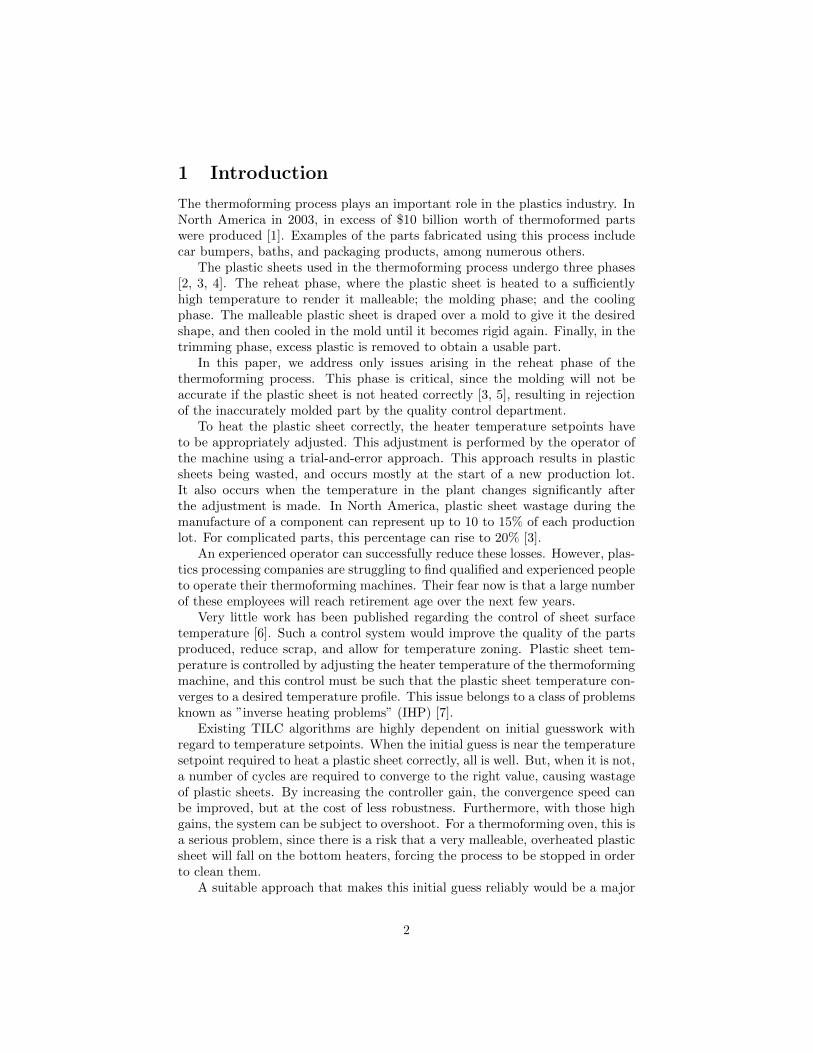
Figure 2: Internal model control structure (non-fuzzy)

measurements performed at the end of the cycle or later [13, 14, 15, 16]. TheR2R approach is composed of various control algorithms [14], the one most oftenused being the Exponential Weighting Moving Average (EWMA) [13, 14]. R2Rcontrol is an approach derived from statistical process control.

Papers [7, 17] cover control of the temperature profile of a plastic materialin roll-fed thermoforming. This control approach is based on a computationalfinite element algorithm, which is mainly based on the geometric relationshipbetween the heating elements and the plastic material. These relationships areused to compute the heater temperature setpoints. In [7], this inverse problemis considered to be an ill-posed problem, since two sets of heater temperaturesetpoints can give relatively similar surface temperature profiles. In [17], thesensitivity of the algorithm proposed in [7] to perturbations is studied.

In a recent paper [18], the plastic sheet temperature is controlled with atwo-dimensional fast Fourier transform (FFT) of the sheet temperature profile.This approach is also explained in a book chapter [19]. These authors have alsoproposed an alternative approach, based on the conjugate gradient method [5].

3 System overview

The fuzzy TILC (f-TILC) proposed in this paper is based on a TILC usinga fuzzy nonlinear internal model control (FNIMC). The non fuzzy TILC withInternal Model Control (IMC) proposed in the chapter 3 of [12] has the structureshown in Figure 2 (where GP is the process, GM is the process model, GC isthe controller and Q is the filter).

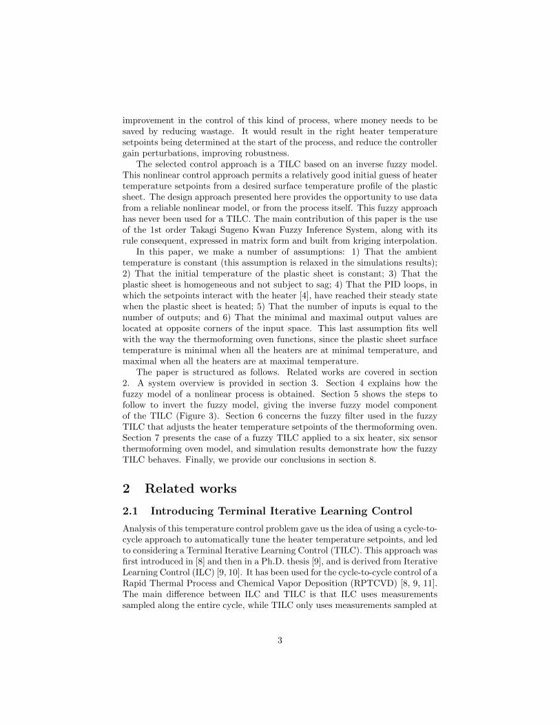
The block diagram of the proposed fuzzy TILC with IMC is shown in Figure3. This block diagram looks similar to the FNIMC block diagram shown inFigure 3 of [20], except for the z−1 block in the feedback.

In the block diagram of the proposed fuzzy TILC with IMC, the filter is alsoa fuzzy function that permits the TILC to exhibit a behavior, such that theconvergence of the output vector yT [k] to yd is relatively monotonic. It is usedto evaluate the corrected setpoint for the next cycle sp[k], which in turn is used

5

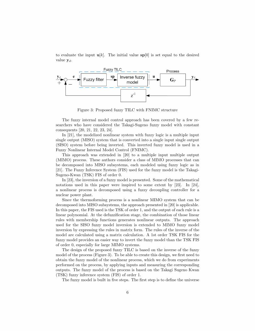
to evaluate the input u[k]. The initial value sp[0] is set equal to the desiredvalue yd.

Figure 3: Proposed fuzzy TILC with FNIMC structure

The fuzzy internal model control approach has been covered by a few re-searchers who have considered the Takagi-Sugeno fuzzy model with constantconsequents [20, 21, 22, 23, 24].

In [21], the modelized nonlinear system with fuzzy logic is a multiple inputsingle output (MISO) system that is converted into a single input single output(SISO) system before being inverted. This inverted fuzzy model is used in aFuzzy Nonlinear Internal Model Control (FNIMC).

This approach was extended in [20] to a multiple input multiple output(MIMO) process. These authors consider a class of MIMO processes that canbe decomposed into MISO subsystems, each modeled using fuzzy logic as in[21]. The Fuzzy Inference System (FIS) used for the fuzzy model is the Takagi-Sugeno-Kwan (TSK) FIS of order 0.

In [23], the inversion of a fuzzy model is presented. Some of the mathematicalnotations used in this paper were inspired to some extent by [23]. In [24],a nonlinear process is decomposed using a fuzzy decoupling controller for anuclear power plant.

Since the thermoforming process is a nonlinear MIMO system that can bedecomposed into MISO subsystems, the approach presented in [20] is applicable.In this paper, the FIS used is the TSK of order 1, and the output of each rule is alinear polynomial. At the defuzzification stage, the combination of those linearrules with membership functions generates nonlinear outputs. The approachused for the SISO fuzzy model inversion is extended to MIMO fuzzy modelinversion by expressing the rules in matrix form. The rules of the inverse of themodel are calculated using a matrix calculation. A 1st order TSK FIS for thefuzzy model provides an easier way to invert the fuzzy model than the TSK FISof order 0, especially for large MIMO systems.

The design of the proposed fuzzy TILC is based on the inverse of the fuzzymodel of the process (Figure 3). To be able to create this design, we first need toobtain the fuzzy model of the nonlinear process, which we do from experimentsperformed on the process, by applying inputs and measuring the correspondingoutputs. The fuzzy model of the process is based on the Takagi Sugeno Kwan(TSK) fuzzy inference system (FIS) of order 1.

The fuzzy model is built in five steps. The first step is to define the universe

6

of discourse of each input to the process, which corresponds to the variationbetween the minimum and maximum value of each input. The second step isto divide each defined universe of discourse into a number of fuzzy sets. Thethird step is to define the input vectors (also called input tuples) that need to beapplied to the process at the experimental stage, in order to obtain the rules ofthe fuzzy model. In the fourth step, which is the experimental stage, a databaseis built from the input vectors applied to the process and the correspondingoutput vectors measured in the experiments. The last step is to evaluate therules of the fuzzy model from the database of input and output vectors. This isdone using an approach not used in fuzzy control: kriging interpolation.

4 The fuzzy modeling of nonlinear processes

The following subsections explain each of the five steps listed above. The nota-tion used in this paper is introduced in each subsection.

4.1 Defining the universe of discourse of each input

From the knowledge available about the nonlinear process, the universe of dis-course of each input is defined to make it possible to build a fuzzy model of theprocess. The minimal value of the j-th input uj ∈ R is defined by umin,j andits maximal value by umax,j . Then, the universe of discourse of the j-th inputis uj ∈ Uj = [umin,j , umax,j ] ⊂ R.

The orthogonal combination of all the universes of discourses of the m inputsleads to an m dimension input space:

U = U1 × . . .× Um ∈ Rm (2)

so the input vector u = [u1, . . . , um]T ∈ U.The universes of discourse are divided into a number of fuzzy sets.

4.2 Dividing the universe of discourse of each input intofuzzy sets

The universe of each input is covered by a certain number of fuzzy sets (Figure4), each of which is identified by a linguistic term. The i-th fuzzy set of the j-thinput is identified by the linguistic term Ai,j . The number of fuzzy sets definedfor the j-th input is identified by Nj ∈ N. The number of fuzzy sets has aneffect on the accuracy of the fuzzy model.

For the proposed fuzzy model, the membership functions of each fuzzy set aretriangular (see Figure 4). When i ∈ {2, . . . , Nj − 1}, the membership functionsare defined as follows:

µAi,j(uj) =

n1/m1 ai−1,j ≤ uj ≤ ai,jn2/m2 ai,j < uj ≤ ai+1,j

0 otherwise

(3)

7

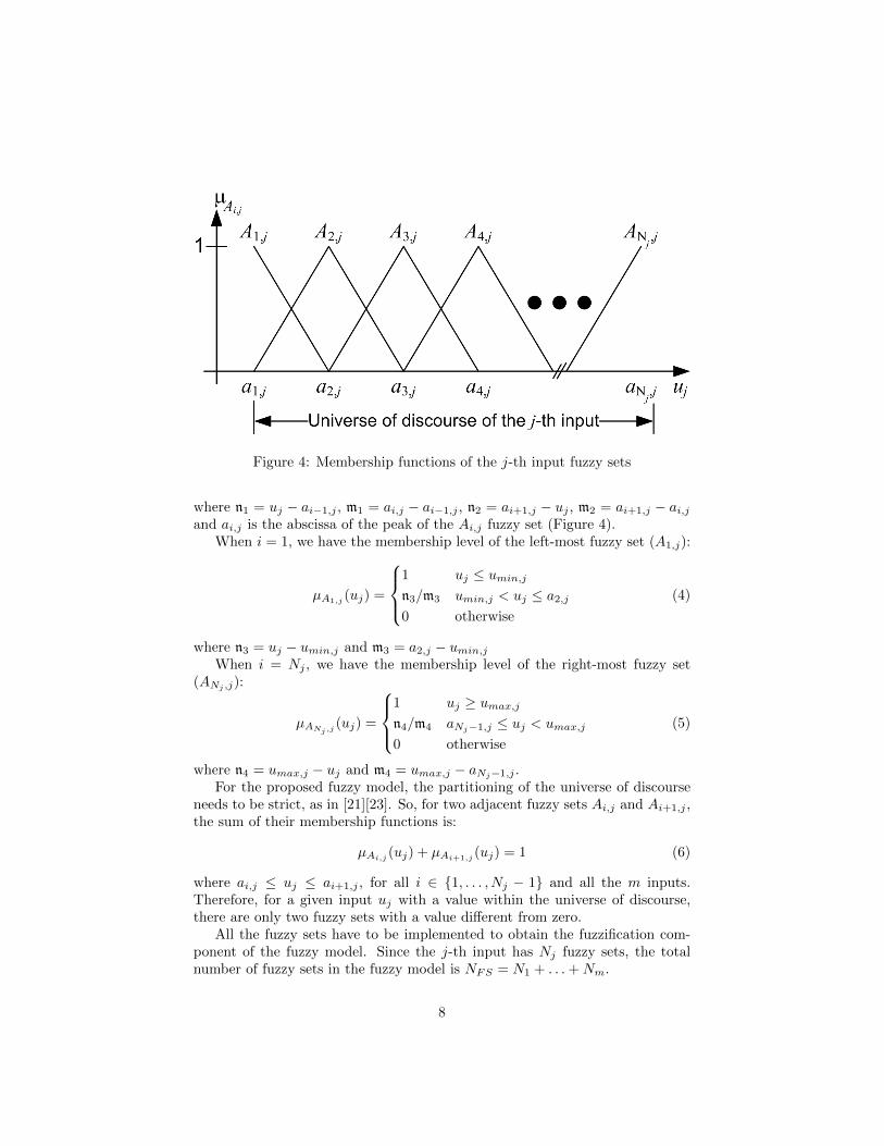
Figure 4: Membership functions of the j-th input fuzzy sets

where n1 = uj − ai−1,j , m1 = ai,j − ai−1,j , n2 = ai+1,j − uj , m2 = ai+1,j − ai,jand ai,j is the abscissa of the peak of the Ai,j fuzzy set (Figure 4).

When i = 1, we have the membership level of the left-most fuzzy set (A1,j):

µA1,j(uj) =

1 uj ≤ umin,j

n3/m3 umin,j < uj ≤ a2,j

0 otherwise

(4)

where n3 = uj − umin,j and m3 = a2,j − umin,j

When i = Nj , we have the membership level of the right-most fuzzy set(ANj ,j):

µANj,j(uj) =

1 uj ≥ umax,j

n4/m4 aNj−1,j ≤ uj < umax,j

0 otherwise

(5)

where n4 = umax,j − uj and m4 = umax,j − aNj−1,j .For the proposed fuzzy model, the partitioning of the universe of discourse

needs to be strict, as in [21][23]. So, for two adjacent fuzzy sets Ai,j and Ai+1,j ,the sum of their membership functions is:

µAi,j (uj) + µAi+1,j (uj) = 1 (6)

where ai,j ≤ uj ≤ ai+1,j , for all i ∈ {1, . . . , Nj − 1} and all the m inputs.Therefore, for a given input uj with a value within the universe of discourse,there are only two fuzzy sets with a value different from zero.

All the fuzzy sets have to be implemented to obtain the fuzzification com-ponent of the fuzzy model. Since the j-th input has Nj fuzzy sets, the totalnumber of fuzzy sets in the fuzzy model is NFS = N1 + . . .+Nm.

8

4.3 Defining the required input vectors necessary for ex-perimentation on the process

In fuzzy logic, each rule is associated with a combination of the fuzzy sets ofthe inputs. For example, rule Ri1,...,im,k is defined as follows:

Ri1,...,im,k : If u1 isAi1,1 and . . . and um isAim,m, then yk = ri1,...,im,k (7)

In (7), k is the output number, and ij ∈ {1, . . . , Nj} is used to identify the fuzzyset number considered in the rule for the j-th input. The consequent of ruleRi1,...,im,k is expressed by ri1,...,im,k. The k-th output yk is obtained from therules consequent.

In this paper, we propose to create the fuzzy model rules from a databasebuilt from experiments performed on the process. The input vectors (also calledinput tuples) used in the experiments are defined from the fuzzy sets definedin the previous step. In the input tuple, the j-th input uj is such that uj ∈{umin,j , b1,j , . . . , bNj−1,j , umax,j}, where the bi,j abscissa are:

bi,j = (ai,j + ai+1,j)/2, i ∈ {1, . . . , Nj − 1} (8)

and this is done for all the m inputs (j ∈ {1, . . . ,m}).The input tuples used to build the database are identified by the vector

θ{i1,...,im} where the indices ij ∈ {1, . . . , Nj + 1}.Since there are m inputs, the results of 2m experiments are required for

each rule. As the number of rules for the j-th input is defined as Nj , the totalnumber of rules required for each output is N = N1 × . . . × Nm. The totalnumber of experiments required to obtain all N rules of the fuzzy model isNexperiments = (N1 + 1) × . . . × (Nm + 1). The results of 2m experiments areused to obtain each rule.

4.3.1 Example

To help explain the notation, we consider a system with two inputs. Four (22)measurements are required to obtain rule R1,1,k, defined as:

R1,1,k : If u1 isA1,1 and u2 isA1,2, then yk = r1,1,k (9)

The input tuples applied to the system for those four measurements are: θ{1,1} =[umin,1 umin,2]T , θ{1,2} = [umin,1 b1,2]T , θ{2,1} = [b1,1 umin,2]T and θ{2,2} =[b1,1 b1,2]T . Then, the four experiments are performed by setting u = θ{i,j}with i, j ∈ {1, 2}. �

4.4 Building the rules from the database

All the experiments performed on the process provide a database linking themeasured output vectors φ{i1,...,im} ∈ Rm with each corresponding input vector(or tuple) θ{i1,...,im} ∈ Rm (with ij ∈ {1, . . . , Nj + 1}). The rules are obtainedfrom those experiments. The Rl1,...,lm,k rule of the k-th output is obtained from

9

the results of 2m experiments, where the corresponding input tuples are on thefollowing list:

{∀ θ{i1,...,im} | ij ∈ {lj , lj + 1}} (10)

and the corresponding k-th output measurements are also on this list:

{∀ φ{i1,...,im},k | ij ∈ {lj , lj + 1}} (11)

The cardinality of these two lists is 2m.The two lists, (10) and (11), are used to find the consequent rl1,...,lm,k of the

rule Rl1,...,lm,k by using kriging interpolation. The contents of the two lists arearranged in an m× 2m matrix defined as:

Θ{l1,...,lm} =[θ{l1,...,lm} . . . θ{l1+1,...,lm+1}

]T(12)

and the corresponding k-th output vector (of size 2m):

Y{l1,...,lm},k =[φ{l1,...,lm},k . . . φ{l1+1,...,lm+1},k

]T (13)

4.4.1 Example (con’t)

Continuing the example with two inputs, the matrices used to find the ruleR1,1,k are:

Θ{1,1} =[θ{1,1} θ{1,2} θ{2,1} θ{2,2}

]T(14)

and :

Y{1,1},k =[φ{1,1},k φ{1,2},k φ{2,1},k φ{2,2},k

]T (15)

�Kringing [25] is the approach used to perform the interpolation to obtain the

rules of the fuzzy model [26]. The equation used by the kriging interpolationto obtain the coefficients of the rule consequent rl1,...,lm,k is the following linearsystem: I2m 1T

2m Θ{l1,...,lm}12m 0 0m

ΘT{l1,...,lm} 0T

m 0m×m

×B{l1,...,lm},kc{l1,...,lm},0,kA{l1,...,lm},k

=

Y{l1,...,lm},k0

0m

(16)

In (16), I2m ∈ R2m×2m

represents the identity matrix, 0m×m ∈ Rm×m is asquare matrix filled with zeros, 12m ∈ R2m

is a vector filled with ones and0m ∈ Rm is a vector filled with zeros. The vector A{l1,...,lm},k ∈ Rm containsthe list of the coefficients of the rule consequent rl1,...,lm,k:

A{l1,...,lm},k =[c{l1,...,lm},1,k . . . c{l1,...,lm},m,k

]T(17)

10

The constant coefficient of the rule rl1,...,lm,k is the variable c{l1,...,lm},0,k. Fromthe coefficients contained in A{l1,...,lm},k and c{l1,...,lm},0,k, the rule consequentrl1,...,lm,k of a TSK FIS of order 1 is defined by this affine function:

rl1,...,lm,k = c{l1,...,lm},0,k +

m∑j=1

(c{l1,...,lm},j,k × uj

)(18)

The vector B{l1,...,lm},k ∈ R2m

contains the information about the interpo-lation accuracy [25]. When this vector is filled with zeros, the kriging interpola-tion gives the exact model for the subspace corresponding to the rule Ri1,...,im,k,based on the 2m measurements.

The coefficients of the rule Ri1,...,im,k and the vector B{l1,...,lm},k are ob-tained by solving the linear system (16). This interpolation process is repeatedN ×m times, since there are N rules consequent for each of the m outputs.

From the interpolated rule consequent ri1,...,im,k, we are able to build vectorsand matrices. In fact, the rule consequents are grouped into vectors R{l1,...,lm} ∈Rm as follows:

R{l1,...,lm} =[rl1,...,lm,1 . . . rl1,...,lm,m

]T(19)

and each of these vectors is defined as follows:

R{l1,...,lm} = C{l1,...,lm} + DT{l1,...,lm}u (20)

In (20), C{l1,...,lm} ∈ Rm is a vector containing the c{l1,...,lm},0,k terms of therules:

C{l1,...,lm} =[c{l1,...,lm},0,1 . . . c{l1,...,lm},0,m

]T(21)

and D{l1,...,lm} ∈ Rm×m is a matrix containing the c{l1,...,lm},j,k terms (withj 6= 0) of the rules:

D{l1,...,lm} =

c{l1,...,lm},1,1 . . . c{l1,...,lm},m,1

.... . .

...c{l1,...,lm},1,m . . . c{l1,...,lm},m,m

(22)

All the inputs of the fuzzy model are combined into a vector u = [u1, . . . , um]T ∈Rm.

As the kriging interpolation is linear, it is possible to obtain the matrix Dand the vector C defined in (22) and (21) directly, since it is possible to rewrite(16) as follows: I2m 1T

2m Θ{l1,...,lm}12m 0 0m

ΘT{l1,...,lm} 0T

m 0m×m

× B{l1,...,lm}

CT{l1,...,lm}

DT{l1,...,lm}

=

Y{l1,...,lm}0

0m

(23)

where the matrices B{l1,...,lm} ∈ Rm×2m

and Y{l1,...,lm} ∈ Rm×2m

are respec-tively:

B{l1,...,lm} =[

B{l1,...,lm,},1 . . . B{l1,...,lm,},m]

(24)

11

andY{l1,...,lm} =

[Y{l1,...,lm,},1 . . . Y{l1,...,lm,},m

](25)

By solving the linear system defined in (23), the vector C{l1,...,lm,} and thematrix D{l1,...,lm,} are calculated directly.

When the rule consequent are represented vectorially, the Ri1,...,im,k rules,defined in (7) with k ∈ {1, . . . ,m}, are combined into this rule:

Ri1,...,im : If u1 isAi1,1 and . . . and um isAim,m, then y = R{i1,...,im} (26)

with R{i1,...,im} defined in (20) and the output vector y = [y1 . . . ym]T ∈ Rm.This vectorial representation of the rule consequent simplifies the represen-

tation of the FIS rules and the inversion of the rules to obtain the inverse fuzzymodel.

4.5 The resulting fuzzy model

By following the steps presented in the above section, a fuzzy model based onthe TSK FIS of order 1 is obtained. To implement this model, Nj fuzzy setsmust be defined for the j-th input – see equations (3) to (5). This means thatthere are N rules to define per output, resulting in N linear equations - see (20).

In the next section, the inversion of this fuzzy model is introduced.

5 Inversion of the fuzzy model

To design the fuzzy TILC algorithm, the fuzzy model of the MIMO process hasto be inverted. Two steps are required to achieve this. The first step is to definethe fuzzy sets of the inputs of the inverse fuzzy model from the fuzzy sets ofthe inputs of the fuzzy model. If this first step is feasible, the second step is toobtain the rule consequents of the inverse fuzzy model from the rule consequentof the fuzzy model.

5.1 Preliminary assumptions

Before explaining the inversion of the fuzzy model, we must state the followingtwo assumptions about the TSK fuzzy model that will be inverted.

Assumption III-1 That the number of inputs is equal to the number ofoutputs, or p = m, and also that input ui is paired with output yi in the fuzzymodel. This assumption is not very restrictive, since the input output pairingof a MIMO process can be achieved using an approach like Relative Gain Array(RGA) [27]. Once this pairing has been made, the outputs are renamed, suchthat output yi is paired with input ui.

12

a)

b)

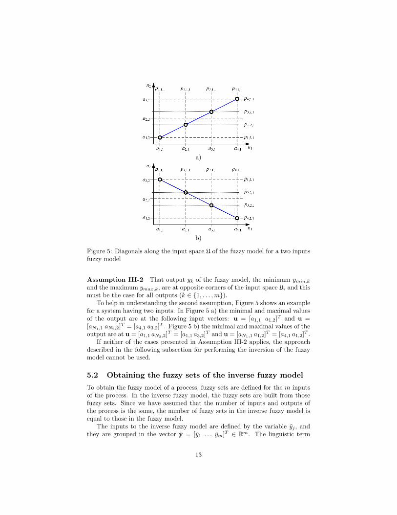
Figure 5: Diagonals along the input space U of the fuzzy model for a two inputsfuzzy model

Assumption III-2 That output yk of the fuzzy model, the minimum ymin,k

and the maximum ymax,k, are at opposite corners of the input space U, and thismust be the case for all outputs (k ∈ {1, . . . ,m}).

To help in understanding the second assumption, Figure 5 shows an examplefor a system having two inputs. In Figure 5 a) the minimal and maximal valuesof the output are at the following input vectors: u = [a1,1 a1,2]T and u =[aN1,1 aN2,2]T = [a4,1 a3,2]T . Figure 5 b) the minimal and maximal values of theoutput are at u = [a1,1 aN2,2]T = [a1,1 a3,2]T and u = [aN1,1 a1,2]T = [a4,1 a1,2]T .

If neither of the cases presented in Assumption III-2 applies, the approachdescribed in the following subsection for performing the inversion of the fuzzymodel cannot be used.

5.2 Obtaining the fuzzy sets of the inverse fuzzy model

To obtain the fuzzy model of a process, fuzzy sets are defined for the m inputsof the process. In the inverse fuzzy model, the fuzzy sets are built from thosefuzzy sets. Since we have assumed that the number of inputs and outputs ofthe process is the same, the number of fuzzy sets in the inverse fuzzy model isequal to those in the fuzzy model.

The inputs to the inverse fuzzy model are defined by the variable yj , andthey are grouped in the vector y = [y1 . . . ym]T ∈ Rm. The linguistic term

13

of the i-th fuzzy set of k-input yk of the inverse fuzzy model is identified byAi,k. The coordinates of the peak of each of those fuzzy sets are identified byai,k. Each of the ai,k coordinates is calculated from the ai,j coordinates fromthe fuzzy model in a two steps process.

To explain this process, let us consider a two input, two output fuzzy model.Figure 5 shows the universe of discourse of both the inputs and the coordinates(ai,j) of the peaks of the fuzzy sets of both the inputs. The output y1 of thisfuzzy model is assumed to be minimal when input u1 = a1,1 and input u2 = a1,2,and maximal when u1 = a4,1 and u2 = a3,2.

Each of the peaks ai,1 of the fuzzy sets Ai,1 of the input y1 of the inversefuzzy model is obtained as follows:

First, the coordinates pi,j,k, where the fuzzy sets of the input u1 have theirpeaks, are calculated. Then, for this input, the coordinates pi,1,1 are the coordi-nates ai,1 directly, and so pi,1,1 = ai,1. For the other input (u2), the coordinatesto consider are identified as pi,2,1, and are calculated by the equations below(when j 6= k).

For case A in Figure 5:

pi,j,k =(aNj ,j − a1,j)

(aNk,k − a1,k)(ai,k − a1,k) + a1,j

=(umax,j − umin,j)

(umax,k − umin,k)(ai,k − umin,k) + umin,j

(27)

and for case B in Figure 5:

pi,j,k =(aNj ,j − a1,j)

(aNk,k − a1,k)(aNk,k − ai,k) + a1,j

=(umax,j − umin,j)

(umax,k − umin,k)(umax,k − ai,k) + umin,j

(28)

In both cases, when j = k (the number of inputs and outputs is the same),the equation to use is pi,k,k = ai,k.

Finally, the coordinates ai,k are obtained directly from the evaluation of thefuzzy model with the input vector built from those pi,j,k values. So, ai,k isdirectly, the k-th output value yk of the fuzzy model with the vector [pi,1,k . . .pi,m,k]T applied as the input vector.

In this paper, we consider the following two cases. If ai,k are not increasing,then a1,k ≤ a2,k ≤ . . . ≤ aNk,k. If ai,k are not decreasing, then a1,k ≥ a2,k ≥. . . ≥ aNk,k. We check for all k (or all input output pairs), if either case applies.If neither of these two cases applies, the approach presented in this paper cannotbe used. In this situation, it is not possible to design a TILC algorithm basedon the inverse of the fuzzy model.

14

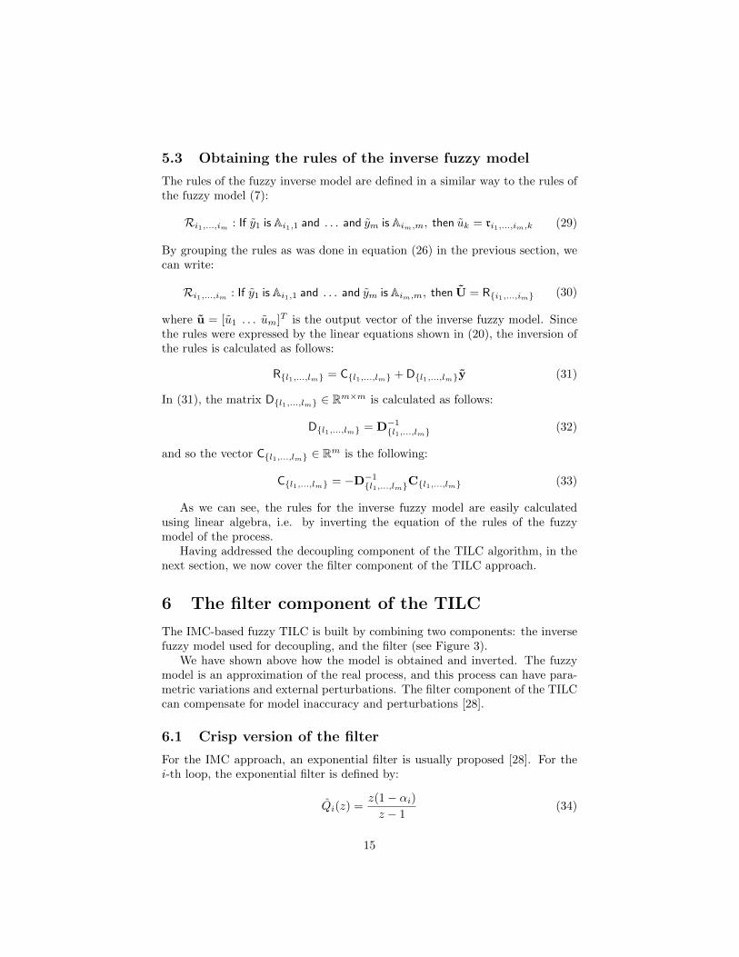
5.3 Obtaining the rules of the inverse fuzzy model

The rules of the fuzzy inverse model are defined in a similar way to the rules ofthe fuzzy model (7):

Ri1,...,im : If y1 is Ai1,1 and . . . and ym is Aim,m, then uk = ri1,...,im,k (29)

By grouping the rules as was done in equation (26) in the previous section, wecan write:

Ri1,...,im : If y1 is Ai1,1 and . . . and ym is Aim,m, then U = R{i1,...,im} (30)

where u = [u1 . . . um]T is the output vector of the inverse fuzzy model. Sincethe rules were expressed by the linear equations shown in (20), the inversion ofthe rules is calculated as follows:

R{l1,...,lm} = C{l1,...,lm} + D{l1,...,lm}y (31)

In (31), the matrix D{l1,...,lm} ∈ Rm×m is calculated as follows:

D{l1,...,lm} = D−1{l1,...,lm} (32)

and so the vector C{l1,...,lm} ∈ Rm is the following:

C{l1,...,lm} = −D−1{l1,...,lm}C{l1,...,lm} (33)

As we can see, the rules for the inverse fuzzy model are easily calculatedusing linear algebra, i.e. by inverting the equation of the rules of the fuzzymodel of the process.

Having addressed the decoupling component of the TILC algorithm, in thenext section, we now cover the filter component of the TILC approach.

6 The filter component of the TILC

The IMC-based fuzzy TILC is built by combining two components: the inversefuzzy model used for decoupling, and the filter (see Figure 3).

We have shown above how the model is obtained and inverted. The fuzzymodel is an approximation of the real process, and this process can have para-metric variations and external perturbations. The filter component of the TILCcan compensate for model inaccuracy and perturbations [28].

6.1 Crisp version of the filter

For the IMC approach, an exponential filter is usually proposed [28]. For thei-th loop, the exponential filter is defined by:

Qi(z) =z(1− αi)

z − 1(34)

15

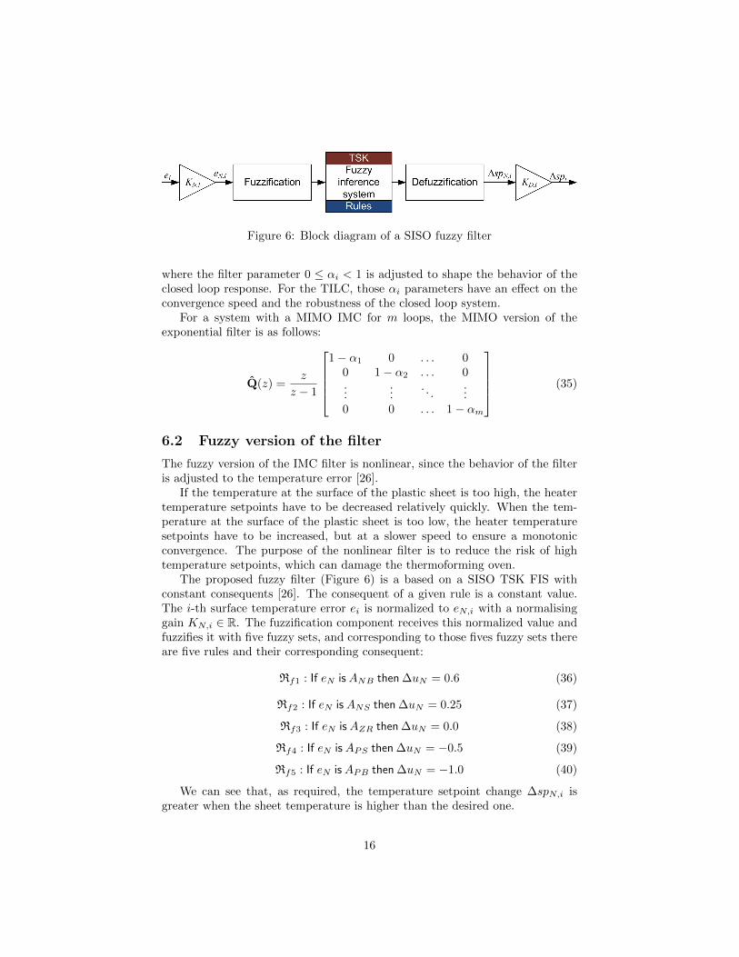
Figure 6: Block diagram of a SISO fuzzy filter

where the filter parameter 0 ≤ αi < 1 is adjusted to shape the behavior of theclosed loop response. For the TILC, those αi parameters have an effect on theconvergence speed and the robustness of the closed loop system.

For a system with a MIMO IMC for m loops, the MIMO version of theexponential filter is as follows:

Q(z) =z

z − 1

1− α1 0 . . . 0

0 1− α2 . . . 0...

.... . .

...0 0 . . . 1− αm

(35)

6.2 Fuzzy version of the filter

The fuzzy version of the IMC filter is nonlinear, since the behavior of the filteris adjusted to the temperature error [26].

If the temperature at the surface of the plastic sheet is too high, the heatertemperature setpoints have to be decreased relatively quickly. When the tem-perature at the surface of the plastic sheet is too low, the heater temperaturesetpoints have to be increased, but at a slower speed to ensure a monotonicconvergence. The purpose of the nonlinear filter is to reduce the risk of hightemperature setpoints, which can damage the thermoforming oven.

The proposed fuzzy filter (Figure 6) is a based on a SISO TSK FIS withconstant consequents [26]. The consequent of a given rule is a constant value.The i-th surface temperature error ei is normalized to eN,i with a normalisinggain KN,i ∈ R. The fuzzification component receives this normalized value andfuzzifies it with five fuzzy sets, and corresponding to those fives fuzzy sets thereare five rules and their corresponding consequent:

Rf1 : If eN isANB then ∆uN = 0.6 (36)

Rf2 : If eN isANS then ∆uN = 0.25 (37)

Rf3 : If eN isAZR then ∆uN = 0.0 (38)

Rf4 : If eN isAPS then ∆uN = −0.5 (39)

Rf5 : If eN isAPB then ∆uN = −1.0 (40)

We can see that, as required, the temperature setpoint change ∆spN,i isgreater when the sheet temperature is higher than the desired one.

16

The rule consequent are defuzzified, and the resulting value is defuzzifiedwith the gain KD,i ∈ R and denormalized to obtain the i-th output value ∆spi.Then, the output of the filter is, finally: spi[k + 1] = spi[k] + ∆spi[k]. Thisoutput is sent to the fuzzy inverse model to generate the heater temperaturesetpoints.

The initial value spi[0] (for cycle k = 0) of the fuzzy filter is equal to thedesired terminal temperature yd,i. These initial values (∀i ∈ {1, . . . ,m}) will beused to calculate the initial guess for the heater temperature setpoints.

7 Application to a thermoforming machine

The fuzzy TILC design approach presented in this paper is now applied to anonlinear model of a thermoforming machine. This model, presented briefly inthe Appendix, is based on the AAA thermoforming machine [12]. The simu-lated thermoforming machine has six inputs (heaters) and six outputs (infra-redsensors).

The six heaters are obtained by grouping the heaters bank (see Figure 7)as follows: T1-T4, T2-T5, T3-T6, B1-B4, B2-B5, and B3-B6 (T identifies a topheater, and B identifies a bottom heater). Furthermore, the system input vectoru ∈ R6 is defined as follows:

u =

u1

u2

u3

u4

u5

u6

=

T2 − T5

T1 − T4

T3 − T6

B2 −B5

B1 −B4

B3 −B6

(41)

The six infrared (IR) sensors selected are (see Figure 7): IRT1, IRT2, IRT5,IRB1, IRB2, and IRB5 (again, T identifies a top IR sensor, B identifies abottom IR sensor). So, the model output vector y ∈ R6 is defined as follows:

y =

y1

y2

y3

y4

y5

y6

=

IRT1

IRT2

IRT5

IRB1

IRB2

IRB5

(42)

7.1 Simulation setup

The objective of the controllers is to maintain the terminal surface temperatureerror within a 5◦C range. However, a 10◦C error is considered acceptable forquality control.

The thermoforming model is used as benchmark to test the following threeTILC algorithms:

17

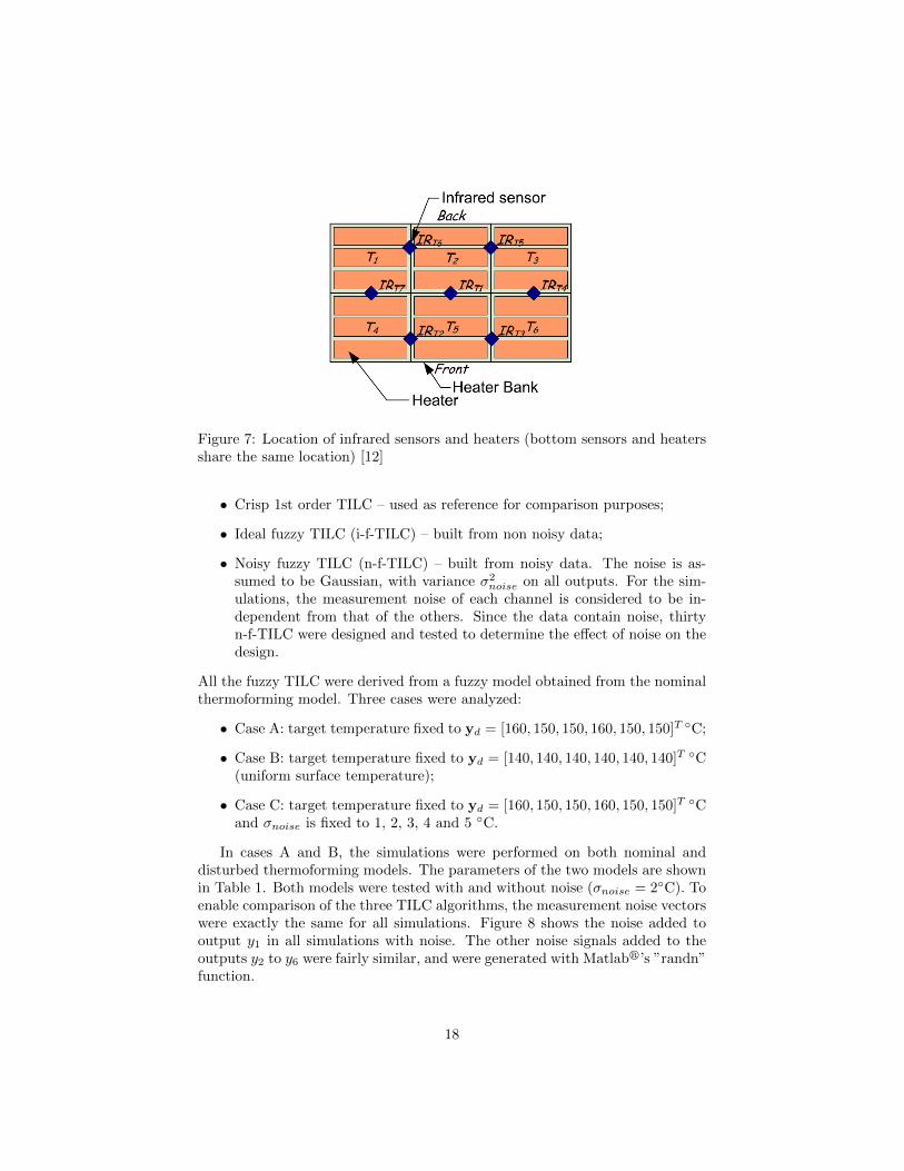
Figure 7: Location of infrared sensors and heaters (bottom sensors and heatersshare the same location) [12]

• Crisp 1st order TILC – used as reference for comparison purposes;

• Ideal fuzzy TILC (i-f-TILC) – built from non noisy data;

• Noisy fuzzy TILC (n-f-TILC) – built from noisy data. The noise is as-sumed to be Gaussian, with variance σ2

noise on all outputs. For the sim-ulations, the measurement noise of each channel is considered to be in-dependent from that of the others. Since the data contain noise, thirtyn-f-TILC were designed and tested to determine the effect of noise on thedesign.

All the fuzzy TILC were derived from a fuzzy model obtained from the nominalthermoforming model. Three cases were analyzed:

• Case A: target temperature fixed to yd = [160, 150, 150, 160, 150, 150]T ◦C;

• Case B: target temperature fixed to yd = [140, 140, 140, 140, 140, 140]T ◦C(uniform surface temperature);

• Case C: target temperature fixed to yd = [160, 150, 150, 160, 150, 150]T ◦Cand σnoise is fixed to 1, 2, 3, 4 and 5 ◦C.

In cases A and B, the simulations were performed on both nominal anddisturbed thermoforming models. The parameters of the two models are shownin Table 1. Both models were tested with and without noise (σnoise = 2◦C). Toenable comparison of the three TILC algorithms, the measurement noise vectorswere exactly the same for all simulations. Figure 8 shows the noise added tooutput y1 in all simulations with noise. The other noise signals added to theoutputs y2 to y6 were fairly similar, and were generated with Matlabr’s ”randn”function.

18

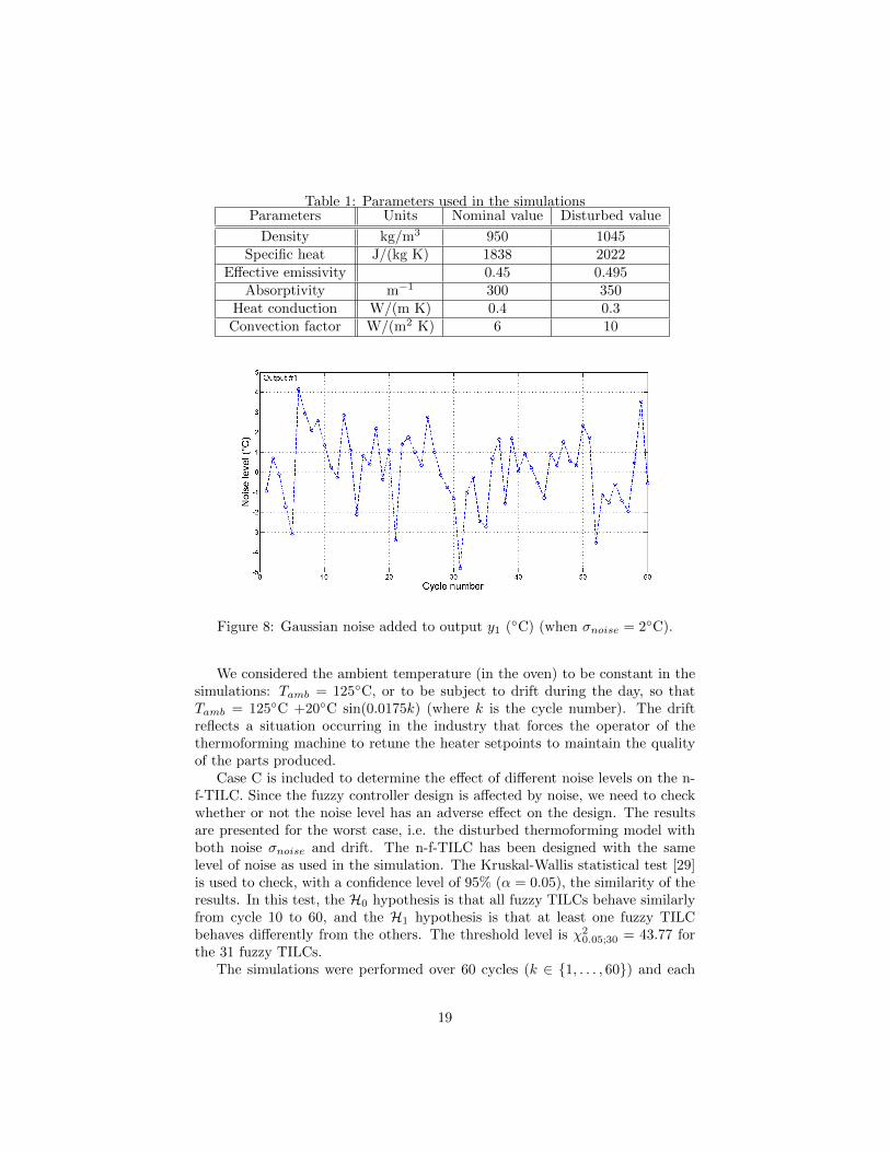
Table 1: Parameters used in the simulationsParameters Units Nominal value Disturbed value

Density kg/m3 950 1045Specific heat J/(kg K) 1838 2022

Effective emissivity 0.45 0.495Absorptivity m−1 300 350

Heat conduction W/(m K) 0.4 0.3Convection factor W/(m2 K) 6 10

Figure 8: Gaussian noise added to output y1 (◦C) (when σnoise = 2◦C).

We considered the ambient temperature (in the oven) to be constant in thesimulations: Tamb = 125◦C, or to be subject to drift during the day, so thatTamb = 125◦C +20◦C sin(0.0175k) (where k is the cycle number). The driftreflects a situation occurring in the industry that forces the operator of thethermoforming machine to retune the heater setpoints to maintain the qualityof the parts produced.

Case C is included to determine the effect of different noise levels on the n-f-TILC. Since the fuzzy controller design is affected by noise, we need to checkwhether or not the noise level has an adverse effect on the design. The resultsare presented for the worst case, i.e. the disturbed thermoforming model withboth noise σnoise and drift. The n-f-TILC has been designed with the samelevel of noise as used in the simulation. The Kruskal-Wallis statistical test [29]is used to check, with a confidence level of 95% (α = 0.05), the similarity of theresults. In this test, the H0 hypothesis is that all fuzzy TILCs behave similarlyfrom cycle 10 to 60, and the H1 hypothesis is that at least one fuzzy TILCbehaves differently from the others. The threshold level is χ2

0.05;30 = 43.77 forthe 31 fuzzy TILCs.

The simulations were performed over 60 cycles (k ∈ {1, . . . , 60}) and each

19

cycle corresponded to 12 mm plastic sheets being heated for 300 seconds (5minutes).

7.2 Parameters for obtaining the inverse fuzzy model

The fuzzy models of the thermoforming machine were developed by defining auniverse of discourse for each input, where umin,k = 300◦C and umax,k = 450◦C(with k ∈ {1, . . . , 6}). Each universe of discourse is divided among three fuzzysets with the peaks located at: a1,k = 300◦C, a2,k = 375◦C and a1,k = 450◦C(with k ∈ {1, . . . , 6}) respectively.

There are 36 = 729 rules for obtaining each output. This requires 46 = 4096experiments (simulations, here) to be performed on the thermoforming machinemodel.

The inverse of the fuzzy model involves evaluating the universe of discourseof all the outputs. The lower limits of those universes of discourse are ob-tained when all six heating elements are at the lowest setpoint: 300◦C. Withoutmeasurement noise (and nominal parameters), those lower limits are: ymin,k =105.06◦C (for k = 1, 3, 4, 6) and ymin,k = 117.03◦C (for k = 2, 5). The higherlimits are obtained when all the heating elements are at the highest setpoint:450◦C. Again, with no measurement noise, these limits are: ymax,k = 203.89◦C(for k = 1, 3, 4, 6) and ymax,k = 233.30◦C (for k = 2, 5). So, as assumed, theminimum and maximum output temperatures are at opposite sides of the inputspace U. Since the inputs of the fuzzy model were fuzzified with three fuzzy setseach, the same applies to the inputs of the inverse fuzzy model.

All the fuzzy filters of the fuzzy TILC have normalization gains KN,i = 0.25and denormalization gains KD,i = 1.00 for i ∈ {1, . . . , 6}.

The two fuzzy TILCs are compared with a so-called crisp TILC based on alinear IMC approach, with an exponential filter [12][28] where the parametersare αi = 0.2701 ∀i ∈ {1, . . . , 6}.

7.3 Simulation results

The simulation results are presented below to compare the behavior of the threeTILCs in different situations.

7.3.1 Case A

The first set of simulations has a target temperature vector yd = [160, 150, 150,160, 150, 150]T ◦C. The heater temperature setpoints used for the crisp TILC atcycle k = 1 are arbitrarily fixed to 350◦C for all the heaters. This value is a badguess, as shown by the surface temperature error at cycle k = 1 (or ||e[1]||∞)displayed in last column of Tables 2, 3, 4 and 5. It is to be hoped that the crispTILC algorithm will reduce this error to a lower level as the cycle number kincreases. In the ideal case (no noise and no drift), the error converges to zero.

For the two fuzzy TILCs, the initial heater temperature setpoints are ob-tained from the inverse fuzzy model. With the i-f-TILC, the first heater tem-

20

perature setpoints are in the vector sp = [399.97, 353.22, 403.16, 399.97, 353.22,403.16]T ◦C. As shown in Tables 2 to 5, the surface temperature error obtainedin the first cycle or ||e[1]||∞ is lower than the error obtained with the crispTILC. Since 30 n-f-TILCs were tested, the values displayed are the mean of the30 n-f-TILC guesses. The differences between the initial setpoint evaluated bythe i-f-TILCs and those evaluated by the 30 n-f-TILCs seem to be negligible.

TILC algorithms must converge to a setpoint vector sp, such that the surfacetemperature error ||e[k]||∞ falls to 0. When there is no noise, all TILC errorsconverge to 0. But, when there is noise, there is an error (see µe and σe in Tables3 to 5). µe is the mean error during cycles 10 to 60, and σe is the standarddeviation associated with this mean.

Table 2: Simulation results (Case A) — without noise and driftTILC algorithm System ||e[1]||∞ (◦C)

Crisp TILCDisturbed 20.7607Nominal 18.8756

i-f-TILCDisturbed 5.5493Nominal 1.0671

n-f-TILC Disturbed 5.8967(mean of 30 controllers) Nominal 1.5671

As shown in Table 3, when there is noise (σnoise = 2◦C), both fuzzy TILCsoutperform the crisp TILC by nearly 1.25◦C, and the standard deviation σe ofthe surface temperature error is divided by 1.5.

Table 3: Simulation results (Case A) — with noise (µe and σe for k ∈{10, . . . , 60})

TILC algorithm System µe (◦C) σe (◦C) ||e[1]||∞ (◦C)

Crisp TILCDisturbed 5.1039 1.6734 26.6153Nominal 4.9209 1.5830 24.7302

i-f-TILCDisturbed 3.8572 1.0799 10.5062Nominal 3.6603 1.0521 6.9217

n-f-TILC Disturbed 3.8653 1.0887 10.4140(mean of 30 controllers) Nominal 3.6643 1.0539 6.8224

When the ambient temperature is subject to drift and no measurement noise,there is a small error (Table 4). This slowly varying error remains low, and thecrisp TILC gives a lower steady state error than either of the fuzzy TILCs.

Table 5 shows the results when we have both noise and drift. The resultslook similar to the results in Table 3. The drift effect seems relatively smallcompared to the noise effect. Figure 9 shows the worst case, when the systemis subjected to noise, drift, and parameter disturbance. This figure shows thatonce the TILC algorithms have converged, all the surface temperature errorsremain under 12◦C. Furthermore, the #1 n-f-TILC’s error remains below 6◦C

21

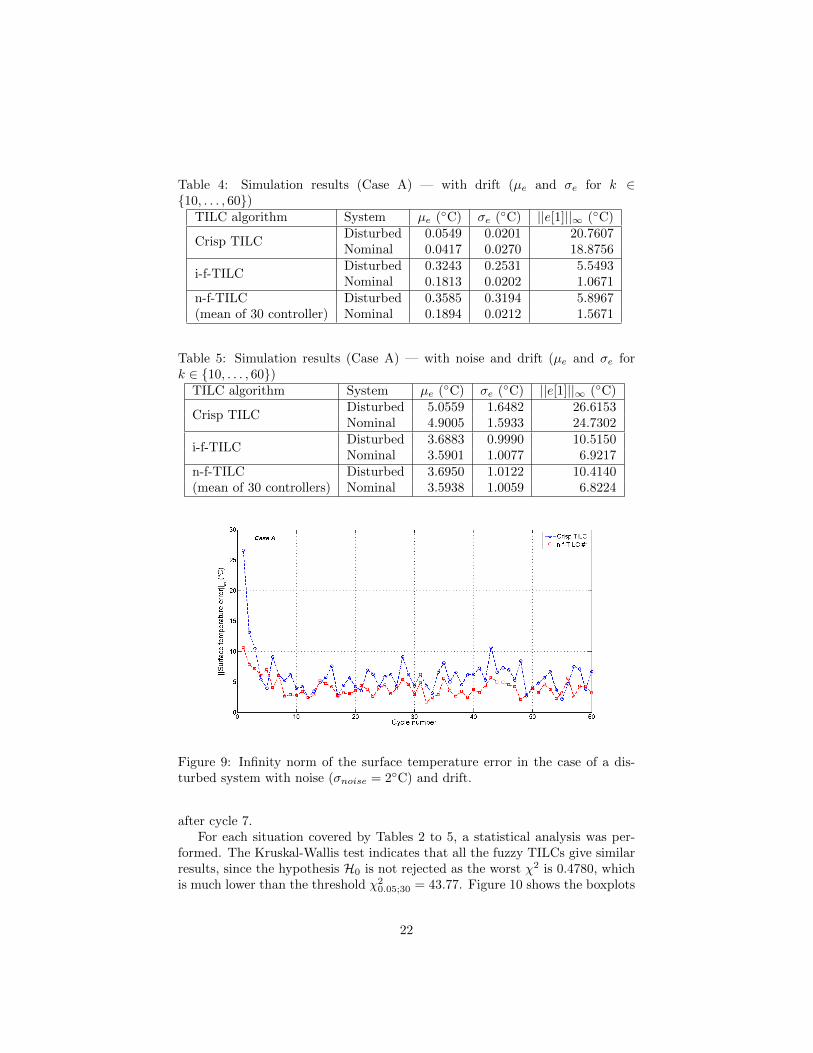
Table 4: Simulation results (Case A) — with drift (µe and σe for k ∈{10, . . . , 60})

TILC algorithm System µe (◦C) σe (◦C) ||e[1]||∞ (◦C)

Crisp TILCDisturbed 0.0549 0.0201 20.7607Nominal 0.0417 0.0270 18.8756

i-f-TILCDisturbed 0.3243 0.2531 5.5493Nominal 0.1813 0.0202 1.0671

n-f-TILC Disturbed 0.3585 0.3194 5.8967(mean of 30 controller) Nominal 0.1894 0.0212 1.5671

Table 5: Simulation results (Case A) — with noise and drift (µe and σe fork ∈ {10, . . . , 60})

TILC algorithm System µe (◦C) σe (◦C) ||e[1]||∞ (◦C)

Crisp TILCDisturbed 5.0559 1.6482 26.6153Nominal 4.9005 1.5933 24.7302

i-f-TILCDisturbed 3.6883 0.9990 10.5150Nominal 3.5901 1.0077 6.9217

n-f-TILC Disturbed 3.6950 1.0122 10.4140(mean of 30 controllers) Nominal 3.5938 1.0059 6.8224

Figure 9: Infinity norm of the surface temperature error in the case of a dis-turbed system with noise (σnoise = 2◦C) and drift.

after cycle 7.For each situation covered by Tables 2 to 5, a statistical analysis was per-

formed. The Kruskal-Wallis test indicates that all the fuzzy TILCs give similarresults, since the hypothesis H0 is not rejected as the worst χ2 is 0.4780, whichis much lower than the threshold χ2

0.05;30 = 43.77. Figure 10 shows the boxplots

22

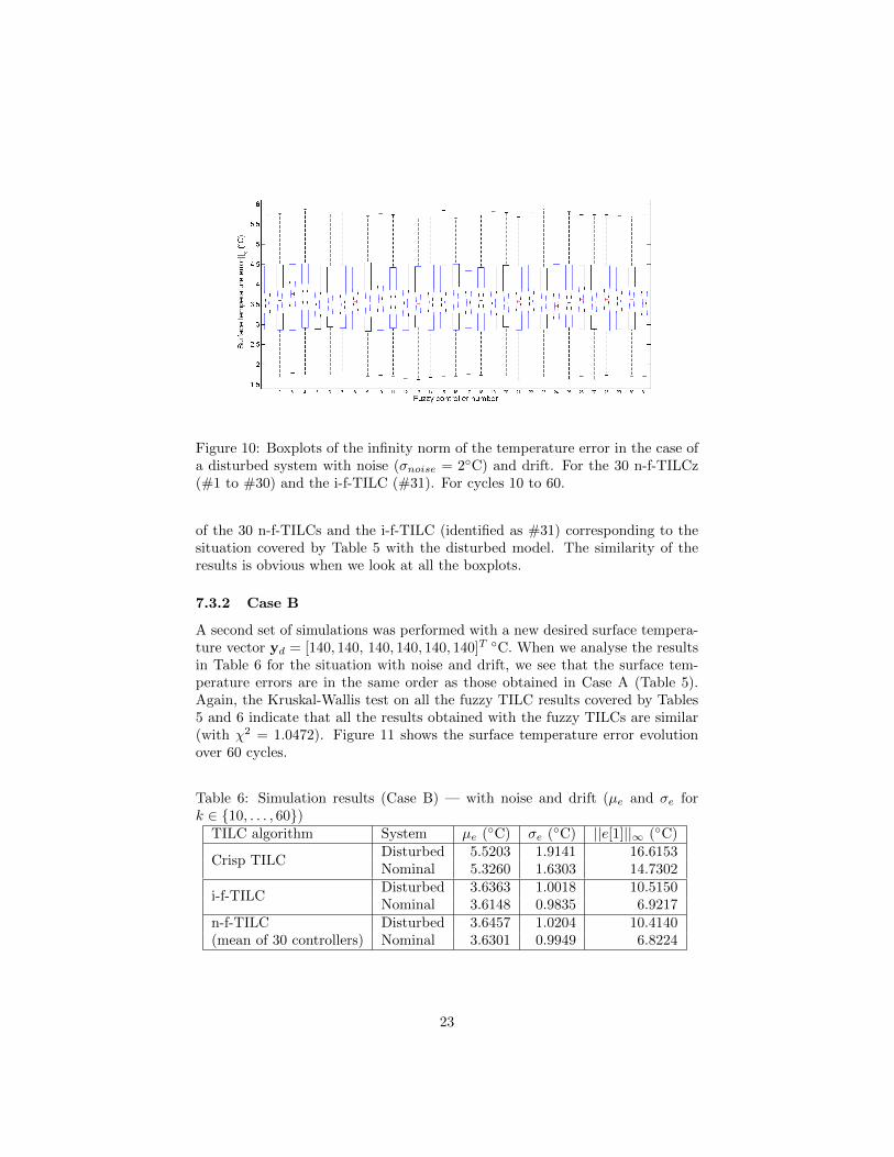
Figure 10: Boxplots of the infinity norm of the temperature error in the case ofa disturbed system with noise (σnoise = 2◦C) and drift. For the 30 n-f-TILCz(#1 to #30) and the i-f-TILC (#31). For cycles 10 to 60.

of the 30 n-f-TILCs and the i-f-TILC (identified as #31) corresponding to thesituation covered by Table 5 with the disturbed model. The similarity of theresults is obvious when we look at all the boxplots.

7.3.2 Case B

A second set of simulations was performed with a new desired surface tempera-ture vector yd = [140, 140, 140, 140, 140, 140]T ◦C. When we analyse the resultsin Table 6 for the situation with noise and drift, we see that the surface tem-perature errors are in the same order as those obtained in Case A (Table 5).Again, the Kruskal-Wallis test on all the fuzzy TILC results covered by Tables5 and 6 indicate that all the results obtained with the fuzzy TILCs are similar(with χ2 = 1.0472). Figure 11 shows the surface temperature error evolutionover 60 cycles.

Table 6: Simulation results (Case B) — with noise and drift (µe and σe fork ∈ {10, . . . , 60})

TILC algorithm System µe (◦C) σe (◦C) ||e[1]||∞ (◦C)

Crisp TILCDisturbed 5.5203 1.9141 16.6153Nominal 5.3260 1.6303 14.7302

i-f-TILCDisturbed 3.6363 1.0018 10.5150Nominal 3.6148 0.9835 6.9217

n-f-TILC Disturbed 3.6457 1.0204 10.4140(mean of 30 controllers) Nominal 3.6301 0.9949 6.8224

23

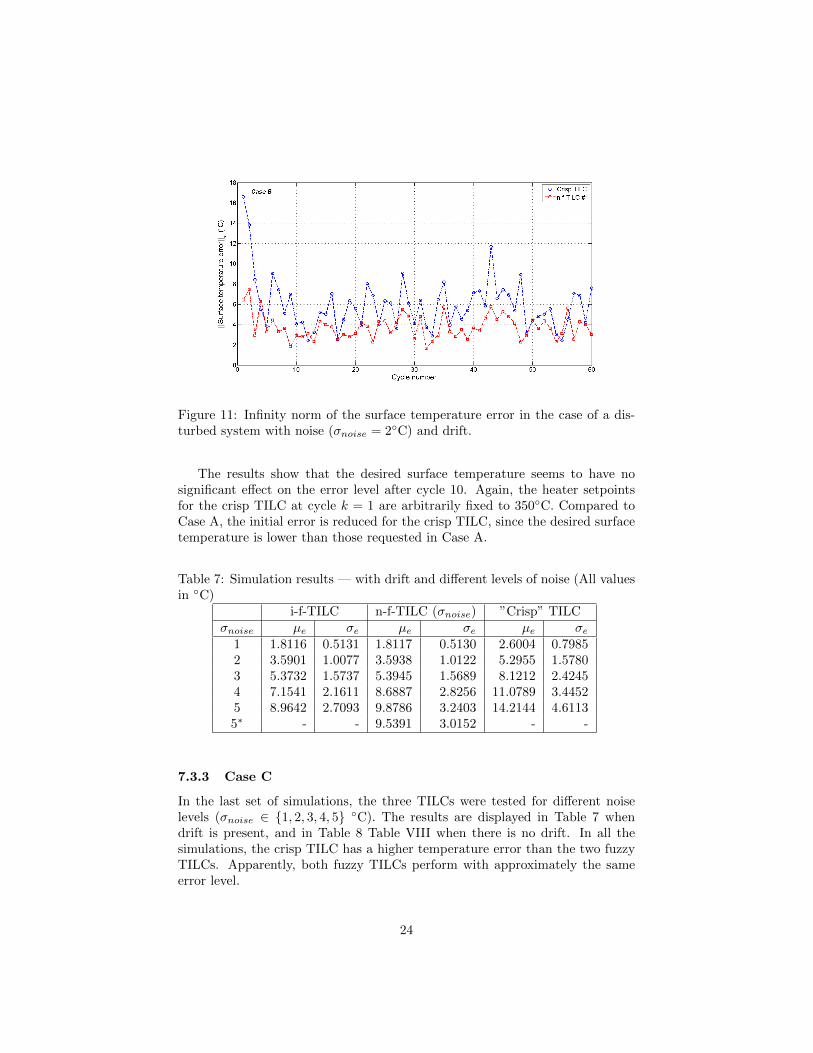
Figure 11: Infinity norm of the surface temperature error in the case of a dis-turbed system with noise (σnoise = 2◦C) and drift.

The results show that the desired surface temperature seems to have nosignificant effect on the error level after cycle 10. Again, the heater setpointsfor the crisp TILC at cycle k = 1 are arbitrarily fixed to 350◦C. Compared toCase A, the initial error is reduced for the crisp TILC, since the desired surfacetemperature is lower than those requested in Case A.

Table 7: Simulation results — with drift and different levels of noise (All valuesin ◦C)

i-f-TILC n-f-TILC (σnoise) ”Crisp” TILCσnoise µe σe µe σe µe σe

1 1.8116 0.5131 1.8117 0.5130 2.6004 0.79852 3.5901 1.0077 3.5938 1.0122 5.2955 1.57803 5.3732 1.5737 5.3945 1.5689 8.1212 2.42454 7.1541 2.1611 8.6887 2.8256 11.0789 3.44525 8.9642 2.7093 9.8786 3.2403 14.2144 4.61135∗ - - 9.5391 3.0152 - -

7.3.3 Case C

In the last set of simulations, the three TILCs were tested for different noiselevels (σnoise ∈ {1, 2, 3, 4, 5} ◦C). The results are displayed in Table 7 whendrift is present, and in Table 8 Table VIII when there is no drift. In all thesimulations, the crisp TILC has a higher temperature error than the two fuzzyTILCs. Apparently, both fuzzy TILCs perform with approximately the sameerror level.

24

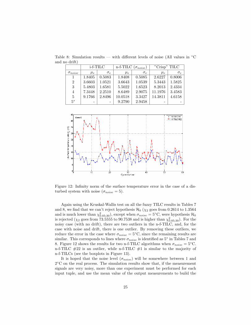
Table 8: Simulation results — with different levels of noise (All values in ◦Cand no drift)

i-f-TILC n-f-TILC (σnoise) ”Crisp” TILCσnoise µe σe µe σe µe σe

1 1.8405 0.5083 1.8408 0.5085 2.6227 0.80062 3.6603 1.0521 3.6643 1.0539 5.3443 1.58253 5.4803 1.6581 5.5022 1.6523 8.2013 2.43344 7.3448 2.2510 8.6489 2.9075 11.1976 3.45835 9.1766 2.8496 10.0518 3.3427 14.3811 4.61585∗ - - 9.2790 2.9458 - -

Figure 12: Infinity norm of the surface temperature error in the case of a dis-turbed system with noise (σnoise = 5).

Again using the Kruskal-Wallis test on all the fuzzy TILC results in Tables 7and 8, we find that we can’t reject hypothesis H0 (χ2 goes from 0.2614 to 1.3564and is much lower than χ2

0.05;30), except when σnoise = 5◦C, were hypothesis H0

is rejected (χ2 goes from 73.5555 to 90.7538 and is higher than χ20.05;30). For the

noisy case (with no drift), there are two outliers in the n-f-TILC, and, for thecase with noise and drift, there is one outlier. By removing these outliers, wereduce the error in the case where σnoise = 5◦C, since the remaining results aresimilar. This corresponds to lines where σnoise is identified as 5∗ in Tables 7 and8. Figure 12 shows the results for two n-f-TILC algorithms when σnoise = 5◦C.n-f-TILC #22 is an outlier, while n-f-TILC #1 is similar to the majority ofn-f-TILCs (see the boxplots in Figure 13).

It is hoped that the noise level (σnoise) will be somewhere between 1 and2◦C on the real process. The simulation results show that, if the measurementsignals are very noisy, more than one experiment must be performed for eachinput tuple, and use the mean value of the output measurements to build the

25

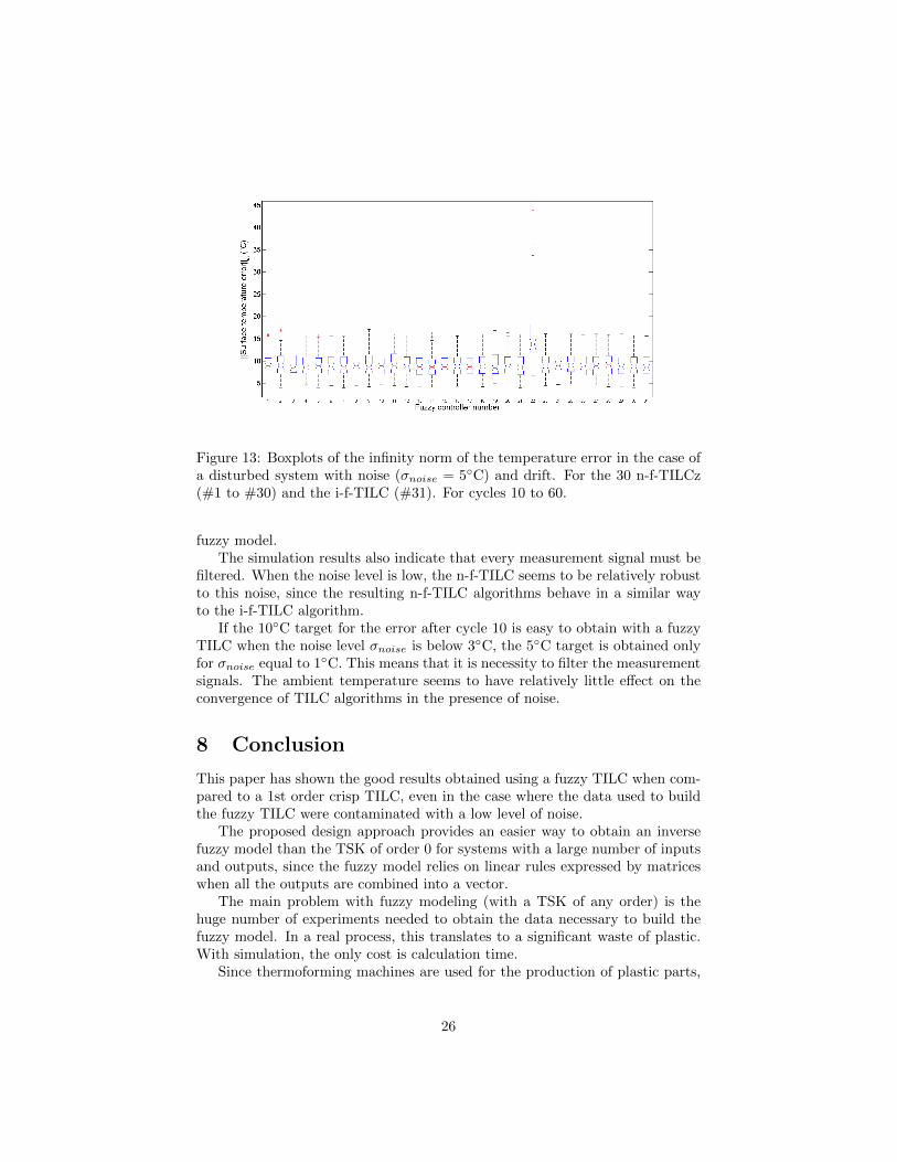
Figure 13: Boxplots of the infinity norm of the temperature error in the case ofa disturbed system with noise (σnoise = 5◦C) and drift. For the 30 n-f-TILCz(#1 to #30) and the i-f-TILC (#31). For cycles 10 to 60.

fuzzy model.The simulation results also indicate that every measurement signal must be

filtered. When the noise level is low, the n-f-TILC seems to be relatively robustto this noise, since the resulting n-f-TILC algorithms behave in a similar wayto the i-f-TILC algorithm.

If the 10◦C target for the error after cycle 10 is easy to obtain with a fuzzyTILC when the noise level σnoise is below 3◦C, the 5◦C target is obtained onlyfor σnoise equal to 1◦C. This means that it is necessity to filter the measurementsignals. The ambient temperature seems to have relatively little effect on theconvergence of TILC algorithms in the presence of noise.

8 Conclusion

This paper has shown the good results obtained using a fuzzy TILC when com-pared to a 1st order crisp TILC, even in the case where the data used to buildthe fuzzy TILC were contaminated with a low level of noise.

The proposed design approach provides an easier way to obtain an inversefuzzy model than the TSK of order 0 for systems with a large number of inputsand outputs, since the fuzzy model relies on linear rules expressed by matriceswhen all the outputs are combined into a vector.

The main problem with fuzzy modeling (with a TSK of any order) is thehuge number of experiments needed to obtain the data necessary to build thefuzzy model. In a real process, this translates to a significant waste of plastic.With simulation, the only cost is calculation time.

Since thermoforming machines are used for the production of plastic parts,

26

the data can be obtained from measurements performed on the actual produc-tion process. Building a fuzzy model from those measurements is work that wewill need to do in the future.

Another potential problem is the effect of noise when the data used to buildfuzzy model are obtained from measurements performed on a real process. Op-timistically, for the real thermoforming process, the noise level approximatelycorresponds to the simulations where σnoise = 1◦C. However, noise can becomean issue for other processes. Research is needed to analyze how noise can bereduced. A possible solution to this problem is to perform more than one mea-surement for each input tuple and to use the mean of those measurements asdata.

In future work, it will be interesting to analyze how the fuzzy model isobtained and inverted for the case where the number of inputs is not equal to thenumber of outputs. Moreover, since the simulation results are quite promising,we want to test the fuzzy TILC on an industrial thermoforming machine, aswe are convinced that this control can be used safely, without damaging themachine (by overheating).

9 Appendix [30]

This appendix is taken from [30].The nonlinear model of the thermoforming oven used in the simulations in

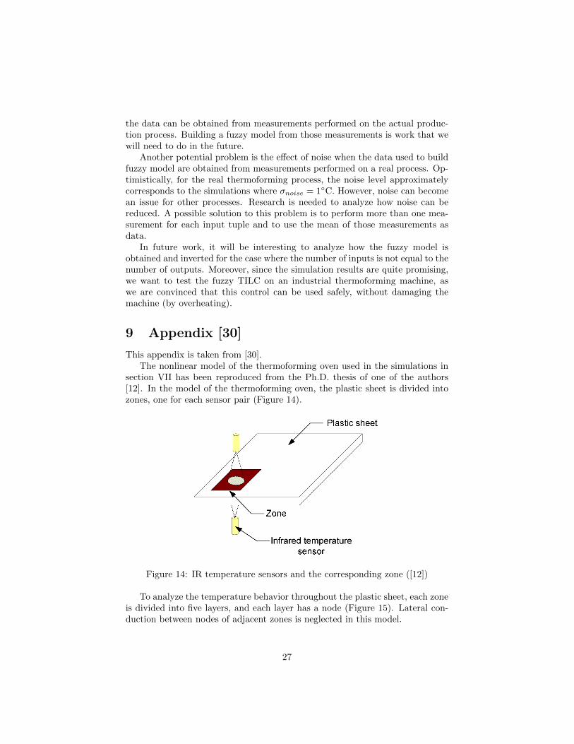
section VII has been reproduced from the Ph.D. thesis of one of the authors[12]. In the model of the thermoforming oven, the plastic sheet is divided intozones, one for each sensor pair (Figure 14).

Figure 14: IR temperature sensors and the corresponding zone ([12])

To analyze the temperature behavior throughout the plastic sheet, each zoneis divided into five layers, and each layer has a node (Figure 15). Lateral con-duction between nodes of adjacent zones is neglected in this model.

27

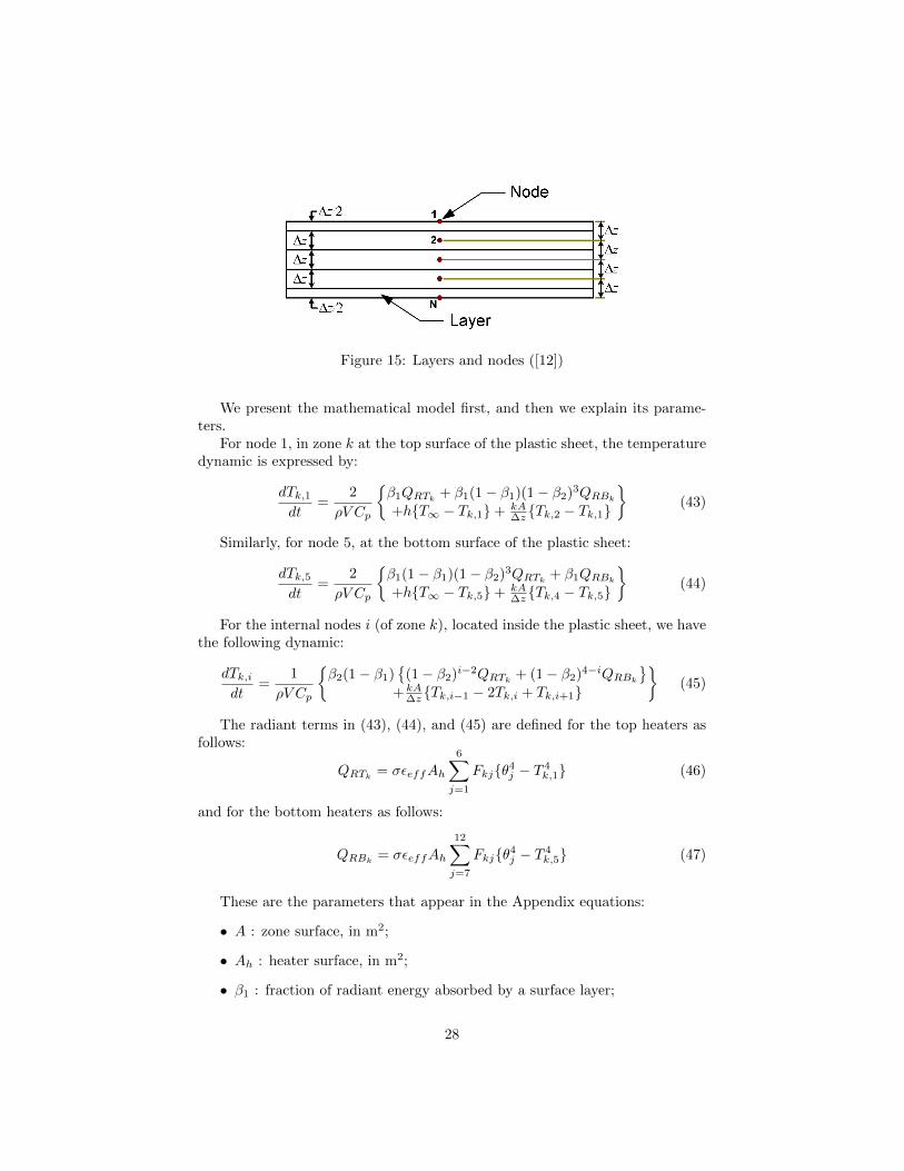
Figure 15: Layers and nodes ([12])

We present the mathematical model first, and then we explain its parame-ters.

For node 1, in zone k at the top surface of the plastic sheet, the temperaturedynamic is expressed by:

dTk,1dt

=2

ρV Cp

{β1QRTk

+ β1(1− β1)(1− β2)3QRBk

+h{T∞ − Tk,1}+ kA∆z{Tk,2 − Tk,1}

}(43)

Similarly, for node 5, at the bottom surface of the plastic sheet:

dTk,5dt

=2

ρV Cp

{β1(1− β1)(1− β2)3QRTk

+ β1QRBk

+h{T∞ − Tk,5}+ kA∆z{Tk,4 − Tk,5}

}(44)

For the internal nodes i (of zone k), located inside the plastic sheet, we havethe following dynamic:

dTk,idt

=1

ρV Cp

{β2(1− β1)

{(1− β2)i−2QRTk

+ (1− β2)4−iQRBk

}+ kA

∆z{Tk,i−1 − 2Tk,i + Tk,i+1}

}(45)

The radiant terms in (43), (44), and (45) are defined for the top heaters asfollows:

QRTk= σεeffAh

6∑j=1

Fkj{θ4j − T 4

k,1} (46)

and for the bottom heaters as follows:

QRBk= σεeffAh

12∑j=7

Fkj{θ4j − T 4

k,5} (47)

These are the parameters that appear in the Appendix equations:

• A : zone surface, in m2;

• Ah : heater surface, in m2;

• β1 : fraction of radiant energy absorbed by a surface layer;

28

• β2 : fraction of radiant energy absorbed by an internal layer;

• CP : specific heat of the plastic sheet, in J/(kg.K);

• εeff : effective emissivity;

• Fkj : view factor between heater j and sheet zone k;

• h : convection coefficient, in W/(m2.K);

• k : heat conduction constant, in W/(m.K);

• ρ : density of the plastic sheet, in kg/m3;

• T∞ : oven ambient temperature, in K;

• Tk,i : temperature of node i in zone k, in K;

• θj : temperature of heater j, in K;

• σ : Stefan Boltzmann constant equal to 5.669× 10−8 W/(m2.K4);

• ∆z : layer thickness, in meters;

• V : layer volume, in m3; (V = A∆z);

Additional details about this model can be found in chapter 2 in [12] orchapter 3 in [4].

References

[1] J. L. Throne and P. J. Mooney, “Thermoforming: Growth and evolution 1.”http://www.foamandform.com/technical-minutes/thermoforming/

thermoforming-growth-and-evolution-i, November 2002. Accessed:May 20, 2011.

[2] J. L. Throne, Technology of thermoforming. Hanser Publishers, 1996.

[3] J. Florian, Practical Thermoforming: Principles and Applications. MarcelDekker Inc., 1987.

[4] M. Ajersch, “Modeling and real-time control of sheet reheat phase in ther-moforming,” Master’s thesis, McGill University, 2004.

[5] M. M. I. Chy and B. Boulet, “A conjugate gradient method for the solutionof the inverse heating problem in thermoforming,” in 2010 IEEE IndustryApplications Society Annual Meeting, pp. 1–8, Oct 2010.

[6] P. Girard, R. di Raddo, V. Thomson, and B. Boulet, “Advanced in-cycleand cycle-to cycle on-line adaptive control for thermoforming of large ther-moplastic sheets,” in SAE Technical Paper, SAE International, 04 2005.

29

[7] F. M. Duarte and J. A. Covas, “Ir sheet heating in roll fed thermoforming:Part 1 - solving direct and inverse heating problems,” Plastics, Rubber andComposites, vol. 31, no. 7, pp. 307–317, 2002.

[8] Y. Chen, J.-X. Xu, and C. Wen, “A high-order terminal iterative learn-ing control scheme [rtp-cvd application],” in Proceedings of the 36th IEEEConference on Decision and Control, vol. 4, pp. 3771–3772, Dec 1997.

[9] Y. Chen, High-Order Iterative Learning Control: Convergence, Robustnessand Applications. PhD thesis, Nanyang Technological University: Singa-pore, 1997.

[10] K. L. Moore, Iterative Learning Control: An Expository Overview, pp. 151–214. Boston, MA: Birkhauser Boston, 1999.

[11] Y. Chen and C. Wen, eds., High-order terminal iterative learning controlwith an application to a rapid thermal process for chemical vapor deposition,pp. 95–104. London: Springer London, 1999.

[12] G. Gauthier, Terminal iterative learning for cycle-to-cycle control of in-dustrial processes. PhD thesis, Department of Electrical and ComputerEngineering. McGill University: Montreal, Canada, 2008.

[13] C. Zhang, H. Deng, and J. Baras, “Comparison of run-to-run control meth-ods in semiconductor manufacturing processes,” in AEC/APC SymposiumXII, Lake Tahoe, Nevada, 2000.

[14] J. Moyne, E. del Castillo, and A. Hurwitz, Run-to-Run Control in Semi-conductor Manufacturing. CRC Press, 2001.

[15] S. Adivikolanu and E. Zafiriou, “Robust run-to-run control for semiconduc-tor manufacturing: an internal model control approach,” in Proceedings ofthe 1998 American Control Conference, vol. 6, pp. 3687–3691, Jun 1998.

[16] E. Sachs, A. Hu, and A. Ingolfsson, “Run by run process control: com-bining spc and feedback control,” IEEE Transactions on SemiconductorManufacturing, vol. 8, pp. 26–43, Feb 1995.

[17] F. M. Duarte and J. A. Covas, “Ir sheet heating in roll fed thermoforming:Part 2 – factors influencing inverse heating solution,” Plastics, Rubber andComposites, vol. 32, no. 1, pp. 32–39, 2003.

[18] M. M. I. Chy and B. Boulet, “A new method for estimation and control oftemperature profile over a sheet in thermoforming process,” in 2010 IEEEIndustry Applications Society Annual Meeting, pp. 1–8, Oct 2010.

[19] M. Chy, B. Boulet, and G. Gauthier, Estimation and control of sheet tem-perature in thermoforming, ch. 9. Optimization of Polymer Processing,Nova Science Publishers, Inc, 2011.

30

[20] R. Boukezzoula, S. Galichet, and L. Foulloy, “Nonlinear internal model con-trol: application of inverse model based fuzzy control,” IEEE Transactionson Fuzzy Systems, vol. 11, pp. 814–829, Dec 2003.

[21] R. Boukezzoula, S. Galichet, and L. Foulloy, “Exact inversion of takagi-sugeno fuzzy models,” in Proceedings Joint 9th IFSA World Congressand 20th NAFIPS International Conference (Cat. No. 01TH8569), vol. 4,pp. 2108–2113, July 2001.

[22] S. A. Salman and G. S. Anavatti, “A novel inversion method for a fuzzymodel based controller,” in 2007 International Conference on Mechatronicsand Automation, pp. 100–104, Aug 2007.

[23] S. Galichet, R. Boukezzoula, and L. Foulloy, “Explicit analytical formu-lation and exact inversion of decomposable fuzzy systems with singletonconsequents,” Fuzzy Sets and Systems, vol. 146, no. 3, pp. 421 – 436, 2004.

[24] M. Fu, Z. Ding, G. Xia, and K. Fan, “Research on the fuzzy decouplingin the coordinated control system of nuclear power plant,” in 2008 IEEEInternational Conference on Automation and Logistics, pp. 405–410, Sept2008.

[25] A. Fortin, Analyse Numerique pour ingenieurs. Presses InternationalesPolytechnique, Montreal, 2001.

[26] M. Beauchemin-Turcotte, “Controle en fin de cycle par apprentissageiteratif via la logique floue appliquee au controle en temperature d’un fourde thermoformage,” Master’s thesis, Department of Automated Manufac-turing Engineering, Ecole de Technologie Superieure, 2010.

[27] B. Ogunnaike and W. Ray, Process Dynamics, Modeling, and Control. Ox-ford University Press, 1994.

[28] M. Morari and E. Zafiriou, Robust Process Control. Prentice Hall, 1989.

[29] R. Rakotomalada, “Comparaison de populations – tests nonparametriques.” http://eric.univ-lyon2.fr/~ricco/cours/cours/

Comp_Pop_Tests_Nonparametriques.pdf, August 2008. Accessed: March09, 2017.

[30] G. Gauthier and B. Boulet, “Terminal iterative learning control withinternal model control applied to the thermoforming reheat phase,” inAFRICON 2009, pp. 1–7, Sept 2009.

31