Université de Montréal

Avancées théoriques sur la représentationet l’optimisation des réseaux de neurones

parNicolas Le Roux

Département d’informatique et de recherche opérationnelleFaculté des arts et des sciences

Thèse présentée à la Faculté des études supérieuresen vue de l’obtention du grade de Philosophiæ Doctor (Ph.D.)

en informatique

Mars, 2008

c© Nicolas Le Roux, 2008.

Université de MontréalFaculté des études supérieures

Cette thèse intitulée:

Avancées théoriques sur la représentationet l’optimisation des réseaux de neurones

présentée par:

Nicolas Le Roux

a été évaluée par un jury composé des personnes suivantes:

Pierre L’Écuyer, président-rapporteurYoshua Bengio, directeur de recherchePascal Vincent, membre du juryYann LeCun, examinateur externeAlejandro Murua, représentant du doyen de la FES

Thèse acceptée le: . . . . . . . . . . . . . . . . . . . . . . . . . .

RÉSUMÉ

Les réseaux de neurones artificiels ont été abondamment utilisés dans la communauté

de l’apprentissage machine depuis les années 80. Bien qu’ils aient été étudiés pour la

première fois il y a cinquante ans par Rosenblatt [68], ils nefurent réellement populaires

qu’après l’apparition de la rétropropagation du gradient,en 1986 [71].

En 1989, il a été prouvé [44] qu’une classe spécifique de réseaux de neurones (les

réseaux de neurones à une couche cachée) était suffisamment puissante pour pouvoir

approximer presque n’importe quelle fonction avec une précision arbitraire : le théorème

d’approximation universelle. Toutefois, bien que ce théorème eût pour conséquence un

intérêt accru pour les réseaux de neurones, il semblerait qu’aucun effort n’ait été fait

pour profiter de cette propriété.

En outre, l’optimisation des réseaux de neurones à une couche cachée n’est pas

convexe. Cela a détourné une grande partie de la communauté vers d’autres algorithmes,

comme par exemple les machines à noyau (machines à vecteurs de support et régression

à noyau, entre autres).

La première partie de cette thèse présentera les concepts d’apprentissage machine

généraux nécessaires à la compréhension des algorithmes utilisés. La deuxième partie se

focalisera plus spécifiquement sur les méthodes à noyau et les réseaux de neurones.

La troisième partie de ce travail visera ensuite à étudier les limitations des machines

à noyaux et à comprendre les raisons pour lesquelles elles sont inadaptées à certains

problèmes que nous avons à traiter.

La quatrième partie présente une technique permettant d’optimiser les réseaux de

neurones à une couche cachée de manière convexe. Bien que cette technique s’avère

difficilement exploitable pour des problèmes de grande taille, une version approchée

permet d’obtenir une bonne solution dans un temps raisonnable.

La cinquième partie se concentre sur les réseaux de neuronesà une couche cachée

infinie. Cela leur permet théoriquement d’exploiter la propriété d’approximation univer-

selle et ainsi d’approcher facilement une plus grande classe de fonctions.

Toutefois, si ces deux variations sur les réseaux de neurones à une couche cachée

iv

leur confèrent des propriétés intéressantes, ces derniersne peuvent extraire plus que des

concepts de bas niveau. Les méthodes à noyau souffrant des mêmes limites, aucun de

ces deux types d’algorithmes ne peut appréhender des problèmes faisant appel à l’ap-

prentissage de concepts de haut niveau.

Récemment sont apparus les Deep Belief Networks [39] qui sont des réseaux de

neurones à plusieurs couches cachées entraînés de manière efficace. Cette profondeur

leur permet d’extraire des concepts de haut niveau et donc deréaliser des tâches hors

de portée des algorithmes conventionnels. La sixième partie étudie des propriétés de ces

réseaux profonds.

Les problèmes que l’on rencontre actuellement nécessitentnon seulement des algo-

rithmes capables d’extraire des concepts de haut niveau, mais également des méthodes

d’optimisation capables de traiter l’immense quantité de données parfois disponibles,

si possible en temps réel. La septième partie est donc la présentation d’une nouvelle

technique permettant une optimisation plus rapide.

Mots-clefs: méthodes à noyau, réseaux de neurones, convexité, descente de gradient,

réseaux profonds

ABSTRACT

Artificial Neural Networks have been widely used in the machine learning community

since the 1980’s. First studied more than fifty years ago [68], they became popular with

the apparition of gradient backpropagation in 1986 [71].

In 1989, Hornik et al. [44] proved that a specific class of neural networks (neural net-

works with one hidden layer) was powerful enough to approximate almost any function

with arbitrary precision: the universal approximation theorem. However, even though

this theorem resulted in increased interest for neural networks, few efforts have been

made to take advantage of this property.

Furthermore, the optimization of neural networks with one hidden layer is not con-

vex. This disenchanted a large part of the community which embraced other algorithms,

such as kernel machines (support vector machines and kernelregression, amongst oth-

ers).

The first part of this thesis will introduce the basics of machine learning needed for

the understanding of the algorithms which will be used. The second part will focus on

kernel machines and neural networks.

The third part will study the limits of kernel machines and try to understand the rea-

sons of their inability to handle some of the more challenging problems we are interested

in.

The fourth part introduces a technique allowing a convex optimization of the neural

networks with one hidden layer. Even though this technique is impractical for medium

and large scale problems, its approximation leads to good solutions achieved in reason-

able times.

The fifth part focuses on neural networks with an infinite hidden layer. This allows

them to exploit the universal approximation property and therefore to easily model a

larger class of functions than standard neural networks.

However, though these two variations on neural networks with one hidden layer show

interesting properties, they cannot extract high level concepts any better. Kernel ma-

chines suffering from the same curse, none of these familiesof algorithms can handle

vi

problems requiring the learning of high level concepts.

Introduced in 2006, Deep Belief Networks [39] are neural networks with many hid-

den layers trained in a greedy way. Their depth allows them toextract high level concepts

and thus to perform tasks out of the reach of standard algorithms. The sixth part of this

thesis will present some of the properties of these networks.

Problems one has to face today not only require powerful representations, but also

efficient optimization techniques able to handle the enormous quantity of data available,

in real time if possible. The seventh part is therefore a presentation of a new and efficient

online second order gradient descent method.

Keywords: kernel methods, neural networks, convexity, gradient descent, deep net-

works

TABLE DES MATIÈRES

RÉSUMÉ . . . . . . . . . . . . . . . . . . . . . . . . . . . . . . . . . . . . . iii

ABSTRACT . . . . . . . . . . . . . . . . . . . . . . . . . . . . . . . . . . . . v

TABLE DES MATIÈRES . . . . . . . . . . . . . . . . . . . . . . . . . . . . vii

LISTE DES TABLEAUX . . . . . . . . . . . . . . . . . . . . . . . . . . . . . xiii

LISTE DES FIGURES . . . . . . . . . . . . . . . . . . . . . . . . . . . . . . xiv

REMERCIEMENTS . . . . . . . . . . . . . . . . . . . . . . . . . . . . . . . xvii

AVANT-PROPOS . . . . . . . . . . . . . . . . . . . . . . . . . . . . . . . . . xviii

CHAPITRE 1 : INTRODUCTION À L’APPRENTISSAGE MACHINE . . 1

1.1 L’apprentissage chez les humains . . . . . . . . . . . . . . . . . . .. . 1

1.2 L’apprentissage machine . . . . . . . . . . . . . . . . . . . . . . . . . 2

1.2.1 Qu’est-ce qu’un bon apprentissage ? . . . . . . . . . . . . . . .3

1.2.2 Et l’apprentissage par règles ? . . . . . . . . . . . . . . . . . . 4

1.3 Différents types d’apprentissage . . . . . . . . . . . . . . . . . .. . . 5

1.3.1 Apprentissage supervisé . . . . . . . . . . . . . . . . . . . . . 5

1.3.2 Apprentissage non supervisé . . . . . . . . . . . . . . . . . . . 7

1.3.3 Apprentissage semi-supervisé . . . . . . . . . . . . . . . . . . 9

1.4 Entraînement, test et coûts . . . . . . . . . . . . . . . . . . . . . . . .10

1.4.1 Algorithmes et paramètres . . . . . . . . . . . . . . . . . . . . 10

1.4.2 Entraînement et test . . . . . . . . . . . . . . . . . . . . . . . . 11

1.4.3 Coûts et erreurs . . . . . . . . . . . . . . . . . . . . . . . . . . 12

1.5 Régularisation . . . . . . . . . . . . . . . . . . . . . . . . . . . . . . . 14

1.5.1 Limitation du nombres de paramètres . . . . . . . . . . . . . . 17

1.5.2 Pénalisation des poids (« weight decay») . . . . . . . . . . . . 17

viii

1.5.3 Discussion . . . . . . . . . . . . . . . . . . . . . . . . . . . . 18

1.6 Théorème de Bayes . . . . . . . . . . . . . . . . . . . . . . . . . . . . 19

1.6.1 Maximum A Posteriori . . . . . . . . . . . . . . . . . . . . . . 21

1.6.2 Apprentissage bayésien . . . . . . . . . . . . . . . . . . . . . . 22

1.6.3 Interprétation bayésienne du coût . . . . . . . . . . . . . . . .23

CHAPITRE 2 : MÉTHODES À NOYAU ET RÉSEAUX DE NEURONES 27

2.1 Les méthodes à noyau . . . . . . . . . . . . . . . . . . . . . . . . . . . 27

2.1.1 Principe des méthodes à noyau . . . . . . . . . . . . . . . . . . 27

2.1.2 Espace de Hilbert à noyau reproduisant . . . . . . . . . . . . .28

2.1.3 Théorème du représentant . . . . . . . . . . . . . . . . . . . . 29

2.1.4 Processus gaussiens . . . . . . . . . . . . . . . . . . . . . . . 30

2.2 Réseaux de neurones . . . . . . . . . . . . . . . . . . . . . . . . . . . 30

2.2.1 Les réseaux de neurones à propagation avant . . . . . . . . .. 32

2.2.2 Fonction de transfert . . . . . . . . . . . . . . . . . . . . . . . 33

2.2.3 Terminologie . . . . . . . . . . . . . . . . . . . . . . . . . . . 34

2.2.4 Loi a priori sur les poids et a priori sur les fonctions .. . . . . . 36

2.2.5 Liens entre les machines à noyau et les réseaux de neurones . . 37

2.3 Descente de gradient . . . . . . . . . . . . . . . . . . . . . . . . . . . 38

CHAPITRE 3 : PRÉSENTATION DU PREMIER ARTICLE . . . . . . . 40

3.1 Détails de l’article . . . . . . . . . . . . . . . . . . . . . . . . . . . . . 40

3.2 Contexte . . . . . . . . . . . . . . . . . . . . . . . . . . . . . . . . . . 40

3.3 Commentaires . . . . . . . . . . . . . . . . . . . . . . . . . . . . . . . 41

CHAPITRE 4 : THE CURSE OF HIGHLY VARIABLE FUNCTIONS FOR

LOCAL KERNEL MACHINES . . . . . . . . . . . . . . 42

4.1 Abstract . . . . . . . . . . . . . . . . . . . . . . . . . . . . . . . . . . 42

4.2 Introduction . . . . . . . . . . . . . . . . . . . . . . . . . . . . . . . . 42

4.3 The Curse of Dimensionality for Classical Non-Parametric Models . . . 45

4.3.1 The Bias-Variance Dilemma . . . . . . . . . . . . . . . . . . . 45

ix

4.3.2 Dimensionality and Rate of Convergence . . . . . . . . . . . .46

4.4 Summary of the results . . . . . . . . . . . . . . . . . . . . . . . . . . 48

4.5 Minimum Number of Bases Required for Complex Functions .. . . . . 49

4.5.1 Limitations of Learning with Gaussians . . . . . . . . . . . .. 49

4.5.2 Learning thed-Bits Parity Function . . . . . . . . . . . . . . . 51

4.6 When a Test Example is Far from Training Examples . . . . . . .. . . 55

4.7 Locality of the Estimator and its Tangent . . . . . . . . . . . . .. . . . 57

4.7.1 Geometry of Tangent Planes . . . . . . . . . . . . . . . . . . . 59

4.7.2 Geometry of Decision Surfaces . . . . . . . . . . . . . . . . . 59

4.8 The Curse of Dimensionality for Local Non-Parametric Semi-Supervised

Learning . . . . . . . . . . . . . . . . . . . . . . . . . . . . . . . . . . 61

4.9 General Curse of Dimensionality Argument . . . . . . . . . . . .. . . 63

4.10 Conclusion . . . . . . . . . . . . . . . . . . . . . . . . . . . . . . . . 66

CHAPITRE 5 : PRÉSENTATION DU DEUXIÈME ARTICLE . . . . . . 67

5.1 Détails de l’article . . . . . . . . . . . . . . . . . . . . . . . . . . . . . 67

5.2 Contexte . . . . . . . . . . . . . . . . . . . . . . . . . . . . . . . . . . 67

5.2.1 Convexité . . . . . . . . . . . . . . . . . . . . . . . . . . . . . 68

5.2.2 Fonction de coût et optimisation . . . . . . . . . . . . . . . . . 68

5.3 Commentaires . . . . . . . . . . . . . . . . . . . . . . . . . . . . . . . 69

CHAPITRE 6 : CONVEX NEURAL NETWORKS . . . . . . . . . . . . . 70

6.1 Abstract . . . . . . . . . . . . . . . . . . . . . . . . . . . . . . . . . . 70

6.2 Introduction . . . . . . . . . . . . . . . . . . . . . . . . . . . . . . . . 70

6.3 Core Ideas . . . . . . . . . . . . . . . . . . . . . . . . . . . . . . . . . 72

6.4 Finite Number of Hidden Neurons . . . . . . . . . . . . . . . . . . . . 75

6.5 Incremental Convex NN Algorithm . . . . . . . . . . . . . . . . . . . .76

6.6 Conclusion . . . . . . . . . . . . . . . . . . . . . . . . . . . . . . . . 82

CHAPITRE 7 : PRÉSENTATION DU TROISIÈME ARTICLE . . . . . . 84

7.1 Détails de l’article . . . . . . . . . . . . . . . . . . . . . . . . . . . . . 84

x

7.2 Contexte . . . . . . . . . . . . . . . . . . . . . . . . . . . . . . . . . . 84

7.3 Commentaires . . . . . . . . . . . . . . . . . . . . . . . . . . . . . . . 84

CHAPITRE 8 : CONTINUOUS NEURAL NETWORKS . . . . . . . . . . 86

8.1 Abstract . . . . . . . . . . . . . . . . . . . . . . . . . . . . . . . . . . 86

8.2 Introduction . . . . . . . . . . . . . . . . . . . . . . . . . . . . . . . . 86

8.3 Affine neural networks . . . . . . . . . . . . . . . . . . . . . . . . . . 88

8.3.1 Core idea . . . . . . . . . . . . . . . . . . . . . . . . . . . . . 88

8.3.2 Approximating an Integral . . . . . . . . . . . . . . . . . . . . 89

8.3.3 Piecewise Affine Parametrization . . . . . . . . . . . . . . . . 90

8.3.4 Extension to multiple output neurons . . . . . . . . . . . . . .91

8.3.5 Piecewise affine versus piecewise constant . . . . . . . . .. . 91

8.3.6 Implied prior distribution . . . . . . . . . . . . . . . . . . . . . 94

8.3.7 Experiments . . . . . . . . . . . . . . . . . . . . . . . . . . . 97

8.4 Non-Parametric Continous Neural Networks . . . . . . . . . . .. . . . 100

8.4.1 L1-norm Output Weights Regularization . . . . . . . . . . . . . 101

8.4.2 L2-norm Output Weights Regularization . . . . . . . . . . . . . 101

8.4.3 Kernel wheng is thesign Function . . . . . . . . . . . . . . . 102

8.4.4 Conclusions, Discussion, and Future Work . . . . . . . . . .. 106

CHAPITRE 9 : PRÉSENTATION DU QUATRIÈME ARTICLE . . . . . . 107

9.1 Détails de l’article . . . . . . . . . . . . . . . . . . . . . . . . . . . . . 107

9.2 Contexte . . . . . . . . . . . . . . . . . . . . . . . . . . . . . . . . . . 107

9.2.1 Approches précédentes . . . . . . . . . . . . . . . . . . . . . . 107

9.3 Commentaires . . . . . . . . . . . . . . . . . . . . . . . . . . . . . . . 109

CHAPITRE 10 : REPRESENTATIONAL POWER OF RESTRICTED BOLTZ-

MANN MACHINES AND DEEP BELIEF NETWORKS . 111

10.1 Abstract . . . . . . . . . . . . . . . . . . . . . . . . . . . . . . . . . . 111

10.2 Introduction . . . . . . . . . . . . . . . . . . . . . . . . . . . . . . . . 111

10.2.1 Background on RBMs . . . . . . . . . . . . . . . . . . . . . . 113

xi

10.3 RBMs are Universal Approximators . . . . . . . . . . . . . . . . . .. 114

10.3.1 Better Model with Increasing Number of Units . . . . . . .. . 115

10.3.2 A Huge Model can Represent Any Distribution . . . . . . . .. 117

10.4 Representational power of Deep Belief Networks . . . . . .. . . . . . 118

10.4.1 Background on Deep Belief Networks . . . . . . . . . . . . . . 118

10.4.2 Trying to Anticipate a High-Capacity Top Layer . . . . .. . . 119

10.4.3 Open Questions on DBN Representational Power . . . . . .. . 123

10.5 Conclusions . . . . . . . . . . . . . . . . . . . . . . . . . . . . . . . . 125

10.6 Appendix . . . . . . . . . . . . . . . . . . . . . . . . . . . . . . . . . 126

10.6.1 Proof of Lemma 10.3.1 . . . . . . . . . . . . . . . . . . . . . . 126

10.6.2 Proof of theorem 10.3.3 . . . . . . . . . . . . . . . . . . . . . 127

10.6.3 Proof of theorem 10.3.4 . . . . . . . . . . . . . . . . . . . . . 130

CHAPITRE 11 : PRÉSENTATION DU CINQUIÈME ARTICLE . . . . . . 133

11.1 Détails de l’article . . . . . . . . . . . . . . . . . . . . . . . . . . . . .133

11.2 Contexte . . . . . . . . . . . . . . . . . . . . . . . . . . . . . . . . . . 133

11.3 Bilan . . . . . . . . . . . . . . . . . . . . . . . . . . . . . . . . . . . . 133

CHAPITRE 12 : TOPMOUMOUTE ONLINE NATURAL GRADIENT AL-

GORITHM . . . . . . . . . . . . . . . . . . . . . . . . . . 135

12.1 Abstract . . . . . . . . . . . . . . . . . . . . . . . . . . . . . . . . . . 135

12.2 Natural gradient . . . . . . . . . . . . . . . . . . . . . . . . . . . . . . 136

12.3 A new justification for natural gradient . . . . . . . . . . . . .. . . . . 137

12.3.1 Bayesian setting . . . . . . . . . . . . . . . . . . . . . . . . . 138

12.3.2 Frequentist setting . . . . . . . . . . . . . . . . . . . . . . . . 139

12.4 Online natural gradient . . . . . . . . . . . . . . . . . . . . . . . . . .140

12.4.1 Low complexity natural gradient implementations . .. . . . . 140

12.4.2 TONGA . . . . . . . . . . . . . . . . . . . . . . . . . . . . . . 141

12.5 Block-diagonal online natural gradient for neural networks . . . . . . . 144

12.6 Experiments . . . . . . . . . . . . . . . . . . . . . . . . . . . . . . . . 146

12.6.1 MNIST dataset . . . . . . . . . . . . . . . . . . . . . . . . . . 147

xii

12.6.2 Rectangles problem . . . . . . . . . . . . . . . . . . . . . . . . 148

12.7 Discussion . . . . . . . . . . . . . . . . . . . . . . . . . . . . . . . . . 148

CHAPITRE 13 : CONCLUSION . . . . . . . . . . . . . . . . . . . . . . . 151

13.1 Synthèse des articles . . . . . . . . . . . . . . . . . . . . . . . . . . . 151

13.1.1 The Curse of Highly Variable Functions for Local Kernel Machines151

13.1.2 Convex Neural Networks . . . . . . . . . . . . . . . . . . . . . 152

13.1.3 Continuous Neural Networks . . . . . . . . . . . . . . . . . . . 153

13.1.4 Representational Power of Restricted Boltzmann Machines and

Deep Belief Networks . . . . . . . . . . . . . . . . . . . . . . 153

13.1.5 Topmoumoute Online Natural Gradient Algorithm . . . .. . . 153

13.2 Conclusion . . . . . . . . . . . . . . . . . . . . . . . . . . . . . . . . 153

BIBLIOGRAPHIE . . . . . . . . . . . . . . . . . . . . . . . . . . . . . . . . 158

LISTE DES TABLEAUX

8.1 sign kernelvsGaussian kernel on USPS dataset, with different Gaussian

widthsσ and weight decaysλ. . . . . . . . . . . . . . . . . . . . . . . 105

LISTE DES FIGURES

1.1 Exemple de problème de classification : que représententces deux images ? 6

1.2 Si un canon tire des boulets sur un champ selon une distribution fixe mais

inconnue et qu’on connaît les points d’impact des 500 premiers boulets,

peut-on estimer cette distribution ? . . . . . . . . . . . . . . . . . . .. 7

1.3 Exemple de solutions de complexités différentes pour deux problèmes

d’apprentissage : en haut, de l’estimation de densité et en bas, de la ré-

gression.Gauche : données d’entraînement.Milieu : solution simple

(régularisée).Droite : solution compliquée (non régularisée). . . . . . . 16

2.1 Architecture d’un réseau de neurones à propagation avant à une couche

cachée et sans fonction de sortie. . . . . . . . . . . . . . . . . . . . . . 33

2.2 En haut à gauche :σ = 1. En haut à droite :σ = 5. En bas à gauche :

σ = 20. En bas à droite :σ = 100. . . . . . . . . . . . . . . . . . . . . 38

4.1 The dotted line crosses the decision surface 19 times : one thus needs at

least 10 Gaussians to learn it with an affine combination of Gaussians

with same width. . . . . . . . . . . . . . . . . . . . . . . . . . . . . . 50

4.2 Plot ofze−z2. . . . . . . . . . . . . . . . . . . . . . . . . . . . . . . . 60

8.1 Functions generated by an ordinary neural network (top)and an affine

neural network (bottom) with 2 hidden units andσu = 5 (left), σu = 20

(mid) andσu = 100 (right) (σa = σu andσb = wv = 1). . . . . . . . . . 95

8.2 Functions generated by an ordinary neural network (top)and an affine

neural network (bottom) with 10 hidden units andσu = 5 (left), σu = 20

(mid) andσu = 100 (right) (σa = σu andσb = wv = 1). . . . . . . . . . 96

8.3 Functions generated by an ordinary neural network (up) and an affine

neural network (down) with 10000 hidden units andσu = 5 (left), σu =

20 (mid) andσu = 100 (right) (σa = σu andσb = wv = 1). . . . . . . . 96

xv

8.4 Training curves for both algorithms on the USPS dataset with 7 hidden

units. . . . . . . . . . . . . . . . . . . . . . . . . . . . . . . . . . . . 98

8.5 Training curves for both algorithms on the LETTERS dataset with 50

and 100 hidden units. . . . . . . . . . . . . . . . . . . . . . . . . . . . 99

8.6 Training curves for both algorithms on random datasets.Left : 196 ran-

dom inputs and 5 random targets, using networks with 10 hidden units

and the MSE. Right : Inputs of the USPS dataset and 1 random label,

using networks with 7 hidden units and the NLL. . . . . . . . . . . . .100

8.7 Two functions drawn from the Gaussian process associated to the above

kernel function. . . . . . . . . . . . . . . . . . . . . . . . . . . . . . . 105

10.1 Greedy learning of an RBM. After each RBM has been trained, the

weights are frozen and a new layer is added. The new layer is trained

as an RBM. . . . . . . . . . . . . . . . . . . . . . . . . . . . . . . . . 119

10.2 KL divergence w.r.t. number epochs after adding the 2ndlevel RBM,

between empirical distributionp0 (either training or test set) and (top

curves) DBN trained greedily with contrastive divergence at each layer,

or (bottom curves) DBN trained greedily withKL(p0||p1) on the 1st

layer, and contrastive divergence on the 2nd. . . . . . . . . . . . .. . . 124

12.1 Absolute correlation between the standard stochasticgradients after one

epoch in a neural network with 16 input units, 50 hidden unitsand 26

output units when following stochastic gradient directions (left) and na-

tural gradient directions (center and right). . . . . . . . . . . .. . . . . 145

12.2 Quality of the approximationC of the covarianceC depending on the

number of eigenvectors kept (k), in terms of the ratio of Frobenius norms‖C−C‖2

F

‖C‖2F

, for different types of approximationsC (full matrix or block

diagonal) . . . . . . . . . . . . . . . . . . . . . . . . . . . . . . . . . 146

xvi

12.3 Comparison between stochastic gradient and TONGA on the MNIST da-

taset (50000 training examples), in terms of training and test classifica-

tion error and Negative Log-Likelihood (NLL). The mean and standard

error have been computed using 9 different initializations. . . . . . . . . 147

12.4 Comparison between stochastic gradient descent and TONGA w.r.t. NLL

and classification error, on training and validation sets for the rectangles

problem (900,000 training examples). . . . . . . . . . . . . . . . . . .150

REMERCIEMENTS

Je tiens tout d’abord à remercier Yoshua Bengio pour m’avoiraccueilli dans son

laboratoire, guidé et conseillé tout au long de ces années. Son soutien indéfectible, ses

encouragements et la confiance qu’il a placée en moi m’ont donné l’assurance et le

courage nécessaire pour poursuivre dans cette voie.

Je tiens aussi à remercier Pierre-Antoine Manzagol pour m’avoir encouragé à re-

mettre en question ce que je croyais savoir, pour les nombreuses discussions qu’on a

eues et pour avoir aidé mon insertion à Montréal.

Je remercie encore tous ceux du LISA qui m’ont stimulé intellectuellement, sont

venus m’aider quand j’en avais besoin et m’ont forcé à écrirecette thèse.

Enfin, je tiens à remercier Muriel pour avoir supporté mes doutes, ma fatigue et mes

cours improvisés sur les réseaux de neurones pendant les repas.

AVANT-PROPOS

« Il avait appris sans effort l’anglais, le français, le portugais, le latin. Je

soupçonne cependant qu’il n’était pas très capable de penser. Penser c’est

oublier des différences, c’est généraliser, abstraire. Dans le monde surchargé

de Funes, il n’y avait que des détails, presque immédiats.»

Jorge Luis Borges, inFunes ou la mémoire

xix

À ma famille, pour son soutien indéfectible.. . .

CHAPITRE 1

INTRODUCTION À L’APPRENTISSAGE MACHINE

1.1 L’apprentissage chez les humains

Les humains apprennent de deux manières différentes :

– par règles, c’est-à-dire qu’un élément extérieur (livre,professeur, parent, ...) définit

un concept et ce qui le caractérise

– par l’expérience, c’est-à-dire que l’observation du monde qui les entoure leur per-

met d’affiner leur définition d’un concept1.

Il est intéressant de remarquer que des concepts qui nous apparaissent élémentaires,

comme de savoir ce qu’est un chien, reposent bien plus sur l’expérience que sur des

règles définies. Le Trésor de la Langue Française informatisé (http://atilf.atilf.

fr), par exemple, définit le chien comme un« mammifère carnivore très anciennement

domestiqué, dressé à la garde des maisons et des troupeaux, àla chasse ou bien élevé

pour l’agrément». Bien qu’exacte, cette définition nous est inutile lorsqu’il s’agit de

différencier un chien d’un chat dans la rue.

Il nous est d’ailleurs quasiment impossible de définir précisément les critères défi-

nissant le concept« chien» que nous utilisons. Pour s’en convaincre, voyons les trois

exemples suivants :

– un chien à qui on a enfilé un costume d’autruche est-il toujours un chien ?

– un chien à qui on a coupé les cordes vocales et transformé chirurgicalement pour

qu’il ressemble à une autruche est-il toujours un chien ?

– un chien qu’on a modifié génétiquement pour qu’il ressembleà une autruche, qu’il

puisse se reproduire avec les autruches mais pas avec les chiens est-il toujours un

chien ?

Si la réponse à la première de ces questions nous apparaît évidente, il est plus malaisé

de répondre aux deux dernières. Nous avons donc, en tant qu’humains, développé une

1les animaux n’apprennent que par l’expérience et par imitation, méthode qui peut être assimilée à del’expérience.

2

conception très précise de ce qu’est un chien pour faire faceaux situations de la vie

courante. Les exemples présentés ci-dessus n’étant pas desexemples courants (sauf celui

du déguisement dont on connaît bien les conséquences), notre définition est tout à coup

prise en défaut.

Cette conception, personne ne nous l’a apprise. La premièrefois que nous avons vu

un chien, un élément extérieur (livre, professeur, parent,...) nous l’a nommé comme tel

puis, découvrant le monde, nous avons vu de nombreux chiens jusqu’à en peaufiner une

définition qui est celle que chacun de nous a. Il est d’ailleurs vraisemblable que, dans

différentes parties du monde (et même peut-être chez chaquehumain), la représentation

mentale d’un chien diffère, quand bien même la définition dans les dictionnaires serait la

même.C’est donc bien la succession d’exemples qui nous ont été présentés qui nous

a permis de« définir » très précisément ce qu’était un chien.

De même, un enfant arrivera à créer des nouvelles phrases sans que les notions

de sujet, verbe ou complément lui aient été apprises. C’est donc la simple succession

d’exemples (les phrases qui ont été prononcées devant lui) qui a amené cette compré-

hension de la structure syntaxique d’une phrase.

1.2 L’apprentissage machine

L’apprentissage machine est un domaine à la jonction des statistiques et de l’intel-

ligence artificielle qui a pour but de créer des algorithmes capables d’effectuer cette

extraction de concepts à partir d’exemples.

Un algorithme d’apprentissage est une fonction mathématiqueA qui prend comme

argument un ensemble d’exemplesD et qui renvoie une fonctionf , ou, plus formelle-

ment :

A : (X × Y)N → YX (1.1)

D → A(D) = f

oùX est l’espace des entrées etY l’espace des sorties. Dans l’exemple de la section pré-

3

cédente,D représenterait l’ensemble des informations acquises au cours de notre vie (ce

qu’on a vu ou entendu, par exemple) etf serait la fonction déterminant si un objet est un

chien ou pas.A, au contraire, représente notre patrimoine génétique qui détermine notre

réaction à la présentation d’exemples et le spectre des fonctions engendrées possibles.

Les règles qui nous ont été apprises requièrent l’extraction de concepts (la transforma-

tion de ces règles en données sensorielles) pour les appliquer au monde réel. En ce sens,

elles sont modélisées parD. Toutefois, elles peuvent parfois se présenter sous formesde

vérités universelles qui contraindront la fonction finale,quels que soient les exemples

vus par la suite, et doivent alors être modélisées parA.

1.2.1 Qu’est-ce qu’un bon apprentissage ?

On associe souvent un bon apprentissage avec une bonne mémoire. Cela est valide

lorsque la tâche à effectuer suit des règles bien établies etque ces règles nous sont don-

nées. En revanche, lorsqu’il s’agit de généraliser une règle à partir d’exemples, cela

devient incongru. Si un humain n’a vu que dix chiens dans sa vie, doit-il en conclure que

seuls ceux-là sont des chiens et qu’aucun autre élément du monde ne peut être un chien ?

Que dire de ces mêmes chiens vus sous un angle différent ? Un ordinateur est excellent

pour apprendre par cœur, c’est-à-dire pour réaliser la tâche demandée sur les exemples

dont il s’est servi pour apprendre. En revanche, il est bien plus complexe de développer

un algorithme capable de généraliser la tâche apprise à de nouveaux exemples.

La phase d’apprentissage d’un algorithme s’appelle aussi la phase d’entraînement.

Lors de cette phase, l’algorithme se voit présenter des exemples sur lesquels il doit réali-

ser la tâche demandée. Ainsi, on lui présentera par exemple des images de chiens et d’au-

truches pour ensuite lui demander de faire la distinction entre ces deux types d’animaux.

Lors de la phase detest, l’algorithme doit réaliser la tâche demandée sur de nouveaux

exemples. S’il lui est présenté un chien d’une race jamais vue auparavant, saura-t-il dé-

terminer correctement sa nature ?

L’idée sous-jacente de la phase d’apprentissage est que, s’il arrive à effectuer cor-

rectement la tâche demandée sur les exemples qui lui sont présentés (les exemples

d’apprentissageou exemples d’entraînement), il en a extrait les concepts importants

4

et sera à même de l’effectuer sur de nouveaux exemples (les exemples detest). En effet,

ce qui nous intéresse réellement est la capacité de généralisation d’un algorithme, afin

qu’il puisse être utilisé dans des environnements nouveaux. Malheureusement, il arrive

parfois qu’un algorithme ne fasse aucune erreur sur les exemples d’apprentissage sans

pour autant en avoir extrait aucun concept. Il suffit pour s’en rendre compte d’imaginer

un algorithme se contentant d’apprendre par cœur. Si sa performance sur les exemples

d’entraînement sera parfaite, rien ne nous permet d’affirmer qu’il sera en mesure d’utili-

ser ses connaissances sur de nouveaux exemples. Il est donc extrêmement important de

garder constamment à l’esprit cette différence entre performance en entraînement et en

généralisation. Toute la subtilité de l’apprentissage statistique repose sur ce paradigme :

créer des algorithmes ayant une bonne capacité de généralisation alors même que nous

n’avons à notre disposition qu’un nombre limité d’exemplesd’entraînement.

1.2.2 Et l’apprentissage par règles ?

Une question subsiste : puisque l’apprentissage humain se fait par des règles et par

l’expérience, peut-on également utiliser des règles pour l’apprentissage machine ?

Il est en effet tout à fait possible d’introduire des règles dans l’apprentissage machine.

Dans ce cas, le concepteur de l’algorithme joue le rôle du professeur et introduit ses

connaissancesa priori en influant sur la structure de l’algorithme. Si cette approche

est valide et efficace lorsqu’on veut résoudre un problème enparticulier, elle est plus

problématique si notre but est de créer une vraie intelligence sans supervision, et ce pour

plusieurs raisons. Tout d’abord, le nombre total de règles àdéfinir augmente linéairement

avec le nombre de tâches à réaliser, ce qui devient vite irréalisable dès lors qu’on souhaite

un algorithme (relativement) général. En outre, les règlessont des principes intangibles,

dont la portée est fréquemment limitée par des exceptions. Ces dernières rendent encore

plus ardue l’exhaustivité et la cohérence globale de cet ensemble. Enfin, l’évolution de

l’humain a été majoritairement guidée par son apprentissage, que celui-là ait été acquis

ou transmis par la génération précédente. Il semble donc raisonnable d’espérer parvenir

au même résultat en utilisant les mêmes moyens.

Si les deux visions coexistent au sein de la communauté, mon souhait étant de dé-

5

couvrir l’intelligence la plus générale possible, je limiterai au maximum la quantité d’in-

formations manuellement introduite dans mes algorithmes.

1.3 Différents types d’apprentissage

Ce travail portera sur trois catégories de tâches qu’on peutaccomplir avec des algo-

rithmes d’apprentissage machine :

– l’apprentissage supervisé

– l’apprentissage non supervisé

– l’apprentissage semi-supervisé

Une présentation de ces trois types d’apprentissage peut-être trouvée dans [20, p.3].

Je ne parlerai volontairement pas de l’apprentissage par renforcement, domaine à la fois

plus général et plus difficile, mais dont les trois tâches précitées sont des éléments consti-

tutifs.

1.3.1 Apprentissage supervisé

Dans l’apprentissage supervisé, les données fournies sontdes paires : uneentréeet

uneétiquette. On parle alors d’entrées étiquetées. L’entrée est un élément associé à

une valeur ou à une classe et l’étiquette est la valeur ou la classe associée. Le but de

l’apprentissage est d’inférer la valeur de l’étiquette étant donnée la valeur de l’entrée.

On peut distinguer deux grands types d’apprentissage supervisé : laclassificationet

la régression.

1.3.1.1 Classification

Lorqu’on fait de la classification, l’entrée est l’instanced’une classe et l’étiquette est

la classe correspondante. En reconnaissance de caractères, par exemple, l’entrée serait

une suite de pixels représentant une lettre et la classe serait la lettre représentée (ou son

index).

La classification consiste donc à apprendre une fonctionfclass deRd dansN qui as-

socie à un vecteur sa classe. Dans certains cas, on pourra vouloir que la fonctionfclass

6

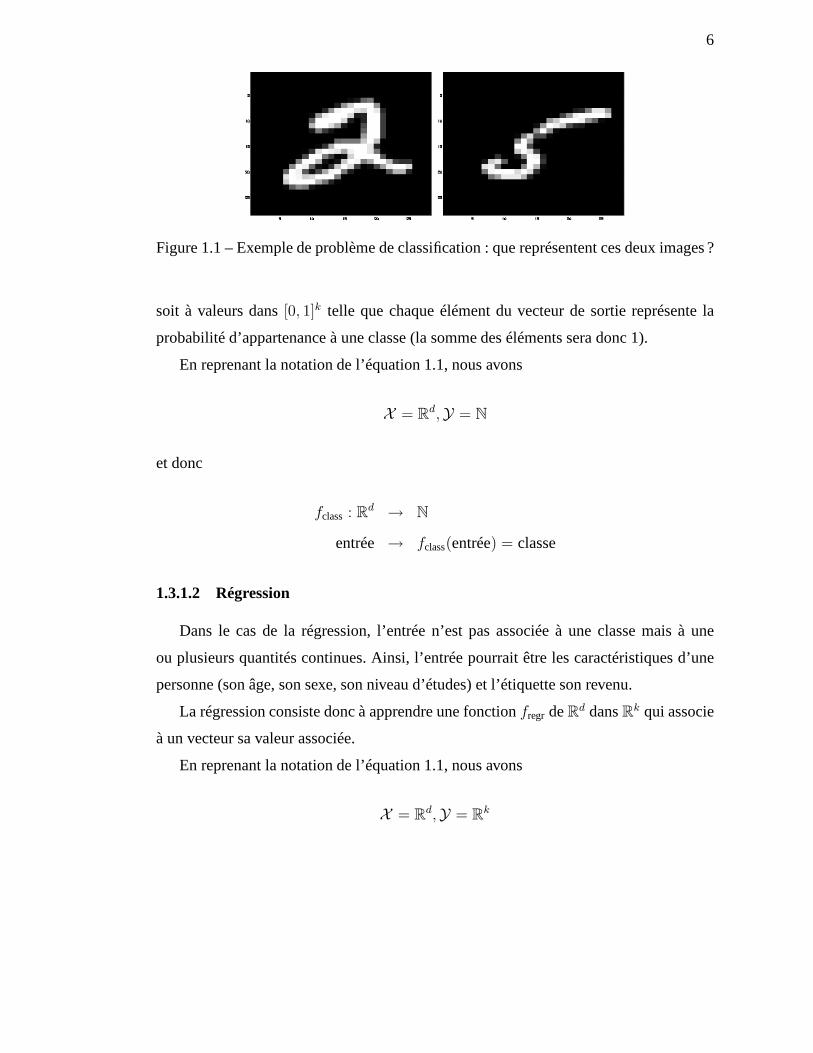
Figure 1.1 – Exemple de problème de classification : que représentent ces deux images ?

soit à valeurs dans[0, 1]k telle que chaque élément du vecteur de sortie représente la

probabilité d’appartenance à une classe (la somme des éléments sera donc 1).

En reprenant la notation de l’équation 1.1, nous avons

X = Rd,Y = N

et donc

fclass : Rd → N

entrée → fclass(entrée) = classe

1.3.1.2 Régression

Dans le cas de la régression, l’entrée n’est pas associée à une classe mais à une

ou plusieurs quantités continues. Ainsi, l’entrée pourrait être les caractéristiques d’une

personne (son âge, son sexe, son niveau d’études) et l’étiquette son revenu.

La régression consiste donc à apprendre une fonctionfregr deRd dansRk qui associe

à un vecteur sa valeur associée.

En reprenant la notation de l’équation 1.1, nous avons

X = Rd,Y = R

k

7

et donc

fregr : Rd → R

k

entrée → fregr(entrée) = valeur

1.3.2 Apprentissage non supervisé

Dans l’apprentissage non supervisé, les données sont uniquement constituées d’en-

trées. Dans ce cas, les tâches à réaliser diffèrent de l’apprentissage supervisé. Bien que

de manière plus implicite, ces tâches sont également effectuées par les humains.

1.3.2.1 Estimation de densité

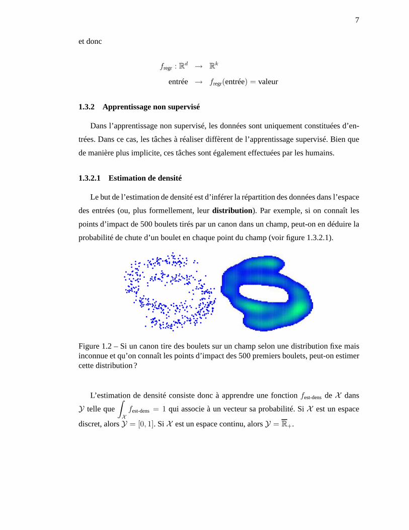
Le but de l’estimation de densité est d’inférer la répartition des données dans l’espace

des entrées (ou, plus formellement, leurdistribution ). Par exemple, si on connaît les

points d’impact de 500 boulets tirés par un canon dans un champ, peut-on en déduire la

probabilité de chute d’un boulet en chaque point du champ (voir figure 1.3.2.1).

Figure 1.2 – Si un canon tire des boulets sur un champ selon unedistribution fixe maisinconnue et qu’on connaît les points d’impact des 500 premiers boulets, peut-on estimercette distribution ?

L’estimation de densité consiste donc à apprendre une fonction fest-densdeX dans

Y telle que∫

Xfest-dens= 1 qui associe à un vecteur sa probabilité. SiX est un espace

discret, alorsY = [0, 1]. SiX est un espace continu, alorsY = R+.

8

Supposons queX est un espace continu. Alors, en reprenant la notation de l’équa-

tion 1.1, nous avons

Y = R+

et donc

fest-dens: X → R+

entrée → fest-dens(entrée) = probabilité

1.3.2.2 Regroupement (ou« clustering »)

Le regroupement est l’équivalent non supervisé de la classification. Comme son nom

l’indique, son but est de regrouper les données en classes enutilisant leurs similarités.

La difficulté du regroupement réside dans l’absence de mesure générale de similarité.

Celle-là doit donc être définie en fonction du problème à traiter. L’un des algorithmes de

regroupement les plus couramment utilisés est l’algorithme desk-moyennes.

Le regroupement consiste donc à apprendre une fonctionfregroup de Rd dansN qui

associe à un vecteur son groupe. Contrairement à la classification, le nombre de groupes

n’est pas connu a priori.

Tout comme en classification, la fonctionfregrouppeut parfois renvoyer un« vecteur

d’appartenances» dont les éléments sont positifs et somment à 1. Dans ce cas, lai-ème

composante représente le degré d’appartenance de l’entréeau groupei.

En reprenant la notation de l’équation 1.1, nous avons

X = Rd,Y = N

et donc

fregroup : Rd → N

entrée → fregroup(entrée) = groupe

9

1.3.2.3 Réduction de dimensionnalité

Les algorithmes de réduction de dimensionnalité tentent detrouver une projection

des données dans un espace de plus faible dimension, tout en préservant l’information

contenue dans celles-là. Cette projection peut être linéaire (comme dans l’analyse en

composantes principales ou ACP) ou non (par exemple les algorithmes Locally Linear

Embedding (LLE), Isomap ou l’ACP à noyau). Une étude comparative de ces algo-

rithmes peut être trouvée dans [11]. Certains de ces algorithmes ne fournissent que les

coordonnées en basse dimension (appeléescoordonnées réduites) des données d’ap-

prentissage alors que d’autres fournissent explicitementla fonction de projection, ce

qui permet de calculer les coordonnées réduites de nouveauxpoints. Toutefois, Bengio

et al. [18] présentent une méthode permettant de calculer les coordonnées réduites de

nouveaux points à partir de celles des données d’apprentissage.

La réduction de dimensionnalité consiste donc à apprendre une fonctionf de Rd

dansRk qui associe à un vecteur sa représentation en faible dimension. Si l’algorithme

est linéaire, la fonctionf sera représentée par une matrice de taille(k, n).

En reprenant la notation de l’équation 1.1, nous avons

X = Rd,Y = R

k, k < n

et donc

fdim-red : Rd → R

k

entrée → fdim-red(entrée) = coordonnées réduites

1.3.3 Apprentissage semi-supervisé

Comme son nom l’indique, l’apprentissage semi-supervisé se situe entre l’appren-

tissage supervisé et l’apprentissage non supervisé. Certaines données sont étiquetées

(c’est-à-dire sont composées d’une entrée et d’une étiquette) et d’autres ne le sont pas

(seule l’entrée est fournie). Les tâches réalisées en apprentissage semi-supervisé sont les

mêmes que celles réalisées en apprentissage supervisé (régressionetclassification), à la

10

différence qu’il est fait usage des données non étiquetées.Un exemple où l’apprentissage

semi-supervisé est adapté est la reconnaissance d’images.Il est très facile de récolter un

grand nombre d’images (sur Internet, par exemple), mais il est plus difficile (que ce soit

en termes de coûts ou de temps) de les étiqueter. Dès lors, avoir un algorithme capable

de tirer avantages des images non étiquetées pour améliorerses performances est sou-

haitable.

1.4 Entraînement, test et coûts

Dans la section 1.2, je mentionnais les étapes d’entraînement et de test associées à un

algorithme d’apprentissage. Cette section présente plus en détail les éléments nécessaires

à ces étapes.

1.4.1 Algorithmes et paramètres

La section 1.2 définit un algorithme d’apprentissage comme une fonction mathé-

matiqueA qui prend comme argument un ensemble d’exemplesD et qui renvoie une

fonctionf . Cette section explique plus en détail par quels moyens l’ensembleD influe

sur la fonctionf .

Un algorithme d’apprentissage est un modèle mathématique composé deparamètres

θ dont dépend la fonctionf finale renvoyée. Le but de l’entraînement est de trouver l’en-

semble de paramètres qui permet de réaliser au mieux la tâchesur les exemples d’en-

traînement. L’entraînement est donc uneoptimisation des paramètres. Il est intéressant

de noter qu’il existe une autre vision de l’apprentissage pour lesquels tous les jeux de

paramètres sont possibles, mais avec des probabilités différentes. L’entraînement n’est

alors plus une optimisation des paramètres mais uneestimation de cette distribution.

Cette approche, appeléeapproche bayésienne, sera brièvement traitée à la section 1.6.2

et le lecteur est renvoyé à [45] pour une introduction complète à ce modèle.

Si tous les algorithmes d’apprentissage dépendent de paramètres, on peut en extraire

deux catégories : lesalgorithmes paramètriqueset lesalgorithmes non-paramétriques.

11

1.4.1.1 Algorithmes paramétriques

Un algorithme paramétrique est un algorithme dont le nombrede paramètres et la

complexité n’augmentent pas avec la taille de l’ensemble d’entraînement. Par exemple,

un classifieur linéaire est un algorithme paramétrique puisque la fonction modélisée sera

déterminée par l’hyperplan de séparation, quelle que soit la taille de l’ensemble d’entraî-

nement.

1.4.1.2 Algorithmes non-paramétriques

Un algorithme non-paramétrique est un algorithme dont le nombre de paramètres

et la complexité augmentent avec la taille de l’ensemble d’entraînement. Un exemple

d’algorithme non-paramétrique est celui des k-plus proches voisins [20, p.125].

1.4.2 Entraînement et test

Lors de la phase d’entraînement, on veut que l’algorithme réalise une tâche prédéfinie

sur un ensemble d’exemples (l’ensemble d’entraînement), c’est-à-dire qu’il renvoie les

bonnes réponses en sortie lorsque les exemples lui sont présentés en entrée.

Il est donc important de définir :

– ce qu’est une réponse correcte

– ce qu’est une réponse incorrecte

– le coût associé à une erreur commise,

définitions qui sont propres au problème à résoudre. Ainsi, dans le cas de la reconnais-

sance d’images, confondre un 2 avec un 3 est de même importance que de confondre un

4 avec un 7. En revanche, si notre algorithme est utilisé pourdes diagnostics médicaux,

détecter une tumeur alors qu’il n’y en a pas est bien moins grave que l’inverse.

Pour apprendre à exécuter une tâche, un algorithme d’apprentissage nécessite donc :

– des données d’entraînement qui peuvent être des paires(xi, yi) (cas supervisé) ou

simplement des entréesxi (cas non supervisé)

– un coût qui représente notre définition de l’erreur.

12

Le principe le plus simple pour entraîner un algorithme d’apprentissage est la mini-

misation du coût sur les données d’entraînement : on parle d’erreur d’entraînement.

On teste ensuite notre algorithme sur de nouvelles données en calculant le coût associé :

l’ erreur de test ou erreur de généralisation. Cela permet une évaluation réaliste de la

qualité de l’algorithme.

Il est important de rappeler qu’on entraîne un algorithme enminimisant l’erreur d’en-

traînement alors que sa performance se mesure par son erreurde généralisation. Si ces

deux erreurs sont généralement liées, il existe des algorithmes qui minimisent parfai-

tement l’erreur d’apprentissage tout en ayant une erreur degénéralisation élevée (on

parlera alors desurapprentissage). La section 1.5 présente des méthodes pour limiter

ce phénomène.

1.4.3 Coûts et erreurs

Il est primordial de bien choisir le coût qu’on utilise. En effet, c’est par son inter-

médiaire qu’on informe l’algorithme de la tâche qu’on veut réaliser. Si l’algorithme doit

faire des compromis entre plusieurs erreurs, c’est le coût qui déterminera le choix final.

Les deux sous-sections suivantes présentent les coûts les plus fréquemment utilisés.

Nous appelons :

– xi ∈ X l’entrée de notrei-ème donnée d’entraînement

– yi ∈ Y l’étiquette (ou sortie désirée) de notrei-ème donnée d’entraînement, dans

le cas de l’apprentissage supervisé

– fθ la fonction induite par notre algorithme d’apprentissage avec les paramètresθ.

– c : Y × Y → R la fonction de coût.

1.4.3.1 Coût pour l’apprentissage supervisé

Pour chaque exemple d’entraînementxi, nous avons une sortie désiréeyi et une

sortie obtenuefθ(xi). Le but de l’apprentissage est de trouver les paramètresθ de notre

algorithme qui minimisent la dissimilaritéc(yi, fθ(xi)) entreyi et fθ(xi). De manière

13

plus formelle, on cherche

θ∗ = argminθ

∑

i

c [fθ(xi), yi] (1.2)

La mesure de dissimilarité (oufonction de coût) dépend du problème qu’on souhaite

résoudre. Les plus répandues sont :

– erreur quadratique :c(yi, fθ(xi)) = ‖yi − fθ(xi)‖22

– log vraisemblance negative :c(yi, fθ(xi)) = − log fθ(xi)yi

– erreur de classification :c(yi, fθ(xi)) = 1yi 6=fθ(xi) où1 est la fonction indicatrice.

L’erreur quadratique est utilisée dans les problèmes derégression. Sa non-linéarité per-

met de tolérer les faibles erreurs tout en cherchant activement à limiter les erreurs im-

portantes.

La log vraisemblance négative (LVN)est utilisée pour les problèmes de classifica-

tion. La formule est utilisée pour des algorithmes dont la sortiefθ(xi) est un vecteur dont

les composantes sont positives, somment à 1 et sont aussi nombreuses que le nombre de

classes. Laj-ème composante (c’est-à-direfθ(xi)j) représente la probabilité que l’en-

tréexi appartienne à la classej. On cherche alors à trouver les paramètresθ∗ qui, étant

données les entréesxi, maximisent la probabilité des étiquettes associéesyi :

θ∗ = argmaxθ

∏

i

P (yi|xi)

= argmaxθ

∑

i

log P (yi|xi)

= argminθ −∑

i

log P (yi|xi)

θ∗ = argminθ −∑

i

fθ(xi)yi

L’erreur de classification n’est pas utilisée pour l’apprentissage à cause de sa non-

dérivabilité par rapport àθ. On l’utilise toutefois en test comme mesure de la qualité

d’un algorithme de classification.

14

1.4.3.2 Coût pour l’apprentissage non-supervisé

Cette section (ainsi que le reste de cette thèse) ne traiterapas de la question du re-

groupement. Nous allons donc définir un coût pour l’apprentissage non-supervisé dans

le seul cadre de l’estimation de densité.

Une supposition commune est que les données sont générées indépendamment et

d’une distribution unique (iid pourindépendantes et identiquement distribuées). Cela

est faux dans certains contextes (données temporelles, spatiales, ...) qui ne seront pas

traités dans cette thèse. Nous supposerons donc désormais que nos données sont générées

de façoniid .

Dans ce cas, la vraisemblance d’un ensemble de données est égal au produit des

probabilités des éléments de cet ensemble :

Si D = x1, . . . , xN, alorsp(D) =∏

i

p(xi) (1.3)

Pour des raisons de simplicité de calcul, nous allons minimiser lalog vraisemblance

négative (LVN) au lieu de maximiser la vraisemblance en notant que cela est équivalent.

1.5 Régularisation

Un algorithme d’apprentissageA prend en entrée un ensemble deN exemples d’en-

traînementD et renvoie une fonctionA(D) = f associée.

Nos exemples d’entraînement sont tirés d’une distributionp surX × Y dans le cas

de l’apprentissage supervisé (et deX dans le cas de l’apprentissage non supervisé).

Comme mentionné à la section 1.4.3.2, cette distributionp induit une distribution sur

les ensembles d’entraînementD de tailleN (appartenant à(X × Y)N dans le cas de

l’apprentissage supervisé etXN dans le cas de l’apprentissage non supervisé) :

Si D = x1, . . . , xN, alorsp(D) =∏

i

p(xi)

Dans le cas oùA n’est pas un algorithme trivial, deux ensembles d’entraînement diffé-

15

rentsD1 etD2 donneront deux fonctions différentesf1 etf2.

Appelonsf ∗ la vraie fonction (inconnue) qu’on cherche à approcher le mieux pos-

sible. Le choix de notre algorithme d’apprentissage sera guidé par deux questions inti-

mement liées :

– en moyenne sur l’ensemble des ensembles d’entraînement possibles, notre algo-

rithme va-t-il donner la bonne réponse ?

– quelle est la sensibilité de notre algorithme à l’ensembled’entraînement particulier

qui est fourni ?

Mathématiquement, ces deux questions se traduisent par l’évaluation de deux quan-

tités : le biaisB et la varianceV . Définissons tout d’abord la fonction moyenne résultant

de notre algorithme d’apprentissage :

f = EDA(D) (1.4)

On obtient alors les formules du biais et de la variance suivantes :

B = Ex

[f(x) − f ∗(x)

](1.5)

V = ED

[Ex

[A(D)(x) − f(x)

]2](1.6)

On peut montrer [20, p.147] que l’erreur de généralisation de notre algorithme est

égale à

R = B2 + V + σ2 (1.7)

où σ représente le bruit, c’est-à-dire la partie dey qu’il est impossible de prédire, étant

donnéx.

Pour assurer une bonne généralisation, il est donc important de diminuer à la fois le

biais et la variance. Cette équation nous permet de mieux comprendre les défauts de l’ap-

prentissage par coeur. En effet, celui-là aura un biais nul mais une variance très élevée

(puisque chaque ensemble d’apprentissage différent donnera lieu à une fonction très dif-

férente) avec pour conséquence une grande erreur de généralisation. De la même façon,

un algorithme trop simple possèdera une variance faible (ayant peu de paramètres, les

16

spécificités de chaque ensemble d’entraînement n’auront que peu d’influence) mais un

biais élevé (si les fonctions générées sont trop simples, elles ne pourront bien représenter

la vraie fonctionf ∗).

L’idée de la régularisation est donc de réduire la variance de notre algorithme tout

en essayant de maintenir un biais le plus faible possible. Laméthode utilisée dépendra

donc du problème à traiter et la solution finale obtenue sera donc un compromis entre

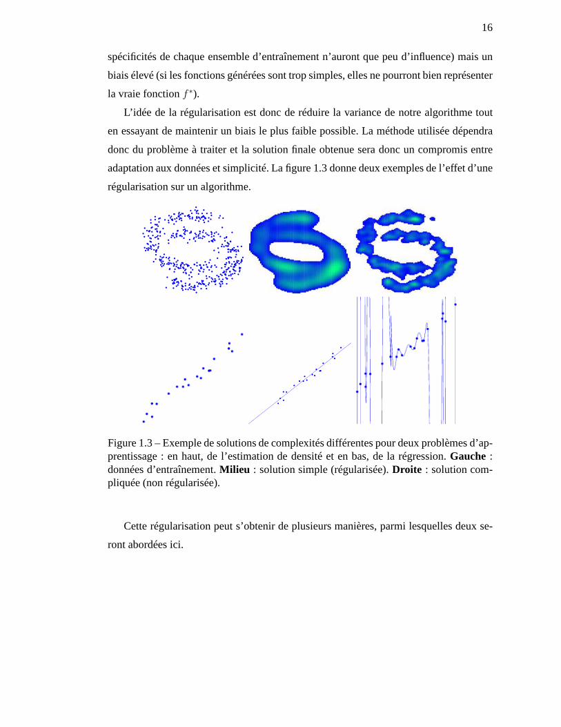
adaptation aux données et simplicité. La figure 1.3 donne deux exemples de l’effet d’une

régularisation sur un algorithme.

Figure 1.3 – Exemple de solutions de complexités différentes pour deux problèmes d’ap-prentissage : en haut, de l’estimation de densité et en bas, de la régression.Gauche :données d’entraînement.Milieu : solution simple (régularisée).Droite : solution com-pliquée (non régularisée).

Cette régularisation peut s’obtenir de plusieurs manières, parmi lesquelles deux se-

ront abordées ici.

17

1.5.1 Limitation du nombres de paramètres

Les algorithmes paramétriques possèdent une structure et un nombre de para-

mètres fixés et indépendants du nombre d’exemples d’apprentissage. Réduire le nombre

de paramètres d’un algorithme paramétrique permet d’en limiter la capacité, c’est-à-dire

le nombre de fonctions qu’il peut modéliser. Cela réduira lavariance entre les fonctions

renvoyées pour des ensembles d’apprentissage différents.Dans un réseau de neurones,

cela reviendrait par exemple à avoir un nombre réduit de neurones sur la couche cachée

(voir section 2.2).

1.5.2 Pénalisation des poids (« weight decay»)

Plutôt que de supprimer des paramètres afin d’en limiter le nombre total, on pour-

rait simplement les forcer à prendre la valeur 0. Il en résulte l’intuition qu’un paramètre

proche de 0 sera moins« actif » qu’un paramètre dont la valeur est forte. Si cette intui-

tion a des fondements théoriques (voir par exemple [60]), cette section se contente de

présenter des exemples de régularisation utilisant ce principe.

Nous allons donc ajouter au coût d’apprentissage une pénalité sur les poids (« weight

decay») que nous allons également chercher à minimiser. Le jeu de paramètres optimal

sera donc celui qui assurera un compromis entre une bonne qualité de modélisation des

données d’apprentissage (minimisation du coût empirique)et une bonne simplicité (mi-

nimisation de la pénalité). On appellecoût régulariséde l’algorithme la somme de des

deux coûts.

Cette méthode de régularisation présente l’avantage de pouvoir être appliquée tant

aux algorithmes paramétriques qu’aux algorithmes non-paramétriques, comme les mé-

thodes à noyau présentées à la section 2.1.

Les sous-sections suivantes présentent les pénalisationsles plus fréquemment ren-

contrées dans la littérature.

18

1.5.2.1 NormeL1

Soit θ l’ensemble des paramètres de notre algorithme (ou le sous-ensemble qu’on

veut régulariser). La régularisation de la normeL1 (appelée plus simplementrégulari-

sationL1) est de la formeλ‖θ‖1.

λ est appelé coefficient de régularisation (weight decay coefficient, en anglais) et sa

valeur détermine le compromis entre la simplicité que nous voulons avoir et la qualité

de la modélisation des données d’apprentissage.

Modifier un paramètre de la valeur 0 à la valeurε augmente le coût de régularisation

de λε ; cela n’est intéressant que si la dérivée du coût par rapportà ce paramètre est

supérieur àλ (en valeur absolue). La régularisationL1 encourage donc les paramètres à

être nuls. C’est pourquoi on utilise ce type de régularisation lorsqu’on veut encourager

les solutions possédant peu de paramètres non nuls. Toutefois, sa non-dérivabilité en 0

complique parfois le processus d’optimisation.

1.5.2.2 NormeL2

La régularisation de la normeL2 (ou régularisation L2) est de la formeλ2‖θ‖2

2.

La rigueur voudrait qu’elle soit appelérégularisation de la normeL2 au carré, mais

comme personne n’utilise la vraie normeL2, la simplicité y a gagné ce que la précision

y a perdu. En outre, on utilise souventλ à la place deλ2.

Modifier un paramètre de la valeur 0 à la valeurε augmente le coût de régularisation

deλε2 alors que le coût empirique varie enε ; c’est la raison pour laquelle la régularisa-

tion L2 tend à fournir des solutions dont aucun paramètre n’est nul.Toutefois, le terme

de régularisation étant différentiable, l’optimisation du coût est bien plus facile que dans

le cas de la régularisationL1.

1.5.3 Discussion

Ainsi que nous l’avons dit en préambule de cette section, le but de la régularisation

est de favoriser les fonctions simples afin de limiter la variance de notre algorithme.

19

Toute la difficulté du choix de la régularisation réside doncdans l’analogie entre la mé-

thode choisie et la notion de simplicité induite.

Tout être humain tend également à favoriser les solutions simples, comme en atteste

le rasoir d’Occam :

Pluralitas non est ponenda sine necessitate

qui pourrait être traduit par

Les multiples ne doivent pas être utilisés sans nécessité

(http ://fr.wikipedia.org/wiki/Rasoir_d’Occam)

L’une des étapes de notre quête de l’intelligence artificielle est donc de découvrir et

de modéliser la notion de simplicité que les humains utilisent. Les deux exemples de la

figure 1.3 semblent exhiber des régularités validant nos critères, mais sont-ce les seules ?

Neal [60] montra qu’il n’était pas nécessaire de limiter le nombre de neurones sur

la couche cachée d’un réseau de neurones pour se restreindreà des solutions simples,

si tant est qu’on pénalise suffisamment les paramètres de notre algorithme. Hinton et al.

[39], LeCun et al. [54] proposent des algorithmes possédantun grand nombre de para-

mètres soumis à des contraintes supplémentaires pour en limiter la capacité. Les résultats

spectactulaires obtenus par de tels algorithmes laissent penser que la notion humaine de

simplicité n’émane pas d’un nombre limité de paramètres (notre cerveau possède bien

plus de neurones que n’importe quel algorithme créé à ce jour) mais plutôt de contraintes

supplémentaires restreignant le champ des solutions possibles.

Le travail proposé dans cette thèse sera donc axé autour d’algorithmes possédant un

grand nombre de paramètres contraints de manière appropriée.

1.6 Théorème de Bayes

Nous allons maintenant présenter un théorème de grande importance en statistiques

et en apprentissage machine. Cela va nous permettre de présenter les concepts de coût et

de régularisation sous un nouveau jour. Soit le problème suivant :

Supposons qu’on connaisse la proportion d’hommes et de femmes au Ca-

nada ainsi que la distribution des tailles des individus de chaque sexe. Si un

20

Canadien choisi au hasard mesure 1m70, quelle est la probabilité que ce soit

un homme ?

Le théorème de Bayes permet de répondre à cette question. Plus formellement, il

permet de répondre à la question suivante : soit deux événements A et B. Si on connaît

a priori la probabilité que l’événement B se produise et la probabilité que l’événement

A se produise sachant que B s’est produit, peut-on en déduirela probabilité que B se

produise sachant que A s’est produit ?

Théorème 1.6.1.

P (B|A) =P (A|B)P (B)

P (A)(1.8)

Dans l’exemple ci-dessus, l’événement B est le sexe de l’individu et l’événement A

est sa taille.

Réécrivons ce théorème dans le cadre de l’apprentissage machine en précisant ce que

sont les événements A et B :

P (θ|D) =P (D|θ)P (θ)

P (D)(1.9)

Dans ce cas, nous sommes intéressés par la probabilité d’avoir un jeu de paramètres

particulierθ étant donné que nous avons à notre disposition l’ensemble d’apprentissage

D. Nous voyons que pour calculer cette probabilité, nous avons besoin de calculer trois

termes :

– P (D|θ) est la probabilité que l’ensemble d’apprentissageD ait été généré sachant

que les paramètres de l’algorithme étaientθ. Cette quantité s’appelle lavraisem-

blancede l’ensemble d’apprentissage. Cette quantité est définie par notre modèle.

– P (θ) est la probabilité a priori d’avoir comme jeu de paramètresθ. Cette quantité

s’appelle l’a priori et représente notre connaissance du monde. Elle peut être fixée

arbitrairement.

– P (D) est la probabilité d’avoir obtenu cet ensemble d’apprentissage. Elle sert sim-

plement à s’assurer que le termeP (θ|D) est bien une probabilité et somme à 1.

Elle s’appelle laconstante de normalisation.

21

Le termeP (θ|D) est appelépostérieur deθ sachantD. Il diffère de l’a prioriP (θ)

par l’information apportée parD. On voit donc que, pour qu’un jeu de paramètresθ

soit probable sachant qu’on a à notre disposition un ensemble d’apprentissageD, il faut

non seulement qu’il ait pu générer cet ensemble d’apprentissage (termeP (D|θ)), mais

également qu’il corresponde à notre vision du monde (termeP (θ)).

À partir de ce postérieur, deux stratégies sont possibles pour calculer la fonctionf :

– on peut utiliser le jeu de paramètresθ∗ le plus probable selon le postérieur pour

faire nos prédictions

f(x) = fθ∗(x) θ∗ = argmaxθP (θ|D) (1.10)

– on peut utiliser tous les jeux de paramètres possibles avecla probabilité donnée

par leur postérieur pour faire nos prédictions

f(x) =

∫

θ

fθ(x)P (θ|D) dθ (1.11)

La première approche s’appelleMaximum A Posteriori et la deuxième approche

s’appelle l’apprentissage bayésien.

1.6.1 Maximum A Posteriori

L’entraînement d’un algorithme d’apprentissage par Maximum A Posteriori (MAP)

est la procédure la plus couramment utilisée dans la communauté, notamment pour sa

simplicité. Elle consiste à trouver l’ensemble de paramètres qui est le plus probable

a posteriori, c’est-à-dire après avoir vu l’ensemble d’apprentissageD. On veut donc

trouver leθ qui maximise

P (θ|D) =P (D|θ)P (θ)

P (D)(1.12)

En ignorant le dénominateur de l’équation 1.12 (qui ne dépend pas deθ) et en prenant

l’opposé du logarithme du numérateur, on obtient que leθ∗ cherché est celui qui mini-

mise

L(θ) = − log [P (D|θ)P (θ)] (1.13)

22

par rapport àθ. L’a priori P (θ) peut être choisi arbitrairement et correspond à notre

définition d’un jeu de paramètres probable. Si cela dépend fortement du problème, les

a priori les plus fréquemment utilisés seront présentés et analysés à la section 1.6.3.

Le termeP (D|θ) est la vraisemblance de notre ensemble d’apprentissage étant donnés

les paramètres. Les modèles les plus couramment utilisés pour cette distribution sont

présentés et analysés dans la section 1.6.3. Si on utilise una priori uniforme, c’est-à-dire

qui ne privilégie pas certaines configurations de paramètres, la procédure MAP revient

à choisir le jeu de paramètres pour lequel les données sont les plus vraisemblables : on

fait alors dumaximum de vraisemblance.

Appelonsθ∗ le jeu de paramètres qui minimise le coût :

θ∗ = argminθL(θ) (1.14)

La sortiey pour un exemplex sera alors

y = fθ∗(x) (1.15)

1.6.2 Apprentissage bayésien

L’apprentissage bayésien n’essaye pas de trouver le jeu de paramètres le plus pro-

bable mais considère l’intégralité du postérieur sur les paramètres. Étant donnée une

entréex, la sortiey vaut :

y =

∫

θ

fθ(x)P (θ|D) dθ (1.16)

Le but de l’apprentissage bayésien est donc de calculer le postérieur sur les paramètres

P (θ|D) au lieu de simplement considérer leθ∗ le plus probable, comme c’est le cas lors-

qu’on fait du MAP. On ne parle plus d’optimisation des paramètres mais d’estimation

du postérieur. Cette méthode a été présentée en détail par Neal [60] et, si elle est l’ap-

proche correcte pour réaliser des prédictions, la difficulté d’estimation du postérieur né-

cessite généralement des approximations.

23

1.6.3 Interprétation bayésienne du coût

Cette section met en correspondance certains des coûts présentés à la section 1.4.3

avec des termes de vraisemblance, ainsi que les régularisations présentées à la section 1.5

avec des termes d’a priori. Pour cela, nous allons tout d’abord considérer le contexte de

l’apprentissage par MAP de la section 1.6.1. Nous appelonsL le coût que nous essayons

de minimiser

L(θ) = − log [P (D|θ)P (θ)] (1.17)

par rapport àθ.

En supposant que les données sont tirées de manière iid, comme à la section 1.4.3.2,

et en utilisant l’équation 1.3, on en déduit

− log P (D|θ) = −n∑

i=1

log P ((xi, yi)|θ) (1.18)

et le coût total s’écrit

L(θ) = −n∑

i=1

log P ((xi, yi)|θ) − log P (θ) (1.19)

Les deux prochaines sections s’intéressent au terme−n∑

i=1

log P ((xi, yi)|θ) alors que

les deux suivantes s’intéressent au terme− log P (θ).

1.6.3.1 Bruit gaussien et erreur quadratique

Soit f ∗ la vraie fonction qui a généré les données. Supposons que cesdonnées aient

été perturbées par un bruit gaussien isotrope de varianceσdI, c’est-à-dire que, pour tout

couplex, y appartenant à(X × Y), on a

y|x ∼ N(f ∗(x), σd) (1.20)

En appelantfθ la fonction générée par notre algorithme, la log-vraisemblance néga-

24

tive des données sous notre modèle est

−n∑

i=1

log P (yi|xi, θ) =n∑

i=1

‖yi − fθ(xi)‖2

2σ2d

− log Z (1.21)

oùZ est la constante de normalisation de la gaussienne et est donc independante deθ. Le

lecteur aura remarqué que le termeP ((xi, yi)|θ) de l’équation 1.19 a été remplacé par un

termeP (yi|xi, θ), c’est-à-dire qu’on a remplacé la modélisation de la densité jointe des

données par la modélisation de la densité conditionnelle. Lasserre et al. [50] discutent

de la différence entre ces deux modèles et nous invitons le lecteur à s’y référer pour

une analyse des implications de cette modification. Nous dirons simplement que celle-là

est valide dès lors que nous voulons effectivement modéliser uniquement la probabilité

conditionnelle.

Dans ce contexte, la minimisation de la log-vraisemblance négative des données est

donc égale à la minimisation de l’erreur quadratique.

1.6.3.2 Interprétation bayésienne de la log-vraisemblance négative

Dans le contexte de la classification, supposer un bruit gaussien sur les étiquettes n’a

aucun sens. Toutefois, si nous définissonsfθ comme une fonction à valeurs dansRk où

k est le nombre de classes telle que pour toutx deX , tous les éléments defθ(x) sont

positifs et somment à 1, alors on peut définir

P (y = yi|x = xi) = softmax (fθ(xi))yi(1.22)

où la fonctionsoftmax est définie par

softmax(u)i =exp(ui)∑j exp(uj)

.

On retrouve alors le coût de la log-vraisemblance négative.

25

1.6.3.3 A priori de Laplace et régularisationL1

Unedistribution de Laplace est une distribution de probabilité de la forme

P (θ) =1

Zexp

(−‖θ − µ‖

b

)

.

Nous allons supposer une moyenne nulle sur nos paramètres d’après l’analyse faite

à la section 1.5.2 liant la faible valeur des paramètres à la simplicité de la fonction en-

gendrée.

Ainsi,

P (θ) =1

Zexp

(−‖θ‖

b

)

et donc

− log P (θ) =‖θ‖b

(1.23)

et on retrouve la régularisationL1 présentée à la section 1.5.2.1 avecλ = 1b. Une valeur

élevée deλ, pénalisant grandement les paramètres, correspond donc à un a priori sur les

paramètres reserré autour de 0. Il est donc normal qu’on cherche à réduire la valeur des

paramètres si on croit fermement qu’ils doivent être proches de 0.

1.6.3.4 A priori gaussien et la régularisationL2

Supposons un a priori gaussien de moyenne 0 sur nos paramètres, c’est-à-dire

P (θ) = N (θ, 0, Σ) (1.24)

Nous allons également considérer une variance isotrope, c’est-à-dire pénalisant de ma-

nière égale tous les éléments deθ. Cette supposition est valide dans tous les algorithmes

où tous les paramètres jouent un rôle identique, ce qui sera le cas de ceux présentés

dans cette thèse. Nous avons doncΣ = σI. En supposant une moyenne nulle sur les

26

paramètres, comme à la section précédente, nous avons alors

P (θ) = N (θ, 0, σI) (1.25)

et donc

− log P (θ) =‖θ‖2

2σ2(1.26)

On retrouve la régularisationL2 présentée à la section 1.5.2.2. Là encore, par analo-

gie, on obtientλ = 1σ2 et le même raisonnement que précédemment peut être appliqué.

CHAPITRE 2

MÉTHODES À NOYAU ET RÉSEAUX DE NEURONES

Ce chapitre a pour but de présenter deux familles d’algorithmes fréquemment utili-

sées en apprentissage machine et qui posent les fondations de cette thèse.

2.1 Les méthodes à noyau

Les méthodes à noyau ont été introduites dans les années 90 etlargement utilisées

depuis lors. Schölkopf et al. [75] passent en revue de manière détaillée ce domaine. Cette

dénomination recouvre un large éventail d’algorithmes dont la particularité est d’utiliser

une fonction à noyau qui permet d’obtenir des versions non-linéaires d’algorithmes

autrement linéaires. Les plus populaires d’entre eux sont entre autres [20] :

– la régression linéaire à noyau, une extension de la régression linéaire,

– la régression logistique à noyau, une extension de la régression logistique,

– les machines à vecteurs de support, une extension des classifieurs à marge maxi-

male.

2.1.1 Principe des méthodes à noyau

Les méthodes à noyaux se fondent sur des algorithmes dont la solution peut être

écrite en fonction de produits scalaires< xi, xj > et dont la valeur en un nouveau

point x peut être écrite en fonction des produits scalaires< x, xi > où lesxi sont des

exemples d’apprentissage. Le produit canonique de l’espace euclidien est alors remplacé

par un produit scalaire dans unespace de caractéristiques(feature space) de dimension

supérieure (potentiellement infinie). En pratique, les termes< xi, xj > sont remplacés

par des termesK(xi, xj) où K est une fonction symétrique définie positive deX × XdansR appeléenoyau (parfois égalementfonction à noyau). Dans de tels algorithmes,

le choix de la fonctionK est crucial. Les plus populaires sont [77] :

– le noyau gaussien: K(xi, xj) = exp

(−(xi − xj)

T Σ−1(xi − xj)

2

)oùΣ est une

28

matrice symétrique définie positive appeléematrice de covariancechoisie ma-

nuellement (c’est donc unhyperparamètre). La matrice de covariance est sou-

vent un multiple de la matrice identité (Σ = σ2I), auquel cas la fonction de noyau

s’écritK(xi, xj) = exp

(−‖xi − xj‖2

2σ2

).

– le noyau polynomial inhomogène: K(xi, xj) = (c+ < xi, xj >)D où c est

dansR et D est dansN. c et D sont des hyperparamètres. Ce noyau est parfois

simplement appelénoyau polynomial.

– le noyau sigmoïdal: K(xi, xj) = tanh(κ < xi, xj > +ν) oùκ et ν sont dansR.

κ etν sont des hyperparamètres. Ce noyau n’est pas défini positif.

2.1.2 Espace de Hilbert à noyau reproduisant

Étant donnés un noyauK défini positif et un ensembleX , on peut définir un espace

de HilbertHk des fonctionsf de la forme

f =m∑

i=1

αiK(·, xi) (2.1)

où m est dansN, (α1, . . . , αm) est dansRm et (x1, . . . , xm) est dansXm. Le produit

scalaire dansHk est défini par

f =

m∑

i=1

αiK(·, xi)

g =

n∑

j=1

βjK(·, yj)

< f, g >Hk=

m∑

i=1

n∑

j=1

αiβjK(xi, yj) (2.2)

HK est appelé l’espace de Hilbert à noyau reproduisantassocié au noyauK. Le terme

« reproduisant» vient du fait que, pour toute paire(xi, xj) deX 2, nous avons

< K(·, xi), K(·, xj) >Hk= K(xi, xj) (2.3)

29

Une méthode à noyau appliquera d’abord une fonctionKk aux exemples d’appren-

tissage :

Kk : X → Hk

xi → K(·, xi) (2.4)

puis entraînera un modèle linéaire sur les exemples transformés, tout en maintenant une

régularisation particulière mettant en jeu les termesK(xi, xj).

2.1.3 Théorème du représentant

Le théorème du représentanta été formulé et prouvé dans [47]. Ce théorème lie

la forme du terme de régularisation dans la fonction de coût àla forme de la fonction

minimisant ce coût régularisé. La version de ce théorème proposée ici est celle trouvée

dans [77], mais d’autres variantes existent.

Theorem 2.1.1 (Théorème du représentant).SoitΩ : [0, +∞[→ R une fonction stric-

tement croissante,X un ensemble,c : (X × Y2)m → R ∪ +∞1 une fonction de coût

etHk un espace de Hilbert à noyau reproduisant.

Toute fonctionf deHk minimisant le risque régularisé

c((x1, y1, f(x1)), . . . , (xm, ym, f(xm))) + Ω(‖f‖Hk)

avec((x1, y1), . . . , (xm, ym)) dans(X × Y)m peut s’écrire sous la forme

f =m∑

i=1

αiK(·, xi) (2.5)

On notera que l’équation 2.5 ne représente pas toutes les fonctions appartenant àHk

puisqu’elle ne fait intervenir que lesxi présents dans la formule du risque.

Ce théorème permet d’écrire facilement la solution d’un problème régularisé en fonc-

1On suppose quef(x) et y appartiennent au même espaceY. Si cela n’est pas toujours vrai, parexemple dans le cas de la classification, on peut toujours s’yrapporter de manière simple.

30

tion des exemples d’apprentissage dès lors qu’on utilise une méthode à noyau. L’équa-

tion 2.5 montre que la seule inconnue est l’ensemble desαi. Même si l’algorithme est

non-paramétrique et que les éléments deHK sont de dimension infinie, sa solution op-

timale se trouve et s’exprime facilement. Cetteastuce du noyausuggère que le point

de vue d’un modèle linéaire dansHK ne sert que de justification aux méthodes à noyau

sans avoir de réel intérêt pratique.

2.1.4 Processus gaussiens

Les processus gaussiensont été abondamment expliqués dans [84] et dans [55].

Ils sont une généralisation de la distribution gaussienne multivariée aux fonctionsf de

Rd dansR. Cette généralisation se fait en définissant une distribution sur les vecteurs

f(x1)...

f(xp)

pour tout ensemble(x1, . . . , xp) de

(R

d)p

de manière cohérente. Plus préci-

sément, pour tout ensemble(x1, . . . , xp) deRp, nous avons

f(x1)...

f(xp)

|

x1

...

xp

∼ N

µ(x1)...

µ(xp)

, C(x1,...,xp)

(2.6)

où µ est lafonction moyenneet l’élément(i, j) deC(x1,...,xp) estK(xi, xj). K est ap-

pelé fonction de covariance. Un processus gaussien est donc une distribution sur les

fonctionsf .

2.2 Réseaux de neurones

Un réseau de neurones artificiel est une approximation informatique d’un réseau de

neurones biologique. Il est composé d’unités de calcul élémentaires (lesneurones for-

mels) échangeant des signaux entre elles.

Un neurone formel (simplement appelé neurone) reçoit un ensemble dem signaux

d’entrée,e1 à em. L’entrée totale du neurone est la somme de ces entrées pondérées par

31

des poidsw1 àwm ainsi que d’un biaisw0.

Le signal d’entréeE du neurone est donc égal à

E =m∑

i=1

wiei + w0 (2.7)

Le neurone transforme ensuite cette entrée en appliquant une fonctiong, appelée

fonction de transfert, sur cette entrée. Le résultat est le signal de sortie de ce neurone :

S = g(E) = g

(m∑

i=1

wiei + w0

)(2.8)

Les algorithmes d’apprentissage pour les réseaux de neurones artificiels (simplement

appelés« réseaux de neurones») ont été développés pour la première fois dans [69]

sous le termeperceptrons. Les neurones utilisés dans ces réseaux étaient ceux définis

dans [58] utilisant l’échelon de Heaviside comme fonction de transfert.

Toutefois, l’optimisation de tels réseaux était ardue, et ce n’est que dans les années

80, lorsque Rumelhart et al. [71] découvrirent la rétropropagation du gradient, que la po-

pularité des réseaux de neurones grandit. Ils ont depuis lors été utilisés dans toutes sortes

de problèmes, de la reconnaissance de caractères (par exemple dans [51]) au traitement

du langage (par exemple [12]) en passant par la chimie.

Au fil des ans, des architectures diverses et variées de réseaux de neurones appa-

rurent. On peut citer en particulier les réseaux à convolution [51], les réseaux récurrents,

les réseaux à propagation avant, les machines de Boltzmann et les machines de Boltz-

mann restreintes [43].

Les sections suivantes seront exclusivement consacrées aux réseaux à propagation

avant ; les machines de Boltzmann restreintes seront quant àelles traitées dans le cha-

pitre 9.

32

2.2.1 Les réseaux de neurones à propagation avant

Les réseaux de neurones à propagation avant (que l’on appellera simplement« ré-

seaux de neurones») sont une famille de fonctions linéaires et non-linéaires de Rd dans

Rk. Ils sont composés d’un nombre arbitraire de neurones et la connexion entre deux

neurones est dirigée.

Dans un réseau de neurones quelconque, toutes les paires de neurones peuvent être

connectées. Dans un réseau à propagation avant, les neurones sont répartis en couches

ordonnées et les connexions sont dirigées d’une couche inférieure vers une couche su-

périeure et chaque couche effectue une transformation (possiblement non-linéaire) de la

sortie des couches précédentes. Tout au long de cette thèse,nous allons considérer un cas

spécial de réseaux à propagation avant où chaque couche effectue une transformation de

la sortie de la couche directement inférieure (et non de toutes les couches inférieures,

comme dans le cas général). Cette architecture simplifiée étant largement prédominante

dans la communauté et la seule étudiée dans cette thèse, nousles appellerons simplement

de tels réseauxréseaux de neuronessans risque de confusion.

L’entrée d’un réseau de neurones est un vecteurx dansRd. La sortie de chaque unité

est une transformation (potentiellement non-linéaire) des sorties des unités de la couche

inférieure ainsi que des poids des connexions entre les deuxcouches (voir eq. 2.8). Les

paramètres d’un réseau de neurones sont les poids associés aux connexions entre les

neurones ainsi que les biais associés à chaque neurone. Dansle réseau de la figure 2.1 a

donc comme paramètres(w1, . . . , wn, c1, . . . , cn, a1, . . . , an, b). On appellera également

poids d’entrée les poids des connexions entre la couche d’entrée et la première couche

cachée,biais d’entrée les biais des neurones de la première couche cachée,poids de

sortie les poids des connexions entre la dernière couche cachée et la couche de sortie et

biais de sortieles biais des neurones de la couche de sortie.

L’optimisation de la transformation effectuée par une couche d’un réseau de neu-

rones se fait par l’apprentissage de ses poids et biais associés.

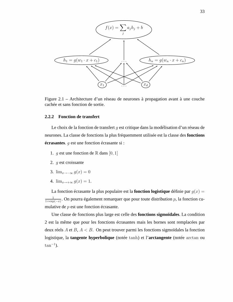
33

f(x) =∑

j

ajhj + b

h1 = g(w1 · x + c1) . . . hn = g(wn · x + cn)

x1 . . . xd

Figure 2.1 – Architecture d’un réseau de neurones à propagation avant à une couchecachée et sans fonction de sortie.

2.2.2 Fonction de transfert

Le choix de la fonction de transfertg est critique dans la modélisation d’un réseau de

neurones. La classe de fonctions la plus fréquemment utilisée est la classe desfonctions

écrasantes. g est une fonction écrasante si :

1. g est une fonction deR dans[0, 1]

2. g est croissante

3. limx→−∞ g(x) = 0

4. limx→+∞ g(x) = 1.

La fonction écrasante la plus populaire est lafonction logistiquedéfinie parg(x) =

11+exp(−x)

. On pourra également remarquer que pour toute distributionp, la fonction cu-

mulative dep est une fonction écrasante.

Une classe de fonctions plus large est celle desfonctions sigmoïdales. La condition

2 est la même que pour les fonctions écrasantes mais les bornes sont remplacées par

deux réelsA etB, A < B. On peut trouver parmi les fonctions sigmoïdales la fonction

logistique, latangente hyperbolique(notéetanh) et l’arctangente (notéearctan ou

tan−1).

34

Pour certains auteurs, les fonctions écrasantes et sigmoïdales doivent êtrecontinues

ou mêmedifférentiables. Bien que nous n’imposions pas ces restrictions, les fonctions

utilisées dans ce travail les respecteront.

2.2.3 Terminologie

Pour éviter toute confusion à la lecture de ce document, nousallons définir ici les

différentes terminologies utilisées pour décrire les réseaux de neurones :

– la couche correspondant aux vecteurs d’entrée n’est généralement pas comptée

lorsqu’on décrit un réseau de neurones. On considèrera doncque le réseau de

neurones de la figure 2.1 n’a que deux couches.

– un réseau de neurones àp couches contientp − 1 couches cachées. On pourra

donc décrire un réseau de neurones en utilisant son nombre total de couches ou

son nombre de couches cachées. Le réseau de la figure 2.1 est donc à la fois un

réseau de neurones à deux couches et un réseau de neurones à une couche cachée.

Dans cette thèse, par souci de cohérence, nous décrirons toujours un réseau de neurones

en utilisant son nombres de couches cachées.

2.2.3.1 Les réseaux de neurones et la nécessité des couches cachées

Un réseau de neurones sans couche cachée, c’est-à-dire danslequel les entrées sont

directement connectées aux sorties, ne peut discriminer les entrées que de façon linéaire.

En effet, la sortie d’un réseau de neurones sans couche cachée et avec un seul neurone

de sortie peut s’écrire sous la forme :

f(x) = g(b + w · x) (2.9)

oùb est le biais du neurone de sortie etw le vecteur de poids reliant les neurones d’entrée

au neurone de sortie. Dans le cas de la classification, la surface de décisionf(x) = c

peut donc être réécrite sous la formew · x + b = g−1(c) (si l’on suppose quec est dans

l’image deg et queg est une injection), qui est un hyperplan. Pour cette raison,des

fonctions simples comme le« ou exclusif» ne peuvent être représentées. Dans le cas de

35

la régression, s’il n’y a pas de fonction de sortie (leg de la formule 2.9), alors la sortie

est également une fonction affine de l’entrée.

Cela justifie l’utilisation de couches cachées dans les réseaux de neurones classiques.

Au vu des limitations des réseaux de neurones sans couches cachées, deux questions se

posent alors :

1. Quelles sont les limitations des réseaux de neurones aveck couches cachées ?

2. Si k0 couches cachées sont suffisantes pour modéliser n’importe quelle fonction,

est-il utile d’en avoir plus ?

2.2.3.2 Théorème de Hornik

Il existe une réponse très simple à la première question qui aété formulée et prouvée

par Hornik et al. [44] :

Theorem 2.2.1.Les réseaux de neurones multicouches à propagation avant avec une

couche cachée contenant suffisamment de neurones cachés et une fonction de transfert

écrasante arbitraire sont capable d’approcher, avec une précision arbitraire, n’importe

quelle fonction Borel-mesurable d’un espace de dimension finie dans un espace de di-

mension finie. Dans ce sens, les réseaux de neurones multicouches à propagation avant

sont une classe d’approximateurs universels.

Les réseaux de neurones classiques avec une ou plusieurs couches cachées peuvent

donc approcher arbitrairement bien toute fonction continue (le théorème prouve cette

propriété pour la classe des fonctions Borel-mesurables qui contient strictement la classe

des fonctions continues).

2.2.3.3 La nécessité de modèles hiérarchiques

Bien qu’une seule couche cachée soit nécessaire pour modéliser n’importe quelle

fonction continue, des réseaux de neurones avec plusieurs couches cachées sont éga-

lement utilisés, réalisant souvent des performances à l’état de l’art sur de nombreux

problèmes. Deux exemples de tels modèles (appelésréseaux profonds) sont les Deep

36

Belief Networks [39] et les réseaux à convolutions [51]. LesDeep Belief Networks se-

ront étudiés au chapite 9.

2.2.4 Loi a priori sur les poids et a priori sur les fonctions

La section 1.5 mentionnait le lien entre la présence d’un terme de régularisation et

les contraintes de simplicité imposées à la fonction apprise par notre algorithme. Subsé-

quemment, les sections 1.6.3.4 et 1.6.3.3 mettaient en évidence le lien entre le terme de

régularisation et l’a priori sur les paramètres d’un modèle.

Cela suggère qu’il existe un lien fort entre l’a priori sur les paramètres d’un réseau

de neurones et l’a priori sur la fonction engendrée par ce réseau. Toutefois, ce lien n’est

pas évident et [60] a étudié le cas des réseaux de neurones avec une couche cachée et

une sortie linéaire. Tous les paramètres du neurones (poidsd’entrée et de sortie, biais

d’entrée et de sortie) ont un a priori gaussien.

Pour clarifier le propos, il est nécessaire de rappeler qu’une architecture de réseau de

neurones définit une équivalence entre un jeu de paramètres et une fonction (celle induite

par un réseau de neurones possédant ces paramètres). Les sections suivantes étudient

un réseau de neurones avec un seul neurone d’entrée et un seulneurone de sortie. La

fonction induite par ce réseau sera donc deR dansR.

2.2.4.1 Loi a priori sur les poids et les biais de sortie

Il y a peu à dire sur le lien entre l’a priori sur les poids de sortie et l’a priori sur la

fonction induite. En effet, celui-là contrôle simplement l’amplitude de la sortie. Toute-

fois, il est important de remarquer que, pour maintenir l’amplitude de la sortie constante

lorsque le nombre d’unités cachées tend vers l’infini, la variance de l’a priori gaussien

sur les poids de sortie doit varier selon la racine carrée de l’inverse du nombre d’unités

cachées et la variance de l’a priori sur le biais de sortie doit rester inchangée [60].

37

2.2.4.2 A priori sur les poids et les biais d’entrée

L’a priori sur les poids d’entrée a une influence bien différente sur la fonction induite

par le réseau de neurones. En effet, [60] montra qu’un a priori fort (c’est-à-dire avec une

faible variance) sur les poids d’entrée engendrait des fonctions très lisses tandis qu’un a

priori faible (permettant aux poids de prendre des valeurs très élévées) donnait lieu à des

fonctions accidentées (voir figure 2.2).

2.2.4.3 Résumé et exemples

Le lien entre l’a priori sur les paramètres d’un réseau de neurones à une couche

cachée avec une sortie linéaire et la fonction induite par ceréseau peuvent donc être

résumés ainsi :

1. l’a priori sur les poids de sortie contrôle l’amplitude générale de la fonction in-

duite. Un a priori fort entraînera des valeurs de sortie proches de 0 tandis qu’un a

priori faible entraînera de valeurs de sorties élevées

2. l’a priori sur les poids d’entrée contrôle la rugosité de la fonction induite. Un a

priori fort entraînera des fonctions lisses tandis qu’un a priori faible entraînera des

fonctions accidentées.

La figure 2.2 présente des fonctions induites par un réseau deneurones avec un neu-

rone d’entrée, 10000 neurones cachés et un neurone de sortiedont les paramètres ont été

tirés selon une loi gaussienne.

– L’a priori sur les poids et le biais de sortie est une gaussienne de variance fixe.

– L’a priori sur les poids et biais d’entrée est une gaussienne de variancesσ =

1, 5, 20 and100.

Chaque graphique contient quatre fonctions induites pour chaque valeur deσ.

2.2.5 Liens entre les machines à noyau et les réseaux de neurones

Neal [60] prouva qu’un réseau de neurones à une couche cachéedont le nombre de

neurones cachés tend vers l’infini converge vers un processus gaussien dont la fonction

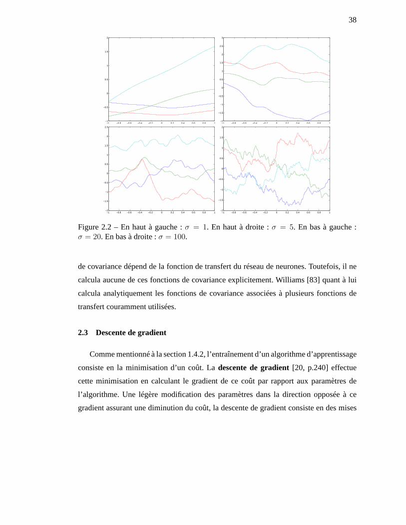
38

−1 −0.8 −0.6 −0.4 −0.2 0 0.2 0.4 0.6 0.8 1−1

−0.5

0

0.5

1

1.5

2

−1 −0.8 −0.6 −0.4 −0.2 0 0.2 0.4 0.6 0.8 1−2

−1.5

−1

−0.5

0

0.5

1

1.5

2

2.5

3

−1 −0.8 −0.6 −0.4 −0.2 0 0.2 0.4 0.6 0.8 1−2

−1.5

−1

−0.5

0

0.5

1

1.5

2

2.5

−1 −0.8 −0.6 −0.4 −0.2 0 0.2 0.4 0.6 0.8 1−2

−1.5

−1

−0.5

0

0.5

1

1.5

2

Figure 2.2 – En haut à gauche :σ = 1. En haut à droite :σ = 5. En bas à gauche :σ = 20. En bas à droite :σ = 100.

de covariance dépend de la fonction de transfert du réseau deneurones. Toutefois, il ne

calcula aucune de ces fonctions de covariance explicitement. Williams [83] quant à lui

calcula analytiquement les fonctions de covariance associées à plusieurs fonctions de

transfert couramment utilisées.

2.3 Descente de gradient

Comme mentionné à la section 1.4.2, l’entraînement d’un algorithme d’apprentissage

consiste en la minimisation d’un coût. Ladescente de gradient[20, p.240] effectue

cette minimisation en calculant le gradient de ce coût par rapport aux paramètres de

l’algorithme. Une légère modification des paramètres dans la direction opposée à ce

gradient assurant une diminution du coût, la descente de gradient consiste en des mises

39

à jour successives des paramètres de la forme

θt+1 = θt − εt∂L∂θ

(2.10)

où ε est le taux d’apprentissage. Une diminution progressive dece taux [22, 23] assure

la convergence vers un minimumlocal.

Les méthodes de second ordre utilisent une formule de mise à jour impliquant une

matriceM :

θt+1 = θt − εtM∂L∂θ

(2.11)

Les matricesM les plus fréquemment utilisées sont l’inverse de la hessienne (méthode

deGauss-Newton) ou la matrice de covariance des gradients (gradient naturel).

L’apprentissage par descente de gradient pour les réseaux de neurones a été rendu

possible grâce à la découverte de la rétropropagation du gradient [52, 71] qui permet de

calculer aisément le gradient du coût par rapport aux paramètres d’une couche du réseau

en fonction du gradient du coût par rapport aux paramètres dela couche supérieure.

CHAPITRE 3

PRÉSENTATION DU PREMIER ARTICLE

3.1 Détails de l’article

The Curse of Highly Variable Functions for Local Kernel Machines

Y. Bengio, O. Delalleau et N. Le Roux

Publié dansAdvances in Neural Information Processing Systems 18, MIT Press, Cam-

bridge, MAen 2006.

3.2 Contexte

Les méthodes à noyau ont joui d’une grande popularité depuisl’introduction des ma-

chines à vecteurs de support dans les années 90 [21, 29, 75]. Cette popularité s’explique

par deux facteurs :

– la convexité de leur optimisation

– leur capacité à modéliser n’importe quelle fonction (propriété d’approximation

universelle).

Malheureusement, ces propriétés désirables ont un coût. Ainsi, toutes les méthodes à

noyau prédéfinissent une mesure de similarité (implicitement déterminée par la fonction

à noyau choisie, voir section 2.1.1) qu’ils utilisent pour comparer les exemples de test

avec ceux d’apprentissage. Ce sont donc des« détecteurs de motif» améliorés qui ne

font que chercher dans une base de données (l’ensemble d’entraînement) les exemples

similaires (selon la mesure définie) à celui qui est testé.

Il serait toutefois inapproprié de négliger les méthodes à noyau pour cette raison.

En effet, cette limitation ne les empêche pas d’obtenir des résultats plus qu’honorables

sur de nombreux problèmes. Toutefois, dès lors que le problème possède de nombreux

degrés de variation, le nombre d’exemples d’apprentissagenécessaires pour que la dé-

tection de motifs soit efficace devient prohibitif.

41

3.3 Commentaires

Ce sont ces problèmes que l’article présenté ici formalise de plusieurs façons :

– l’erreur de généralisation de telles méthodes peut converger aussi lentement que

n− 44+d (avecn le nombre d’exemples etd la dimension de la variété à laquelle ils

appartiennent)

– le nombre de gaussiennes (de même variance) nécessaires pour apprendre une

surface de décision augmente linéairement avec le nombre derégions de même

signe

– le plan tangent à la variété apprise par une méthode à noyau utilisant un noyau local

n’est défini que comme une combinaison linéaire d’un faible nombre de points

voisins.

Cet article permet donc de mieux comprendre les raisons des faiblesses inhérentes

aux méthodes à noyau couramment utilisées ainsi que de démontrer la nécessité de l’ex-

traction de concepts dès lors que la dimensionnalité des données devient importante et

que ces dernières n’occupent qu’une partie extrêmement réduite de l’espace total.

Toutefois, notre argumentaire a ses limites. Nous nous sommes limités aux méthodes

utilisant des noyaux locaux, excluant notamment le noyau polynomial. De plus, le théo-

rème 4.5.1 se limite à des ensembles de gaussiennes de même variance, ce qui n’est pas

toujours le cas. Cependant, ces cas simplifiés sont ceux fréquemment utilisés dans la

communauté, accréditant les arguments avancés.

CHAPITRE 4

THE CURSE OF HIGHLY VARIABLE FUNCTIONS FOR LOCAL KERNEL

MACHINES

4.1 Abstract

We present a series of theoretical arguments supporting theclaim that a large class

of modern learning algorithms based on local kernels are sensitive to the curse of dimen-

sionality. These include local manifold learning algorithms such as Isomap and LLE,

support vector classifiers with Gaussian or other local kernels, and graph-based semi-

supervised learning algorithms using a local similarity function. These algorithms are

shown to be local in the sense that crucial properties of the learned function atx depend

mostly on the neighbors ofx in the training set. This makes them sensitive to the curse

of dimensionality, well studied for classical non-parametric statistical learning. There

is a large class of data distributions for which non-local solutions could be expressed

compactly and potentially be learned with few examples, butwhich will require a large

number of local bases and therefore a large number of training examples when using a

local learning algorithm.

4.2 Introduction

A very large fraction of the recent work in statistical machine learning has been

focused on so-called kernel machines, which are non-parametric learning algorithms

in which the learned function is expressed in terms of a linear combination of kernel

functions applied on the training examples :

f(x) = b +

n∑

i=1

αiK(x, xi) (4.1)

where optionally a bias termb is added,D = x1, . . . , xn are training examples (wi-

thout the labels, in the case of supervised learning), theαi’s are scalars chosen by the

43

learning algorithm using labelsy1, . . . , yn, andK(·, ·) is the kernel function, a sym-

metric function (generally expected to be positive definite). We refer to then× n matrix

M with entriesMij = K(xi, xj) as the Gram matrix. A typical kernel function is the

Gaussian kernel,

K(u, v) = e−1

σ2 ||u−v||2, (4.2)

with hyper-parameterσ (the width) controlling how local the kernel is. The Gaussian

kernel is part of a larger family of kernels which we call local kernels and discuss in

section 4.6.

Examples of kernel-based nonlinear manifold learning algorithms include Locally

Linear Embedding (LLE) [70], Isomap [79], kernel PCA (kPCA)[76], Laplacian Ei-

genmaps [8], and Manifold Charting [24]. This framework also includes spectral clus-

tering algorithms (see [81] for more references). For thesealgorithms,f represents the

embedding function, which maps an examplex to one of the coordinates of its low-

dimensional representation embedding (and a separate set of αi’s is used for each dimen-

sion of the embedding). As shown in [11], theαi correspond to entries in an eigenvector

of the Gram matrix, divided by the corresponding eigenvalue(following the Nyström

formula [6, 63, 85]). Note that these algorithms employ a special kind of kernel which is

data-dependent [11], but the arguments presented in sections 4.6, 4.7 and 4.9 also apply.

Among the statistical classifiers most widely studied in therecent years is the Sup-

port Vector Machine (SVM) [21, 29, 75], in whichf above is the discriminant function

of a binary classifier, i.e. the decision function is given bythe sign off . Since this is

a supervised learning algorithm, the training data includes a set of +1 or -1 class la-

belsy1, . . . , yn for training examples. Results in section 4.5 apply to SVMs and other

kernel machines with Gaussian kernels, and a more general conjecture is developed in

section 4.9 based on thelocal-derivativenotion introduced in section 4.7.

Another class of kernel algorithms that is discussed here are the non-parametric

graph-based semi-supervised algorithms of the type described in recently proposed pa-

pers [7, 30, 89, 90]. They can be intuitively understood as performing some kind of

smoothing or label propagation on the empirical graph defined by the examples (nodes)

44

and a similarity function (e.g. a kernel) between pairs of examples. The results in sec-

tion 4.8 are specifically tailored to such algorithms, and show that the number of required

labeled examples grows linearly with a measure of the amountof local variation of the

predictor required to reach a given error level.

The basic ideas behind the arguments presented in this paperare simple. One class of

arguments relies on showing that some important property off(x) is mostly determined

by the neighbors ofx in the training set. If one imagines tiling the space with such neigh-

borhoods, the required number of neighborhoods (hence of training examples) could

grow exponentially with the dimensionality of the data (or of the manifold on which

they live). One issue in this respect is the size of these neighborhoods, and we get ins-

piration from the classical bias-variance trade-off argument for classical non-parametric

models : if we make the regions smaller, bias is reduced (morecomplex functions can be

represented) but variance is increased (not enough data areused to determine the value

of f(x) aroundx, sof(x) becomes less stable).

Another class of arguments considers “apparently complicated” target functions, in

the sense that they vary a lot across space, although there might exist simple and com-

pact representations for them that could not be discovered using a purely local represen-

tation (eq. 4.1). For these arguments one attempts to find lower bounds on the number

of examples required in order to learn the target function. These arguments show that

whatever the method used to estimate theαi’s, one must have a large number of them

in order to approximate the function at a given set of points (larger than the size of the

training set), i.e. in order to get meaningful generalization.

In general, what one should keep in mind is that what matters is not the dimension of

the data or of the manifold near which they are found, but rather the “apparent complexi-

ty” of the function that we are trying to learn (or one that would yield an acceptable error

level). By “apparent complexity” we mean a measure of the number of “variations” of

that function. One way to formalize this notion, used in Proposition 4.8.1, is the number

of regions with constant sign of the predictor.

45

4.3 The Curse of Dimensionality for Classical Non-Parametric Models

The curse of dimensionality has been coined by Bellman [9] in the context of

control problems but it has been used rightfully to describethe poor generalization per-

formance of local non-parametric estimators as the dimensionality increases.

4.3.1 The Bias-Variance Dilemma

This problem has often been studied by considering the classical bias-variance ana-

lyses of statistical estimators. To keep the analysis simple, one usually only computes

the conditional bias and conditional variance, in the case of supervised learning, i.e. gi-

ven thexi’s of the training set, and integrating only over theyi’s. Biasof the estimator is

the expected difference between the estimator and the target function, whilevarianceof

the estimator is the expected squared difference between the estimator and its expected

value (in both cases the expectations are over the training set or over theyi’s only). The

expected mean squared error of the estimator can be shown to be equal to the sum of

variance and squared bias (plus the irreducible component of variation ofY givenX,

i.e. noise).

Two classical non-parametric estimators are worth discussing here. The first one is

thek-nearest-neighbors estimator. It can be cast as a kernel machine (eq. 4.1) whenK is

allowed to be data-dependent :αi = yi andK(x, xi) is 1/k if xi is one of thek nearest

neigbors ofx in D, 0 otherwise. The second one is the Nadaraya-Watson estimator (also

known as the Parzen windows estimator), in which againαi = yi andK(x, xi) is a

normalized kernel (i.e. also data-dependent), e.g.

K(x, xi) =K(x, xi)∑n

j=1 K(x, xj).

Since both estimators have the same form, much of the analysis can be shared. Let

t be the target function that we are trying to learn, withE[Y |X = x] = t(x). The

46

conditional bias is simply

conditional bias(x) = E[Y |X = x] −n∑

i=1

E[Y |X = xi]K(x, xi). (4.3)

Clearly, the more local the kernel (i.e.K(x, xi) is nearly 0 except forxi very close tox),

the smaller the bias (note that we consider here kernelsK such that∑

i K(x, xi) = 1).

Assuming thatV ar[yi|xi] = v does not depend onxi the conditional variance of the

estimator is

conditional variance(x) = v

n∑

i=1

K(x, xi)2.

For example, with thek-nearest neighbors estimator,

conditional variance(x) =v

k.

Clearly, the way to reduce variance is to decrease the kernel’s locality (e.g. increaseσ in

a Gaussian kernel ork in ak-nearest neighbors estimator), which increases the effective

number of examples used to obtain a prediction atx. But this also increases bias, by

making the prediction smoother (possibly too smooth). Since total error involves the

sum of squared bias and variance, one should choose the kernel hyper-parameter (e.g.k

or σ) to strike the best balance (hence thebias-variance dilemma[35]).

4.3.2 Dimensionality and Rate of Convergence

A nice property of classical non-parametric estimators is that one can prove their

convergence to the target function asn → ∞, i.e. these are consistent estimators. Consi-

dering the above simplified exposition on bias and variance,one obtains consistency by

appropriately varying the hyper-parameter that controls the locality of the estimator as

n increases. Basically, the kernel should be allowed to become more and more local, so

that bias goes to zero, but the “effective number of examples” involved in the estimator

atx,1∑n

i=1 K(x, xi)2

47

(equal tok for thek-nearest neighbors estimator) should increase asn increases, so that

variance is also driven to 0. For example one obtains this condition with limn→∞ k = ∞and limn→∞

kn

= 0 for the k-nearest neighbor. Clearly the first condition is sufficient

for variance to go to 0 and the second is sufficient for the biasto go to 0 (sincekn

is

proportional to the volume of space aroundx which contains thek nearest neighbors).

Similarly, for the Nadarya-Watson estimator with bandwidthσ, consistency is obtained if

limn→∞ σ = 0 andlimn→∞ nσ = ∞ (in addition to regularity conditions on the kernel).

See [36] for a recent and easily accessible exposition (web version available).

The bias is due to smoothing the target function over the volume covered by the ef-

fective neighbors (consider eq. 4.3). As the intrinsic dimensionality of the data increases

(the number of dimensions that they actually span locally),bias increases. Since that

volume increases exponentially with dimension, the effectof the bias quickly becomes

very severe. To see this, consider the classical example of the [0, 1]d hypercube inRd

with uniformly distributed data in the hypercube. To hold a fractionp of the data in a

sub-cube of it, that sub-cube must have sides of lengthp1/d. As d → ∞, p1/d → 1, i.e.

we are averaging over distances that cover almost the whole span of the data, just to keep

variance constant (by keeping the effective number of neighbors constant).

When the input examples are not considered fixed the calculations of bias and va-

riance are more complex, but similar conclusions are reached. For example, for a wide

class of such kernel estimators, the unconditional variance and squared bias can be

shown to be written as follows [36] :

expected error =C1

nσd+ C2σ

4,

(where the expected error is the sum of the variance and the squared bias of the estimator)

with C1 andC2 not depending onn nord. Hence an optimal bandwidth is chosen propor-

tional ton−14+d , and the resulting generalization error (not counting the noise) converges

in n−4/(4+d), which becomes very slow for larged. Consider for example the increase

in number of examples required to get the same level of error,in 1 dimension versus

d dimensions. Ifn1 is the number of examples required to get a level of errore, to get

48

the same level of error ind dimensions requires on the order ofn(4+d)/51 examples, i.e.

the required number of examples is exponential ind. However, if the data distribu-

tion is concentrated on a lower dimensional manifold, it is themanifold dimension that

matters. Indeed, for data on a smooth lower-dimensional manifold, the only dimension

that, say, ak-nearest neighbors classifier sees is the dimension of the manifold, since it

only uses the Euclidean distances between the near neighbors, and if they lie on such a

manifold then the local Euclidean distances approach the local geodesic distances on the

manifold [79].

4.4 Summary of the results

In the following sections, we will see that :

– In the case of a Gaussian kernel machine classifier, if there exists a line inRd

that intersectsm times with the decision surfaceS (and is not included inS), one

needs at least⌈m2⌉ Gaussians (of same width) to learnS.

– At least2d−1 examples are required to represent thed-bit parity (the function from

0, 1d to −1, 1 which is1 iff the sum of the bits is even), when using Gaussians

with fixedσ centered on data points.

– Many graph-based semi-supervised learning algorithms cannot learn a number of

regions with constant label higher than the number of labeled examples.

– When the test examplex is far from all thexi, a predictor given by eq. 4.1 with

a local kernel either converges to a constant or a nearest neighbors classifier.

Neither of these are good in high dimension.

– When using so-called local-derivative kernels,∂f(x)∂x

is constrained to be approxi-

mately a linear combination of the vectors(x − xi) with xi a near neighbor ofx.

In high dimension (when the number of effective neighbors issignificantly smal-

ler than the dimension), this is a very strong constraint (either on the shape of the

manifold or of the decision surface).

– When there are examples with||x − xi|| near σ (which is likely to happen for

“good” values of σ, i.e. neither too small nor too big), withx on the decision

49

surface, small changes inx w.r.t. σ yield only small changes in the normal vector

of the decision surface.The above statement is one about bias : within a ball of

radiusσ, the decision surface is constrained to be smooth (small changes inx yield

small changes in the shape of the surface).

– In the case of a Gaussian kernel classifier, whenσ increases the decision surface

becomes subject to specific smoothness constraints.More generally, we present

an argument supporting the conjecture that any learning algorithm with a local

property, such as thelocal-derivative property(∂f∂x

depends mostly on examples

in a ball aroundx) and local smoothness of the learned function (e.g., withinthat

ball) will be subject to the curse of dimensionality.

These statements highlight some important limitations of kernel methods, that one must

keep in mind when applying such learning algorithms.

4.5 Minimum Number of Bases Required for Complex Functions

4.5.1 Limitations of Learning with Gaussians

In [74] tight bounds are established for the number of zeros of univariate radial basis

function networks under certain parameter conditions. In particular, it is shown that for

a fixed Gaussian widthσ, a function

f : R → R

of the form

f(x) = b +

k∑

i=1

αi exp

(−‖x − xi‖2

σ2

)(4.4)

cannot have more than2k zeros (if there is at least one non-zeroαi). Consider now the

more general case of a multivariate decision functionf : Rd → R written as in eq. 4.4.

For anyu ∈ Rd and anyw ∈ R

d such that‖w‖ = 1, the functiong : R → R defined by

g(t) = f(u + tw)

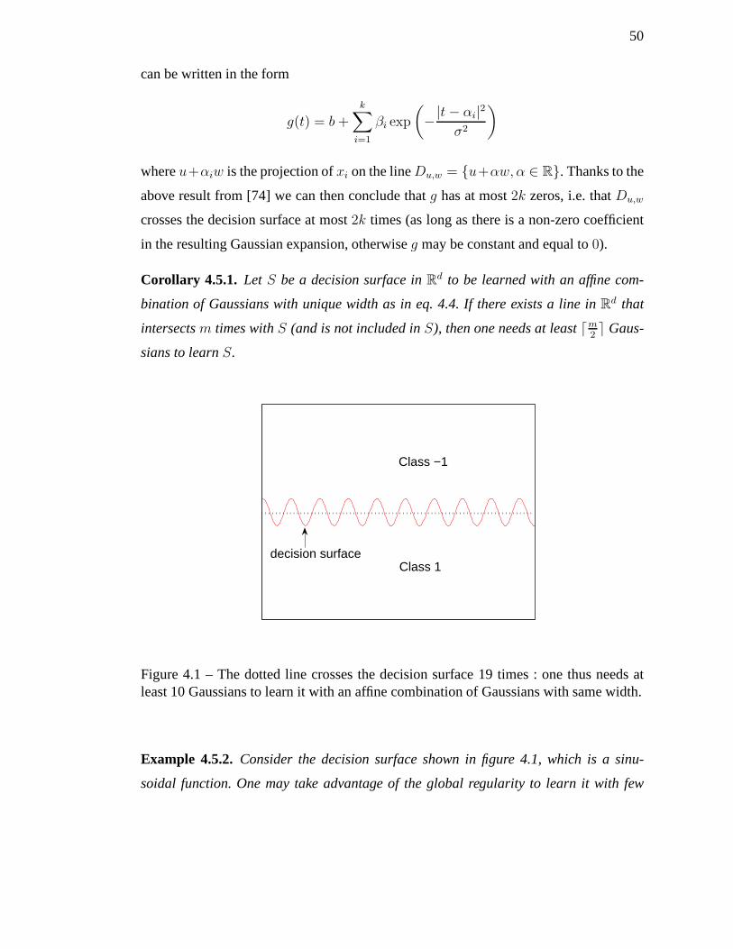
50

can be written in the form

g(t) = b +

k∑

i=1

βi exp

(−|t − αi|2

σ2

)

whereu+αiw is the projection ofxi on the lineDu,w = u+αw, α ∈ R. Thanks to the

above result from [74] we can then conclude thatg has at most2k zeros, i.e. thatDu,w

crosses the decision surface at most2k times (as long as there is a non-zero coefficient

in the resulting Gaussian expansion, otherwiseg may be constant and equal to0).

Corollary 4.5.1. Let S be a decision surface inRd to be learned with an affine com-

bination of Gaussians with unique width as in eq. 4.4. If there exists a line inRd that

intersectsm times withS (and is not included inS), then one needs at least⌈m2⌉ Gaus-

sians to learnS.

decision surface

Class −1

Class 1

Figure 4.1 – The dotted line crosses the decision surface 19 times : one thus needs atleast 10 Gaussians to learn it with an affine combination of Gaussians with same width.

Example 4.5.2.Consider the decision surface shown in figure 4.1, which is a sinu-

soidal function. One may take advantage of the global regularity to learn it with few

51

parameters (thus requiring few examples), but with an affinecombination of Gaussians,

corollary 4.5.1 implies one would need at least⌈m2⌉ = 10 Gaussians. For more complex

tasks in higher dimension, the “complexity” of the decisionsurface could quickly make

learning impractical when using such a local kernel method.

Remark 4.5.3. Of course, one only seeks to approximate the decision surface S, and

does not necessarily need to learn it perfectly : corollary 4.5.1 says nothing about the

existence of an easier-to-learn decision surface approximating S. For instance, in the

example of figure 4.1, the dotted line could turn out to be a good enough estimated

decision surface if most samples were far from the true decision surface, and this line

can be obtained with only two Gaussians.

4.5.2 Learning thed-Bits Parity Function

Thed-bits parity function is the function

parity : (b1, . . . , bd) ∈ 0, 1d 7→

1 if∑d

i=1 bi is even

−1 otherwise

We will show that learning this apparently simple function with Gaussians centered on

points in0, 1d is difficult, in the sense that it requires a number of Gaussians exponen-

tial in d (for a fixed Gaussian width). We will use the following notations :

Xd = 0, 1d = x1, x2, . . . , x2dH0

d = (b1, . . . , bd) ∈ Xd | bd = 0 (4.5)

H1d = (b1, . . . , bd) ∈ Xd | bd = 1

Kσ(x, y) = exp

(−‖x − y‖2

σ2

)

We say that a decision functionf : Rd → R solves the parity problem ifsign(f(xi)) =

parity(xi) for all i in 1, . . . , 2d.

Lemma 4.5.4. Let f(x) =∑2d

i=1 αiKσ(xi, x) be a linear combination of Gaussians

52

with same widthσ centered on pointsxi ∈ Xd. If f solves the parity problem, then

αiparity(xi) > 0 for all i.

Démonstration.We prove this lemma by induction ond. If d = 1 there are only 2 points.

Obviously one Gaussian is not enough to classify correctlyx1 andx2, so bothα1 andα2

are non-zero, andα1α2 < 0 (otherwisef is of constant sign). Without loss of generality,

assumeparity(x1) = 1 andparity(x2) = −1. Thenf(x1) > 0 > f(x2), which implies

α1(1 − Kσ(x1, x2)) > α2(1 − Kσ(x1, x2)) andα1 > α2 sinceKσ(x1, x2)) < 1. Thus

α1 > 0 andα2 < 0, i.e.αiparity(xi) > 0 for i ∈ 1, 2.

Suppose now lemma 4.5.4 is true ford = d′−1, and consider the cased = d′. We denote

by x0i the points inH0

d and byα0i their coefficient in the expansion off (see eq. 4.5 for

the definition ofH0d ). Forx0

i ∈ H0d , we denote byx1

i ∈ H1d its projection onH1

d (obtained

by setting its last bit to 1), whose coefficient inf is α1i . For anyx ∈ H0

d andx1j ∈ H1

d we

have :

Kσ(x1j , x) = exp

(−‖x1

j − x‖2

σ2

)

= exp

(− 1

σ2

)exp

(−‖x0

j − x‖2

σ2

)

= γKσ(x0j , x)

whereγ = exp(− 1

σ2

)∈ (0, 1). Thusf(x) for x ∈ H0

d can be written

f(x) =∑

x0i ∈H0

d

α0i Kσ(x0

i , x) +∑

x1j∈H1

d

α1jγKσ(x0

j , x)

=∑

x0i ∈H0

d

(α0

i + γα1i

)Kσ(x0

i , x)

SinceH0d is isomorphic toXd−1, the restriction off to H0

d implicitely defines a function

overXd−1 that solves the parity problem (because the last bit inH0d is 0, the parity is not

modified). Using our induction hypothesis, we have that for all x0i ∈ H0

d :

(α0

i + γα1i

)parity(x0

i ) > 0. (4.6)

53

A similar reasoning can be made if we switch the roles ofH0d andH1

d . One has to be

careful that the parity is modified betweenH1d and its mapping toXd−1 (because the last

bit in H1d is 1). Thus we obtain that the restriction of(−f) to H1

d defines a function over

Xd−1 that solves the parity problem, and the induction hypothesis tells us that for all

x1j ∈ H1

d :(−(α1

j + γα0j

)) (−parity(x1

j ))

> 0. (4.7)

and the two negative signs cancel out. Now consider anyx0i ∈ H0

d and its projection

x1i ∈ H1

d . Without loss of generality, assumeparity(x0i ) = 1 (and thusparity(x1

i ) =

−1). Using eq. 4.6 and 4.7 we obtain :

α0i + γα1

i > 0

α1i + γα0

i < 0

It is obvious that for these two equations to be simultaneously verified, we needα0i and

α1i to be non-zero and of opposite sign. Moreover,α0

i +γα1i > 0 > α1

i +γα0i ⇒ α0

i > α1i ,

which impliesα0i > 0 andα1

i < 0, i.e.α0i parity(x0

i ) > 0 andα1i parity(x1

i ) > 0. Since

this is true for allx0i in H0

d , we have proved lemma 4.5.4.

Theorem 4.5.5.Letf(x) = b+∑2d

i=1 αiKσ(xi, x) be an affine combination of Gaussians

with same widthσ centered on pointsxi ∈ Xd. If f solves the parity problem, then there

are at least2d−1 non-zero coefficientsαi.

Démonstration.We begin with two preliminary results. First, given anyxi ∈ Xd, the

number of points inXd that differ fromxi by exactlyk bits is(

dk

). Thus,

∑

xj∈Xd

Kσ(xi, xj) =d∑

k=0

(d

k

)exp

(−k2

σ2

)= cσ. (4.8)

Second, it is possible to find a linear combination (i.e. without bias) of Gaussiansg such

54

thatg(xi) = f(xi) for all xi ∈ Xd. Indeed, let

g(x) = f(x) − b +∑

xj∈Xd

βjKσ(xj , x). (4.9)

g verifiesg(xi) = f(xi) iff∑

xj∈XdβjKσ(xj , xi) = b, i.e. the vectorβ satisfies the linear

systemMσβ = b1, whereMσ is the kernel matrix whose element(i, j) is Kσ(xi, xj)

and1 is a vector of ones. It is well known thatMσ is invertible as long as thexi are

all different, which is the case here [59]. Thusβ = bM−1σ 1 is the only solution to the

system.

We now proceed to the proof of the theorem. By contradiction,supposef(x) = b +∑2d

i=1 αiKσ(xi, x) solves the parity problem with less than2d−1 non-zero coefficients

αi. Then there exist two pointsxs andxt in Xd such thatαs = αt = 0 andparity(xs) =

1 = −parity(xt). Consider the functiong defined as in eq. 4.9 withβ = bM−1σ 1. Since

g(xi) = f(xi) for all xi ∈ Xd, g solves the parity problem with a linear combination of

Gaussians centered points inXd. Thus, applying lemma 4.5.4, we have in particular that

βsparity(xs) > 0 andβtparity(xt) > 0 (becauseαs = αt = 0), so thatβsβt < 0. But,

because of eq. 4.8,Mσ1 = cσ1, which means1 is an eigenvector ofMσ with eigenvalue

cσ > 0. Consequently,1 is also an eigenvector ofM−1σ with eigenvaluec−1

σ > 0, and

β = bM−1σ 1 = bc−1

σ 1, which is in contradiction withβsβt < 0 : f must have at least

2d−1 non-zero coefficients.

Remark 4.5.6.The bound in theorem 4.5.5 is tight, since it is possible to solve the parity

problem with exactly2d−1 Gaussians and a bias, for instance by using a negative bias

and putting a positive weight on each example satisfyingparity(x) = 1.

Remark 4.5.7. When trained to learn the parity function, a SVM may learn a function

that looks like the opposite of the parity on test points (while still performing optimally on

training points). For instance, a SVM trained with4000 unique points fromX15 achieves

a 90% error rate on 20000 different test samples (withσ = 0.5). This is because a

bit less than90% of these test samples are at distance 1 from their nearest neighbor

in the training set. With this value ofσ, the SVM output is similar to nearest neighbor

55

classification, which is wrong when the nearest neighbor is at distance 1. However, this

observation cannot in general be used to build a model for parity with Gaussians (by

taking the opposite of the SVM output) : indeed, this approach would work here because

the training samples are dense enough inX15, but this will not be the case with fewer

training data or in higher dimensions. Note that in all our experiments performed with

parity datasets, a SVM had a50% or more error rate on new points, which illustrates its

inability to generalize for this problem.

Remark 4.5.8. If the centers of the Gaussians are not restricted anymore tobe points

in Xd, it is possible to solve the parity problem with onlyd + 1 Gaussians and no bias.

Indeed, considerf defined by

f(x) =

d∑

i=0

(−1)iKσ(yi, x)

with

yi =i

d1.

For σ small enough,sign(f(yi)) = (−1)i. In addition, for anyx ∈ Xd, f(x) =

γf(x), where x is the projection ofx on the diagonal (the line spanned by1) and

γ = exp(−‖x−x‖2

σ2

)∈ (0, 1). Letx = (b1, . . . , bd) : its projectionx is given by

x = (x · 1)1

‖1‖2=

1

d

(∑

i

bi

)1 = y(

Pi bi)

and thereforesign(f(x)) = sign(f(x)) = sign(f(y(

Pi bi)

))= (−1)(

Pi bi) = parity(x) :

f solves the parity problem with a linear combination ofd + 1 Gaussians.

4.6 When a Test Example is Far from Training Examples

The argument presented in this section is mathematically trivial but nonetheless very

powerful, especially in high-dimensional spaces. We consider here functionsf as in

eq. 4.1 whereK is a local kernel, i.e. is such that forx a test point andxi a training

56

point

lim||x−xi||→∞

K(x, xi) → ci (4.10)

whereci is a constant that does not depend onx. For instance, this is true for the Gaussian

kernel (eq. 4.2) withci = 0. This is also true for the data-dependent kernel obtained by

the centering step in kernel PCA [76] when the original kernel is the Gaussian kernel,

with

ci = −1

n

∑

k

Kσ(xi, xk) +1

n2

∑

k,l

Kσ(xk, xl).

Clearly, from inspection of equations 4.1 and 4.10, whenx goes farther from the

training set, i.e. when

d(D, x) = mini

||x − xi||

goes to∞, thenf(x) → b+∑

i αici. In the case of regression the prediction converges to

a constant. In the case of manifold learning withf(x) representing an embedding func-

tion, it means all points far from the training set are mappedto the same low-dimensional

coordinates. Note that this convergence to a constant does not hold for non-local kernels

such as those of Isomap or LLE [11].

In the case of classification (e.g. SVMs), there are two distinct cases. Ifb+∑

i αici 6=0, sign(f(x)) converges to a constant classifier. Otherwise, the result isless obvious and

will depend on the kernel used. For instance, with a Gaussiankernel, it is easy to see

that the classification will only depend on the nearest neighbor as long asx is not too

close to a nearest neighbor classifier decision surface (which is more and more likely

asx goes farther from the training set). In all cases we clearly get either a poor high-

bias prediction (a constant), or a highly local one (the nearest neighbor rule, which is

also likely to have a high bias whenx is far from its nearest neighbor) that suffers from

the curse of dimensionality. Note that whenx is a high-dimensional vector, the nearest

neighbor is not much closer than the other examples (the ratio of the distance between

the nearest and the farthest converges to 1 [19]), hence it isnot very informative. A

random test point is therefore not unlikely to be relativelyfar from its nearest neighbor

in the training set, compared toσ, whenσ is chosen to be smaller than the scale of the

57

training data, so this situation is not a rare one for high-dimensional data.

4.7 Locality of the Estimator and its Tangent

In this section we consider how the derivative off(x) w.r.t x (i.e. its “shape”) is

influenced by the positions of training examplesxi. We say a kernel islocal-derivative

if its derivative can be written

∂K(x, xi)

∂x=∑

j

βij(x − xj)K′(x, xj) (4.11)

whereK ′ is either a local kernel verifying eq. 4.10 withci = 0 or any kernel that is 0

whenxj is not ak nearest neighbor ofx in the training set. From equations 4.1 and 4.11,

we will see that∂f/∂x is contained (possibly approximately) in the span of the vectors

(x − xj) with xj a neighbor ofx (the notion of neighborhood being defined byk or by

how fastK ′ converges to 0 when‖x − xj‖ increases).

Examples of local-derivative kernels include the Gaussiankernel as well as the ker-

nels for Isomap or LLE. In the case of the Gaussian kernel, we have

∂Kσ(x, xi)

∂x= −2αi

σ2(x − xi)Kσ(x, xi). (4.12)

As shown in [17], in the case of Isomap we obtain a linear combination of vectors(x−xj)

with xj one of thek nearest neighbors ofx, wherek is an hyper-parameter for the Isomap

kernel. Thus it verifies eq. 4.11 withK ′(x, xj) = 0 whenxj is not ak nearest neighbor

of x. The same property holds for the LLE kernel, whereKLLE(x, xi) is the weight ofxi

in the reconstruction ofx by itsk nearest neighbors [11]. Indeed, this weight is obtained

by the following equation [73] :

KLLE(x, xi) =

∑kj=1 G−1

ij∑kl,m=1 G−1

lm

(4.13)

58

with G−1 the inverse of the local Gram matrixG

Glm = (x − xl) · (x − xm)

for all pairs (xl, xm) of k nearest neighbors ofx in the training set. BecauseG−1 =

|G|−1CT with C the cofactor matrix ofG, eq. 4.13 can be rewritten as

KLLE(x, xi) =

∑j sj

∏l,m(Glm)tjlm

∑j uj

∏l,m(Glm)vjlm

and consequently, thanks to the usual derivation rules, itsderivative is a linear combina-

tion of derivatives of terms of the form(Glm)t. But

∂(Glm)t

∂x=

∂((x − xl) · (x − xm))t

∂x

= t(Glm)t−1(x − xl + x − xm)

which implies that the derivative ofKLLE(x, xi) w.r.t x is in the span of the vectors

(x − xj) with xj ak nearest neighbor ofx, as for Isomap : eq. 4.11 is verified.

From equations 4.1 and 4.11, we obtain that

∂f(x)

∂x=∑

i

γiK′(x, xi)(x − xi). (4.14)

This equation helps us to understand how changes inx yield changes inf(x) through

the different training examples. In particular, because ofthe properties ofK ′, only the

terms involving near neighbors ofx have a significant influence on the result.These

neighbors are either defined by the hyper-parameterk or by how fastK ′ converges to 0

(i.e. σ for a Gaussian kernel, see section 4.7.2 for an example). Note that in the second

case, we will also need theγi to be bounded in order to ensure such a locality property.

To better understand this, we will consider specifically thegeometry of manifold

learning and the geometry of decision surfaces.

59

4.7.1 Geometry of Tangent Planes

For manifold learning, withfk(x) the k-th embedding coordinate ofx, these deri-

vatives together (fork = 1, 2, . . .) span the tangent plane of the manifold atx. Indeed,∂fk(x)

∂xis the direction of variation ofx which corresponds to the largest increase in the

k-th embedding coordinate. Inspection of eq. 4.14 shows that∂fk(x)∂x

is a linear combi-

nation of the vectors(x − xi), with xi a near neighbor ofx in the training set, since the

other training examples contribute very little to the sum.

Consequently, thetangent plane of the manifold is approximately in the span of

the vectors(x − xi) with xi a near neighbor ofx. If the number of data dimensions

is large compared to the number of near neighbors, then this is a very strong constraint,

irrespective of the learning method. Consider for example adistribution whose samples

have an intrinsic dimension of about 100, but where the algorithm uses 5 significant

neighbors. Constraining the tangent plane to be in the span of these 5 near neighbors is

a very strong constraint in the localR100 subspace, which will result in ahigh-variance

estimator for the manifold.

4.7.2 Geometry of Decision Surfaces

A similar argument can be made for the decision surfaces of kernel classifiers. Consi-

der a pointx on the decision surface, i.e.f(x) = 0. The normal of the decision surface is

the vector∂f(x)∂x

evaluated atx. From eq. 4.14 we see thatthe decision surface normal

vector is a linear combination of the vectors(x − xi), with xi a near neighbor of

x. Again, if the intrinsic dimension is large compared to the number of near neighbors,

then this is a very strong constraint, irrespective of the learning method. Like in the un-

supervised case, this is likely to yield ahigh-variance estimatorsince only a few points

determine a crucial property of the decision surface, i.e. its shape.

Note that in the above statements, depending on the kernelK ′, we may need to

require theγi to be bounded. Take for instance the classical 1-norm soft margin SVM.

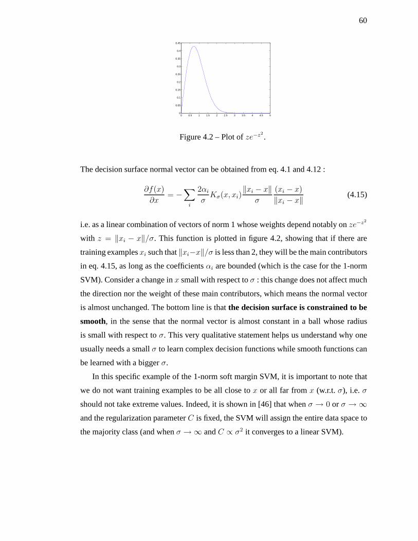
60

0 0.5 1 1.5 2 2.5 3 3.5 4 4.5 50

0.05

0.1

0.15

0.2

0.25

0.3

0.35

0.4

0.45

Figure 4.2 – Plot ofze−z2.

The decision surface normal vector can be obtained from eq. 4.1 and 4.12 :

∂f(x)

∂x= −

∑

i

2αi

σKσ(x, xi)

‖xi − x‖σ

(xi − x)

‖xi − x‖ (4.15)

i.e. as a linear combination of vectors of norm 1 whose weights depend notably onze−z2

with z = ‖xi − x‖/σ. This function is plotted in figure 4.2, showing that if thereare

training examplesxi such that‖xi−x‖/σ is less than 2, they will be the main contributors

in eq. 4.15, as long as the coefficientsαi are bounded (which is the case for the 1-norm

SVM). Consider a change inx small with respect toσ : this change does not affect much

the direction nor the weight of these main contributors, which means the normal vector

is almost unchanged. The bottom line is thatthe decision surface is constrained to be

smooth, in the sense that the normal vector is almost constant in a ball whose radius

is small with respect toσ. This very qualitative statement helps us understand why one

usually needs a smallσ to learn complex decision functions while smooth functionscan

be learned with a biggerσ.

In this specific example of the 1-norm soft margin SVM, it is important to note that

we do not want training examples to be all close tox or all far fromx (w.r.t. σ), i.e. σ

should not take extreme values. Indeed, it is shown in [46] that whenσ → 0 or σ → ∞and the regularization parameterC is fixed, the SVM will assign the entire data space to

the majority class (and whenσ → ∞ andC ∝ σ2 it converges to a linear SVM).

61

4.8 The Curse of Dimensionality for Local Non-Parametric Semi-Supervised Lear-

ning

In this section we focus on algorithms of the type described in recent papers [7,

30, 89, 90], which are graph-based non-parametric semi-supervised learning algorithms.

Because the analysis is centered on the decision surface andeq. 4.1, it also applies to

transductive SVMs and Gaussian processes when the kernel iseither Gaussian or nor-

malized Gaussian.

The graph-based algorithms we consider here can be seen as minimizing the follo-

wing cost-function, as shown in [30] :

C(Y ) = ‖Yl − Yl‖2 + µY ⊤LY + µǫ‖Y ‖2 (4.16)

with Y = (y1, . . . , yn) the estimated labels on both labeled and unlabeled data, andL the

(un-normalized) graph Laplacian derived from a similarityfunctionW between points

such thatWij = W (xi, xj) corresponds to the weights of the edges in the graph. Here,

Yl = (y1, . . . , yl) is the vector of estimated labels on thel labeled examples, whose

known labels are given byYl = (y1, . . . , yl), and one may constrainYl = Yl as in [90]

by lettingµ → 0.

Minimization of the cost criterion of eq. 4.16 can also be seen as alabel propagation

algorithm, i.e. labels are “spread” around labeled examples, with “around” being given

by the structure of the graph. An intuitive view of label propagation suggests that a

region of the manifold near a labeled (e.g. positive) example will be entirely labeled

positively, as the example spreads its influence by propagation on the graph representing

the underlying manifold. Thus, the number of regions with constant label should be on

the same order as (or less than) the number of labeled examples. This is easy to see

in the case of a sparse weight matrixW . We define a region with constant label as a

connected subset of the graph where all nodesxi have the same estimated label (sign

of yi), and such that no other node can be added while keeping theseproperties. The

following proposition then holds (note that it is also true,but trivial, whenW defines a

62

fully connected graph).

Proposition 4.8.1.After running a label propagation algorithm minimizing thecost of

eq. 4.16, the number of regions with constant estimated label is less than (or equal to)

the number of labeled examples.

Démonstration.By contradiction, if this proposition is false, then there exists a region

with constant estimated label that does not contain any labeled example. Without loss

of generality, consider the case of a positive constant label, with xl+1, . . . , xl+q the q

samples in this region. The part of the cost of eq. 4.16 depending on their labels is

C(yl+1, . . . , yl+q) =µ

2

l+q∑

i,j=l+1

Wij(yi − yj)2

+ µ

l+q∑

i=l+1

∑

j /∈l+1,...,l+qWij(yi − yj)

2

+ µǫ

l+q∑

i=l+1

y2i .

The second term is strictly positive, and because the regionwe consider is maximal (by

definition) all samplesxj outside of the region such thatWij > 0 verify yj < 0 (for xi a

sample in the region). Since allyi are stricly positive fori ∈ l+1, . . . , l+q, this means

this second term can be stricly decreased by setting allyi to 0 for i ∈ l + 1, . . . , l + q.

This also sets the first and third terms to zero (i.e. their minimum), showing that the set

of labelsyi are not optimal, which is in contradiction with their definition as the labels

that minimizeC.

This means that if the class distributions are such that there are many distinct regions

with constant labels (either separated by low-density regions or regions with samples

from the other class), we will need at least the same number oflabeled samples as there

are such regions (assuming we are using a sparse local kernelsuch as thek-nearest neigh-

bor kernel, or a thresholded Gaussian kernel). But this number couldgrow exponentially

with the dimension of the manifold(s) on which the data lie, for instance in the case of a

63

labeling function varying highly along each dimension,even if the label variations are

“simple” in a non-local sense, e.g. if they alternate in a regular fashion.

When the affinity matrixW is not sparse (e.g. Gaussian kernel), obtaining such a

result is less obvious. However, there often exists a sparseapproximation ofW (for

instance, in the case of a Gaussian kernel, one can set to 0 entries below a given threshold

or that do not correspond to ak-nearest neighbor relationship). Thus we conjecture the

same kind of result holds for dense weight matrices, if the weighting function is local in

the sense that it is close to zero when applied to a pair of examples far from each other.

4.9 General Curse of Dimensionality Argument

Can we obtain more general results that would apply to a broader class of learning

algorithms, such as transductive SVMs and Gaussian processes with Gaussian kernel ?

For this we must first establish the notion that if we choose the ballN (x) too large the

predicted function is constrained to be too smooth. The following proposition supports

this statement.

Proposition 4.9.1.For the Gaussian kernel classifier, asσ increases and becomes large

compared with the diameter of the data, in the smallest sphere containing the data the

decision surface becomes linear if∑

i αi = 0 (e.g. for SVMs), or else the normal vec-

tor of the decision surface becomes a linear combination of two sphere surface normal

vectors, with each sphere centered on a weighted average of the examples of the corres-

ponding class.

Démonstration.The decision surface is the set ofx such that

f(x) =∑

i

αie− 1

2||x−xi||2/σ2

= 0.

The normal vector of the decision surface of the Gaussian classifier is therefore

∂f(x)

∂x= −

∑

i

αi(x − xi)

σ2e−

12||x−xi||2/σ2

.

64

In the smallest sphere containing the data,||x − xi|| ≤ ∆, ∆ being the diameter of that

sphere. Asσ becomes large with respect to∆, it becomes large with respect to all the

distances||x − xi||, and the factorse−12||x−xi||2/σ2

approach1. For example forσ = 4∆,

these factors are in the interval[0.969, 1]. Let us writeβi(x) = αi

σ2 e− 1

2||x−xi||2/σ2

, which

approachesαi

σ2 . The normal vector can thus be decomposed in three terms

∂f(x)

∂x= −x

∑

i

βi(x) +∑

i:αi>0

βi(x)xi −∑

i:αi<0

(−βi(x))xi. (4.17)

Let us introduce two weighted averages, corresponding to each of the two classes. Define

for k = 1 andk = −1

Sk(x) = k∑

i:sign(αi)=k

βi(x)

mk(x) = k∑

i:sign(αi)=k

βi(x)xi

µk(x) =mk(x)

Sk(x)

These are centers of mass for each of the two classes, with weights|βi(x)|. The normal

vector is thereby written as

∂f(x)

∂x= −xS1(x) + xS−1(x) + m1(x) − m−1(x)

If∑

i αi = 0 (as in many SVMs), thenS1(x)−S−1(x) approaches 0, so that the first two

terms above vanish and the dominant remainder is the difference vectorm1−m−1, which

defines a linear decision surface whose normal vector is aligned with the difference of

two weighted means (one per class).

Without the condition∑

i αi = 0 we obtain a very specific quadratic decision sur-

face. More precisely, the normal vector can be rewritten

∂f(x)

∂x= S1(x)(µ1(x) − x) − S−1(x)(µ−1(x) − x).

65

We can now interpret the above as follows. Asσ increases,µk(x) approaches a fixed

center andSk(x) a fixed scalar, and the decision surface normal vector is a linear combi-

nation of two vectors : the normal vector of the surface of thesphere centered atµ1 and

the normal vector of the surface of the sphere centered atµ−1.

We are now ready to put all these arguments together to argue that the curse of dimen-

sionality plagues a large class of semi-supervised and supervised learning algorithms.

Conjecture 4.9.2.Consider a smoothness propertyS of discriminant functionsf . Let

P be a data-generating process from which training sets are sampled from a bounded

regionΩ. Suppose thatP is such that, withN balls coveringΩ with propertyS in each

ball, one cannot build a classifier with generalization error level less thanǫ. For kernel

machines with

1. the local-derivative property definining ballsN (x) around a given test pointx,

2. a smooth decision surface within any ballN (x) in the sense that smoothness pro-

pertyS is satisfied withinN (x) (e.g. considerS shown for the Gaussian kernel in

Proposition 4.9.1),

the number of training examples required for achieving error level ǫ grows linearly with

N . N may grow exponentially with the dimension of a manifold nearwhich the density

concentrates, on the decision surface.

Supporting argument.The notion of locality provided by thelocal-derivativeproperty

allows us to define a ballN (x) around each test pointx, containing neighbors that have

a dominating influence on∂f(x)∂x

. The smoothness propertyS defined in Proposition 4.9.1

constrains the decision surface to be either linear (case ofSVMs) or a particular quadratic

form (the decision surface normal vector is a linear combination of two vectors defined

by the center of mass of examples of each class). IfP is as defined above, one must have

at leastN balls coveringΩ, and letk be the smallest number such that one needs at least

k examples in each ball to reach error levelǫ. The number of examples thus required is

kN . To see thatN can be exponential in some dimension, consider the maximum radius

r of all these balls and the radiusR of Ω. If the region of the decision surface in which

66

the density is non-negligible has intrinsic dimensiond, thenN could be as large as the

number of radiusr balls that can tile ad-dimensional manifold of radiusR, which is at

least(

Rr

)d. This completes the argument.

4.10 Conclusion

The central claim of this paper is that there are fundamentalproblems with non-

parametric local approaches to learning, due to the curse ofdimensionality. Even though

learning algorithms such as SVMs behave better in this respect than classical algorithms

such ask-nearest-neighbor classifiers (because they can do something between thek-

nearest-neighbor and linear classifier), they also suffer from the curse of dimensionality,

at least when the kernels are local.

We have presented a series of theoretical results, some obvious and others less, that

illustrate this phenomenon. They highlight some intrinsiclimitations of those local lear-

ning algorithms, that can make them fail when applied on high-dimensional problems

where one has to look beyond what happens locally in order to overcome the curse of

dimensionality. However, there is still work to do in order to obtain more general theo-

retical results that would show precisely how the generalisation error degrades when

the (effective) dimension of the data grows, as can be done for classical non-parametric

algorithms.

Acknowledgments

The authors would like to thank the following funding organizations for support :

NSERC, MITACS, and the Canada Research Chairs. The authors are also grateful for

the feedback and stimulating exchanges that helped to shapethis paper, with Yann Le

Cun and Léon Bottou.

CHAPITRE 5

PRÉSENTATION DU DEUXIÈME ARTICLE

5.1 Détails de l’article

Convex neural networks

Y. Bengio, N. Le Roux, P. Vincent, O. Delalleau et P. Marcotte

Publié dansAdvances in Neural Information Processing Systems 18, MIT Press, Cam-

bridge, MA. en 2006.

5.2 Contexte

Le chapitre précédent a permis de mettre en lumière certaines des limitations fonda-

mentales des méthodes à noyau. Ces limitations viennent majoritairement du fait que les

caractéristiques extraites des données sont prédéfinies enfonction du noyau et qu’elles

ne sont pas apprises en tant que tel. L’apprentissage des méthodes à noyau consiste

simplement à déterminer le poids de chaque exemple d’apprentissage pour obtenir une

bonne fonction de classification.

Ces limitations encouragent naturellement à s’intéresseraux réseaux de neurones

qui apprennent les caractéristiques à extraire des données. Toutefois, la non-convexité

de leur optimisation a grandement affecté leur popularité dans la communauté de l’ap-

prentissage machine. En effet, cela a souvent été perçu comme une source potentielle

de mauvaises solutions, puisque l’entraînement ne parvenait qu’à trouver un minimum

local de la fonction de coût et pas un minimum global1.

Toutefois, l’amalgame entre localité du minimum et qualitéde la solution n’a pas

lieu d’être, comme nous allons le voir à la section suivante.

1Il existe certaines fonctions non convexes pour lesquellesla descente de gradient permet d’obtenir leminimum global, mais les fonctions de coût associées aux réseaux de neurones généraux n’en font paspartie.

68

5.2.1 Convexité

Une fonctionf deRn dansRk est convexe si et seulement si

∀x ∈ Rn, ∀y ∈ R

n, ∀λ ∈ [0, 1], f (λx + (1 − λ)y) ≤ λf(x) + (1 − λ)f(y) (5.1)

Une fonction convexe n’a qu’un seul minimum local qui est également un minimum

global. Cette propriété assure l’unicité de la solution finale obtenue par descente de gra-

dient, dispensant de la recherche d’un bon jeu de paramètresinitial.

5.2.2 Fonction de coût et optimisation

Lors de la résolution d’un problème d’apprentissage, il estsouvent impossible de

minimiser l’erreur qui nous importe réellement. Cela peut être dû à une non-dérivabilité

de cette erreur (comme dans le cas de l’erreur de classification) ou à un coût prohibitif

de son calcul (comme par exemple la vraisemblance dans une Restricted Boltzmann Ma-

chine). On utilise alors dans ce cas différentes approximations pour résoudre le problème

initial. Ces approximations peuvent être :

1. au niveau de la fonction de coût. On utilisera donc une fonction de coût simplifiée

plus facilement optimisable (c’est-à-dire dérivable, la plupart du temps)

2. au niveau de l’architecture de l’algorithme. On utilisera alors des algorithmes avec

une architecture particulière pour lesquelles le minimum de la fonction de coût est

facile à trouver (que la fonction soit convexe ou que le minimum puisse être trouvé

de façon analytique).

La qualité de la solution d’un algorithme dépend non seulement de la qualité de l’op-

timisation effectuée, mais également du judicieux de la fonction d’erreur et de l’archi-

tecture utilisées. Alors que les méthodes à noyau font le pari d’une optimisation réussie

d’une architecture simplifiée, les réseaux de neurones gardent une architecture complexe

dont le prix est une optimisation ardue.

69

5.3 Commentaires

Nous avons donc voulu montrer qu’il était possible de réaliser un algorithme possé-

dant à la fois le pouvoir de généralisation des réseaux de neurones et la simplicité d’op-

timisation des méthodes à noyau. Il en résulte un algorithmesimilaire au boosting [33]

qui sélectionne les unités cachées une par une, résolvant unproblème de classification à

chaque fois.

Ce problème de classification peut être résolu de manière exacte en temps exponen-

tiel ou de manière approchée en temps linéaire, cette accélération se faisant au prix de la

convexité. Alors que la méthode exacte réalise une meilleure performance sur l’ensemble

d’entraînement (ce qui est normal puisqu’elle atteint le minimum global), la qualité de la

solution obtenue (considérant l’erreur de test) est inférieure. Cela signifie que renoncer

à la convexité de l’optimisation peut entraîner une meilleure erreur de généralisation. Ce

résultat surprenant est analysé plus en détail par Collobert et al. [28].

CHAPITRE 6

CONVEX NEURAL NETWORKS

6.1 Abstract

Convexity has recently received a lot of attention in the machine learning commu-

nity, and the lack of convexity has been seen as a major disadvantage of many learning

algorithms, such as multi-layer artificial neural networks. We show that training multi-

layer neural networks in which the number of hidden units is learned can be viewed as

a convex optimization problem. This problem involves an infinite number of variables,

but can be solved by incrementally inserting a hidden unit ata time, each time finding a

linear classifier that minimizes a weighted sum of errors.

6.2 Introduction

The objective of this paper is not to present yet another learning algorithm, but ra-

ther to point to a previously unnoticed relation between multi-layer neural networks

(NNs),Boosting [33] and convex optimization. Its main contributions concern the ma-

thematical analysis of an algorithm that is similar to previously proposed incremental

NNs, withL1 regularization on the output weights. This analysis helps to understand the

underlying convex optimization problem that one is trying to solve.

This paper was motivated by the unproven conjecture (based on anecdotal expe-

rience) that when the number of hidden units is “large”, the resulting average error is

rather insensitive to the random initialization of the NN parameters. One way to justify

this assertion is that to really stay stuck in a local minimum, one must have second de-

rivatives positive simultaneously in all directions. Whenthe number of hidden units is

large, it seems implausible for none of them to offer a descent direction. Although this

paper does not prove or disprove the above conjecture, in trying to do so we found an in-

terestingcharacterization of the optimization problem for NNs as a convex program

if the output loss function is convex in the NN output and if the output layer weights are

71

regularized by a convex penalty. More specifically, if the regularization is theL1 norm

of the output layer weights, then we show that a “reasonable”solution exists, involving

a finite number of hidden units (no more than the number of examples, and in practice

typically much less). We present a theoretical algorithm that is reminiscent of Column

Generation [26], in which hidden neurons are inserted one ata time. Each insertion re-

quires solving a weighted classification problem, very muchlike in Boosting [33] and in

particular Gradient Boosting [34, 57].

Neural Networks, Gradient Boosting, and Column Generation

Denotex ∈ Rd+1 the extension of vectorx ∈ R

d with one element with value 1.

What we call “Neural Network” (NN) here is a predictor for supervised learning of the

form y(x) =∑m

i=1 wihi(x) wherex is an input vector,hi(x) is obtained from a linear

discriminant functionhi(x) = s(vi · x) with e.g.s(a) = sign(a), or s(a) = tanh(a) or

s(a) = 11+e−a . A learning algorithm must specify how to selectm, thewi’s and thevi’s.

The classical solution [71] involves (a) selecting a loss function Q(y, y) that specifies

how to penalize for mismatches betweeny(x) and the observedy’s (target output or

target class), (b) optionally selecting a regularization penalty that favors “small” para-

meters, and (c) choosing a method to approximately minimizethe sum of the losses on

the training dataD = (x1, y1), . . . , (xn, yn) plus the regularization penalty. Note that

in this formulation, an output non-linearity can still be used, by inserting it in the loss

functionQ. Examples of such loss functions are the quadratic loss||y − y||2, the hinge

lossmax(0, 1−yy) (used in SVMs), the cross-entropy loss−y log y− (1−y) log(1− y)

(used in logistic regression), and the exponential losse−yy (used in Boosting).

Gradient Boosting has been introduced in [34] and [57] as a non-parametric greedy-

stagewise supervised learning algorithm in which one adds afunction at a time to the

current solutiony(x), in a steepest-descent fashion, to form an additive model asabove

but with the functionshi typically taken in other kinds of sets of functions, such as those

obtained with decision trees. In a stagewise approach, whenthe(m + 1)-th basishm+1

is added, onlywm+1 is optimized (by a line search), like inmatching pursuitalgorithms.

Such a greedy-stagewise approach is also at the basis of Boosting algorithms [33], which

is usually applied using decision trees as bases andQ the exponential loss. It may be

72

difficult to minimize exactly forwm+1 andhm+1 when the previous bases and weights

are fixed, so [34] proposes to “follow the gradient” in function space, i.e., look for a

base learnerhm+1 that is best correlated with the gradient of the average losson the

y(xi) (that would be the residuey(xi)− yi in the case of the square loss). The algorithm

analyzed here also involves maximizing the correlation betweenQ′ (the derivative ofQ

with respect to its first argument, evaluated on the trainingpredictions) and the next basis

hm+1. However, we follow a “stepwise”, less greedy, approach, inwhich all the output

weights are optimized at each step, in order to obtain convergence guarantees.

Our approach adapts the Column Generation principle [26], adecomposition tech-

nique initially proposed for solving linear programs with many variables and few constraints.

In this framework, active variables, or “columns”, are onlygenerated as they are required

to decrease the objective. In several implementations, thecolumn-generation subproblem

is frequently a combinatorial problem for which efficient algorithms are available. In our

case, the subproblem corresponds to determining an “optimal” linear classifier.

6.3 Core Ideas

Informally, consider the setH of all possible hidden unit functions (i.e., of all pos-

sible hidden unit weight vectorsvi). Imagine a NN that has all the elements in this set as

hidden units. We might want to impose precision limitationson those weights to obtain

either a countable or even a finite set. For such a NN, we only need to learn the output

weights. If we end up with a finite number of non-zero output weights, we will have

at the end an ordinary feedforward NN. This can be achieved byusing a regularization

penalty on the output weights that yields sparse solutions,such as theL1 penalty. If in

addition the loss function is convex in the output layer weights (which is the case of

squared error, hinge loss,ǫ-tube regression loss, and logistic or softmax cross-entropy),

then it is easy to show that the overall training criterion isconvex in the parameters

(which are now only the output weights). The only problem is that there are as many

variables in this convex program as there are elements in thesetH, which may be very

large (possibly infinite). However, we find that withL1 regularization, a finite solution is

73

obtained, and that such a solution can be obtained by greedily inserting one hidden unit

at a time. Furthermore, it is theoretically possible to check that the global optimum has

been reached.

Definition 6.3.1. LetH be a set of functions from an input spaceX to R. Elements ofHcan be understood as “hidden units” in a NN. LetW be the Hilbert space of functions

fromH to R, with an inner product denoted bya · b for a, b ∈ W. An element ofW can

be understood as the output weights vector in a neural network. Leth(x) : H → R the

function that maps any elementhi ofH to hi(x). h(x) can be understood as the vector of

activations of hidden units when inputx is observed. Letw ∈ W represent aparameter

(the output weights). The NN prediction is denotedy(x) = w ·h(x). LetQ : R×R → R

be a cost function convex in its first argument that takes a scalar prediction y(x) and

a scalar target valuey and returns a scalar cost. This is the cost to be minimized on

example pair(x, y). Let D = (xi, yi) : 1 ≤ i ≤ n a training set. LetΩ : W → R

be a convex regularization functional that penalizes for the choice of more “complex”

parameters (e.g.,Ω(w) = λ||w||1 according to a 1-norm inW, if H is countable). We

define theconvex NN criterionC(H, Q, Ω, D, w) with parameterw as follows :

C(H, Q, Ω, D, w) = Ω(w) +n∑

t=1

Q(w · h(xt), yt). (6.1)

The following is a trivial lemma, but it is conceptually veryimportant as it is the

basis for the rest of the analysis in this paper.

Lemma 6.3.2.The convex NN costC(H, Q, Ω, D, w) is a convex function ofw.

Démonstration.Q(w · h(xt), yt) is convex inw andΩ is convex inw, by the above

construction.C is additive inQ(w · h(xt), yt) and additive inΩ. HenceC is convex in

w.

Note that there are no constraints in this convex optimization program, so that at the

global minimum all the partial derivatives ofC with respect to elements ofw cancel.

Let |H| be the cardinality of the setH. If it is not finite, it is not obvious that an

optimal solution can be achieved in finitely many iterations.

74

Lemma 6.3.2 says that training NNs from a very large class (with one or more hidden

layer) can be seen as convex optimization problems, usuallyin a very high dimensional

space,as long as we allow the number of hidden units to be selected bythe learning

algorithm . By choosing a regularizer that promotessparsesolutions, we obtain a so-

lution that has afinite number of “active” hidden units (non-zero entries in the output

weights vectorw). This assertion is proven below, in theorem 6.4.1, for the case of the

hinge loss.

However, even if the solution involves a finite number of active hidden units, the

convex optimization problem could still be computationally intractable because of the

large number of variables involved. One approach to this problem is to apply the prin-

ciples already successfully embedded in Gradient Boosting, but more specifically in Co-

lumn Generation (an optimization technique for very large scale linear programs), i.e.,

add one hidden unit at a time in an incremental fashion. Theimportant ingredient here

is a way to know that we have reached the global optimum, thus not requiring to

actually visit all the possible hidden units.We show that this can be achieved as long

as we can solve the sub-problem of finding a linear classifier that minimizes the weighted

sum of classification errors. This can be done exactly only onlow dimensional data sets

but can be well approached using weighted linear SVMs, weighted logistic regression,

or Perceptron-type algorithms.

Another idea (not followed up here) would be to consider firsta smaller setH1,

for which the convex problem can be solved in polynomial time, and whose solution can

theoretically be selected as initialization for minimizing the criterionC(H2, Q, Ω, D, w),

with H1 ⊂ H2, and whereH2 may have infinite cardinality (countable or not). In this

way we could show that we can find a solution whose cost satisfiesC(H2, Q, Ω, D, w) ≤C(H1, Q, Ω, D, w), i.e., is at least as good as the solution of a more restrictedconvex

optimization problem. The second minimization can be performed with a local descent

algorithm, without the necessity to guarantee that the global optimum will be found.

75

6.4 Finite Number of Hidden Neurons

In this section we consider the special case withQ(y, y) = max(0, 1−yy) the hinge

loss, andL1 regularization, and we show that the global optimum of the convex cost

involves at mostn + 1 hidden neurons, using an approach already exploited in [67]for

L1-loss regression Boosting withL1 regularization of output weights.

The training criterion isC(w) = K‖w‖1 +n∑

t=1

max (0, 1 − ytw · h(xt)). Let us re-

write this cost function as the constrained optimization problem :

minw,ξ

L(w, ξ) = K‖w‖1 +n∑

t=1

ξt s.t.

yt [w · h(xt)] ≥ 1 − ξt (C1)

and ξt ≥ 0, t = 1, . . . , n (C2)

Using a standard technique, the above program can be recast as a linear program.

Definingλ = (λ1, . . . , λn) the vector of Lagrangian multipliers for the constraintsC1,

its dual problem(P ) takes the form (in the case of a finite numberJ of base learners) :

(P ) : maxλ

n∑

t=1

λt s.t.

λ · Zi − K ≤ 0, i ∈ I

and λt ≤ 1, t = 1, . . . , n

with (Zi)t = ythi(xt). In the case of a finite numberJ of base learners,I = 1, . . . , J.

If the number of hidden units is uncountable, thenI is a closed bounded interval ofR.

Such an optimization problem satisfies all the conditions needed for using Theorem

4.2 from [38]. Indeed :

• I is compact (as a closed bounded interval ofR) ;

• F : λ 7→∑nt=1 λt is a concave function (it is even a linear function) ;

• g : (λ, i) 7→ λ · Zi − K is convex inλ (it is actually linear inλ) ;

• ν(P ) ≤ n (therefore finite) (ν(P ) is the largest value ofF satisfying the constraints) ;

• for every set ofn + 1 pointsi0, . . . , in ∈ I, there existsλ such thatg(λ, ij) < 0 for

j = 0, . . . , n (one can takeλ = 0 sinceK > 0).

Then, from Theorem 4.2 from [38], the following theorem holds :

Theorem 6.4.1.The solution of(P ) can be attained with alternate constraintsC ′2 and

76

only n + 1 constraintsC ′1 (i.e., there exists a subset ofn + 1 constraintsC ′

1 giving

rise to the same maximum as when using the whole set of constraints). Even though

these constraints are unknown, this ensures that the primalproblem associated is the

minimization of the cost function of a NN withn + 1 hidden neurons.

6.5 Incremental Convex NN Algorithm

In this section we present a stepwise algorithm to optimize aNN, and show that there

is a criterion that allows to verify whether the global optimum has been reached. This is

a specialization of minimizingC(H, Q, Ω, D, w), with Ω(w) = λ||w||1 andH = h :

h(x) = s(v · x) is the set of soft or hard linear classifiers (depending on choice ofs(·)).

77

Algorithm ConvexNN(D,Q,λ,s)

Input : training setD = (x1, y1), . . . , (xn, yn), convex loss functionQ, and

scalar regularization penaltyλ. s is either thesignfunction or thetanhfunction.

(1) Setv1 = (0, 0, . . . , 1) and selectw1 = argminw

∑t Q(ws(1), yt) + λ|w|.

(2) Seti = 2.

(3) Repeat

(4) Let qt = Q′(∑i−1

j=1 wjhj(xt), yt)

(5) If s = sign

(5a) train linear classifierhi(x) = sign(vi · x) with examples(xt, sign(qt))and errors weighted by|qt|, t = 1 . . . n (i.e.,maximize

∑t qthi(xt))

(5b) else (s = tanh)

(5c) train linear classifierhi(x) = tanh(vi · x) to maximize∑

t qthi(xt).

(6) If∑

t qthi(xt) < λ, stop.

(7) Selectw1, . . . , wi (and optionallyv2, . . . , vi) minimizing (exactly or

approximately)C =∑

t Q(∑i

j=1 wjhj(xt), yt) + λ∑

j=1 |wj|such that∂C

∂wj= 0 for j = 1 . . . i.

(7) Incrementi by 1.

(9) Return the predictory(x) =∑i

j=1 wjhj(x).

A key property of the above algorithm is that, at termination, the global optimum is

reached, i.e., no hidden unit (linear classifier) can improve the objective. In the case

wheres = sign, we obtain a Boosting-like algorithm, i.e., it involves finding a classifier

which minimizes the weighted cost∑

t qtsign(v · xt).

Theorem 6.5.1.AlgorithmConvexNNstops when it reaches the global optimum of

C(w) =∑

t Q(w · h(xt), yt) + λ||w||1.

Démonstration.Let w be the output weights vector when the algorithm stops. Because

the set of hidden unitsH we consider is such that whenh is in H, −h is also inH, we

can assume all weights to be non-negative. By contradiction, if w′ 6= w is the global

78

optimum, withC(w′) < C(w), then, sinceC is convex in the output weights, for any

ǫ ∈ (0, 1), we haveC(ǫw′ + (1 − ǫ)w) ≤ ǫC(w′) + (1 − ǫ)C(w) < C(w). Let wǫ =

ǫw′ + (1 − ǫ)w. For ǫ small enough, we can assume all weights inw that are strictly

positive to be also strictly positive inwǫ. Let us denote byIp the set of strictly positive

weights inw (andwǫ), by Iz the set of weights set to zero inw but to a non-zero value

in wǫ, and byδǫk the differencewǫ,k −wk in the weight of hidden unithk betweenw and

wǫ. We can assumeδǫj < 0 for j ∈ Iz, because instead of setting a small positive weight

to hj , one can decrease the weight of−hj by the same amount, which will give either the

same cost, or possibly a lower one when the weight of−hj is positive. Witho(ǫ) denoting

a quantity such thatǫ−1o(ǫ) → 0 whenǫ → 0, the difference∆ǫ(w) = C(wǫ) − C(w)

can now be written :

∆ǫ(w) = λ (‖wǫ‖1 − ‖w‖1) +∑

t

(Q(wǫ · h(xt), yt) − Q(w · h(xt), yt))

= λ

∑

i∈Ip

δǫi +∑

j∈Iz

−δǫj

+

∑

t

∑

k

(Q′(w · h(xt), yt)δǫkhk(xt)) + o(ǫ)

=∑

i∈Ip

(λδǫi +

∑

t

qtδǫihi(xt)

)+∑

j∈Iz

(−λδǫj +

∑

t

qtδǫjhj(xt)

)+ o(ǫ)

=∑

i∈Ip

δǫi∂C

∂wi(w) +

∑

j∈Iz

(−λδǫj +

∑

t

qtδǫjhj(xt)

)+ o(ǫ)

= 0 +∑

j∈Iz

(−λδǫj +

∑

t

qtδǫjhj(xt)

)+ o(ǫ)

since fori ∈ Ip, thanks to step(7) of the algorithm, we have∂C∂wi

(w) = 0. Thus the

inequalityǫ−1∆ǫ(w) < 0 rewrites into

∑

j∈Iz

ǫ−1δǫj

(−λ +

∑

t

qthj(xt)

)+ ǫ−1o(ǫ) < 0

which, whenǫ → 0, yields (note thatǫ−1δǫj does not depend onǫ sinceδǫj is linear in

79

ǫ) :∑

j∈Iz

ǫ−1δǫj

(−λ +

∑

t

qthj(xt)

)≤ 0 (6.2)

But, hi being the optimal classifier chosen in step (5a) or (5c), all hidden unitshj verify∑

t qthj(xt) ≤ ∑t qthi(xt) < λ and∀j ∈ Iz, ǫ−1δǫj (−λ +

∑t qthj(xt)) > 0 (since

δǫj < 0), contradicting eq. 6.2.

[57] prove a related global convergence result for the AnyBoost algorithm, a non-

parametric Boosting algorithm that is also similar to Gradient Boosting [34]. Again,

this requires solving as a sub-problem an exact minimization to find a functionhi ∈ Hthat is maximally correlated with the gradientQ′ on the output. We now show a simple

procedure to select a hyperplane with the best weighted classification error.

Exact Minimization

In step (5a) we are required to find a linear classifier that minimizes the weighted sum

of classification errors. Unfortunately, this is an NP-hardproblem (w.r.t.d, see theorem

4 in [56]). However, an exact solution can be easily found inO(n3) computations for

d = 2 inputs.

Proposition 6.5.2.Finding a linear classifier that minimizes the weighted sum of clas-

sification error can be achieved inO(n3) steps when the input dimension isd = 2.

Démonstration.We want to maximize∑

i cisign(u · xi + b) with respect tou andb, the

ci’s being inR. Consideru fixed and sort thexi’s according to their dot product with

u and denoter the function which mapsi to r(i) such thatxr(i) is in i-th position in

the sort. Depending on the value ofb, we will haven + 1 possible sums, respectively

−∑ki=1 cr(i) +

∑ni=k+1 cr(i), k = 0, . . . , n. It is obvious that those sums only depend on

the order of the productsu · xi, i = 1, . . . , n. Whenu varies smoothly on the unit circle,

as the dot product is a continuous function of its arguments,the changes in the order

of the dot products will occur only when there is a pair(i, j) such thatu · xi = u · xj .

Therefore, there are at most as many order changes as there are pairs of different points,

i.e.,n(n−1)/2. In the case ofd = 2, we can enumerate all the different angles for which

there is a change, namelya1, . . . , az with z ≤ n(n−1)2

. We then need to test at least one

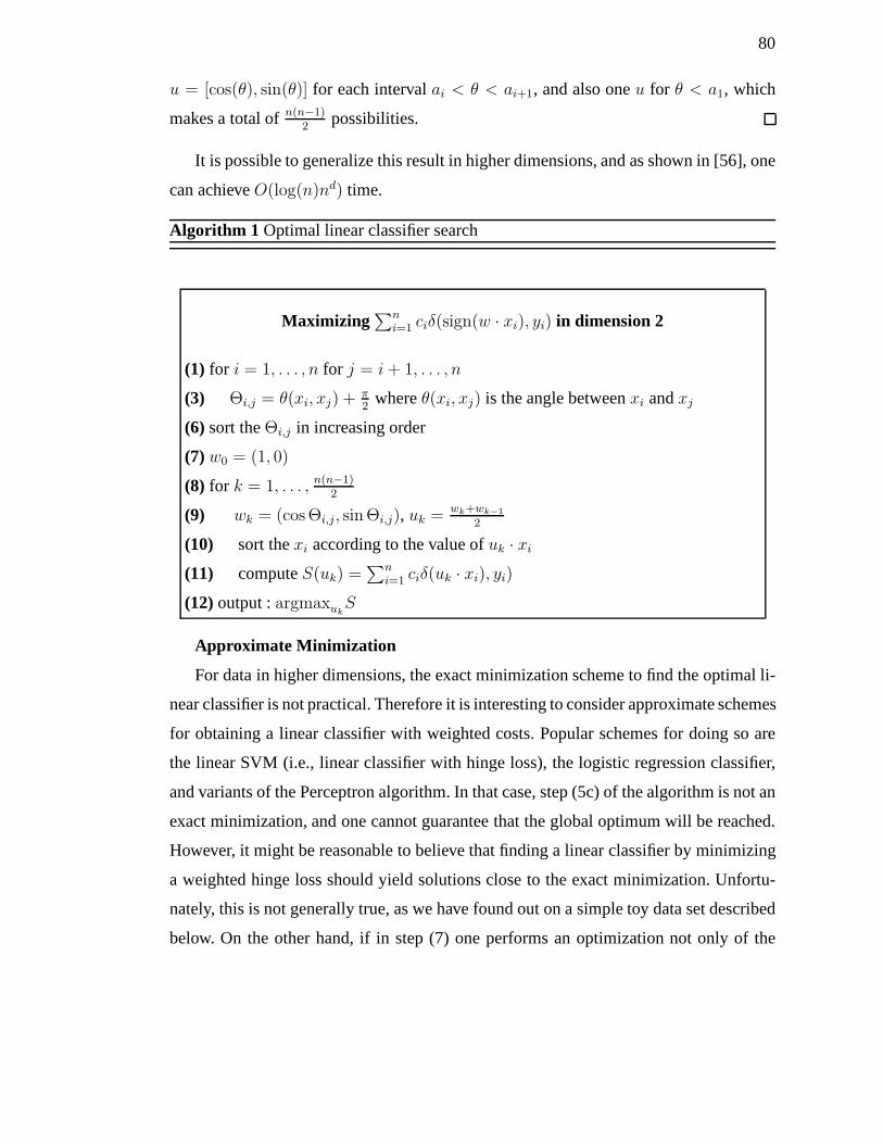
80

u = [cos(θ), sin(θ)] for each intervalai < θ < ai+1, and also oneu for θ < a1, which

makes a total ofn(n−1)2

possibilities.

It is possible to generalize this result in higher dimensions, and as shown in [56], one

can achieveO(log(n)nd) time.

Algorithm 1 Optimal linear classifier search

Maximizing∑n

i=1 ciδ(sign(w · xi), yi) in dimension 2

(1) for i = 1, . . . , n for j = i + 1, . . . , n

(3) Θi,j = θ(xi, xj) + π2

whereθ(xi, xj) is the angle betweenxi andxj

(6) sort theΘi,j in increasing order

(7) w0 = (1, 0)

(8) for k = 1, . . . , n(n−1)2

(9) wk = (cos Θi,j, sin Θi,j), uk = wk+wk−1

2

(10) sort thexi according to the value ofuk · xi

(11) computeS(uk) =∑n

i=1 ciδ(uk · xi), yi)

(12)output :argmaxukS

Approximate Minimization

For data in higher dimensions, the exact minimization scheme to find the optimal li-

near classifier is not practical. Therefore it is interesting to consider approximate schemes

for obtaining a linear classifier with weighted costs. Popular schemes for doing so are

the linear SVM (i.e., linear classifier with hinge loss), thelogistic regression classifier,

and variants of the Perceptron algorithm. In that case, step(5c) of the algorithm is not an

exact minimization, and one cannot guarantee that the global optimum will be reached.

However, it might be reasonable to believe that finding a linear classifier by minimizing

a weighted hinge loss should yield solutions close to the exact minimization. Unfortu-

nately, this is not generally true, as we have found out on a simple toy data set described

below. On the other hand, if in step (7) one performs an optimization not only of the

81

output weightswj (j ≤ i) but also of the corresponding weight vectorsvj , then the algo-

rithm finds a solution close to the global optimum (we could only verify this on 2D data

sets, where the exact solution can be computed easily). It means that at the end of each

stage, one first performs a few training iterations of the whole NN (for the hidden units

j ≤ i) with an ordinary gradient descent mechanism (we used conjugate gradients but

stochastic gradient descent would work too), optimizing the wj ’s and thevj ’s, and then

one fixes thevj ’s and obtains the optimalwj ’s for thesevj ’s (using a convex optimization

procedure). In our experiments we used a quadraticQ, for which the optimization of the

output weights can be done with a neural network, using the outputs of the hidden layer

as inputs.

Let us consider now a bit more carefully what it means to tune thevj ’s in step (7).

Indeed, changing the weight vectorvj of a selected hidden neuron to decrease the cost

is equivalent to a change in the output weightsw’s. More precisely, consider the step

in which the value ofvj becomesv′j. This is equivalent to the following operation on the

w’s, whenwj is the corresponding output weight value : the output weightassociated

with the valuevj of a hidden neuron is set to 0, and the output weight associated with

the valuev′j of a hidden neuron is set towj. This corresponds to an exchange between

two variables in the convex program. We are justified to take any such step as long as it

allows us to decrease the costC(w). The fact that we are simultaneously making such

exchanges on all the hidden units when we tune thevj ’s allows us to move faster towards

the global optimum.

Extension to multiple outputs

The multiple outputs case is more involved than the single-output case because it is

not enough to check the condition∑

t htqt > λ. Consider a new hidden neuron whose

output ishi when the input isxi. Let us also denoteα = [α1, . . . , αno]′ the vector of

output weights between the new hidden neuron and theno output neurons. The gradient

with respect toαj isgj = ∂C∂αj

=∑

t htqtj−λsign(αj) with qtj the value of the j-th output

neuron with inputxt. This means that if, for a givenj, we have|∑t htqtj | < λ, moving

αj away from 0 can only increase the cost. Therefore, the right quantity to consider is

(|∑t htqtj | − λ)+.

82

We must therefore findargmaxv

∑j (|∑t htqtj | − λ)2

+. As before, this sub-problem

is not convex, but it is not as obvious how to approximate it bya convex problem. The

stopping criterion becomes : if there is noj such that|∑t htqtj | > λ, then all weights

must remain equal to 0 and a global minimum is reached.

Experimental Results

We performed experiments on the 2D double moon toy dataset (as used in [31]),

to be able to compare with the exact version of the algorithm.In these experiments,

Q(w · h(xt), yt) = [w · h(xt) − yt]2. The set-up is the following :

• Select a new linear classifier, either (a) the optimal one or (b) an approximate using

logistic regression.

• Optimize the output weights using a convex optimizer.

• In case (b), tune both input and output weights by conjugate gradient descent onC and

finally re-optimize the output weights using LASSO regression.

• Optionally, remove neurons whose output weight has been setto 0.

Using the approximate algorithm yielded for 100 training examples an average pe-

nalized (λ = 1) squared error of 17.11 (over 10 runs), an average test classification error

of 3.68% and an average number of neurons of 5.5. The exact algorithm yielded a pena-

lized squared error of 8.09, an average test classification error of 5.3%, and required 3

hidden neurons. A penalty ofλ = 1 was nearly optimal for the exact algorithm whereas

a smaller penalty further improved the test classification error of the approximate algo-

rithm. Besides, when running the approximate algorithm fora long time, it converges to

a solution whose quadratic error is extremely close to the one of the exact algorithm.

6.6 Conclusion

We have shown that training a NN can be seen as a convex optimization problem,

and have analyzed an algorithm that can exactly or approximately solve this problem.

We have shown that the solution with the hinge loss involved anumber of non-zero

weights bounded by the number of examples, and much smaller in practice. We have

shown that there exists a stopping criterion to verify if theglobal optimum has been

83

reached, but it involves solving a sub-learning problem involving a linear classifier with

weighted errors, which can be computationally hard if the exact solution is sought, but

can be easily implemented for toy data sets (in low dimension), for comparing exact and

approximate solutions.

The above experimental results are in agreement with our initial conjecture : when

there are many hidden units we are much less likely to stall inthe optimization procedure,

because there are many more ways to descend on the convex costC(w). They also

suggest, based on experiments in which we can compare with the exact sub-problem

minimization, that applying AlgorithmConvexNN with an approximate minimization

for adding each hidden unitwhile continuing to tune the previous hidden unitstends

to lead to fast convergence to the global minimum. What can get us stuck in a “local

minimum” (in the traditional sense, i.e., of optimizingw’s andv’s together) is simply

the inability to find a new hidden unit weight vector that can improve the total cost

(fit and regularization term) even if there exists one.

Note that as a side-effect of the results presented here, we have a simple way to train

neural networks with hard-threshold hidden units, since increasing∑

t Q′(y(xt), yt)sign(vixt)

can be either achieved exactly (at great price) or approximately (e.g. by using a cross-

entropy or hinge loss on the corresponding linear classifier).

Acknowledgments

The authors thank the following for support : NSERC, MITACS,and the Canada

Research Chairs. They are also grateful for the feedback andstimulating exchanges with

Sam Roweis, Nathan Srebro, and Aaron Courville.

CHAPITRE 7

PRÉSENTATION DU TROISIÈME ARTICLE

7.1 Détails de l’article

Continuous Neural Networks

N. Le Roux et Y. Bengio

Publié dansProceedings of the Eleventh International Workshop on Artificial Intelli-

gence and Statisticsen 2007.

7.2 Contexte

Les réseaux convexes présentés au chapitre précédent ouvrirent la voie des réseaux

infinis en conservant une solution finale exprimable avec un nombre fini de paramètres.

Toutefois, comme nous avons pu le voir, leur optimisation requiert un temps exponentiel

et ils généralisaient parfois moins bien que leur version approchée.

L’article ci-après a pour but de proposer une nouvelle vision des réseaux de neurones

donnant naissance à des réseaux de neurones infinis dont l’optimisation est aussi rapide

que pour des réseaux normaux. Il renforce également le lien,déjà étudié par Neal [60]

et Williams [83], entre les réseaux de neurones et les méthodes à noyau.

7.3 Commentaires

L’idée sous-jacente de l’article est qu’un réseau de neurones à une couche cachée

modélise une primitive d’une fonction constante par morceaux, chaque unité cachée

correspondant à un morceau différent. Lorsque le nombre d’unités cachées tend vers

l’infini, le nombre de morceaux fait de même et le réseau de neurones modélise la pri-

mitive d’une fonction quelconque. L’apprentissage d’un réseau de neurones peut donc

être vu comme l’approximation d’une fonction quelconque (la fonction dont on calcule

85

la primitive) par une fonction constante par morceaux.

Les réseaux continus, de leur côté, tentent d’approcher cette fonction par une fonc-

tion affine par morceaux. Cette modélisation est strictement plus puissante que les ré-

seaux de neurones standards (en ce sens qu’il existe des réseaux continus qu’il est im-

possible de modéliser avec des réseaux standards alors que l’inverse est faux).

Les réseaux continus se sont effectivement avérés plus puissants que les réseaux de

neurones standards sur certaines tâches, mais les résultats furent décevants sur d’autres.

L’une des raisons possibles est la difficulté de l’optimisation induite par une telle pa-

ramétrisation. En effet, bien que le nombre de paramètres reste raisonnable, les unités

cachées deviennent liées les unes aux autres, entraînant des dépendances complexes pré-

judiciables à la descente de gradient.

De son côté, le noyau induit par les réseaux infinis utilisantla fonction de Heaviside

comme fonction de transfert est intéressant, tant par sa simplicité que par la qualité des

résultats qu’il occasionne. Il n’est pas non plus inutile deremarquer que ce noyau n’est

pas local, au contraire du noyau gaussien.

CHAPITRE 8

CONTINUOUS NEURAL NETWORKS

8.1 Abstract

This article extends neural networks to the case of an uncountable number of hidden

units, in several ways. In the first approach proposed, a finite parametrization is possible,

allowing gradient-based learning. For the same number of parameters than an ordinary

neural network, this model yields lower error on real-worlddata while having a lower ca-

pacity. Better error bounds than with ordinary neural networks are shown using an affine

parametrization of the input-to-hidden weights. Experimental results show that optimi-

zation is easier than with ordinary neural networks, possibly by reducing the problem

of hidden unit saturation. In a second approach the input-to-hidden weights are fully

non-parametric, yielding a kernel machine for which we demonstrate a simple kernel

formula. Interestingly, the resulting kernel machine can be made hyperparameter-free,

and still generalizes in spite of an absence of explicit regularization.

8.2 Introduction

In [60] neural networks with an infinite number of hidden units were introduced,

showing that they could be interpreted as Gaussian processes, and this work served

as inspiration for a large body of work on Gaussian processes. Neal’s work showed a

counter-example to two common beliefs in the machine learning community : (1) that

a neural network with a very large number of hidden units would overfit and (2) that it

would not be feasible to numerically optimize such huge networks. In spite of Neal’s

work, these beliefs are still commonly held. In this paper wereturn to Neal’s idea and

study a number of extensions of neural networks to the case where the number of hidden

units is uncountable, and show that they yield implementable algorithms with interesting

properties.

Consider a neural network with one hidden layer (andh hidden neurons), one output

87

neuron and a transfer functiong. Let us denoteV the input-to-hidden weights,ai(i =

1, . . . , h) the hidden-to-output weights andβ the output unit bias (the hidden units bias

is included inV ).

The output of the network with inputx is then

f(x) = β +∑

i

aig(x · Vi) (8.1)

whereVi is theith column of matrixV and x is the vector with1 appended tox. The

output of theith hidden neuron isg(x · Vi). For symmetric functionsg such astanh, we

can without any restriction consider the case where all theai’s are nonnegative, since

changing the sign ofai is equivalent to changing the sign ofVi.

In ordinary neural networks we have an integer indexi. To obtain an uncountable

number of hidden units, we introduce a continuous-valued (possibly vector-valued) in-

dexz ∈ Rm, with m ≤ d + 1. We can replace the usual sum over hidden units by an

integral that goes through the different weight vectors that can be assigned to a hidden

unit :

f(x) = β +

∫a(z)g[x · V (z)] dz (8.2)

wherea : Rm → R is the hidden-to-output weight function, andV : R

m → Rd+1 is the

input-to-hidden weight function. Alternatively, function a can be replaced by a single

scalarα wheng is invertible over some range. Leta(z) = αγ(z) whereα is a global

constant such thatγ(z)g(x·V (z)) is in the domain ofg for all z. Then one can find a func-

tion b(z) such thata(z)g(x · V (z)) = αg(b(z)x · V (z)), i.e.b(z) = g−1(a(z)g(x·(V (z)))/α)x·V (z)

,

andV (z) can be replaced byb(z)V (z). An equivalent parametrization is therefore

f(x) = α

∫g[x · V (z)] dz. (8.3)

How can we prevent overfitting in these settings ? In this paper we discuss three types

of solutions : (1) finite-dimensional representations ofV (using formulation 8.3). (2)L1

regularization of the output weights witha andV completely free (3)L2 regularization

of the output weights, witha andV completely free.

88

Solutions of type 1 are completely new and surprising results are obtained with them.

Many possible parametrizations are possible to map the “hidden unit index” (a finite-

dimensional vector) to a weight vector. This parametrization allows to show a represen-

tation theorem similar to Kolmogorov’s, i.e. we show that functions fromRd to R can be

represented byd + 1 functions fromR to R. Here we study an affine-by-part parametri-

zation, with interesting properties. In particular, it is shown that approximation error can

be bounded inO(h−2) whereh is proportional to the number of free parameters, whereas

ordinary neural networks enjoy aO(h−1) error bound. Experiments suggest that optimi-

zing them is easier than optimizing ordinary neural networks, probably because they are

less sensitive to the saturation problem (when the weightedsum of a hidden unit is large,

the derivative through it is close to 0, making it difficult tooptimize the input-to-hidden

weights of that hidden unit). Solutions of type 2 (L1 regularization) were already presen-

ted in [16] so we do not focus on them here. They also yield to a convex formulation but

in an infinite number of variables, requiring approximate optimization. Solutions of type

3 (L2 regularization) give rise to kernel machines that are similar to Gaussian processes,

albeit with a type of kernel not commonly used in the litterature. We show that an ana-

lytic formulation of the kernel is possible when hidden units compute the sign of a dot

product (i.e., with formal neurons). Interestingly, experiments suggest that this kernel is

more resistant to overfitting than the Gaussian kernel, allowing to train working models

without a single hyper-parameter.

8.3 Affine neural networks

8.3.1 Core idea

We study here a special case of the solutions of type (1), witha finite-dimensional pa-

rametrization of the continuous neural network, based on parametrizingV (z) in eq. 8.3,

wherez is scalar. In this case, without loss of generality we can take the domain ofz to

be the unit interval, thus

f(x) = β + α

∫ 1

0

g[x · V (z)] dz (8.4)

89

whereV is a function fromR to Rd+1 (d being the dimension ofx).

It is easy to see that this becomes formula (8.1) whenV is a piecewise-constant

function such that

V (z) = Vi when pi−1 ≤ z < pi

with a0 = 0, α =∑

i ai andpi = 1α

∑ij=0 aj .

At this point, we can make an important comment. Ifx ∈ Rd we can rewritex ·

V (z) = V d+1(z) +∑d

i=1 xiVi(z) whereV i is a function fromR to R andxi is the

i-th coordinate ofx for eachi. But f is a function fromRd to R. Using neural network

function approximation theorems, the following theorem therefore follows :

Theorem 8.3.1.Any functionf fromRd to R can, with an arbitrary precision, be defined

byd + 1 functionsV i fromR to R and two realsα andβ with the relation

f(x) = β + α

∫ 1

0

tanh

(d∑

i=1

V i(z) · xi + V n+1(z)

)dz

This result is reminiscent of Kolmogorov’s superposition theorem [48], but here we

show that the functionsV i can be directly optimized in order to obtain a good function

approximation.

8.3.2 Approximating an Integral

The formulation in eq. 8.4 shows that the only thing to optimize will be the func-

tion V , and the scalarsα andβ, getting rid of the optimization of the hidden-to-output

weights.

In this work we consider a parametrization ofV involving a finite number of para-

meters, and we optimize over these parameters. Sincef is linked toV by an integral,

it suggests to look over parametrizations yielding good approximation of an integral.

Several such parametrizations already exist :

– piecewise constant functions, used in the rectangle method. This is the simplest

approximation, corresponding to ordinary neural networks(eq. 8.1),

90

– piecewise affine functions, used in the trapezoid method. This approximation yields

better results and will be the one studied here, which we coin“Affine Neural Net-

work”.

– polynomials, used in Simpson’s method, which allow even faster convergence.

However, we were not able to compute the integral of polynomials through the

functiontanh.

8.3.3 Piecewise Affine Parametrization

Using a piecewise affine parametrization, we considerV of the form :

V (z) = Vi−1 +z − pi−1

pi − pi−1(Vi − Vi−1) whenpi−1 ≤ z < pi,

that is to sayV is linear betweenpi−1 andpi, V (pi−1) = Vi−1 andV (pi) = Vi for eachi.

This will ensure the continuity ofV .

Besides, we will setVn+1 = V1 to avoid border effects and obtain an extra segment

for the same number of parameters.

Rewritingpi = pi−1 = ai andV (z) = Vi(z) whenpi−1 ≤ z < pi, the output for an

input examplex can be written :

f(x) =∑

i

∫ pi

z=pi−1

tanh [Vi(z) · x]

f(x) =∑

i

ai

(Vi − Vi−1) · xln

(cosh(Vi · x)

cosh(Vi−1 · x)

)(8.5)

To respect the continuity of the functionV , we should restrict theai to be positive since

pi must be greater thanpi−1. However, in our experiments, we did not use that restric-

tion to simplify gradient descent over the parameters. We believe that this makes little

difference in the final result.

91

8.3.3.1 Is the continuity ofV necessary ?

As said before, we want to enforce the continuity ofV . The first reason is that the

trapezoid method uses continuous functions and the resultsconcerning that method can

therefore be used for our approximation. Besides, we have this intuition that a “reasona-

ble” functionf will use a “reasonable” functionV . This intuition will not be theoretically

verified here but it seems to be validated by the experimentalresults.

The reader might notice at that point that there is no bijection betweenV andf .

Indeed, sinceV is only defined by its integral, we can switch two different pieces of

V without modifyingf . Thus, it would more correct to say that iff is a “reasonable”

function, then there must exist a “reasonable”V that gives rise tof .

8.3.4 Extension to multiple output neurons

The formula of the output is a linear combination of theai, as in the ordinary neural

network. Thus, the extension tol output neurons is straightforward using the formula

fj(x) =∑

i

aij

(Vi − Vi−1) · xln

(cosh(Vi · x)

cosh(Vi−1 · x)

)(8.6)

for j = 1, . . . , l.

8.3.5 Piecewise affine versus piecewise constant

Consider a target functionf ∗ that we would like to approximate, and a targetV ∗ that

gives rise to it. Before going any further, we should ask ourselves two questions :

– is there a relation between the quality of the approximation of f ∗ and the quality

of approximation ofV ∗ ?

– are piecewise affine functions (i.e. our affine neural networks) more appropriate to

approximate an arbitrary function than the piecewise constant ones (i.e. ordinary

neural networks) ?

92

8.3.5.1 Relation betweenf and V

To answer the first of those questions, we will bound the errorbetweenf(x) and

f ∗(x) using the error betweenV andV ∗. First assume thatα = α∗ andβ = β∗.

|f(x) − f ∗(x)| =

= a∗∣∣∣∣∫

z

(tanh [V (z) · x] − tanh [V ∗(z) · x]) dz

∣∣∣∣

= a∗ |∫

z

tanh [(V (z) − V ∗(z)) · x]

(1 − tanh [V (z) · x] tanh [V ∗(z) · x]) dz|≤ a∗

∫

z

|tanh [(V (z) − V ∗(z)) · x]| dz

× supz

|1 − tanh [V (z) · x] tanh [V ∗(z) · x]|

≤ 2a∗∫

z

|tanh [(V (z) − V ∗(z)) · x]| dz

≤ 2a∗∫

z

tanh [|(V (z) − V ∗(z)) · x|] dz

But for a givenV , the difference betweenf andf ∗ can only be smaller if we allow

(α, β) to be different from(α∗, b∗) (i.e. choosingα andβ optimally). Therefore, the

inequality remains whenα andβ are not fixed.

The difference between the approximate functionf usingV and the true functionf ∗

is therefore bounded by2α∗ ∫ztanh [|(V (z) − V ∗(z)) · x|] dz, which is itself bounded

by 2α∗ × supz tanh [|(V ∗ − V )(z) · x|].Thus, ifV is never far fromV ∗, we are sure that the approximated function will be

close from the true function. This makes reasonable our try to better approximateV ∗.

We can then make an obvious remark : if we restrict ourselves to a finite number of

hidden neurons, it will never be possible to have a piecewiseconstant function equal to a

piecewise affine function (apart from the trivial case whereall affine functions are in fact

constant). On the other hand, any piecewise contant function composed ofh pieces can

be represented arbitrarily closely by a continuous piecewise affine function composed

of at most2h pieces (half of the pieces being constant and the other half being used to

93

avoid discontinuities).

A second remark can be made : for any piecewise constant function and any conti-

nuous piecewise affine function, given that they are not equal, one can find a function

that is better approximated by the first class than by the second class ; it is trivial to see

that one can also find a function that is better approximated by the second class than by

the first class.

After those trivial comments, let us focus on less evident remarks. As shown in sec-

tion 8.3.5.1, we would like our approximationV of V ∗ to remain close toV ∗ for all

z.

If V is a piecewise constant function, then it is quite straightforward to prove the

following inequality :

|V ∗(z) − V (z)| ≤ pi − pi−1

2M1(V

∗, [pi−1, pi]) (8.7)

whereM1(V, I) = maxz∈I |V ′(z)| (M1(V, I) is the maximum absolute value of the first

derivative ofV on the intervalI).

The trapezoid method tells us that the approximation of a function V ∗ in C2 by a

continous piecewise affine functionV using the trapezoid method verifies :

|V ∗(z) − V (z)| ≤ (z − pi−1)(pi − z)

2M2(V

∗, [pi−1, pi])

whereM2(V, I) = maxz∈I |V ′′(z)| (M2(V, I) is the maximum absolute value of the

second derivative ofV on the intervalI). Using the fact that, for allz in [pi−1, pi], (z −pi−1)(pi − z) ≤ (pi−pi−1)2

4, we have

|V ∗(z) − V (z)| ≤ (pi − pi−1)2

8M2(V

∗, [pi−1, pi]) (8.8)

There is however a difference between the rectangle method,the trapezoid method and

the optimization of neural networks. Indeed, both the rectangle method and the trapezoid

method use uniformly spaced points, whereas in the case of affine neural networks, the

spacing between two consecutive points is determined by theassociated output weight.

94

As this is less restrictive, we are guaranteed that the errorwith the approximated function

obtained while optimizing an affine neural network is betterthat the bound above.

Since the integral is on[0, 1] and there areh hidden units, uniformly spaced points

would givepi − pi−1 = 1h. This leads to the following theorem :

Theorem 8.3.2.In an affine neural net,‖V ∗ − V ‖∞ = O(h−2) with h the number of

hidden units instead of‖V ∗ − V ‖∞ = O(h−1) for an ordinary neural network.

As for all x in R, we havetanh(|x|) ≤ |x|, the following theorem is a consequence

of theorem 8.3.2 :

Theorem 8.3.3.There exists two scalarsC1 andC2 such that, for allx, |f(x)− f (x)| ≤C1h

−2 with h the number of hidden units in an affine neural network (pointwise conver-

gence) instead of|f(x) − f(x)| ≤ C2h−1 for an ordinary neural network.

One must first note that those are upper bounds. It therefore does not guarantee that

the optimization of affine neural networks will always be better than the one of ordinary

neural networks. Furthermore, one shall keep in mind that both methods are subject

to local minima. However, we will see in the following section that the affine neural

networks appear less likely to get stuck during the optimization than ordinary neural

networks.

8.3.6 Implied prior distribution

Up to now we have only considered a parametrized class of functions. We know that

gradient descent or ordinaryL2 regularization are more likely to yield small values of

the parameters, the latter directly corresponding to a zero-mean Gaussian prior over the

parameters. Hence to visualize and better understand this function, we define a zero-

mean Gaussian prior distribution on the parametersβ, ai andVi (1 ≤ i ≤ h), and sample

from the corresponding functions.

We sampled from each of the two neural networks (ordinary discrete net and conti-

nuous affine net) with different numbers of hidden units and zero-mean Gaussian priors

with varianceσu for input-to-hidden weights, varianceσa for the input biases, variance

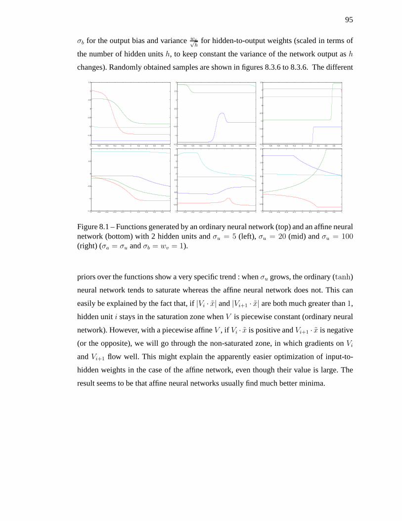
95

σb for the output bias and variancewv√h

for hidden-to-output weights (scaled in terms of

the number of hidden unitsh, to keep constant the variance of the network output ash

changes). Randomly obtained samples are shown in figures 8.3.6 to 8.3.6. The different

−1 −0.8 −0.6 −0.4 −0.2 0 0.2 0.4 0.6 0.8 1−2

−1.5

−1

−0.5

0

0.5

1

1.5

−1 −0.8 −0.6 −0.4 −0.2 0 0.2 0.4 0.6 0.8 1−1.5

−1

−0.5

0

0.5

1

1.5

2

−1 −0.8 −0.6 −0.4 −0.2 0 0.2 0.4 0.6 0.8 1−2.5

−2

−1.5

−1

−0.5

0

0.5

1

1.5

−1 −0.8 −0.6 −0.4 −0.2 0 0.2 0.4 0.6 0.8 1−1.5

−1

−0.5

0

0.5

1

−1 −0.8 −0.6 −0.4 −0.2 0 0.2 0.4 0.6 0.8 1−1

−0.5

0

0.5

1

1.5

2

2.5

3

3.5

4

−1 −0.8 −0.6 −0.4 −0.2 0 0.2 0.4 0.6 0.8 1−2

−1.5

−1

−0.5

0

0.5

1

1.5

2

2.5

Figure 8.1 – Functions generated by an ordinary neural network (top) and an affine neuralnetwork (bottom) with 2 hidden units andσu = 5 (left), σu = 20 (mid) andσu = 100(right) (σa = σu andσb = wv = 1).

priors over the functions show a very specific trend : whenσu grows, the ordinary (tanh)

neural network tends to saturate whereas the affine neural network does not. This can

easily be explained by the fact that, if|Vi · x| and|Vi+1 · x| are both much greater than1,

hidden uniti stays in the saturation zone whenV is piecewise constant (ordinary neural

network). However, with a piecewise affineV , if Vi · x is positive andVi+1 · x is negative

(or the opposite), we will go through the non-saturated zone, in which gradients onVi

andVi+1 flow well. This might explain the apparently easier optimization of input-to-

hidden weights in the case of the affine network, even though their value is large. The

result seems to be that affine neural networks usually find much better minima.

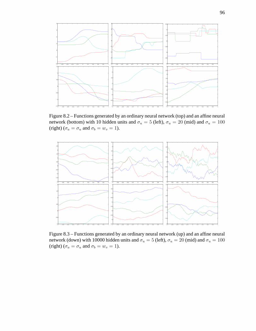
96

−1 −0.8 −0.6 −0.4 −0.2 0 0.2 0.4 0.6 0.8 1−2

−1

0

1

2

3

4

−1 −0.8 −0.6 −0.4 −0.2 0 0.2 0.4 0.6 0.8 1−4

−3

−2

−1

0

1

2

3

−1 −0.8 −0.6 −0.4 −0.2 0 0.2 0.4 0.6 0.8 1−4

−3.5

−3

−2.5

−2

−1.5

−1

−0.5

−1 −0.8 −0.6 −0.4 −0.2 0 0.2 0.4 0.6 0.8 1−1.5

−1

−0.5

0

0.5

1

1.5

−1 −0.8 −0.6 −0.4 −0.2 0 0.2 0.4 0.6 0.8 1−1

−0.5

0

0.5

1

1.5

2

2.5

−1 −0.8 −0.6 −0.4 −0.2 0 0.2 0.4 0.6 0.8 1−2

−1.5

−1

−0.5

0

0.5

1

1.5

2

2.5

3

Figure 8.2 – Functions generated by an ordinary neural network (top) and an affine neuralnetwork (bottom) with 10 hidden units andσu = 5 (left), σu = 20 (mid) andσu = 100(right) (σa = σu andσb = wv = 1).

−1 −0.8 −0.6 −0.4 −0.2 0 0.2 0.4 0.6 0.8 1−2

−1.5

−1

−0.5

0

0.5

1

1.5

2

2.5

3

−1 −0.8 −0.6 −0.4 −0.2 0 0.2 0.4 0.6 0.8 1−2

−1.5

−1

−0.5

0

0.5

1

1.5

2

2.5

−1 −0.8 −0.6 −0.4 −0.2 0 0.2 0.4 0.6 0.8 1−2

−1.5

−1

−0.5

0

0.5

1

1.5

2

−1 −0.8 −0.6 −0.4 −0.2 0 0.2 0.4 0.6 0.8 1−1

−0.5

0

0.5

1

1.5

2

−1 −0.8 −0.6 −0.4 −0.2 0 0.2 0.4 0.6 0.8 1−3.5

−3

−2.5

−2

−1.5

−1

−0.5

0

0.5

1

−1 −0.8 −0.6 −0.4 −0.2 0 0.2 0.4 0.6 0.8 1−2

−1.5

−1

−0.5

0

0.5

1

1.5

Figure 8.3 – Functions generated by an ordinary neural network (up) and an affine neuralnetwork (down) with 10000 hidden units andσu = 5 (left), σu = 20 (mid) andσu = 100(right) (σa = σu andσb = wv = 1).

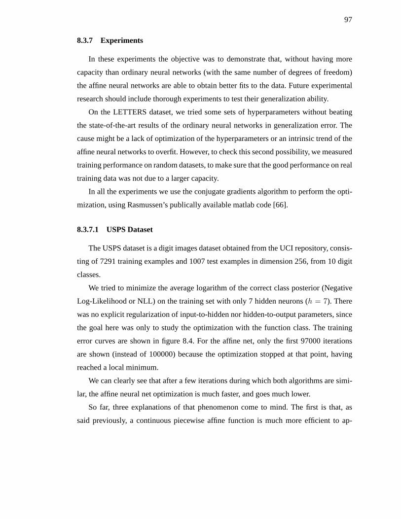
97

8.3.7 Experiments

In these experiments the objective was to demonstrate that,without having more

capacity than ordinary neural networks (with the same number of degrees of freedom)

the affine neural networks are able to obtain better fits to thedata. Future experimental

research should include thorough experiments to test theirgeneralization ability.

On the LETTERS dataset, we tried some sets of hyperparameters without beating

the state-of-the-art results of the ordinary neural networks in generalization error. The

cause might be a lack of optimization of the hyperparametersor an intrinsic trend of the

affine neural networks to overfit. However, to check this second possibility, we measured

training performance on random datasets, to make sure that the good performance on real

training data was not due to a larger capacity.

In all the experiments we use the conjugate gradients algorithm to perform the opti-

mization, using Rasmussen’s publically available matlab code [66].

8.3.7.1 USPS Dataset

The USPS dataset is a digit images dataset obtained from the UCI repository, consis-

ting of 7291 training examples and 1007 test examples in dimension 256, from 10 digit

classes.

We tried to minimize the average logarithm of the correct class posterior (Negative

Log-Likelihood or NLL) on the training set with only 7 hiddenneurons (h = 7). There

was no explicit regularization of input-to-hidden nor hidden-to-output parameters, since

the goal here was only to study the optimization with the function class. The training

error curves are shown in figure 8.4. For the affine net, only the first 97000 iterations

are shown (instead of 100000) because the optimization stopped at that point, having

reached a local minimum.

We can clearly see that after a few iterations during which both algorithms are simi-

lar, the affine neural net optimization is much faster, and goes much lower.

So far, three explanations of that phenomenon come to mind. The first is that, as

said previously, a continuous piecewise affine function is much more efficient to ap-

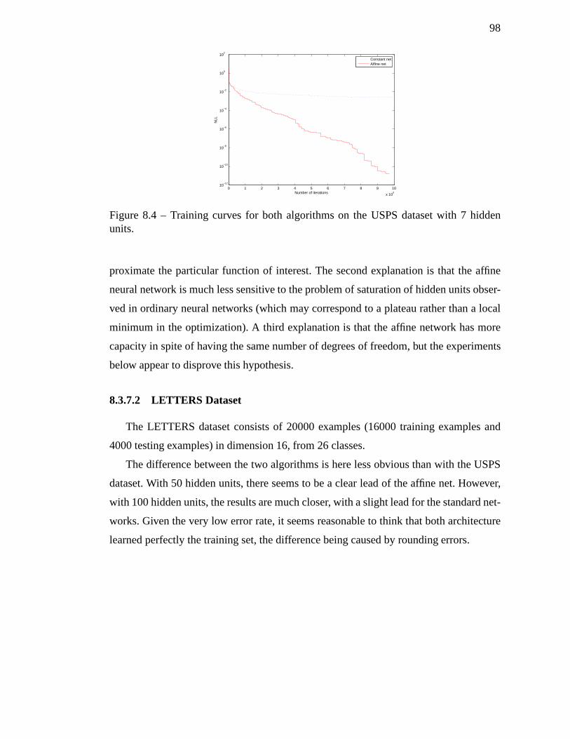
98

0 1 2 3 4 5 6 7 8 9 10

x 104

10−12

10−10

10−8

10−6

10−4

10−2

100

102

Number of iterations

NLL

Constant netAffine net

Figure 8.4 – Training curves for both algorithms on the USPS dataset with 7 hiddenunits.

proximate the particular function of interest. The second explanation is that the affine

neural network is much less sensitive to the problem of saturation of hidden units obser-

ved in ordinary neural networks (which may correspond to a plateau rather than a local

minimum in the optimization). A third explanation is that the affine network has more

capacity in spite of having the same number of degrees of freedom, but the experiments

below appear to disprove this hypothesis.

8.3.7.2 LETTERS Dataset

The LETTERS dataset consists of 20000 examples (16000 training examples and

4000 testing examples) in dimension 16, from 26 classes.

The difference between the two algorithms is here less obvious than with the USPS

dataset. With 50 hidden units, there seems to be a clear lead of the affine net. However,

with 100 hidden units, the results are much closer, with a slight lead for the standard net-

works. Given the very low error rate, it seems reasonable to think that both architecture

learned perfectly the training set, the difference being caused by rounding errors.

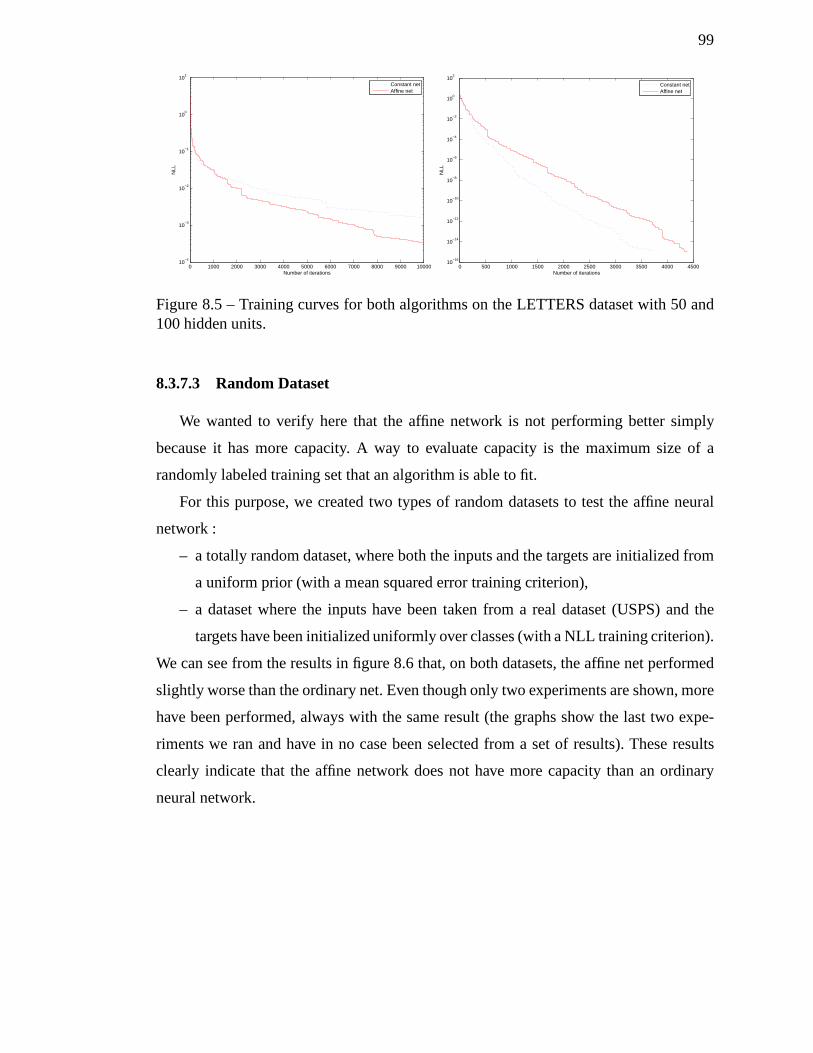
99

0 1000 2000 3000 4000 5000 6000 7000 8000 9000 1000010

−4

10−3

10−2

10−1

100

101

Number of iterations

NLL

Constant netAffine net

0 500 1000 1500 2000 2500 3000 3500 4000 450010

−16

10−14

10−12

10−10

10−8

10−6

10−4

10−2

100

102

Number of iterations

NLL

Constant netAffine net

Figure 8.5 – Training curves for both algorithms on the LETTERS dataset with 50 and100 hidden units.

8.3.7.3 Random Dataset

We wanted to verify here that the affine network is not performing better simply

because it has more capacity. A way to evaluate capacity is the maximum size of a

randomly labeled training set that an algorithm is able to fit.

For this purpose, we created two types of random datasets to test the affine neural

network :

– a totally random dataset, where both the inputs and the targets are initialized from

a uniform prior (with a mean squared error training criterion),

– a dataset where the inputs have been taken from a real dataset (USPS) and the

targets have been initialized uniformly over classes (witha NLL training criterion).

We can see from the results in figure 8.6 that, on both datasets, the affine net performed

slightly worse than the ordinary net. Even though only two experiments are shown, more

have been performed, always with the same result (the graphsshow the last two expe-

riments we ran and have in no case been selected from a set of results). These results

clearly indicate that the affine network does not have more capacity than an ordinary

neural network.

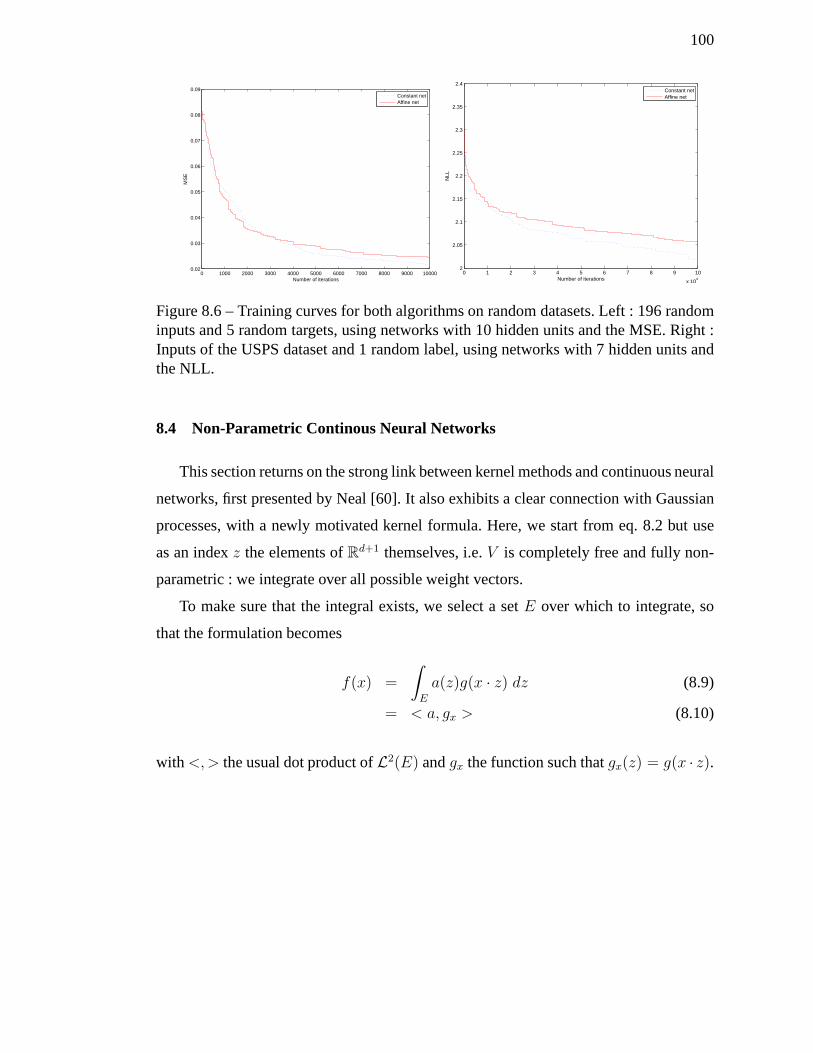
100

0 1000 2000 3000 4000 5000 6000 7000 8000 9000 100000.02

0.03

0.04

0.05

0.06

0.07

0.08

0.09

Number of iterations

MS

E

Constant netAffine net

0 1 2 3 4 5 6 7 8 9 10

x 104

2

2.05

2.1

2.15

2.2

2.25

2.3

2.35

2.4

Number of iterations

NLL

Constant netAffine net

Figure 8.6 – Training curves for both algorithms on random datasets. Left : 196 randominputs and 5 random targets, using networks with 10 hidden units and the MSE. Right :Inputs of the USPS dataset and 1 random label, using networkswith 7 hidden units andthe NLL.

8.4 Non-Parametric Continous Neural Networks

This section returns on the strong link between kernel methods and continuous neural

networks, first presented by Neal [60]. It also exhibits a clear connection with Gaussian

processes, with a newly motivated kernel formula. Here, we start from eq. 8.2 but use

as an indexz the elements ofRd+1 themselves, i.e.V is completely free and fully non-

parametric : we integrate over all possible weight vectors.

To make sure that the integral exists, we select a setE over which to integrate, so

that the formulation becomes

f(x) =

∫

E

a(z)g(x · z) dz (8.9)

= < a, gx > (8.10)

with <, > the usual dot product ofL2(E) andgx the function such thatgx(z) = g(x · z).

101

8.4.1 L1-norm Output Weights Regularization

Although the optimization problem becomes convex when theL1-norm ofa is pena-

lized, it involves an infinite number of variables. However,we are guaranteed to obtain a

finite number of hidden units with non-zero output weight, and both exact and approxi-

mate algorithms have been proposed for this case in [16]. Since this case has already

been well treated in that paper, we focus here on theL2 regularization case.

8.4.2 L2-norm Output Weights Regularization

In some cases, we know that the optimal functiona can be written as a linear combi-

nation of thegxiwith thexi’s the training examples. For example, when the cost function

is of the formc ((x1, y1, f(x1)), ..., (xm, ym, f(xm))) + Ω(‖f‖H) with ‖f‖H is the norm

induced by the kernelk defined byk(xi, xj) =< gxi, gxj

>, we can apply the representer

theorem [47].

It has been known for a decade that, with Gaussian priors overthe parameters, a

neural network with a number of hidden units growing to infinity converges to a Gaussian

process (chapter 2 of [60]). However, Neal did not compute explicitly the covariance

matrices associated to specific neural network architectures. Such covariance functions

have already been analytically computed [83], for the casesof sigmoid and Gaussian

transfer functions. However, this has been done using a Gaussian prior on the input-

to-hidden weights. The formulation presented here corresponds to a uniform prior (i.e.

with no arbitrary preference for particular values of the parameters) when the transfer

function issign. Thesign function has been used in [60] with a Gaussian prior on the

input-to-hidden weights, but the explicit covariance function could not be computed.

Instead, approximating locally the gaussian prior with a uniform prior, Neal ended up

with a covariance function of the formk(x, y) ≈ A−B||x− y||. We will see that, using

a uniform prior, this is exactly the form ofC one obtains.

102

8.4.3 Kernel wheng is the sign Function

8.4.3.1 Computation of the Kernel

For the sake of shorter notation, we will denote thesign function bys and warn the

reader not to get confused with thesigmoid function.

We wish to compute

k(x, y) =< gx, gy >= Ev,b [s(v · x + b)s(v · y + b)] .

Since we wish to define a uniform prior overv andb, we cannot let them span the whole

space (Rn in the case ofv andR in the case ofb). However, the value of the function

sign does not depend on the norm of its argument, so we can restrictourselves to the case

where‖v‖ = 1. Furthermore, for values ofb greater thanδ, whereδ is the maximum

norm among the samples, the value of the sign will be constantto 1 (and -1 for opposite

values ofb). Therefore, we only need to integrateb on the range[−δ, δ].

Defining a uniform prior on an interval depending on the training examples seems

contradictory. We will see later that, as long as the interval is big enough, its exact value

does not matter.

Let us first considerv fixed and compute the expectation overb. The product of two

sign functions is equal to 1 except when the argument of onesign is positive and the

other negative. In our case, this becomes :

v · x + b < 0

v · y + b > 0or

v · x + b > 0

v · y + b < 0

which is only true forb between−min(v · x, v · y) and−max(v · x, v · y), which is an

interval of size|v · x − v · y| = |v · (x − y)|.

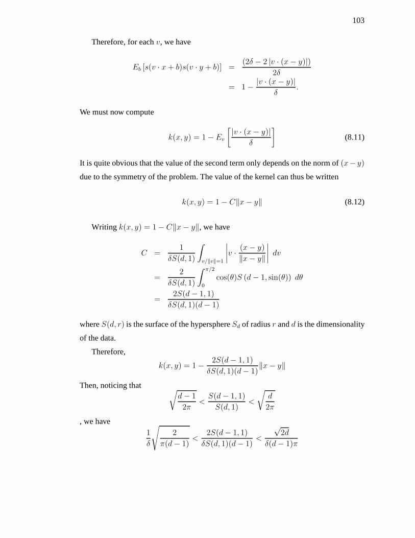
103

Therefore, for eachv, we have

Eb [s(v · x + b)s(v · y + b)] =(2δ − 2 |v · (x − y)|)

2δ

= 1 − |v · (x − y)|δ

.

We must now compute

k(x, y) = 1 − Ev

[ |v · (x − y)|δ

](8.11)

It is quite obvious that the value of the second term only depends on the norm of(x− y)

due to the symmetry of the problem. The value of the kernel canthus be written

k(x, y) = 1 − C‖x − y‖ (8.12)

Writing k(x, y) = 1 − C‖x − y‖, we have

C =1

δS(d, 1)

∫

v/‖v‖=1

∣∣∣∣v · (x − y)

‖x − y‖

∣∣∣∣ dv

=2

δS(d, 1)

∫ π/2

0

cos(θ)S (d − 1, sin(θ)) dθ

=2S(d − 1, 1)

δS(d, 1)(d− 1)

whereS(d, r) is the surface of the hypersphereSd of radiusr andd is the dimensionality

of the data.

Therefore,

k(x, y) = 1 − 2S(d − 1, 1)

δS(d, 1)(d− 1)‖x − y‖

Then, noticing that √d − 1

2π<

S(d − 1, 1)

S(d, 1)<

√d

2π

, we have1

δ

√2

π(d − 1)<

2S(d − 1, 1)

δS(d, 1)(d − 1)<

√2d

δ(d − 1)π

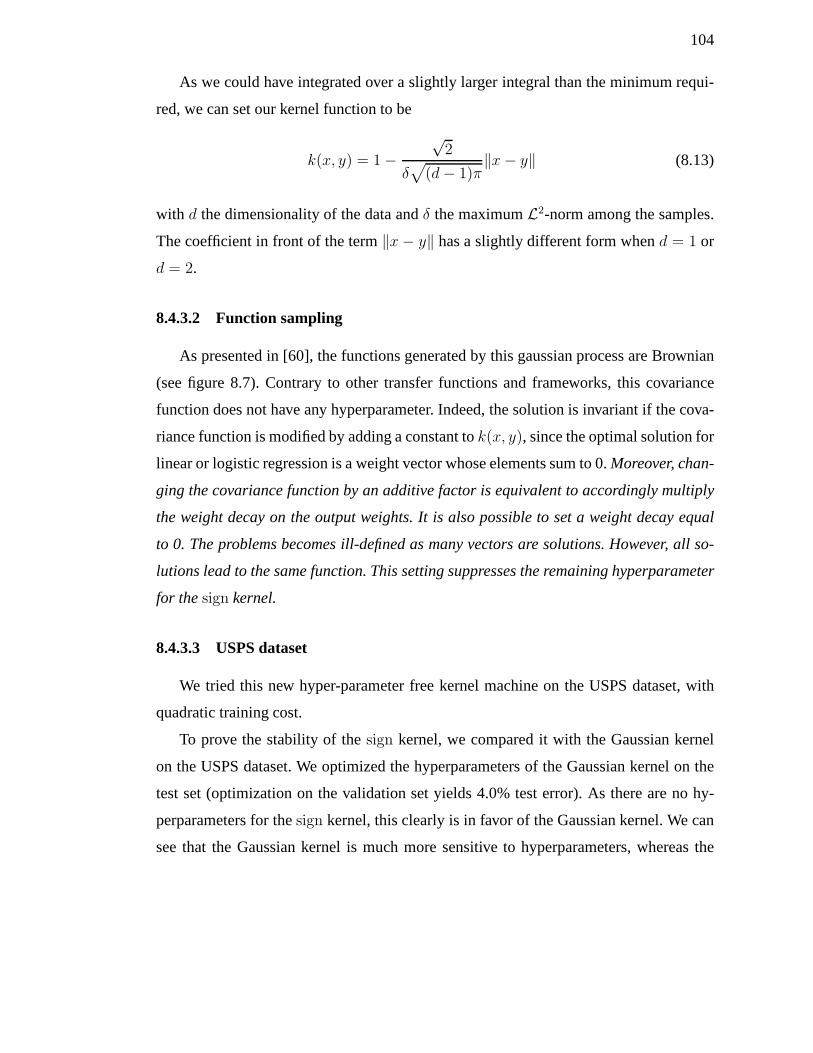
104

As we could have integrated over a slightly larger integral than the minimum requi-

red, we can set our kernel function to be

k(x, y) = 1 −√

2

δ√

(d − 1)π‖x − y‖ (8.13)

with d the dimensionality of the data andδ the maximumL2-norm among the samples.

The coefficient in front of the term‖x − y‖ has a slightly different form whend = 1 or

d = 2.

8.4.3.2 Function sampling

As presented in [60], the functions generated by this gaussian process are Brownian

(see figure 8.7). Contrary to other transfer functions and frameworks, this covariance

function does not have any hyperparameter. Indeed, the solution is invariant if the cova-

riance function is modified by adding a constant tok(x, y), since the optimal solution for

linear or logistic regression is a weight vector whose elements sum to 0.Moreover, chan-

ging the covariance function by an additive factor is equivalent to accordingly multiply

the weight decay on the output weights. It is also possible toset a weight decay equal

to 0. The problems becomes ill-defined as many vectors are solutions. However, all so-

lutions lead to the same function. This setting suppresses the remaining hyperparameter

for thesign kernel.

8.4.3.3 USPS dataset

We tried this new hyper-parameter free kernel machine on theUSPS dataset, with

quadratic training cost.

To prove the stability of thesign kernel, we compared it with the Gaussian kernel

on the USPS dataset. We optimized the hyperparameters of theGaussian kernel on the

test set (optimization on the validation set yields 4.0% test error). As there are no hy-

perparameters for thesign kernel, this clearly is in favor of the Gaussian kernel. We can

see that the Gaussian kernel is much more sensitive to hyperparameters, whereas the

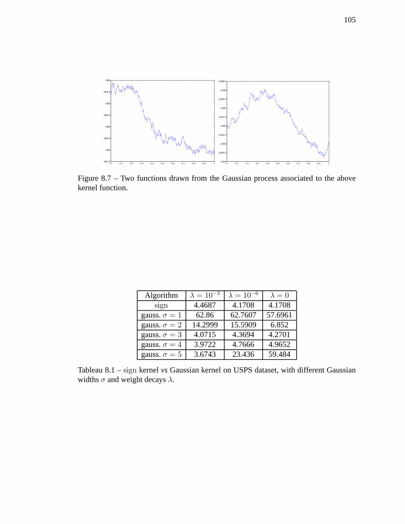
105

0 0.1 0.2 0.3 0.4 0.5 0.6 0.7 0.8 0.9 1−867.5

−867

−866.5

−866

−865.5

−865

−864.5

−864

0 0.1 0.2 0.3 0.4 0.5 0.6 0.7 0.8 0.9 1−2444

−2443.5

−2443

−2442.5

−2442

−2441.5

−2441

−2440.5

−2440

−2439.5

Figure 8.7 – Two functions drawn from the Gaussian process associated to the abovekernel function.

Algorithm λ = 10−3 λ = 10−6 λ = 0sign 4.4687 4.1708 4.1708

gauss.σ = 1 62.86 62.7607 57.6961gauss.σ = 2 14.2999 15.5909 6.852gauss.σ = 3 4.0715 4.3694 4.2701gauss.σ = 4 3.9722 4.7666 4.9652gauss.σ = 5 3.6743 23.436 59.484

Tableau 8.1 –sign kernelvsGaussian kernel on USPS dataset, with different Gaussianwidthsσ and weight decaysλ.

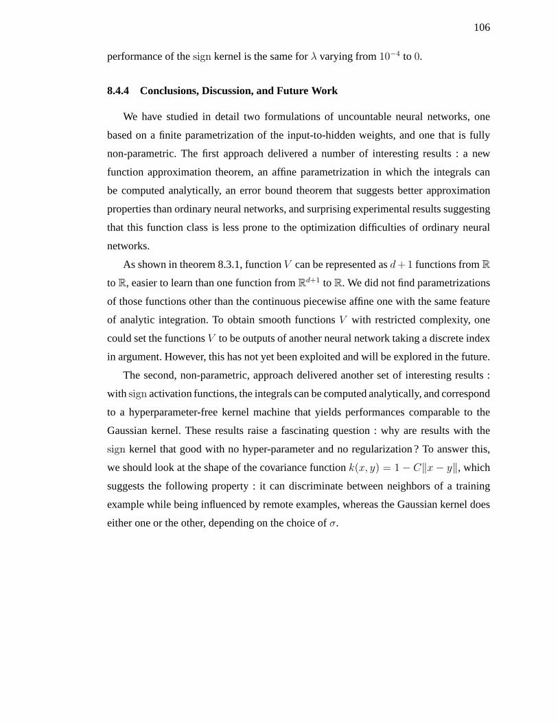
106

performance of thesign kernel is the same forλ varying from10−4 to 0.

8.4.4 Conclusions, Discussion, and Future Work

We have studied in detail two formulations of uncountable neural networks, one

based on a finite parametrization of the input-to-hidden weights, and one that is fully

non-parametric. The first approach delivered a number of interesting results : a new

function approximation theorem, an affine parametrizationin which the integrals can

be computed analytically, an error bound theorem that suggests better approximation

properties than ordinary neural networks, and surprising experimental results suggesting

that this function class is less prone to the optimization difficulties of ordinary neural

networks.

As shown in theorem 8.3.1, functionV can be represented asd+1 functions fromR

to R, easier to learn than one function fromRd+1 to R. We did not find parametrizations

of those functions other than the continuous piecewise affine one with the same feature

of analytic integration. To obtain smooth functionsV with restricted complexity, one

could set the functionsV to be outputs of another neural network taking a discrete index

in argument. However, this has not yet been exploited and will be explored in the future.

The second, non-parametric, approach delivered another set of interesting results :

with sign activation functions, the integrals can be computed analytically, and correspond

to a hyperparameter-free kernel machine that yields performances comparable to the

Gaussian kernel. These results raise a fascinating question : why are results with the

sign kernel that good with no hyper-parameter and no regularization ? To answer this,

we should look at the shape of the covariance functionk(x, y) = 1 − C‖x − y‖, which

suggests the following property : it can discriminate between neighbors of a training

example while being influenced by remote examples, whereas the Gaussian kernel does

either one or the other, depending on the choice ofσ.

CHAPITRE 9

PRÉSENTATION DU QUATRIÈME ARTICLE

9.1 Détails de l’article

Representational Power of Restricted Boltzmann Machines and Deep Belief Net-

works

N. Le Roux et Y. Bengio

À paraître dansNeural Computation, 20 :6, MIT Press, Cambridge, MAen 2008.

9.2 Contexte

Toutes les limitations des architectures peu profondes présentées dans les articles

précédents encouragèrent la recherche d’architectures réellement capables d’extraire des

concepts de haut niveau et insensibles au fléau de la dimensionnalité. De telles architec-

tures existaient déjà depuis 1989 [52] dans le contexte de lareconnaissance de caractères.

En 2006, Hinton et al. [39] proposèrent une méthode gloutonne pour entraîner des ré-

seaux profonds, et ce avec succès. Les Deep Belief Networks,ou DBN, obtinrent des ré-

sultats à l’état de l’art sur plusieurs ensembles de données, que ce soit en reconnaissance

de caractères ou en classification de documents. Contrairement aux réseaux à convo-

lution, les réseaux sigmoïdaux profonds ne sont pas limitésà une tâche particulière et

n’incluent pas de connaissance a priori sur le type de problème à résoudre.

9.2.1 Approches précédentes

9.2.1.1 Entraînement global

Les premières tentatives d’entraînement de réseaux profonds se firent en utilisant la

descente de gradient sur les paramètres de toutes les couches à la fois. Hormis pour cer-

taines architectures très précises [52], cette méthode tombait rapidement dans de mauvais

minima locaux. Deux raisons peuvent être invoquées pour cela.

108

La première est l’estompement du gradient. En effet, la présence d’une fonction de

transfert écrasante à chaque couche cachée diminue l’intensité du gradient au fur et à

mesure que l’on s’éloigne de la couche de sortie.

La deuxième est l’extrême complexité des relations entre les paramètres dès que l’on

s’éloigne de la couche de sortie. En effet, les poids de sortie agissent directement sur

la sortie de la fonction et n’ont que peu d’interactions. Dèslors que l’on parcourt les

couches cachées, les paramètres proches de la couche d’entrée interagissent au travers

des neurones cachées, rendant leur optimisation ardue.

Dans les deux cas, ce sont les paramètres les plus éloignés dela sortie (c’est-à-dire de

l’origine du signal de renforcement) qui sont les plus difficiles à optimiser. Cela motive

la création de méthodes d’entraînement n’optimisant que les paramètres proches de la

sortie.

9.2.1.2 Entraînement glouton

Des approches gloutonnes avaient été essayées auparavant pour entraîner des réseaux

profonds, mais sans succès. Elles consistaient en l’entraînement d’un réseau de neurones

à une couche cachée sur la tâche (supervisée) demandée [13].Les poids d’entrée étaient

alors fixés et les activations de la couche cachée obtenues enmettant les exemples d’en-

traînement en entrée devenaient les nouveaux exemples d’entraînement. Un nouveau

réseau de neurones à une couche cachée était alors entraîné sur ces exemples, et ainsi de

suite jusqu’à atteindre la profondeur voulue.

Malheureusement, cette technique souffre de la facilité del’apprentissage supervisé

sur l’ensemble d’apprentissage. En effet, si le nombre d’unités cachées est assez grand,

il est facile d’obtenir une erreur d’entraînement faible sur l’ensemble d’apprentissage,

et ce quels que soient les poids d’entrée. Autrement dit, un réseau de neurones à une

couche cachée n’a pas besoin d’extraire des caractéristiques pertinentes des données

pour parvenir à une faible erreur d’apprentissage. Cela a pour conséquence de jeter une

grande partie de l’information contenue dans l’ensemble d’entraînement lors du passage

à la première couche cachée. Ce problème est bien entendu amplifié à chaque ajout d’une

nouvelle couche.

109

Au contraire, les DBNs utilisent comme blocs de base des algorithmes non-supervisés,

les machines de Boltzmann restreintes (Restricted Boltzmann Machine, ou RBM). L’idée

fondatrice est qu’un algorithme non-supervisé va tenter deconserver toute l’information

contenue dans l’ensemble d’apprentissage et non seulementcelle nécessaire à la résolu-

tion du problème supervisé. L’avantage immédiat de cette méthode est la conservation

de l’information contenue dans les exemples d’apprentissage lors de l’ajout de couches.

Il est d’ailleurs intéressant de remarquer que d’autres méthodes proposant d’autres al-

gorithmes non-supervisés pour entraîner les couches ont obtenu des résultats compa-

rables [49].

Cette méthode possède toutefois un inconvénient majeur : avant la phase finale de

raffinement des paramètres, l’entraînement n’est aucunement guidé par la tâche supervi-

sée à réaliser. Cela devient problèmatique dès lors que seulle problème supervisé peut

être (approximativement) résolu en maintenant un modèle detaille raisonnable. Laro-

chelle et al. [49] tentèrent d’introduire un signal supervisé au cours de l’entraînement

des paramètres, améliorant quelque peu la performance finale.

9.3 Commentaires

L’article présenté ici s’intéresse exclusivement au modèle génératif et ne tient pas

compte d’un éventuel problème supervisé. Il démontre de manière constructive (contrai-

rement à [32], qui spécifient simplement que la machine de Boltzmann restreinte doit

agir comme une table de conversion, chaque unité cachée étant associée à un vecteur

d’entrée) l’universalité des machines de Boltzmann restreintes et propose une méthode

d’entraînement moins gloutonne que celle proposée par Hinton et al. [39]. Si cette

dernière permet d’obtenir de meilleurs résultats que la méthode initialement proposée

par Hinton et al. [39] sur des problèmes jouets, sa complexité la rend inexploitable pour

des problèmes réels.

En montrant que les machines de Boltzmann restreintes peuvent modéliser n’importe

quelle distribution et que leur puissance de représentation augmente strictement à l’ajout

d’une nouvelle unité cachée, cet article les relie plus fortement aux réseaux de neurones

110

habituels. En outre, la stratégie d’optimisation proposéemontre qu’il est théoriquement

possible d’effectuer un apprentissage efficace tout en étant moins glouton. Si l’algo-

rithme proposé dans cet article n’est pas exploitable en l’état, il n’en demeure pas moins

une source d’inspiration possible pour de futurs développements.

CHAPITRE 10

REPRESENTATIONAL POWER OF RESTRICTED BOLTZMANN

MACHINES AND DEEP BELIEF NETWORKS

10.1 Abstract

Deep Belief Networks (DBN) are generative neural network models with many layers

of hidden explanatory factors, recently introduced by Hinton et al., along with a greedy

layer-wise unsupervised learning algorithm. The buildingblock of a DBN is a probabi-

listic model called a Restricted Boltzmann Machine (RBM), used to represent one layer

of the model. Restricted Boltzmann Machines are interesting because inference is easy

in them, and because they have been successfully used as building blocks for training

deeper models. We first prove that adding hidden units yieldsstrictly improved model-

ling power, while a second theorem shows that RBMs are universal approximators of

discrete distributions. We then study the question of whether DBNs with more layers are

strictly more powerful in terms of representational power.This suggests a new and less

greedy criterion for training RBMs within DBNs.

10.2 Introduction

Learning algorithms that learn to represent functions withmany levels of compo-

sition are said to have adeep architecture. Bengio et Le Cun [15] discuss results in

computational theory of circuits that strongly suggest that deep architectures are much

more efficient in terms of representation (number of computational elements, number of

parameters) than their shallow counterparts. In spite of the fact that 2-level architectures

(e.g., a one-hidden layer neural network, a kernel machine,or a 2-level digital circuit)

are able to represent any function (see for example [44]), they may need a huge number

of elements and, consequently, of training examples. For example, the parity function on

d bits (which associates the value 1 with a vectorv if v has an odd number of bits equal

to 1 and0 otherwise) can be implemented by a digital circuit of depthlog(d) with O(d)

112

elements but requiresO(2d) elements to be represented by a 2-level digital circuit [2]

(e.g., in conjunctive or disjunctive normal form). We proved a similar result for Gaus-

sian kernel machines : they requireO(2d) non-zero coefficients (i.e., support vectors in

a Support Vector Machine) to represent such highly varying functions [10]. On the other

hand, training learning algorithms with a deep architecture (such as neural networks with

many hidden layers) appears to be a challenging optimization problem [13, 80].

Hinton et al. [39] introduced a greedy layer-wiseunsupervisedlearning algorithm for

Deep Belief Networks (DBN). The training strategy for such networks may hold great

promise as a principle to help address the problem of training deep networks. Upper

layers of a DBN are supposed to represent more “abstract” concepts that explain the

input data whereas lower layers extract “low-level features” from the data. In [13, 65],

this greedy layer-wise principle is found to be applicable to models other than DBNs.

DBNs and RBMs have already been applied successfully to a number of classification,

dimensionality reduction, information retrieval, and modelling tasks [13, 39, 42, 72, 82].

In this paper we show that adding hidden units yields strictly improved modelling

power, unless the RBM already perfectly models the data. Then, we prove that an RBM

can model any discrete distribution, a property similar to those of neural networks with

one hidden layer. Finally, we discuss the representationalpower of DBNs and find a

puzzling result about the best that could be achieved when going from 1-layer to 2-

layer DBNs. Note that the proofs of universal approximationby RBMs are constructive

but these constructions are not practical as they would leadto RBMs with potentially

as many hidden units as examples, and this would defy the purpose of using RBMs

as building blocks of a deep network that efficiently represents the input distribution.

Important theoretical questions therefore remain unanswered concerning the potential

for DBNs that stack multiple RBMs to represent a distribution efficiently.

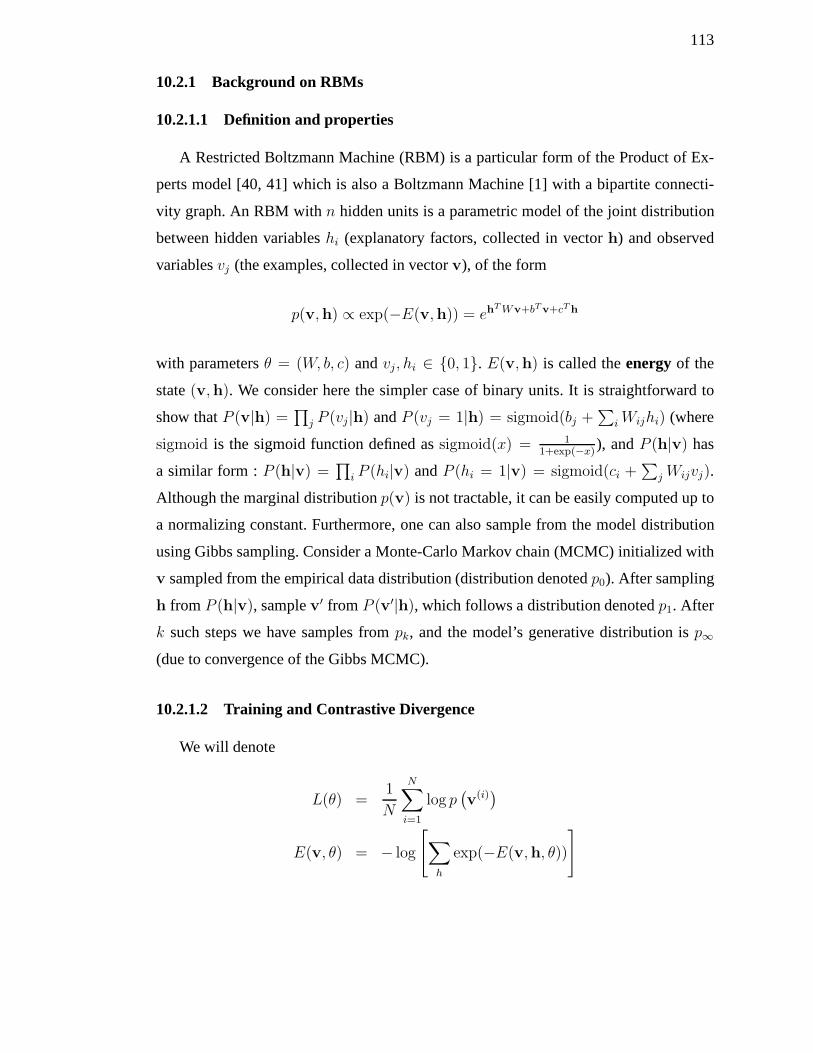
113

10.2.1 Background on RBMs

10.2.1.1 Definition and properties

A Restricted Boltzmann Machine (RBM) is a particular form ofthe Product of Ex-

perts model [40, 41] which is also a Boltzmann Machine [1] with a bipartite connecti-

vity graph. An RBM withn hidden units is a parametric model of the joint distribution

between hidden variableshi (explanatory factors, collected in vectorh) and observed

variablesvj (the examples, collected in vectorv), of the form

p(v,h) ∝ exp(−E(v,h)) = ehT Wv+bT

v+cTh

with parametersθ = (W, b, c) andvj, hi ∈ 0, 1. E(v,h) is called theenergy of the

state(v,h). We consider here the simpler case of binary units. It is straightforward to

show thatP (v|h) =∏

j P (vj|h) andP (vj = 1|h) = sigmoid(bj +∑

i Wijhi) (where

sigmoid is the sigmoid function defined assigmoid(x) = 11+exp(−x)

), andP (h|v) has

a similar form :P (h|v) =∏

i P (hi|v) andP (hi = 1|v) = sigmoid(ci +∑

j Wijvj).

Although the marginal distributionp(v) is not tractable, it can be easily computed up to

a normalizing constant. Furthermore, one can also sample from the model distribution

using Gibbs sampling. Consider a Monte-Carlo Markov chain (MCMC) initialized with

v sampled from the empirical data distribution (distribution denotedp0). After sampling

h from P (h|v), samplev′ from P (v′|h), which follows a distribution denotedp1. After

k such steps we have samples frompk, and the model’s generative distribution isp∞

(due to convergence of the Gibbs MCMC).

10.2.1.2 Training and Contrastive Divergence

We will denote

L(θ) =1

N

N∑

i=1

log p(v

(i))

E(v, θ) = − log

[∑

h

exp(−E(v,h, θ))

]

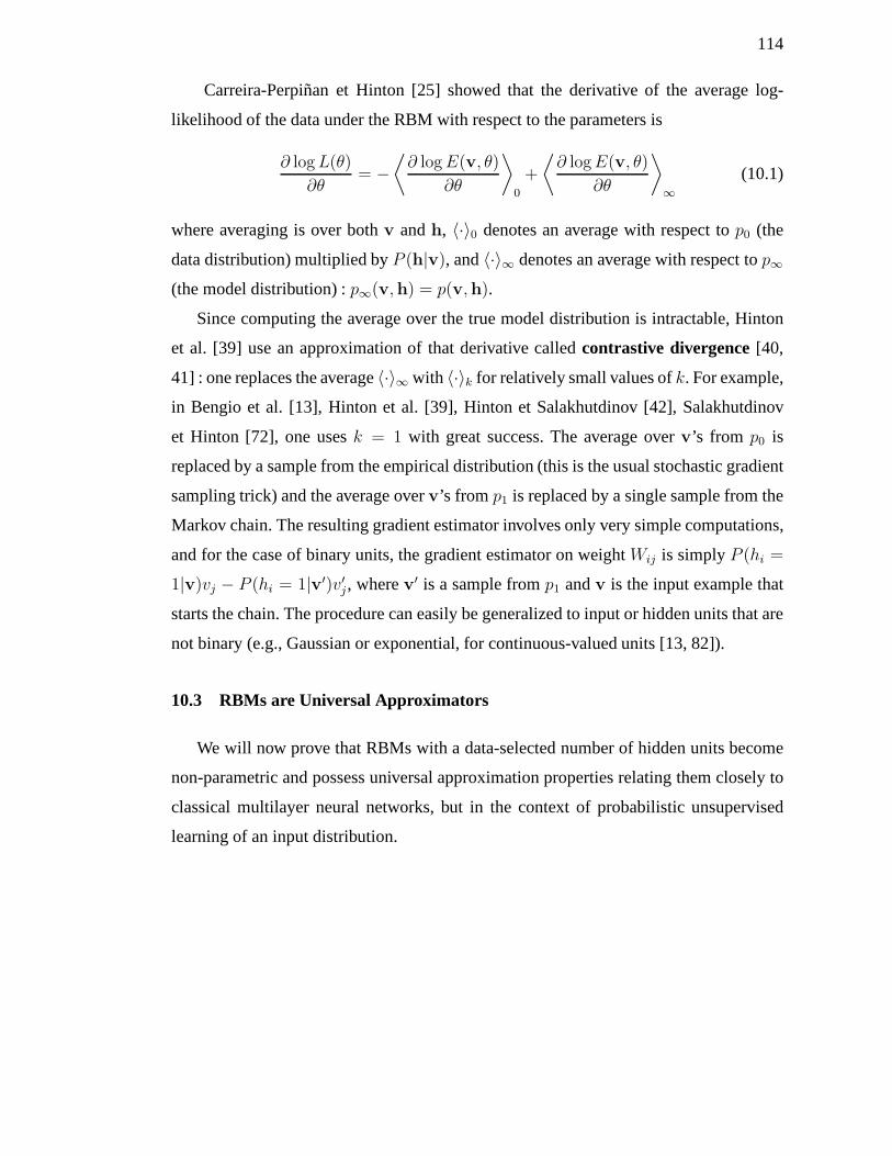
114

Carreira-Perpiñan et Hinton [25] showed that the derivative of the average log-

likelihood of the data under the RBM with respect to the parameters is

∂ log L(θ)

∂θ= −

⟨∂ log E(v, θ)

∂θ

⟩

0

+

⟨∂ log E(v, θ)

∂θ

⟩

∞(10.1)

where averaging is over bothv andh, 〈·〉0 denotes an average with respect top0 (the

data distribution) multiplied byP (h|v), and〈·〉∞ denotes an average with respect top∞

(the model distribution) :p∞(v,h) = p(v,h).

Since computing the average over the true model distribution is intractable, Hinton

et al. [39] use an approximation of that derivative calledcontrastive divergence[40,

41] : one replaces the average〈·〉∞ with 〈·〉k for relatively small values ofk. For example,

in Bengio et al. [13], Hinton et al. [39], Hinton et Salakhutdinov [42], Salakhutdinov

et Hinton [72], one usesk = 1 with great success. The average overv’s from p0 is

replaced by a sample from the empirical distribution (this is the usual stochastic gradient

sampling trick) and the average overv’s from p1 is replaced by a single sample from the

Markov chain. The resulting gradient estimator involves only very simple computations,

and for the case of binary units, the gradient estimator on weight Wij is simplyP (hi =

1|v)vj − P (hi = 1|v′)v′j , wherev′ is a sample fromp1 andv is the input example that

starts the chain. The procedure can easily be generalized toinput or hidden units that are

not binary (e.g., Gaussian or exponential, for continuous-valued units [13, 82]).

10.3 RBMs are Universal Approximators

We will now prove that RBMs with a data-selected number of hidden units become

non-parametric and possess universal approximation properties relating them closely to

classical multilayer neural networks, but in the context ofprobabilistic unsupervised

learning of an input distribution.

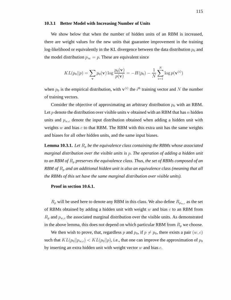
115

10.3.1 Better Model with Increasing Number of Units

We show below that when the number of hidden units of an RBM is increased,

there are weight values for the new units that guarantee improvement in the training

log-likelihood or equivalently in the KL divergence between the data distributionp0 and

the model distributionp∞ = p. These are equivalent since

KL(p0||p) =∑

v

p0(v) logp0(v)

p(v)= −H(p0) −

1

N

N∑

i=1

log p(v(i))

whenp0 is the empirical distribution, withv(i) theith training vector andN the number

of training vectors.

Consider the objective of approximating an arbitrary distribution p0 with an RBM.

Letp denote the distribution over visible unitsv obtained with an RBM that hasn hidden

units andpw,c denote the input distribution obtained when adding a hiddenunit with

weightsw and biasc to that RBM. The RBM with this extra unit has the same weights

and biases for all other hidden units, and the same input biases.

Lemma 10.3.1.LetRp be the equivalence class containing the RBMs whose associated

marginal distribution over the visible units isp. The operation of adding a hidden unit

to an RBM ofRp preserves the equivalence class. Thus, the set of RBMs composed of an

RBM ofRp and an additional hidden unit is also an equivalence class (meaning that all

the RBMs of this set have the same marginal distribution overvisible units).

Proof in section 10.6.1.

Rp will be used here to denote any RBM in this class. We also defineRpw,cas the set

of RBMs obtained by adding a hidden unit with weightw and biasc to an RBM from

Rp andpw,c the associated marginal distribution over the visible units. As demonstrated

in the above lemma, this does not depend on which particular RBM from Rp we choose.

We then wish to prove, that, regardlessp andp0, if p 6= p0, there exists a pair(w, c)

such thatKL(p0||pw,c) < KL(p0||p), i.e., that one can improve the approximation ofp0

by inserting an extra hidden unit with weight vectorw and biasc.

116

We will first state a trivial lemma needed for the rest of the proof. It says that inserting

a unit with biasc = −∞ does not change the input distribution associated with the RBM.

Lemma 10.3.2.Letp be the distribution over binary vectorsv in 0, 1d, obtained with

an RBMRp and letpw,c be the distribution obtained when adding a hidden unit with

weightsw and biasc to Rp. Then

∀p, ∀w ∈ Rd, p = pw,−∞

Démonstration.Denotingh =

h

hn+1

, W =

W

wT

andC =

C

c

wherewT

denotes the transpose ofw and introducingz(v,h) = exp(hT Wv + BTv + CT

h), we

can expressp(v,h) andpw,c(v, h) as follows :

p(v,h) ∝ z(v,h)

pw,c(v, h) ∝ exp(hT Wv + BT

v + CTh

)

∝ z(v,h) exp(hn+1w

Tv + chn+1

)

If c = −∞, pw,c(v, h) = 0 if hn+1 = 1. Thus, we can discard all terms wherehn+1 = 1,

keeping only those wherehn+1 = 0. Marginalizing over the hidden units, we have :

p(v) =

∑hz(v,h)∑

h(0),v0 z(v0,h(0))

pw,−∞(v) =

∑eh z(v,h) exp

(hn+1w

Tv + chn+1

)∑

gh(0),v0

z(v0,h(0)) exp(h

(0)n+1w

Tv + ch(0)n+1

)

=

∑hz(v,h) exp(0)∑

h(0),v0 z(v0,h(0)) exp(0)

= p(v)

We now state the main theorem.

117

Theorem 10.3.3.Letp0 be an arbitrary distribution over0, 1n and letRp be an RBM

with marginal distributionp over the visible units such thatKL(p0||p) > 0. Then there

exists an RBMRpw,ccomposed ofRp and an additional hidden unit with parameters

(w, c) whose marginal distributionpw,c over the visible units achievesKL(p0||pw,c) <

KL(p0||p).

Proof in section 10.6.2.

10.3.2 A Huge Model can Represent Any Distribution

The second set of results are for the limit case when the number of hidden units is

very large, so that we can represent any discrete distribution exactly.

Theorem 10.3.4.Any distribution over0, 1n can be approximated arbitrarily well (in

the sense of the KL divergence) with an RBM withk + 1 hidden units wherek is the

number of input vectors whose probability is not 0.

Proof sketch (Universal approximator property).We constructively build an RBM with

as many hidden units as the number of input vectors whose probability is strictly po-

sitive. Each hidden unit will be assigned to one input vector. Namely, whenvi is the

visible units vector, all hidden units have a probability0 of being on except the one

corresponding tovi which has a probabilitysigmoid(λi) of being on. The value ofλi

is directly tied withp(vi). On the other hand, when all hidden units are off but theith

one,p(vi|h) = 1. With probability1 − sigmoid(λi), all the hidden units are turned off,

which yields independent draws of the visible units. The proof consists in finding the

appropriate weights (and valuesλi) to yield that behaviour.

Proof in section 10.6.3.

118

10.4 Representational power of Deep Belief Networks

10.4.1 Background on Deep Belief Networks

A DBN with ℓ layers models the joint distribution between observed variablesvj and

ℓ hidden layersh(k), k = 1, . . . , ℓ made of binary unitsh(k)i (here all binary variables),

as follows :

p(v,h(1),h(2), . . . ,h(ℓ)) = P (v|h(1))P (h(1)|h(2)) . . . P (h(ℓ−2)|h(ℓ−1))p(h(ℓ−1),h(ℓ))

Denotingv = h(0), b(k) the bias vector of layerk andW (k) the weight matrix between

layerk and layerk + 1, we have :

P (h(k)|h(k+1)) =∏

i

P (h(k)i |h(k+1)) (factorial conditional distribution)

P (h(k)i = 1|h(k+1)) = sigmoid

(b(k)i +

∑

j

W(k)ij h

(k+1)j

)(10.2)

andp(h(ℓ−1),h(ℓ)) is an RBM.

The original motivation found in Hinton et al. [39] for having a deep network versus

a single hidden layer (i.e., a DBN versus an RBM) was that the representational power of

an RBM would be too limited and that more capacity could be achieved by having more

hidden layers. However, we have found here that an RBM with enough hidden units can

model any discrete distribution. Another motivation for deep architectures is discussed

in Bengio et Le Cun [15] and Bengio et al. [13] : deep architectures can represent func-

tions much more efficiently (in terms of number of required parameters) than shallow

ones. In particular, theoretical results on circuit complexity theory prove that shallow

digital circuits can be exponentially less efficient than deeper ones [2, 3, 37]. Hence the

original motivation [39] was probably right when one considers the restriction to reaso-

nably sized models.

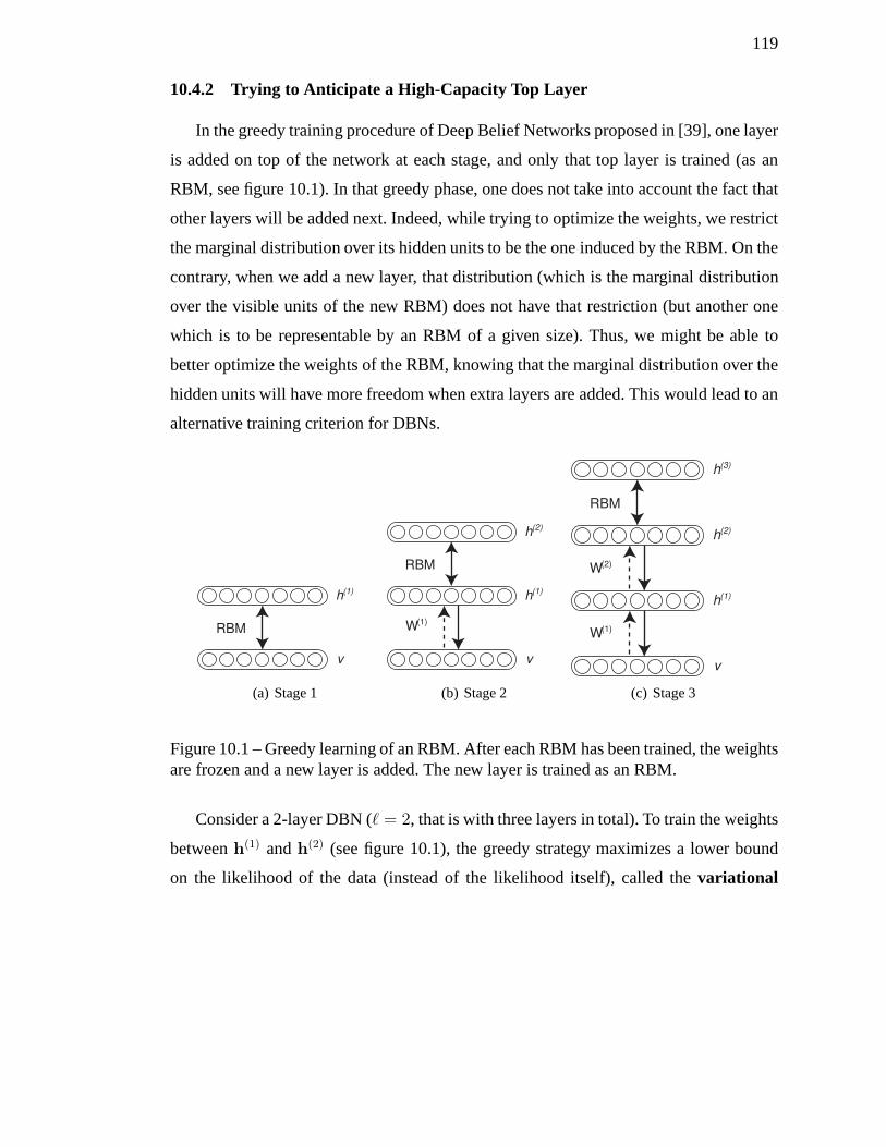
119

10.4.2 Trying to Anticipate a High-Capacity Top Layer

In the greedy training procedure of Deep Belief Networks proposed in [39], one layer

is added on top of the network at each stage, and only that top layer is trained (as an

RBM, see figure 10.1). In that greedy phase, one does not take into account the fact that

other layers will be added next. Indeed, while trying to optimize the weights, we restrict

the marginal distribution over its hidden units to be the oneinduced by the RBM. On the

contrary, when we add a new layer, that distribution (which is the marginal distribution

over the visible units of the new RBM) does not have that restriction (but another one

which is to be representable by an RBM of a given size). Thus, we might be able to

better optimize the weights of the RBM, knowing that the marginal distribution over the

hidden units will have more freedom when extra layers are added. This would lead to an

alternative training criterion for DBNs.

v

h(1)

RBM

(a) Stage 1

v

h(1)

h(2)

RBM

W(1)

(b) Stage 2

v

h(1)

h(2)

h(3)

RBM

W(1)

W(2)

(c) Stage 3

Figure 10.1 – Greedy learning of an RBM. After each RBM has been trained, the weightsare frozen and a new layer is added. The new layer is trained asan RBM.

Consider a 2-layer DBN (ℓ = 2, that is with three layers in total). To train the weights

betweenh(1) andh(2) (see figure 10.1), the greedy strategy maximizes a lower bound

on the likelihood of the data (instead of the likelihood itself), called thevariational

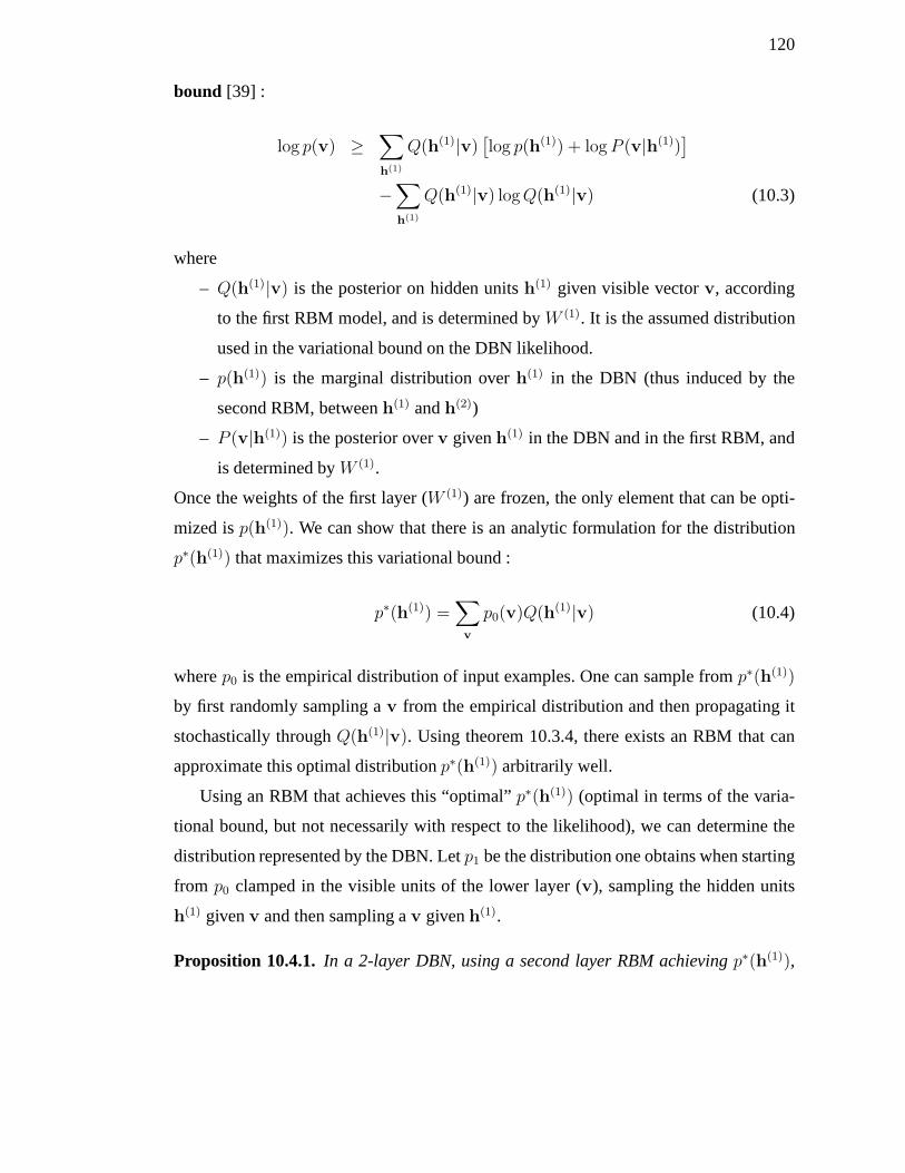
120

bound [39] :

log p(v) ≥∑

h(1)

Q(h(1)|v)[log p(h(1)) + log P (v|h(1))

]

−∑

h(1)

Q(h(1)|v) logQ(h(1)|v) (10.3)

where

– Q(h(1)|v) is the posterior on hidden unitsh(1) given visible vectorv, according

to the first RBM model, and is determined byW (1). It is the assumed distribution

used in the variational bound on the DBN likelihood.

– p(h(1)) is the marginal distribution overh(1) in the DBN (thus induced by the

second RBM, betweenh(1) andh(2))

– P (v|h(1)) is the posterior overv givenh(1) in the DBN and in the first RBM, and

is determined byW (1).

Once the weights of the first layer (W (1)) are frozen, the only element that can be opti-

mized isp(h(1)). We can show that there is an analytic formulation for the distribution

p∗(h(1)) that maximizes this variational bound :

p∗(h(1)) =∑

v

p0(v)Q(h(1)|v) (10.4)

wherep0 is the empirical distribution of input examples. One can sample fromp∗(h(1))

by first randomly sampling av from the empirical distribution and then propagating it

stochastically throughQ(h(1)|v). Using theorem 10.3.4, there exists an RBM that can

approximate this optimal distributionp∗(h(1)) arbitrarily well.

Using an RBM that achieves this “optimal”p∗(h(1)) (optimal in terms of the varia-

tional bound, but not necessarily with respect to the likelihood), we can determine the

distribution represented by the DBN. Letp1 be the distribution one obtains when starting

from p0 clamped in the visible units of the lower layer (v), sampling the hidden units

h(1) givenv and then sampling av givenh

(1).

Proposition 10.4.1. In a 2-layer DBN, using a second layer RBM achievingp∗(h(1)),

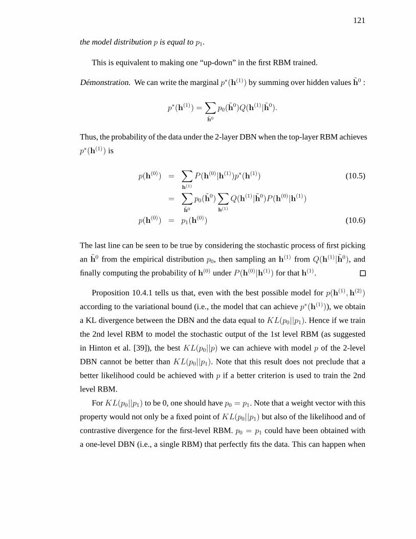
121

the model distributionp is equal top1.

This is equivalent to making one “up-down” in the first RBM trained.

Démonstration.We can write the marginalp∗(h(1)) by summing over hidden valuesh0 :

p∗(h(1)) =∑

h0

p0(h0)Q(h(1)|h0).

Thus, the probability of the data under the 2-layer DBN when the top-layer RBM achieves

p∗(h(1)) is

p(h(0)) =∑

h(1)

P (h(0)|h(1))p∗(h(1)) (10.5)

=∑

h0

p0(h0)∑

h(1)

Q(h(1)|h0)P (h(0)|h(1))

p(h(0)) = p1(h(0)) (10.6)

The last line can be seen to be true by considering the stochastic process of first picking

an h0 from the empirical distributionp0, then sampling anh(1) from Q(h(1)|h0), and

finally computing the probability ofh(0) underP (h(0)|h(1)) for thath(1).

Proposition 10.4.1 tells us that, even with the best possible model forp(h(1),h(2))

according to the variational bound (i.e., the model that canachievep∗(h(1))), we obtain

a KL divergence between the DBN and the data equal toKL(p0||p1). Hence if we train

the 2nd level RBM to model the stochastic output of the 1st level RBM (as suggested

in Hinton et al. [39]), the bestKL(p0||p) we can achieve with modelp of the 2-level

DBN cannot be better thanKL(p0||p1). Note that this result does not preclude that a

better likelihood could be achieved withp if a better criterion is used to train the 2nd

level RBM.

ForKL(p0||p1) to be 0, one should havep0 = p1. Note that a weight vector with this

property would not only be a fixed point ofKL(p0||p1) but also of the likelihood and of

contrastive divergence for the first-level RBM.p0 = p1 could have been obtained with

a one-level DBN (i.e., a single RBM) that perfectly fits the data. This can happen when

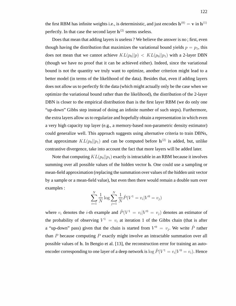
122

the first RBM has infinite weights i.e., is deterministic, andjust encodesh(0) = v in h(1)

perfectly. In that case the second layerh(2) seems useless.

Does that mean that adding layers is useless ? We believe the answer is no ; first, even

though having the distribution that maximizes the variational bound yieldsp = p1, this

does not mean that we cannot achieveKL(p0||p) < KL(p0||p1) with a 2-layer DBN

(though we have no proof that it can be achieved either). Indeed, since the variational

bound is not the quantity we truly want to optimize, another criterion might lead to a

better model (in terms of the likelihood of the data). Besides that, even if adding layers

does not allow us to perfectly fit the data (which might actually only be the case when we

optimize the variational bound rather than the likelihood), the distribution of the 2-layer

DBN is closer to the empirical distribution than is the first layer RBM (we do only one

“up-down” Gibbs step instead of doing an infinite number of such steps). Furthermore,

the extra layers allow us to regularize and hopefully obtaina representation in which even

a very high capacity top layer (e.g., a memory-based non-parametric density estimator)

could generalize well. This approach suggests using alternative criteria to train DBNs,

that approximateKL(p0||p1) and can be computed beforeh(2) is added, but, unlike

contrastive divergence, take into account the fact that more layers will be added later.

Note that computingKL(p0||p1) exactly is intractable in an RBM because it involves

summing over all possible values of the hidden vectorh. One could use a sampling or

mean-field approximation (replacing the summation over values of the hidden unit vector

by a sample or a mean-field value), but even then there would remain a double sum over

examples :N∑

i=1

1

Nlog

N∑

j=1

1

NP (V 1 = vi|V 0 = vj)

wherevi denotes thei-th example andP (V 1 = vi|V 0 = vj) denotes an estimator of

the probability of observingV 1 = vi at iteration 1 of the Gibbs chain (that is after

a “up-down” pass) given that the chain is started fromV 0 = vj. We write P rather

thanP because computingP exactly might involve an intractable summation over all

possible values ofh. In Bengio et al. [13], the reconstruction error for training an auto-

encoder corresponding to one layer of a deep network islog P (V 1 = vi|V 0 = vi). Hence

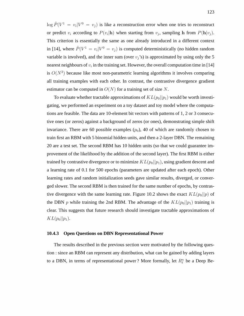
123

log P (V 1 = vi|V 0 = vj) is like a reconstruction error when one tries to reconstruct

or predictvi according toP (vi|h) when starting fromvj , samplingh from P (h|vj).

This criterion is essentially the same as one already introduced in a different context

in [14], whereP (V 1 = vi|V 0 = vj) is computed deterministically (no hidden random

variable is involved), and the inner sum (overvj ’s) is approximated by using only the 5

nearest neighbours ofvi in the training set. However, the overall computation time in [14]

is O(N2) because like most non-parametric learning algorithms it involves comparing

all training examples with each other. In contrast, the contrastive divergence gradient

estimator can be computed inO(N) for a training set of sizeN .

To evaluate whether tractable approximations ofKL(p0||p1) would be worth investi-

gating, we performed an experiment on a toy dataset and toy model where the computa-

tions are feasible. The data are 10-element bit vectors withpatterns of 1, 2 or 3 consecu-

tive ones (or zeros) against a background of zeros (or ones),demonstrating simple shift

invariance. There are 60 possible examples (p0), 40 of which are randomly chosen to

train first an RBM with 5 binomial hidden units, and then a 2-layer DBN. The remaining

20 are a test set. The second RBM has 10 hidden units (so that wecould guarantee im-

provement of the likelihood by the addition of the second layer). The first RBM is either

trained by contrastive divergence or to minimizeKL(p0||p1), using gradient descent and

a learning rate of 0.1 for 500 epochs (parameters are updatedafter each epoch). Other

learning rates and random initialization seeds gave similar results, diverged, or conver-

ged slower. The second RBM is then trained for the same numberof epochs, by contras-

tive divergence with the same learning rate. Figure 10.2 shows the exactKL(p0||p) of

the DBN p while training the 2nd RBM. The advantage of theKL(p0||p1) training is

clear. This suggests that future research should investigate tractable approximations of

KL(p0||p1).

10.4.3 Open Questions on DBN Representational Power

The results described in the previous section were motivated by the following ques-

tion : since an RBM can represent any distribution, what can be gained by adding layers

to a DBN, in terms of representational power ? More formally,let Rnℓ be a Deep Be-

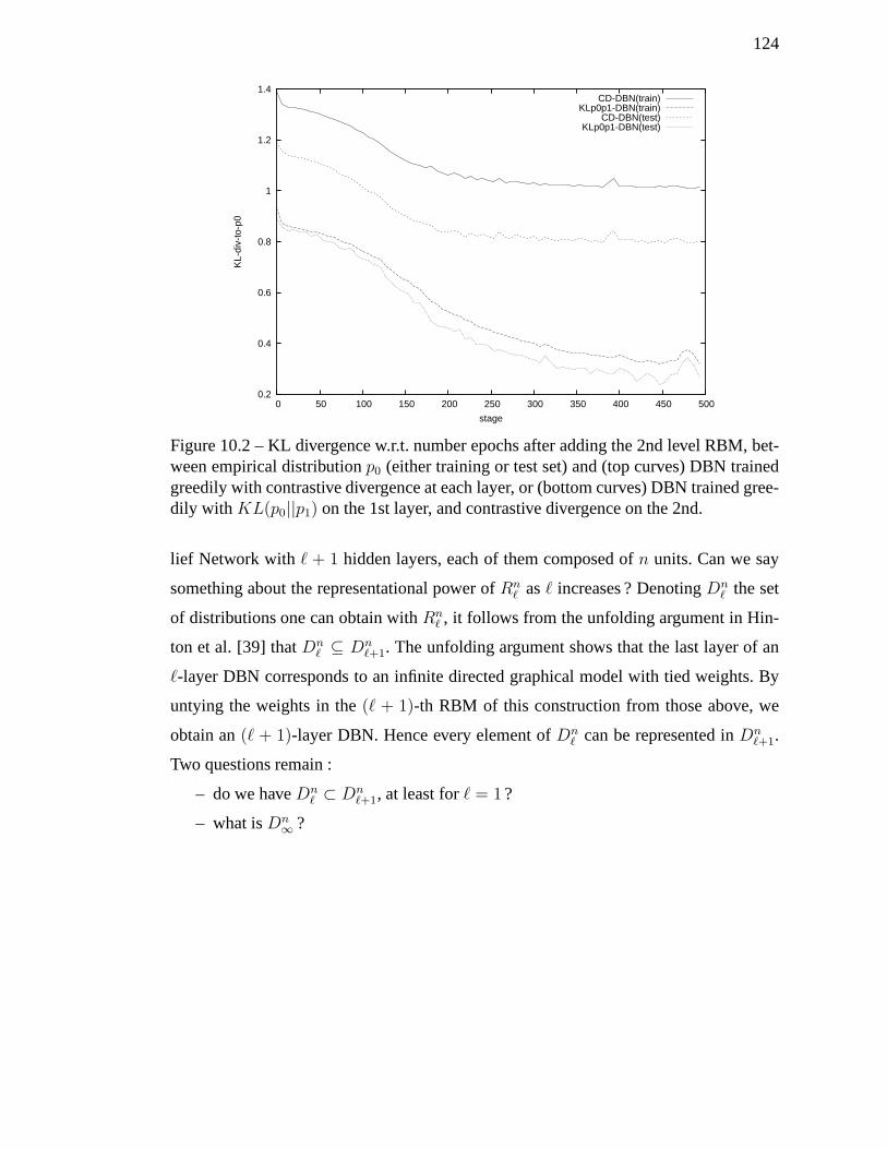
124

0.2

0.4

0.6

0.8

1

1.2

1.4

0 50 100 150 200 250 300 350 400 450 500

KL-

div-

to-p

0

stage

CD-DBN(train)KLp0p1-DBN(train)

CD-DBN(test)KLp0p1-DBN(test)

Figure 10.2 – KL divergence w.r.t. number epochs after adding the 2nd level RBM, bet-ween empirical distributionp0 (either training or test set) and (top curves) DBN trainedgreedily with contrastive divergence at each layer, or (bottom curves) DBN trained gree-dily with KL(p0||p1) on the 1st layer, and contrastive divergence on the 2nd.

lief Network with ℓ + 1 hidden layers, each of them composed ofn units. Can we say

something about the representational power ofRnℓ asℓ increases ? DenotingDn

ℓ the set

of distributions one can obtain withRnℓ , it follows from the unfolding argument in Hin-

ton et al. [39] thatDnℓ ⊆ Dn

ℓ+1. The unfolding argument shows that the last layer of an

ℓ-layer DBN corresponds to an infinite directed graphical model with tied weights. By

untying the weights in the(ℓ + 1)-th RBM of this construction from those above, we

obtain an(ℓ + 1)-layer DBN. Hence every element ofDnℓ can be represented inDn

ℓ+1.

Two questions remain :

– do we haveDnℓ ⊂ Dn

ℓ+1, at least forℓ = 1 ?

– what isDn∞ ?

125

10.5 Conclusions

We have shown that when the number of hidden units is allowed to vary, Restricted

Boltzmann Machines are very powerful and can approximate any distribution, eventually

representing them exactly when the number of hidden units isallowed to become very

large (possibly 2 to the number of inputs). This only says that parameter values exist for

doing so, but it does not prescribe how to obtain them efficiently. In addition, the above

result is only concerned with the case of discrete inputs. Itremains to be shown how to

extend that type of result to the case of continuous inputs.

Restricted Boltzmann Machines are interesting chiefly because they are the building

blocks of Deep Belief Networks, which can have many layers and can theoretically be

much more efficient at representing complicated distributions [15]. We have introduced

open questions about the expressive power of Deep Belief Networks. We have not ans-

wered these questions, but in trying to do so, we obtained an apparently puzzling result

concerning Deep Belief Networks : the best that can be achieved by adding a second

layer (with respect to some bound) is limited by the first layer’s ability to map the data

distribution to something close to itself (KL(p0||p1)), and this ability is good when the

first layer is large and models well the data. So why do we need the extra layers ? We

believe that the answer lies in the ability of a Deep Belief Network to generalize bet-

ter by having a more compact representation. This analysis also suggests to investigate

KL(p0||p1) (or an efficient approximation of it) as a less greedy alternative to contrastive

divergence for training each layer, because it would take into account that more layers

will be added.

Acknowledgements

The authors would like to thank the following funding organizations for support :

NSERC, MITACS, and the Canada Research Chairs. They are alsograteful for the help

and comments from Olivier Delalleau and Aaron Courville.

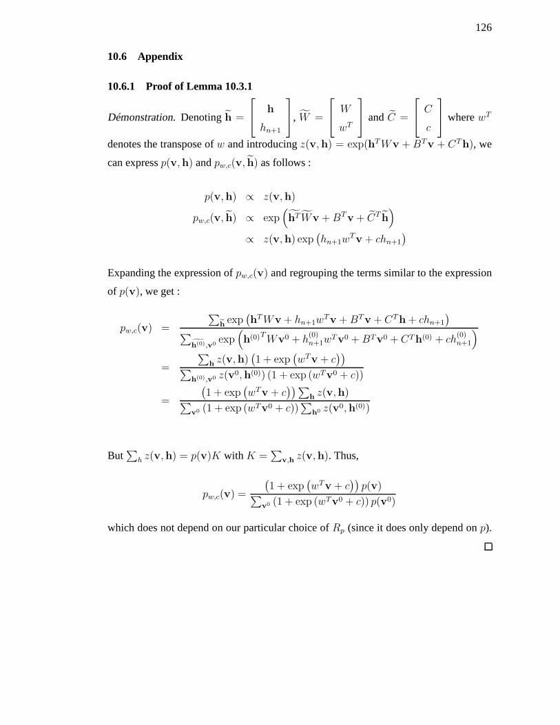
126

10.6 Appendix

10.6.1 Proof of Lemma 10.3.1

Démonstration.Denotingh =

h

hn+1

, W =

W

wT

andC =

C

c

wherewT

denotes the transpose ofw and introducingz(v,h) = exp(hT Wv + BTv + CT

h), we

can expressp(v,h) andpw,c(v, h) as follows :

p(v,h) ∝ z(v,h)

pw,c(v, h) ∝ exp(hT Wv + BT

v + CTh

)

∝ z(v,h) exp(hn+1w

Tv + chn+1

)

Expanding the expression ofpw,c(v) and regrouping the terms similar to the expression

of p(v), we get :

pw,c(v) =

∑eh exp

(h

T Wv + hn+1wTv + BT

v + CTh + chn+1

)∑

gh(0),v0

exp(h(0)T Wv0 + h

(0)n+1w

Tv0 + BTv0 + CTh(0) + ch(0)n+1

)

=

∑hz(v,h)

(1 + exp

(wT

v + c))

∑h(0),v0 z(v0,h(0)) (1 + exp (wTv0 + c))

=

(1 + exp

(wT

v + c))∑

hz(v,h)∑

v0 (1 + exp (wTv0 + c))∑

h0 z(v0,h(0))

But∑

h z(v,h) = p(v)K with K =∑

v,h z(v,h). Thus,

pw,c(v) =

(1 + exp

(wT

v + c))

p(v)∑v0 (1 + exp (wTv0 + c)) p(v0)

which does not depend on our particular choice ofRp (since it does only depend onp).

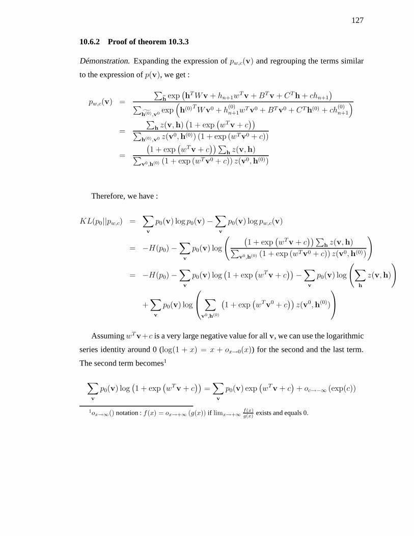
127

10.6.2 Proof of theorem 10.3.3

Démonstration.Expanding the expression ofpw,c(v) and regrouping the terms similar

to the expression ofp(v), we get :

pw,c(v) =

∑eh exp

(h

T Wv + hn+1wTv + BT

v + CTh + chn+1

)∑

gh(0),v0

exp(h(0)T Wv0 + h

(0)n+1w

Tv0 + BTv0 + CTh(0) + ch(0)n+1

)

=

∑hz(v,h)

(1 + exp

(wT

v + c))

∑h(0),v0 z(v0,h(0)) (1 + exp (wTv0 + c))

=

(1 + exp

(wT

v + c))∑

hz(v,h)∑

v0,h(0) (1 + exp (wTv0 + c)) z(v0,h(0))

Therefore, we have :

KL(p0||pw,c) =∑

v

p0(v) log p0(v) −∑

v

p0(v) log pw,c(v)

= −H(p0) −∑

v

p0(v) log

( (1 + exp

(wT

v + c))∑

hz(v,h)∑

v0,h(0) (1 + exp (wTv0 + c)) z(v0,h(0))

)

= −H(p0) −∑

v

p0(v) log(1 + exp

(wT

v + c))

−∑

v

p0(v) log

(∑

h

z(v,h)

)

+∑

v

p0(v) log

∑

v0,h(0)

(1 + exp

(wT

v0 + c

))z(v0,h(0))

AssumingwTv+c is a very large negative value for allv, we can use the logarithmic

series identity around 0 (log(1 + x) = x + ox→0(x)) for the second and the last term.

The second term becomes1

∑

v

p0(v) log(1 + exp

(wT

v + c))

=∑

v

p0(v) exp(wT

v + c)

+ oc→−∞ (exp(c))

1ox→∞() notation :f(x) = ox→+∞ (g(x)) if limx→+∞

f(x)g(x) exists and equals 0.

128

and the last term becomes

(∑

v

p0(v)

)log

∑

v0,h(0)

(1 + exp

(wT

v0 + c

))z(v0,h(0))

= log

∑

v0,h(0)

z(v0,h(0))

+ log

(1 +

∑v0,h(0) exp

(wT

v0 + c

)z(v0,h(0))

∑v0,h(0) z(v0,h(0))

)

= log

∑

v0,h(0)

z(v0,h(0))

+

∑v0,h(0) exp

(wT

v0 + c

)z(v0,h(0))∑

v0,h(0) z(v0,h(0))+ oc→−∞ (exp(c))

But

∑v0,h(0) exp

(wT

v0 + c

)z(v0,h(0))∑

v0,h(0) z(v0,h(0))=

∑

v

exp(wT

v + c) ∑

h(0) z(v,h(0))∑v0,h(0) z(v0,h(0))

=∑

v

exp(wT

v + c)p(v)

Putting all terms back together, we have

KL(p0||pw,c) = −H(p0) −∑

v

p0(v) exp(wT

v + c)

+∑

v

p(v) exp(wT

v + c)

+ oc→−∞ (exp(c)) −∑

v

p0(v) log

(∑

h

z(v,h)

)+ log

∑

v0,h(0)

z(v0,h(0))

= KL(p0||p) +∑

v

exp(wT

v + c)(p(v) − p0(v)) + oc→−∞ (exp(c))

Finally, we have

KL(p0||pw,c) − KL(p0||p) = exp(c)∑

v

exp(wT

v)(p(v) − p0(v)) + oc→−∞ (exp(c))(10.7)

129

The question now becomes : can we find aw such that∑

vexp

(wT

v)(p(v) − p0(v))

is negative?

As p0 6= p, there is av such thatp(v) < p0(v). Then there exists a positive scalara

such thatw = a

(v − 1

2e

)(with e = [1 . . . 1]T ) yields

∑vexp

(wT

v)(p(v) − p0(v)) <

0. Indeed, forv 6= v, we have

exp(wTv)

exp(wT v)= exp

(wT (v − v)

)

= exp

(a

(v − 1

2e

)T

(v − v)

)

= exp

(a∑

i

(vi −

1

2

)(vi − vi)

)

For i such thatvi − vi > 0, we havevi = 1 andvi = 0. Thus,vi − 12

= −12

and the

term inside the exponential is negative (sincea is positive). Fori such thatvi − vi < 0,

we havevi = 0 andvi = 1. Thus,vi − 12

= 12

and the term inside the exponential is also

negative. Furthermore, the terms come close to 0 asa goes to infinity. Since the sum can

be decomposed as

∑

v

exp(wT

v)(p(v) − p0(v)) = exp(wT

v)

(∑

v

exp(wT

v)

exp(wT v)(p(v) − p0(v))

)

= exp(wTv)

p(v) − p0(v) +

∑

v 6=bv

exp(wT

v)

exp(wT v)(p(v) − p0(v))

we have2

∑

v

exp(wT

v)(p(v) − p0(v)) ∼a→+∞ exp(wT

v)(p(v) − p0(v)) < 0.

Therefore, there is a valuea such that, ifa > a,∑

vexp

(wT

v)(p(v) − p0(v)) < 0.

This concludes the proof.

2∼x→∞ notation :f(x) ∼x→+∞ g(x) if limx→+∞

f(x)g(x) exists and equals 1.

130

10.6.3 Proof of theorem 10.3.4

Démonstration.In the former proof, we had

pw,c(v) =

(1 + exp

(wT

v + c))∑

hz(v,h)∑

v0,h(0) (1 + exp (wTv0 + c)) z(v0,h(0))

Let v be an arbitrary input vector andw be defined in the same way as before, i.e.

w = a

(v − 1

2

).

Now definec = −wTv + λ with λ ∈ R. We have :

lima→∞

1 + exp(wTv + c) = 1 for v 6= v

1 + exp(wTv + c) = 1 + exp(λ)

Thus, we can see that, forv 6= v :

lima→∞

p bw,bc(v) =

∑hz(v,h)∑

v0 6=v,h(0) z(v0,h(0)) +∑

h(0) (1 + exp (wT v + c)) z(v,h(0))

=

∑hz(v,h)∑

v0,h(0) z(v0,h(0)) +∑

h(0) exp (λ) z(v,h(0))

=

∑hz(v,h)∑

v0,h(0) z(v0,h(0))

1

1 + exp(λ)P

h(0) z(v,h(0))

Pv0,h(0) z(v0,h(0))

Rememberingp(v) =

∑hz(v,h)∑

v0,h(0) z(v0,h(0)), we have forv 6= v :

lima→∞

p bw,bc(v) =p(v)

1 + exp(λ)p(v)(10.8)

Similarly, we can see that

lima→∞

p bw,bc(v) =[1 + exp(λ)]p(v)

1 + exp(λ)p(v)(10.9)

Depending on the value ofλ, one can see that adding a hidden unit allows one to

increase the probability of an arbitraryv and to uniformly decrease the probability of

131

every otherv by a multiplicative factor. However, one can also see that, if p(v) = 0,

thenp bw,bc(v) = 0 for all λ.

We can therefore build the desired RBM as follows. Let us index thev’s over the

integers from 1 to2n and sort them such that

p0(vk+1) = . . . = p0(v2n) = 0 < p0(v1) ≤ p0(v2) ≤ . . . ≤ p0(vk)

Let us denotepi the distribution of an RBM withi hidden units. We start with an RBM

whose weights and biases are all equal to 0. The marginal distribution over the visible

units induced by that RBM is the uniform distribution. Thus,

p0(v1) = . . . = p0(v2n) = 2−n

We definew1 = a1(v1 − 12) andc1 = −wT

1 v1 + λ1.

As shown before, we now have :

lima1→+∞

p1(v1) =[1 + exp(λ1)]2

−n

1 + exp(λ1)2−n

lima1→+∞

p1(vi) =2−n

1 + exp(λ1)2−n∀i ≥ 2

As we can see, we can setp1(v1) to a value arbitrarily close to 1, with a uniform dis-

tribution overv2, . . . ,v2n . Then, we can chooseλ2 such thatp2(v2)

p2(v1)=

p(v2)

p(v1). This is

possible since we can arbitrarily increasep2(v2) while multiplying the other probabili-

ties by a constant factor and sincep(v2)

p(v1)≥ p1(v2)

p1(v1). We can continue the procedure until

obtainingpk(vk). The ratiopi(vj)

pi(vj−1)does not depend on the value ofi as long asi > j

(because at each such stepi, the two probabilities are multiplied by the same factor). We

will then have

pk(vk)

pk(vk−1)=

p(vk)

p(vk−1), . . . ,

pk(v2)

pk(v1)=

p(v2)

p(v1)

pk(vk+1) = . . . = pk(v2n)

132

From that, we can deduce thatpk(v1) = νkp(v1), . . . , pk(vk) = νkp(vk) with νk =

1 − (2n − k)pk(v2n).

We also havepk(v1)

pk(v2n)=

p1(v1)

p1(v2n)= 1 + exp(λ1).

Thus,pk(v1) = p(v1)[1 − (2n − k)pk(v2n)] = (1 + exp(λ1))pk(v2n).

Solving the above equations, we have

pk(vi) = p(v1)1+exp(λ1)+p(v1)(2n−k)

for i > k (10.10)

pk(vi) = p(vi)1+exp(λ1)

1+exp(λ1)+p(v1)(2n−k)for i ≤ k (10.11)

Using the logarithmic series identity around 0 (log(1 + x) = x + ox→0(x)) for

KL(p||pk) whenλ1 goes to infinity, we have

KL(p||pk) =∑

i

p(vi)(2n − k)p(vi)

1 + exp(λ1)+ o(exp(−λ1)) −→

λ1→∞0 (10.12)

This concludes the proof.

CHAPITRE 11

PRÉSENTATION DU CINQUIÈME ARTICLE

11.1 Détails de l’article

Topmoumoute Online Natural Gradient Algorithm

N. Le Roux, P.-A. Manzagol et Y. Bengio Publié dansAdvances in Neural Information

Processing Systems 20, MIT Press, Cambridge, MA en 2008.

11.2 Contexte

L’optimisation effectuée par un algorithme d’apprentissage nécessite la minimisation

d’un risqueL. Cette minimisation peut se faire de différentes façons, dépendamment des

structures deL et de notre algorithme.

Comme mentionné à la section 2.3, la descente de gradient estl’algorithme de choix

pour l’optimisation des réseaux de neurones ainsi que d’autres algorithmes impossibles

à optimiser analytiquement (ce qui est souvent le cas dès quel’on sort des algorithmes

triviaux).

Les algorithmes comme ceux mentionnés aux chapitres précédents possèdent un

grand nombre de paramètres et sont destinés à être entraînéssur un large ensemble

d’entraînement. On peut même imaginer un entraînement en continu nécessitant une

technique d’optimisation très rapide.

Le but de l’article présenté ici est de proposer un algorithme plus rapide que toutes

les méthodes de descente de gradient actuelles pour parvenir à entraîner des algorithmes

puissants sur des tâches difficiles.

11.3 Bilan

TONGA obtient des résultats extrêmement encourageants surplusieurs jeux de don-

nées importants. Il est toutefois judicieux de se demander pourquoi ses performances,

134

comparées à celles du gradient stochastique, diffèrent tant d’un jeu de données à l’autre.

L’une des raisons possibles est la supposition que les gradients sont tirés de manières

iid. Si cela est vrai dans le cas en ligne, ça devient une approximation dans le cas hors

ligne, approximation d’autant plus erronée que l’ensembled’apprentissage est petit. Ce

problème est relativement bénin puisque, dès lors que l’ensemble d’apprentissage est

petit, le besoin d’un algorithme d’optimisation rapide se fait moins ressentir.

Une autre possibilité est la sensibilité de cet algorithme aux hyperparamètres. En

effet, les valeurs deλ etγ sont primordiales pour l’efficacité de l’algorithme et un mau-

vais réglage peut entraîner des performances très décevantes. Il serait donc désirable

d’élaborer une méthode permettant le réglage automatique de ces paramètres.

CHAPITRE 12

TOPMOUMOUTE ONLINE NATURAL GRADIENT ALGORITHM

12.1 Abstract

Guided by the goal of obtaining an optimization algorithm that is both fast and yields

good generalization, we study the descent direction maximizing the decrease in generali-

zation error or the probability of not increasing generalization error. The surprising result

is that from both the Bayesian and frequentist perspectivesthis can yield the natural gra-

dient direction. Although that direction can be very expensive to compute we develop an

efficient, general, online approximation to the natural gradient descent which is suited to

large scale problems. We report experimental results showing much faster convergence

in computation time and in number of iterations with TONGA (Topmoumoute Online

Natural Gradient Algorithm) than with stochastic gradientdescent, even on very large

datasets.

Introduction

An efficient optimization algorithm is one that quickly findsa good minimum for a

given cost function. An efficient learning algorithm must dothe same, with the additional

constraint that the function is only known through a proxy. This work aims to improve

the ability to generalize through more efficient learning algorithms.

Consider the optimization of a cost on a training set with access to a validation set. As

the end objective is a good solution with respect to generalization, one often uses early

stopping : optimizing the training error while monitoring the validation error to fight

overfitting. This approach makes the underlying assumptionthat overfitting happens at

the later stages. A better perspective is that overfitting happens all through the learning,

but starts being detrimental only at the point it overtakes the “true” learning. In terms

of gradients, the gradient of the cost on the training set is never collinear with the true

gradient, and the dot product between the two actually eventually becomes negative.

136

Early stopping is designed to determine when that happens. One can thus wonder : can

one limit overfitting before that point ? Would this actuallypostpone that point ?

From this standpoint, we discover new justifications behindthe natural gradient [4].

Depending on certain assumptions, it corresponds either tothe direction minimizing the

probability of increasing generalization error, or to the direction in which the generaliza-

tion error is expected to decrease the fastest. Unfortunately, natural gradient algorithms

suffer from poor scaling properties, both with respect to computation time and memory,

when the number of parameters becomes large. To address thisissue, we propose a ge-

nerally applicable online approximation of natural gradient that scales linearly with the

number of parameters (and requires computation time comparable to stochastic gradient

descent). Experiments show that it can bring significant faster convergence and improved

generalization.

12.2 Natural gradient

Let L be a cost defined asL(θ) =

∫L(x, θ)p(x)dx whereL is a loss function

over some parametersθ and over the random variablex with distribution p(x). The

problem of minimizingL overθ is often encountered and can be quite difficult. There

exist various techniques to tackle it, their efficiency depending onL andp. In the case

of non-convex optimization, gradient descent is a successful technique. The approach

consists in progressively updatingθ using the gradientg = d eLdθ

.

Amari [4] showed that the parameter space is a Riemannian space of metricC (the

covariance of the gradients), and introduced the natural gradient as the direction of stee-

pest descent in this space. The natural gradient direction is therefore given byC−1g. The

Riemannian space is known to correspond to the space of functions represented by the

parameters (instead of the space of the parameters themselves).

The natural gradient somewhat resembles the Newton method.LeCun et al. [53] sho-

wed that, in the case of a mean squared cost function, the Hessian is equal to the sum

of the covariance matrix of the gradients and of an additional term that vanishes to0

as the training error goes down. Indeed, when the data are generated from the model,

137

the Hessian and the covariance matrix are equal. There are two important differences :

the covariance matrixC is positive-definite, which makes the technique more stable, but

contains no explicit second order information. The Hessianallows to account for varia-

tions in the parameters. The covariance matrix accounts forslight variations in the set

of training samples. It also means that, if the gradients highly disagree in one direction,

one should not go in that direction, even if the mean suggestsotherwise. In that sense, it

is a conservative gradient.

12.3 A new justification for natural gradient

Until now, we supposed we had access to the true distributionp. However, this is

usually not the case and, in general, the distributionp is only known through the samples

of the training set. These samples define a costL (resp. a gradientg) that, although close

to the true cost (resp. gradient), is not equal to it. We shallrefer toL as the training error

and toL as the generalization error. The danger is then to overfit theparametersθ to the

training set, yielding parameters that are not optimal withrespect to the generalization

error.

A simple way to fight overfitting consists in determining the point when the conti-

nuation of the optimization onL will be detrimental toL. This can be done by setting

aside some samples to form a validation set that will providean independent estimate of

L. Once the error starts increasing on the validation set, theoptimization should be stop-

ped. We propose a different perspective on overfitting. Instead of only monitoring the

validation error, we consider using as descent direction anestimate of the direction that

maximizes the probability of reducing the generalization error. The goal is to limit over-

fitting at every stage, with the hope that the optimal point with respect to the validation

should have lower generalization error.

Consider a descent directionv. We know that ifvT g is negative then the genera-

lization error drops (for a reasonably small step) when stepping in the direction ofv.

Likewise, if vT g is negative then the training error drops. Since the learning objective

is to minimize generalization error, we would likevT g as small as possible, or at least

138

always negative.

By definition, the gradient on the training set isg =1

n

n∑

i=1

gi wheregi =∂L(xi, θ)

∂θ

andn is the number of training samples. With a rough approximation, one can consider

the gis as draws from the true gradient distribution and assume allthe gradients are

independent and identically distributed. The central limit theorem then gives

g ∼ N

(g,

C

n

)(12.1)

whereC is the true covariance matrix of∂L(x,θ)∂θ

wrt p(x).

We will now show that, both in the Bayesian setting (with a Gaussian prior) and in

the frequentist setting (with some restrictions over the type of gradient considered), the

natural gradient is optimal in some sense.

12.3.1 Bayesian setting

In the Bayesian setting,g is a random variable. We would thus like to define a pos-

terior overg given the samplesgi in order to have a posterior distribution overvT g for

any given directionv. The prior overg will be a Gaussian centered in0 of varianceσ2I.

Thus, using eq. 12.1, the posterior overg given thegis (assuming the only information

over g given by thegis is throughg andC) is

g|g, C ∼ N

(

I +C

nσ2

)−1

g,

(I

σ2+ nC−1

)−1 (12.2)

DenotingCσ = I +eC

nσ2 , we therefore have

vT g|g, C ∼ N

(vT C−1

σ g,vT C−1

σ Cv

n

)(12.3)

Using this result, one can choose between several strategies, among which two are of

particular interest :

139

– choosing the directionv such that the expected value ofvT g is the lowest possible

(to maximize the immediate gain). In this setting, the direction v to choose is

v ∝ −C−1σ g. (12.4)

If σ < ∞, this is the regularized natural gradient. In the case ofσ = ∞, Cσ = I

and this is the batch gradient descent.

– choosing the directionv to minimize the probability ofvT g to be positive. This is

equivalent to finding

argminv

vT C−1σ g√

vT C−1σ Cv

(we droppedn for the sake of clarity, since it does not change the result).If we

square this quantity and take the derivative with respect tov, we find that the

numerator is equal to2C−1σ g(vT C−1

σ g)(vT C−1σ Cv)−2C−1

σ Cv(vT C−1σ g)2. The first

term is in the span ofC−1σ g and the second one is in the span ofC−1

σ Cv. Hence,

for the derivative to be zero, we must haveg ∝ Cv (sinceC andCσ are invertible),

i.e.

v ∝ −C−1g. (12.5)

This direction is the natural gradient and does not depend onthe value ofσ.

12.3.2 Frequentist setting

In the frequentist setting,g is a fixed unknown quantity. For the sake of simplicity,

we will only consider (as all second-order methods do) the directionsv of the form

v = MT g (i.e. we are only allowed to go in a direction which is a linearfunction ofg).

Sinceg ∼ N

(g,

eCn

), we have

vT g = gT Mg ∼ N

(gTMg,

gTMT CMg

n

)(12.6)

140

The matrixM∗ which minimizes the probability ofvT g to be positive satisfies

M∗ = argminM

gTMg

gTMT CMg(12.7)

The numerator of the derivative of this quantity isggTMT CMggT − 2CMggT MggT .

The first term is in the span ofg and the second one is in the span ofCMg. Thus, for

this derivative to be0 for all g, one must haveM ∝ C−1 and we obtain the same result

as in the Bayesian case : the natural gradient represents thedirection minimizing the

probability of increasing the generalization error.

12.4 Online natural gradient

The previous sections provided a number of justifications for using the natural gra-

dient. However, the technique has a prohibitive computational cost, rendering it imprac-

tical for large scale problems. Indeed, consideringp as the number of parameters andn

as the number of examples, a direct batch implementation of the natural gradient isO(p2)

in space andO(np2 + p3) in time, associated respectively with the gradients’ covariance

storage, computation and inversion. This section reviews existing low complexity im-

plementations of the natural gradient, before proposing TONGA, a new low complexity,

online and generally applicable implementation suited to large scale problems. In the

previous sections we assumed the true covariance matrixC to be known. In a practical

algorithm we of course use an empirical estimate, and here this estimate is furthermore

based on a low-rank approximation denotedC (actually a sequence of estimatesCt).

12.4.1 Low complexity natural gradient implementations

Yang et Amari [87] propose a method specific to the case of multilayer perceptrons.

By operating on blocks of the covariance matrix, this approach attains a lower com-

putational complexity1. However, the technique is quite involved, specific to multilayer

perceptrons and requires two assumptions : Gaussian distributed inputs and a number of

1Though the technique allows for a compact representation ofthe covariance matrix, the workingmemory requirement remains the same.

141

hidden units much inferior to that of input units. Amari et al. [5] offer a more general

approach based on the Sherman-Morrison formula used in Kalman filters : the technique

maintains an empirical estimate of the inversed covariancematrix that can be updated

in O(p2). Yet the memory requirement remainsO(p2). It is however not necessary to

compute the inverse of the gradients’ covariance, since oneonly needs its product with

the gradient. Yang et Amari [88] offer two approaches to exploit this. The first uses

conjugate gradient descent to solveCv = g. The second revisits [87] thereby achieving

a lower complexity. Schraudolph [78] also proposes an iterative technique based on the

minimization of a different cost. This technique is used in the minibatch setting, where

Cv can be computed cheaply through two matrix vector products.However, estimating

the gradient covariance only from a small number of examplesin one minibatch yields

unstable estimation.

12.4.2 TONGA

Existing techniques fail to provide an implementation of the natural gradient ade-

quate for the large scale setting. Their main failings are with respect to computational

complexity or stability. TONGA was designed to address these issues, which it does by

maintaining a low rank approximation of the covariance and by casting both problems

of finding the low rank approximation and of computing the natural gradient in a lower

dimensional space, thereby attaining a much lower complexity. What we exploit here

is that although a covariance matrix needs many gradients tobe estimated, we can take

advantage of an observed property that it generally varies smoothly as training proceeds

and moves in parameter space.

12.4.2.1 Computing the natural gradient direction betweentwo eigendecomposi-

tions

Even though our motivation for the use of natural gradient implied the covariance

matrix of the empirical gradients, we will use the second moment (i.e. the uncentered

covariance matrix) throughout the paper (and so did Amari inhis work). The main reason

142

is numerical stability. Indeed, in the batch setting, we have (assumingC is the centered

covariance matrix andg the mean)v = C−1g, thusCv = g. But then,(C + ggT )v =

g + ggTv = g(1 + gTv) and

(C + ggT )−1g =v

1 + gTv= v (12.8)

Even though the direction is the same, the scale changes and the norm of the direction is

bounded by 1‖g‖ cos(g,v)

.

Since TONGA operates using a low rank estimate of the gradients’ non-centered

covariance, we must be able to update cheaply. When presented with a new gradient, we

integrate its information using the following update formula2 :

Ct = γCt−1 + gtgTt (12.9)

whereC0 = 0 andCt−1 is the low rank approximation at time stept−1. Ct is now likely

of greater rank, and the problem resides in computing its lowrank approximationCt.

Writing Ct−1 = Xt−1XTt−1,

Ct = XtXTt with Xt = [

√γXt−1 gt]

With such covariance matrices, computing the (regularized) natural directionvt is equal

to

vt = (Ct + λI)−1gt = (XtXTt + λI)−1gt (12.10)

vt = (XtXTt + λI)−1Xtyt with yt = [0, . . . 0, 1]T . (12.11)

Using the Woodbury identity with positive definite matrices[64], we have

vt = Xt(XTt Xt + λI)−1yt (12.12)

2The second term is not weighted by1 − γ so that the influence ofgt in Ct is the same for allt,event = 0.To keep the magnitude of the matrix constant, one must use a normalization constant equal to1 + γ + . . . + γt.

143

If Xt is of sizep × r (with r < p, thus yielding a covariance matrix of rankr), the cost

of this computation isO(pr2 + r3). However, since the Gram matrixGt = XTt Xt can be

rewritten as

Gt =

γXT

t−1Xt−1√

γXTt−1gt

√γgT

t Xt−1 gTt gt

=

γGt−1

√γXT

t−1gt

√γgT

t Xt−1 gTt gt

, (12.13)

the cost of computingGt usingGt−1 reduces toO(pr + r3). This stresses the need to

keepr small.

12.4.2.2 Updating the low-rank estimate ofCt

To keep a low-rank estimate ofCt = XtXTt , we can compute its eigendecomposition

and keep only the firstk eigenvectors. This can be made at low cost using its relationto

that ofGt :

Gt = V DV T

Ct = (XtV D− 12 )D(XtV D− 1

2 )T (12.14)

The cost of such an eigendecomposition isO(kr2 + pkr) (for the computation of the

eigendecomposition of the Gram matrix and the computation of the eigenvectors, res-

pectively). Since the cost of computing the natural direction isO(pr + r3), it is compu-

tationally more efficient to let the rank ofXt grow for several steps (using formula 12.12

in between) and then compute the eigendecomposition using

Ct+b = Xt+bXTt+b with Xt+b =

[γUt, γ

b−12 gt+1, . . . γ

12 gt+b−1, γ

t+b2 gt+b]

]

with Ut the unnormalized eigenvectors computed during the previous eigendecomposi-

tion.

144

12.4.2.3 Computational complexity

The computational complexity of TONGA depends on the complexity of updating

the low rank approximation and on the complexity of computing the natural gradient.

The cost of updating the approximation is inO(k(k + b)2 + p(k + b)k) (as above, using

r = k + b). The cost of computing the natural gradientvt is in O(p(k + b) + (k + b)3)

(again, as above, usingr = k + b). Assumingk + b ≪√

(p) andk ≤ b, TONGA’s total

computational cost per each natural gradient computation is thenO(pb).

Furthermore, by operating on minibatch gradients of sizeb′, we end up with a cost

per example ofO( bpb′

). Choosingb = b′, yieldsO(p) per example, the same as stochastic

gradient descent. Empirical comparison of cpu time also shows comparable CPU time

per example, but faster convergence. In our experiments,p was in the tens of thousands,

k was less than 5 andb was less than50.

The result is an approximate natural gradient with low complexity, general applicabi-

lity and flexibility over the tradoff between computations and the quality of the estimate.

12.5 Block-diagonal online natural gradient for neural networks

One might wonder if there are better approximations of the covariance matrixC than

computing its firstk eigenvectors. One possibility is a block-diagonal approximation

from which to retain only the firstk eigenvectors of every block (the value ofk can

be different for each block). Indeed, [27] showed that the Hessian of a neural network

with one hidden layer trained with the cross-entropy cost converges to a block diagonal

matrix during optimization. These blocks are composed of the weights linking all the

hidden units to one output unit and all the input units to one hidden unit. Given the close

relationship between the Hessian and the covariance matrices, we can assume they have

a similar shape during the optimization.

Figure 12.1 shows the correlation between the standard stochastic gradients of the

parameters of a16 − 50 − 26 neural network. The first blocks represent the weights

going from the input units to each hidden unit (thus 50 blocksof size 17, bias included)

and the following represent the weights going from the hidden units to each output unit

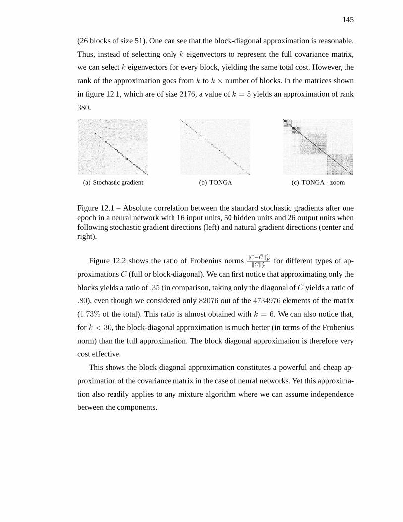
145

(26 blocks of size 51). One can see that the block-diagonal approximation is reasonable.

Thus, instead of selecting onlyk eigenvectors to represent the full covariance matrix,

we can selectk eigenvectors for every block, yielding the same total cost.However, the

rank of the approximation goes fromk to k × number of blocks. In the matrices shown

in figure 12.1, which are of size2176, a value ofk = 5 yields an approximation of rank

380.

(a) Stochastic gradient (b) TONGA (c) TONGA - zoom

Figure 12.1 – Absolute correlation between the standard stochastic gradients after oneepoch in a neural network with 16 input units, 50 hidden unitsand 26 output units whenfollowing stochastic gradient directions (left) and natural gradient directions (center andright).

Figure 12.2 shows the ratio of Frobenius norms‖C−C‖2F

‖C‖2F

for different types of ap-

proximationsC (full or block-diagonal). We can first notice that approximating only the

blocks yields a ratio of.35 (in comparison, taking only the diagonal ofC yields a ratio of

.80), even though we considered only82076 out of the4734976 elements of the matrix

(1.73% of the total). This ratio is almost obtained withk = 6. We can also notice that,

for k < 30, the block-diagonal approximation is much better (in termsof the Frobenius

norm) than the full approximation. The block diagonal approximation is therefore very

cost effective.

This shows the block diagonal approximation constitutes a powerful and cheap ap-

proximation of the covariance matrix in the case of neural networks. Yet this approxima-

tion also readily applies to any mixture algorithm where we can assume independence

between the components.

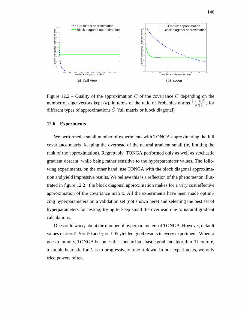
146

200 400 600 800 1000 1200 1400 1600 1800 20000

0.1

0.2

0.3

0.4

0.5

0.6

0.7

0.8

0.9

1

Number k of eigenvectors kept

Rat

io o

f the

squ

ared

Fro

beni

us n

orm

s

Full matrix approximationBlock diagonal approximation

(a) Full view

5 10 15 20 25 30 35 400.1

0.2

0.3

0.4

0.5

0.6

0.7

0.8

0.9

1

Number k of eigenvectors kept

Rat

io o

f the

squ

ared

Fro

beni

us n

orm

s

Full matrix approximationBlock diagonal approximation

(b) Zoom

Figure 12.2 – Quality of the approximationC of the covarianceC depending on the

number of eigenvectors kept (k), in terms of the ratio of Frobenius norms‖C−C‖2F

‖C‖2F

, for

different types of approximationsC (full matrix or block diagonal)

12.6 Experiments

We performed a small number of experiments with TONGA approximating the full

covariance matrix, keeping the overhead of the natural gradient small (ie, limiting the

rank of the approximation). Regrettably, TONGA performed only as well as stochastic

gradient descent, while being rather sensitive to the hyperparameter values. The follo-

wing experiments, on the other hand, use TONGA with the blockdiagonal approxima-

tion and yield impressive results. We believe this is a reflection of the phenomenon illus-

trated in figure 12.2 : the block diagonal approximation makes for a very cost effective

approximation of the covariance matrix. All the experiments have been made optimi-

zing hyperparameters on a validation set (not shown here) and selecting the best set of

hyperparameters for testing, trying to keep small the overhead due to natural gradient

calculations.

One could worry about the number of hyperparameters of TONGA. However, default

values ofk = 5, b = 50 andγ = .995 yielded good results in every experiment. Whenλ

goes to infinity, TONGA becomes the standard stochastic gradient algorithm. Therefore,

a simple heuristic forλ is to progressively tune it down. In our experiments, we only

tried powers of ten.

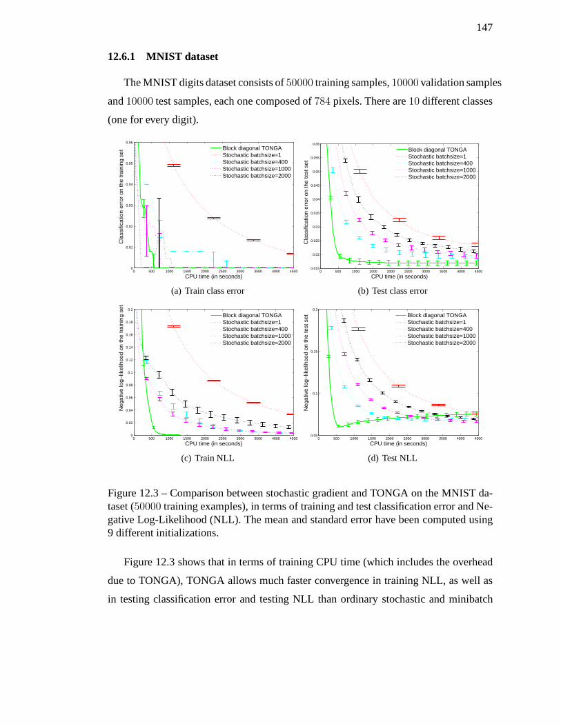
147

12.6.1 MNIST dataset

The MNIST digits dataset consists of50000 training samples,10000 validation samples

and10000 test samples, each one composed of784 pixels. There are10 different classes

(one for every digit).

0 500 1000 1500 2000 2500 3000 3500 4000 45000

0.01

0.02

0.03

0.04

0.05

0.06

CPU time (in seconds)

Cla

ssifi

catio

n er

ror

on th

e tr

aini

ng s

et

Block diagonal TONGAStochastic batchsize=1Stochastic batchsize=400Stochastic batchsize=1000Stochastic batchsize=2000

(a) Train class error

0 500 1000 1500 2000 2500 3000 3500 4000 45000.015

0.02

0.025

0.03

0.035

0.04

0.045

0.05

0.055

0.06

CPU time (in seconds)

Cla

ssifi

catio

n er

ror

on th

e te

st s

et

Block diagonal TONGAStochastic batchsize=1Stochastic batchsize=400Stochastic batchsize=1000Stochastic batchsize=2000

(b) Test class error

0 500 1000 1500 2000 2500 3000 3500 4000 45000

0.02

0.04

0.06

0.08

0.1

0.12

0.14

0.16

0.18

0.2

CPU time (in seconds)

Neg

ativ

e lo

g−lik

elih

ood

on th

e tr

aini

ng s

et

Block diagonal TONGAStochastic batchsize=1Stochastic batchsize=400Stochastic batchsize=1000Stochastic batchsize=2000

(c) Train NLL

0 500 1000 1500 2000 2500 3000 3500 4000 45000.05

0.1

0.15

0.2

CPU time (in seconds)

Neg

ativ

e lo

g−lik

elih

ood

on th

e te

st s

et

Block diagonal TONGAStochastic batchsize=1Stochastic batchsize=400Stochastic batchsize=1000Stochastic batchsize=2000

(d) Test NLL

Figure 12.3 – Comparison between stochastic gradient and TONGA on the MNIST da-taset (50000 training examples), in terms of training and test classification error and Ne-gative Log-Likelihood (NLL). The mean and standard error have been computed using9 different initializations.

Figure 12.3 shows that in terms of training CPU time (which includes the overhead

due to TONGA), TONGA allows much faster convergence in training NLL, as well as

in testing classification error and testing NLL than ordinary stochastic and minibatch

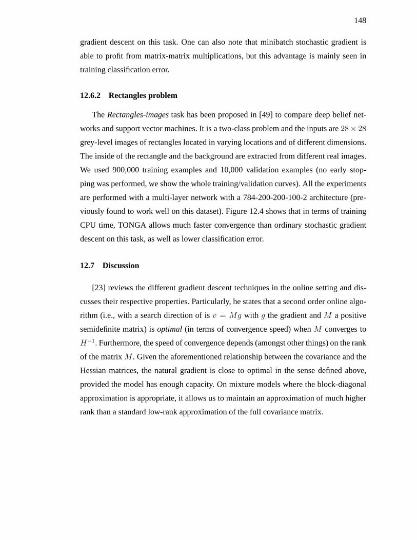
148

gradient descent on this task. One can also note that minibatch stochastic gradient is

able to profit from matrix-matrix multiplications, but thisadvantage is mainly seen in

training classification error.

12.6.2 Rectangles problem

The Rectangles-imagestask has been proposed in [49] to compare deep belief net-

works and support vector machines. It is a two-class problemand the inputs are28× 28

grey-level images of rectangles located in varying locations and of different dimensions.

The inside of the rectangle and the background are extractedfrom different real images.

We used 900,000 training examples and 10,000 validation examples (no early stop-

ping was performed, we show the whole training/validation curves). All the experiments

are performed with a multi-layer network with a 784-200-200-100-2 architecture (pre-

viously found to work well on this dataset). Figure 12.4 shows that in terms of training

CPU time, TONGA allows much faster convergence than ordinary stochastic gradient

descent on this task, as well as lower classification error.

12.7 Discussion

[23] reviews the different gradient descent techniques in the online setting and dis-

cusses their respective properties. Particularly, he states that a second order online algo-

rithm (i.e., with a search direction of isv = Mg with g the gradient andM a positive

semidefinite matrix) isoptimal (in terms of convergence speed) whenM converges to

H−1. Furthermore, the speed of convergence depends (amongst other things) on the rank

of the matrixM . Given the aforementioned relationship between the covariance and the

Hessian matrices, the natural gradient is close to optimal in the sense defined above,

provided the model has enough capacity. On mixture models where the block-diagonal

approximation is appropriate, it allows us to maintain an approximation of much higher

rank than a standard low-rank approximation of the full covariance matrix.

149

Conclusion and future work

We bring two main contributions in this paper. First, by looking for the descent di-

rection with either the greatest probability of not increasing generalization error or the

direction with the largest expected decrease in generalization error, we obtain new justifi-

cations for the natural gradient descent direction. Second, we present an online low-rank

approximation of natural gradient descent with computational complexity and CPU time

similar to stochastic gradient descent. In a number of experimental comparisons we find

this optimization technique to beat stochastic gradient interms of speed and generali-

zation (or in generalization for a given amount of training time). Even though default

values for the hyperparameters yield good results, it wouldbe interesting to have an

automatic procedure to select the best set of hyperparameters.

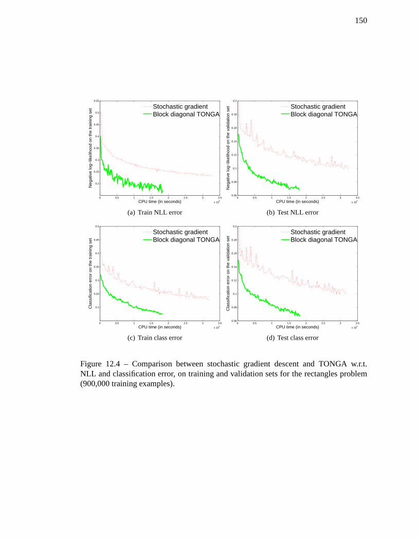
150

0 0.5 1 1.5 2 2.5 3 3.5

x 104

0.2

0.25

0.3

0.35

0.4

0.45

0.5

0.55

CPU time (in seconds)

Neg

ativ

e lo

g−lik

elih

ood

on th

e tr

aini

ng s

et

Stochastic gradientBlock diagonal TONGA

(a) Train NLL error

0 0.5 1 1.5 2 2.5 3 3.5

x 104

0.06

0.08

0.1

0.12

0.14

0.16

0.18

0.2

CPU time (in seconds)

Neg

ativ

e lo

g−lik

elih

ood

on th

e va

lidat

ion

set

Stochastic gradientBlock diagonal TONGA

(b) Test NLL error

0 0.5 1 1.5 2 2.5 3 3.5

x 104

0.2

0.25

0.3

0.35

0.4

0.45

0.5

CPU time (in seconds)

Cla

ssifi

catio

n er

ror

on th

e tr

aini

ng s

et

Stochastic gradientBlock diagonal TONGA

(c) Train class error

0 0.5 1 1.5 2 2.5 3 3.5

x 104

0.06

0.08

0.1

0.12

0.14

0.16

0.18

0.2

CPU time (in seconds)

Cla

ssifi

catio

n er

ror

on th

e va

lidat

ion

set

Stochastic gradientBlock diagonal TONGA

(d) Test class error

Figure 12.4 – Comparison between stochastic gradient descent and TONGA w.r.t.NLL and classification error, on training and validation sets for the rectangles problem(900,000 training examples).

CHAPITRE 13

CONCLUSION

Les articles de cette thèse s’inscrivent dans une démarche de compréhension des

limites des algorithmes majoritairement utilisés à l’heure actuelle et d’exploration de

nouvelles méthodes pour pouvoir traiter les problèmes importants à venir.

Après avoir mis en évidence et étudié les limites intrinsèques de la majorité des mé-

thodes à noyau (chapitre 4), nous avons essayé d’en transférer les propriétés attractives

aux réseaux de neurones à une couche cachée : la convexité de leur optimisation (cha-

pitre 6) et l’exploitabilité de leur universalité (chapitre 8). Malheureusement, ces avan-

cées n’ont pas permis de vaincre la déficience fondamentabledont sont affublées ces

deux familles d’algorithmes : l’impossibilité d’apprendre des concepts de haut niveau.

Nous nous sommes donc tournés vers les réseaux de neurones à plusieurs couches

cachées dont la profondeur nous a semblé adaptée à l’extraction de tels concepts. Nous

appuyant sur les travaux de Hinton et al. [39] sur les Deep Belief Networks, nous avons

étudié certaines des propriétés de ces réseaux et proposé une méthode d’entraînement de

substitution (chapitre 10).

Puisque notre but est de pouvoir traiter les problèmes importants à venir, nous nous

sommes également intéressés à une méthode permettant l’analyse rapide d’un très grand

nombre de données et qui est particulièrement adaptée aux réseaux de neurones possé-

dant un nombre quelconque de couches cachées (chapitre 12).

13.1 Synthèse des articles

13.1.1 The Curse of Highly Variable Functions for Local Kernel Machines

Cet article ne propose pas d’algorithme mais est une critique argumentée des mé-

thodes utilisant un noyau local. Deux critiques ont fréquemment été émises à l’encontre

de ces arguments :

– la première invoquait le« no free lunch theorem» [86] : aucun algorithme ne

152

surpasse strictement un autre si l’on prend l’espérance surtous les problèmes pos-

sibles. Cet argument insinue que nous n’avons qu’exhibé (etmême construit) des

problèmes pour lesquels les méthodes à noyau faillissent, ce qui ne constitue pas

une preuve de leurs faiblesses. Toutefois, nous ne sommes pas intéressés par la

construction d’algorithmes performants sur tous les problèmes possibles (ce qui

est impossible, d’après le théorème mentionné ci-dessus),mais sur tous les pro-

blèmes que nous sommes à même de rencontrer dans notre monde.Partant de ce

postulat, il est facile de voir que nous n’avons pas exhibé des problèmes choisis

au hasard, mais bien des problèmes qui, s’ils sont d’apparence complexe, n’en

demeurent pas moins très simples à résoudre pour un humain.

– la seconde arguait qu’il était impossible de généraliser loin des exemples d’ap-

prentissage, et ce quel que soit l’algorithme utilisé. Certains algorithmes, cher-

chant des structures dans les données, prouvèrent qu’il n’en était rien (voir par

exemple Non-Local Manifold Parzen Windows [14]).

Bien qu’apparemment illégitimes, ces critiques soulèventtoutefois un point d’im-

portance : les humains parviennent sans souci à généraliserà des situations totalement

inconnues, ce que les algorithmes actuels ont encore bien dumal à faire. Si certains

y parviennent mieux que d’autres, nous sommes encore loin desavoir transférer notre

connaissance d’une région de l’espace à une autre.

13.1.2 Convex Neural Networks

Cet article présente un algorithme utile à la fois pour la classification et la régression.

Si l’idée originale était de prouver qu’il était possible d’entraîner un réseau de neurones

de manière convexe, les implications furent toutes autres.Tout d’abord, le lien établi

entre les réseaux de neurones et le boosting est d’importance puisqu’il apporte un nou-

veau point de vue des réseaux de neurones. Ensuite, cet article montre également qu’un

réseau entraîné de manière gloutonne peut être optimal. Si cette gloutonnerie est hori-

zontale (c’est-à-dire que ce sont les unités cachées et non les couches qui sont ajoutées

de manière gloutonne), cela donne de l’espoir pour les Deep Belief Networks.

153

13.1.3 Continuous Neural Networks

Les réseaux continus étaient une tentative d’accorder aux réseaux de neurones l’al-

léchante propriété d’approximation universelle. Les limites de cette méthode théorique-

ment puissante ont permis de mettre en exergue deux des défis qui attendent la com-

munauté de l’apprentissage machine dans les années à venir :l’extraction de concepts

de haut niveau et l’optimisation efficace des paramètres. Nebénéficiant d’aucune de ces

deux propriétés, les réseaux continus ne purent tirer le meilleur avantage de leur capacité.

13.1.4 Representational Power of Restricted Boltzmann Machines and Deep Be-

lief Networks

Répondant aux manques des algorithmes mentionnés dans les trois articles précé-

dents, les Deep Belief Networks regorgent de promesses. C’est cette raison qui nous a

poussé à investiguer leur puissance et les moyens optimaux pour les entraîner. Cet article

permet également de mieux saisir les liens étroits reliant les machines de Boltzmann res-

treintes aux réseaux de neurones usuels et la validité de leur utilisation comme première

étape de l’entraînement.

13.1.5 Topmoumoute Online Natural Gradient Algorithm

Comme mentionné ci-dessus, l’autre grand défi est l’optimisation d’algorithmes com-

plexes en temps réel. En effet, de plus en plus, l’afflux de données est submergeant et il

apparaît appréciable d’être capable de traiter toutes ces informations. TONGA est l’un

des premiers réels algorithmes de second ordre stochastiques, qui plus est capable de

battre le gradient stochastique sur les problèmes sur lesquels il a été testé.

13.2 Conclusion

Le but de cette thèse fut de mettre en lumière les limites et lepotentiel des différents

algorithmes utilisés dans la communauté. Si les algorithmes profonds semblent propo-

ser des solutions aux problèmes rencontrés actuellement, ils ne sont pas pour autant la

154

panacée. Les algorithmes gloutons de Hinton et al. [39] et deBengio et al. [13] sont

pour l’instant sous-optimaux et ne s’accordent pas bien d’un flux incessant de nouvelles

données.

On assiste également à une évolution du type de régularisation utilisée. Alors qu’il

était coutume auparavant de limiter le nombre de neurones cachés (et donc le nombre de

paramètres libres), les réseaux de neurones actuels utilisent un très grand nombre de pa-

ramètres tout en imposant des contraintes supplémentaires, que ce soit en liant les poids

(comme dans [52] ou [62]) ou en essayant de résoudre un problème plus compliqué [39].

La qualité des résultats obtenus par ces dernières méthodeslaisse à penser que l’un des

grands défis futurs sera d’intégrer dans les algorithmes d’apprentissage des méthodes de

régularisation dont la notion de simplicité induite imitera au mieux celle utilisée par les

humains.

On peut aussi se demander l’importance du caractère non supervisé de l’entraînement

préalable des Deep Belief Networks. N’est-ce qu’une méthode de régularisation, comme

mentionné précédemment, ou bien un bon modèle génératif est-il nécessaire pour obte-

nir un bon modèle discriminant ? S’il fut longtemps accepté dans la communauté que,

pour obtenir un modèle discriminant, il était inutile et même préjudiciable d’entraîner un

modèle génératif, Ng et Jordan [61] montrèrent qu’il pouvait être intéressant d’essayer

de modéliser toute la distribution jointe dans certains contextes. De leur côté, Lasserre

et al. [50] analysèrent les suppositions implicites d’un entraînement discriminant. Les

humains possèdent-ils réellement un modèle génératif du monde qui les entoure ? Est-ce

nécessaire ?

Enfin, l’autre défi qui attend la communauté de l’apprentissage machine est celui de

la multimodalité. En tant qu’humains, nous percevons des données de différents types

(selon le sens utilisé) que nous combinons de manière efficace pour résoudre les pro-

blèmes auxquels nous devons faire face. En outre, nous sommes parfaitement capables de

transférer nos connaissances abstraites acquises dans un contexte donné à des contextes

totalement différents. Il n’existe pas à l’heure actuelle d’algorithmes capables d’un tel

transfert.

Les algorithmes d’apprentissage futurs auront la nécessité de pouvoir extraire des

155

concepts de haut niveau en utilisant un nombre toujours plusgrand d’exemples si on

veut espérer atteindre un jour l’intelligence artificielle.

Index

étiquette, 5

entrée étiquetée, 5

a priori, 20, 35

algorithme

non-paramétrique, 10

paramétrique, 10

apprentissage, 1

non supervisé, 7

semi-supervisé, 9

supervisé, 5

arctangente, 32

Bayes

Apprentissage bayésien, 21, 22

Théorème, 19

biais

d’entrée, 31

de sortie, 31

classification, 5, 9

coût

fonction, 12

constante de normalisation, 20

convexité, 66

coordonnées

réduites, 9

covariance

fonction, 29

matrice, 27

cumulative, 32

descente de gradient, 37

distribution, 7

distribution de Laplace, 24

entrée, 5

erreur

entraînement, 12

test, 12

espace de caractéristiques, 26

estimation de densité, 7

feature space, 26

fonction écrasante, 31

fonction de transfert, 31

fonction logistique, 32

fonction sigmoïdale, 32

gaussien

processus, processus

gaussien, 29

gradient

156

157

descente de, 37

hyperparamètre, 27

machine de Boltzmann, 29

machine de Boltzmann restreinte, 29

maximum a posteriori, 21

moyenne

fonction, 29

norme

L1, 17

L2, 18

noyau, 26

astuce, 29

espace de Hilbert à noyau reproduisant,

27

fonction, 26

gaussien, 26

méthodes, 26

polynomial, 27

inhomogène, 27

sigmoïdal, 27

théorème du représentant, 28

perceptron, 29, 30

poids

d’entrée, 31

de sortie, 31

postérieur, 20

réduction de dimensionnalité, 9

régression, 5, 9

régularisation

coefficient, 17

réseau de neurones, 26, 29

à convolution, 29

à propagation avant, 29

profond, 34

regroupement, 8

représentant

théorème, 28

surapprentissage, 12

tangente hyperbolique, 32

vraisemblance, 20

BIBLIOGRAPHIE

[1] D.H. Ackley, G.E. Hinton et T.J. Sejnowski. A learning algorithm for Boltzmann

machines.Cognitive Science, 9:147–169, 1985.

[2] M. Ajtai.∑1

1-formulae on finite structures.Annals of Pure and Applied Logic,

(24):1–48, 1983.

[3] E. Allender. Circuit complexity before the dawn of the new millennium. Dans

16th Annual Conference on Foundations of Software Technology and Theoretical

Computer Science, pages 1–18. Lecture Notes in Computer Science 1180, Springer

Verlag, 1996.

[4] S. Amari. Natural gradient works efficiently in learning. Neural Compu-

tation, 10(2):251–276, 1998. URLciteseer.ist.psu.edu/article/

amari98natural.html.

[5] S. Amari, H. Park et K. Fukumizu. Adaptive method of realizing natural gradient

learning for multilayer perceptrons.Neural Computation, 12(6):1399–1409, 2000.

URL citeseer.ist.psu.edu/amari98adaptive.html.

[6] C.T.H. Baker. The numerical treatment of integral equations. Clarendon Press,

Oxford, 1977.

[7] M. Belkin, I. Matveeva et P. Niyogi. Regularization and semi-supervised learning

on large graphs. Dans John Shawe-Taylor et Yoram Singer, éditeurs,COLT’2004.

Springer, 2004.

[8] M. Belkin et P. Niyogi. Using manifold structure for partially labeled classifica-

tion. Dans S. Becker, S. Thrun et K. Obermayer, éditeurs,Advances in Neural

Information Processing Systems 15, Cambridge, MA, 2003. MIT Press.

[9] R. Bellman. Adaptive Control Processes : A Guided Tour. Princeton University

Press, New Jersey, 1961.

159

[10] Y. Bengio, O. Delalleau et N. Le Roux. The curse of highlyvariable functions

for local kernel machines. Dans Y. Weiss, B. Schölkopf et J. Platt, éditeurs,Ad-

vances in Neural Information Processing Systems 18, pages 107–114. MIT Press,

Cambridge, MA, 2006.

[11] Y. Bengio, O. Delalleau, N. Le Roux, J.-F. Paiement, P. Vincent et M. Ouimet.

Learning eigenfunctions links spectral embedding and kernel PCA. Neural Com-

putation, 16(10):2197–2219, 2004.

[12] Y. Bengio, R. Ducharme, P. Vincent et C. Jauvin. A neuralprobabilistic language

model.Journal of Machine Learning Research, 3:1137–1155, 2003.

[13] Y. Bengio, P. Lamblin, D. Popovici et H. Larochelle. Greedy layer-wise training

of deep networks. Dans B. Schölkopf, J. Platt et T. Hoffman, éditeurs,Advances in

Neural Information Processing Systems 19, pages 153–160. MIT Press, 2007.

[14] Y. Bengio, H. Larochelle et P. Vincent. Non-local manifold parzen windows. Dans

Y. Weiss, B. Schölkopf et J. Platt, éditeurs,Advances in Neural Information Pro-

cessing Systems 18, pages 115–122. MIT Press, 2006.

[15] Y. Bengio et Y. Le Cun. Scaling learning algorithms towards AI. Dans L. Bottou,

O. Chapelle, D. DeCoste et J. Weston, éditeurs,Large Scale Kernel Machines. MIT

Press, 2007.

[16] Y. Bengio, N. Le Roux, P. Vincent, O. Delalleau et P. Marcotte. Convex neural

networks. Dans Y. Weiss, B. Schölkopf et J. Platt, éditeurs,Advances in Neural

Information Processing Systems 18, pages 123–130. MIT Press, Cambridge, MA,

2006.

[17] Y. Bengio et M. Monperrus. Non-local manifold tangent learning. Dans L.K.

Saul, Y. Weiss et L. Bottou, éditeurs,Advances in Neural Information Processing

Systems 17. MIT Press, 2005.

[18] Y. Bengio, J.F. Paiement, P. Vincent, O. Delalleau, N. Le Roux et M. Ouimet. Out-

of-sample extensions for LLE, Isomap, MDS, Eigenmaps, and Spectral Clustering.

160

Dans S. Thrun, L. Saul et B. Schölkopf, éditeurs,Advances in Neural Information

Processing Systems 16. MIT Press, 2004.

[19] K. S. Beyer, J. Goldstein, R. Ramakrishnan et U. Shaft. When is “nearest neighbor”

meaningful ? DansProceeding of the 7th International Conference on Database

Theory, pages 217–235. Springer-Verlag, 1999. ISBN 3-540-65452-6.

[20] C.M. Bishop.Pattern Recognition and Machine Learning. Springer, 2006.

[21] B. Boser, I. Guyon et V. Vapnik. A training algorithm foroptimal margin classifiers.

DansFifth Annual Workshop on Computational Learning Theory, pages 144–152,

Pittsburgh, 1992.

[22] L. Bottou. Online algorithms and stochastic approximations. Dans David Saad,

éditeur,Online Learning in Neural Networks. Cambridge University Press, Cam-

bridge, UK, 1998.

[23] L. Bottou. Stochastic learning. Dans Olivier Bousquetet Ulrike von Luxburg, édi-

teurs,Advanced Lectures on Machine Learning, numbéro LNAI 3176 dans Lec-

ture Notes in Artificial Intelligence, pages 146–168. Springer Verlag, Berlin, 2004.

URL http://leon.bottou.org/papers/bottou-mlss-2004.

[24] M. Brand. Charting a manifold. Dans S. Becker, S. Thrun et K. Obermayer, édi-

teurs,Advances in Neural Information Processing Systems 15. MIT Press, 2003.

[25] M.A. Carreira-Perpiñan et G.E. Hinton. On contrastivedivergence learning. Dans

Robert G. Cowell et Zoubin Ghahramani, éditeurs,Proceedings of the Tenth Inter-

national Workshop on Artificial Intelligence and Statistics, Jan 6-8, 2005, Savan-

nah Hotel, Barbados, pages 33–40. Society for Artificial Intelligence and Statistics,

2005.

[26] V. Chvátal.Linear Programming. W.H. Freeman, 1983.

[27] R. Collobert. Large Scale Machine Learning. Thèse de doctorat, Université de

Paris VI, LIP6, 2004.

161

[28] R. Collobert, F. Sinz, J. Weston et L. Bottou. Trading convexity for scalability.

Dans Proceedings of the 23rd International Conference on Machine Learning,

2006.

[29] C. Cortes et V. Vapnik. Support vector networks.Machine Learning, 20:273–297,

1995.

[30] O. Delalleau, Y. Bengio et N. Le Roux. Efficient non-parametric function induction

in semi-supervised learning. Dans R.G. Cowell et Z. Ghahramani, éditeurs,Procee-

dings of the Tenth International Workshop on Artificial Intelligence and Statistics,

Jan 6-8, 2005, Savannah Hotel, Barbados, pages 96–103. Society for Artificial

Intelligence and Statistics, 2005.

[31] O. Delalleau, Y. Bengio et N. Le Roux. Efficient non-parametric function induc-

tion in semi-supervised learning. Dans R.G. Cowell et Z. Ghahramani, éditeurs,

Proceedings of AISTATS’2005, pages 96–103, 2005.

[32] Y. Freund et D. Haussler. Unsupervised learning of distributions of binary vectors

using two layer networks. Rapport technique CRL-94-25, UCSC, 1994.

[33] Yoav Freund et Robert E. Schapire. A decision theoreticgeneralization of on-line

learning and an application to boosting.Journal of Computer and System Science,

55(1):119–139, 1997.

[34] J. Friedman. Greedy function approximation : a gradient boosting machine.Annals

of Statistics, 29:1180, 2001.

[35] S. Geman, E. Bienenstock et R. Doursat. Neural networksand the bias/variance

dilemma.Neural Computation, 4(1):1–58, 1992.

[36] W. Härdle, M. Müller, S. Sperlich et A. Werwatz.Nonparametric and Semipara-

metric Models. Springer, http ://www.xplore-stat.de/ebooks/ebooks.html, 2004.

[37] J.T. Hastad.Computational Limitations for Small Depth Circuits. MIT Press, 1987.

162

[38] R. Hettich et K.O. Kortanek. Semi-infinite programming: theory, methods, and

applications.SIAM Review, 35(3):380–429, 1993.

[39] G. E. Hinton, S. Osindero et Y. Teh. A fast learning algorithm for deep belief nets.

Neural Computation, 18:1527–1554, 2006.

[40] G.E. Hinton. Products of experts. DansProceedings of the Ninth International

Conference on Artificial Neural Networks (ICANN), volume 1, pages 1–6, Edin-

burgh, Scotland, 1999. IEE.

[41] G.E. Hinton. Training products of experts by minimizing contrastive divergence.

Neural Computation, 14:1771–1800, 2002.

[42] G.E. Hinton et R.R. Salakhutdinov. Reducing the dimensionality of data with neu-

ral networks.Science, 313(5786):504–507, 2006.

[43] G.E. Hinton, T.J. Sejnowski et D.H. Ackley. Boltzmann machines : Constraint sa-

tisfaction networks that learn. Rapport technique TR-CMU-CS-84-119, Carnegie-

Mellon University, Dept. of Computer Science, 1984.

[44] K. Hornik, M. Stinchcombe et H. White. Multilayer feedforward networks are

universal approximators.Neural Networks, 2:359–366, 1989.

[45] E.T. Jaynes.Probability Theory : The Logic of Science. Cambridge University

Press, 2003.

[46] S. Sathiya Keerthi et Chih-Jen Lin. Asymptotic behaviors of support vector ma-

chines with Gaussian kernel.Neural Computation, 15(7):1667–1689, 2003.

[47] G. Kimeldorf et G. Wahba. Some results on tchebychean spline functions.Journal

of Mathematics Analysis and Applications, 33:82–95, 1971.

[48] A.N. Kolmogorov. On the representation of continuous functions of many variables

by superposition of continuous functions of one variable and addition.Kokl. Akad.

Nauk USSR, 114:953–956, 1957.

163

[49] H. Larochelle, D. Erhan, A. Courville, J. Bergstra et Y.Bengio. An empirical

evaluation of deep architectures on problems with many factors of variation. Dans

Twenty-fourth International Conference on Machine Learning (ICML’2007), 2007.

[50] J.A. Lasserre, C.M. Bishop et T.P. Minka. Principled hybrids of generative and

discriminative models. DansCVPR ’06 : Proceedings of the 2006 IEEE Computer

Society Conference on Computer Vision and Pattern Recognition, pages 87–94,

Washington, DC, USA, 2006. IEEE Computer Society. ISBN 0-7695-2597-0.

[51] Y. LeCun et Y. Bengio. Convolutional networks for images, speech, and time-

series. Dans M. A. Arbib, éditeur,The Handbook of Brain Theory and Neural

Networks. MIT Press, 1995.

[52] Y. LeCun, B. Boser, J.S. Denker, D. Henderson, R.E. Howard, W. Hubbard et L.D.

Jackel. Backpropagation applied to handwritten zip code recognition.Neural Com-

putation, 1(4):541–551, 1989.

[53] Y. LeCun, L. Bottou, G.B. Orr et K.-R. Müller. Efficient backprop. Dans G.B.

Orr et K.-R. Müller, éditeurs,Neural Networks : Tricks of the Trade, pages 9–50.

Springer, 1998.

[54] Y. LeCun, F.-J. Huang et L. Bottou. Learning methods forgeneric object recog-

nition with invariance to pose and lighting. DansProceedings of CVPR’04. IEEE

Press, 2004.

[55] D.J.C. MacKay. Introduction to gaussian processes. Rapport technique, Cambridge

University, 1998. URLhttp://wol.ra.phy.cam.ac.uk/mackay/gpB.

pdf.

[56] P. Marcotte et G. Savard. Novel approaches to the discrimination problem.Zeit-

schrift für Operations Research (Theory), 36:517–545, 1992.

[57] L. Mason, J. Baxter, P. L. Bartlett et M. Frean. Boostingalgorithms as gradient

descent. DansAdvances in Neural Information Processing Systems 12, pages 512–

518, 2000.

164

[58] W.S. McCulloch et W. Pitts. A logical calculus of ideas immanent in nervous

activity. Bulletin of Mathematical Biophysics, 5, 1943.

[59] C. A. Micchelli. Interpolation of scattered data : distance matrices and conditio-

nally positive definite functions.Constructive Approximation, 2:11–22, 1986.

[60] R. Neal. Bayesian Learning for Neural Networks. Thèse de doctorat, Dept. of

Computer Science, University of Toronto, 1994.

[61] A.Y. Ng et M.I. Jordan. On discriminative vs. generative classifiers : A comparison

of logistic regression and naive bayes. DansNIPS, pages 841–848, 2001.

[62] S. J. Nowlan et G. E. Hinton. Simplifying neural networks by soft weight-sharing.

Neural Computation, 4(4):473–493, 1992.

[63] E.J. Nyström. Über die praktische auflösung von linearen integralgleichungen

mit anwendungen auf randwertaufgaben der potentialtheorie. Commentationes

Physico-Mathematicae, 4(15):1–52, 1928.

[64] K. B. Petersen et M. S. Pedersen. The matrix cookbook, feb 2006. Version

20051003.

[65] Marc’Aurelio Ranzato, Christopher Poultney, Sumit Chopra et Yann LeCun. Ef-

ficient learning of sparse representations with an energy-based model. Dans

B. Schölkopf, J. Platt et T. Hoffman, éditeurs,Advances in Neural Information

Processing Systems 19. MIT Press, 2007.

[66] C.E. Rasmussen. Conjugate gradient for matlab, 2001.

http ://www.kyb.tuebingen.mpg.de/bs/people/carl/code/minimize/.

[67] G. Rätsch, A. Demiriz et K.P. Bennett. Sparse regression ensembles in infinite and

finite hypothesis spaces.Machine Learning, 2002.

[68] F. Rosenblatt. The perceptron — a perceiving and recognizing automaton. Rapport

technique 85-460-1, Cornell Aeronautical Laboratory, Ithaca, N.Y., 1957.

165

[69] F. Rosenblatt.Principles of Neurodynamics. Spartan, New York, 1962.

[70] S. Roweis et L. Saul. Nonlinear dimensionality reduction by locally linear embed-

ding. Science, 290(5500):2323–2326, Dec. 2000.

[71] D.E. Rumelhart, G.E. Hinton et R.J. Williams. Learningrepresentations by back-

propagating errors.Nature, 323:533–536, 1986.

[72] R. Salakhutdinov et G.E. Hinton. Learning a nonlinear embedding by preserving

class neighbourhood structure. DansProceedings of AISTATS’2007, San Juan,

Porto Rico, 2007. Omnipress.

[73] L. Saul et S. Roweis. Think globally, fit locally : unsupervised learning of low

dimensional manifolds.Journal of Machine Learning Research, 4:119–155, 2002.

[74] M. Schmitt. Descartes’ rule of signs for radial basis function neural networks.

Neural Computation, 14(12):2997–3011, 2002.

[75] B. Schölkopf, C. J. C. Burges et A. J. Smola.Advances in Kernel Methods —

Support Vector Learning. MIT Press, Cambridge, MA, 1999.

[76] B. Schölkopf, A. Smola et K.-R. Müller. Nonlinear component analysis as a kernel

eigenvalue problem.Neural Computation, 10:1299–1319, 1998.

[77] B. Schölkopf et A.J. Smola.Learning with Kernels : Support Vector Machines,

Regularization, Optimization and Beyond. MIT Press, Cambridge, MA, 2002.

[78] N.N. Schraudolph. Fast curvature matrix-vector products for second-order gradient

descent.Neural Computation, 14(7):1723–1738, 2002.

[79] J. Tenenbaum, V. de Silva et J.C.L. Langford. A global geometric framework for

nonlinear dimensionality reduction.Science, 290(5500):2319–2323, Dec. 2000.

[80] G. Tesauro. Practical issues in temporal difference learning.Machine Learning, 8:

257–277, 1992.

166

[81] Y. Weiss. Segmentation using eigenvectors : a unifyingview. DansProceedings

IEEE International Conference on Computer Vision, pages 975–982, 1999.

[82] M. Welling, M. Rosen-Zvi et G.E. Hinton. Exponential family harmoniums with an

application to information retrieval. Dans L.K. Saul, Y. Weiss et L. Bottou, éditeurs,

Advances in Neural Information Processing Systems 17. MIT Press, 2005.

[83] C.K.I. Williams. Computing with infinite networks. Dans M.C. Mozer, M.I. Jordan

et T. Petsche, éditeurs,Advances in Neural Information Processing Systems 9. MIT

Press, 1997.

[84] C.K.I. Williams et C.E. Rasmussen. Gaussian processesfor regression. Dans D.S.

Touretzky, M.C. Mozer et M.E. Hasselmo, éditeurs,Advances in Neural Informa-

tion Processing Systems 8, pages 514–520. MIT Press, Cambridge, MA, 1996.

[85] C.K.I. Williams et M. Seeger. The effect of the input density distribution on kernel-

based classifiers. DansProceedings of the Seventeenth International Conference

on Machine Learning. Morgan Kaufmann, 2000.

[86] D. Wolpert et W. Macready. No free lunch theorems for search. Rapport technique

SFI-TR-95-02-010, The Santa Fe Institute, 1995.

[87] H. H. Yang et S. Amari. Natural gradient descent for training multi-layer percep-

trons, 1997. URLciteseer.ist.psu.edu/hua96natural.html.

[88] H.H. Yang et S. Amari. Complexity issues in natural gradient descent method

for training multi-layer perceptrons.Neural Computation, 10(8):2137–2157, 1998.

URL citeseer.ist.psu.edu/91462.html.

[89] D. Zhou, O. Bousquet, T. Navin Lal, J. Weston et B. Schölkopf. Learning with local

and global consistency. Dans S. Thrun, L. Saul et B. Schölkopf, éditeurs,Advances

in Neural Information Processing Systems 16, Cambridge, MA, 2004. MIT Press.

[90] X. Zhu, Z. Ghahramani et J. Lafferty. Semi-supervised learning using Gaussian

fields and harmonic functions. DansICML’2003, 2003.