B etw een M D P s and sem i-M D P s: A fram ew ork …barto/courses/cs687/Sutton... · A fram ew ork for tem poralabstraction in reinforcem entlearning R ichard S .S utton a,!

Artificial Intelligence 112 (1999) 181–211

Between MDPs and semi-MDPs:A framework for temporal abstraction

in reinforcement learning

Richard S. Sutton a,!, Doina Precup b, Satinder Singh aa AT&T Labs.-Research, 180 Park Avenue, Florham Park, NJ 07932, USA

b Computer Science Department, University of Massachusetts, Amherst, MA 01003, USA

Received 1 December 1998

Abstract

Learning, planning, and representing knowledge at multiple levels of temporal abstraction are key,longstanding challenges for AI. In this paper we consider how these challenges can be addressedwithin the mathematical framework of reinforcement learning and Markov decision processes(MDPs). We extend the usual notion of action in this framework to include options—closed-looppolicies for taking action over a period of time. Examples of options include picking up an object,going to lunch, and traveling to a distant city, as well as primitive actions such as muscle twitchesand joint torques. Overall, we show that options enable temporally abstract knowledge and actionto be included in the reinforcement learning framework in a natural and general way. In particular,we show that options may be used interchangeably with primitive actions in planning methods suchas dynamic programming and in learning methods such as Q-learning. Formally, a set of optionsdefined over an MDP constitutes a semi-Markov decision process (SMDP), and the theory of SMDPsprovides the foundation for the theory of options. However, the most interesting issues concern theinterplay between the underlying MDP and the SMDP and are thus beyond SMDP theory. We presentresults for three such cases: (1) we show that the results of planning with options can be used duringexecution to interrupt options and thereby perform even better than planned, (2) we introduce newintra-option methods that are able to learn about an option from fragments of its execution, and(3) we propose a notion of subgoal that can be used to improve the options themselves. All of theseresults have precursors in the existing literature; the contribution of this paper is to establish themin a simpler and more general setting with fewer changes to the existing reinforcement learningframework. In particular, we show that these results can be obtained without committing to (or rulingout) any particular approach to state abstraction, hierarchy, function approximation, or the macro-utility problem. ! 1999 Published by Elsevier Science B.V. All rights reserved.

! Corresponding author.

0004-3702/99/$ – see front matter ! 1999 Published by Elsevier Science B.V. All rights reserved.PII: S0004-3702(99)00052 -1

182 R.S. Sutton et al. / Artificial Intelligence 112 (1999) 181–211

Keywords: Temporal abstraction; Reinforcement learning; Markov decision processes; Options; Macros;Macroactions; Subgoals; Intra-option learning; Hierarchical planning; Semi-Markov decision processes

0. Introduction

Human decision making routinely involves choice among temporally extended coursesof action over a broad range of time scales. Consider a traveler deciding to undertake ajourney to a distant city. To decide whether or not to go, the benefits of the trip must beweighed against the expense. Having decided to go, choices must be made at each leg, e.g.,whether to fly or to drive, whether to take a taxi or to arrange a ride. Each of these stepsinvolves foresight and decision, all the way down to the smallest of actions. For example,just to call a taxi may involve finding a telephone, dialing each digit, and the individualmuscle contractions to lift the receiver to the ear. How can we understand and automatethis ability to work flexibly with multiple overlapping time scales?Temporal abstraction has been explored in AI at least since the early 1970’s,

primarily within the context of STRIPS-style planning [18,20,21,29,34,37,46,49,51,60,76]. Temporal abstraction has also been a focus and an appealing aspect of qualitativemodeling approaches to AI [6,15,33,36,62] and has been explored in robotics and controlengineering [1,7,9,25,39,61]. In this paper we consider temporal abstraction within theframework of reinforcement learning and Markov decision processes (MDPs). Thisframework has become popular in AI because of its ability to deal naturally withstochastic environments and with the integration of learning and planning [3,4,13,22,64].Reinforcement learning methods have also proven effective in a number of significantapplications [10,42,50,70,77].MDPs as they are conventionally conceived do not involve temporal abstraction or tem-

porally extended action. They are based on a discrete time step: the unitary action takenat time t affects the state and reward at time t + 1. There is no notion of a course ofaction persisting over a variable period of time. As a consequence, conventional MDPmethods are unable to take advantage of the simplicities and efficiencies sometimes avail-able at higher levels of temporal abstraction. On the other hand, temporal abstraction canbe introduced into reinforcement learning in a variety of ways [2,8,11,12,14,16,19,26,28,31,32,38,40,44,45,53,56,57,59,63,68,69,71,73,78–82]. In the present paper we generalizeand simplify many of these previous and co-temporaneous works to form a compact, uni-fied framework for temporal abstraction in reinforcement learning and MDPs. We answerthe question “What is the minimal extension of the reinforcement learning framework thatallows a general treatment of temporally abstract knowledge and action?” In the secondpart of the paper we use the new framework to develop new results and generalizations ofprevious results.One of the keys to treating temporal abstraction as a minimal extension of the

reinforcement learning framework is to build on the theory of semi-Markov decisionprocesses (SMDPs), as pioneered by Bradtke and Duff [5], Mahadevan et al. [41], andParr [52]. SMDPs are a special kind of MDP appropriate for modeling continuous-timediscrete-event systems. The actions in SMDPs take variable amounts of time and areintended to model temporally-extended courses of action. The existing theory of SMDPs

R.S. Sutton et al. / Artificial Intelligence 112 (1999) 181–211 183

specifies how to model the results of these actions and how to plan with them. However,existing SMDP work is limited because the temporally extended actions are treated asindivisible and unknown units. There is no attempt in SMDP theory to look inside thetemporally extended actions, to examine or modify their structure in terms of lower-levelactions. As we have tried to suggest above, this is the essence of analyzing temporallyabstract actions in AI applications: goal directed behavior involves multiple overlappingscales at which decisions are made and modified.In this paper we explore the interplay between MDPs and SMDPs. The base problem

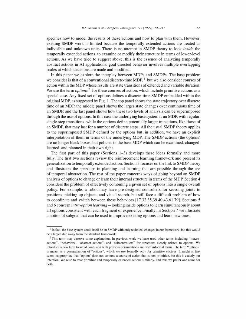
we consider is that of a conventional discrete-time MDP, 1 but we also consider courses ofaction within theMDP whose results are state transitions of extended and variable duration.We use the term options 2 for these courses of action, which include primitive actions as aspecial case. Any fixed set of options defines a discrete-time SMDP embedded within theoriginal MDP, as suggested by Fig. 1. The top panel shows the state trajectory over discretetime of an MDP, the middle panel shows the larger state changes over continuous time ofan SMDP, and the last panel shows how these two levels of analysis can be superimposedthrough the use of options. In this case the underlying base system is an MDP, with regular,single-step transitions, while the options define potentially larger transitions, like those ofan SMDP, that may last for a number of discrete steps. All the usual SMDP theory appliesto the superimposed SMDP defined by the options but, in addition, we have an explicitinterpretation of them in terms of the underlying MDP. The SMDP actions (the options)are no longer black boxes, but policies in the base MDP which can be examined, changed,learned, and planned in their own right.The first part of this paper (Sections 1–3) develops these ideas formally and more

fully. The first two sections review the reinforcement learning framework and present itsgeneralization to temporally extended action. Section 3 focuses on the link to SMDP theoryand illustrates the speedups in planning and learning that are possible through the useof temporal abstraction. The rest of the paper concerns ways of going beyond an SMDPanalysis of options to change or learn their internal structure in terms of the MDP. Section 4considers the problem of effectively combining a given set of options into a single overallpolicy. For example, a robot may have pre-designed controllers for servoing joints topositions, picking up objects, and visual search, but still face a difficult problem of howto coordinate and switch between these behaviors [17,32,35,39,40,43,61,79]. Sections 5and 6 concern intra-option learning—looking inside options to learn simultaneously aboutall options consistent with each fragment of experience. Finally, in Section 7 we illustratea notion of subgoal that can be used to improve existing options and learn new ones.

1 In fact, the base system could itself be an SMDP with only technical changes in our framework, but this wouldbe a larger step away from the standard framework.2 This term may deserve some explanation. In previous work we have used other terms including “macro-

actions”, “behaviors”, “abstract actions”, and “subcontrollers” for structures closely related to options. Weintroduce a new term to avoid confusion with previous formulations and with informal terms. The term “options”is meant as a generalization of “actions”, which we use formally only for primitive choices. It might at firstseem inappropriate that “option” does not connote a course of action that is non-primitive, but this is exactly ourintention. We wish to treat primitive and temporally extended actions similarly, and thus we prefer one name forboth.


Fig. 1. The state trajectory of an MDP is made up of small, discrete-time transitions, whereas that of an SMDPcomprises larger, continuous-time transitions. Options enable an MDP trajectory to be analyzed in either way.

1. The reinforcement learning (MDP) framework

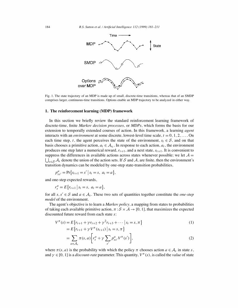
In this section we briefly review the standard reinforcement learning framework ofdiscrete-time, finite Markov decision processes, or MDPs, which forms the basis for ourextension to temporally extended courses of action. In this framework, a learning agentinteracts with an environment at some discrete, lowest-level time scale, t = 0,1,2, . . . . Oneach time step, t , the agent perceives the state of the environment, st " S , and on thatbasis chooses a primitive action, at " Ast . In response to each action, at , the environmentproduces one step later a numerical reward, rt+1, and a next state, st+1. It is convenient tosuppress the differences in available actions across states whenever possible; we let A =⋃

s"S As denote the union of the action sets. If S andA, are finite, then the environment’stransition dynamics can be modeled by one-step state-transition probabilities,

pass # = Pr

{st+1 = s# ∣∣ st = s, at = a

},

and one-step expected rewards,

ras = E

{rt+1

∣∣ st = s, at = a},

for all s, s# " S and a " As . These two sets of quantities together constitute the one-stepmodel of the environment.The agent’s objective is to learn aMarkov policy, a mapping from states to probabilities

of taking each available primitive action, ! :S $A % [0,1], that maximizes the expecteddiscounted future reward from each state s:

V ! (s) = E{rt+1 + " rt+2 + " 2rt+3 + · · ·

∣∣ st = s,!}

(1)= E

{rt+1 + "V ! (st+1)

∣∣ st = s,!}

=∑

a"As

!(s, a)

[ras + "

∑

s #pa

ss #V! (s#)

], (2)

where !(s, a) is the probability with which the policy ! chooses action a " As in state s,and " " [0,1] is a discount-rate parameter. This quantity, V ! (s), is called the value of state


s under policy ! , and V ! is called the state-value function for ! . The optimal state-valuefunction gives the value of each state under an optimal policy:

V !(s) =max!

V ! (s) (3)

= maxa"As

E{rt+1 + "V !(st+1)

∣∣ st = s, at = a}

= maxa"As

[ras + "

∑

s #pa

ss #V!(s#)

]. (4)

Any policy that achieves the maximum in (3) is by definition an optimal policy. Thus, givenV !, an optimal policy is easily formed by choosing in each state s any action that achievesthe maximum in (4). Planning in reinforcement learning refers to the use of models of theenvironment to compute value functions and thereby to optimize or improve policies. Par-ticularly useful in this regard are Bellman equations, such as (2) and (4), which recursivelyrelate value functions to themselves. If we treat the values, V ! (s) or V !(s), as unknowns,then a set of Bellman equations, for all s " S , forms a system of equations whose uniquesolution is in fact V ! or V ! as given by (1) or (3). This fact is key to the way in which alltemporal-difference and dynamic programming methods estimate value functions.There are similar value functions and Bellman equations for state-action pairs, rather

than for states, which are particularly important for learning methods. The value of takingaction a in state s under policy ! , denoted Q! (s, a), is the expected discounted futurereward starting in s, taking a, and henceforth following ! :

Q! (s, a) = E{rt+1 + " rt+2 + " 2rt+3 + · · ·

∣∣ st = s, at = a,!}

= ras + "

∑

s #pa

ss #V! (s#)

= ras + "

∑

s #pa

ss #∑

a#!(s#, a#)Q! (s#, a#).

This is known as the action-value function for policy ! . The optimal action-value functionis

Q!(s, a) =max!

Q! (s, a)

= ras + "

∑

s #pa

ss #maxa#

Q!(s#, a#).

Finally, many tasks are episodic in nature, involving repeated trials, or episodes, eachending with a reset to a standard state or state distribution. Episodic tasks include a specialterminal state; arriving in this state terminates the current episode. The set of regular statesplus the terminal state (if there is one) is denoted S+. Thus, the s# in pa

ss # in general rangesover the set S+ rather than just S as stated earlier. In an episodic task, values are defined bythe expected cumulative reward up until termination rather than over the infinite future (or,equivalently, we can consider the terminal state to transition to itself forever with a rewardof zero). There are also undiscounted average-reward formulations, but for simplicity wedo not consider them here. For more details and background on reinforcement learningsee [72].


2. Options

As mentioned earlier, we use the term options for our generalization of primitive actionsto include temporally extended courses of action. Options consist of three components: apolicy ! :S $ A % [0,1], a termination condition # :S+ % [0,1], and an initiation setI & S . An option 'I,!,#( is available in state st if and only if st " I . If the option istaken, then actions are selected according to ! until the option terminates stochasticallyaccording to # . In particular, a Markov option executes as follows. First, the next actionat is selected according to probability distribution !(st , ·). The environment then makes atransition to state st+1, where the option either terminates, with probability #(st+1), or elsecontinues, determining at+1 according to !(st+1, ·), possibly terminating in st+2 accordingto #(st+2), and so on. 3 When the option terminates, the agent has the opportunity to selectanother option. For example, an option named open-the-doormight consist of a policyfor reaching, grasping and turning the door knob, a termination condition for recognizingthat the door has been opened, and an initiation set restricting consideration of open-the-door to states in which a door is present. In episodic tasks, termination of an episodealso terminates the current option (i.e., # maps the terminal state to 1 in all options).The initiation set and termination condition of an option together restrict its range of

application in a potentially useful way. In particular, they limit the range over which theoption’s policy needs to be defined. For example, a handcrafted policy ! for a mobile robotto dock with its battery charger might be defined only for states I in which the batterycharger is within sight. The termination condition # could be defined to be 1 outsideof I and when the robot is successfully docked. A subpolicy for servoing a robot armto a particular joint configuration could similarly have a set of allowed starting states, acontroller to be applied to them, and a termination condition indicating that either the targetconfiguration has been reached within some tolerance or that some unexpected event hastaken the subpolicy outside its domain of application. For Markov options it is natural toassume that all states where an option might continue are also states where the option mightbe taken (i.e., that {s: #(s) < 1} & I). In this case, ! need only be defined over I ratherthan over all of S .Sometimes it is useful for options to “timeout”, to terminate after some period of time

has elapsed even if they have failed to reach any particular state. This is not possiblewith Markov options because their termination decisions are made solely on the basisof the current state, not on how long the option has been executing. To handle this andother cases of interest we allow semi-Markov options, in which policies and terminationconditions may make their choices dependent on all prior events since the option wasinitiated. In general, an option is initiated at some time, say t , determines the actionsselected for some number of steps, say k, and then terminates in st+k . At each intermediatetime $, t ! $ < t + k, the decisions of a Markov option may depend only on s$ , whereasthe decisions of a semi-Markov option may depend on the entire preceding sequencest , at , rt+1, st+1, at+1, . . . , r$ , s$ , but not on events prior to st (or after s$ ). We call thissequence the history from t to $ and denote it by ht$ . We denote the set of all histories

3 The termination condition # plays a role similar to the # in #-models [71], but with an opposite sense. Thatis, #(s) in this paper corresponds to 1 #(s) in [71].


by % . In semi-Markov options, the policy and termination condition are functions ofpossible histories, that is, they are ! :% $ A % [0,1] and # :% % [0,1]. Semi-Markovoptions also arise if options use a more detailed state representation than is availableto the policy that selects the options, as in hierarchical abstract machines [52,53] andMAXQ [16]. Finally, note that hierarchical structures, such as options that select otheroptions, can also give rise to higher-level options that are semi-Markov (even if all thelower-level options are Markov). Semi-Markov options include a very general range ofpossibilities.Given a set of options, their initiation sets implicitly define a set of available options

Os for each state s " S . These Os are much like the sets of available actions, As . We canunify these two kinds of sets by noting that actions can be considered a special case ofoptions. Each action a corresponds to an option that is available whenever a is available(I = {s: a " As}), that always lasts exactly one step (#(s) = 1,)s " S), and that selectsa everywhere (!(s, a) = 1,)s " I). Thus, we can consider the agent’s choice at each timeto be entirely among options, some of which persist for a single time step, others of whichare temporally extended. The former we refer to as single-step or primitive options and thelatter as multi-step options. Just as in the case of actions, it is convenient to suppress thedifferences in available options across states. We let O = ⋃

s"S Os denote the set of allavailable options.Our definition of options is crafted to make them as much like actions as possible while

adding the possibility that they are temporally extended. Because options terminate in awell defined way, we can consider sequences of them in much the same way as we considersequences of actions. We can also consider policies that select options instead of actions,and we can model the consequences of selecting an option much as we model the resultsof an action. Let us consider each of these in turn.Given any two options a and b, we can consider taking them in sequence, that is, we

can consider first taking a until it terminates, and then b until it terminates (or omitting baltogether if a terminates in a state outside of b’s initiation set). We say that the two optionsare composed to yield a new option, denoted ab, corresponding to this way of behaving.The composition of two Markov options will in general be semi-Markov, not Markov,because actions are chosen differently before and after the first option terminates. Thecomposition of two semi-Markov options is always another semi-Markov option. Becauseactions are special cases of options, we can also compose them to produce a deterministicaction sequence, in other words, a classical macro-operator.More interesting for our purposes are policies over options. When initiated in a state st ,

the Markov policy over options µ :S $O % [0,1] selects an option o " Ost according toprobability distribution µ(st , ·). The option o is then taken in st , determining actions untilit terminates in st+k , at which time a new option is selected, according to µ(st+k, ·), andso on. In this way a policy over options, µ, determines a conventional policy over actions,or flat policy, ! = flat(µ). Henceforth we use the unqualified term policy for policies overoptions, which include flat policies as a special case. Note that even if a policy is Markovand all of the options it selects are Markov, the corresponding flat policy is unlikely to beMarkov if any of the options are multi-step (temporally extended). The action selected bythe flat policy in state s$ depends not just on s$ but on the option being followed at thattime, and this depends stochastically on the entire history ht$ since the policy was initiated


at time t . 4 By analogy to semi-Markov options, we call policies that depend on historiesin this way semi-Markov policies. Note that semi-Markov policies are more specializedthan nonstationary policies. Whereas nonstationary policies may depend arbitrarily on allpreceding events, semi-Markov policies may depend only on events back to some particulartime. Their decisions must be determined solely by the event subsequence from that timeto the present, independent of the events preceding that time.These ideas lead to natural generalizations of the conventional value functions for a

given policy. We define the value of a state s " S under a semi-Markov flat policy ! as theexpected return given that ! is initiated in s:

V ! (s)def= E

{rt+1 + " rt+2 + " 2rt+3 + · · ·

∣∣E(!, s, t)},

where E(!, s, t) denotes the event of ! being initiated in s at time t . The value of astate under a general policy µ can then be defined as the value of the state under thecorresponding flat policy: V µ(s)=defV flat(µ)(s), for all s " S . Action-value functionsgeneralize to option-value functions. We define Qµ(s, o), the value of taking option o

in state s " I under policy µ, as

Qµ(s, o)def= E

{rt+1 + " rt+2 + " 2rt+3 + · · ·

∣∣E(oµ, s, t)}, (5)

where oµ, the composition of o and µ, denotes the semi-Markov policy that first followso until it terminates and then starts choosing according to µ in the resultant state. Forsemi-Markov options, it is useful to define E(o,h, t), the event of o continuing from h

at time t , where h is a history ending with st . In continuing, actions are selected as if thehistory had preceded st . That is, at is selected according to o(h, ·), and o terminates at t +1with probability #(hat rt+1st+1); if o does not terminate, then at+1 is selected according too(hatrt+1st+1, ·), and so on. With this definition, (5) also holds where s is a history ratherthan a state.This completes our generalization to temporal abstraction of the concept of value

functions for a given policy. In the next section we similarly generalize the concept ofoptimal value functions.

3. SMDP (option-to-option) methods

Options are closely related to the actions in a special kind of decision problem known asa semi-Markov decision process, or SMDP (e.g., see [58]). In fact, any MDP with a fixedset of options is an SMDP, as we state formally below. Although this fact follows moreor less immediately from definitions, we present it as a theorem to highlight it and stateexplicitly its conditions and consequences:

Theorem 1 (MDP+Options= SMDP). For any MDP, and any set of options defined onthat MDP, the decision process that selects only among those options, executing each totermination, is an SMDP.

4 For example, the options for picking up an object and putting down an object may specify different actions inthe same intermediate state; which action is taken depends on which option is being followed.


Proof (Sketch). An SMDP consists of(1) a set of states,(2) a set of actions,(3) for each pair of state and action, an expected cumulative discounted reward, and(4) a well-defined joint distribution of the next state and transit time.

In our case, the set of states is S , and the set of actions is the set of options. The expectedreward and the next-state and transit-time distributions are defined for each state andoption by the MDP and by the option’s policy and termination condition, ! and # . Theseexpectations and distributions are well defined because MDPs are Markov and the optionsare semi-Markov; thus the next state, reward, and time are dependent only on the optionand the state in which it was initiated. The transit times of options are always discrete, butthis is simply a special case of the arbitrary real intervals permitted in SMDPs. !

This relationship among MDPs, options, and SMDPs provides a basis for the theory ofplanning and learning methods with options. In later sections we discuss the limitationsof this theory due to its treatment of options as indivisible units without internal structure,but in this section we focus on establishing the benefits and assurances that it provides. Weestablish theoretical foundations and then survey SMDP methods for planning and learningwith options. Although our formalism is slightly different, these results are in essence takenor adapted from prior work (including classical SMDP work and [5,44,52–57,65–68,71,74,75]). A result very similar to Theorem 1 was proved in detail by Parr [52]. In Sections 4–7we present new methods that improve over SMDP methods.Planning with options requires a model of their consequences. Fortunately, the

appropriate form of model for options, analogous to the ras and pa

ss # defined earlier foractions, is known from existing SMDP theory. For each state in which an option may bestarted, this kind of model predicts the state in which the option will terminate and the totalreward received along the way. These quantities are discounted in a particular way. For anyoption o, let E(o, s, t) denote the event of o being initiated in state s at time t . Then thereward part of the model of o for any state s " S is

ros = E

{rt+1 + " rt+2 + · · · + " k 1rt+k

∣∣E(o, s, t)}, (6)

where t + k is the random time at which o terminates. The state-prediction part of themodel of o for state s is

poss # =

*∑

k=1p(s#, k)" k, (7)

for all s# " S , where p(s#, k) is the probability that the option terminates in s# after k steps.Thus, po

ss # is a combination of the likelihood that s# is the state in which o terminatestogether with a measure of how delayed that outcome is relative to " . We call this kind ofmodel a multi-time model [54,55] because it describes the outcome of an option not at asingle time but at potentially many different times, appropriately combined. 5

5 Note that this definition of state predictions for options differs slightly from that given earlier for actions.Under the new definition, the model of transition from state s to s# for an action a is not simply the correspondingtransition probability, but the transition probability times " . Henceforth we use the new definition given by (7).


Using multi-time models we can write Bellman equations for general policies andoptions. For any Markov policy µ, the state-value function can be written

V µ(s) = E{rt+1 + · · · + " k 1rt+k + " kV µ(st+k)

∣∣E(µ, s, t)}

(where k is the duration of the first option selected by µ)

=∑

o"Os

µ(s, o)

[ros +

∑

s #po

ss #Vµ(s#)

], (8)

which is a Bellman equation analogous to (2). The corresponding Bellman equation for thevalue of an option o in state s " I is

Qµ(s, o) = E{rt+1 + · · · + " k 1rt+k + " kV µ(st+k)

∣∣E(o, s, t)},

= E

{rt+1 + · · · + " k 1rt+k

+ " k∑

o#"Os

µ(st+k, o#)Qµ(st+k, o

#)∣∣∣E(o, s, t)

}

= ros +

∑

s #po

ss #∑

o#"Os#

µ(s#, o#)Qµ(s#, o#). (9)

Note that all these equations specialize to those given earlier in the special case in which µ

is a conventional policy and o is a conventional action. Also note that Qµ(s, o) = V oµ(s).Finally, there are generalizations of optimal value functions and optimal Bellman

equations to options and to policies over options. Of course the conventional optimal valuefunctions V ! andQ! are not affected by the introduction of options; one can ultimately dojust as well with primitive actions as one can with options. Nevertheless, it is interestingto know how well one can do with a restricted set of options that does not include all theactions. For example, in planning one might first consider only high-level options in orderto find an approximate plan quickly. Let us denote the restricted set of options by O andthe set of all policies selecting only from options in O by &(O). Then the optimal valuefunction given that we can select only from O is

V !O(s)

def= maxµ"&(O)

V µ(s)

= maxo"Os

E{rt+1 + · · · + " k 1rt+k + " kV !

O(st+k)∣∣E(o, s, t)

}

(where k is the duration of o when taken in s)

= maxo"Os

[ros +

∑

s #po

ss #V!O(s#)

](10)

= maxo"Os

E{r + " kV !

O(s#)∣∣E(o, s)

}, (11)

where E(o, s) denotes option o being initiated in state s. Conditional on this event are theusual random variables: s# is the state in which o terminates, r is the cumulative discountedreward along the way, and k is the number of time steps elapsing between s and s#. Thevalue functions and Bellman equations for optimal option values are


Q!O(s, o)

def= maxµ"&(O)

Qµ(s, o)

= E{rt+1 + · · · + " k 1rt+k + " kV !

O(st+k)∣∣E(o, s, t)

}

(where k is the duration of o from s)

= E{rt+1 + · · · + " k 1rt+k + " k max

o#"Ost+k

Q!O(st+k, o

#)∣∣∣E(o, s, t)

},

= ros +

∑

s #po

ss # maxo#"Os#

Q!O(s#, o#)

= E{r + " k max

o#"Os#Q!

O(s#, o#)∣∣∣E(o, s)

}, (12)

where r , k, and s# are again the reward, number of steps, and next state due to takingo " Os .Given a set of options, O, a corresponding optimal policy, denoted µ!

O , is any policythat achieves V !

O , i.e., for which V µ!O (s) = V !

O(s) in all states s " S . If V !O and models of

the options are known, then optimal policies can be formed by choosing in any propositionamong the maximizing options in (10) or (11). Or, if Q!

O is known, then optimal policiescan be found without a model by choosing in each state s in any proportion among theoptions o for which Q!

O(s, o) =maxo# Q!O(s, o#). In this way, computing approximations

to V !O or Q

!O become key goals of planning and learning methods with options.

3.1. SMDP planning

With these definitions, an MDP together with the set of options O formally comprisesan SMDP, and standard SMDP methods and results apply. Each of the Bellman equationsfor options, (8), (9), (10), and (12), defines a system of equations whose unique solutionis the corresponding value function. These Bellman equations can be used as update rulesin dynamic-programming-like planning methods for finding the value functions. Typically,solution methods for this problem maintain an approximation of V !

O(s) orQ!O(s, o) for all

states s " S and all options o " Os . For example, synchronous value iteration (SVI) withoptions starts with an arbitrary approximation V0 to V !

O and then computes a sequence ofnew approximations {Vk} by

Vk(s) = maxo"Os

[ros +

∑

s #"Spo

ss #Vk 1(s#)]

(13)

for all s " S . The option-value form of SVI starts with an arbitrary approximation Q0 toQ!

O and then computes a sequence of new approximations {Qk} by

Qk(s, o) = ros +

∑

s #"Spo

ss # maxo#"Os#

Qk 1(s#, o#)

for all s " S and o " Os . Note that these algorithms reduce to the conventional valueiteration algorithms in the special case that O = A. Standard results from SMDP theoryguarantee that these processes converge for general semi-Markov options: limk%* Vk =V !O and limk%* Qk = Q!

O , for any O.


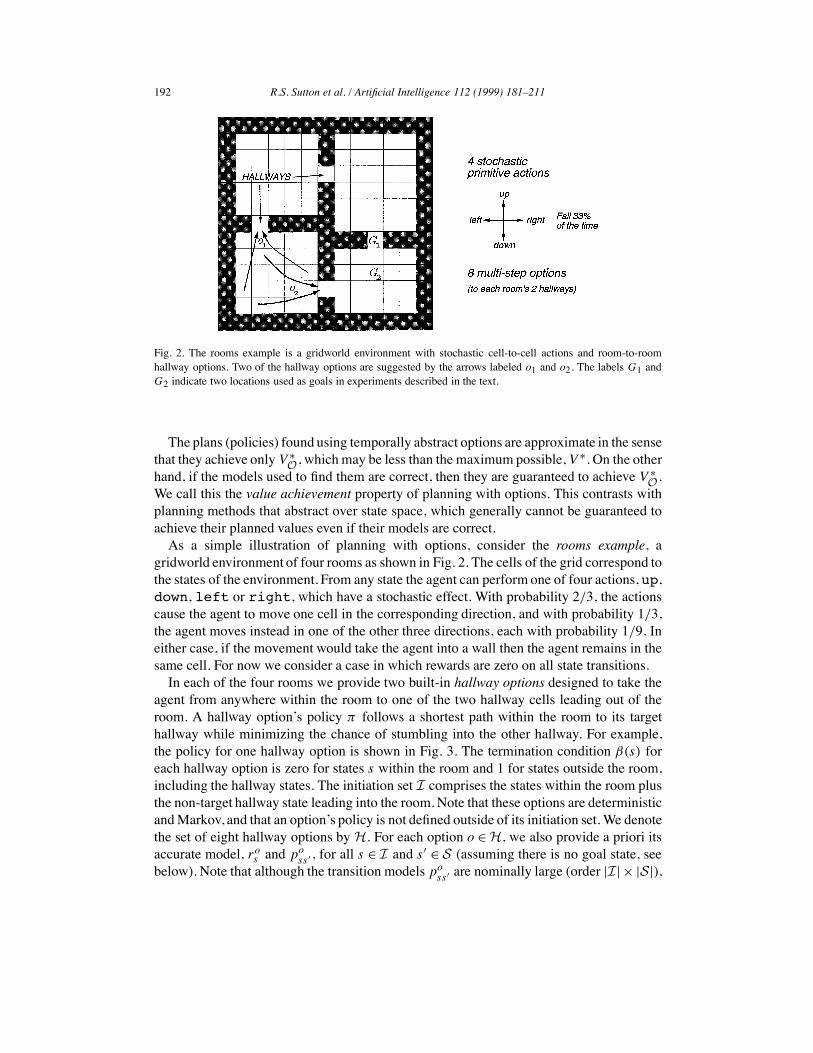
Fig. 2. The rooms example is a gridworld environment with stochastic cell-to-cell actions and room-to-roomhallway options. Two of the hallway options are suggested by the arrows labeled o1 and o2. The labels G1 andG2 indicate two locations used as goals in experiments described in the text.

The plans (policies) found using temporally abstract options are approximate in the sensethat they achieve only V !

O, which may be less than the maximum possible, V!. On the other

hand, if the models used to find them are correct, then they are guaranteed to achieve V !O .

We call this the value achievement property of planning with options. This contrasts withplanning methods that abstract over state space, which generally cannot be guaranteed toachieve their planned values even if their models are correct.As a simple illustration of planning with options, consider the rooms example, a

gridworld environment of four rooms as shown in Fig. 2. The cells of the grid correspond tothe states of the environment. From any state the agent can perform one of four actions, up,down, left or right, which have a stochastic effect. With probability 2/3, the actionscause the agent to move one cell in the corresponding direction, and with probability 1/3,the agent moves instead in one of the other three directions, each with probability 1/9. Ineither case, if the movement would take the agent into a wall then the agent remains in thesame cell. For now we consider a case in which rewards are zero on all state transitions.In each of the four rooms we provide two built-in hallway options designed to take the

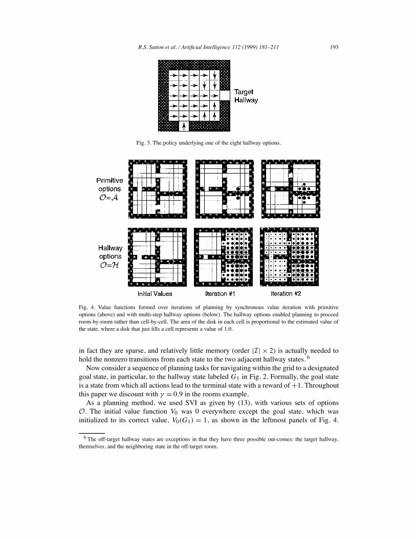
agent from anywhere within the room to one of the two hallway cells leading out of theroom. A hallway option’s policy ! follows a shortest path within the room to its targethallway while minimizing the chance of stumbling into the other hallway. For example,the policy for one hallway option is shown in Fig. 3. The termination condition #(s) foreach hallway option is zero for states s within the room and 1 for states outside the room,including the hallway states. The initiation set I comprises the states within the room plusthe non-target hallway state leading into the room. Note that these options are deterministicandMarkov, and that an option’s policy is not defined outside of its initiation set. We denotethe set of eight hallway options by H. For each option o " H, we also provide a priori itsaccurate model, ro

s and poss # , for all s " I and s# " S (assuming there is no goal state, see

below). Note that although the transition models poss # are nominally large (order |I|$ |S|),


Fig. 3. The policy underlying one of the eight hallway options.

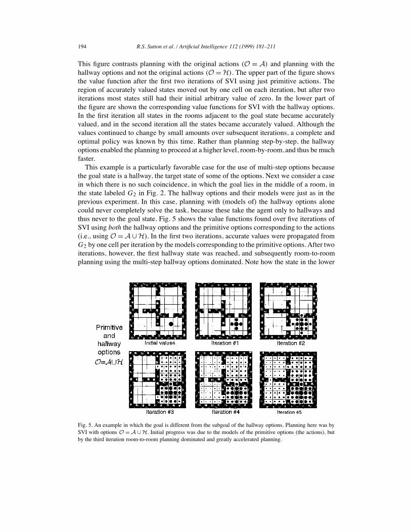
Fig. 4. Value functions formed over iterations of planning by synchronous value iteration with primitiveoptions (above) and with multi-step hallway options (below). The hallway options enabled planning to proceedroom-by-room rather than cell-by-cell. The area of the disk in each cell is proportional to the estimated value ofthe state, where a disk that just fills a cell represents a value of 1.0.

in fact they are sparse, and relatively little memory (order |I| $ 2) is actually needed tohold the nonzero transitions from each state to the two adjacent hallway states. 6Now consider a sequence of planning tasks for navigating within the grid to a designated

goal state, in particular, to the hallway state labeled G1 in Fig. 2. Formally, the goal stateis a state from which all actions lead to the terminal state with a reward of +1. Throughoutthis paper we discount with " = 0.9 in the rooms example.As a planning method, we used SVI as given by (13), with various sets of options

O. The initial value function V0 was 0 everywhere except the goal state, which wasinitialized to its correct value, V0(G1) = 1, as shown in the leftmost panels of Fig. 4.

6 The off-target hallway states are exceptions in that they have three possible out-comes: the target hallway,themselves, and the neighboring state in the off-target room.


This figure contrasts planning with the original actions (O = A) and planning with thehallway options and not the original actions (O = H). The upper part of the figure showsthe value function after the first two iterations of SVI using just primitive actions. Theregion of accurately valued states moved out by one cell on each iteration, but after twoiterations most states still had their initial arbitrary value of zero. In the lower part ofthe figure are shown the corresponding value functions for SVI with the hallway options.In the first iteration all states in the rooms adjacent to the goal state became accuratelyvalued, and in the second iteration all the states became accurately valued. Although thevalues continued to change by small amounts over subsequent iterations, a complete andoptimal policy was known by this time. Rather than planning step-by-step, the hallwayoptions enabled the planning to proceed at a higher level, room-by-room, and thus be muchfaster.This example is a particularly favorable case for the use of multi-step options because

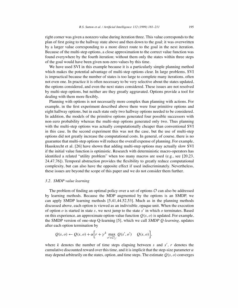
the goal state is a hallway, the target state of some of the options. Next we consider a casein which there is no such coincidence, in which the goal lies in the middle of a room, inthe state labeled G2 in Fig. 2. The hallway options and their models were just as in theprevious experiment. In this case, planning with (models of) the hallway options alonecould never completely solve the task, because these take the agent only to hallways andthus never to the goal state. Fig. 5 shows the value functions found over five iterations ofSVI using both the hallway options and the primitive options corresponding to the actions(i.e., using O = A + H). In the first two iterations, accurate values were propagated fromG2 by one cell per iteration by the models corresponding to the primitive options. After twoiterations, however, the first hallway state was reached, and subsequently room-to-roomplanning using the multi-step hallway options dominated. Note how the state in the lower

Fig. 5. An example in which the goal is different from the subgoal of the hallway options. Planning here was bySVI with options O = A +H. Initial progress was due to the models of the primitive options (the actions), butby the third iteration room-to-room planning dominated and greatly accelerated planning.


right corner was given a nonzero value during iteration three. This value corresponds to theplan of first going to the hallway state above and then down to the goal; it was overwrittenby a larger value corresponding to a more direct route to the goal in the next iteration.Because of the multi-step options, a close approximation to the correct value function wasfound everywhere by the fourth iteration; without them only the states within three stepsof the goal would have been given non-zero values by this time.We have used SVI in this example because it is a particularly simple planning method

which makes the potential advantage of multi-step options clear. In large problems, SVIis impractical because the number of states is too large to complete many iterations, oftennot even one. In practice it is often necessary to be very selective about the states updated,the options considered, and even the next states considered. These issues are not resolvedby multi-step options, but neither are they greatly aggravated. Options provide a tool fordealing with them more flexibly.Planning with options is not necessarily more complex than planning with actions. For

example, in the first experiment described above there were four primitive options andeight hallway options, but in each state only two hallway options needed to be considered.In addition, the models of the primitive options generated four possible successors withnon-zero probability whereas the multi-step options generated only two. Thus planningwith the multi-step options was actually computationally cheaper than conventional SVIin this case. In the second experiment this was not the case, but the use of multi-stepoptions did not greatly increase the computational costs. In general, of course, there is noguarantee that multi-step options will reduce the overall expense of planning. For example,Hauskrecht et al. [26] have shown that adding multi-step options may actually slow SVIif the initial value function is optimistic. Research with deterministic macro-operators hasidentified a related “utility problem” when too many macros are used (e.g., see [20,23,24,47,76]). Temporal abstraction provides the flexibility to greatly reduce computationalcomplexity, but can also have the opposite effect if used indiscriminately. Nevertheless,these issues are beyond the scope of this paper and we do not consider them further.

3.2. SMDP value learning

The problem of finding an optimal policy over a set of options O can also be addressedby learning methods. Because the MDP augmented by the options is an SMDP, wecan apply SMDP learning methods [5,41,44,52,53]. Much as in the planning methodsdiscussed above, each option is viewed as an indivisible, opaque unit. When the executionof option o is started in state s, we next jump to the state s# in which o terminates. Basedon this experience, an approximate option-value functionQ(s, o) is updated. For example,the SMDP version of one-step Q-learning [5], which we call SMDP Q-learning, updatesafter each option termination by

Q(s, o) , Q(s, o) + '[r + " k max

o#"Os#Q(s#, o#) Q(s, o)

],

where k denotes the number of time steps elapsing between s and s#, r denotes thecumulative discounted reward over this time, and it is implicit that the step-size parameter 'may depend arbitrarily on the states, option, and time steps. The estimateQ(s, o) converges


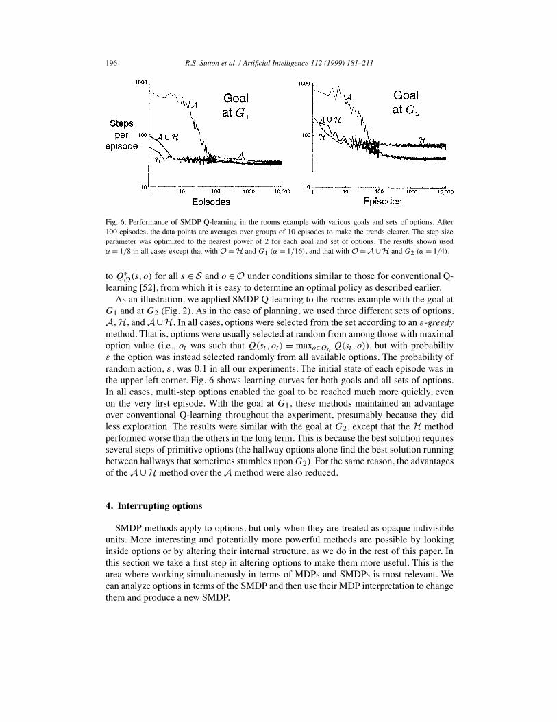
Fig. 6. Performance of SMDP Q-learning in the rooms example with various goals and sets of options. After100 episodes, the data points are averages over groups of 10 episodes to make the trends clearer. The step sizeparameter was optimized to the nearest power of 2 for each goal and set of options. The results shown used' = 1/8 in all cases except that with O = H and G1 (' = 1/16), and that with O =A +H and G2 (' = 1/4).

to Q!O(s, o) for all s " S and o " O under conditions similar to those for conventional Q-

learning [52], from which it is easy to determine an optimal policy as described earlier.As an illustration, we applied SMDP Q-learning to the rooms example with the goal at

G1 and at G2 (Fig. 2). As in the case of planning, we used three different sets of options,A,H, andA+H. In all cases, options were selected from the set according to an (-greedymethod. That is, options were usually selected at random from among those with maximaloption value (i.e., ot was such that Q(st , ot ) = maxo"Ost

Q(st , o)), but with probability( the option was instead selected randomly from all available options. The probability ofrandom action, (, was 0.1 in all our experiments. The initial state of each episode was inthe upper-left corner. Fig. 6 shows learning curves for both goals and all sets of options.In all cases, multi-step options enabled the goal to be reached much more quickly, evenon the very first episode. With the goal at G1, these methods maintained an advantageover conventional Q-learning throughout the experiment, presumably because they didless exploration. The results were similar with the goal at G2, except that the H methodperformed worse than the others in the long term. This is because the best solution requiresseveral steps of primitive options (the hallway options alone find the best solution runningbetween hallways that sometimes stumbles uponG2). For the same reason, the advantagesof the A+H method over the A method were also reduced.

4. Interrupting options

SMDP methods apply to options, but only when they are treated as opaque indivisibleunits. More interesting and potentially more powerful methods are possible by lookinginside options or by altering their internal structure, as we do in the rest of this paper. Inthis section we take a first step in altering options to make them more useful. This is thearea where working simultaneously in terms of MDPs and SMDPs is most relevant. Wecan analyze options in terms of the SMDP and then use their MDP interpretation to changethem and produce a new SMDP.


In particular, in this section we consider interrupting options before they wouldterminate naturally according to their termination conditions. Note that treating optionsas indivisible units, as SMDP methods do, is limiting in an unnecessary way. Once anoption has been selected, such methods require that its policy be followed until the optionterminates. Suppose we have determined the option-value function Qµ(s, o) for somepolicy µ and for all state-option pairs s, o that could be encountered while followingµ. This function tells us how well we do while following µ, committing irrevocably toeach option, but it can also be used to re-evaluate our commitment on each step. Supposeat time t we are in the midst of executing option o. If o is Markov in st , then we cancompare the value of continuing with o, which is Qµ(st , o), to the value of interrupting o

and selecting a new option according to µ, which is V µ(s) = ∑q µ(s, q)Qµ(s, q). If the

latter is more highly valued, then why not interrupt o and allow the switch? If these weresimple actions, the classical policy improvement theorem [27] would assure us that the newway of behaving is indeed better. Here we prove the generalization to semi-Markov options.The first empirical demonstration of this effect—improved performance by interruptinga temporally extended substep based on a value function found by planning at a higherlevel—may have been by Kaelbling [31]. Here we formally prove the improvement in amore general setting.In the following theorem we characterize the new way of behaving as following a

policy µ# that is the same as the original policy, µ, but over a new set of options;µ#(s, o#) = µ(s, o), for all s " S . Each new option o# is the same as the correspondingold option o except that it terminates whenever switching seems better than continuingaccording to Qµ. In other words, the termination condition # # of o# is the same as that ofo except that # #(s) = 1 if Qµ(s, o) < V µ(s). We call such a µ# an interrupted policyof µ. The theorem is slightly more general in that it does not require interruption ateach state in which it could be done. This weakens the requirement that Qµ(s, o) becompletely known. A more important generalization is that the theorem applies to semi-Markov options rather than just Markov options. This generalization may make the resultless intuitively accessible on first reading. Fortunately, the result can be read as restrictedto the Markov case simply by replacing every occurrence of “history” with “state” and setof histories,% , with set of states, S .

Theorem 2 (Interruption). For any MDP, any set of options O, and any Markov policyµ :S $ O % [0,1], define a new set of options, O#, with a one-to-one mapping betweenthe two option sets as follows: for every o = 'I,!,#( " O we define a correspondingo# = 'I,!,# #( " O#, where # # = # except that for any history h that ends in state s and inwhichQµ(h,o) < V µ(s), we may choose to set # #(h) = 1. Any histories whose terminationconditions are changed in this way are called interrupted histories. Let the interruptedpolicy µ# be such that for all s " S , and for all o# " O#, µ#(s, o#) = µ(s, o), where o is theoption in O corresponding to o#. Then(i) V µ#

(s) " V µ(s) for all s " S .(ii) If from state s " S there is a non-zero probability of encountering an interrupted

history upon initiating µ# in s, then V µ#(s) > V µ(s).


Proof. Shortly we show that, for an arbitrary start state s, executing the option given bythe interrupted policy µ# and then following policy µ thereafter is no worse than alwaysfollowing policy µ. In other words, we show that the following inequality holds:

∑

o#µ#(s, o#)

[ro#s +

∑

s #po#

ss #Vµ(s#)

]

" V µ(s) =∑

o

µ(s, o)

[ros +

∑

s #po

ss #Vµ(s#)

]. (14)

If this is true, then we can use it to expand the left-hand side, repeatedly replacing everyoccurrence of V µ(x) on the left by the corresponding

∑o# µ#(x, o#)[ro#

x +∑x # po#

xx #Vµ(x #)].

In the limit, the left-hand side becomes V µ# , proving that V µ# " V µ.To prove the inequality in (14), we note that for all s,µ#(s, o#) = µ(s, o), and show that

ro#s +

∑

s #po#

ss #Vµ(s#) " ro

s +∑

s #po

ss #Vµ(s#) (15)

as follows. Let denote the set of all interrupted histories: = {h "% : #(h) -= # #(h)}.Then,

ro#s +

∑

s #po#

ss #Vµ(s#) = E

{r + " kV µ(s#)

∣∣E(o#, s), h /"}

+ E{r + " kV µ(s#)

∣∣E(o#, s), h " }

where s#, r , and k are the next state, cumulative reward, and number of elapsed stepsfollowing option o from s, and where h is the history from s to s#. Trajectories that endbecause of encountering a history not in never encounter a history in , and thereforealso occur with the same probability and expected reward upon executing option o in states. Therefore, if we continue the trajectories that end because of encountering a history inwith option o until termination and thereafter follow policy µ, we get

E{r + " kV µ(s#)

∣∣E(o#, s), h /"}

+E{#(s#)

[r + " kV µ(s#)

] + 1 #(s#))[

r + " kQµ(h, o)] ∣∣E(o#, s), h " }

= ros +

∑

s #po

ss #Vµ(s#),

because option o is semi-Markov. This proves (14) because for all h " ,

Qµ(h,o) ! V µ(s#).

Note that strict inequality holds in (15) ifQµ(h,o) < V µ(s#) for at least one history h "that ends a trajectory generated by o# with non-zero probability. !

As one application of this result, consider the case in which µ is an optimal policyfor some given set of Markov options O. We have already discussed how we can, byplanning or learning, determine the optimal value functions V !

O and Q!O and from them

the optimal policy µ!O that achieves them. This is indeed the best that can be done without


changingO, that is, in the SMDP defined byO, but less than the best possible achievable inthe MDP, which is V ! = V !

A. But of course we typically do not wish to work directly withthe (primitive) actions A because of the computational expense. The interruption theoremgives us a way of improving over µ!

O with little additional computation by steppingoutsideO. That is, at each step we interrupt the current option and switch to any new optionthat is valued more highly according to Q!

O . Checking for such options can typically bedone at vastly less expense per time step than is involved in the combinatorial process ofcomputing Q!

O . In this sense, interruption gives us a nearly free improvement over anySMDP planning or learning method that computesQ!

O as an intermediate step.In the extreme case, we might interrupt on every step and switch to the greedy option—

the option in that state that is most highly valued according to Q!O (as in polling

execution [16]). In this case, options are never followed for more than one step, and theymight seem superfluous. However, the options still play a role in determining Q!

O , thebasis on which the greedy switches are made, and recall that multi-step options may enableQ!

O to be found much more quickly than Q! could (Section 3). Thus, even if multi-stepoptions are never actually followed for more than one step they can still provide substantialadvantages in computation and in our theoretical understanding.Fig. 7 shows a simple example. Here the task is to navigate from a start location to a

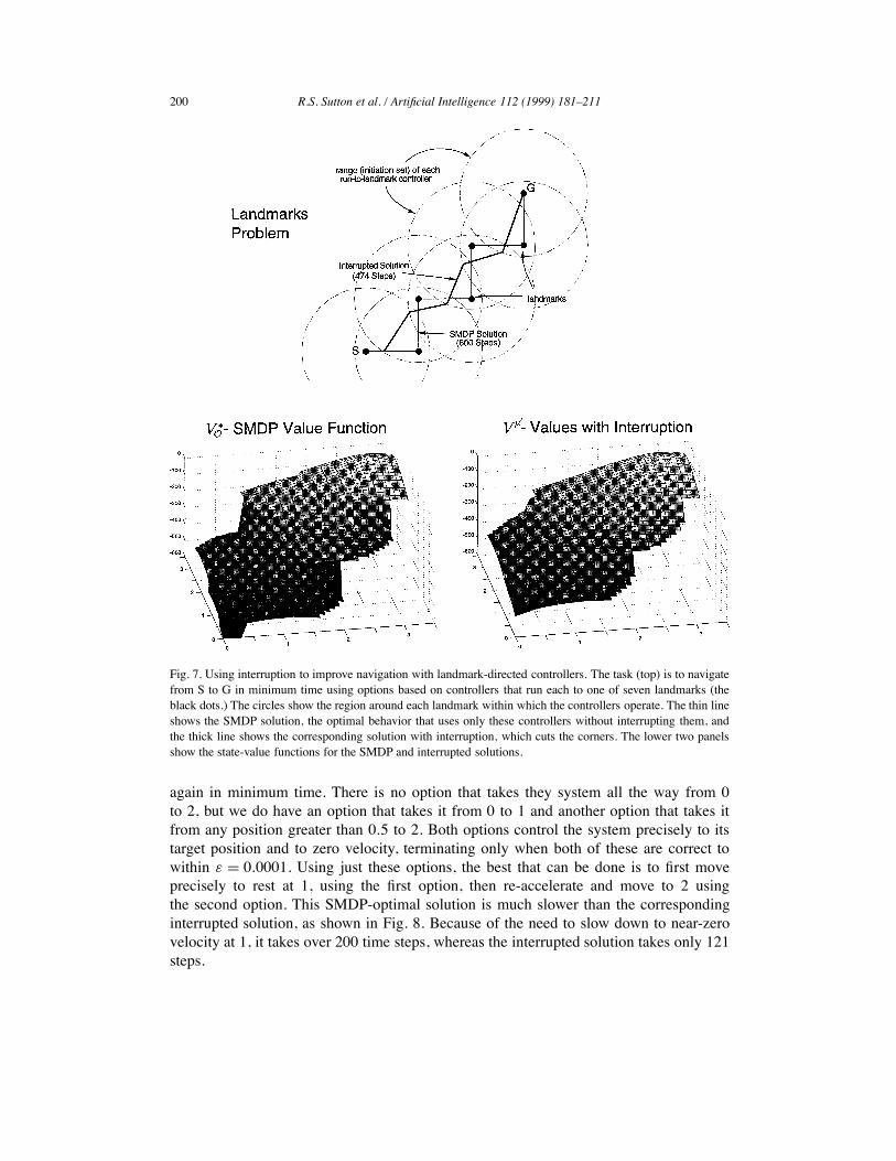
goal location within a continuous two-dimensional state space. The actions are movementsof 0.01 in any direction from the current state. Rather than work with these low-levelactions, infinite in number, we introduce seven landmark locations in the space. For eachlandmarkwe define a controller that takes us to the landmark in a direct path (cf. [48]). Eachcontroller is only applicable within a limited range of states, in this case within a certaindistance of the corresponding landmark. Each controller then defines an option: the circularregion around the controller’s landmark is the option’s initiation set, the controller itself isthe policy, and arrival at the target landmark is the termination condition.We denote the setof seven landmark options by O. Any action within 0.01 of the goal location transitions tothe terminal state, the discount rate " is 1, and the reward is 1 on all transitions, whichmakes this a minimum-time task.One of the landmarks coincides with the goal, so it is possible to reach the goal while

picking only from O. The optimal policy within O runs from landmark to landmark, asshown by the thin line in the upper panel of Fig. 7. This is the optimal solution to theSMDP defined by O and is indeed the best that one can do while picking only from theseoptions. But of course one can do better if the options are not followed all the way to eachlandmark. The trajectory shown by the thick line in Fig. 7 cuts the corners and is shorter.This is the interrupted policy with respect to the SMDP-optimal policy. The interruptedpolicy takes 474 steps from start to goal which, while not as good as the optimal policy inprimitive actions (425 steps), is much better, for nominal additional cost, than the SMDP-optimal policy, which takes 600 steps. The state-value functions, V µ = V !

O and V µ# for thetwo policies are shown in the lower part of Fig. 7. Note how the values for the interruptedpolicy are everywhere greater than the values of the original policy. A related but largerapplication of the interruption idea to mission planning for uninhabited air vehicles is givenin [75].Fig. 8 shows results for an example using controllers/options with dynamics. The task

here is to move a mass along one dimension from rest at position 0 to rest at position 2,


Fig. 7. Using interruption to improve navigation with landmark-directed controllers. The task (top) is to navigatefrom S to G in minimum time using options based on controllers that run each to one of seven landmarks (theblack dots.) The circles show the region around each landmark within which the controllers operate. The thin lineshows the SMDP solution, the optimal behavior that uses only these controllers without interrupting them, andthe thick line shows the corresponding solution with interruption, which cuts the corners. The lower two panelsshow the state-value functions for the SMDP and interrupted solutions.

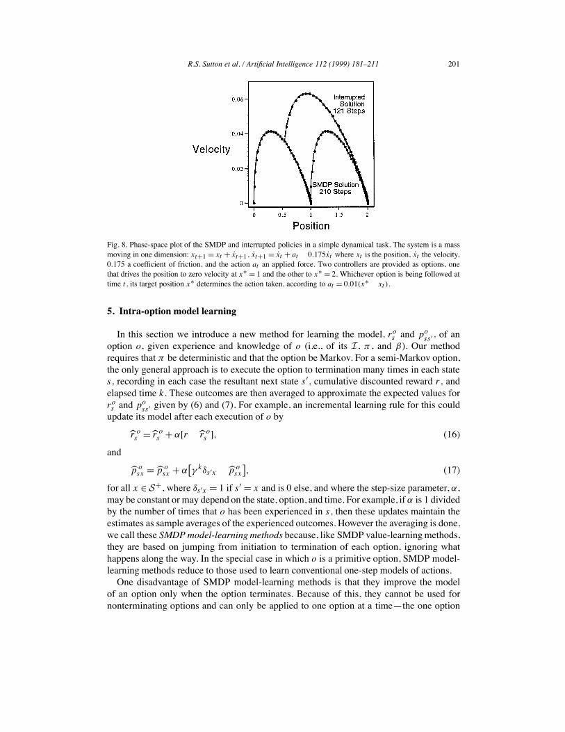
again in minimum time. There is no option that takes they system all the way from 0to 2, but we do have an option that takes it from 0 to 1 and another option that takes itfrom any position greater than 0.5 to 2. Both options control the system precisely to itstarget position and to zero velocity, terminating only when both of these are correct towithin ( = 0.0001. Using just these options, the best that can be done is to first moveprecisely to rest at 1, using the first option, then re-accelerate and move to 2 usingthe second option. This SMDP-optimal solution is much slower than the correspondinginterrupted solution, as shown in Fig. 8. Because of the need to slow down to near-zerovelocity at 1, it takes over 200 time steps, whereas the interrupted solution takes only 121steps.


Fig. 8. Phase-space plot of the SMDP and interrupted policies in a simple dynamical task. The system is a massmoving in one dimension: xt+1 = xt + xt+1, xt+1 = xt + at 0.175xt where xt is the position, xt the velocity,0.175 a coefficient of friction, and the action at an applied force. Two controllers are provided as options, onethat drives the position to zero velocity at x! = 1 and the other to x! = 2. Whichever option is being followed attime t , its target position x! determines the action taken, according to at = 0.01(x! xt ).

5. Intra-option model learning

In this section we introduce a new method for learning the model, ros and po

ss # , of anoption o, given experience and knowledge of o (i.e., of its I , ! , and #). Our methodrequires that ! be deterministic and that the option be Markov. For a semi-Markov option,the only general approach is to execute the option to termination many times in each states, recording in each case the resultant next state s#, cumulative discounted reward r , andelapsed time k. These outcomes are then averaged to approximate the expected values forros and po

ss # given by (6) and (7). For example, an incremental learning rule for this couldupdate its model after each execution of o by

r os = r o

s + '[r r os ], (16)

and

p osx = p o

sx + '[" k)s #x p o

sx

], (17)

for all x " S+, where )s #x = 1 if s# = x and is 0 else, and where the step-size parameter, ',may be constant or may depend on the state, option, and time. For example, if ' is 1 dividedby the number of times that o has been experienced in s, then these updates maintain theestimates as sample averages of the experienced outcomes. However the averaging is done,we call these SMDP model-learningmethods because, like SMDP value-learningmethods,they are based on jumping from initiation to termination of each option, ignoring whathappens along the way. In the special case in which o is a primitive option, SMDP model-learning methods reduce to those used to learn conventional one-step models of actions.One disadvantage of SMDP model-learning methods is that they improve the model

of an option only when the option terminates. Because of this, they cannot be used fornonterminating options and can only be applied to one option at a time—the one option


that is executing at that time. For Markov options, special temporal-difference methodscan be used to learn usefully about the model of an option before the option terminates.We call these intra-optionmethods because they learn about an option from a fragment ofexperience “within” the option. Intra-option methods can even be used to learn about anoption without ever executing it, as long as some selections are made that are consistentwith the option. Intra-option methods are examples of off-policy learning methods [72]because they learn about the consequences of one policy while actually behaving accordingto another. Intra-option methods can be used to simultaneously learn models of manydifferent options from the same experience. Intra-option methods were introduced in [71],but only for a prediction problem with a single unchanging policy, not for the full controlcase we consider here and in [74].Just as there are Bellman equations for value functions, there are also Bellman equations

for models of options. Consider the intra-option learning of the model of a Markov optiono = 'I,!,#(. The correct model of o is related to itself by

ros =

∑

a"As

!(s, a)E{r + " 1 #(s#)

)ros #}

(where r and s# are the reward and next stategiven that action a is taken in state s)

=∑

a"As

!(s, a)

[ras +

∑

s #pa

ss # 1 #(s#))ros #

],

and

posx =

∑

a"As

!(s, a)"E{1 #(s#)

)po

s #x + #(s#))s #x}

=∑

a"As

!(s, a)∑

s #pa

ss #[1 #(s#)

)po

s #x + #(s#))s #x],

for all s, x " S . How can we turn these Bellman-like equations into update rules forlearning the model? First consider that action at is taken in st , and that the way it wasselected is consistent with o = 'I,!,#(, that is, that at was selected with the distribution!(st , ·). Then the Bellman equations above suggest the temporal-difference update rules

r ost

, r ost

+ '[rt+1 + " 1 #(st+1)

)r ost+1 r o

st

](18)

and

p ost x

, p ost x

+ '[" 1 #(st+1))p o

st+1x + "#(st+1))st+1x p ost x

], (19)

for all x " S+, where p oss # and r o

s are the estimates of poss # and ro

s , respectively, and ' isa positive step-size parameter. The method we call one-step intra-option model learningapplies these updates to every option consistent with every action taken, at . Of course,this is just the simplest intra-option model-learning method. Others may be possible usingeligibility traces and standard tricks for off-policy learning (as in [71]).As an illustration, consider model learning in the rooms example using SMDP and intra-

option methods. As before, we assume that the eight hallway options are given, but now we


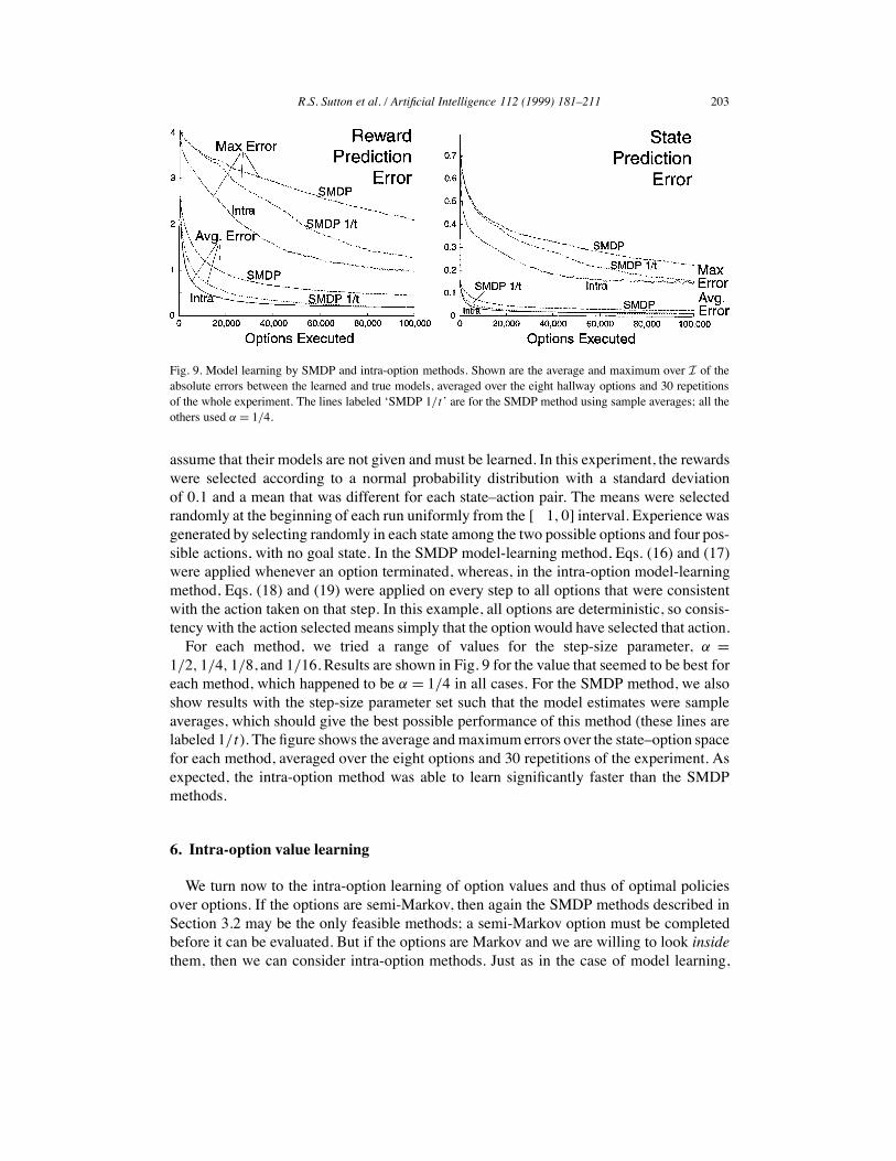
Fig. 9. Model learning by SMDP and intra-option methods. Shown are the average and maximum over I of theabsolute errors between the learned and true models, averaged over the eight hallway options and 30 repetitionsof the whole experiment. The lines labeled ‘SMDP 1/t’ are for the SMDP method using sample averages; all theothers used ' = 1/4.

assume that their models are not given and must be learned. In this experiment, the rewardswere selected according to a normal probability distribution with a standard deviationof 0.1 and a mean that was different for each state–action pair. The means were selectedrandomly at the beginning of each run uniformly from the [ 1,0] interval. Experience wasgenerated by selecting randomly in each state among the two possible options and four pos-sible actions, with no goal state. In the SMDP model-learning method, Eqs. (16) and (17)were applied whenever an option terminated, whereas, in the intra-option model-learningmethod, Eqs. (18) and (19) were applied on every step to all options that were consistentwith the action taken on that step. In this example, all options are deterministic, so consis-tency with the action selected means simply that the option would have selected that action.For each method, we tried a range of values for the step-size parameter, ' =

1/2,1/4,1/8, and 1/16. Results are shown in Fig. 9 for the value that seemed to be best foreach method, which happened to be ' = 1/4 in all cases. For the SMDP method, we alsoshow results with the step-size parameter set such that the model estimates were sampleaverages, which should give the best possible performance of this method (these lines arelabeled 1/t). The figure shows the average andmaximum errors over the state–option spacefor each method, averaged over the eight options and 30 repetitions of the experiment. Asexpected, the intra-option method was able to learn significantly faster than the SMDPmethods.

6. Intra-option value learning

We turn now to the intra-option learning of option values and thus of optimal policiesover options. If the options are semi-Markov, then again the SMDP methods described inSection 3.2 may be the only feasible methods; a semi-Markov option must be completedbefore it can be evaluated. But if the options are Markov and we are willing to look insidethem, then we can consider intra-option methods. Just as in the case of model learning,


intra-option methods for value learning are potentially more efficient than SMDP methodsbecause they extract more training examples from the same experience.For example, suppose we are learning to approximate Q!

O(s, o) and that o is Markov.Based on an execution of o from t to t +k, SMDPmethods extract a single training examplefor Q!

O(s, o). But because o is Markov, it is, in a sense, also initiated at each of the stepsbetween t and t +k. The jumps from each intermediate si to st+k are also valid experienceswith o, experiences that can be used to improve estimates of Q!

O(si , o). Or consider anoption that is very similar to o and which would have selected the same actions, but whichwould have terminated one step later, at t + k + 1 rather than at t + k. Formally this isa different option, and formally it was not executed, yet all this experience could be usedfor learning relevant to it. In fact, an option can often learn something from experiencethat is only slightly related (occasionally selecting the same actions) to what would begenerated by executing the option. This is the idea of off-policy training—to make full useof whatever experience occurs to learn as much as possible about all options irrespectiveof their role in generating the experience. To make the best use of experience we wouldlike off-policy and intra-option versions of value-learning methods such as Q-learning.It is convenient to introduce new notation for the value of a state–option pair given that

the option is Markov and executing upon arrival in the state:

U!O(s, o) = 1 #(s)

)Q!

O(s, o) + #(s)maxo#"O

Q!O(s, o#).

Then we can write Bellman-like equations that relate Q!O(s, o) to expected values of

U!O(s#, o), where s# is the immediate successor to s after initiating Markov option o =

'I,!,#( in s:

Q!O(s, o) =

∑

a"As

!(s, a)E{r + "U!

O(s#, o)∣∣ s, a

}

=∑

a"As

!(s, a)

[ras +

∑

s #pa

ss #U!O(s#, o)

], (20)

where r is the immediate reward upon arrival in s#. Now consider learning methods basedon this Bellman equation. Suppose action at is taken in state st to produce next state st+1and reward rt+1, and that at was selected in a way consistent with the Markov policy! of an option o = 'I,!,#(. That is, suppose that at was selected according to thedistribution !(st , ·). Then the Bellman equation above suggests applying the off-policyone-step temporal-difference update:

Q(st , o) , Q(st , o) + '[

rt+1 + "U(st+1, o))

Q(st , o)], (21)

where

U(s, o) = 1 #(s))Q(s, o) + #(s)max

o#"OQ(s, o#).

The method we call one-step intra-option Q-learning applies this update rule to everyoption o consistent with every action taken, at . Note that the algorithm is potentiallydependent on the order in which options are updated because, in each update, U(s, o)

depends on the current values of Q(s, o) for other options o#. If the options’ policies are


deterministic, then the concept of consistency above is clear, and for this case we can proveconvergence. Extensions to stochastic options are a topic of current research.

Theorem 3 (Convergence of intra-option Q-learning). For any set of Markov options, O,with deterministic policies, one-step intra-option Q-learning converges with probability 1to the optimal Q-values, Q!

O , for every option regardless of what options are executedduring learning, provided that every action gets executed in every state infinitely often.

Proof (Sketch). On experiencing the transition, (s, a, r #, s#), for every option o that picksaction a in state s, intra-option Q-learning performs the following update:

Q(s, o) , Q(s, o) + '(s, o)[r # + "U(s#, o) Q(s, o)

].

Our result follows directly from Theorem 1 of [30] and the observation that the expectedvalue of the update operator r # + "U(s#, o) yields a contraction, proved below:

∣∣E{r # + "U(s#, o)

}Q!

O(s, o)∣∣

=∣∣∣∣r

as +

∑

s #pa

ss #U(s#, o) Q!O(s, o)

∣∣∣∣

=∣∣∣∣r

as +

∑

s #pa

ss #U(s#, o) ras

∑

s #pa

ss #U!O(s#, o)

∣∣∣∣

!∣∣∣∣∑

s #pa

ss #

[1 #(s#)

)Q(s#, o) Q!

O(s#, o))

+#(s#)maxo#"O

Q(s#, o#) maxo#"O

Q!O(s#, o#)

]∣∣∣∣

!∑

s #pa

ss #maxs ##,o##

∣∣Q(s##, o##) Q!O(s##, o##)

∣∣

! " maxs ##,o##

∣∣Q(s##, o##) Q!O(s##, o##)

∣∣. !

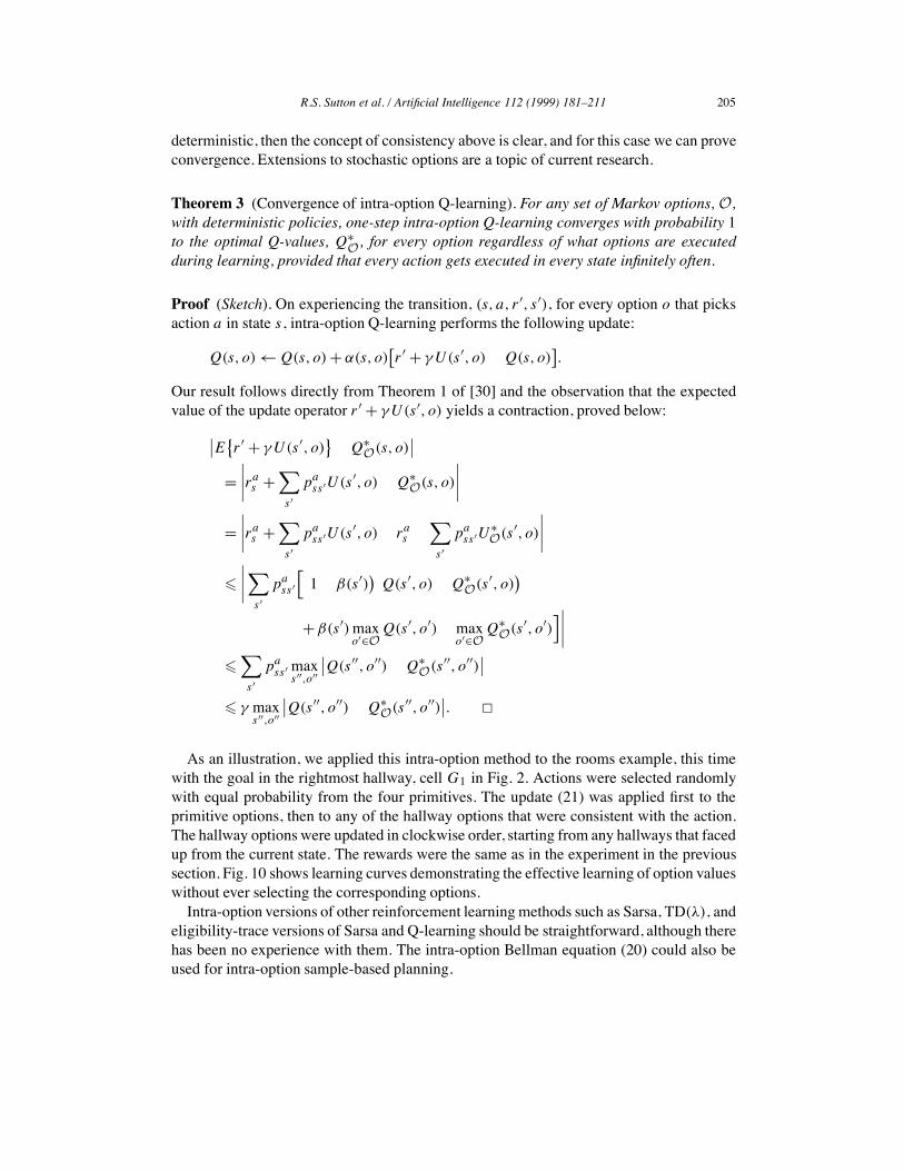
As an illustration, we applied this intra-option method to the rooms example, this timewith the goal in the rightmost hallway, cell G1 in Fig. 2. Actions were selected randomlywith equal probability from the four primitives. The update (21) was applied first to theprimitive options, then to any of the hallway options that were consistent with the action.The hallway options were updated in clockwise order, starting from any hallways that facedup from the current state. The rewards were the same as in the experiment in the previoussection. Fig. 10 shows learning curves demonstrating the effective learning of option valueswithout ever selecting the corresponding options.Intra-option versions of other reinforcement learning methods such as Sarsa, TD(*), and

eligibility-trace versions of Sarsa and Q-learning should be straightforward, although therehas been no experience with them. The intra-option Bellman equation (20) could also beused for intra-option sample-based planning.


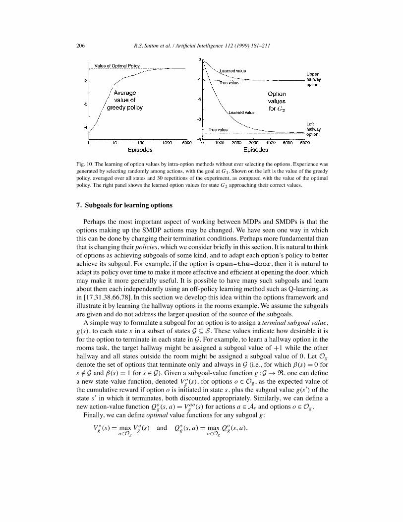
Fig. 10. The learning of option values by intra-option methods without ever selecting the options. Experience wasgenerated by selecting randomly among actions, with the goal at G1. Shown on the left is the value of the greedypolicy, averaged over all states and 30 repetitions of the experiment, as compared with the value of the optimalpolicy. The right panel shows the learned option values for state G2 approaching their correct values.

7. Subgoals for learning options

Perhaps the most important aspect of working between MDPs and SMDPs is that theoptions making up the SMDP actions may be changed. We have seen one way in whichthis can be done by changing their termination conditions. Perhaps more fundamental thanthat is changing their policies, which we consider briefly in this section. It is natural to thinkof options as achieving subgoals of some kind, and to adapt each option’s policy to betterachieve its subgoal. For example, if the option is open-the-door, then it is natural toadapt its policy over time to make it more effective and efficient at opening the door, whichmay make it more generally useful. It is possible to have many such subgoals and learnabout them each independently using an off-policy learning method such as Q-learning, asin [17,31,38,66,78]. In this section we develop this idea within the options framework andillustrate it by learning the hallway options in the rooms example. We assume the subgoalsare given and do not address the larger question of the source of the subgoals.A simple way to formulate a subgoal for an option is to assign a terminal subgoal value,

g(s), to each state s in a subset of states G & S . These values indicate how desirable it isfor the option to terminate in each state in G. For example, to learn a hallway option in therooms task, the target hallway might be assigned a subgoal value of +1 while the otherhallway and all states outside the room might be assigned a subgoal value of 0. Let Og

denote the set of options that terminate only and always in G (i.e., for which #(s) = 0 fors /" G and #(s) = 1 for s " G). Given a subgoal-value function g :G % R, one can definea new state-value function, denoted V o

g (s), for options o " Og , as the expected value ofthe cumulative reward if option o is initiated in state s, plus the subgoal value g(s#) of thestate s# in which it terminates, both discounted appropriately. Similarly, we can define anew action-value functionQo

g(s, a) = V aog (s) for actions a " As and options o " Og .

Finally, we can define optimal value functions for any subgoal g:

V !g (s) = max

o"Og

V og (s) and Q!

g(s, a) = maxo"Og

Qog(s, a).


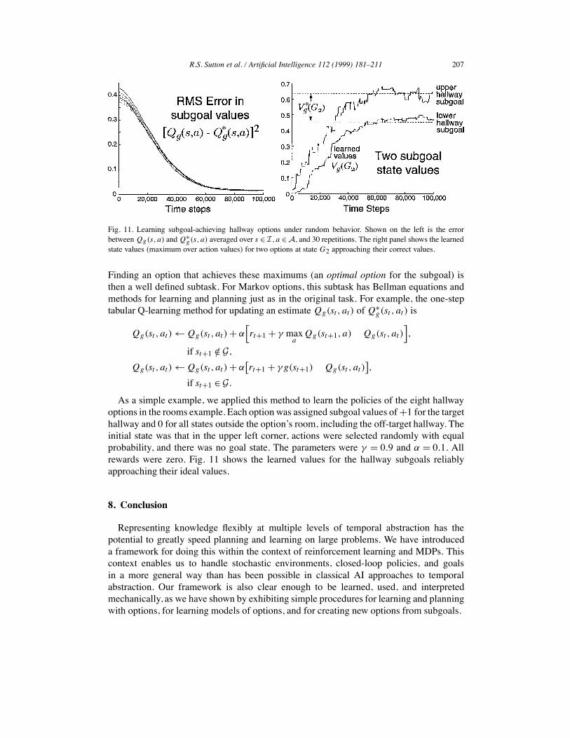
Fig. 11. Learning subgoal-achieving hallway options under random behavior. Shown on the left is the errorbetweenQg(s, a) andQ!

g(s, a) averaged over s " I , a " A, and 30 repetitions. The right panel shows the learnedstate values (maximum over action values) for two options at state G2 approaching their correct values.

Finding an option that achieves these maximums (an optimal option for the subgoal) isthen a well defined subtask. For Markov options, this subtask has Bellman equations andmethods for learning and planning just as in the original task. For example, the one-steptabular Q-learning method for updating an estimate Qg(st , at ) ofQ!

g(st , at ) is

Qg(st , at ) , Qg(st , at ) + '[rt+1 + " max

aQg(st+1, a) Qg(st , at )

],

if st+1 /" G,Qg(st , at ) , Qg(st , at ) + '[rt+1 + "g(st+1) Qg(st , at )

],

if st+1 " G.

As a simple example, we applied this method to learn the policies of the eight hallwayoptions in the rooms example. Each option was assigned subgoal values of+1 for the targethallway and 0 for all states outside the option’s room, including the off-target hallway. Theinitial state was that in the upper left corner, actions were selected randomly with equalprobability, and there was no goal state. The parameters were " = 0.9 and ' = 0.1. Allrewards were zero. Fig. 11 shows the learned values for the hallway subgoals reliablyapproaching their ideal values.

8. Conclusion

Representing knowledge flexibly at multiple levels of temporal abstraction has thepotential to greatly speed planning and learning on large problems. We have introduceda framework for doing this within the context of reinforcement learning and MDPs. Thiscontext enables us to handle stochastic environments, closed-loop policies, and goalsin a more general way than has been possible in classical AI approaches to temporalabstraction. Our framework is also clear enough to be learned, used, and interpretedmechanically, as we have shown by exhibiting simple procedures for learning and planningwith options, for learning models of options, and for creating new options from subgoals.


The foundation of the theory of options is provided by the existing theory of SMDPs andassociated learning methods. The fact that each set of options defines an SMDP providesa rich set of planning and learning methods, convergence theory, and an immediate,natural, and general way of analyzing mixtures of actions at different time scales. Thistheory offers a lot, but still the most interesting cases are beyond it because they involveinterrupting, constructing, or otherwise decomposing options into their constituent parts.It is the intermediate ground between MDPs and SMDPs that seems richest in possibilitiesfor new algorithms and results. In this paper we have broken this ground and touched onmany of the issues, but there is far more left to be done. Key issues such as transfer betweensubtasks, the source of subgoals, and integrationwith state abstraction remain incompletelyunderstood. The connection between options and SMDPs provides only a foundation foraddressing these and other issues.Finally, although this paper has emphasized temporally extended action, it is interesting

to note that there may be implications for temporally extended perception as well. It isnow common to recognize that action and perception are intimately linked. To see theobjects in a room is not so much to label or locate them as it is to know what opportunitiesthey afford for action: a door to open, a chair to sit on, a book to read, a person to talkto. If the temporally extended actions are modeled as options, then perhaps the models ofthe options correspond well to these perceptions. Consider a robot learning to recognizeits battery charger. The most useful concept for it is the set of states from which it cansuccessfully dock with the charger, and this is exactly what would be produced by themodel of a docking option. These kinds of action-oriented concepts are appealing becausethey can be tested and learned by the robot without external supervision, as we have shownin this paper.

Acknowledgement

The authors gratefully acknowledge the substantial help they have received from manycolleagues who have shared their related results and ideas with us over the long periodduring which this paper was in preparation, especially Amy McGovern, Ron Parr, TomDietterich, Andrew Fagg, B. Ravindran, Manfred Huber, and Andy Barto. We also thankLeo Zelevinsky, Csaba Szepesvári, Paul Cohen, Robbie Moll, Mance Harmon, SaschaEngelbrecht, and Ted Perkins. This work was supported by NSF grant ECS-9511805 andgrant AFOSR-F49620-96-1-0254,both to AndrewBarto and Richard Sutton. Doina Precupalso acknowledges the support of the Fulbright foundation. Satinder Singh was supportedby NSF grant IIS-9711753. An earlier version of this paper appeared as University ofMassachusetts Technical Report UM-CS-1998-074.

References

[1] E.G. Araujo, R.A. Grupen, Learning control composition in a complex environment, in: Proc. 4thInternational Conference on Simulation of Adaptive Behavior, 1996, pp. 333–342.

[2] M. Asada, S. Noda, S. Tawaratsumida, K. Hosada, Purposive behavior acquisition for a real robot by vision-based reinforcement learning, Machine Learning 23 (1996) 279–303.


[3] A.G. Barto, S.J. Bradtke, S.P. Singh, Learning to act using real-time dynamic programming, ArtificialIntelligence 72 (1995) 81–138.

[4] C. Boutilier, R.I. Brafman, C. Geib, Prioritized goal decomposition of Markov decision processes: Towarda synthesis of classical and decision theoretic planning, in: Proc. IJCAI-97, Nagoya, Japan, 1997, pp. 1162–1165.

[5] S.J. Bradtke, M.O. Duff, Reinforcement learning methods for continuous-time Markov decision problems,in: Advances in Neural Information Processing Systems 7, MIT Press, Cambridge, MA, 1995, pp. 393–400.

[6] R.I. Brafman, M. Tennenholtz, Modeling agents as qualitative decision makers, Artificial Intelligence 94 (1)(1997) 217–268.

[7] R.W. Brockett, Hybrid models for motion control systems, in: Essays in Control: Perspectives in the Theoryand its Applications, Birkhäuser, Boston, MA, 1993, pp. 29–53.

[8] L. Chrisman, Reasoning about probabilistic actions at multiple levels of granularity, in: Proc. AAAI SpringSymposium: Decision-Theoretic Planning, Stanford University, 1994.

[9] M. Colombetti, M. Dorigo, G. Borghi, Behavior analysis and training: A methodology for behaviorengineering, IEEE Trans. Systems Man Cybernet. Part B 26 (3) (1996) 365–380.

[10] R.H. Crites, A.G. Barto, Improving elevator performance using reinforcement learning, in: Advances inNeural Information Processing Systems 8, MIT Press, Cambridge, MA, 1996, pp. 1017–1023.

[11] P. Dayan, Improving generalization for temporal difference learning: The successor representation, NeuralComputation 5 (1993) 613–624.

[12] P. Dayan, G.E. Hinton, Feudal reinforcement learning, in: Advances in Neural Information ProcessingSystems 5, Morgan Kaufmann, San Mateo, CA, 1993, pp. 271–278.

[13] T. Dean, L.P. Kaelbling, J. Kirman, A. Nicholson, Planning under time constraints in stochastic domains,Artificial Intelligence 76 (1–2) (1995) 35–74.

[14] T. Dean, S.-H. Lin, Decomposition techniques for planning in stochastic domains, in: Proc. IJCAI-95,Montreal, Quebec, Morgan Kaufmann, San Mateo, CA, 1995, pp. 1121–1127. See also Technical ReportCS-95-10, Brown University, Department of Computer Science, 1995.

[15] G.F. DeJong, Learning to plan in continuous domains, Artificial Intelligence 65 (1994) 71–141.[16] T.G. Dietterich, The MAXQ method for hierarchical reinforcement learning, in: Machine Learning: Proc.

15th International Conference, Morgan Kaufmann, San Mateo, CA, 1998, pp. 118–126.[17] M. Dorigo, M. Colombetti, Robot shaping: Developing autonomous agents through learning, Artificial

Intelligence 71 (1994) 321–370.[18] G.L. Drescher, Made UpMinds: A Constructivist Approach to Artificial Intelligence, MIT Press, Cambridge,

MA, 1991.[19] C. Drummond, Composing functions to speed up reinforcement learning in a changing world, in: Proc. 10th

European Conference on Machine Learning, Springer, Berlin, 1998.[20] O. Etzioni, Why PRODIGY/EBL works, in: Proc. AAAI-90, Boston, MA, MIT Press, Cambridge, MA,

1990, pp. 916–922.[21] R.E. Fikes, P.E. Hart, N.J. Nilsson, Learning and executing generalized robot plans, Artificial Intelligence 3

(1972) 251–288.[22] H. Geffner, B. Bonet, High-level planning and control with incomplete information using POMDPs, in:

Proc. AIPS-98 Workshop on Integrating Planning, Scheduling and Execution in Dynamic and UncertainEnvironments, 1998.

[23] J. Gratch, G. DeJong, A statistical approach to adaptive problem solving, Artificial Intelligence 88 (1–2)(1996) 101–161.

[24] R. Greiner, I. Jurisica, A statistical approach to solving the EBL utility problem, in: Proc. AAAI-92, SanJose, CA, 1992, pp. 241–248.

[25] R.L. Grossman, A. Nerode, A.P. Ravn, H. Rischel, Hybrid Systems, Springer, New York, 1993.[26] M. Hauskrecht, N. Meuleau, C. Boutilier, L.P. Kaelbling, T. Dean, Hierarchical solution of Markov decision

processes using macro-actions, in: Uncertainty in Artificial Intelligence: Proc. 14th Conference, 1998,pp. 220–229.

[27] R. Howard, Dynamic Programming and Markov Processes, MIT Press, Cambridge, MA, 1960.[28] M. Huber, R.A. Grupen, A feedback control structure for on-line learning tasks, Robotics and Autonomous

Systems 22 (3–4) (1997) 303–315.[29] G.A. Iba, A heuristic approach to the discovery of macro-operators, Machine Learning 3 (1989) 285–317.


[30] T. Jaakkola, M.I. Jordan, S. Singh, On the convergence of stochastic iterative dynamic programmingalgorithms, Neural Computation 6 (6) (1994) 1185–1201.

[31] L.P. Kaelbling, Hierarchical learning in stochastic domains: Preliminary results, in: Proc. 10th InternationalConference on Machine Learning, Morgan Kaufmann, San Mateo, CA, 1993, pp. 167–173.

[32] Zs. Kalmár, Cs. Szepesvári, A. Lörincz, Module based reinforcement learning: Experiments with a realrobot, Machine Learning 31 (1998) 55–85 and Autonomous Robots 5 (1998) 273–295 (special joint issue).

[33] J. de Kleer, J.S. Brown, A qualitative physics based on confluences, Artificial Intelligence 24 (1–3) (1984)7–83.

[34] R.E. Korf, Learning to Solve Problems by Searching for Macro-Operators, Pitman Publishers, Boston, MA,1985.

[35] J.R. Koza, J.P. Rice, Automatic programming of robots using genetic programming, in: Proc. AAAI-92, SanJose, CA, 1992, pp. 194–201.

[36] B.J. Kuipers, Commonsense knowledge of space: Learning from experience, in: Proc. IJCAI-79, Tokyo,Japan, 1979, pp. 499–501.

[37] J.E. Laird, P.S. Rosenbloom, A. Newell, Chunking in SOAR: The anatomy of a general learning mechanism,Machine Learning 1 (1986) 11–46.

[38] L.-J. Lin, Reinforcement learning for robots using neural networks, Ph.D. Thesis, Carnegie MellonUniversity, Technical Report CMU-CS-93-103, 1993.

[39] P. Maes, R. Brooks, Learning to coordinate behaviors, in: Proc. AAAI-90, Boston, MA, 1990, pp. 796–802.[40] S. Mahadevan, J. Connell, Automatic programming of behavior-based robots using reinforcement learning,

Artificial Intelligence 55 (2–3) (1992) 311–365.[41] S. Mahadevan, N. Marchalleck, T. Das, A. Gosavi, Self-improving factory simulation using continuous-time

average-reward reinforcement learning, in: Proc. 14th International Conference on Machine Learning, 1997,pp. 202–210.

[42] P. Marbach, O. Mihatsch, M. Schulte, J.N. Tsitsiklis, Reinforcement learning for call admission control inrouting in integrated service networks, in: Advances in Neural Information Processing Systems 10, MorganKaufmann, San Mateo, CA, 1998, pp. 922–928.

[43] M.J. Mataric, Behavior-based control: Examples from navigation, learning, and group behavior, J. Experi-ment. Theoret. Artificial Intelligence 9 (2–3) (1997) 323–336.

[44] A. McGovern, R.S. Sutton, Macro-actions in reinforcement learning: An empirical analysis, TechnicalReport 98-70, University of Massachusetts, Department of Computer Science, 1998.

[45] N. Meuleau, M. Hauskrecht, K.-E. Kim, L. Peshkin, L.P. Kaelbling, T. Dean, C. Boutilier, Solving very largeweakly coupled Markov decision processes, in: Proc. AAAI-98, Madison, WI, 1998, pp. 165–172.

[46] S. Minton, Learning Search Control Knowledge: An Explanation-Based Approach, Kluwer Academic,Dordrecht, 1988.

[47] S. Minton, Quantitative results concerning the utilty of explanation-based learning, Artificial Intelligence 42(2–3) (1990) 363–391.

[48] A.W. Moore, The parti-game algorithm for variable resolution reinforcement learning in multidimensionalspaces, in: Advances in Neural Information Processing Systems 6, MIT Press, Cambridge, MA, 1994,pp. 711–718.

[49] A. Newell, H.A. Simon, Human Problem Solving, Prentice-Hall, Englewood Cliffs, NJ, 1972.[50] J. Nie, S. Haykin, A Q-learning based dynamic channel assignment technique for mobile communication

systems, IEEE Transactions on Vehicular Technology, to appear.[51] N. Nilsson, Teleo-reactive programs for agent control, J. Artificial Intelligence Res. 1 (1994) 139–158.[52] R. Parr, Hierarchical control and learning for Markov decision processes, Ph.D. Thesis, University of

California at Berkeley, 1998.[53] R. Parr, S. Russell, Reinforcement learning with hierarchies of machines, in: Advances in Neural Information

Processing Systems 10, MIT Press, Cambridge, MA, 1998, pp. 1043–1049.[54] D. Precup, R.S. Sutton, Multi-time models for reinforcement learning, in: Proc. ICML’97 Workshop on

Modeling in Reinforcement Learning, 1997.[55] D. Precup, R.S. Sutton, Multi-time models for temporally abstract planning, in: Advances in Neural

Information Processing Systems 10, MIT Press, Cambridge, MA, 1998, pp. 1050–1056.[56] D. Precup, R.S. Sutton, S.P. Singh, Planning with closed-loop macro actions, in: Working Notes 1997 AAAI

Fall Symposium on Model-directed Autonomous Systems, 1997, pp. 70–76.


[57] D. Precup, R.S. Sutton, S.P. Singh, Theoretical results on reinforcement learning with temporally abstractoptions, in: Proc. 10th European Conference on Machine Learning, Springer, Berlin, 1998.

[58] M.L. Puterman, Markov Decision Problems, Wiley, New York, 1994.[59] M. Ring, Incremental development of complex behaviors through automatic construction of sensory-motor

hierarchies, in: Proc. 8th International Conference on Machine Learning, Morgan Kaufmann, San Mateo,CA, 1991, pp. 343–347.

[60] E.D. Sacerdoti, Planning in a hierarchy of abstraction spaces, Artificial Intelligence 5 (1974) 115–135.[61] S. Sastry, Algorithms for design of hybrid systems, in: Proc. International Conference of Information

Sciences, 1997.[62] A.C.C. Say, S. Kuru, Qualitative system identification: Deriving structure from behavior, Artificial

Intelligence 83 (1) (1996) 75–141.[63] J. Schmidhuber, Neural sequence chunkers, Technische Universität München, TR FKI-148-91, 1991.[64] R. Simmons, S. Koenig, Probabilistic robot navigation in partially observable environments, in: Proc. IJCAI-

95, Montreal, Quebec, Morgan Kaufmann, San Mateo, CA, 1995, pp. 1080–1087.[65] S.P. Singh, Reinforcement learning with a hierarchy of abstract models, in: Proc. AAAI-92, San Jose, CA,

MIT/AAAI Press, Cambridge, MA, 1992, pp. 202–207.[66] S.P. Singh, Scaling reinforcement learning by learning variable temporal resolution models, in: Proc. 9th

International Conference on Machine Learning, Morgan Kaufmann, San Mateo, CA, 1992, pp. 406–415.[67] S.P. Singh, The efficient learning of multiple task sequences, in: Advances in Neural Information Processing

Systems 4, Morgan Kaufmann, San Mateo, CA, 1992, pp. 251–258.[68] S.P. Singh, Transfer of learning by composing solutions of elemental sequential tasks, Machine Learning 8

(3/4) (1992) 323–340.[69] S.P. Singh, A.G. Barto, R.A. Grupen, C.I. Connolly, Robust reinforcement learning in motion planning, in:

Advances in Neural Information Processing Systems 6, Morgan Kaufmann, San Mateo, CA, 1994, pp. 655–662.

[70] S.P. Singh, D. Bertsekas, Reinforcement learning for dynamic channel allocation in cellular telephonesystems, in: Advances in Neural Information Processing Systems 9, MIT Press, Cambridge, MA, 1997,pp. 974–980.

[71] R.S. Sutton, TD models: Modeling the world at a mixture of time scales, in: Proc. 12th InternationalConference on Machine Learning, Morgan Kaufmann, San Mateo, CA, 1995, pp. 531–539.

[72] R.S. Sutton, A.G. Barto, Reinforcement Learning: An Introduction, MIT Press, Cambridge, MA, 1998.[73] R.S. Sutton, B. Pinette, The learning of world models by connectionist networks, in: Proc. 7th Annual

Conference of the Cognitive Science Society, 1985, pp. 54–64.[74] R.S. Sutton, D. Precup, S. Singh, Intra-option learning about temporally abstract actions, in: Proc. 15th

International Conference on Machine Learning, Morgan Kaufmann, San Mateo, CA, 1998, pp. 556–564.[75] R.S. Sutton, S. Singh, D. Precup, B. Ravindran, Improved switching among temporally abstract actions, in:

Advances in Neural Information Processing Systems 11, MIT Press, Cambridge, MA, 1999, pp. 1066–1072.[76] M. Tambe, A. Newell, P. Rosenbloom, The problem of expensive chunks and its solution by restricting

expressiveness, Machine Learning 5 (3) (1990) 299–348.[77] G.J. Tesauro, Temporal difference learning and TD-Gammon, Comm. ACM 38 (1995) 58–68.[78] T. Thrun, A. Schwartz, Finding structure in reinforcement learning, in: Advances in Neural Information

Processing Systems 7, Morgan Kaufmann, San Mateo, CA, 1995, pp. 385–392.[79] M. Uchibe, M. Asada, K. Hosada, Behavior coordination for a mobile robot using modular reinforcement

learning, in: Proc. IEEE/RSJ International Conference on Intelligent Robots and Systems, 1996, pp. 1329–1336.

[80] C.J.C.H. Watkins, Learning with delayed rewards, Ph.D. Thesis, Cambridge University, 1989.[81] M. Wiering, J. Schmidhuber, HQ-learning, Adaptive Behavior 6 (2) (1997) 219–246.[82] L.E. Wixson, Scaling reinforcement learning techniques via modularity, in: Proc. 8th International

Conference on Machine Learning, Morgan Kaufmann, San Mateo, CA, 1991, pp. 368–372.

Documents

B etw een M D P s and sem i-M D P s: A fram ew ork …barto/courses/cs687/Sutton... · A fram ew ork for tem poralabstraction in reinforcem entlearning R ichard S .S utton a,!