Information Processing Letters 112 (2012) 411–417

Contents lists available at SciVerse ScienceDirect

Information Processing Letters

www.elsevier.com/locate/ipl

Bandwidth of convex bipartite graphs and related graphs ✩

Anish Man Singh Shrestha ∗, Satoshi Tayu, Shuichi Ueno

Department of Communications and Integrated Systems, Tokyo Institute of Technology, 2-12-1-S3-57 Ookayama, Meguro-ku, Tokyo, Japan

a r t i c l e i n f o a b s t r a c t

Article history:Received 5 October 2011Received in revised form 22 January 2012Accepted 7 February 2012Available online 28 February 2012Communicated by R. Uehara

Keywords:Approximation algorithmsBandwidth problem(Bi)convex bipartite graphs2-Directional orthogonal ray graphs

We show that the bandwidth problem is NP-complete for convex bipartite graphs. Weprovide an O (n)-time, 4-approximation algorithm and an O (n log2 n)-time, 2-approximationalgorithm to compute the bandwidth of convex bipartite graphs with n vertices. We alsoconsider 2-directional orthogonal ray graphs, a superclass of convex bipartite graphs, forwhich we provide an O (n2 log n)-time, 3-approximation algorithm, where n is the numberof vertices.

© 2012 Elsevier B.V. All rights reserved.

1. Introduction

A linear layout of an undirected graph G with vertexset V (G) and edge set E(G) is a bijection π : V (G) →{1,2, . . . , |V (G)|}. The bandwidth of (G,π ) is defined as

bπ (G) = max{∣∣π(u) − π(v)

∣∣ ∣∣ uv ∈ E(G)}.

The bandwidth of G , denoted b(G), is the smallest band-width over all linear layouts of G . A linear layout π ofG is said to be optimal if bπ (G) = b(G). The bandwidthproblem is to decide for a given graph G and k whetherb(G) � k. The bandwidth of a disconnected graph is themaximum bandwidth of its connected components. There-fore, we will consider only connected graphs.

Let G be a bipartite graph with bipartition (X, Y ). Anordering ≺ of X is said to fulfill the adjacency property iffor each y ∈ Y , the set of neighbors of y consists of ver-tices that are consecutive in ≺. G is said to be convex ifthere is an ordering of X that fulfills the adjacency prop-erty. G is said to be biconvex if there is an ordering ofX and an ordering of Y that fulfill the adjacency prop-

✩ A preliminary version of this article was presented at the 17th Inter-national Computing and Combinatorics Conference (COCOON), 2011.

* Corresponding author.E-mail address: anish@lab.ss.titech.ac.jp (A.M.S. Shrestha).

0020-0190/$ – see front matter © 2012 Elsevier B.V. All rights reserved.doi:10.1016/j.ipl.2012.02.012

erty. A bipartite graph which is also a permutation graphis called a bipartite permutation graph. For the definition ofpermutation graphs, we refer to [13]. A bipartite graph G issaid to be chordal if G contains no induced cycles of lengthgreater than 4. A tree is a chordal bipartite graph. A bipar-tite graph G with bipartition (X, Y ) is called a 2-directionalorthogonal ray graph if, in the xy-plane, there exist a fam-ily {Ra | a ∈ X} of horizontal rays (half-lines) extending inthe positive x-direction and a family {Rb | b ∈ Y } of ver-tical rays extending in the positive y-direction, such thattwo rays Ra and Rb intersect if and only if a and b areadjacent in G . The following relationship between theseclasses of graphs is known [3,12]: {Bipartite PermutationGraphs} ⊂ {Biconvex Bipartite Graphs} ⊂ {Convex Bipar-tite Graphs} ⊂ {2-Directional Orthogonal Ray Graphs} ⊂{Chordal Bipartite Graphs}.

Papadimitriou showed that the bandwidth problem isNP-complete for general graphs [11]. Monien showed thatit is NP-complete even for caterpillars of hair length atmost 3, which are very special trees [10]. This impliesthat it is also NP-complete for chordal bipartite graphs.On the other hand, Heggernes, Kratsch, and Meister re-cently showed that the bandwidth of bipartite permu-tation graphs can be computed in polynomial time [6].Uehara proposed a faster algorithm for the same prob-lem [15]. Polynomial-time algorithms are also known for

412 A.M.S. Shrestha et al. / Information Processing Letters 112 (2012) 411–417

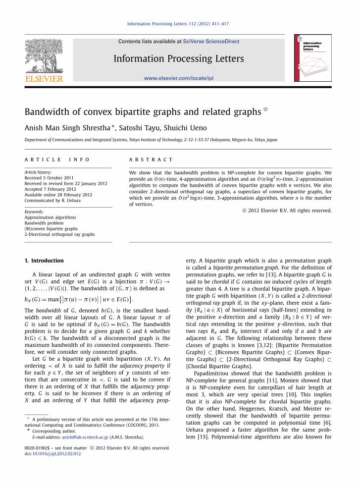
Fig. 1. Reduction from the multiprocessor scheduling problem to the bandwidth problem.

chain graphs [8], interval graphs [7], and caterpillars ofhair length at most 2 [1]. To the best of our knowledge,there are no prior results ascertaining the complexitiesof the bandwidth problem for 2-directional orthogonalray graphs, convex bipartite graphs, or biconvex bipartitegraphs. We show in Section 2 that the bandwidth problemis NP-complete even for convex trees and therefore also for2-directional orthogonal ray graphs. In Section 4, we showthat the problem can be solved in polynomial time for bi-convex trees.

Several results regarding approximation algorithms forcomputing bandwidth are known for general and specialgraph classes. Dubey, Feige, and Unger showed that evenfor generalized caterpillars (and therefore for chordal bi-partite graphs), it is NP-hard to approximate the band-width within any constant factor [5]. Polynomial-time,constant-factor approximation algorithms are known forfew special graph classes such as AT-free graphs and itssubclasses as shown by Kloks, Kratsch, and Müller [9]. Con-vex bipartite graphs or 2-directional orthogonal ray graphsare not contained in any of these classes. We provide inSection 3.1 an O (n)-time 4-approximation algorithm andan O (n log2 n)-time 2-approximation algorithm for convexbipartite graphs, and in Section 3.2 an O (n2 logn)-time 3-approximation algorithm for 2-directional orthogonal raygraphs, where n is the number of vertices of a graph.

2. NP-completeness result

A caterpillar is a tree in which all the vertices of degreegreater than one are contained in a single path called abody. An edge incident to a vertex of degree one is calleda hair. A generalized caterpillar is a tree obtained from acaterpillar by replacing each hair by a path. A path re-

placing a hair is also called a hair. Monien showed thefollowing [10]:

Theorem I. The bandwidth problem is NP-complete for gener-alized caterpillars of hair length at most 3. �

A convex tree is a convex bipartite graph that is a tree.We show the following.

Theorem 1. The bandwidth problem is NP-complete for convextrees.

Proof (Sketch). Except for a small modification in the con-struction of the convex tree, the proof is exactly the sameas that of Theorem I in [10] (where it appears as Theo-rem 1). Therefore we will provide only a proof sketch. As inthe proof of Theorem I, we reduce the multiple processorscheduling problem, which is known to be strongly NP-complete, to our problem. Given a set T = {t1, t2, . . . , tn}of tasks (ti being the execution time of task i), a dead-line D , and the size m of a set {1,2, . . . ,m} of processors,the multiple processor schedule problem asks whether thetasks in T can be scheduled on the m processors satisfy-ing the deadline D . Corresponding to an instance of thisproblem, a convex tree C is constructed as follows.

Each task ti is represented by a caterpillar Ti shownin Fig. 1(a). Each processor i is represented by a pathPi of length D − 1. Special components called “barrier”and “turning point” are constructed as shown in Figs. 1(b)and 1(c), respectively. C is constructed from these com-ponents as shown in Fig. 1(d), where p and � are integerswhose values we will fix later. Task caterpillars Ti and Ti+1are separated by a path Li of length �. Processor paths Piand Pi+1 are separated by a (p + 1)-barrier Bi . A turning

A.M.S. Shrestha et al. / Information Processing Letters 112 (2012) 411–417 413

point of height p + 2n + 1 separates the upper task portionand the lower processor portion. A (p + 2n + 1)-barrier B0is attached to the left of P1.

If we remove from C the degree-1 vertices of the turn-ing point, the remaining tree is a caterpillar. It is easyto see that a caterpillar is biconvex, and therefore bothpartitions of C have an ordering satisfying the adjacencyproperty. If we restore the degree-1 vertices, irrespectiveof their position in the ordering of their partition, they donot disturb the adjacency property of the ordering of theother partition. Thus C is a convex tree.

We will set the values of � and p such that � =2 × (m(D + 2) − 2) and p > 2n(D + 4). Then C can beconstructed in time polynomial in n, m, and D . It re-mains to be shown that the tasks in T can be scheduledon the m processors if and only if C has a bandwidth ofk = p + 1 + 2n. In fact, apart from the difference in thestructure of the turning point, this part of the proof is ex-actly the same as Lemmas 2 and 3 of [10]. Therefore, weshall only briefly describe the idea of the proof here. For adetailed treatment, we refer to Monien [10].

If there exists a scheduling of the tasks in T such thattasks ti1 , ti2 , . . . , ti j are assigned to processor i, then C hasbandwidth k and an optimal layout can be achieved by

(a) laying out the vertices of the body of Ti1 , Ti2 , . . . , Ti j

between barriers Bi−1 and Bi (between Bm−1 andturning point, for i = m) and

(b) laying out the vertices of B0 at the extreme left andthose of the turning point at the extreme right.

Conversely, if C has bandwidth k, then in any optimallayout of C ,

(a) the turning point must be laid out at one of the ex-treme ends, and barrier B0 must be laid out at theother,

(b) all the vertices of the body of each T j must be laidout between two barriers Bi and Bi+1 for some i (orBm−1 and the turning point for i = m − 1), and

(c) for each i, if between Bi and Bi+1 (or betweenBm−1 and turning point for i = m − 1), bodies ofTi1 , Ti2 , . . . , Ti j are laid out, then ti1 + ti2 + · · · +ti j < D .

This gives us a scheduling of the tasks in T . �Since the set of convex bipartite graphs is a proper sub-

set of the set of 2-directional orthogonal ray graphs, wehave the following corollary.

Corollary 1. The bandwidth problem is NP-complete for 2-directional orthogonal ray graphs.

3. Approximation algorithms

3.1. Approximation algorithms for convex bipartite graphs

We will present two algorithms that approximate thebandwidth of convex graphs with worst-case performanceratios of 2 and 4.

1 Compute m(i) for each vertex i ∈ Y . Add a dummy vertex|Y | + 1 to Y with m(|Y | + 1) = |X | + 1.

2 Let σ(1), . . . , σ (|Y + 1|) be the vertices of Y sorted in thenon-decreasing order of m(i) value, where σ is a permutationon {1, . . . , |Y | + 1}.

3 Initialize i ← 1, j ← 1, k ← 1.4 while ( j � |X |)5 if j < m(σ (i))6 π(x j) = k; j ← j + 1; k ← k + 1.

7 else if j = m(σ (i))8 π(σ (i)) = k; i ← i + 1; k ← k + 1.

9 return π

Fig. 2. Algorithm 1.

Let G be a convex bipartite graph with bipartition(X, Y ) and an ordering ≺ of X satisfying the adjacencyproperty with X = {x1, x2, . . . , x|X |} and x1 ≺ · · · ≺ x|X |.Assume Y = {1,2, . . . , |Y |}. Define mappings s : Y →{1,2, . . . ,n} and l : Y → {1,2, . . . ,n} such that for y ∈ Y ,xs(y) and xl(y) are, respectively, the smallest and largestvertices in ≺ adjacent to y. For each vertex y ∈ Y , letm(y) = �(s(y) + l(y))/2.

3.1.1. Algorithm 1Our first algorithm is described in Fig. 2. Algorithm 1

takes as input G along with the mappings s and l and out-puts a linear layout π of G . The idea of the algorithm isto lay out the vertices of X in the same order as they ap-pear in ≺ and insert the vertices of y between them, suchthat for each y ∈ Y , |NG(y)|/2� vertices of the set NG(y)

of its neighbors are onto its left and the remaining to itsright. Algorithm 1 starts by computing m(y) for each ver-tex of Y and sorting the vertices according to their m(i)values (lines 1 and 2). It incrementally assigns labels tothe vertices of X in the order in which they appear in ≺;stopping at each x j to check whether there is a vertex iny with m(y) value equal to j, in which case it assigns thecurrent label to y. The process is repeated until all verticeshave been labeled (lines 3 through 8).

We shall next analyze the performance of Algorithm 1.Consider a layout π output by Algorithm 1. The followinglemma is easy to see.

Lemma 1. Algorithm 1 preserves the ordering ≺ of X, i.e.,π(x1) < π(x2) < · · · < π(x|X |). �

For a vertex y ∈ Y , let G y be the subgraph of G inducedby the vertices in

V y = {v

∣∣ π(xs(y)) � π(v) � π(y)}

∪ {v

∣∣ π(y) � π(v) � π(xl(y))}.

The diameter of a graph is the least integer k such that ashortest path between any pair of vertices of the graph isat most k.

Lemma 2. For any y ∈ Y , the diameter of G y is at most 4.

Proof. We will prove this by showing that any vertex inV y is adjacent to a vertex in NG(y) ∪ {y}, where NG(y) is

414 A.M.S. Shrestha et al. / Information Processing Letters 112 (2012) 411–417

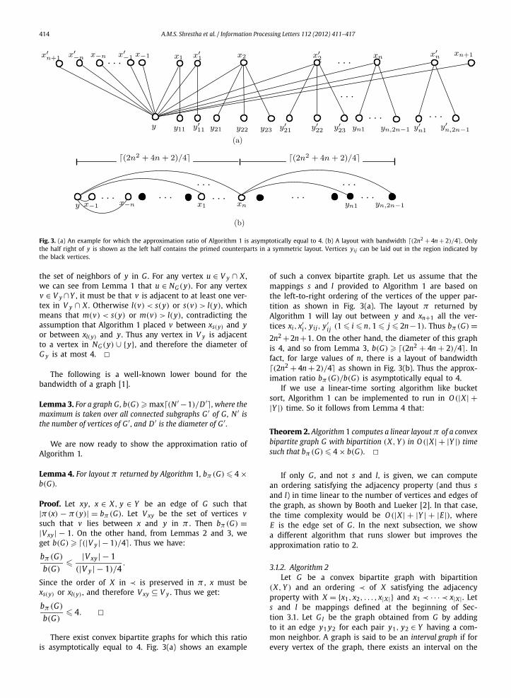
Fig. 3. (a) An example for which the approximation ratio of Algorithm 1 is asymptotically equal to 4. (b) A layout with bandwidth �(2n2 + 4n + 2)/4. Onlythe half right of y is shown as the left half contains the primed counterparts in a symmetric layout. Vertices yij can be laid out in the region indicated bythe black vertices.

the set of neighbors of y in G . For any vertex u ∈ V y ∩ X ,we can see from Lemma 1 that u ∈ NG(y). For any vertexv ∈ V y ∩Y , it must be that v is adjacent to at least one ver-tex in V y ∩ X . Otherwise l(v) < s(y) or s(v) > l(y), whichmeans that m(v) < s(y) or m(v) > l(y), contradicting theassumption that Algorithm 1 placed v between xs(y) and yor between xl(y) and y. Thus any vertex in V y is adjacentto a vertex in NG(y) ∪ {y}, and therefore the diameter ofG y is at most 4. �

The following is a well-known lower bound for thebandwidth of a graph [1].

Lemma 3. For a graph G, b(G) � max�(N ′ −1)/D ′, where themaximum is taken over all connected subgraphs G ′ of G, N ′ isthe number of vertices of G ′ , and D ′ is the diameter of G ′ .

We are now ready to show the approximation ratio ofAlgorithm 1.

Lemma 4. For layout π returned by Algorithm 1, bπ (G) � 4 ×b(G).

Proof. Let xy, x ∈ X, y ∈ Y be an edge of G such that|π(x) − π(y)| = bπ (G). Let V xy be the set of vertices vsuch that v lies between x and y in π . Then bπ (G) =|V xy| − 1. On the other hand, from Lemmas 2 and 3, weget b(G) � �(|V y | − 1)/4. Thus we have:

bπ (G)

b(G)� |V xy| − 1

(|V y| − 1)/4.

Since the order of X in ≺ is preserved in π , x must bexs(y) or xl(y) , and therefore V xy ⊆ V y . Thus we get:

bπ (G)

b(G)� 4. �

There exist convex bipartite graphs for which this ratiois asymptotically equal to 4. Fig. 3(a) shows an example

of such a convex bipartite graph. Let us assume that themappings s and l provided to Algorithm 1 are based onthe left-to-right ordering of the vertices of the upper par-tition as shown in Fig. 3(a). The layout π returned byAlgorithm 1 will lay out between y and xn+1 all the ver-tices xi, x′

i, yij, y′i j (1 � i � n,1 � j � 2n−1). Thus bπ (G) =

2n2 +2n+1. On the other hand, the diameter of this graphis 4, and so from Lemma 3, b(G) � �(2n2 + 4n + 2)/4. Infact, for large values of n, there is a layout of bandwidth�(2n2 + 4n + 2)/4 as shown in Fig. 3(b). Thus the approx-imation ratio bπ (G)/b(G) is asymptotically equal to 4.

If we use a linear-time sorting algorithm like bucketsort, Algorithm 1 can be implemented to run in O (|X | +|Y |) time. So it follows from Lemma 4 that:

Theorem 2. Algorithm 1 computes a linear layout π of a convexbipartite graph G with bipartition (X, Y ) in O (|X | + |Y |) timesuch that bπ (G) � 4 × b(G). �

If only G , and not s and l, is given, we can computean ordering satisfying the adjacency property (and thus sand l) in time linear to the number of vertices and edges ofthe graph, as shown by Booth and Lueker [2]. In that case,the time complexity would be O (|X | + |Y | + |E|), whereE is the edge set of G . In the next subsection, we showa different algorithm that runs slower but improves theapproximation ratio to 2.

3.1.2. Algorithm 2Let G be a convex bipartite graph with bipartition

(X, Y ) and an ordering ≺ of X satisfying the adjacencyproperty with X = {x1, x2, . . . , x|X |} and x1 ≺ · · · ≺ x|X | . Lets and l be mappings defined at the beginning of Sec-tion 3.1. Let G I be the graph obtained from G by addingto it an edge y1 y2 for each pair y1, y2 ∈ Y having a com-mon neighbor. A graph is said to be an interval graph if forevery vertex of the graph, there exists an interval on the

A.M.S. Shrestha et al. / Information Processing Letters 112 (2012) 411–417 415

real line, such that two intervals intersect if and only iftheir corresponding vertices are adjacent.

Lemma 5. G I is an interval graph.

Proof. We can see that G I is an interval graph by defininginterval [i, i] for each vertex xi ∈ X , and interval [s(y), l(y)]for each vertex y ∈ Y . �Lemma 6. b(G I )� 2b(G).

Proof. Let π be an optimal layout of G . Consider the samelayout of G I . For edge uv ∈ E(G I ) ∩ E(G),π(u) − π(v) �b(G). For edge uv ∈ E(G I ) \ E(G), there exists a commonneighbor of u and v in G , and therefore π(u) − π(v) �2b(G). Thus bπ (G I ) � 2b(G). Since b(G I ) � bπ (G I ), we getb(G I )� 2b(G). �

Sprague showed that given an interval model of an n-vertex interval graph G and a positive integer k, a layoutof bandwidth at most k, if one exists, can be constructedin O (n log n) time [14]. Thus by doing a binary search be-tween 1 and n, we can compute an optimal layout of G ,and therefore we have the following lemma.

Lemma 7. An optimal layout of an n-vertex interval graphcan be computed in O (n log2 n) time, if its interval model isgiven. �

Given a convex bipartite graph G and mappings s and l,Algorithm 2 simply constructs the interval model of G I

and applies the algorithm for interval graphs. The intervalmodel of G I can be constructed from s and l in time lin-ear to the number of vertices in G , and therefore we havefrom Lemmas 6 and 7 the following theorem:

Theorem 3. Algorithm 2 computes a linear layout π of a convexgraph G with n vertices in O (n log2 n) time such that bπ (G) �2 × b(G). �

For a path of length 3, whose bandwidth is 1, Algo-rithm 2 may return a layout of bandwidth 2. Therefore thisbound is tight.

3.2. Approximation algorithm for 2-directional orthogonal raygraphs

We will show a 3-approximation algorithm for 2-directional orthogonal ray graphs. Let G be a bipartitegraph with bipartition (X, Y ), and let (≺X ,≺Y ) be a pairof orderings of X and Y , respectively. Two edges x1 y1 andx2 y2 of G are said to cross in (≺X ,≺Y ) if x2 ≺X x1 andy1 ≺Y y2. If for every pair x1 y1 and x2 y2 that cross, x2 y1is also an edge of G , then (≺X ,≺Y ) is said to be a weakordering of G . If for every pair x1 y1 and x2 y2 of crossingedges, both x1 y2 and x2 y1 are edges of G , then (≺X ,≺Y )

is said to be a strong ordering of G .Spinrad, Brandstädt, and Stewart gave the following

characterization of bipartite permutation graphs [13].

Lemma 8. A graph G is a bipartite permutation graph if andonly if G has a strong ordering. �In an earlier work, we showed the following characteriza-tion of 2-directional orthogonal ray graphs [12].

Lemma 9. A graph G is a 2-directional orthogonal ray graph ifand only if G has a weak ordering. �

Given a 2-directional orthogonal ray graph G with bi-partition (X, Y ), edge set E , and a weak ordering (≺X ,≺Y )

of G , we can construct a graph G B P having vertex setV B P = X ∪ Y and edge set E B P = E ∪ E ′ , where E ′ is theset consisting of an edge x1 y2 for every pair of edges x1 y1and x2 y2 that cross in (≺X ,≺Y ).

Lemma 10. G B P is a bipartite permutation graph.

Proof. We will show that G B P is a bipartite permutationgraph by showing that (≺X ,≺Y ) is a strong ordering ofG B P .

Let e1 = x1 y1 and e2 = x2 y2 be two edges of G B P thatcross in (≺X ,≺Y ). We distinguish three cases: (Case 1)both e1, e2 ∈ E , (Case 2) one each of e1, e2 is in E ′ \ Eand E , and (Case 3) both e1, e2 ∈ E ′ \ E .

Case 1: Since (≺X ,≺Y ) is a weak ordering of G , x2 y1 ∈ E .By definition of E ′ , x1 y2 ∈ E ′ . Hence both x2 y1, x1 y2 ∈E B P .

Case 2: Without loss of generality, assume e1 ∈ E ′ \ E ande2 ∈ E . By definition of E ′ , e1 ∈ E ′ \ E implies that thereexist y′

1 ≺Y y1 and x′1 ≺X x1 such that x1 y′

1, x′1 y1 ∈ E

and they cross. Since x1 y′1 and x2 y2 also cross, x1 y2

must be in E ′ and therefore in E B P . To see that x2 y1 ∈E B P , we further distinguish three cases depending onthe order of x′

1 and x2 in ≺X .Case 2.1. x′

1 = x2: x2 y1 = x′1 y1 and hence x2 y1 ∈ E ⊆ E B P .

Case 2.2. x2 ≺X x′1: since x′

1 y1 and x2 y2 cross, x2 y1 ∈ E ⊆E B P .

Case 2.3. x′1 ≺X x2: since x1 y′

1 and x2 y2 cross, x2 y′1 ∈ E;

and x2 y′1 and x′

1 y1 cross, implying that x2 y1 ∈ E ′ ⊆E B P .

Case 3: By definition of E ′ , e1 ∈ E ′ \ E implies that thereexist y′

1 ≺Y y1 and x′1 ≺X x1 such that x1 y′

1, x′1 y1 ∈ E

and they cross. Again by definition of E ′ , e2 ∈ E ′ \ Eimplies that there exist y′

2 ≺Y y2 and x′2 ≺X x2 such

that x2 y′2, x′

2 y2 ∈ E and they cross. Since x1 y′1 and

x′2 y2 also cross, x1 y2 must be in E ′ and therefore in

E B P . To see that x2 y1 ∈ E B P , we further distinguishthree cases depending on the order of x′

1 and x2 in≺X .

Case 3.1. x′1 = x2: since x2 y1 = x′

1 y1, we have x2 y1 ∈ E ⊆E B P .

Case 3.2. x2 ≺X x′1: since x′

1 y1 ∈ E and x2 y2 ∈ E ′ \ E cross,we have x2 y1 ∈ E B P from Case 2.

Case 3.3. x′1 ≺X x2: we further distinguish three cases, de-

pending on the order of y′2 and y1 in ≺Y .

Case 3.3.1. y′2 = y1: since x2 y1 = x2 y′

2, we have x2 y1 ∈E ⊆ E B P .

416 A.M.S. Shrestha et al. / Information Processing Letters 112 (2012) 411–417

Case 3.3.2. y′2 ≺Y y1: since x2 y′

2 and x′1 y1 cross, x2 y1 ∈

E ′ ⊆ E B P .Case 3.3.3. y1 ≺Y y′

2: since x1 y1 ∈ E ′ \ E and x2, y′2 ∈ E

cross, we have x2 y1 ∈ E B P from Case 2.

In all the above subcases of Case 3, we have shown thatx1 y1 ∈ E B P , and hence both x2 y1, x1 y2 ∈ E B P .

Thus we have shown that for every e1 = x1 y1 and e2 =x2 y2 of G B P that cross in (≺X ,≺Y ), both x2 y1 and x1 y2are also edges of G B P ; and therefore from Lemma 8, G B P

is a bipartite permutation graph. �Lemma 11. b(G B P )� 3 × b(G).

Proof. Let π be an optimal layout of G . Consider thesame layout of G B P . For an edge xy of E(G B P ) ∩ E(G),|π(x) − π(y)| � b(G). For an edge xy of E(G B P ) \ E(G),there exist vertices x′ ∈ X and y′ ∈ Y such that yx′, x′ y, y′xare edges of G , and therefore |π(x) − π(y)| � 3 × b(G).Thus we have bπ (G B P ) � 3b(G). Since b(G B P ) � bπ (G B P ),we get b(G B P ) � 3 × b(G). �

We shall assume that along with a 2-directional orthog-onal ray graph G , a weak ordering (≺X ,≺Y ) is also pro-vided as input. If not, then such an ordering can be com-puted in O (n2) time, where n is the number of verticesof G [12]. We can construct G B P from G in O (n2) time.This can be done by first remembering for each x ∈ X , itssmallest neighbor yx in ≺Y and for each y ∈ Y , its smallestneighbor xy in ≺X , and then adding to G an edge xy foreach pair x, y for which yx ≺ y and xy ≺ x. Uehara showedthat an optimal layout of an n-vertex bipartite permutationgraph having bandwidth k can be computed in O (n2 log k)

time [15]. Then it follows from Lemma 11 that:

Theorem 4. There is an O (n2 log n)-time algorithm which com-putes a linear layout π of an n-vertex 2-directional orthogonalray graph G such that bπ (G) � 3 × b(G). �

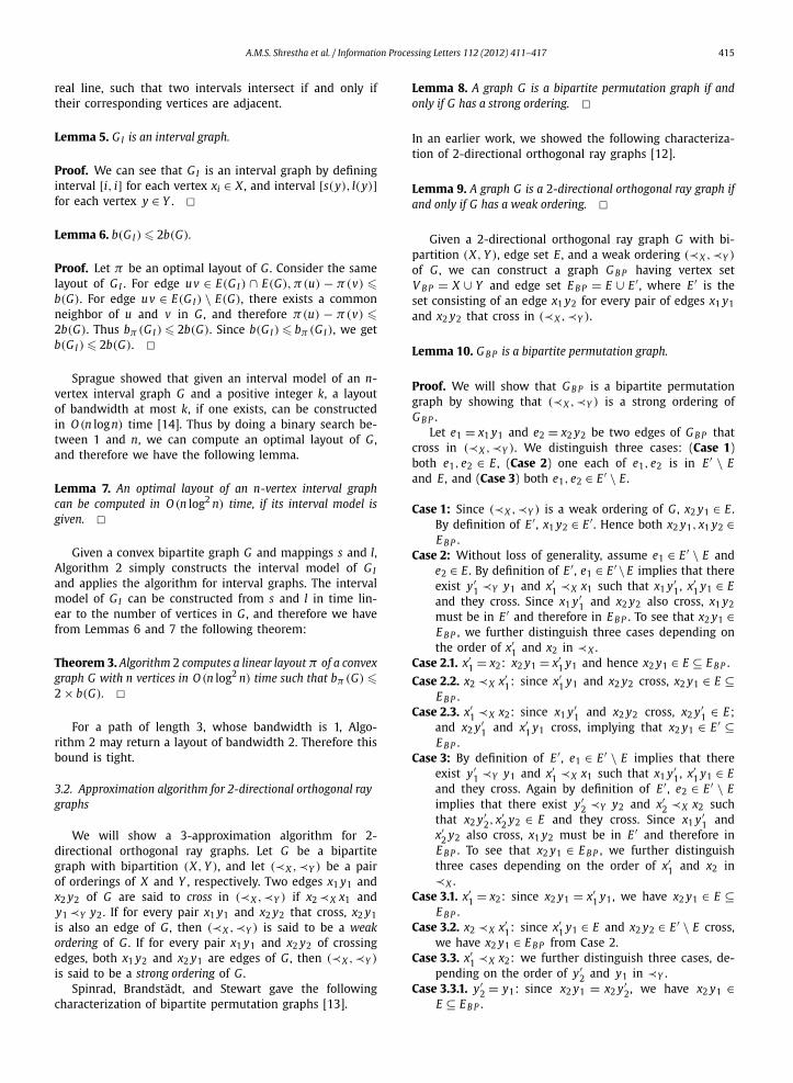
Although we do not yet know of an instance for whichthe ratio is 3, we show in Fig. 4(a), graph G for which thealgorithm returns a layout of bandwidth 2.5 times the op-timal. We can see that the ordering (≺X ,≺Y ) of G suchthat both ≺X and ≺Y are the top-to-bottom order of thevertices in Fig. 4(a) is a weak ordering. The correspond-ing bipartite permutation graph G B P is shown in Fig. 4(b).The bandwidth of G is 2. G B P contains a complete bipar-tite graph K4,3 induced by the round vertices. Since it isknown [4] that b(Km,n) = (m − 1)/2� + n for m � n > 0,we have b(G B P ) � 4. It can be quickly checked that ifb(G B P ) = 4, then in any optimal layout, the black verticesmust be laid out as one contiguous block with two of theremaining round vertices on either side of the block. Thesquare vertex, which is adjacent to three round vertices,cannot be placed anywhere without increasing the band-width of the layout. Thus b(G) > 4. On the other hand,a layout of bandwidth 5 can be easily obtained.

Fig. 4. 2-Directional orthogonal ray graph G for which the approximationratio is 2.5.

4. Bandwidth of biconvex graphs

Although we do not yet know the complexity of band-width problem for biconvex graphs, we have a partial re-sult. We show that it can be solved in polynomial time forbiconvex trees. The 2-claw is a graph obtained from thecomplete bipartite graph K1,3 by replacing each edge by apath of length 2. The following lemma can be quickly ver-ified.

Lemma 12. The 2-claw is not a biconvex tree. �Biconvex trees can be characterized as follows:

Lemma 13. A tree T is biconvex if and only if T is a caterpillar.

Proof. The sufficiency is easy. To prove the necessity, sup-pose T is a biconvex tree. Let P be a longest path in T . Ifthe length of P is less than five, T is trivially a caterpil-lar, and so we assume that it is greater than five. Supposethere exists a vertex not in P having degree greater than 1.This implies that T contains the 2-claw as a subtree, con-tradicting the assumption that T is biconvex graph. There-fore T is a caterpillar. �

Since a caterpillar is an interval graph, bandwidth ofbiconvex trees can be computed in polynomial time.

5. Concluding remarks

We note that the complexity of bandwidth problemfor biconvex graphs remains an interesting open ques-tion. Also, the analysis we presented for our approximationalgorithm for 2-directional orthogonal ray graphs is nottight, and closing the gap is another open question.

References

[1] S.F. Assmann, G.W. Peck, M.M. Sysło, J. Zak, The bandwidth of cater-pillars with hairs of length 1 and 2, SIAM J. Algebraic Discrete Meth-ods 2 (4) (1981) 387–393.

[2] K.S. Booth, G.S. Lueker, Testing for the consecutive ones property, in-terval graphs, and graph planarity using PQ-tree algorithms, J. Com-put. Syst. Sci. 13 (3) (1976) 335–379.

[3] A. Brandstädt, V.B. Le, J.P. Spinrad, Graph Classes: A Survey, Societyfor Industrial and Applied Mathematics, 1999.

[4] V. Chvátal, A remark on a problem of Harary, Czechoslovak Math.J. 20 (1) (1970) 109–111.

[5] C. Dubey, U. Feige, W. Unger, Hardness results for approximating thebandwidth, J. Comput. Syst. Sci. 77 (2011) 62–90.

A.M.S. Shrestha et al. / Information Processing Letters 112 (2012) 411–417 417

[6] P. Heggernes, D. Kratsch, D. Meister, Bandwidth of bipartite permu-tation graphs in polynomial time, J. Discrete Algorithms 7 (4) (2009)533–544.

[7] D. Kleitman, R. Vohra, Computing the bandwidth of interval graphs,SIAM J. Discrete Math. 3 (1990) 373–375.

[8] T. Kloks, D. Kratsch, H. Müller, Bandwidth of chain graphs, Inf. Pro-cess. Lett. 68 (6) (1998) 313–315.

[9] T. Kloks, D. Kratsch, H. Müller, Approximating the bandwidth for as-teroidal triple-free graphs, J. Algorithms 32 (1999) 41–57.

[10] B. Monien, The bandwidth minimization problem for caterpillarswith hair length 3 is NP-complete, SIAM J. Algebraic Discrete Meth-ods 7 (4) (1986) 505–512.

[11] C. Papadimitriou, The NP-completeness of the bandwidth minimiza-tion problem, Computing 16 (1976) 263–270.

[12] A.M.S. Shrestha, S. Tayu, S. Ueno, On orthogonal ray graphs, DiscreteAppl. Math. 158 (2010) 1650–1659.

[13] J. Spinrad, A. Brandstädt, L. Stewart, Bipartite permutation graphs,Discrete Appl. Math. 18 (3) (1987) 279–292.

[14] A.P. Sprague, An O (n logn) algorithm for bandwidth of intervalgraphs, SIAM J. Discrete Math. 7 (2) (1994) 213–220.

[15] R. Uehara, Bandwidth of bipartite permutation graphs, in: 19thAnnual International Symposium on Algorithms and Computation,in: Lecture Notes in Computer Science, vol. 5369, 2008, pp. 824–835.