Bank Diversification, Market

Structure and Bank Risk Taking:

Theory and Evidence from U.S.

Commercial Banks

Martin Goetz ∗

January 17, 2012

Abstract

This paper studies how a bank’s diversification affects its own risk taking

behavior and the risk taking of competing, nondiversified banks. By combin-

ing theories of bank organization, market structure and risk taking, I show

that greater geographic diversification of banks changes a bank’s lending be-

havior and market interest rates, which also has ramifications for nondiversi-

fied competitors due to interactions in the banking market. Empirical results

obtained from the U.S. commercial banking sector support this relationship

as they indicate that a bank’s risk taking is lower when its competitors have

a more diversified branch network. By utilizing the state-specific timing of a

removal of intrastate branching restrictions in two identification strategies, I

further pin down a causal relationship between the diversification of competi-

tors and a bank’s risk taking behavior. These findings indicate that a bank’s

diversification also impacts the risk taking of competitors, even if these banks

are not diversifying their activities.

JEL Classification: G21, G32, L22

Keywords: Risk Taking, Organization, Commercial Banks, Diversification,

Competition

∗Federal Reserve Bank of Boston, 600 Atlantic Avenue, Boston MA 02210. Email: Mar-tin.Goetz@bos.frb.org. Tel.: (617) 973 3018Financial support from the Networks Financial Institute (Indiana State University) is greatly ap-preciated. I am very thankful to Ross Levine, Nicola Cetorelli, Marcia Millon Cornett, RubenDurante, Tatiana Farina, Andy Foster, Juan Carlos Gozzi, Luc Laeven, Alex Levkov, Jose Liberti,Blaise Melly, Donald Morgan, and David VanHoose for helpful comments and discussions. I alsothank seminar participants at , the Bank for International Settlements, Banque de France, Bent-ley College, Board of Governors, Brown University, European Business School, European CentralBank, Federal Reserve Bank of Boston, and Tilburg University for many comments and sugges-tions. The views expressed in this paper are solely those of the author and do not necessarilyreflect official positions of the Federal Reserve Bank of Boston or the Federal Reserve System.

1 Introduction

In this paper, I address one of the most basic questions in banking: are banks

with lending activities in several banking markets safer than banks that focus their

operations on a single market? Expanding lending operations into more markets

allows banks to diversify risk across regions, and if loan returns across regions are

not perfectly correlated, geographically diversified banks are safer because they are

less exposed to shocks that hit individual areas (Diamond (1984); Demsetz and

Strahan (1997); Morgan et al. (2004)). Banks’ risk taking is also related to market

structure, and risk taking could change because diversification across markets affects

competition in banking markets. Competition for borrowers might intensify as banks

expand their operations, which decreases a bank’s rents, erodes its charter value,

and therefore provides incentives for banks to take on more risk (Keeley (1990)).

However, greater competition might also lead to lower loan rates, which reduces the

extent of borrowers’ risk shifting incentives and thus reduces a bank’s exposure to

risk of failure (Boyd and de Nicolo (2005)).

While many researchers examine the connection between bank diversification

and risk taking, none consider how the interactions between banks that diversify and

banks that focus their operations affect the fragility of these different banks. This

omission turns out to be of first-order importance both conceptually and empirically.

This paper provides more information on the relationship between bank diversifica-

tion and risk taking by (1) explicitly modeling the interactions between banks that

diversify geographically and those that focus their operations, and (2) providing

empirical evidence from the U.S. banking sector, consistent with the model.

The model incorporates theories of market structure and risk taking (Boyd and

de Nicolo (2005); Martinez-Miera and Repullo (2010)) and theories of bank struc-

ture and behavior (Stein (2002); Acharya et al. (2011)) to study the effect of banks’

diversification on risk taking. By highlighting the relationship between bank man-

1

ager and loan officers within banks, I show that loan officers have an incentive to

shift lending towards certain borrower types when banks expand their branch net-

work. Because of competition for borrowers, a shift in lending affects market loan

interest rates and changes a bank’s loan portfolio risk. This determines a bank’s

risk taking behavior. Furthermore, the shift in lending also impacts the behavior of

competitors, which affects their exposure to risk of failure. Hence, the model shows

that a bank’s geographic diversification not only affects its own risk taking, but also

shapes the risk taking behavior of other banks due to competition in the banking

market. This model adds to the debate on diversification, market structure and risk

taking by showing an additional channel that affects banks’ risk taking.

I use information from the U.S. commercial banking sector to empirically exam-

ine the relationship between a bank’s geographical diversification, the diversity of

its competitors and the risk taking behavior of these different banks. By examining

banks’ level of geographic diversification across counties within a state, I find that

a bank’s risk taking is lower when its competitors have a more diversified branch

network across counties. This finding is also robust to alternative measures of risk

taking and diversification. While these results are consistent with the theoretical

framework they do, however, not reflect a causal relationship since unobservable

factors, such as bank efficiency, might exert an influence on a bank’s risk taking

behavior.

To estimate the causal impact of a bank’s diversification on competing banks’

risk taking, I employ two empirical strategies based on (1) the timing of intrastate

branching deregulation and (2) a gravity model, which explains a bank’s expansion

behavior within a state (Goetz et al. (2011)). Because banks were not allowed to

expand their branch network freely within state borders before the removal of these

branching restrictions, I can identify the exogenous component of banks’ expansion

activity, as each identification strategy utilizes the state specific timing of a removal

2

of intrastate branching restrictions to determine an exogenous change in banks’

diversification. This allows me to pin down the causal effect of a bank’s degree of

diversification on its risk taking behavior and the risk taking behavior of competitors.

The first empirical strategy uses heterogeneity in the timing of intrastate branch-

ing deregulation across states as an instrument for the average bank’s diversification

within state borders. I find robust evidence that the failure risk of a bank decreases

when competitors diversify across banking markets. Moreover, this effect is also eco-

nomically significant: a bank’s annual risk of failure decreases by approximately 20

% if competitors increase their geographic diversification by one standard deviation.

To further strengthen my results, I combine the timing of intrastate branching

deregulation with a gravity model of bank expansion within a state in the second

identification strategy to construct an instrumental variable at the bank level.1 By

imbedding the timing of intrastate branching deregulation within a gravity model, I

determine for each bank and year its projected level of diversity using this gravity-

deregulation model (Goetz et al. (2011)). In a second step, I then use this instru-

mental variable to estimate the effect of diversification on risk taking.

Because the gravity-deregulation model explains expansion at the bank level

for each year, I can (1) account for a bank’s endogenous decision to expand, and

(2) capture unobservable state specific time-varying influences by including a set

of state specific time fixed effects in the regression model. Using this identification

strategy, I test whether the impact of a bank’s expansion on its own risk of fail-

ure is different than the impact on competitors’ risk taking, as highlighted by the

model. Results from the gravity-deregulation model confirm the earlier findings and

support the theorized link between a bank’s diversification, its competitors’ level of

diversification and their risk taking behavior.

The main contribution of this paper is the theoretical and empirical identification

1I follow the methodology from Frankel and Romer (1999) who analyze whether and howinternational trade flows affect economic growth.

3

of a direct effect of a bank’s diversification on its own risk taking and the risk taking

behavior of competitors. This adds to the debate on bank risk taking, market struc-

ture and bank organization, since my empirical results do not reject earlier theories

and findings, but rather complement existing studies by identifying a further chan-

nel that affects bank risk taking. Although the theoretical framework incorporates

findings on the relationship between bank organization and individual loan officers’

behavior (Liberti and Mian (2009), Hertzberg et al. (2010)), I do not empirically

assess the impact of a bank’s organizational structure on individual loan officers’ risk

taking behavior within a bank. Moreover, I focus on the firm-wide effects of changes

in a bank’s diversification on its risk taking and the risk taking of competitors in this

paper. Furthermore, this paper is also related to studies of market structure and

bank risk taking, based on regression results from cross-country analysis (de Nicolo

(2000), Boyd et al. (2007)), and evidence from the Great Depression (Calomiris and

Mason (2000), Mitchener (2005)).

The remainder of this paper is organized as follows: in Section 2, I provide a

theoretical framework studying the relationship between a bank’s level of diversi-

fication, the degree of competitors’ diversification and their risk taking behavior.

Following this, I present OLS regression results using information from U.S. com-

mercial banks in Section 3. Empirical results on the causal relationship between

diversification and risk taking is presented in Section 4. Section 5 concludes the

paper.

2 Theoretical Framework

I build on Stein (2002) to show (1) how a bank’s level of geographic diversification

affects its risk taking and (2) the risk taking of competing banks. Stein (2002)

and Berger et al. (2005) show that banks’ organizational structure (decentraliza-

4

tion versus hierarchy) determines their ability to produce and process information

about borrowers. This has effects on banks’ lending behavior as banks with a flatter

organizational structure, and thus less diversification, are better at lending to soft

information borrowers. The theoretical model is also related to theories highlight-

ing the relationship between bank competition and lending relationships (Petersen

and Rajan (1995), Dell’Ariccia and Marquez (2004)), and theories regarding the

structure of banks and their behavior (Dell’Ariccia and Marquez (2010), Boot and

Schmeits (2000)).

2.1 Model

Borrowers There is a mass of entrepreneurs with access to a risky technology

which yields R with probability p(e). By increasing effort e at cost 12e2, an en-

trepreneur’s likelihood of success p(e) increases. Moreover, an entrepreneur’s like-

lihood of success is independent of other entrepreneurs’ success probabilities. For

any given level of effort, the success probability is less than one, and concave in

effort with p(0) = 0.5. Effort is unobservable and not verifiable to third parties. En-

trepreneurs seek financing from banks, but differ in the level of collateral they can

pledge when taking out a loan; some borrowers can pledge collateral λ when taking

out a loan. Since collateral λ is observable and verfiable, borrowers with collateral

are called “hard information” borrowers. Similarly, borrowers without collateral are

referred to as “soft information” borrowers. In case a hard information borrower is

not successful (with probability 1− p), the bank receives that borrower’s collateral

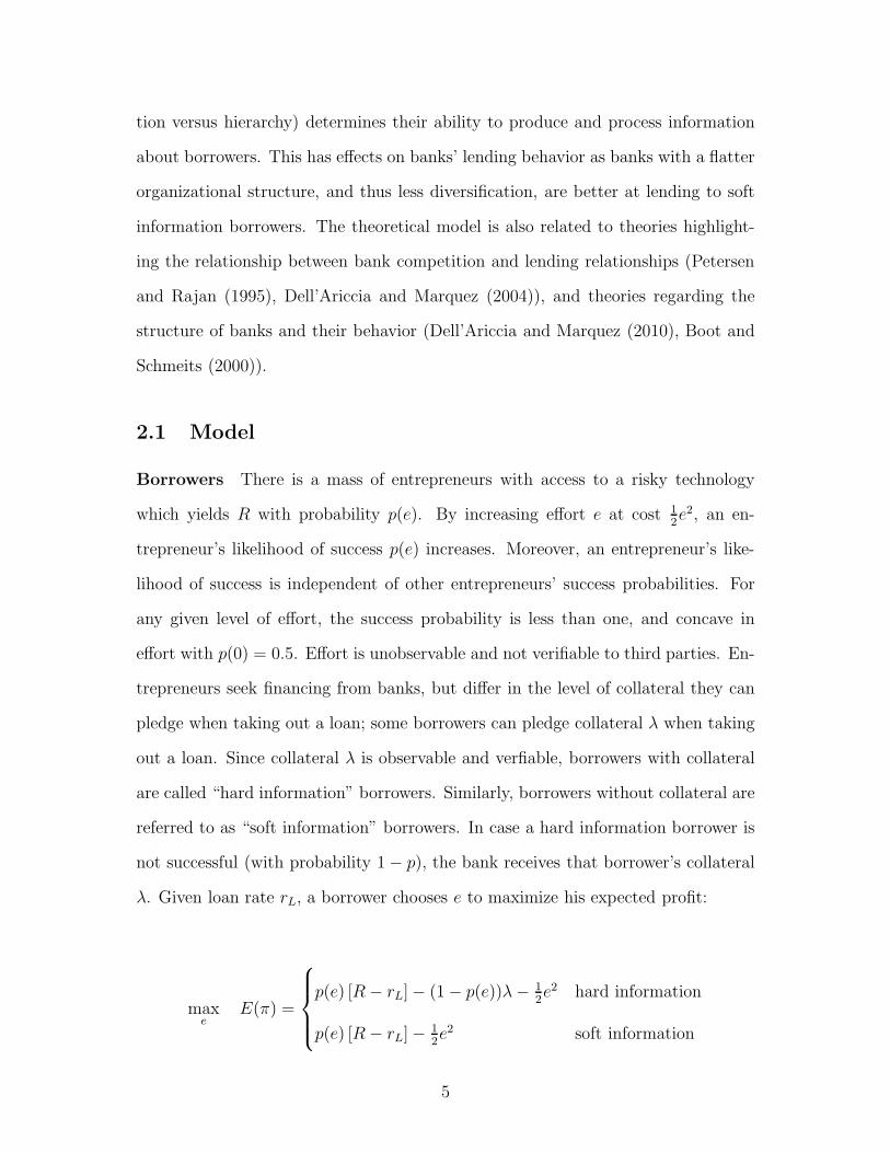
λ. Given loan rate rL, a borrower chooses e to maximize his expected profit:

maxe

E(π) =

p(e) [R− rL]− (1− p(e))λ− 12e2 hard information

p(e) [R− rL]−12e2 soft information

5

Similar to Boyd and de Nicolo (2005), it can be shown that borrowers in this

model shift risk towards banks when banks increase the loan rate. Entrepreneurs

also differ in their unobservable outside option, denoted π̄, which determines whether

an entrepreneur will borrow or not. There is a continuum of borrowers in the

market, defined by a continuous distribution of outside options with support R+.

The measure of borrowers with an outside option of at most π̄ is denoted as F (π̄).

For simplicity hard and soft information borrowers have different outside options,

e.g. π̄S = π̄H +λ.2 An entrepreneur takes out a loan at rate rL if his expected profit

is greater or equal than his outside option. The measure of borrowers at loan rate

rL is denoted F (π(rL)), which yields loan demand D (Martinez-Miera and Repullo

(2010)):

D(rL) = F (π(rL))

Loan demand is decreasing in the loan interest rate rL, D′(rL) = F ′(π(rL))π

′(rL) <

0. Inverse loan demand is denoted by rL(D) with r′L(D) < 0.

Banks Banks differ in their organizational structure which is characterized by a

bank’s number of branches. The number of branches also determines the number of

distinct banking markets a bank is active in, and thus reflects its level of geographic

diversification. Each branch consists of a loan officer that decides on lending, and

branches of the same bank do not compete for borrowers within the same market.

Further, each bank also consists of a CEO (see below).

Loan officers make lending decision in bank branches. Their lending decision is

shaped by (a) competition in the market for borrowers (horizontal competition), and

(b) the possibility to become the next CEO (Acharya et al. (2011)) (vertical com-

petition). Because borrower types are observable, loan officers face a loan demand

DS/DH for soft/hard information borrowers. Moreover, loan officers in a market

2This ensures that the measure of borrowers demanding loans at a given level of outside optionis not affected by the availability of collateral.

6

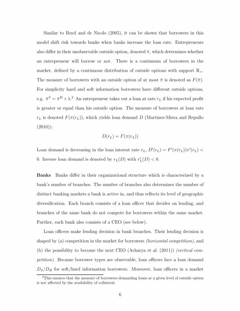
compete for borrowers a la Cournot and each loan officer has one unit of funding

available, which he allocates between soft and hard information borrowers. Suppose

the total supply of credit to hard information borrowers in a market is denoted by

A.3 Expected profits from lending to hard/soft information borrowers are given as

µH/µS:

µH = pH(A)(1 + rH(A)) + (1− pH(A))λ

µS = pS(A)(1 + rS(A))

Loan officers choose a loan portfolio β (= share of loans to hard information

borrowers) to maximize their expected profit.

A bank’s CEO receives a fraction γ of every branch’s expected profit, and his

only role is evaluating every loan officer to determine his successor. In particular, he

observes each loan officers profit at cost c - where c is decreasing in a loan officer’s

choice of β4 - and chooses the loan officer with the highest profit net of the evaluation

cost to be the next CEO.5

Horizontal Competition (within markets) Each loan officer in a market chooses

to lend a fraction of its funding to hard information borrowers in that market.

For simplicity, suppose there are two branches of competing banks in that mar-

ket. Let the fraction of lending by loan officer a be denoted by α, and the fraction

of loan officer b by β. Total lending to hard information borrowers in this mar-

ket is then A = α + β. Expected profits for loan officer b is therefore given as:

E(π) = [βµH(A) + (1− β)µS(A)]× (1− γ).

3Because the total amount of credit within a market is limited by the number of branches,expected profits from lending to soft information borrowers are also determined by A.

4The rationale is that it is less costly for the CEO to evaluate a loan portfolio of hard informationborrowers.

5A loan officer’s choice of β also affects his chance of becoming the next CEO. If a bank hasonly one branch, the loan officer will become the next CEO with certainty. However, loan officersin banks with more than one branch compete with each other to become the next CEO.

7

Vertical Competition (within banks) Suppose a bank has two branches, and

let loan officers in the branches of this bank be labeled i and j. Each loan officer

chooses a fraction βi, βj of lending to hard information borrowers in his respective

banking market. Loan officer i will become the next CEO if his profit net of evalua-

tion cost (πi−ci) are larger than j’s net profit (πj−cj). Because evaluation costs are

decreasing in the loan officer’s share of hard information borrowers, the probability

of becoming the next CEO for loan officer i (pri) increases in βi (see appendix for

details).6

2.2 Equilibrium and Comparative Statics

2.2.1 Equilibrium

In equilibrium, banks discriminate between hard and soft information borrowers, and

offer a separate interest rate for each borrower type. Denote the CEO’s equilibrium

net profit from each branch as Π, and suppose there are two branches (i, j). Loan

officer i then chooses βi to maximize:

maxβi

(1− γ) E (πi(βi)) + pri(βi, βj)× 2γ

1 + ρ

[

Π̄]

(1)

Since loan demand is increasing in interest rates, there is an optimal allocation

of lending between soft and hard information borrowers.

2.2.2 Comparative Statics

Competition within a market For simplicity, I focus on the case of two banks

and two branches. Let the choice of loan officers’ share of hard information loans

in different banks be denoted by α and β, and the share of loan officers of the same

bank be denoted by βi and βj. Because loan officers within a market compete for

6This is similar to a result from first priced sealed bid auctions.

8

borrowers a la Cournot, loan officers have an incentive to differentiate themselves

from each other:

Proposition 1 (Differentiation) A loan officer’s share of hard information bor-

rowers is negatively related to its competitor’s choice of hard information borrowers.

Suppose a competing branch increases lending to hard information borrowers.

Because total credit supply in a banking market is limited and loan officers compete

for borrowers a la Cournot, interest rates for hard information borrowers decrease,

while interest rates for soft information borrowers increase. This makes lending to

soft information borrowers more profitable, which induces a loan officer to increase

lending to soft information borrowers.

Competition within banks It can be shown that loan officers in banks with

more branches will choose a loan portfolio with a larger share of hard information

borrowers.

Proposition 2 (Effect of hierarchy on β) A loan officer in a bank with more

branches chooses a larger β than a loan officer in a bank with less branches.

This result is similar to Stein (2002). While Stein (2002) shows that internal

capital markets in more hierarchical banks lead to a larger share of hard information

borrowers, the mechanism here is the tournament between loan officers for the bank’s

CEO position (Acharya et al. (2011)).

2.3 Risk

2.3.1 Loan Portfolio Risk

In equilibrium, branches lend to a continuum of soft and hard information borrow-

ers. Repayment by each borrower is stochastic and independent within and across

9

borrower types. Further, due to symmetry, each borrower type chooses the same

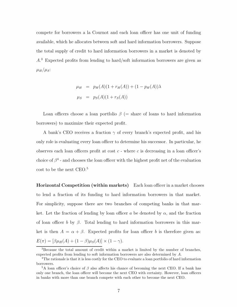
level of effort and exhibits the same repayment probability. Suppose, a bank’s loan

portfolio consists of infinitely granular soft and hard information borrowers and is

given byX . Because profit from lending to a borrower type is binomially distributed,

X can be approximated by a normal distribution with mean µB and variance σ2B,

where

µB = βµH + (1− β)µS

σ2B = β2σ2

H + (1− β)2σ2S,

σ2H and σ2

S is the variance of hard and soft information borrowers, respectively.

2.3.2 Risk Taking

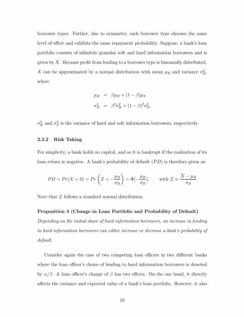
For simplicity, a bank holds no capital, and so it is bankrupt if the realization of its

loan return is negative. A bank’s probability of default (PD) is therefore given as:

PD = Pr(X < 0) = Pr

(

Z < −µB

σB

)

= Φ(−µB

σB

), with Z ≡X − µB

σB

Note that Z follows a standard normal distribution.

Proposition 3 (Change in Loan Portfolio and Probability of Default)

Depending on the initial share of hard information borrowers, an increase in lending

to hard information borrowers can either increase or decrease a bank’s probability of

default.

Consider again the case of two competing loan officers in two different banks

where the loan officer’s choice of lending to hard information borrowers is denoted

by α/β. A loan officer’s change of β has two effects. On the one hand, it directly

affects the variance and expected value of a bank’s loan portfolio. However, it also

10

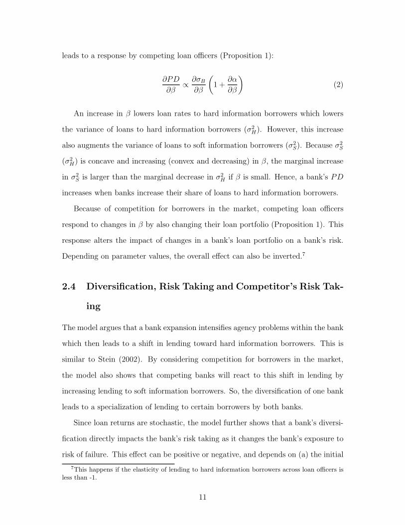
leads to a response by competing loan officers (Proposition 1):

∂PD

∂β∝

∂σB

∂β

(

1 +∂α

∂β

)

(2)

An increase in β lowers loan rates to hard information borrowers which lowers

the variance of loans to hard information borrowers (σ2H). However, this increase

also augments the variance of loans to soft information borrowers (σ2S). Because σ2

S

(σ2H) is concave and increasing (convex and decreasing) in β, the marginal increase

in σ2S is larger than the marginal decrease in σ2

H if β is small. Hence, a bank’s PD

increases when banks increase their share of loans to hard information borrowers.

Because of competition for borrowers in the market, competing loan officers

respond to changes in β by also changing their loan portfolio (Proposition 1). This

response alters the impact of changes in a bank’s loan portfolio on a bank’s risk.

Depending on parameter values, the overall effect can also be inverted.7

2.4 Diversification, Risk Taking and Competitor’s Risk Tak-

ing

The model argues that a bank expansion intensifies agency problems within the bank

which then leads to a shift in lending toward hard information borrowers. This is

similar to Stein (2002). By considering competition for borrowers in the market,

the model also shows that competing banks will react to this shift in lending by

increasing lending to soft information borrowers. So, the diversification of one bank

leads to a specialization of lending to certain borrowers by both banks.

Since loan returns are stochastic, the model further shows that a bank’s diversi-

fication directly impacts the bank’s risk taking as it changes the bank’s exposure to

risk of failure. This effect can be positive or negative, and depends on (a) the initial

7This happens if the elasticity of lending to hard information borrowers across loan officers isless than -1.

11

level of a bank’s loan portfolio, and (b) the response of competitors in the banking

market. Aside from this effect, a bank’s diversification activity also affects the risk

taking of competitors, even if they are not changing their level of diversification,

which happens because of the specialization on certain borrowers by competitors.

The theoretical framework shows that these effects can be positive or negative.

Therefore, I examine this relationship empirically using information from the U.S.

banking sector in the next section.

3 Diversification and Risk Taking

3.1 Empirical Strategy

In the empirical analysis I focus on differences in the level of geographic diversifica-

tion between banks and their competitors. Thus, I first determine for each bank in

a banking market its level of geographic diversification, Di,t. Averaging this value

within a banking market and excluding bank i from that calculation, allows me to

measure the average level of geographic diversity for bank i’s competitors (D−i,t).

Subtracting these two values from each other (D̄i,t = D−i,t − Di,t) then yields the

difference in the degree of diversification between bank i and its competitors. To

determine the relationship between this variable and bank i’s risk taking, I estimate

the following regression:

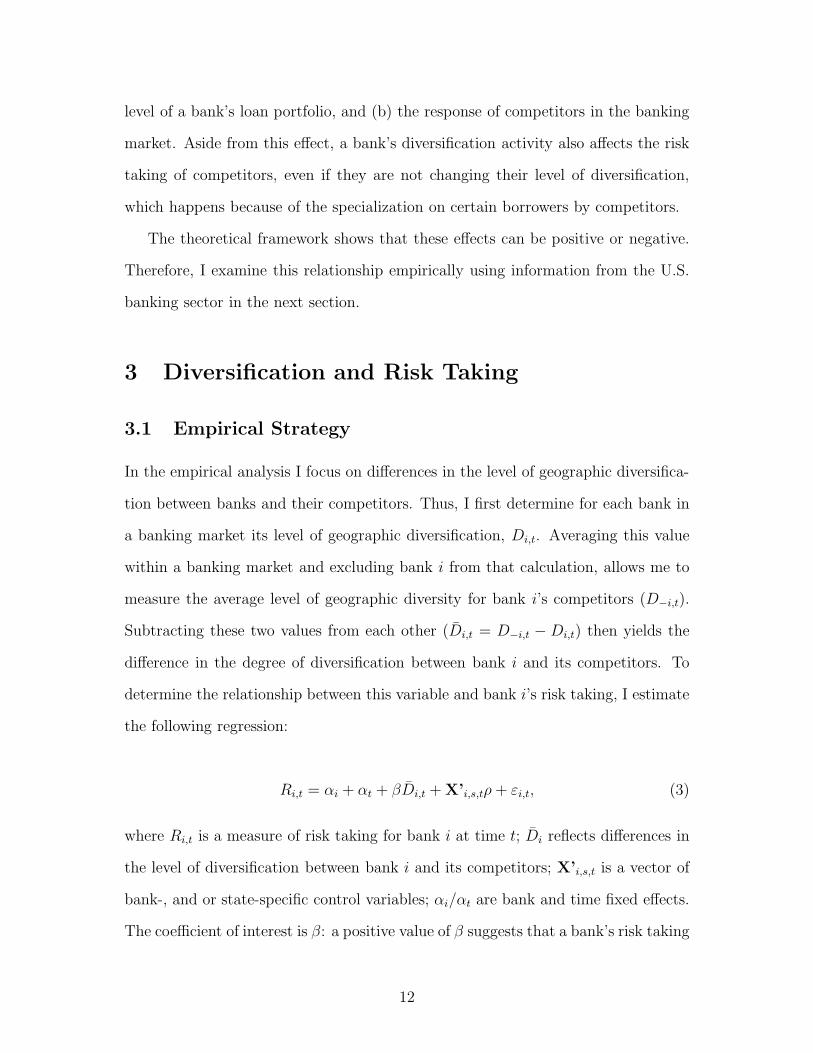
Ri,t = αi + αt + βD̄i,t +X’i,s,tρ+ εi,t, (3)

where Ri,t is a measure of risk taking for bank i at time t; D̄i reflects differences in

the level of diversification between bank i and its competitors; X’i,s,t is a vector of

bank-, and or state-specific control variables; αi/αt are bank and time fixed effects.

The coefficient of interest is β: a positive value of β suggests that a bank’s risk taking

12

increases as it becomes more diversified than its competitors. Similarly, a negative

value suggests that a bank’s risk taking decreases as its competitors increase their

relative level of geographic diversity.

3.2 Data

3.2.1 Sources

I use accounting data from commercial banks in the United States. These data come

from Reports of Condition and Income data (’Call Reports’), which all banking

institutions regulated by the Federal Deposit Insurance Corporation (FDIC), the

Federal Reserve, or the Office of the Comptroller of the Currency need to file on a

regular basis. I use semiannual data from the years 1976 to 2007 and only consider

commercial banks in the 50 states of the U.S. and the District of Columbia. The

geographical location of bank branches is recorded in the ‘Summary of Deposits’

which contains deposit data for branches and offices of all FDIC-insured institutions.

Aggregate state and county level data are from the Bureau of Economic Analysis.

3.2.2 Variable Definitions

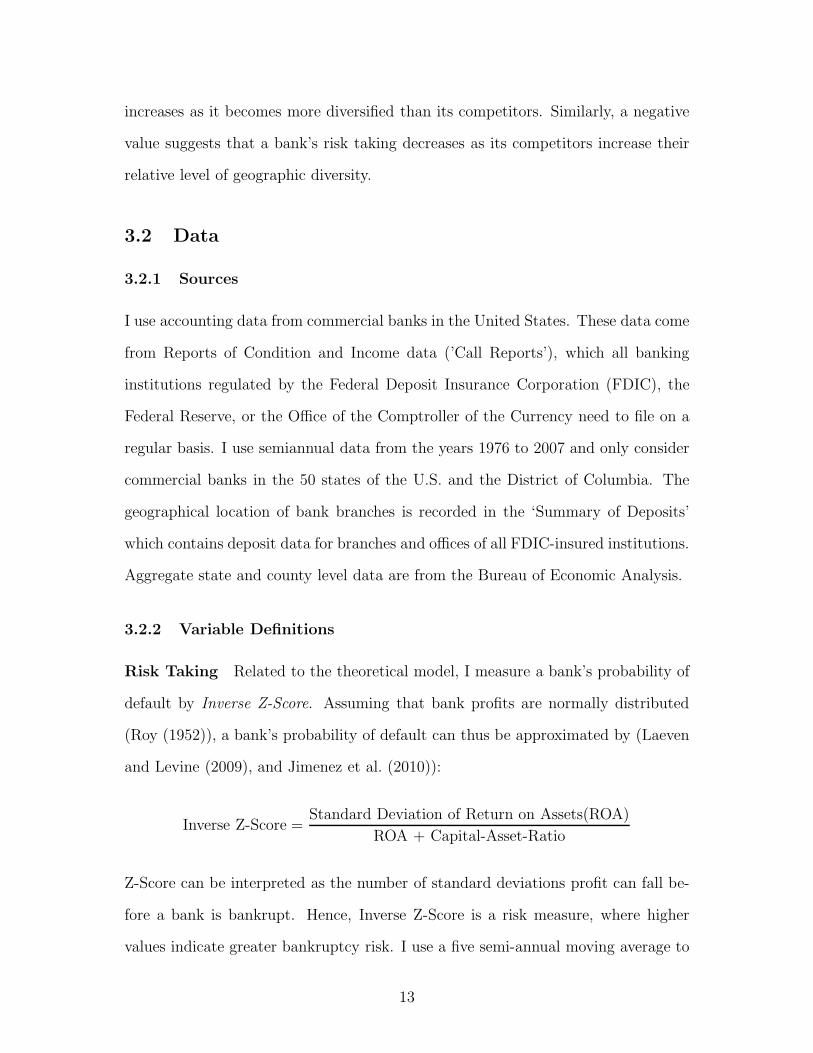
Risk Taking Related to the theoretical model, I measure a bank’s probability of

default by Inverse Z-Score. Assuming that bank profits are normally distributed

(Roy (1952)), a bank’s probability of default can thus be approximated by (Laeven

and Levine (2009), and Jimenez et al. (2010)):

Inverse Z-Score =Standard Deviation of Return on Assets(ROA)

ROA + Capital-Asset-Ratio

Z-Score can be interpreted as the number of standard deviations profit can fall be-

fore a bank is bankrupt. Hence, Inverse Z-Score is a risk measure, where higher

values indicate greater bankruptcy risk. I use a five semi-annual moving average to

13

estimate the volatility of profits using balance sheet information. To net out possible

time trends in return on assets (ROA) over the sample period, I subtract ROA from

its annual average.8 In addition to this variable, I construct a Distress indicator

which takes on the value of one whether a bank’s capital-asset ratio drops by more

than 1 % point in two consecutive years (Boyd et al. (2009)).9 Aside from this, I

also use balance sheet information and follow Laeven et al. (2002) to construct a

‘CAMEL’ rating for each bank and year.10 U.S. bank regulators evaluate the stabil-

ity of banks using balance sheet information and on-site inspections, and combine

their assessment in ‘CAMEL’ ratings, which range from 1 to 5, with higher ratings

indicating weaker banks. Because ‘CAMEL’ ratings are not publicly available, I fol-

low the methodology of Laeven et al. (2002) to construct them using balance sheet

information only.

Diversification I consider a U.S. county to be a relevant banking market for com-

mercial banks (Berger and Hannan (1989)), and hence I focus on banks’ expansion

into other counties within the same state. Morover, I do not focus on a bank’s

expansion within the same banking market, i.e. the opening of new branches in the

same county, and capture a bank’s structure across markets for each year by two

variables. The first variable is a Herfindahl Index of deposit concentration across

markets by summing up the squared share of deposits a bank has in each market.

This Herfindahl Index takes on values between zero and one, where larger values

indicate that a bank has a flatter organizational structure as it focuses on fewer

markets. I subtract this Herfindahl Index from one, so that smaller values of this

variable indicate a less diversified bank. Second, I compute for each bank and year

8This is equivalent to first estimating a year fixed regression of ROA, and then using theresiduals of ROA to compute Inverse Z-Score. The following OLS and 2SLS results also hold if Iuse reported ROA to determine Inverse Z-Score.

9I use the 1 % point threshold because it is the 10th percentile of the annual change in capital-asset ratio in my sample.

10CAMEL stands for Capital adequacy, Asset quality, Management quality, Earnings and Liq-uidity

14

the natural logarithm of banking markets, where I simply count the number of coun-

ties a bank has branches in. Lower values imply less geographic diversification as

they reflect that a bank is active in fewer markets.

For each bank and year, I determine the average of these two variables of all

banks that are active in the same market. Then, I take the average of each measure

in a county without including bank i and assign it to bank i, which yields for each

bank an average measure of bank i’s competitors’ diversification. Finally I subtract a

bank i’s measure of diversification from the average competitor’s degree to compute

D̄i,t (see equation (3)). This variable then captures relative differences between the

diversification of bank i and its competitors, where higher values indicate that the

competitors of bank i are relatively more diversified than bank i.

Controls To account for bank specific effects, I include the ratio of total loans to

total assets, the log of total assets, a dummy variable indicating whether the bank

is part of a bank holding company, and the capital-asset-ratio as control variables.

These variables are computed from balance sheet information for every bank and

year. State specific business cycle fluctuations are captured by the annual growth of

state personal income as well as a lag thereof. Since local banking market conditions

changed over the sample period, I include the log number of branches in a market,

log number of banks in market, the concentration of deposits across banks in a

market (Herfindahl Index) and population per branch in a market to account for

this.

3.2.3 Sample Characteristics

The U.S. banking sector also consists of several large banks that are active in more

than one state. The risk taking behavior of these banks is supposed to be different

than the behavior of banks that operate branches within state borders. Since I

15

am interested in the relationship between diversification and local competition, I

exclude banks that are active in more than one state. Additional details regarding

the construction of variables and the sample are given in the appendix.

The sample consists of 17,331 banks and spans the years 1977 to 2006. The

average bank size is $275 million, reflecting the fact that the U.S. banking sector

consists of many small banks and a few larger institutions. While the average return

on assets for banks in the sample is 0.57 %, banks are well capitalized with an average

capital-asset ratio of 9.23 %. Differences between diversified and nondiversified

banks are shown in Table 1. The majority of bank-year observations (about 83

%) are from nondiversified banks. This also reflects the fact that only 6 % of all

banks were diversified in 1977, whereas almost half of all banks in 2006 had at least

branches in two counties. Moreover, Table 1 suggests that diversified banks tend to

be (a) less risky, (b) larger, and (c) have lower capital-asset ratios.

3.3 Results

All regression models include bank fixed effects, which implies that the estimated

coefficient represents within bank changes in their risk taking behavior as a bank’s

competitors’ become more diversified than banks. Standard errors are robust and

clustered at the bank level. Results are presented in Table 2 and indicate that a

bank’s risk taking is negatively related to differences in the diversification of bank i

and its competitors even without conditioning on bank or macroeconomic controls.11

Moreover, the effect is significant at the 1 % level and robust to the inclusion of bank

and macroeconomic controls (column 2 and 3). The first two regression models in-

clude year fixed effects to account for unobservable time trends. However, these

fixed effects only capture unobservable time-varying effects at the country level.

Therefore I include region specific (column 4) or state-specific time dummies (col-

11Since Inverse Z-Score is small, I multiply it by 1,000 for my analysis.

16

umn 5) to capture unobservable time-varying effects on banks’ risk taking at the

region or state level.12 In particular, the state-specific time dummies capture unob-

servable effects such as changes in the competitive environment of commercial banks

at the state level. The relationship between banks’ diversification and risk taking is

significant at the 1 % level in all regression models.

To examine whether the results are sensitive to the definition of risk taking, I

repeat the analysis using the Distress Indicator or ‘CAMEL’ ratings as dependent

variable. I also include state-year fixed effects to account for unobservable charac-

teristics that vary within a state. Regression results are presented in Table 3 and

confirm the earlier findings as the results suggest that a bank’s risk taking is lower

when competitors become more diversified. Several banks exit the sample due to

mergers and acquisitions or failures. Although I include bank fixed effects in the

analysis, it is possible that a weeding out of risky banks (Carlson and Mitchener

(2009)) affects my findings. Therefore, I estimate the relationship between risk

taking and diversification excluding all banks that fail, merge or become acquired

during the sample period. The earlier findings are not driven by this and are robust

to this sample restriction. Similarly, banks also engage in mergers and acquisitions

during the sample period. This also affects the regression results. Specifically the

measure of risk taking, Inverse Z-Score, is affected as a merger or acquisition leads

to a re-evaluation of banks’ balance sheets. Therefore, I exclude observations one

year before to one year after a bank’s merger and/or acquisition (column 4), or all

observations after a bank engages in a merger or acquisition (column 5). While

the significance level drops, my earlier conclusions are not entirely driven by this.

Due to construction, Inverse Z-Score is correlated over time, as I use a five semester

moving average to estimate the volatility of bank profits. Hence, Inverse Z-Score in

12The regions are Midwest (IA, IL, IN, KS, MI, MN, MO, ND, NE, OH, WI), Northeast (CT,MA, MD, ME , NH, NJ, NY, PA, RI, VT, WV), South (AL, AR, DC, FL, GA, KY, LA, MS, NC,OK, SC, TN, TX, VA) and West (AZ, CA, CO, ID, MT, NM, NV, OR, UT, WA, WY).

17

year t uses information on profits that are also used for the computation of Inverse

Z-Score in year t− 1. Aside from this, persistence in earnings might also contribute

to a potential serial correlation of my risk measure. To address this, and virtually

eliminate all autocorrelation due to construction, I restrict the sample and only

include every third year in the estimation in column 6. The estimated coefficient

increases in magnitude and significance, suggesting that autocorrelation biases the

coefficient towards zero. Overall, these findings suggest that the relationship be-

tween diversification and risk taking is not driven by a bank’s merger activity or the

measurement of risk taking and diversification.

To translate these findings into a likelihood of failing, I estimate how a bank’s

probability of failing is related to Inverse Z-Score. Using information on the bankruptcy

of 1,152 bank failures during the sample period, I estimate a state and year fixed

effects logit regression and compute the average marginal effect of a one unit change

in Inverse Z-Score on a bank’s failure likelihood.13 Estimations from this logit model

suggest that a one unit increase in Inverse Z-score decreases the likelihood of failing

by approximately 1.2 %-points. Using the coefficient from column 4 in Table 2, I

find that if the difference between a bank’s competitors’ diversification and the di-

versity of a bank increases by one standard deviation, then the probability of failure

for a bank decreases by 0.6 basis points. During the sample period, on average three

out of a thousand banks fail each year, and so this implies that the average annual

failure rate would be reduced by approximately 2 %. This is a rather small effect.

However, it is a net effect and does not reflect the causal impact of diversification on

risk taking since causality is not identified in this Ordinary-least squares estimation.

13Because it is not possible to compute Inverse Z-Score in the last year of a bank’s existence, Idetermine for each bank whether it fails or not in the last period when Inverse Z-Score is available.

18

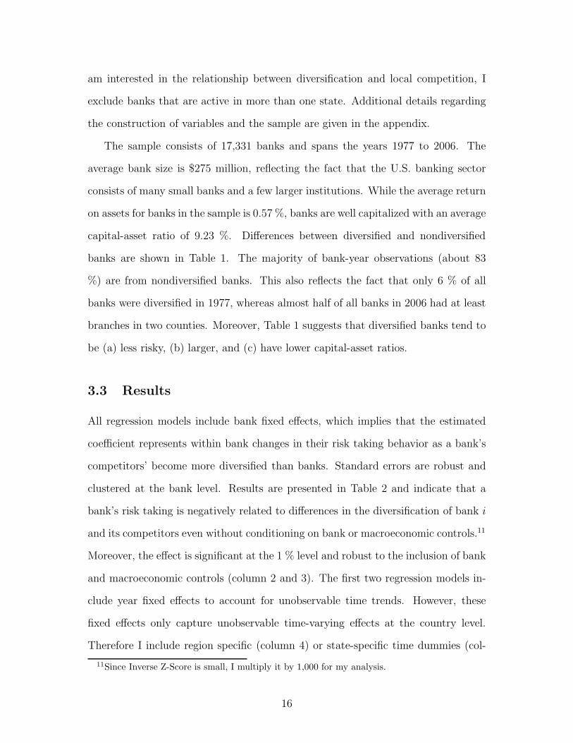
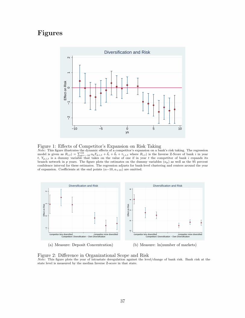
3.3.1 Dynamic effects

In 1977 about 5 % of all banks in the sample have branches in more than one

county. In 2006, on the other hand, almost every second bank has a branch network

that spans at least two counties. To examine the dynamic effects of risk taking as

competitors expand, I estimate the following regression model:

Ri,t = αi + αt +10∑

p=−10

βpYp,t +X’i,s,tρ+ εi,t

where Ri,t is the Inverse Z-Score of bank i in year t, Yp,t is a dummy variable

that takes on the value of one if in year t, bank i’s competitors diversify their

branch network across markets in p years. The effect on risk taking in the year

of the competitors’ expansion is dropped due to collinearity. Thus the coefficients

βp are relative to the year of competitors’ expansion. Figure 1 plots the estimated

coefficients βp as well as the 95 % confidence interval for these coefficients. To

account for a bank’s own diversification activity I restrict attention to banks that

are only active in a single market.

Figure 1 shows that a bank’s risk taking decreases once its competitors expand

their branch network into more markets. Furthermore, the figure shows that risk

taking does not significantly change before a competitor expands, and only decreases

significantly two years after a competitors expansion. This lagged response can

partly be attributed to the fact that Inverse Z-Score is smoothed as it is computed

using information from earlier years. The pattern in Figure 1 also shows that a

bank’s risk taking stays significantly lower once competitors diversified their branch

network into more markets, suggesting that the expansion of competitors has an

effect on a bank’s risk taking behavior.

19

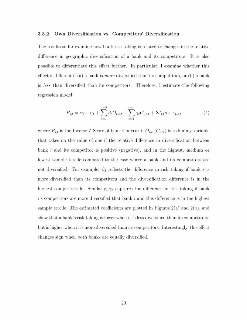
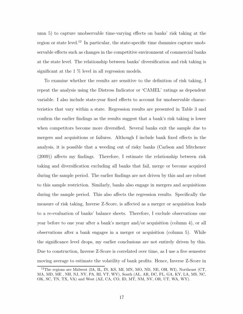
3.3.2 Own Diversification vs. Competitors’ Diversification

The results so far examine how bank risk taking is related to changes in the relative

difference in geographic diversification of a bank and its competitors. It is also

possible to differentiate this effect further. In particular, I examine whether this

effect is different if (a) a bank is more diversified than its competitors, or (b) a bank

is less than diversified than its competitors. Therefore, I estimate the following

regression model:

Ri,t = αi + αt +

e=3∑

e=1

βeOi,e,t +

e=3∑

e=1

γeCi,e,t +X’i,tρ+ εi,s,t (4)

where Ri,t is the Inverse Z-Score of bank i in year t, Oi,e (Ci,et) is a dummy variable

that takes on the value of one if the relative difference in diversification between

bank i and its competitor is positive (negative), and in the highest, medium or

lowest sample tercile compared to the case where a bank and its competitors are

not diversified. For example, β3 reflects the difference in risk taking if bank i is

more diversified than its competitors and the diversification difference is in the

highest sample tercile. Similarly, γ3 captures the difference in risk taking if bank

i’s competitors are more diversified that bank i and this difference is in the highest

sample tercile. The estimated coefficients are plotted in Figures 2(a) and 2(b), and

show that a bank’s risk taking is lower when it is less diversified than its competitors,

but is higher when it is more diversified than its competitors. Interestingly, this effect

changes sign when both banks are equally diversified.

20

4 The Effect of Diversification on Risk Taking:

2SLS

Ordinary-least squares estimation does not allow an identification of the causal re-

lationship between the effects of diversification on risk because of, for instance,

influences that jointly affect bank risk taking and diversification. To address this

concern, I employ two instrumental variable strategies. The first strategy uses the

timing of intrastate branching deregulation at the state level as an excluded in-

strument for the diversification activity of banks. The second approach combines

the timing of intrastate branching deregulation and bank specific characteristics in

a gravity-deregulation model similar to Frankel and Romer (1999) to develop an

instrumental variable at the bank level.

4.1 Intrastate Branching Deregulation as a Natural Exper-

iment

Banks in the United States were restricted in their branching decision within and

across states for many decades. Limits on the location of branch offices were imposed

in the 19th century, and were supported by the argument that allowing banks to

expand freely could lead to a monopolistic banking system. The granting of bank

charters was also a profitable income source for states, increasing incentives for

states to enact regulatory policies.14 These regulations led to a banking system that

was characterized by local monopolies within states since geographical restrictions

prohibited other banks from entering a market. Because banks were beneficiaries of

this regulation, they also had an incentive to preserve the status quo (Kroszner and

Strahan, 1999).

14How severe these restrictions were shows the case of Illinois: before the removal of theserestrictions, the state allowed banks to only open two branches within 3,500 yards of its mainoffice (Amel and Liang, 1992).

21

With the emergence of new technologies - such as the Automated Teller Machines

and more advanced credit scoring techniques - banks’ benefits from regulation de-

clined. Eventually intrastate branching restrictions were lifted in states, and banks

were allowed to branch freely within a state. The passage of the Riegle-Neal Act in

1994 by U.S. Congress finally removed all remaining barriers by the middle of the

1990s.15

The first stage regression model is given as:

D̄i,t = αi + αt + γZi,s,t +X’i,s,tρ+ εi,t, (5)

where D̄i,t is the relative level of geographic diversity between bank i and its com-

petitors, and larger values of D̄i,t indicate that competing banks are more diversified

than bank i; Zi,s,t is an instrumental variable, based on (1) the timing of intrastate

branching deregulation, or on (2) a gravity-deregulation model; X’i,s,t is a vector of

bank-, and or state-specific control variables; αi/αt are bank and time fixed effects.

In the second stage, I use the predicted value of D̄i,t to determine how it impacts

a banks’ risk taking.

Ri,t = β ˆ̄Di,t +X’i,s,tγ + δ̃i + δ̃t + ηi,s,t, (6)

where ˆ̄Di,t is the predicted value of the relative level of diversification between a bank

and its competitors from the first stage regression. I use the same data sources as

in the earlier analysis. Following previous research on intrastate branching deregu-

lation, I drop Delaware and South Dakota from the analysis since the structure of

the banking system in these states was heavily affected by other laws. Therefore it

is not possible to isolate the effect of intrastate branching deregulation in these two

15Previous research on intrastate branching deregulation suggests that the removal of branchingrestrictions had significant effects on the real activity and economic development. See among othersJayaratne and Strahan, 1996, Beck et al., 2010. Dates for each state are given in Table B.II.

22

states.

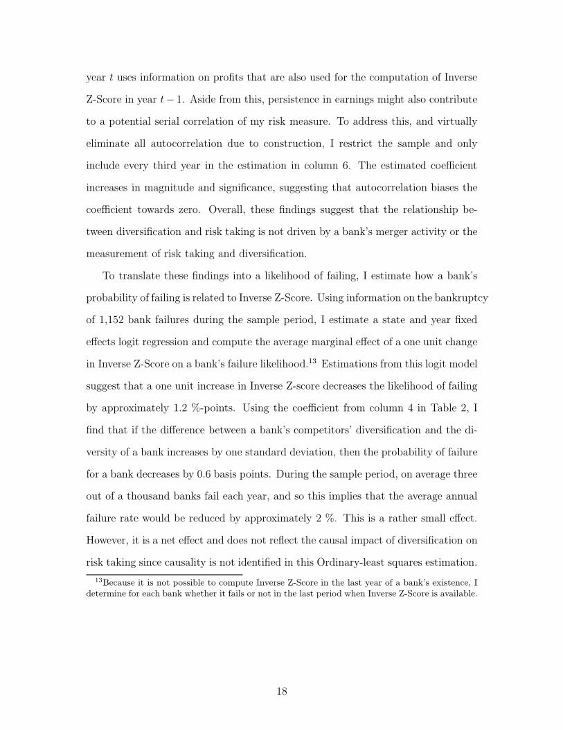
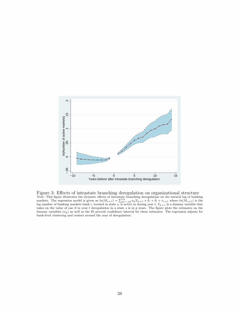
4.2 State-level instruments

4.2.1 Intrastate Branching Deregulation and Diversification

Intrastate branching restrictions prohibited banks from expanding their branch net-

work for many years. Figure 3 shows the dynamic effects of intrastate branching

deregulation in a state on the log number of markets a bank is active in. In partic-

ular, I estimate the following regression model:

ln(Mi,t) = αi + αt +

15∑

p=−10

βpYp,s,t + εi,t

where ln(Mi,t) is the log number of banking markets bank i is active in during

year t, Yp,s,t is a dummy variable that takes on the value of one if in year t, state s

liberalizes its intrastate branching restriction in p years. The effect on diversification

in the year of deregulation Y0,s,t is dropped due to collinearity; the coefficients βp are

relative to the year of intrastate branching deregulation. Figure 3 plots the estimated

coefficients βp as well as the 95 % confidence interval for these coefficients. The figure

indicates that, following the removal of branching restrictions, banks continuously

expand their branch network into more counties. Furthermore, a bank’s expansion

tendency is stronger in earlier years following intrastate branching deregulation, and

then slows down.

The instrumental variables for the 2SLS analysis are motivated by this finding,

and are based on the following four sets of time-varying, state-level instruments.

First, I use a dummy variable taking on the value of one once a state liberalized its

branching restrictions, and zero otherwise. While this indicator captures the average

effect of intrastate branching deregulation on a bank’s geographic diversification, it

does not capture changes over time. Therefore, I also use the number of years since a

23

state first started to remove its intrastate branching restrictions, and a square term

to allow for a quadratic relationship.16 Third, I employ a nonparametric specification

that includes independent dummy variables for each year since a state removed its

branching restrictions, taking a value of one all the way through the first ten years

after deregulation, and zero otherwise. Lastly, I use the natural logarithm of one

plus the number of years since a state removed its intrastate branching restrictions.

To isolate the effect of bank’s own expansion activity during the sample period,

I restrict attention to observations where banks are not diversified and therefore

only operate branches in one county. ˆ̄Di,t is thus measured relative to a nondiver-

sified bank i and thus captures the diversification activity of bank i’s competitors.

Furthermore, I exclude observations one year before and after a bank’s merger or

acquisition to account for changes in my risk measure due to merger activity. First

stage regression results of these instruments on competitors’ expansion across mar-

kets are presented in Panel B of Table 4. Similar to Figure 3, results in Table

4 indicate that intrastate branching deregulation is associated with an increase in

the diversification of banks as measured by the Herfindahl Index of deposits across

banking markets (columns 1 to 4). This also holds when I measure a bank’s diver-

sification using the log number of markets a bank is active in (columns 5 to 8). The

associated F-statistics support the use of these instruments as F-test results show

that intrastate branching deregulation significantly impacts the expansion of banks.

4.2.2 Diversification and Risk Taking: Second-stage

As mentioned before, I restrict attention to banks that are not geographically diver-

sified and also exclude observations around the year when banks engage in a merger

and/or acquisition. Hence, the measure of relative diversification reflects changes

in a competitors degree of geographic diversity. Panel A of Table 4 reports second

16Since Figure 3 shows that banks’ expansion decreases over time, I only allow for a linear andquadratic trend up to ten years after deregulation.

24

stage results of a 2SLS regression of bank risk on the level of geographic diversifica-

tion of competing banks, as measured by the competitor’s average dispersion across

markets (columns 1 to 4), or the average number of markets competitors are active

in (columns 5 to 8).

The results indicate that bank risk decreases significantly when competitors ex-

pand their diversification across markets. This effect is not sensitive to the defini-

tion of banks’ diversification, since I also find a statistically significant relationship

between competitors’ diversification and risk when I use the number of markets,

competitors are active in (columns 5 to 8). Moreover, I also find that the effect

between competitors’ diversification and risk taking is not sensitive to the definition

of risk since I find a statistically significant relationship between risk taking and

diversification when I measure risk taking using the Distress indicator or ‘CAMEL’

ratings.17 Compared to the OLS results (Table 2), the estimated coefficients from

the 2SLS analysis are larger in magnitude. This suggests an attenuation bias due

to reverse causality which results in smaller OLS estimates. The instrumental vari-

ables, however, allow me to identify a causal impact of changes in competitors’

diversification on banks’ risk taking.

Using the estimated coefficient reported in column 4 of Panel A of Table 4, I

compute that if competitors increase their dispersion across markets by one stan-

dard deviation, a bank’s probability of failure decreases by about 6 basis points.

Since the average annual failure rate of banks is 30 basis points, this implies that

a bank’s annual risk of bankruptcy decreases by 20 % when competitors increase

their diversity by one standard deviation.

17These results are unreported and are available upon request.

25

4.3 Gravity-Deregulation Model

Instrumental variables at the state-level are not able to capture a bank’s decision

to expand into other markets, and hence only provide an instrument for the aver-

age expansion of banks within a state. Moreover, unobservable state specific time

varying effects, such as a state’s overall level of bankruptcy risk, might influence my

findings.

Therefore, I design a strategy to differentiate the effect of a removal of branching

restrictions on banks’ expansion, which allows me to (1) account for the endogenous

choice of banks to expand within a state, and (2) include state specific time fixed ef-

fects to capture unobservable changes within a state. This approach incorporates (a)

the timing of intrastate branching deregulation at states, (b) the distance of coun-

ties within a state, and (c) differences between banks in regards to their regulatory

charter and/or membership to the Federal Reserve System.

4.3.1 Gravity-Deregulation Model: Strategy

Frankel and Romer (1999) devise an identification strategy using a gravity model

to analyze whether international trade causes economic growth. They determine

the effect of several country specific variables on trade flows between countries and

construct projected aggregate trade volumes at the country level. In a second step,

they use these constructed trade volumes as instruments for actual trade to iden-

tify the causal impact of trade on economic growth. Goetz et al. (2011) modify this

approach to pin down the causal relationship between a bank holding company’s ge-

ographic diversification across states in the United States and its market valuation.

To do so, they incorporate the state specific process of a removal of (bilateral) inter-

state banking restrictions in a gravity model to create an instrument that captures

a bank holding company’s level of geographic diversification.

Building upon their approach, I construct a bank-specific instrumental variable,

26

based on the timing of intrastate branching deregulation, the distance of counties

in a state, and bank specific characteristics. Specifically, I estimate the effect of

distance of a bank’s home county and another county on the degree of a bank’s

expansion into that county. Furthermore, I estimate how that effect changes once

states remove their intrastate branching restrictions. In particular, I hypothesize

that a bank’s share of deposits is larger in counties that are closer to the bank’s

home county. Moreover, I expect that the effect of distance on a bank’s expansion

into another county decreased once states removed intrastate branching restrictions.

Additionally, I examine how the relationship between expansion and distance

is different across bank types. In particular, I hypothesize that the link between

expansion and distance differs by (1) a bank’s charter authority (state or national

charter) and (2) a bank’s membership to the Federal Reserve System. Because

of the McFadden Act of 1927 and the Banking Act of 1933, banks in the U.S.

are subject to state specific banking laws irrespective of their charter type. Aside

from smaller differences, a bank’s charter choice determines its primary regulatory

agency, which can be associated with additional costs: state chartered banks are

supervised by state banking regulators and do not need to bear any costs due to

supervision. National chartered banks, on the other hand, are supervised by the

Office of the Comptroller of the Currency (OCC), which charges supervisory fees

(Blair and Kushmeider (2006)). Anecdotal evidence also suggests, that banks choose

state charters because state regulators, in contrast to national regulators, have a

better understanding of a bank’s business model in light of the local economy.18

Hence, a bank’s charter choice is supposed to reflect its desire to expand within

state borders once states liberalize intrastate branching restrictions.

Aside from this, banks can also decide whether they want to become members

of the Federal Reserve System. While national chartered banks are members of

18See for instance http : //www.arkansas.gov/bank/benefits why.html

27

the Federal Reserve System by default, state chartered banks can apply for mem-

bership. The Federal Reserve bank of the bank’s district decides whether to grant

membership, and evaluates the bank’s application based on factors such as, financial

condition or general character of management. Membership to the Federal Reserve

System provides banks with additional benefits, such as, for instance, the privilege

of voting for directors of the Federal Reserve bank. However, membership to the

Federal Reserve System is also costly, as it requires banks to subscribe to the capi-

tal stock in the Federal Reserve bank of its district. Moreover, once state chartered

banks are members of the Federal Reserve System, they are jointly supervised by

the Federal Reserve and state banking regulators - although at no additional costs

due to supervision.

Given these differences across bank types, I hypothesize that a removal of branch-

ing restrictions has different effects on banks’ branching decisions. Compared to

state chartered banks, I hypothesize that the effect of distance on expansion changes

more for national chartered banks once states remove their branching restrictions.

Similarly, I hypothesize that - compared to non-member banks - member banks of

the Federal Reserve System have a greater incentive to expand once states liberalize

their branching restrictions, implying that distance becomes less important once

branching restrictions are removed.

4.3.2 Zero-Stage: Distance and Intrastate Branching Deregulation

The following gravity-deregulation model estimates the effect of distance and size

on the expansion of banks within state borders:

Sharei,h,c,t = α1 ln(disth,c) + α2 ln(disth,c)×Bi,t +

+ α3 ln(disth,c)× Bi,t × Ii + α4 ln(disth,c)× Ii +∆i,h,c,t + εi,h,c,t,

28

where Sharei,h,c,t is the share of deposits bank i, headquartered in county h,

holds in branches in county c in year t; disth,c is the distance (in miles) between

county h and county c; Bi,t is a dummy variable taking on the value of one whether

bank i’s state removed its intrastate branching restrictions, or zero otherwise; Ii is

an indicator variable taking on the value of one, (1) whether bank i had a national

charter prior to intrastate branching deregulation, (2) and/or was a member of the

Federal Reserve System prior to intrastate branching deregulation, or zero otherwise;

∆i,h,c,t is a set of dummy variables accounting for fixed effects at the bank, county

and year level.

The baseline effect of distance on banks’ expansion is captured by the coefficient

α1. Changes of this relationship due to a removal of intrastate branching restrictions

are reflected in α2. Differential effects because of banks’ charter type or their mem-

bership to the Federal Reserve System are captured by α3. As mentioned above,

I hypothesize that banks have less deposits in branches that are further away, i.e.

α1 < 0, but I expect this effect to be mitigated once states liberalize branching

restrictions, i.e. α2 > 0. Furthermore, I expect that the effect of distance on ex-

pansion decreases more for national banks or Federal Reserve member banks once

states remove intrastate branching prohibitions.

Table 5 presents results from an OLS estimation of the gravity-deregulation

model where I use the share of deposits in % points as the dependent variable.19

The results show that banks have a smaller share of deposits in counties that are

further away from the county where they are headquartered in. As hypothesized, the

effect of distance on the share of deposits becomes smaller once states remove their

branching restrictions. This also holds when I include bank fixed effects (column 2).

In columns (3) to (5), I include the aforementioned bank specific variables. Results

in Table 5 suggest that distance is less important for a bank’s expansion if the bank

19Due to the size of the data set, I demeaned the dependent and independent variables by handto capture the reported fixed effects. Standard errors are robust and clustered at the bank level.

29

is a member of the Federal Reserve System and/or has a national charter.

The bank specific heterogeneity in the effect of distance on banks’ expansion

within states allows me to construct a projected expansion for each bank and year.

To be consistent with my earlier analysis, I estimate the gravity-deregulation model

where I use as dependent variable (1) an indicator taking on the value of one whether

bank i has a branch in county c in year t, and (2) the squared share of deposits

bank i holds in county c in year t. The projected variables are then aggregated at

the bank-year level to construct instrumental variables for (1) a bank’s number of

active banking markets, and (2) a bank’s deposit dispersion across markets. Similar

to before, I construct instruments for competitors’ expansion by taking the average

of each variable in a county without including bank i and assigning it to bank i.

Similar to the variable construction earlier, the projected relative difference in the

degree of geographic diversity is given by the difference between these two values.

4.3.3 Diversification and Risk Taking: Second-stage

Table 6 presents second stage regression results using instrumental variables based

on the gravity-deregulation model. In particular, I use the gravity models of column

4 in Table 5 to construct instruments for a bank’s level of geographic diversity and

the diversity of its competitors. Because the gravity-deregulation model allows me to

account for a bank’s own diversification activity, I include all bank-year observations

in my analysis.

Consistent with earlier findings, results in Table 6 indicate that banks’ risk taking

decreases when the relative difference in diversification between banks and their

competitors increases. This is not sensitive to the definition of diversification as I

find a statistically significant effect between diversification and risk taking when I

use the difference between a bank’s dispersion of deposits across counties and the

deposit dispersion of a bank’s competitors’ (column 1) or the difference in their

30

number of markets (column 2). Because the gravity-deregulation model provides an

instrumental variable at the bank level, I can separately identify (a) the impact of

a bank’s own level of diversification on its risk taking behavior and (b) the impact

of a bank’s competitors’ changes in diversification on risk taking. The findings in

Table 6 suggest that risk taking significantly increases when a bank diversifies its

activity across markets, consistent with earlier work by Demsetz and Strahan (1997).

However, when competitors increase their level of diversification across counties,

a bank’s risk taking significantly decreases. This pattern is consistent with the

theoretical model since the model shows that the effect of a bank’s diversification

on its own exposure to risk of failure is different than the effect of competing banks’

risk. Moreover, this finding is not sensitive to the definition of diversification as

it also holds when I use the number of markets, a bank is active in to capture its

degree of diversification. Furthermore, I also include state-year fixed effects in Table

6. These fixed effects capture unobservable, time-varying changes at the state level

and hence account for other confounding effects at the state level, such as changes

in overall bankruptcy risk at the state.

5 Conclusion

I present a theoretical model building on earlier work from Stein (2002) and Acharya

et al. (2011), to show how a bank’s diversification not only affects its own risk taking

behavior, but also the risk taking behavior of competing banks. In particular, the

model argues that a greater degree of geographic diversification has not only an

effect on a bank’s exposure to risk of failure, but also - due to competition for

borrowers in the market - an effect on competing bank’s risk taking.

To examine this pattern empirically, I analyze the relationship between diver-

sification and risk taking empirically using data from U.S. commercial banks and

31

find evidence consistent with this model. OLS regression results indicate that the

level of competitors’ degree of diversification is significantly correlated with bank’s

risk taking behavior. Moreover, I use the staggered timing of intrastate branching

deregulation, and a gravity-deregulation model to pin down the causal relation-

ship of banks’ diversification on risk taking of competing banks. Regression results

indicate that banks decrease risk taking when competitors increase their branch net-

work across counties or when their dispersion of deposits across markets changes.

My results also indicate that a bank’s own risk taking increases when it diversi-

fies across markets. Hence, these findings suggest that there are indirect effects of

diversification, as a bank’s risk taking is also affected as competitors change their

diversification.

32

References

Acharya, V. V., S. C. Myers, and R. G. Rajan (2011): “The Internal Gov-

ernance of Firms,” Journal of Finance, 66, 689–720.

Amel, D. and N. Liang (1992): “The Relationship between Entry into Banking

Markets and Changes in Legal Restrictions on Entry,” Antitrust Bulletin, 631 –

649.

Beck, T., R. Levine, and A. Levkov (2010): “Big Bad Banks: The Winners

and Losers from Bank Deregulation in the United States,” Journal of Finance,

65, 1637 – 1667.

Berger, A. N. and T. H. Hannan (1989): “The Price-Concentration Relation-

ship in Banking,” The Review of Economics and Statistics, 291 – 299.

Berger, A. N., N. H. Miller, M. A. Petersen, R. G. Rajan, and J. C.

Stein (2005): “Does function follow organizational form? Evidence from the

lending practices of large and small banks,” Journal of Financial Economics, 76,

237–269.

Blair, C. E. and R. M. Kushmeider (2006): “Challenges to the Dual Banking

System: The Funding of Bank Supervision,” FDIC Banking Review, 18, 1 – 22.

Boot, A. W. A. and A. Schmeits (2000): “Market Discipline and Incentive

Problems in Conglomerate Firms with Applications to Banking,” Journal of Fi-

nancial Intermediation, 9, 240 – 273.

Boyd, J. H. and G. de Nicolo (2005): “The Theory of Bank Risk Taking and

Competition Revisited,” Journal of Finance, 60, 1329–1343.

Boyd, J. H., G. de Nicolo, and A. M. Jalal (2007): “Bank Risk-Taking and

33

Competition Revisited: New Theory and New Evidence,” IMF working paper

WP/06/297.

Boyd, J. H., G. de Nicolo, and E. Loukoianova (2009): “Banking Crises

and Crisis Dating: Theory and Evidence,” IMF working paper WP/09/141.

Calomiris, C. W. and J. R. Mason (2000): “Causes of U.S. Bank Distress

during the depression,” NBER working paper 7919.

Carlson, M. and K. J. Mitchener (2009): “Branch Banking as a Device for

Discipline: Competition and Bank Survivorship during the Great Depression,”

Journal of Political Economy, 117, 165–210.

de Nicolo, G. (2000): “Size, charter value and risk in banking: an international

perspective,” Board of Governors of the Federal Reserve System, International

Finance Discussion Paper No.689.

Dell’Ariccia, G. and R. Marquez (2004): “Information and bank credit allo-

cation,” Journal of Financial Economics, 72, 185–214.

——— (2010): “Risk and the Corporate Structure of Banks,” Journal of Finance,

65, 1075–1096.

Demsetz, R. S. and P. E. Strahan (1997): “Diversification, Size, and Risk at

Bank Holding Companies,” Journal of Money, Credit, and Banking, 29, 300–313.

Diamond, D. (1984): “Financial intermediation and delegated monitoring,” Review

of Economic Studies, 51, 393–414.

Frankel, J. A. and D. Romer (1999): “Does Trade Cause Growth?” American

Economic Review, 89, 379–399.

Goetz, M., L. Laeven, and R. Levine (2011): “The Valuation Effects of Geo-

graphically Diversified Bank Holding Companies,” Mimeo.

34

Hertzberg, A., J. M. Liberti, and D. Paravisini (2010): “Information and

Incentives Inside the Firm: Evidence from Loan Officer Rotation,” Journal of

Finance, 65, 795–828.

Jayaratne, J. and P. E. Strahan (1996): “The Finance-Growth Nexus: Ev-

idence from Bank Branch Deregulation,” Quarterly Journal of Economics, 111,

639–670.

Jimenez, G., J. A. Lopez, and J. Saurina (2010): “How does Competition

Impact Bank Risk-Taking?” Mimeo, Banco de Espana.

Keeley, M. C. (1990): “Deposit Insurance, Risk, and Market Power in Banking,”

American Economic Review, 80, 1183–1199.

Kroszner, R. S. and P. E. Strahan (1999): “What Drives Deregulation? Eco-

nomics and Politics of the Relaxation of Bank Branching Restrictions,” Quarterly

Journal of Economics, 114, 1437–1467.

Laeven, L., P. Bongini, and G. Majnoni (2002): “How Good is the Market at

Assessing Bank Fragility? A Horse Race Between Different Indicators,” Journal

of Banking and Finance, 26, 1011–1028.

Laeven, L. and R. Levine (2009): “Bank governance, regulation and risk tak-

ing,” Journal of Financial Economics, 93, 259–275.

Liberti, J. M. and A. R. Mian (2009): “Estimating the Effect of Hierarchies on

Information Use,” The Review of Financial Studies, 22, 4057–4090.

Martinez-Miera, D. and R. Repullo (2010): “Does Competition Reduce the

Risk of Bank Failure?” Review of Financial Studies, 23, 3638–3664.

Mitchener, K. J. (2005): “Bank Supervision, Regulation, and Instability During

the Great Depression,” The Journal of Economic History, 65, 152–185.

35

Morgan, D. P. (2002): “Rating Banks: Risk and Uncertainty in an Opaque

Industry,” American Economic Review, 92, 874–888.

Morgan, D. P., B. Rime, and P. E. Strahan (2004): “Bank Integration and

State Business Cycles,” Quarterly Journal of Economics, 1555–1584.

Petersen, M. A. and R. G. Rajan (1995): “The Effect of Credit Market Compe-

tition on Lending Relationships,” Quarterly Journal of Economics, 110, 407–443.

Roy, A. (1952): “Safety First and the Holding of Assets,” Econometrica, 431–449.

Stein, J. C. (2002): “Information Production and Capital Allocation: Decentral-

ized versus Hierarchical Firms,” Journal of Finance, 57, 1891–1921.

36

Figures

−2

−1

01

2E

ffect

on

Ris

k

−10 −5 0 5 10ys

Diversification and Risk

Figure 1: Effects of Competitor’s Expansion on Risk TakingNote: This figure illustrates the dynamic effects of a competitor’s expansion on a bank’s risk taking. The regressionmodel is given as Ri,t) =

∑10p=−10 αpYp,i,t + δ̃i + δ̃t + τi,s,t where Ri,t) is the Inverse Z-Score of bank i in year

t, Yp,i,t is a dummy variable that takes on the value of one if in year t the competitor of bank i expands itsbranch network in p years. The figure plots the estimates on the dummy variables (αp) as well as the 95 percentconfidence interval for these estimates. The regression adjusts for bank-level clustering and centers around the yearof expansion. Coefficients at the end points (α−10, α+10) are omitted.

−1

01

2E

ffect

on

Ris

k

competitor less diversified competitor more diversified Competitors’ Diversification − Own Diversification

Diversification and Risk

(a) Measure: Deposit Concentration)

−2

02

46

Effe

ct o

n R

isk

competitor less diversified competitor more diversified Competitors’ Diversification − Own Diversification

Diversification and Risk

(b) Measure: ln(number of markets)

Figure 2: Difference in Organizational Scope and RiskNote: This figure plots the year of intrastate deregulation against the level/change of bank risk. Bank risk at thestate level is measured by the median Inverse Z-score in that state.

37

−.0

50

.05

.1.1

5.2

ln(N

umbe

r of

act

ive

mar

kets

)

−10 −5 0 5 10 15Years before/ after intrastate branching deregulation

Figure 3: Effects of intrastate branching deregulation on organizational structureNote: This figure illustrates the dynamic effects of intrastate branching deregulation on the natural log of bankingmarkets. The regression model is given as ln(Mi,s,t) =

∑15p=−10 αpYp,s,t + δ̃i + δ̃t + τi,s,t where ln(Mi,s,t) is the

log number of banking markets bank i, located in state s, is active in during year t, Yp,s,t is a dummy variable thattakes on the value of one if in year t deregulation in a state s is in p years. The figure plots the estimates on thedummy variables (αp) as well as the 95 percent confidence interval for these estimates. The regression adjusts forbank-level clustering and centers around the year of deregulation.

38

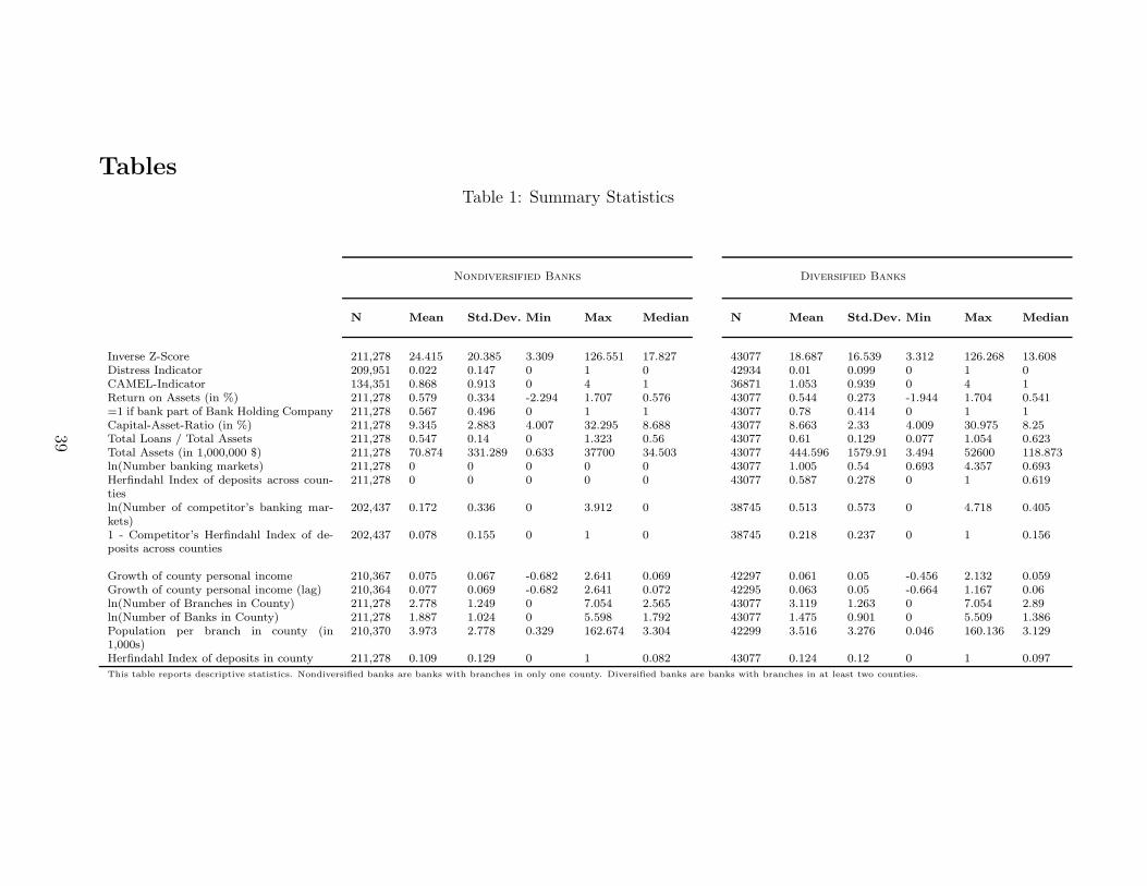
Table 1: Summary Statistics

Nondiversified Banks Diversified Banks

N Mean Std.Dev. Min Max Median N Mean Std.Dev. Min Max Median

Inverse Z-Score 211,278 24.415 20.385 3.309 126.551 17.827 43077 18.687 16.539 3.312 126.268 13.608Distress Indicator 209,951 0.022 0.147 0 1 0 42934 0.01 0.099 0 1 0CAMEL-Indicator 134,351 0.868 0.913 0 4 1 36871 1.053 0.939 0 4 1Return on Assets (in %) 211,278 0.579 0.334 -2.294 1.707 0.576 43077 0.544 0.273 -1.944 1.704 0.541=1 if bank part of Bank Holding Company 211,278 0.567 0.496 0 1 1 43077 0.78 0.414 0 1 1Capital-Asset-Ratio (in %) 211,278 9.345 2.883 4.007 32.295 8.688 43077 8.663 2.33 4.009 30.975 8.25Total Loans / Total Assets 211,278 0.547 0.14 0 1.323 0.56 43077 0.61 0.129 0.077 1.054 0.623Total Assets (in 1,000,000 $) 211,278 70.874 331.289 0.633 37700 34.503 43077 444.596 1579.91 3.494 52600 118.873ln(Number banking markets) 211,278 0 0 0 0 0 43077 1.005 0.54 0.693 4.357 0.693Herfindahl Index of deposits across coun-ties

211,278 0 0 0 0 0 43077 0.587 0.278 0 1 0.619

ln(Number of competitor’s banking mar-kets)

202,437 0.172 0.336 0 3.912 0 38745 0.513 0.573 0 4.718 0.405

1 - Competitor’s Herfindahl Index of de-posits across counties

202,437 0.078 0.155 0 1 0 38745 0.218 0.237 0 1 0.156

Growth of county personal income 210,367 0.075 0.067 -0.682 2.641 0.069 42297 0.061 0.05 -0.456 2.132 0.059Growth of county personal income (lag) 210,364 0.077 0.069 -0.682 2.641 0.072 42295 0.063 0.05 -0.664 1.167 0.06ln(Number of Branches in County) 211,278 2.778 1.249 0 7.054 2.565 43077 3.119 1.263 0 7.054 2.89ln(Number of Banks in County) 211,278 1.887 1.024 0 5.598 1.792 43077 1.475 0.901 0 5.509 1.386Population per branch in county (in1,000s)

210,370 3.973 2.778 0.329 162.674 3.304 42299 3.516 3.276 0.046 160.136 3.129

Herfindahl Index of deposits in county 211,278 0.109 0.129 0 1 0.082 43077 0.124 0.12 0 1 0.097

This table reports descriptive statistics. Nondiversified banks are banks with branches in only one county. Diversified banks are banks with branches in at least two counties.

Tables

39

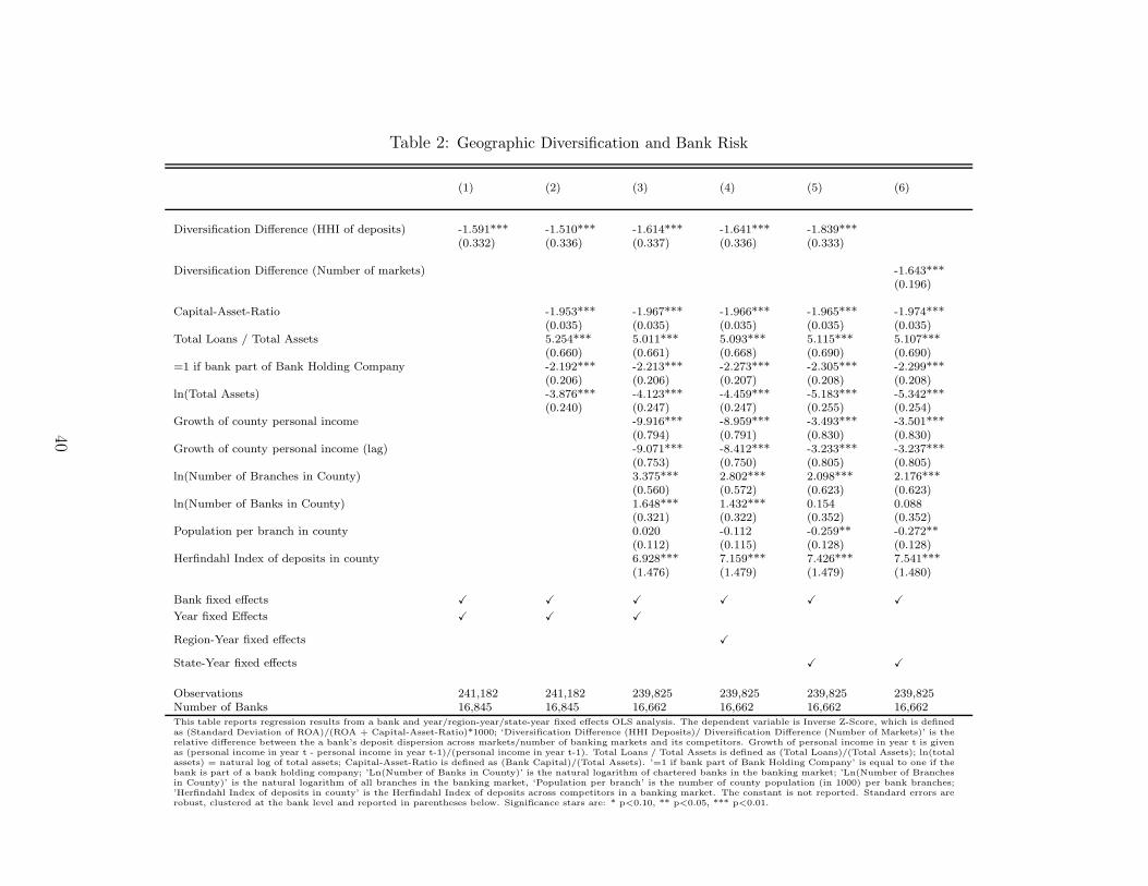
Table 2: Geographic Diversification and Bank Risk

(1) (2) (3) (4) (5) (6)

Diversification Difference (HHI of deposits) -1.591*** -1.510*** -1.614*** -1.641*** -1.839***(0.332) (0.336) (0.337) (0.336) (0.333)

Diversification Difference (Number of markets) -1.643***(0.196)

Capital-Asset-Ratio -1.953*** -1.967*** -1.966*** -1.965*** -1.974***(0.035) (0.035) (0.035) (0.035) (0.035)

Total Loans / Total Assets 5.254*** 5.011*** 5.093*** 5.115*** 5.107***(0.660) (0.661) (0.668) (0.690) (0.690)

=1 if bank part of Bank Holding Company -2.192*** -2.213*** -2.273*** -2.305*** -2.299***(0.206) (0.206) (0.207) (0.208) (0.208)

ln(Total Assets) -3.876*** -4.123*** -4.459*** -5.183*** -5.342***(0.240) (0.247) (0.247) (0.255) (0.254)

Growth of county personal income -9.916*** -8.959*** -3.493*** -3.501***(0.794) (0.791) (0.830) (0.830)

Growth of county personal income (lag) -9.071*** -8.412*** -3.233*** -3.237***(0.753) (0.750) (0.805) (0.805)

ln(Number of Branches in County) 3.375*** 2.802*** 2.098*** 2.176***(0.560) (0.572) (0.623) (0.623)

ln(Number of Banks in County) 1.648*** 1.432*** 0.154 0.088(0.321) (0.322) (0.352) (0.352)

Population per branch in county 0.020 -0.112 -0.259** -0.272**(0.112) (0.115) (0.128) (0.128)

Herfindahl Index of deposits in county 6.928*** 7.159*** 7.426*** 7.541***(1.476) (1.479) (1.479) (1.480)

Bank fixed effects X X X X X X

Year fixed Effects X X X

Region-Year fixed effects X

State-Year fixed effects X X

Observations 241,182 241,182 239,825 239,825 239,825 239,825Number of Banks 16,845 16,845 16,662 16,662 16,662 16,662This table reports regression results from a bank and year/region-year/state-year fixed effects OLS analysis. The dependent variable is Inverse Z-Score, which is definedas (Standard Deviation of ROA)/(ROA + Capital-Asset-Ratio)*1000; ‘Diversification Difference (HHI Deposits)/ Diversification Difference (Number of Markets)’ is therelative difference between the a bank’s deposit dispersion across markets/number of banking markets and its competitors. Growth of personal income in year t is givenas (personal income in year t - personal income in year t-1)/(personal income in year t-1). Total Loans / Total Assets is defined as (Total Loans)/(Total Assets); ln(totalassets) = natural log of total assets; Capital-Asset-Ratio is defined as (Bank Capital)/(Total Assets). ’=1 if bank part of Bank Holding Company’ is equal to one if thebank is part of a bank holding company; ’Ln(Number of Banks in County)’ is the natural logarithm of chartered banks in the banking market; ’Ln(Number of Branchesin County)’ is the natural logarithm of all branches in the banking market, ‘Population per branch’ is the number of county population (in 1000) per bank branches;’Herfindahl Index of deposits in county’ is the Herfindahl Index of deposits across competitors in a banking market. The constant is not reported. Standard errors arerobust, clustered at the bank level and reported in parentheses below. Significance stars are: * p<0.10, ** p<0.05, *** p<0.01.

40

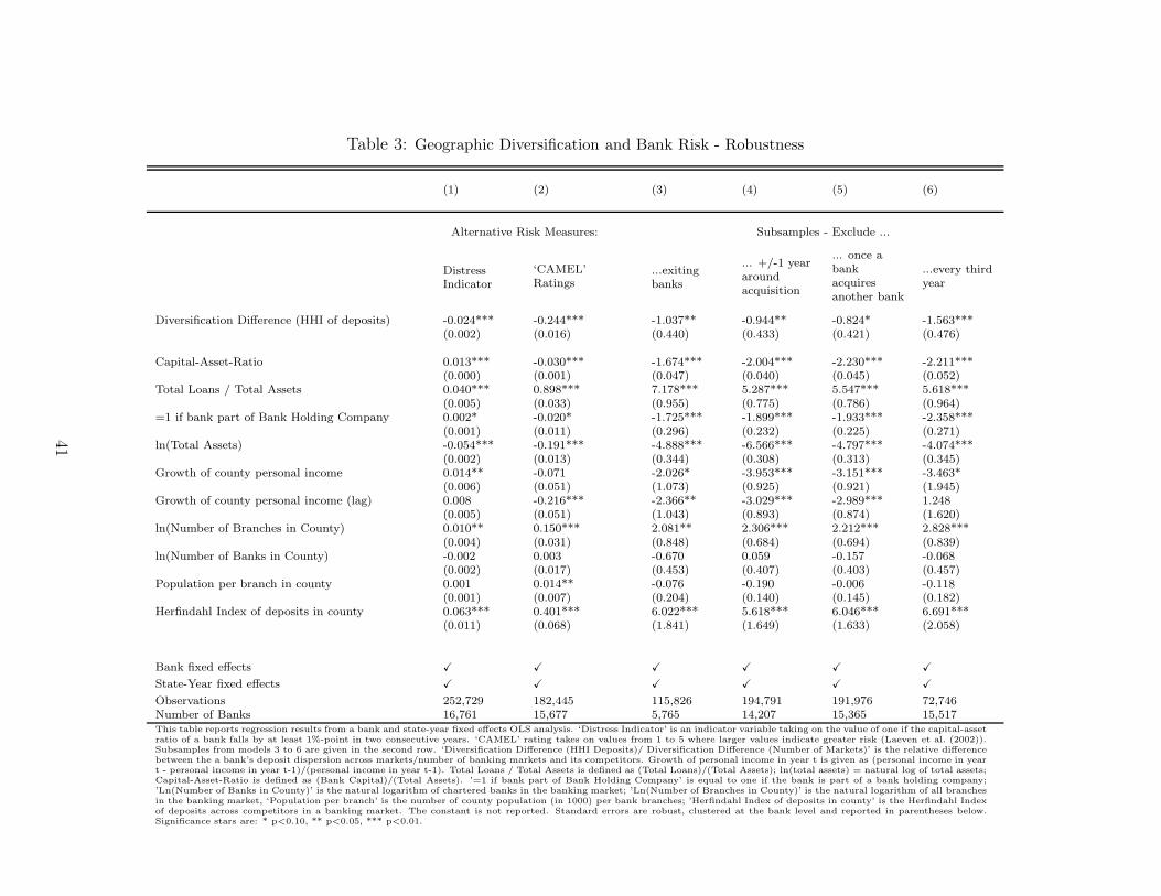
Table 3: Geographic Diversification and Bank Risk - Robustness

(1) (2) (3) (4) (5) (6)

Alternative Risk Measures: Subsamples - Exclude ...

DistressIndicator

‘CAMEL’Ratings

...exitingbanks

... +/-1 yeararoundacquisition

... once abankacquiresanother bank

...every thirdyear

Diversification Difference (HHI of deposits) -0.024*** -0.244*** -1.037** -0.944** -0.824* -1.563***(0.002) (0.016) (0.440) (0.433) (0.421) (0.476)

Capital-Asset-Ratio 0.013*** -0.030*** -1.674*** -2.004*** -2.230*** -2.211***(0.000) (0.001) (0.047) (0.040) (0.045) (0.052)

Total Loans / Total Assets 0.040*** 0.898*** 7.178*** 5.287*** 5.547*** 5.618***(0.005) (0.033) (0.955) (0.775) (0.786) (0.964)

=1 if bank part of Bank Holding Company 0.002* -0.020* -1.725*** -1.899*** -1.933*** -2.358***(0.001) (0.011) (0.296) (0.232) (0.225) (0.271)

ln(Total Assets) -0.054*** -0.191*** -4.888*** -6.566*** -4.797*** -4.074***(0.002) (0.013) (0.344) (0.308) (0.313) (0.345)

Growth of county personal income 0.014** -0.071 -2.026* -3.953*** -3.151*** -3.463*(0.006) (0.051) (1.073) (0.925) (0.921) (1.945)

Growth of county personal income (lag) 0.008 -0.216*** -2.366** -3.029*** -2.989*** 1.248(0.005) (0.051) (1.043) (0.893) (0.874) (1.620)

ln(Number of Branches in County) 0.010** 0.150*** 2.081** 2.306*** 2.212*** 2.828***(0.004) (0.031) (0.848) (0.684) (0.694) (0.839)

ln(Number of Banks in County) -0.002 0.003 -0.670 0.059 -0.157 -0.068(0.002) (0.017) (0.453) (0.407) (0.403) (0.457)

Population per branch in county 0.001 0.014** -0.076 -0.190 -0.006 -0.118(0.001) (0.007) (0.204) (0.140) (0.145) (0.182)

Herfindahl Index of deposits in county 0.063*** 0.401*** 6.022*** 5.618*** 6.046*** 6.691***(0.011) (0.068) (1.841) (1.649) (1.633) (2.058)

Bank fixed effects X X X X X X

State-Year fixed effects X X X X X X

Observations 252,729 182,445 115,826 194,791 191,976 72,746Number of Banks 16,761 15,677 5,765 14,207 15,365 15,517This table reports regression results from a bank and state-year fixed effects OLS analysis. ‘Distress Indicator’ is an indicator variable taking on the value of one if the capital-assetratio of a bank falls by at least 1%-point in two consecutive years. ‘CAMEL’ rating takes on values from 1 to 5 where larger values indicate greater risk (Laeven et al. (2002)).Subsamples from models 3 to 6 are given in the second row. ‘Diversification Difference (HHI Deposits)/ Diversification Difference (Number of Markets)’ is the relative differencebetween the a bank’s deposit dispersion across markets/number of banking markets and its competitors. Growth of personal income in year t is given as (personal income in yeart - personal income in year t-1)/(personal income in year t-1). Total Loans / Total Assets is defined as (Total Loans)/(Total Assets); ln(total assets) = natural log of total assets;Capital-Asset-Ratio is defined as (Bank Capital)/(Total Assets). ’=1 if bank part of Bank Holding Company’ is equal to one if the bank is part of a bank holding company;’Ln(Number of Banks in County)’ is the natural logarithm of chartered banks in the banking market; ’Ln(Number of Branches in County)’ is the natural logarithm of all branchesin the banking market, ‘Population per branch’ is the number of county population (in 1000) per bank branches; ’Herfindahl Index of deposits in county’ is the Herfindahl Indexof deposits across competitors in a banking market. The constant is not reported. Standard errors are robust, clustered at the bank level and reported in parentheses below.Significance stars are: * p<0.10, ** p<0.05, *** p<0.01.

41

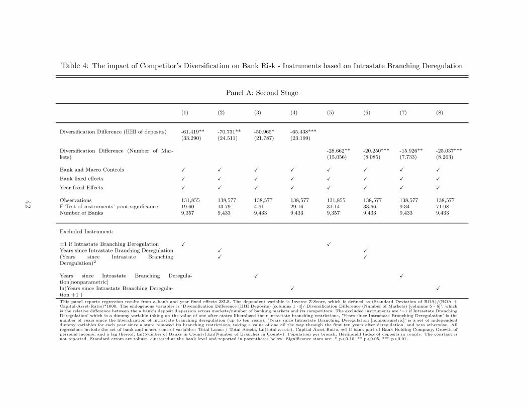
Table 4: The impact of Competitor’s Diversification on Bank Risk - Instruments based on Intrastate Branching Deregulation

Panel A: Second Stage

(1) (2) (3) (4) (5) (6) (7) (8)

Diversification Difference (HHI of deposits) -61.419** -70.731** -50.965* -65.438***(33.290) (24.511) (21.787) (23.199)

Diversification Difference (Number of Mar-kets)

-28.662** -20.250*** -15.926** -25.037***(15.056) (8.085) (7.733) (8.263)

Bank and Macro Controls X X X X X X X X

Bank fixed effects X X X X X X X X

Year fixed Effects X X X X X X X X

Observations 131,855 138,577 138,577 138,577 131,855 138,577 138,577 138,577F Test of instruments’ joint significance 19.60 13.79 4.61 29.16 31.14 33.66 9.34 71.98Number of Banks 9,357 9,433 9,433 9,433 9,357 9,433 9,433 9,433

Excluded Instrument:

=1 if Intrastate Branching Deregulation X X

Years since Intrastate Branching Deregulation X X

(Years since Intrastate BranchingDeregulation)2

X X

Years since Intrastate Branching Deregula-tion[nonparametric]

X X

ln(Years since Intrastate Branching Deregula-tion +1 )

X X

This panel reports regression results from a bank and year fixed effects 2SLS. The dependent variable is Inverse Z-Score, which is defined as (Standard Deviation of ROA)/(ROA +Capital-Asset-Ratio)*1000. The endogenous variables is ‘Diversification Difference (HHI Deposits) [columns 1 -4]/ Diversification Difference (Number of Markets) [columns 5 - 8]’, whichis the relative difference between the a bank’s deposit dispersion across markets/number of banking markets and its competitors. The excluded instruments are ‘=1 if Intrastate BranchingDeregulation’ which is a dummy variable taking on the value of one after states liberalized their intrastate branching restrictions, ’Years since Intrastate Branching Deregulation’ is thenumber of years since the liberalization of intrastate branching deregulation (up to ten years), ’Years since Intrastate Branching Deregulation [nonparametric]’ is a set of independentdummy variables for each year since a state removed its branching restrictions, taking a value of one all the way through the first ten years after deregulation, and zero otherwise. Allregressions include the set of bank and macro control variables: Total Loans / Total Assets, Ln(total assets), Capital-Asset-Ratio, =1 if bank part of Bank Holding Company, Growth ofpersonal income, and a lag thereof, Ln(Number of Banks in County),Ln(Number of Branches in County), Population per branch, Herfindahl Index of deposits in county. The constant isnot reported. Standard errors are robust, clustered at the bank level and reported in parentheses below. Significance stars are: * p<0.10, ** p<0.05, *** p<0.01.

42

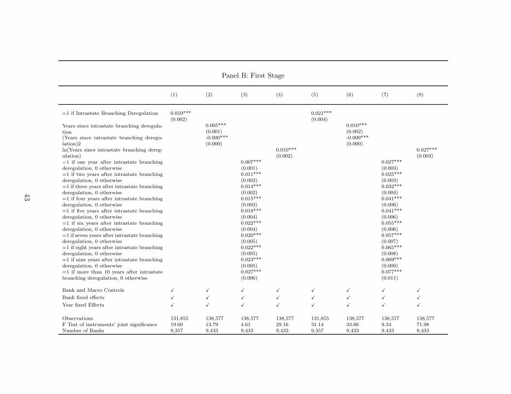
Panel B: First Stage

(1) (2) (3) (4) (5) (6) (7) (8)

=1 if Intrastate Branching Deregulation 0.010*** 0.021***(0.002) (0.004)

Years since intrastate branching deregula-tion

0.005*** 0.010***(0.001) (0.002)

(Years since intrastate branching deregu-lation)2

-0.000*** -0.000***(0.000) (0.000)

ln(Years since intrastate branching dereg-ulation)

0.010*** 0.027***(0.002) (0.003)

=1 if one year after intrastate branchingderegulation, 0 otherwise

0.007*** 0.027***(0.001) (0.003)

=1 if two years after intrastate branchingderegulation, 0 otherwise

0.011*** 0.025***(0.002) (0.003)

=1 if three years after intrastate branchingderegulation, 0 otherwise

0.014*** 0.032***(0.002) (0.004)

=1 if four years after intrastate branchingderegulation, 0 otherwise

0.015*** 0.041***(0.003) (0.006)

=1 if five years after intrastate branchingderegulation, 0 otherwise

0.018*** 0.041***(0.004) (0.006)

=1 if six years after intrastate branchingderegulation, 0 otherwise

0.022*** 0.055***(0.004) (0.006)

=1 if seven years after intrastate branchingderegulation, 0 otherwise

0.020*** 0.057***(0.005) (0.007)

=1 if eight years after intrastate branchingderegulation, 0 otherwise

0.022*** 0.065***(0.005) (0.008)

=1 if nine years after intrastate branchingderegulation, 0 otherwise

0.023*** 0.069***(0.005) (0.009)

=1 if more than 10 years after intrastatebranching deregulation, 0 otherwise

0.027*** 0.077***(0.006) (0.011)

Bank and Macro Controls X X X X X X X X

Bank fixed effects X X X X X X X X

Year fixed Effects X X X X X X X X

Observations 131,855 138,577 138,577 138,577 131,855 138,577 138,577 138,577F Test of instruments’ joint significance 19.60 13.79 4.61 29.16 31.14 33.66 9.34 71.98Number of Banks 9,357 9,433 9,433 9,433 9,357 9,433 9,433 9,433

43

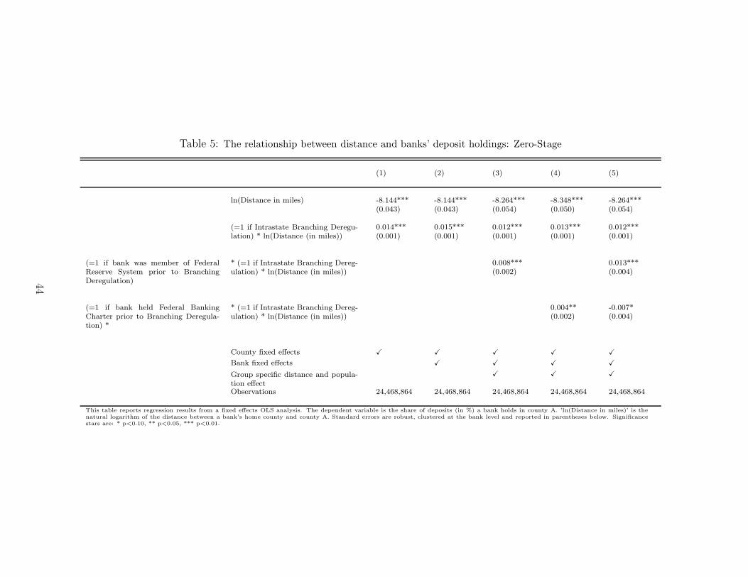
Table 5: The relationship between distance and banks’ deposit holdings: Zero-Stage

(1) (2) (3) (4) (5)

ln(Distance in miles) -8.144*** -8.144*** -8.264*** -8.348*** -8.264***(0.043) (0.043) (0.054) (0.050) (0.054)

(=1 if Intrastate Branching Deregu-lation) * ln(Distance (in miles))

0.014*** 0.015*** 0.012*** 0.013*** 0.012***(0.001) (0.001) (0.001) (0.001) (0.001)

(=1 if bank was member of FederalReserve System prior to BranchingDeregulation)

* (=1 if Intrastate Branching Dereg-ulation) * ln(Distance (in miles))

0.008*** 0.013***(0.002) (0.004)

(=1 if bank held Federal BankingCharter prior to Branching Deregula-tion) *

* (=1 if Intrastate Branching Dereg-ulation) * ln(Distance (in miles))

0.004** -0.007*(0.002) (0.004)

County fixed effects X X X X X

Bank fixed effects X X X X

Group specific distance and popula-tion effect

X X X

Observations 24,468,864 24,468,864 24,468,864 24,468,864 24,468,864

This table reports regression results from a fixed effects OLS analysis. The dependent variable is the share of deposits (in %) a bank holds in county A. ’ln(Distance in miles)’ is thenatural logarithm of the distance between a bank’s home county and county A. Standard errors are robust, clustered at the bank level and reported in parentheses below. Significancestars are: * p<0.10, ** p<0.05, *** p<0.01.

44

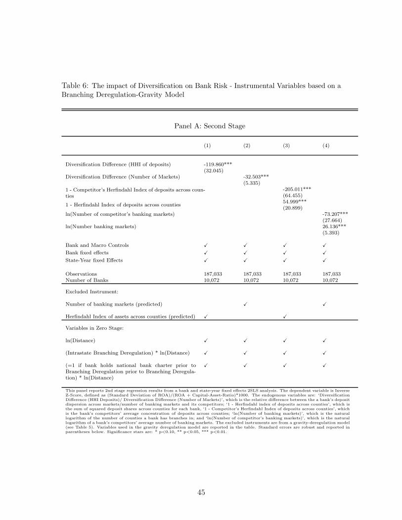
Table 6: The impact of Diversification on Bank Risk - Instrumental Variables based on aBranching Deregulation-Gravity Model

Panel A: Second Stage

(1) (2) (3) (4)

Diversification Difference (HHI of deposits) -119.860***(32.045)

Diversification Difference (Number of Markets) -32.503***(5.335)

1 - Competitor’s Herfindahl Index of deposits across coun-ties

-205.011***(64.455)

1 - Herfindahl Index of deposits across counties54.999***(20.899)

ln(Number of competitor’s banking markets) -73.207***(27.664)

ln(Number banking markets) 26.136***(5.393)

Bank and Macro Controls X X X X

Bank fixed effects X X X X

State-Year fixed Effects X X X X

Observations 187,033 187,033 187,033 187,033Number of Banks 10,072 10,072 10,072 10,072

Excluded Instrument:

Number of banking markets (predicted) X X

Herfindahl Index of assets across counties (predicted) X X

Variables in Zero Stage:

ln(Distance) X X X X

(Intrastate Branching Deregulation) * ln(Distance) X X X X

(=1 if bank holds national bank charter prior toBranching Deregulation prior to Branching Deregula-tion) * ln(Distance)

X X X X

This panel reports 2nd stage regression results from a bank and state-year fixed effects 2SLS analysis. The dependent variable is InverseZ-Score, defined as (Standard Deviation of ROA)/(ROA + Capital-Asset-Ratio)*1000. The endogenous variables are: ‘DiversificationDifference (HHI Deposits)/ Diversification Difference (Number of Markets)’, which is the relative difference between the a bank’s depositdispersion across markets/number of banking markets and its competitors; ‘1 - Herfindahl index of deposits across counties’, which isthe sum of squared deposit shares across counties for each bank, ‘1 - Competitor’s Herfindahl Index of deposits across counties’, whichis the bank’s competitors’ average concentration of deposits across counties; ‘ln(Number of banking markets)’, which is the naturallogarithm of the number of counties a bank has branches in; and ‘ln(Number of competitor’s banking markets)’, which is the naturallogarithm of a bank’s competitors’ average number of banking markets. The excluded instruments are from a gravity-deregulation model(see Table 5). Variables used in the gravity deregulation model are reported in the table. Standard errors are robust and reported inparentheses below. Significance stars are: * p<0.10, ** p<0.05, *** p<0.01.

45

A Mathematical Appendix

1 Preliminaries

1.1 Probability of success p(e) concave in e

p′(e) =∂p

∂e> 0 p′′(e) =

∂2p

∂e2< 0

1.2 Sufficient condition to ensure equilibrium

Suppsoe that:

∂µH

∂A−

∂µS

∂A+ β2∂µ

2H

∂2A+ β(1− β)

∂µ2S

∂2A≤ 0 ∀β ∈ [0, 1]

1.3 Probability of becoming next CEO

Let two loan officers of the same bank be denoted by i and j. Loan officer i will

become the next CEO is his expected profit E(πi) net of the CEO’s evaluation cost

are higher than j’s expected profits net of evaluation cost, ie.

pri(i becomes next CEO) = pr(E(πi)− c(βi) > E(πj)− c(βj))

= pr (E(πi)− E(πj) > c(βi)− c(βj))

Because the payoff for each borrower type is binomially distributed, a loan of-

ficer’s loan portfolio is also normally distributed. Let the difference between loan

officers’ profits be denoted as X = E(πi) − E(πj). X is also normally distributed

with mean µ̂ and variance σ̂2. Furthermore, let the cumulative distribution function

of X be given by F (X). Then the probability of loan officer i to become the next

46

CEO is given by

pri(i becomes next CEO) = pr(X > c(βi)− c(βj))

= 1− F (c(βi)− c(βj)) (A-1)

Taking the derivative of equation A-1 with respect to βi yields:

∂pri∂βi

= −f(c(βi)− c(βj))×∂c

∂βi

> 0 (A-2)

Note that f(·) > 0 is the pdf, and therefore positive. Evaluation costs are supposed

to decrease in β which implies that ∂pri∂βi

> 0.

2 Proofs

2.1 Risk-Shifting

The choice of effort by entrepreneurs is given by the following equation

p′(e)[R − rL − λ]− e = 0 (A-3)

This implicit function gives the optimal choice of effort (e∗) as a function of loan rates

(rL) and collateral (λ). Let (A-3) be denoted by the function G(e, rL). Applying

the implicit function theorem shows that effort is decrease in the loan rate.

∂e∗

∂rL= −

GrL

Ge

=p′2

p′ − ep′′< 0

Because the success probability p(e) is decreasing in effort it can be shown that it

is also decreasing in the loan rate:

∂p

∂rL=

∂p

∂e

∂e

∂rL< 0

47

2.2 Proposition 1: Differentiation

Let the competing loan officer’s choice of hard information borrowers be given by

α. Total supply of credit to hard information borrowers is therefore α + βi. A loan

officer’s optimal choice of β is given by the following implicit function H(·):

H = (1− γ)∂E(πi)

∂A

∂A

∂βi

+∂pri∂βi

2

1 + ρΠ̄ = 0 (A-4)

Because β∗

i maximizes a loan officer’s expected profits, the second order condition

is supposed to be negative at β∗, ie. Hβi< 0. The derivative of a loan officer’s

expected profit with respect to β is given as

∂E(πi)

∂βi

= βi

∂µH

∂βi

+ (1− βi)∂µS

∂βi

+ µH − µS

where µH/µS is the expected payoff from borrowing to hard/ soft information bor-

rowers with µH = pH(A)(rH(A) + 1) + (1− pH)λ and µS = pS(A)(rS + 1).

Using the implicit function theorem, we get

∂βi

∂α= −

Hα

Hβi

because the second order condition Hβiis negative. Taking the partial derivative of

(A-4) gives Hα = Hβi−

µH

∂A+ µS

∂Aand hence

∂βi

∂α= −

Hα

Hβi

=∂µH

∂A−

∂µS

∂A

Hβi

− 1

48

2.3 Proposition 2: Effect of hierarchy on β

Suppose a bank consists of N branches. Then loan officer i’s probability of becoming

the next CEO is given by

pri(i becomes the next CEO) = (1− F )N−1

In the case ofN branches, a loan officer’s optimal choice of β is given by the following

implicit function

H = (1− γ)∂E(πi)

∂A

∂A

∂βi

+∂pri∂βi

N

1 + ρΠ̄ = 0

Applying the implicit function yields

∂βi

∂N= −

HN

Hβi

∝ HN

Because Hβi< 0 we have that the effect of N on β is proportional to HN . Similar

to before, we have that ∂pri∂βi

> 0. Furthermore changes in β have a higher effect on

the probability of becoming the next CEO if the bank has more branches, ie.

∂2pri∂β∂N

=∂pri∂βi

[1

N − 1+ ln(

N − 1

N)] > 0

and therefore HN becomes

HN =∂2pri∂β∂N

N

1 + ρΠ̄ +

∂pri∂β

1

1 + ρΠ̄ > 0

49

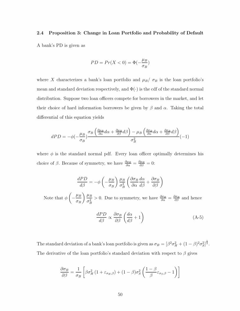
2.4 Proposition 3: Change in Loan Portfolio and Probability of Default

A bank’s PD is given as

PD = Pr(X < 0) = Φ(−µB

σB

)

where X characterizes a bank’s loan portfolio and µB/ σB is the loan portfolio’s

mean and standard deviation respectively, and Φ(·) is the cdf of the standard normal

distribution. Suppose two loan officers compete for borrowers in the market, and let

their choice of hard information borrowers be given by β and α. Taking the total

differential of this equation yields

dPD = −φ(−µB

σB

)σB

(

∂µB

∂αdα + ∂µB

∂βdβ

)

− µB

(

∂σB

∂αdα+ ∂σB

∂βdβ

)

σ2B

(−1)

where φ is the standard normal pdf. Every loan officer optimally determines his

choice of β. Because of symmetry, we have ∂µB

∂α= ∂µB

∂β= 0:

dPD

dβ= −φ

(

−µB

σB

)

µB

σ2B

(

∂σB

∂α

dα

dβ+

∂σB

∂β

)

Note that φ

(

−µB

σB

)

µB

σ2B

> 0. Due to symmetry, we have ∂σB

∂α= ∂σB

∂βand hence

dPD

dβ∝

∂σB

∂β

(

dα

dβ+ 1

)

(A-5)

The standard deviation of a bank’s loan portfolio is given as σB = [β2σ2H + (1− β)2σ2

S]12 .

The derivative of the loan portfolio’s standard deviation with respect to β gives

∂σB

∂β=

1

σB

[

βσ2H (1 + εσH ,β) + (1− β)σ2

S

(

1− β

βεσS ,β − 1

)]

50

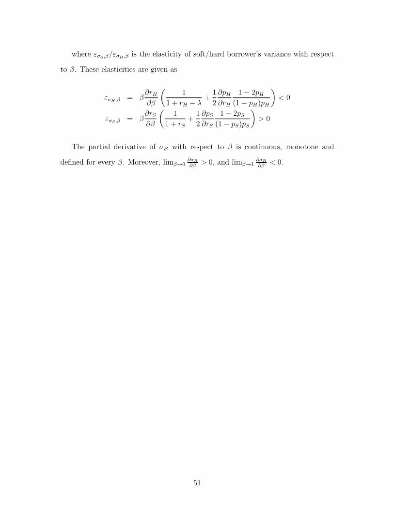
where εσS ,β/εσH ,β is the elasticity of soft/hard borrower’s variance with respect

to β. These elasticities are given as

εσH ,β = β∂rH∂β

(

1

1 + rH − λ+

1

2

∂pH∂rH

1− 2pH(1− pH)pH

)

< 0

εσS ,β = β∂rS∂β

(

1

1 + rS+

1

2

∂pS∂rS

1− 2pS(1− pS)pS

)

> 0

The partial derivative of σB with respect to β is continuous, monotone and

defined for every β. Moreover, limβ→0∂σB

∂β> 0, and limβ→1

∂σB

∂β< 0.

51

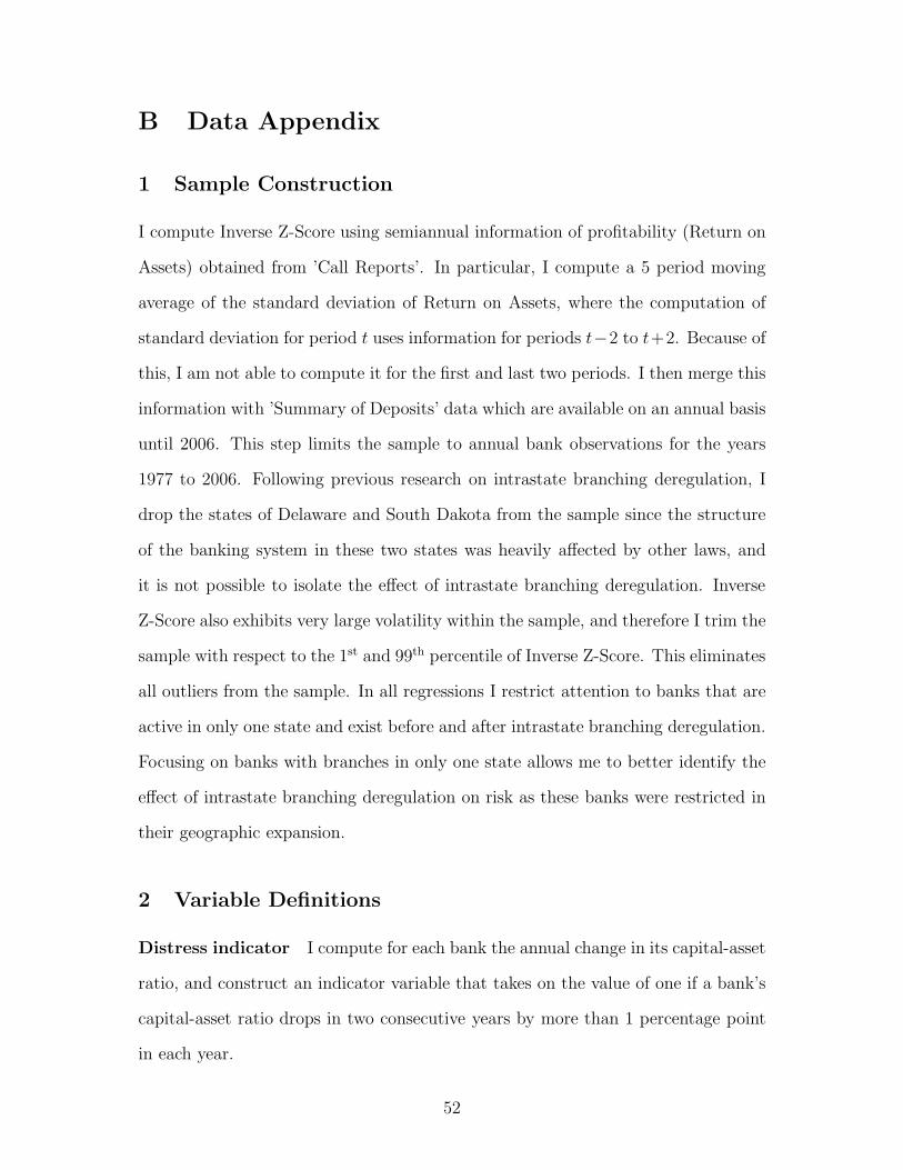
B Data Appendix

1 Sample Construction

I compute Inverse Z-Score using semiannual information of profitability (Return on

Assets) obtained from ’Call Reports’. In particular, I compute a 5 period moving

average of the standard deviation of Return on Assets, where the computation of

standard deviation for period t uses information for periods t−2 to t+2. Because of

this, I am not able to compute it for the first and last two periods. I then merge this

information with ’Summary of Deposits’ data which are available on an annual basis

until 2006. This step limits the sample to annual bank observations for the years

1977 to 2006. Following previous research on intrastate branching deregulation, I

drop the states of Delaware and South Dakota from the sample since the structure

of the banking system in these two states was heavily affected by other laws, and

it is not possible to isolate the effect of intrastate branching deregulation. Inverse

Z-Score also exhibits very large volatility within the sample, and therefore I trim the

sample with respect to the 1st and 99th percentile of Inverse Z-Score. This eliminates

all outliers from the sample. In all regressions I restrict attention to banks that are

active in only one state and exist before and after intrastate branching deregulation.

Focusing on banks with branches in only one state allows me to better identify the

effect of intrastate branching deregulation on risk as these banks were restricted in

their geographic expansion.

2 Variable Definitions

Distress indicator I compute for each bank the annual change in its capital-asset

ratio, and construct an indicator variable that takes on the value of one if a bank’s

capital-asset ratio drops in two consecutive years by more than 1 percentage point

in each year.

52

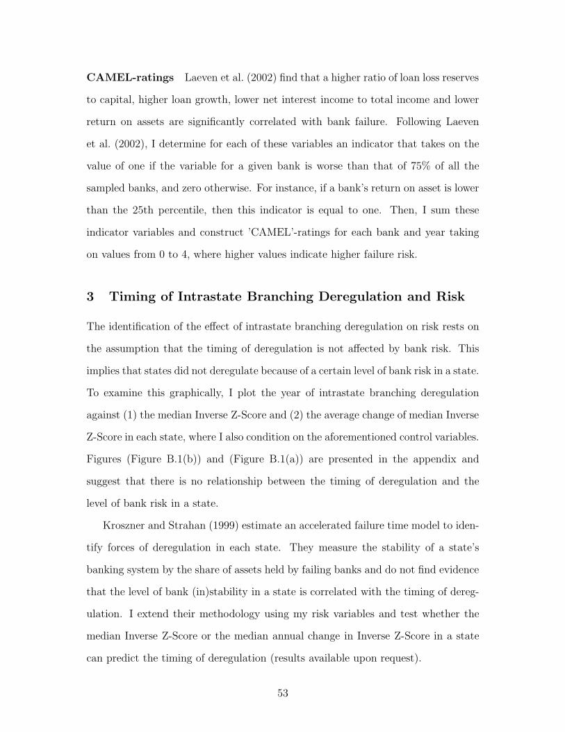
CAMEL-ratings Laeven et al. (2002) find that a higher ratio of loan loss reserves

to capital, higher loan growth, lower net interest income to total income and lower

return on assets are significantly correlated with bank failure. Following Laeven

et al. (2002), I determine for each of these variables an indicator that takes on the

value of one if the variable for a given bank is worse than that of 75% of all the

sampled banks, and zero otherwise. For instance, if a bank’s return on asset is lower

than the 25th percentile, then this indicator is equal to one. Then, I sum these

indicator variables and construct ’CAMEL’-ratings for each bank and year taking

on values from 0 to 4, where higher values indicate higher failure risk.

3 Timing of Intrastate Branching Deregulation and Risk

The identification of the effect of intrastate branching deregulation on risk rests on

the assumption that the timing of deregulation is not affected by bank risk. This

implies that states did not deregulate because of a certain level of bank risk in a state.

To examine this graphically, I plot the year of intrastate branching deregulation

against (1) the median Inverse Z-Score and (2) the average change of median Inverse

Z-Score in each state, where I also condition on the aforementioned control variables.

Figures (Figure B.1(b)) and (Figure B.1(a)) are presented in the appendix and

suggest that there is no relationship between the timing of deregulation and the

level of bank risk in a state.

Kroszner and Strahan (1999) estimate an accelerated failure time model to iden-

tify forces of deregulation in each state. They measure the stability of a state’s

banking system by the share of assets held by failing banks and do not find evidence

that the level of bank (in)stability in a state is correlated with the timing of dereg-

ulation. I extend their methodology using my risk variables and test whether the

median Inverse Z-Score or the median annual change in Inverse Z-Score in a state

can predict the timing of deregulation (results available upon request).

53

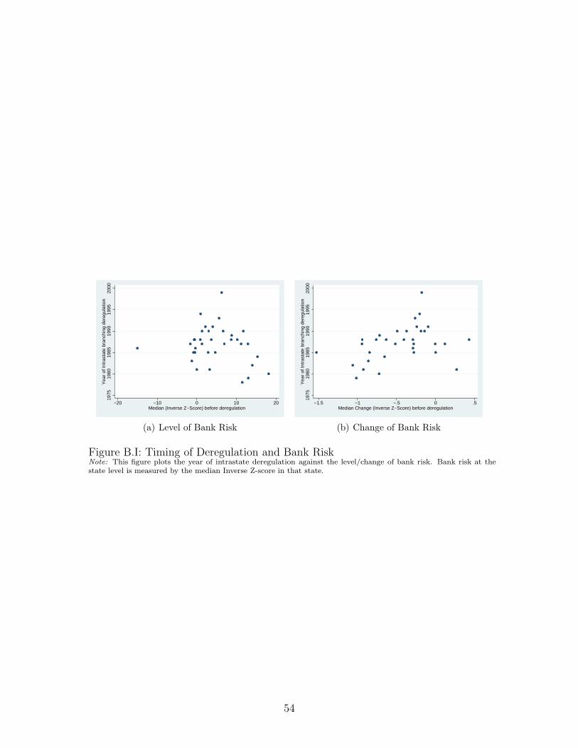
1975

1980

1985

1990

1995

2000

Yea

r of

Intr

asta

te b

ranc

hing

der

egul

atio

n

−20 −10 0 10 20Median (Inverse Z−Score) before deregulation

(a) Level of Bank Risk

1975

1980

1985

1990

1995

2000

Yea

r of

Intr

asta

te b

ranc

hing

der

egul

atio

n

−1.5 −1 −.5 0 .5Median Change (Inverse Z−Score) before deregulation

(b) Change of Bank Risk

Figure B.I: Timing of Deregulation and Bank RiskNote: This figure plots the year of intrastate deregulation against the level/change of bank risk. Bank risk at thestate level is measured by the median Inverse Z-score in that state.

54

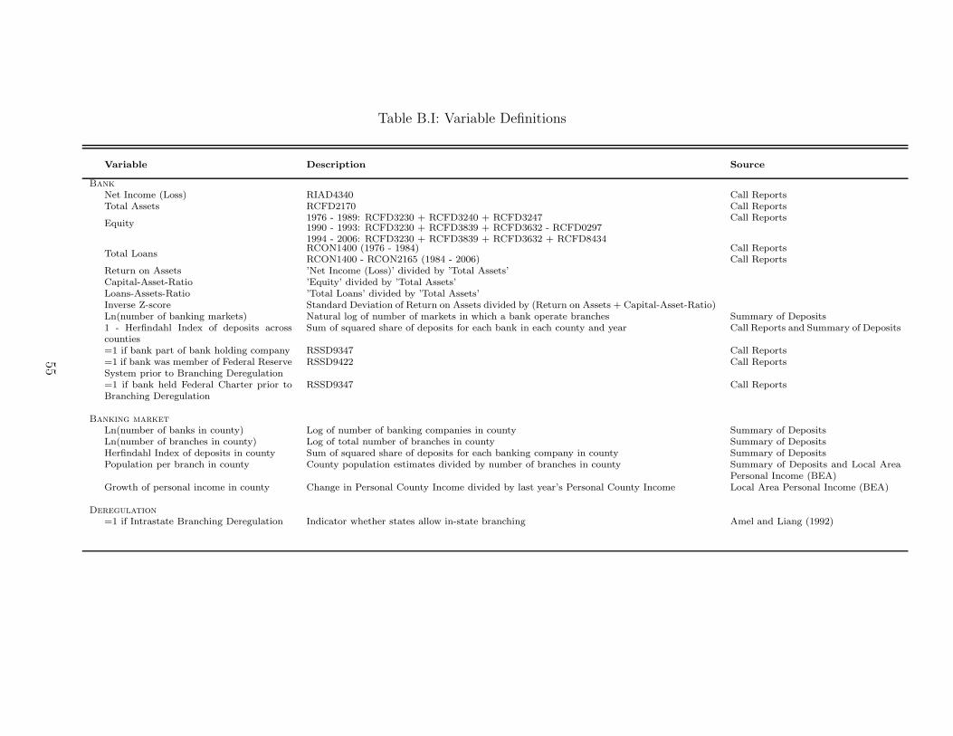
Table B.I: Variable Definitions

Variable Description Source

Bank

Net Income (Loss) RIAD4340 Call ReportsTotal Assets RCFD2170 Call Reports

Equity1976 - 1989: RCFD3230 + RCFD3240 + RCFD3247 Call Reports1990 - 1993: RCFD3230 + RCFD3839 + RCFD3632 - RCFD02971994 - 2006: RCFD3230 + RCFD3839 + RCFD3632 + RCFD8434

Total LoansRCON1400 (1976 - 1984) Call ReportsRCON1400 - RCON2165 (1984 - 2006) Call Reports

Return on Assets ’Net Income (Loss)’ divided by ’Total Assets’Capital-Asset-Ratio ’Equity’ divided by ’Total Assets’Loans-Assets-Ratio ’Total Loans’ divided by ’Total Assets’Inverse Z-score Standard Deviation of Return on Assets divided by (Return on Assets + Capital-Asset-Ratio)Ln(number of banking markets) Natural log of number of markets in which a bank operate branches Summary of Deposits1 - Herfindahl Index of deposits acrosscounties

Sum of squared share of deposits for each bank in each county and year Call Reports and Summary of Deposits

=1 if bank part of bank holding company RSSD9347 Call Reports=1 if bank was member of Federal ReserveSystem prior to Branching Deregulation

RSSD9422 Call Reports

=1 if bank held Federal Charter prior toBranching Deregulation

RSSD9347 Call Reports

Banking market

Ln(number of banks in county) Log of number of banking companies in county Summary of DepositsLn(number of branches in county) Log of total number of branches in county Summary of DepositsHerfindahl Index of deposits in county Sum of squared share of deposits for each banking company in county Summary of DepositsPopulation per branch in county County population estimates divided by number of branches in county Summary of Deposits and Local Area

Personal Income (BEA)Growth of personal income in county Change in Personal County Income divided by last year’s Personal County Income Local Area Personal Income (BEA)

Deregulation

=1 if Intrastate Branching Deregulation Indicator whether states allow in-state branching Amel and Liang (1992)

55

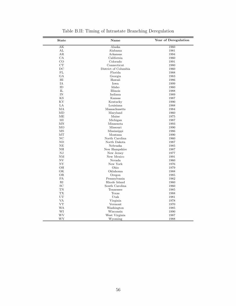
Table B.II: Timing of Intrastate Branching Deregulation

State Name Year of Deregulation

AK Alaska 1960AL Alabama 1981AR Arkansas 1994CA California 1960CO Colorado 1991CT Connecticut 1980DC District of Columbia 1960FL Florida 1988GA Georgia 1983HI Hawaii 1986IA Iowa 1999ID Idaho 1960IL Illinois 1988IN Indiana 1989KS Kansas 1987KY Kentucky 1990LA Louisiana 1988MA Massachusetts 1984MD Maryland 1960ME Maine 1975MI Michigan 1987MN Minnesota 1993MO Missouri 1990MS Mississippi 1986MT Montana 1990NC North Carolina 1960ND North Dakota 1987NE Nebraska 1985NH New Hampshire 1987NJ New Jersey 1977NM New Mexico 1991NV Nevada 1960NY New York 1976OH Ohio 1979OK Oklahoma 1988OR Oregon 1985PA Pennsylvania 1982RI Rhode Island 1960SC South Carolina 1960TN Tennessee 1985TX Texas 1988UT Utah 1981VA Virginia 1978VT Vermont 1970WA Washington 1985WI Wisconsin 1990WV West Virginia 1987WY Wyoming 1988

56