Bargaining and Network Structure: An Experiment^

Gary Charness, Margarida Corominas-Bosch & Guillaume R. Frechette*

October 23, 2003

Abstract: We consider bargaining in a bipartite network of buyers and sellers, who can onlytrade with the limited number of people with whom they are connected. Such networks couldarise due to proximity issues or restricted communication flows, as with informationtransmission of job openings, business opportunities, and transactions not easily regulated byexternal authorities. We perform an experimental test of a graph-theoretic model that allows usto decompose any two-sided network into simple networks of three types, with uniquepredictions about equilibrium prices for the networks in our sessions. We begin with twoseparate simple networks, which are then joined by an additional link. Participants appear toquickly grasp important characteristics of the networks. The results diverge sharply dependingon how this connection is made, typically conforming to the theoretical directional predictions.Payoffs can be systematically affected even for agents who are not connected by the new link.We find evidence of a form of social learning – the shares (publicly) allocated to others in thepast affect what one is willing to accept.

Keywords: Bargaining, Experiment, Graph Theory, Network, Social Learning

JEL Classification: C70, C78, C91, D40

^We would like to thank Jim Andreoni, Ted Bergstrom, Antonio Cabrales, Antoni Bosch, Antoni Calvó-Armengol,Tim Cason, Rachel Croson, Vince Crawford, Martin Dufwenberg, Drew Fudenberg, Uri Gneezy, Brit Grosskopf,Esther Hauk, Robin Hogarth, Matt Jackson, Linda Karr, Tom Palfrey, Larry Samuelson, George Wu, participants ina pilot session at Universitat Pompeu Fabra, and seminar participants at Universitat Pompeu Fabra, UC – Berkeley,the 2001 ESA meetings in Tucson, the 2001 SEA meetings in Tampa, the 2002 Southwest Theory Conference atUCSD, the Graduate School of Business of the University of Chicago, Purdue University, the University ofWisconsin, and UCSB for their valuable comments. The usual disclaimer applies.* Contact: Gary Charness, Dept. of Economics, UCSB, Santa Barbara, CA, 93106-9210, charness@econ.ucsb.edu;Margarida Corominas-Bosch, Dept. of Economics and Business, Universitat Pompeu Fabra, Barcelona, Spain,mcorominasb@campus.uoc.es, Guillaume R. Frechette, Harvard Business School, Boston, MA,gfrechette@hbs.edu. We gratefully acknowledge experimental funds from Spain’s Ministry of Education undergrants PB98-1076 and DI000216. Charness also gratefully acknowledges support from the MacArthur Foundation.This research was undertaken while Charness was affiliated with Universitat Pompeu Fabra.

1

In institutions such as financial markets, people make independent and anonymous

decisions that interact through a central clearing mechanism that matches buyer and seller.1

However, in other environments, individual agents are only in contact with a small number of

other agents, and transactions can only take place if there is a direct ‘link’ (e.g., a social or

business relationship) connecting two agents. In this sense one can talk about a network, which

summarizes the structure of linkages among people. Intuitively, some connections may be better

than others.

Network structure has economic implications for a wide range of situations that feature a

limited number of agents and connections. A market may be inherently thin, as with exclusive

dealers, airplane or arms sales, or international relations. Even where there are many players,

useful information may be transmitted only through private channels, as is often the case for job

openings, business opportunities, and confidential transactions. A network is a non-market

institution, with important market-like characteristics. It can be seen to represent an intermediate

case between bilateral bargaining and matching in a large centralized market.2

Social networks may play an important role where there is little effective external

regulation. For example, Lamoureaux (1986, p. 648) states that “the operation of New England

banks [in the first half of the nineteenth century] was shaped primarily by kinship networks,” and

attributes the successful industrialization of the region to these networks. Guseva and Rona-Tas

(2001) find that social and business networks ameliorated problems in the emerging Russian

1 Nevertheless, there are still human agents in this system. Professional traders and market makers may stronglyprefer to transact with others of their cohort, so that links may still play a role.2 Roth, Prasnikar, Okuno-Fujiwara & Zamir (1991) highlight the effect of competition, demonstrating that resultsare very different for an ultimatum game, with one-to-one matching, and a ‘market game’, where a single agent onone side can agree to a proposal from any of nine agents on the other side.

2

credit-card market in the early 1990s, which suffered from both difficulties in screening

applicants and a lack of effective punishment or sanctions for violations.

While theoretical work on network structure has been progressing rapidly, there have

been few empirical tests; however, the stylized theoretical environment lends itself to laboratory

experiments. In this paper, we assume that the basic network structure is exogenously given.

While this is clearly not the case in many environments, here the imposed network structure

could be seen as representing social, legal, or cultural trading restrictions. This abstraction

allows us to focus on the issue of the resulting bargaining allocations once the network has

reached the form we consider. We extend the infinite-horizon Corominas-Bosch (forthcoming)

graph-theoretic model of buyers and sellers to a finite-horizon experimental game. The model

allows us to decompose any countable number of agents into relatively simple subgraphs (plus

some extra links), with unique payoffs for each buyer and seller, so that our results may therefore

also be applied to larger bipartite networks.

This decomposition determines whether any particular link is relevant to the local

equilibrium price. The process of price formation is central in economics, and there are many

applications for which the traditional Walrasian approach seems inadequate. Rubinstein and

Wolinsky (1985), Gale (1987), and others model price formation as an outcome of decentralized

bilateral bargaining. Pairs of traders who reach agreements leave the market, and those

remaining (and re-matched) continue to bargain, as in our design.

We perform a test on whether it matters how a simple link is added between two small

groups of traders. One link is theoretically irrelevant, while the other should have dramatic

effects. We find that the manner in which the link is added has a major impact on the

bargaining outcome, as the results diverge sharply across treatments and broadly conform to the

3

theoretical predictions. Payoffs can be systematically affected even for agents who are not

connected by the new link.

Most of the discrepancies between the data and theoretical predictions seem to be

attributable to two behavioral phenomena: First, we find that people receive significantly less

when they have only one connection, even where the theory predicts no difference in outcomes.

Perhaps having only a single connection makes one nervous, or inspires perceived bargaining

weakness. Second, we see strong evidence of social learning (Ellison and Fudenberg 1993)

taking place, as the shares (publicly) allocated to others in the past substantially and significantly

affect what one is willing to accept. Given that social learning is concerned with the choices and

outcomes of one’s neighbors, experimental networks would seem to be a promising avenue for

gathering empirical data.

1. Background

In economics, network analysis has been applied to systems compatibility (Katz and

Shapiro 1994), airline route design (Hendricks, Piccione & Tan 1995), matching markets (Gale

and Shapley 1962, Kelso and Crawford 1982, Roth 1984, Crawford and Rochford 1986, Roth

and Sotomayor 1989), and bargaining (Kranton and Minehart 2001). Network structure also

plays a critical role in the optimization of communication and transportation grids.3 Job search

and labor market issues seem particularly suitable for network analysis, since workers frequently

find jobs through personal contacts. Boorman (1975) models the structure of social relationships

3 In the organizational behavior literature, Bolton, Chatterjee & Valley (2001) investigate how communication linksaffect coalition negotiations, finding that the available links strongly influence which coalition forms, and howpayoffs within a coalition are distributed. Valley and Thompson (1998) study the effect of ‘sticky ties’ onorganizational change, suggesting that after a significant organizational change, individuals still prefer to interactwith those other individuals with whom they have ties but no ongoing task relationship, and only change thisbehavior rather slowly. Camerer and Weber (2001) study organizational culture and productivity, highlighting

4

as a graph with undirected ties connecting individuals. Montgomery (1991) studies the effect of

social networks on labor-market outcomes. Calvó-Armengol (2001a) establishes a relationship

between the social structure of bilateral contacts and the job-search process.

A number of field environments loosely fit the type of interaction that we study in our

experiment. For example, consider environments in which products are so expensive that very

few companies can produce them, and only a few entities can make a purchase. Cases in point

are planes produced by Boeing and Airbus, or locomotives and wagons for subway systems

produced by a few companies such as Bonbardier and bought by a very limited number of

metropolitan agencies. While most buyers are connected with most sellers in these examples,

connections are sparser for markets in arms or cigars. For instance, in the latter case, the few

major distributors in Canada are connected to the producers in Cuba and a few other countries

such as Nicaragua, whereas American distributors are not connected to Cuba.4

There are two strands to the network literature in economics. One branch of research

examines the process of network formation. Jackson and Wolinsky (1996) define and discuss

the equilibrium concept of pairwise stability, and use cooperative game theory to examine issues

such as network formation, and consider which networks fulfill stability or efficiency properties.5

Jackson and Watts (forthcoming) and Bala and Goyal (2000) also address the dynamics of non-

cooperative network formation. Kranton and Minehart (2001) study why bilateral networks arise

and whether they are efficient, concluding that networks can enable agents to pool uncertainty in

demand and that efficient networks are an equilibrium of their network formation game.

cultural conflict and merger failure. They find that cultural differences can lead to problems in integrating mergedfirms and that subjects are unaware of the extent to which culture can create integration problems.4 Perhaps more importantly, these examples are probably best thought of as a simultaneous (rather than a sequential)bargaining game, which will be seen to be an important characteristic of our model.5 The network in Corominas-Bosch (forthcoming) can be considered to represent an assignment game in the sense ofShapley and Shubik (1972), where buyers value the goods of sellers at either 0 (if they are not connected) or 1 (if

5

The second strand considers the impact of exogenously-specified network structures on

outcomes. Bala and Goyal (1998) model social learning, Glaeser, Sacerdote & Sheinkman

(1996) study applications to crime patterns in urban areas, and Morris (2000) examines social

coordination. Chwe (2000) shows that ‘low-dimensional’ networks can be better for

coordination, even though they have fewer links than ‘high-dimensional’ networks. Calvó-

Armengol (2001b) derives a measure of bargaining power in n-player networks, using a form of

sequential bargaining.

Our study relates to the second strand, as we do not consider the issue of how networks

were formed, or which networks we might expect to form if there are modest costs to forming (or

severing) links. Our motivation for considering exogenously-specified networks is that we are

primarily interested in isolating the effect of a small change in network structure on bargaining

behavior and prices. We simply presume that the links are already in place due to some

relationships that have (or had) value, and that the cost of (endogenous) change is prohibitive. In

this sense, the networks we use are effectively stable and have immediate economic application.

There are now several network experiments in economics; for an excellent survey of this

embryonic field, see Kosfeld (2003). Corbae and Duffy (2001) study 2x2 games, where

participants play all of their ‘neighbors’ in the network. Cassar (2002) finds that play in a

coordination game typically converges to the efficient Nash equilibrium in a ‘small-world’

network, but does so less frequently with local interaction or a random network. Deck and

Johnson (2002) examine the effect of cost-sharing institutions in endogenous networks, obtaining

slightly better efficiency when players can bid between zero and the full cost of a direct link.

Riedl and Ule (2002) consider partner-selection in a prisoner’s dilemma, finding stable

they are connected). When our experimental setup is transformed into a cooperative game, we note that the uniquePEP of the networks analyzed lies in the core of the assignment game. See Corominas-Bosch (1999) for details.

6

cooperation when people can choose their own partners. Falk and Kosfeld (2003) find that the

Bala and Goyal (2000) model predicts outcomes fairly well with one-way flows, but does quite

poorly with two-way flows.6 While all of these studies consider network-related issues, none

directly address the asymmetrical nature of many networks, how network structure affects

bargaining outcomes, or the value of different links.

The largest literature on networks can be found in sociology, where the focus is on the

exercise of power.7 Instead of having better skills, a person may be somehow better connected,

so that social capital is the contextual complement to human capital. Stolte and Emerson (1977)

and Cook and Emerson (1978) were the first to conduct experimental research on network

structure. Lovaglia, Skvoretz, Willer, and Markovsky (1995) and Willer, Lovaglia, and

Markovsky (1997) use network exchange theory (Markovsky, Willer, and Patton 1988) and a

‘power index’ to predict power (which relates to exclusion from exchange) and profit rankings in

social exchange networks.8 The sociology experiments clearly demonstrate that power can flow

through the links in a network. However, the designs employed are not really suited to tests of

non-cooperative bargaining theory for two-sided markets with multiple agents on each side.

The social-learning literature generally considers the effect of dynamic aggregation of

social information on equilibrium outcomes. Ellison and Fudenberg (1993, p. 612) use the term

social learning to describe contexts where “agents base their decisions, at least in part, on the

experience of their neighbors,” listing (p. 613) three features for such learning environments, all

6 Kirchkamp and Nagel (forthcoming) study a prisoner’s dilemma game with local interaction. Berninghaus Ehrhart& Keser,(1998) use a 3-person game; participants are either connected to neighbors on a circle or play within closedthree-person groups.7 See Willer (1999) and Burt (2000) for discussions of the literature and issues in this field.8 In a similar spirit, the Calvó-Armengol (2001b) formal model uses a measure in which one’s bargaining powerincreases as the number of people one’s neighbors can reach decreases.

7

of which are satisfied here.9 Ellison and Fudenberg (1995) find that word-of-mouth

communication may lead to superior choices and socially-efficient outcomes. Jackson and Kalai

(1997) study recurring games, where a stage game is played repeatedly, but each stage is played

by a new group of players. This set-up seems closest in spirit to our game, but involves signals

that shed light on the distribution of types in the population.10

2. The Model

Corominas-Bosch (forthcoming) provides a method for decomposing a network of buyers

and sellers into relatively simple subgraphs, plus some extra links. Our adaption to the

laboratory is a two-sided market, with two types of agents (e.g., buyers and sellers) who engage

in sequential bargaining – alternating offers over a shrinking pie, with multiple possible rounds.

Suppose there are n sellers and m buyers of a homogenous good for which all sellers have

reservation value 0 and all buyers have reservation value 1. Each buyer desires only one unit of

the good, and each seller can supply only one unit. Is the price dependent only on the relative

sizes of n and m, and will all trades take place at the same price? Here buyers (sellers) bargain

with a pre-assigned subset of all sellers (buyers); links are non-directed, which means that A is

linked to B if and only if B is linked to A. Any buyer may be connected to multiple sellers and

vice versa. The network structure is common information, as are all proposals and

acceptances.11

Our analysis incorporates the following intuition: Some networks are ‘competitive’, so

that the short side of the market receives all surplus. On the other hand, other networks are

9 1) Agents observe both their neighbors’ choices and the payoffs that these choices generate; 2) Agents periodicallyreevaluate their decisions, as opposed to making a once-and-for-all choice; 3) Players may be sufficientlyheterogeneous that under full information they would not all make the same choice. In our case, one’s neighbors arein a sense temporal.10 See also Jackson and Kalai (1999) and Bala and Goyal (1998, 2001).

8

‘even’ (neither of the sides is stronger), and agents split the payoffs nearly evenly. This structure

generalizes to any network, and we can decompose any network into a union of smaller

networks, each one either a competitive or an even network, plus some extra links.

Consider three types of particular bipartite graphs (GS, GE, and GB). Let graphs GS be

those with more sellers than buyers, such that any set of sellers can be ‘jointly matched’ with

buyers if the number of sellers in this set does not exceed the number of buyers.12 In the

following figure, G1 is of type GS since it has more sellers than buyers (3 versus 2), and since we

can find a joint matching involving any set of 1 or 2 sellers. Graphs GB are the complement,

substituting sellers for buyers and vice versa. Finally, graphs GE have as many sellers and

buyers and are such that there exists a joint matching involving all of them.

G3 : type GBG1 : type GS G2 : type GE

Not every graph is one of these three types, as is illustrated by the following graph:

Nevertheless, we can decompose this graph into two subgraphs, one of type GS and one

of type GE, plus an extra link.

11 Of course, bargainers maintain personal anonymity in the laboratory.12 Intuitively, a set of sellers can be jointly matched if there exists a collection of pairs of linked members such thateach agent belongs to at most one pair. See Appendix A for more detail and the formal definitions.

9

GS GE

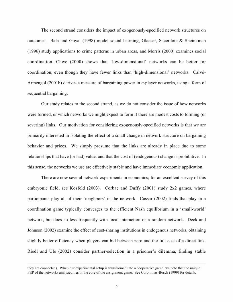
Theorem 1 (shown in Appendix A) shows that any graph decomposes as a union of

subgraphs which are of one of these three types, plus some extra links which will never connect a

buyer in a subgraph GB with a seller in a subgraph GS. As in Corominas-Bosch (forthcoming), a

simple iterative algorithm for decomposing countable bipartite networks is at the heart of the

process.13

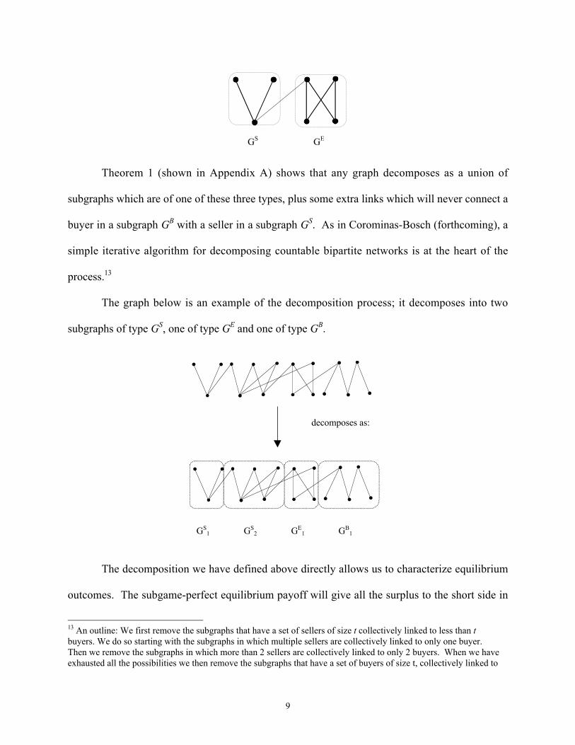
The graph below is an example of the decomposition process; it decomposes into two

subgraphs of type GS, one of type GE and one of type GB.

decomposes as:

GS1 GS

2 GE1 GB

1

The decomposition we have defined above directly allows us to characterize equilibrium

outcomes. The subgame-perfect equilibrium payoff will give all the surplus to the short side in

13 An outline: We first remove the subgraphs that have a set of sellers of size t collectively linked to less than tbuyers. We do so starting with the subgraphs in which multiple sellers are collectively linked to only one buyer.Then we remove the subgraphs in which more than 2 sellers are collectively linked to only 2 buyers. When we haveexhausted all the possibilities we then remove the subgraphs that have a set of buyers of size t, collectively linked to

10

the subgraphs that are GS or GB (competitive networks), while the surplus will be split relatively

evenly (taking into account the first mover advantage) in GE subgraphs (even networks). We

demonstrate below precisely how this works for the particular networks and procedures used in

our experimental design.

Implementation

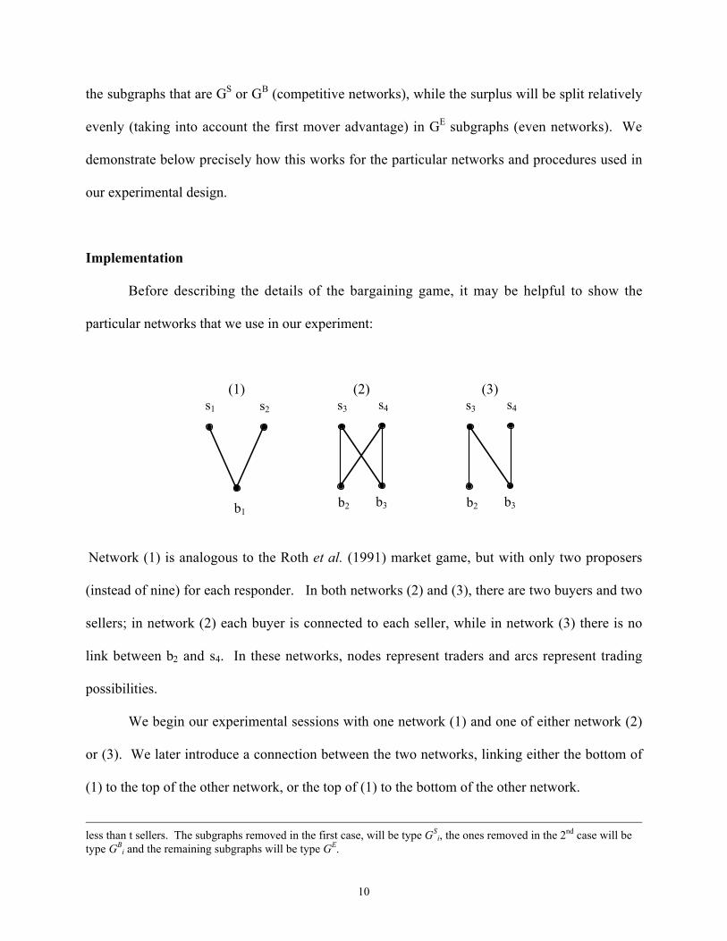
Before describing the details of the bargaining game, it may be helpful to show the

particular networks that we use in our experiment:

(1) (2) (3) s1

b1

s2 s3 s4

b2 b3

s3 s4

b2 b3

Network (1) is analogous to the Roth et al. (1991) market game, but with only two proposers

(instead of nine) for each responder. In both networks (2) and (3), there are two buyers and two

sellers; in network (2) each buyer is connected to each seller, while in network (3) there is no

link between b2 and s4. In these networks, nodes represent traders and arcs represent trading

possibilities.

We begin our experimental sessions with one network (1) and one of either network (2)

or (3). We later introduce a connection between the two networks, linking either the bottom of

(1) to the top of the other network, or the top of (1) to the bottom of the other network.

less than t sellers. The subgraphs removed in the first case, will be type GS

i, the ones removed in the 2nd case will betype GB

i and the remaining subgraphs will be type GE.

11

In the first round of bargaining, sellers simultaneously make proposals to divide 2500

with any of their linked buyers. These offers are displayed, and buyers then simultaneously

choose to accept at most one of the proposals made by linked sellers. If one or more responders

accept the same share proposed by one or more proposers, players are matched randomly

choosing among all matching schemes that maximize the number of trades.14 This means that

responders actually accept a proposal, but they do not care with which specific proposer they

trade. If a buyer and seller trade, they and their links are removed from the network. If any

linked buyers and sellers remain, the game proceeds to the 2nd round, where buyers now propose

divisions of 2400 to all of their linked sellers, who choose whether to accept. If a 3rd round is

necessary, sellers propose divisions of 2300, etc. There are at most 6 rounds of bargaining; a

coin is flipped in front of the group after round 4 to determine whether the period ends after

round 5 or round 6.15 All unmatched players receive 200.16

Let us examine how to determine the subgame-perfect equilibrium payoffs (subsequently

denoted by PEP). Our analysis begins with the study of the simplest possible cases: Networks

with at most 2 sellers and 2 buyers. We start by considering triads:

14 This assumption is important as it drives the results toward efficiency. Suppose for instance that in network (2)both proposers propose (p, 1-p), and both responders accept the proposal from the same proposer. If agents were tobe forced to choose the proposal and the responder, only one pair would form, even if potentially one couldconstruct two pairs. With the assumption we introduce, both agents will be matched, randomly choosing the exactproposer-responder pairs.15 We introduced this uncertainty in order to prevent unraveling effects, at least prior to round 5.16 We chose a non-zero reservation payoff to avoid having to give individual participants no money other than theshow-up fee. While this may serve to minimize the obvious fairness considerations, we shall see that the passage oftime seems to reduce their impact in any case.

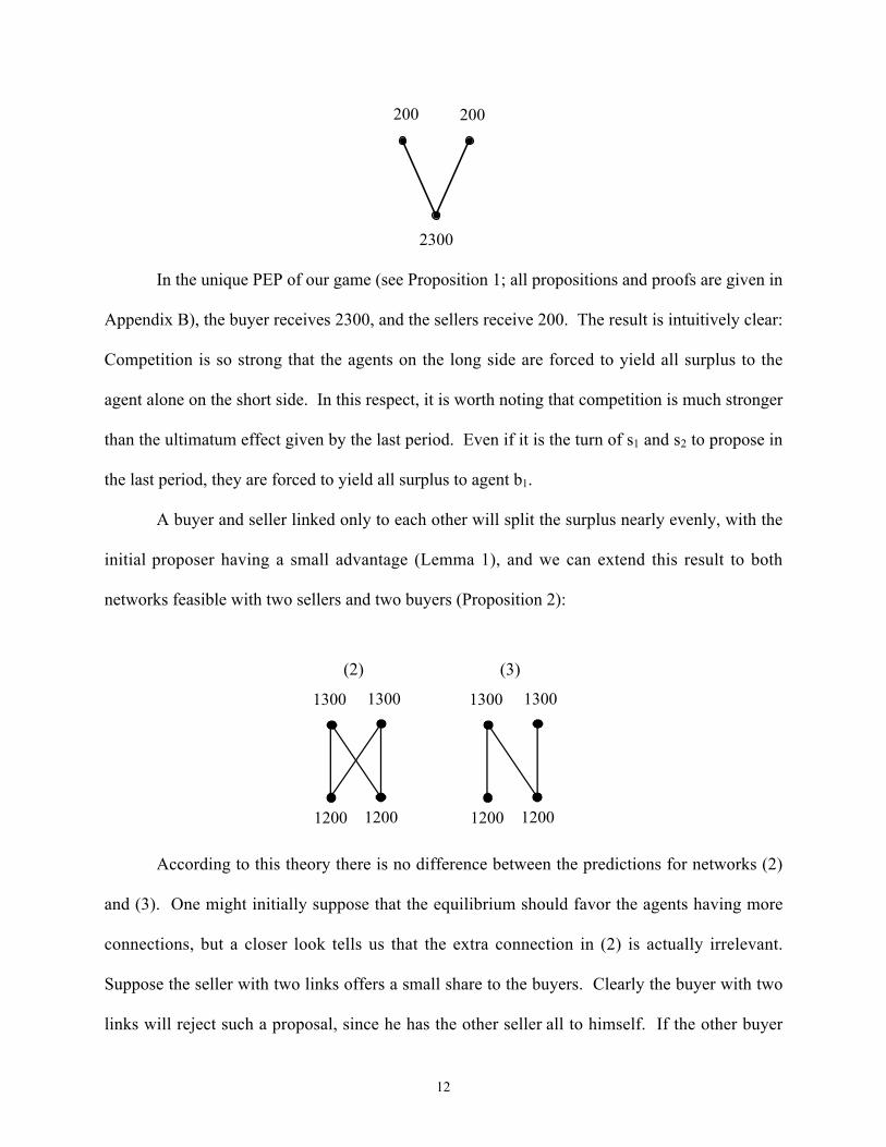
12

200

2300

200

In the unique PEP of our game (see Proposition 1; all propositions and proofs are given in

Appendix B), the buyer receives 2300, and the sellers receive 200. The result is intuitively clear:

Competition is so strong that the agents on the long side are forced to yield all surplus to the

agent alone on the short side. In this respect, it is worth noting that competition is much stronger

than the ultimatum effect given by the last period. Even if it is the turn of s1 and s2 to propose in

the last period, they are forced to yield all surplus to agent b1.

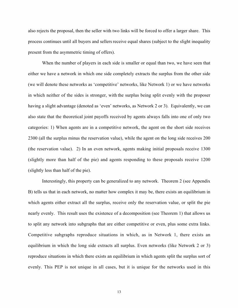
A buyer and seller linked only to each other will split the surplus nearly evenly, with the

initial proposer having a small advantage (Lemma 1), and we can extend this result to both

networks feasible with two sellers and two buyers (Proposition 2):

(2) (3)

1300 1300

1200 1200

1300 1300

1200 1200

According to this theory there is no difference between the predictions for networks (2)

and (3). One might initially suppose that the equilibrium should favor the agents having more

connections, but a closer look tells us that the extra connection in (2) is actually irrelevant.

Suppose the seller with two links offers a small share to the buyers. Clearly the buyer with two

links will reject such a proposal, since he has the other seller all to himself. If the other buyer

13

also rejects the proposal, then the seller with two links will be forced to offer a larger share. This

process continues until all buyers and sellers receive equal shares (subject to the slight inequality

present from the asymmetric timing of offers).

When the number of players in each side is smaller or equal than two, we have seen that

either we have a network in which one side completely extracts the surplus from the other side

(we will denote these networks as ‘competitive’ networks, like Network 1) or we have networks

in which neither of the sides is stronger, with the surplus being split evenly with the proposer

having a slight advantage (denoted as ‘even’ networks, as Network 2 or 3). Equivalently, we can

also state that the theoretical joint payoffs received by agents always falls into one of only two

categories: 1) When agents are in a competitive network, the agent on the short side receives

2300 (all the surplus minus the reservation value), while the agent on the long side receives 200

(the reservation value). 2) In an even network, agents making initial proposals receive 1300

(slightly more than half of the pie) and agents responding to these proposals receive 1200

(slightly less than half of the pie).

Interestingly, this property can be generalized to any network. Theorem 2 (see Appendix

B) tells us that in each network, no matter how complex it may be, there exists an equilibrium in

which agents either extract all the surplus, receive only the reservation value, or split the pie

nearly evenly. This result uses the existence of a decomposition (see Theorem 1) that allows us

to split any network into subgraphs that are either competitive or even, plus some extra links.

Competitive subgraphs reproduce situations in which, as in Network 1, there exists an

equilibrium in which the long side extracts all surplus. Even networks (like Network 2 or 3)

reproduce situations in which there exists an equilibrium in which agents split the surplus sort of

evenly. This PEP is not unique in all cases, but it is unique for the networks used in this

14

experiment. Our derivation closely follows Corominas-Bosch (forthcoming), by adapting the

model of the infinite horizon game treated therein to our finite-horizon game.

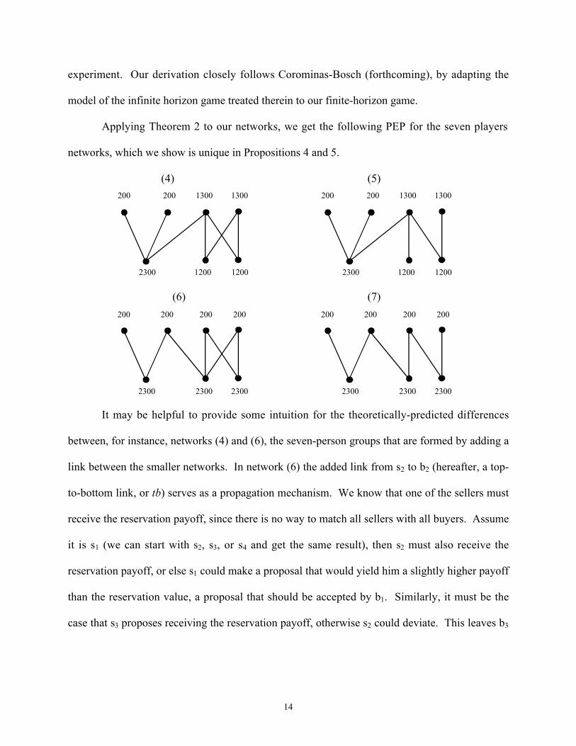
Applying Theorem 2 to our networks, we get the following PEP for the seven players

networks, which we show is unique in Propositions 4 and 5.

(4) (5) 200

2300

200 1300 1300

1200 1200

200

2300

200 1300 1300

1200 1200

(6) (7) 200

2300

200 200 200

2300 2300

200

2300

200 200 200

2300 2300

It may be helpful to provide some intuition for the theoretically-predicted differences

between, for instance, networks (4) and (6), the seven-person groups that are formed by adding a

link between the smaller networks. In network (6) the added link from s2 to b2 (hereafter, a top-

to-bottom link, or tb) serves as a propagation mechanism. We know that one of the sellers must

receive the reservation payoff, since there is no way to match all sellers with all buyers. Assume

it is s1 (we can start with s2, s3, or s4 and get the same result), then s2 must also receive the

reservation payoff, or else s1 could make a proposal that would yield him a slightly higher payoff

than the reservation value, a proposal that should be accepted by b1. Similarly, it must be the

case that s3 proposes receiving the reservation payoff, otherwise s2 could deviate. This leaves b3

15

in a position to also extract surplus. Essentially, the buyers are jointly able to exploit the sellers;

b1, b2, and b3 receive full shares and s1, s2, s3, and s4 receive only the reservation payoffs.

On the other hand, in network (4) there is no propagation across the added link (hereafter,

a bottom-to-top link, or bt). Seller s3 knows that either s1 or s2 must get 0, so that b1 will expect

to get a full share. This implies that s3 eliminates b1 from his bargaining plans, and the (s3,

s4,b2,b3) network can be considered in isolation.

Thus, an apparently minor change in the network (differing by only one connection) may

strongly alter the situation. A new connection can affect players who are not directly involved.

On the other hand, some new connections are theoretically irrelevant.

3. Experimental Design

This experiment was conducted at the Universitat Pompeu Fabra in Barcelona, Spain.

Participants were recruited by posting notices at campus locations. A total of 105 people

participated in our study (each person could only participate in one session). Most of these were

students in economics or business, with a smaller percentage of students in the humanities.

Session lasted about 100 minutes and average earnings were approximately 1600 Spanish

pesetas (at the time, $1 = 140 pesetas), including a show-up fee of 500 pesetas.

Participants were given written instructions (an English translation of the instructions is

presented in Appendix C) and these were read aloud.17 We used a three-person network and one

of two types of four-person networks in the initial phase of our experimental sessions. Thus,

17 The instructions did not correctly reflect the specifications of the theoretical model when two agentssimultaneously accept the same individual’s offer, while there was another identical offer available (see footnote12). However, this situation was rare in the laboratory and was in fact implemented in accordance with our model inthree of the five cases where it occurred.

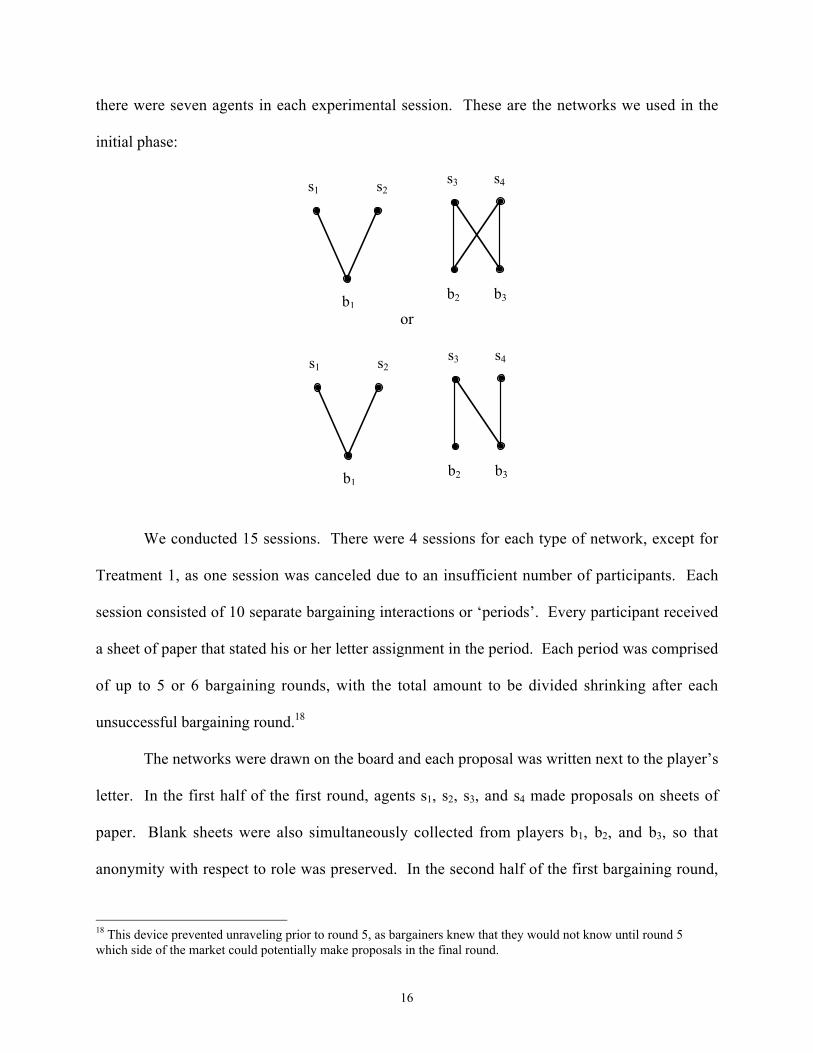
16

there were seven agents in each experimental session. These are the networks we used in the

initial phase:

s2 s1

b1

s3 s4

b2 b3

or

s2 s1

b1

s3 s4

b2 b3

We conducted 15 sessions. There were 4 sessions for each type of network, except for

Treatment 1, as one session was canceled due to an insufficient number of participants. Each

session consisted of 10 separate bargaining interactions or ‘periods’. Every participant received

a sheet of paper that stated his or her letter assignment in the period. Each period was comprised

of up to 5 or 6 bargaining rounds, with the total amount to be divided shrinking after each

unsuccessful bargaining round.18

The networks were drawn on the board and each proposal was written next to the player’s

letter. In the first half of the first round, agents s1, s2, s3, and s4 made proposals on sheets of

paper. Blank sheets were also simultaneously collected from players b1, b2, and b3, so that

anonymity with respect to role was preserved. In the second half of the first bargaining round,

18 This device prevented unraveling prior to round 5, as bargainers knew that they would not know until round 5which side of the market could potentially make proposals in the final round.

17

players b1, b2, and b3 indicated which one (if any) of the outstanding proposals they wished to

accept.19 Acceptances and rejections were indicated on the board and an ellipse was drawn

around links between those agents who had reached agreements, removing them and their links

from the network. Bargaining rounds continued as needed.

The session then proceeded to the next period. Positions were randomly changed in each

period, subject to the constraint that each person remained in their original 3- or 4-person

network.20 We played four periods before adding a link between the two networks and six

periods after the link was added. The number of periods to be played either before or after the

link was added was not divulged to the participants, although they were told that there would be

a change in the network at some point in time. The participants only learned the nature of the

new network at the time that the change was publicly introduced.

People were told that one of the 10 periods would be chosen at random for

implementation of actual monetary payoffs. At the end of the experiment, a 10-sided die was

rolled to determine the period chosen for payment.21 Participants were then paid individually

and privately.

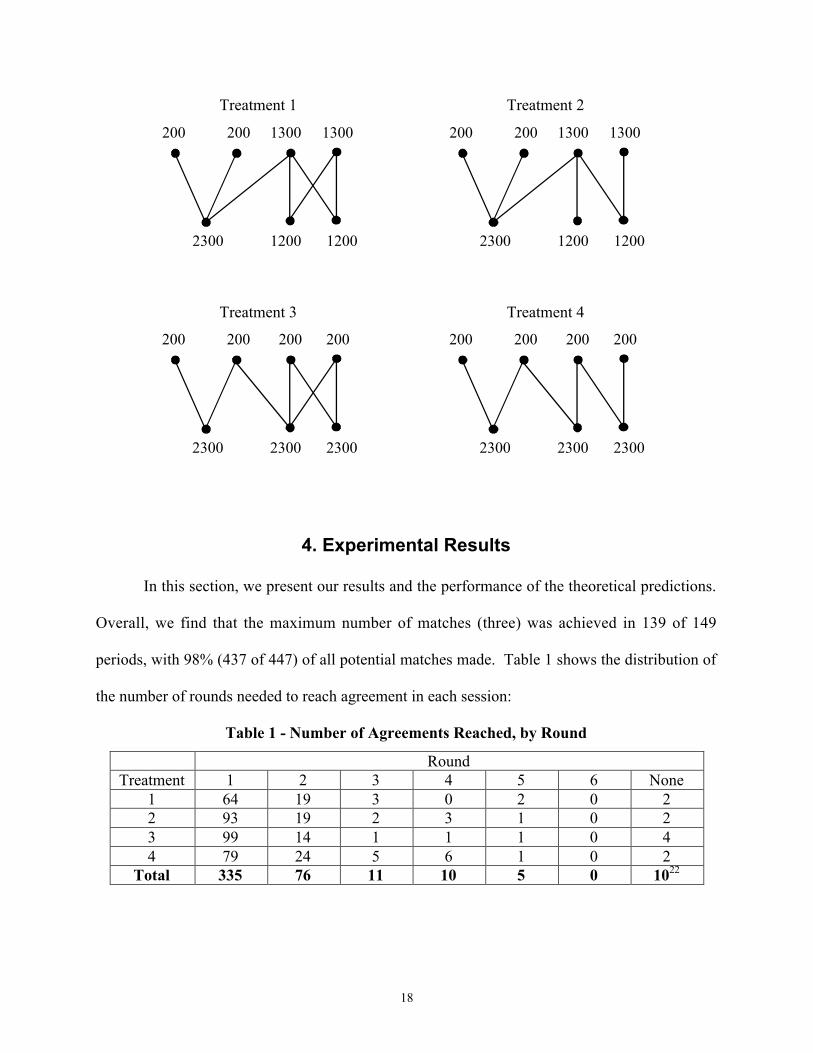
The new link either connected player b1 to player s3 or player s2 to player b2. Applying

Theorem 2, the four possible seven-person networks and the associated unique PEP are:

19 In the 2nd half of the first round, we collected responses from b1, b2, and b3, as well as blank sheets from s1, s2, s3,and s4. In all subsequent rounds (if necessary), we continued to collect sheets from every player.20 It might seem more natural to keep the same letter assignments throughout the session. However, fixed roles inour multi-period design would lead to effective identifiability and repeated-game issues. In addition, role changingallows for ‘smoothing’ of the heterogeneity of individuals and minimizes arbitrary performance by a participantunhappy at being stuck in a disadvantageous role throughout the session.21 This random-payment design avoids possible ‘income effects’ from participants having accumulated wealth inearly periods.

18

Treatment 1 Treatment 2

200

2300

200 1300 1300

1200 1200

200

2300

200 1300 1300

1200 1200

Treatment 3 Treatment 4

200

2300

200 200 200

2300 2300

200

2300

200 200 200

2300 2300

4. Experimental Results

In this section, we present our results and the performance of the theoretical predictions.

Overall, we find that the maximum number of matches (three) was achieved in 139 of 149

periods, with 98% (437 of 447) of all potential matches made. Table 1 shows the distribution of

the number of rounds needed to reach agreement in each session:

Table 1 - Number of Agreements Reached, by Round

RoundTreatment 1 2 3 4 5 6 None

1 64 19 3 0 2 0 22 93 19 2 3 1 0 23 99 14 1 1 1 0 44 79 24 5 6 1 0 2

Total 335 76 11 10 5 0 1022

19

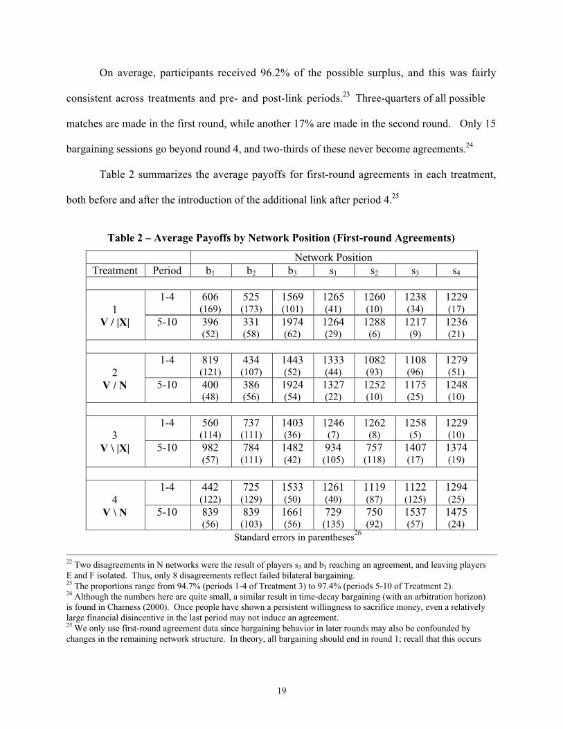
On average, participants received 96.2% of the possible surplus, and this was fairly

consistent across treatments and pre- and post-link periods.23 Three-quarters of all possible

matches are made in the first round, while another 17% are made in the second round. Only 15

bargaining sessions go beyond round 4, and two-thirds of these never become agreements.24

Table 2 summarizes the average payoffs for first-round agreements in each treatment,

both before and after the introduction of the additional link after period 4.25

Table 2 – Average Payoffs by Network Position (First-round Agreements)

Network PositionTreatment Period b1 b2 b3 s1 s2 s3 s4

1-4 606(169)

525(173)

1569(101)

1265(41)

1260(10)

1238(34)

1229(17)1

V / |X| 5-10 396(52)

331(58)

1974(62)

1264(29)

1288(6)

1217(9)

1236(21)

1-4 819(121)

434(107)

1443(52)

1333(44)

1082(93)

1108(96)

1279(51)2

V / N 5-10 400(48)

386(56)

1924(54)

1327(22)

1252(10)

1175(25)

1248(10)

1-4 560(114)

737(111)

1403(36)

1246(7)

1262(8)

1258(5)

1229(10)3

V \ |X| 5-10 982(57)

784(111)

1482(42)

934(105)

757(118)

1407(17)

1374(19)

1-4 442(122)

725(129)

1533(50)

1261(40)

1119(87)

1122(125)

1294(25)4

V \ N 5-10 839(56)

839(103)

1661(56)

729(135)

750(92)

1537(57)

1475(24)

Standard errors in parentheses26

22 Two disagreements in N networks were the result of players s3 and b3 reaching an agreement, and leaving playersE and F isolated. Thus, only 8 disagreements reflect failed bilateral bargaining.23 The proportions range from 94.7% (periods 1-4 of Treatment 3) to 97.4% (periods 5-10 of Treatment 2).24 Although the numbers here are quite small, a similar result in time-decay bargaining (with an arbitration horizon)is found in Charness (2000). Once people have shown a persistent willingness to sacrifice money, even a relativelylarge financial disincentive in the last period may not induce an agreement.25 We only use first-round agreement data since bargaining behavior in later rounds may also be confounded bychanges in the remaining network structure. In theory, all bargaining should end in round 1; recall that this occurs

20

A nonparametric Wilcoxon-Mann-Whitney rank-sum test (Siegel and Castellan 1988) on

payoff changes, using fully-independent session-level data (15 observations), confirms that the

type of link added (tb or bt) strongly affects bargaining behavior. The changes in average (s1,s2)

payoffs and the average difference in (b2,b3) and (s3,s4) payoffs are always highest when a tb link

is added; this reverses for player b1’s payoffs (see Table D1). Each of these comparisons

indicates a difference significant at p = 0.002.

Several implications of the theory can be tested; we first consider the point predictions,

and then discuss the qualitative predictions. Table 3 breaks the average payoff per position

down by link-type, and reports whether the payoff differs (at the 5% significance level) from the

theoretical prediction. We pool all the (first-round agreement) data for s1, b1, and b2, as the type

of link does not affect the predicted payoffs for these positions.27 For s 2, s 3, b 3, and b 4, the

theory distinguishes between whether or not there is a tb link. The columns give the theoretical

predictions, and in each cell the average amount is reported, accompanied by r if the theoretical

prediction is rejected and nr otherwise. As can be seen, only two of the 11 predictions cannot be

rejected. However, the relative magnitudes of the estimates seem to go in the direction

suggested by theory.

75% of the time. This selection criterion will be used in tests throughout the paper, unless otherwise noted. Forcompleteness, the average payoffs for all cases are shown in Appendix D.26 Throughout the paper, whenever standard errors are reported or used in tests, they are adjusted to account for thefact that we have repeated observations for each subject (Cochran 1977, Wolter 1985).27 We note that the apparent differences in A and B payoffs in periods 1-4 in some treatments vanish when these are(appropriately) aggregated across treatments.

21

Table 3 – Tests of the Quantitative Theoretical Predictions

Type Link 200 1200 1300 2300s1 All 641 rs2 All 578 rb1 All 1646 rs3 No tb 1286 nrs3 tb 855 rs4 No tb 1211 rs4 tb 754 rb2 No tb 1188 nrb2 tb 1464 rb3 No tb 1255 rb3 tb 1418 r

To test the qualitative predictions, we first average the payoffs by subject (for each

position and relevant link). Using these per-subject averages, we conduct sign tests. Each cell

compares whether the column and row components are equal, with a one-sided test if there is a

directional hypothesis:

Table 4 – Nonparametric Tests of Payoff Comparisons28

Type s1 s2 s3 s4 b2 b3 s3 s4 b2

Type Link All All No tb No tb No tb No tb tb tb tbs2 All nr, tb1 All r, t r, ts3 No tb rs4 No tb r

nr, t r,t

b2 No tb nr, tb3 No tb

nrnr, t

s4 tb nr, tb2 tbb3 tb

r, t r, tnr, t

r (nr) means we can (cannot) reject (at p = 0.05) the hypothesis that the payoffs are equal.t means the result is consistent with the theory.

All but two of the theoretical predictions find support. Even for the two exceptions, the

difference between actual average payoffs and predicted payoffs is never more than 100.29 We

22

will explore the causes for these deviations in our discussion. Generally the directional

comparisons are very much in line with the theoretical predictions, at high levels of statistical

significance.30

Although the theoretical point predictions generally fail, the evolution of play suggests

that this might be in part remedied over time. The theory seems to fare poorly when it predicts a

very uneven split. In most of these cases however, payoffs either stabilize or move closer and

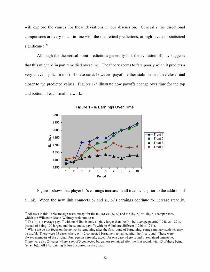
closer to the predicted values. Figures 1-3 illustrate how payoffs change over time for the top

and bottom of each small network.

Figure 1 - b1 Earnings Over Time

1250

1400

1550

1700

1850

2000

2150

2300

1 2 3 4 5 6 7 8 9 10

Period

Ear

ning

s Treat 1Treat 2Treat 3Treat 4

Figure 1 shows that player b1’s earnings increase in all treatments prior to the addition of

a link. When the new link connects b1 and s3, b1’s earnings continue to increase steadily.

28 All tests in this Table are sign tests, except for the (s3, s4) vs. (s3, s4) and the (b2, b3) vs. (b2, b3) comparisons,which are Wilcoxon-Mann-Whitney rank-sum tests.29 The (s3, s4) average payoff with no tb link is only slightly larger than the (b2, b3) average payoff, (1248 vs. 1221),instead of being 100 larger, and the s3 and s4 payoffs with no tb link are different (1286 to 1211).30 While we do not focus on the networks remaining after the first round of bargaining, some summary statistics maybe useful. There were 65 cases where only 2 connected bargainers remained after the first round. These werealways members of the original four-person network, except for one case where s1 and b1 remained unmatched.There were also 24 cases where a set of 3 connected bargainers remained after the first round, with 15 of these being(s3, s2, b1). All 8 bargaining failures occurred in the dyads.

23

However, when the new link connects s2 and b2, b1’s earnings do not change as much after

period 4.

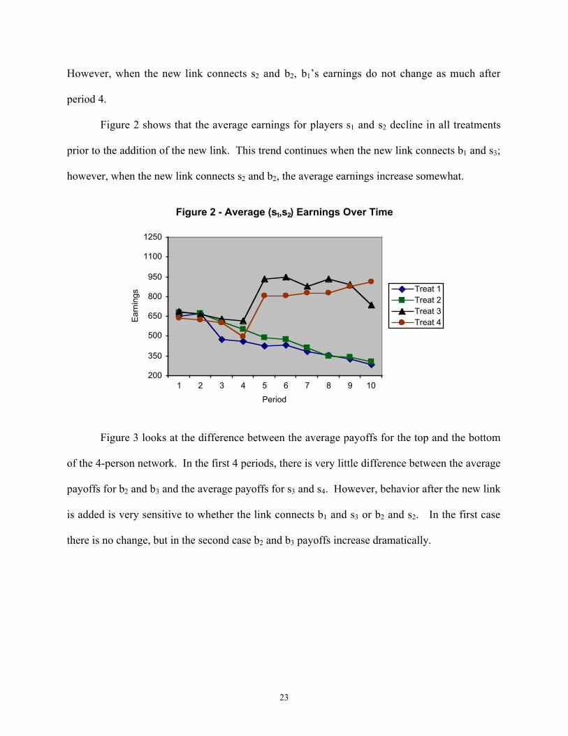
Figure 2 shows that the average earnings for players s1 and s2 decline in all treatments

prior to the addition of the new link. This trend continues when the new link connects b1 and s3;

however, when the new link connects s2 and b2, the average earnings increase somewhat.

Figure 2 - Average (s1,s2) Earnings Over Time

200

350

500

650

800

950

1100

1250

1 2 3 4 5 6 7 8 9 10

Period

Ear

ning

s Treat 1Treat 2Treat 3Treat 4

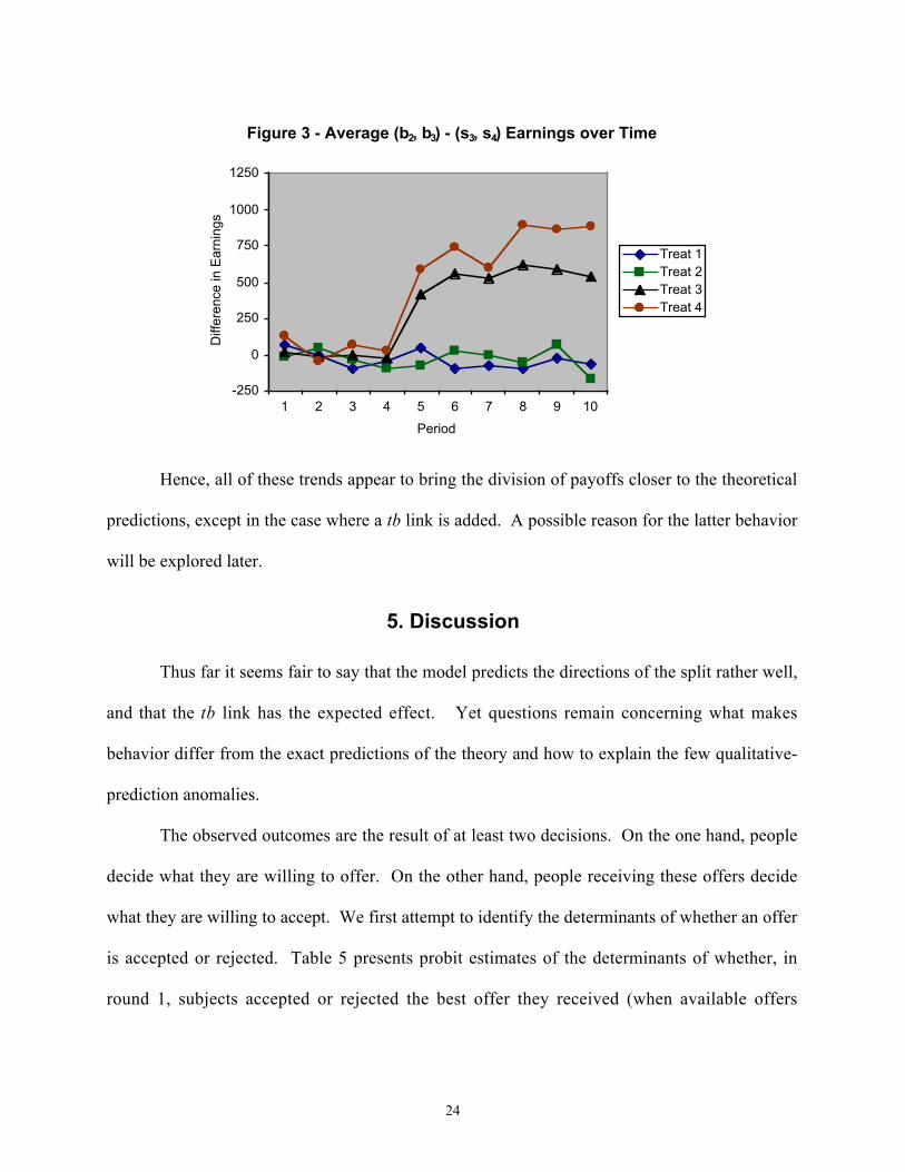
Figure 3 looks at the difference between the average payoffs for the top and the bottom

of the 4-person network. In the first 4 periods, there is very little difference between the average

payoffs for b2 and b3 and the average payoffs for s3 and s4. However, behavior after the new link

is added is very sensitive to whether the link connects b1 and s3 or b2 and s2. In the first case

there is no change, but in the second case b2 and b3 payoffs increase dramatically.

24

Figure 3 - Average (b2, b3) - (s3, s4) Earnings over Time

-250

0

250

500

750

1000

1250

1 2 3 4 5 6 7 8 9 10

Period

Diff

eren

ce in

Ear

ning

s

Treat 1Treat 2Treat 3Treat 4

Hence, all of these trends appear to bring the division of payoffs closer to the theoretical

predictions, except in the case where a tb link is added. A possible reason for the latter behavior

will be explored later.

5. Discussion

Thus far it seems fair to say that the model predicts the directions of the split rather well,

and that the tb link has the expected effect. Yet questions remain concerning what makes

behavior differ from the exact predictions of the theory and how to explain the few qualitative-

prediction anomalies.

The observed outcomes are the result of at least two decisions. On the one hand, people

decide what they are willing to offer. On the other hand, people receiving these offers decide

what they are willing to accept. We first attempt to identify the determinants of whether an offer

is accepted or rejected. Table 5 presents probit estimates of the determinants of whether, in

round 1, subjects accepted or rejected the best offer they received (when available offers

25

differed, the lower one(s) were never chosen).31 Two separate probit regressions are estimated

for the voters, one for type b1 and one for pooled types b2 and b3.32

Table 5 - Determinants for Accepting an Offer

Type b1 Types b2 and b3

(pooled)Share offered (all link types forb1 and no tb link for b2 and b3)

12.95***(3.95)

11.79***(2.40)

Share offered with tb link(for b2 and b3)

-- 8.92***(2.04)

Average share the positionreceived in the past

-13.27***(4.10)

-2.10***(0.77)

2-link -- 0.54**(0.30)

3-link 0.05(0.62)

1.00**(0.46)

Constant 0.97(1.39)

-2.76**(1.21)

Number of Observations 132 264

Log likelihood -37.93 -107.67

Period one omitted *,**,*** indicates statistical significance at p = 0.10, 0.05, 0.01.2-link is a dummy that has a value of 1 if the offerer is linked to 2 people, and is 0 otherwise.3-link is a dummy that has a value of 1 if the offerer is linked to 3 people, and is 0 otherwise.

As expected, the share offered is a significant factor with regard to acceptance or

rejection – higher proposed shares are more likely to be accepted. However, note that b2 and b3

are generally willing to accept less money when there is a tb link. This is a bit surprising, as we

31 In this case, a likelihood ratio test strongly rejects the random-effects specification for b2 and b3 types. Since theresults are not markedly different for b1, we only include the probit in the text and provide the random-effects probitestimates in Appendix E (Table 5b). There were no significant period effects, so these are also omitted in theregression. The results were unaffected.32 Pooling data for positions b2 and b3 may seem incorrect since although they are predicted to be equivalent inequilibrium, they might not be in practice. The extent to which they differ is the number of connections. Thus wecontrol for the number of links even if these are not predicted to have an impact theoretically. Another (separate)issue is that, as shall be seen later, the added link between the two (originally) separate networks, tb and bt, may notbe irrelevant in the laboratory. Hence we have also estimated the probit regressions interacting the share offeredwith a dummy for each type of link. We show that for type b1, none of the three coefficient estimates differstatistically; for types b2 and b3, the cases with no link and with a bt link do not differ statistically, but the coefficientfor the tb link differs from both of the others. This both confirms the theory and validates the specification choicefor the probit regressions.

26

have seen (Tables 2 and 3) that b2 and b3 receive a greater amount with a tb link. It would

appear that this effect must be driven by higher tb-link offers being made. In fact, (s3,s4) round 1

offers average 1366 with a tb link, compared to 1180 with a bt link. A Wilcoxon-Mann-Whitney

test finds that these offers are significantly different, at p = 0.000. Since b2 can reach an

agreement with s2 with a tb link, both s3 and s4 should be concerned with being left unmatched in

this case, and so must compete.

Perhaps more interesting is the fact that the shares allocated in the past affect what one is

willing to accept. Thus, people appear to be learning the social norm for the group.33 Preference

theory presumes that people’s tastes are fixed; however, people may be in unfamiliar situations

(either in the laboratory or in the field), and may be uncertain about appropriate behavior. It is

natural to consider that individuals update their beliefs about social norms on the basis of other

observed outcomes. Yet, to our knowledge, none of the models of learning or social preferences

take this factor into account. Here we see that the higher the average share previously received

by a position, the less likely it is that a person in that position will accept any given offer.

We find that both b1 and (b2,b3) decisions on whether to accept offers are sensitive to

whether the subject is connected to only one person. This is orthogonal to whether or not a tb

link is present, and is not predicted by the theory. However, this factor seems quite plausible

psychologically; perhaps people get more nervous when they only have one connection, and are

correspondingly less aggressive. Also notice that the coefficient for a 3-link is nearly identical

33 Note that this is not the usual form of learning, where agents learn from the agents to whom they are connected.Instead, since agents change positions, they see what other people do in the same position. We find that theirbehavior is influenced by what they observe.

27

to that of the 2-link (it is not statistically different) for b2 and b3, and the coefficient for a 3-link

is effectively zero for b1 decisions.34

The coefficient on average share received is noticeably higher for b1 than is the

coefficient for b2 and b3. However, these are non-linear, so it may be useful for comparison

purposes to compute the marginal effects,35 as shown in Table 6:

Table 6 - Marginal Effects on Determinants for Accepting an Offer

Type b1 Types b2 and b3

(pooled)Share offered (all link types for b1

and no tb link for b2 and b3)1.34***(0.46)

2.81***(0.56)

Share offered with tb link(for b2 and b3)

-- 2.13***(0.46)

Average share the positionreceived in the past

-1.38***(0.49)

-0.50***(0.18)

2-link -- 0.15**(0.09)

3-link 0.01(0.06)

0.15***(0.04)

Period one omitted *,**,*** indicates statistical significance at p = 0.10, 0.05, 0.01.2-link is a dummy that has a value of 1 if the offerer is linked to 2 people, and is 0 otherwise.3-link is a dummy that has a value of 1 if the offerer is linked to 3 people, and is 0 otherwise.

As can be seen, the effect of the past share allocated to a given position is less important

for positions b2 and b3 than for position b1. One potential explanation for this difference is that

the social norm is more salient when there is only one focal point: Player b1 can easily isolate

past b1 outcomes, whereas player b2 or player b3 must divide his or her attention between past b2

and b3 outcomes. In any event, the effect of the past share is strongly statistically significant in

both cases. The effect of having more than one link is substantial. For example, its effect on the

34 Note that b1 is always connected to at least 2 people in the first round of bargaining, which is all we consider inour analysis.35 These were taken at the mean of the regressors except for discrete regressors.

28

probability of acceptance is 0.15, comparable to an increase of 5-7 percentage points from the

mean in the share offered

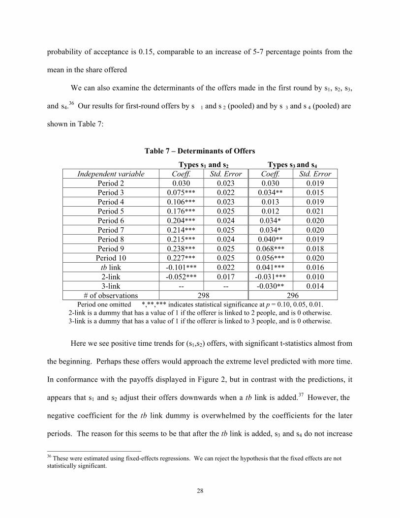
We can also examine the determinants of the offers made in the first round by s1, s2, s3,

and s4.36 Our results for first-round offers by s 1 and s 2 (pooled) and by s 3 and s 4 (pooled) are

shown in Table 7:

Table 7 – Determinants of Offers

Types s1 and s2 Types s3 and s4

Independent variable Coeff. Std. Error Coeff. Std. ErrorPeriod 2 0.030 0.023 0.030 0.019Period 3 0.075*** 0.022 0.034** 0.015Period 4 0.106*** 0.023 0.013 0.019Period 5 0.176*** 0.025 0.012 0.021Period 6 0.204*** 0.024 0.034* 0.020Period 7 0.214*** 0.025 0.034* 0.020Period 8 0.215*** 0.024 0.040** 0.019Period 9 0.238*** 0.025 0.068*** 0.018Period 10 0.227*** 0.025 0.056*** 0.020

tb link -0.101*** 0.022 0.041*** 0.0162-link -0.052*** 0.017 -0.031*** 0.0103-link -- -- -0.030** 0.014

# of observations 298 296Period one omitted *,**,*** indicates statistical significance at p = 0.10, 0.05, 0.01.

2-link is a dummy that has a value of 1 if the offerer is linked to 2 people, and is 0 otherwise.3-link is a dummy that has a value of 1 if the offerer is linked to 3 people, and is 0 otherwise.

Here we see positive time trends for (s1,s2) offers, with significant t-statistics almost from

the beginning. Perhaps these offers would approach the extreme level predicted with more time.

In conformance with the payoffs displayed in Figure 2, but in contrast with the predictions, it

appears that s1 and s2 adjust their offers downwards when a tb link is added.37 However, the

negative coefficient for the tb link dummy is overwhelmed by the coefficients for the later

periods. The reason for this seems to be that after the tb link is added, s3 and s4 do not increase

36 These were estimated using fixed-effects regressions. We can reject the hypothesis that the fixed effects are notstatistically significant.

29

their offers as much as is predicted by theory. This allows s2 to undercut s3 and also allows s1 to

decrease his offers. Note that this also explains the anomalous jump in Figure 2 for Treatments

3 and 4.38 We should also expect s 3 and s4 to adjust their offers, and this is exactly what we see:

A fixed-effect regression (shown in Table 7b, Appendix E) on only the data from treatments

with tb links confirms that s3 and s4 make higher offers after a tb link is added. Every coefficient

is increasing after period 4, and all but the dummy for period 5 are statistically different from the

base period. It seems that s3 and s4 realize that their power has been eroded by the link, but that

it takes some time for the effect to develop.

As with b1 and (b2,b3) offer-acceptance decisions, we find that both (s1,s2) and (s3,s4)

offers are sensitive to whether the subject is connected to only one person.39 This may explain

the surprising result (Table 3) that s3 and s4’s payoffs are not equal. To see this, we will show

that results for networks 2 and 4 (where s3 and b3 have more connections than s2 and b2) drive

the payoff inequality. Also notice that for s3 and s4, the coefficient for a 3-link is nearly identical

to that of the 2-link (it is not statistically different). Table 8 presents some sign test results:

Table 8 – Sign Tests on (s3,s4) and (b2,b3) Payoffs

Link category, Network typenone, N tb, N bt, N none, |X| tb, |X| bt, |X|

s3 vs. s4 r nr r nr nr nrb2 vs. b3 r* nr r nr nr nr

r (nr) means we can (cannot) reject the hypothesis that the payoffs are equal.r* means significant at p = 0.10, but not 0.05.

Our theory predicts that s3 and s4 payoffs should be the same, and b2 and b3 payoffs

should be the same. While s3 and s4 payoffs are not different for the |X| network, they are

37 A sign test indicates that s1 and s2 payoffs are significantly lower before a tb link than after one is made.38 This is also consistent with the observation that b1’s payoffs are higher in treatments 1 and 2 than in treatment 3and 4 (significant at the 1% significance level using a Mann-Whitney test).

30

significantly different in most conditions for the N network.40 As the only real difference

between these networks is the number of connections for s4, it appears that having only a single

connection inspires perceived bargaining weakness. There is a weaker effect for b2 and b3,

perhaps because they are responding to concrete offers rather than proposing offers from a

continuum. Note that none of the six comparisons in the |X| networks show even a marginally

significant difference.

Some modeling and design issues

We have modeled bargaining as an alternating-offer process, with multi-lateral

simultaneous bargaining. We provide full information about the network structure, offers, and

acceptances to every experimental participant. These characteristics are not completely general

to bargaining environments, so we must consider whether our results are artifacts of a

specialized conceptual view.

One concern is that a more unstructured bargaining protocol might lead to different

outcomes, as alternating-offers models may make idiosyncratic predictions about the effects of

outside options in bilateral bargaining and this could carry over to the network structure in the

design.41 While this is a reasonable concern, there is some evidence that the observed results are

somewhat robust to the bargaining protocol. Alsina, Fuertes, Moret & Planell (2000) replicate

our network and payoff structures, but use a double-auction design instead of alternating offers.

All subjects could submit bids in each round. To maintain anonymity, bids were written down

39 Note that for s1 and s2, this simply identifies the different impacts of the link on types.40 Indeed, the only D vs. E comparison that is not significantly different in N networks occurs with a tb link. This isconsistent with our explanation, as here D is being directly undercut by B, and so needs to adjust more (in animmediate sense) than does E.41 We thank Vince Crawford for this observation.

31

on pieces of paper and an experimenter would copy them on the blackboard. Their results were

very close to ours, both with respect to payoffs, treatment effects, and efficiency.

Another issue is that it may be unrealistic to expect bargainers to have the full

information that we provide, limiting the applicability of our results. In principle, each of the

players would seem to need to know the structure of the whole network, as we see that ‘distant’

changes in the trading channels can have major implications for local bargaining outcomes.

However, an agent actually only need know information about the particular subgraph to which

she belongs by the graph decomposition.42 This may not be a burdensome requirement; in fact,

in the small markets/networks mentioned earlier (airplanes, arms, etc.), the limited number of

participants may well know the full information that we provide. The Lovaglia et al. (1995) test

of the effect of restricting this information showed no discernible difference in (late-session)

outcomes, although it took substantially longer to arrive at these outcomes. On an empirical

level, perhaps one only needs to know minimal information about local connections, agreements,

and payoffs.

In line with the Lovaglia et al. (1995) results, we conjecture that the public display of all

information helped to accelerate the learning process, and perhaps served to minimize

disagreements. This additional information may facilitate a common perception of the pertinent

social norm. Blume, DeJong, Kim, and Sprinkle (1998) find that providing a population history

leads to an increase in the proportion of separating outcomes achieved in a sender-receiver

game, and Duffy and Feltovich (1999) find that observation of other players' actions and payoffs

appears to affect the evolution of play. Cooper and Stockman (2001) and Cabrales and Charness

42 Further, giving information on the full network may actually confuse people, and so may not be an unmixedblessing.

32

(1999) present evidence that suggests people learn social norms of punishment in 3-person

games.43

6. Conclusion

We conduct an experiment to study the effect of network structure on bargaining

outcomes in a bipartite market of buyers and sellers of a homogenous and indivisible good. In

many markets, a buyer is connected to only a small subset of all sellers, and vice versa. Such an

interaction can be modeled as a network, which describes the feasible links (trading possibilities)

between agents.

We observe a high degree of bargaining efficiency, in that the total payoffs received are

96% of the maximum possible.44 The public display of all bids and acceptances may accelerate

learning with respect to both bargaining power and group norms about appropriate division.45

While there are only 10 separate bargaining interactions for each individual in an experimental

session, there is strong evidence of substantial changes in bargaining behavior even over this

limited period of time.

In the laboratory, the payoffs do not go the extremes predicted in some cases, as might be

expected given the extensive research on ultimatum and dictator games. Nevertheless, payoffs

are typically asymmetric where predicted so, and in the expected direction. We find that the

manner in which a new link between two groups is made does lead to sharply different behavior,

43 However, Sell and Wilson (1991) and Croson (1997) find that providing information about individualcontributions (VCM) did not lead to either a higher contribution level or a reduction of the group variance.44 It is true that the high degree of efficiency may be partially an artifact of the modest decline in payoffs withsuccessive bargaining rounds. Nevertheless, efficiency would still be quite high (92%) with the same bargainingbehavior and a (for example) 20% discount from round to round, since 75% of the possible agreements are reachedin the first round, and 17% in the 2nd round. A steeper discount rate could also induce more rapid agreement,partially compensating for the higher efficiency loss from round to round.45 Chatterjee and Dutta (1998) find that public offers in thin markets lead to a unique subgame-perfect equilibrium inpure strategies, whereas private offers do not permit any efficient equilibria in pure strategies.

33

even for bargainers not directly involved with the new link. It is perhaps surprising that we find

these effects in such a short time in such a complex environment.

We do find some unexpected regularities in our data, such as the difference between s3

and s4 payoffs (and b2 and b3 payoffs) in N networks, and an anomalous jump in s1 and s2

earnings after a tb link is added. We see some explanations outside of the bargaining model,

such as a significant decrease in earnings when an agent is connected to only one other agent,

even where an extra connection (in the N network) should not make any difference. This

indicates that what makes the results from the |X| network look so similar to what has been

observed before in multilateral bargaining game is not simply the fact that there is the same

numbers of buyers and sellers connected together, but also that they all have the same number of

connections.

We find strong evidence of a form of social learning: The shares allocated in the past to

one’s neighbors affect what one is willing to accept. Individuals learn from the actions of others,

and groups seem to develop social norms for bargaining choices. This phenomenon could be the

result of subjects updating their beliefs about the success of different strategies as in belief-based

learning models (Fudenberg and Levine 1999); it could also be a more general form of social

learning, where subjects are trying to learn the acceptable norm by observing the behavior of

others (see Ellison 2002, for example). In any case, this behavior has important implications for

models of social preferences and learning.

We cannot readily disentangle whether the effects are induced by strategic considerations

(maximizing one’s expected monetary payoff) or fairness constraints on lopsided divisions.

Since we do observe substantial deviations from the theoretical point predictions for extreme

allocations, the fairness explanation immediately comes to mind. However, note that b1 earnings

34

seem to be approaching the 2300 predicted in the last periods of Treatments 1 and 2. Perhaps

the deviation is a transient phenomenon, and the social norm is a moving target. It seems likely

that both profit-maximization and equity considerations are factors at play.

There are many potential applications for network analysis and our results have

implications for network formation and design. We feel that the network framework is a useful

metaphor for many market environments. Natural extensions of our work include changing

bargaining timing and protocols, as well as considering endogenous link-formation with bipartite

markets. For example, if we consider that it may be possible to add or subtract links in markets,

we can predict the effect of such changes in the trading regime.46 It is plausible that the lower

payoffs experienced by people with few links could lead to over-connectedness, from a social

standpoint. As network theory is still evolving and general solutions are often unobtainable,

experimental study seems a very natural complement in this emerging area.

46 For example, suppose there is a tb link in existence and s2 can sever it. b2 and b3 would pay s2 to do so, but wouldbe bidding against s3 and s4.

35

References

Alsina, A., R. Fuertes, E. Moret & M. Planell (2000) “Doble Subhasta amb Xarxes (Double Auctionwith Networks),” mimeo, Universitat Pompeu Fabra.

Bala, V. and S. Goyal (2000), “A Non-Cooperative Theory of Network Formation,” Econometrica,68, 1181-1229.

Bala, V. and S. Goyal (1998), “Learning from Neighbours,” Review of Economic Studies, 65,595-621.

Berninghaus, S., K. Ehrhart & C. Keser (1998), “Coordination and Local Interaction: ExperimentalEvidence, Economics Letters, 58, 269-75.

Blume, A., D. DeJong, Y. Kim & G. Sprinkle (1998), “Experimental Evidence on the Evolutionof Meaning of Messages in Sender-Receiver Games,” American Economic Review, 88,1323-1340.

Bolton, G., K. Chatterjee & K. Valley (2001), “How Communication Links Influence CoalitionBargaining - A Laboratory Investigation.” mimeo.

Boorman, S. (1975), “A Combinatorial Optimization Model for Transmission of Job Informationthrough Contact Networks,” Bell Journal of Economics, 6, 216-249.

Burt, R. (2000), “The Network Structure of Social Capital,” forthcoming in Research inOrganizational Behavior, R. Sutton and B. Staw, eds.

Cabrales, A. and G. Charness (1999), “Optimal Contracts, Adverse Selection, and Social Preferences:An Experiment,” mimeo.

Calvó-Armengol, A. (2001a), “Bargaining Power in Communication Networks,” MathematicalSocial Sciences, 41, 69-87.

Calvó-Armengol, A. (2001b), “Job Contact Networks,” mimeo.Camerer, C. and R. Weber (2001), “Cultural Conflict and Merger Failure: An Experimental

Approach,” mimeo.Cassar, A. (2002), “Coordination and Cooperation in Local, Random, and Small World Networks:

Experimental Evidence,” in Proceedings of the 2002 North American Summer Meetings of theEconometric Society: Game Theory, D. Levine, W. Zame, L. Ausubel, P._A. Chiappori,B. Ellickson, . Rubinstein, and L. Samuelson, eds.

Charness, G. (2000), “Bargaining Efficiency and Screening: An Experimental Investigation,”Journal of Economic Behavior and Organization, 42, 285-304.

Chatterjee, K. and B. Dutta (1998), “Rubinstein Auctions: On Competition for Bargaining Partners,”Games and Economic Behavior, 23, 119-145.

Chwe, M. (2000), “Communication and Coordination in Social Networks,” Review of EconomicStudies, 67, 1-16.

Cochran, W. (1977), Sampling Techniques, 3rd ed., New York: John Wiley & Sons.Cook, K. and R. Emerson (1978), “Power, Equity, and Commitment in Exchange Networks,”

American Sociological Review, 43, 721-39.Cooper, D. and C. Stockman (2001), “Learning to Punish: Experimental Evidence from a

Sequential Step-Level Public Goods Game,” mimeo.Corbae, D. and J. Duffy (2001), “Experiments with Network Economies,” mimeo.Corominas-Bosch, M. (1999), “On Two-sided Network Markets,” Ph.D. Thesis, Universitat Pompeu

Fabra.Corominas-Bosch, M. (forthcoming), “Bargaining in a Network of Buyers and Sellers,” Journal of

Economic Theory.Crawford, V. and S. Rochford (1986), “Bargaining and Competition in Matching Markets,”

International Economic Review 27, 329-48.Croson, R. (1997), “Feedback in Voluntary Contribution Mechanisms: An Experiment in Team

Production,” forthcoming in Research in Experimental Economics.

36

Deck, C. and C. Johnson (2002), “Link Bidding in a Laboratory Experiment,” mimeo.Duffy, J. and N. Feltovich (1999), “Does Observation of Others Affect Learning in Strategic

Environments? An Experimental Study,” International Journal of Game Theory, 28,131-152.

Edmonds, J. (1965), “Paths, Trees and Flowers,” Canadian Journal of Mathematics, 17, 449-467.Ellison, G. (2002), “Evolving Standards for Academic Publishing: A q-r Theory,” Journal of Political

Economy, 110, 994-1034.Ellison, G. and D. Fudenberg (1993), “Rules of Thumb for Social Learning,” Journal of Political

Economy, 101, 612-43.Ellison, G. and D. Fudenberg (1995), “Word-of-Mouth Communication and Social Learning,”

Quarterly Journal of Economics, 110, 93-125.Falk, A. and M. Kosfeld (2003), “It’s All about Connections: Evidence on Network Formation,” mimeo.Fudenberg D. and D. Levine (1999), Learning and Evolution in Games, The MIT Press: Cambridge,

Massachusetts.Gale, D. (1987), “Limit Theorems for Markets with Sequential Bargaining,” Journal of Economic

Theory, 43, 20-54.Gale, D. and L. Shapley (1962), “College Admissions and the Stability of Marriage,” American

Mathematical Monthly, 69, 9-15.Gallai, T (1963), “Kritische Graphen II,” Magyar Tud. Akad. Mat. Kutató Int. Közl, 8, 373-395

(in Hungarian).Gallai, T. (1964), “Maximale Systeme unabhängiger Kanten,” Magyar Tud. Akad. Mat. Kutató

Int. Közl , 9, 401-413 (in Hungarian).Glaeser, E., B. Sacerdote & J. Sheinkman (1996), “Crime and Social Interactions,” Quarterly Journal

of Economics, 111, 507-48.Gould, R. (1988), Graph Theory, Menlo Park, CA: The Benjamin/Cummings Publishing Co., Inc.Guseva, A. and A. Rona-Tas (2001), “Uncertainty, Risk, and Trust: Russian and American Credit

Card Markets Compared,” American Sociological Review, 66, 623-646.Hall, P. (1935), “On Representatives of Subsets” Journal of London Mathematical Society, 10,

26-30.Hendricks, K., M. Piccione & G. Tan (1995), “The Economics of Hubs: The Case of Monopoly,”

Review of Economic Studies, 62, 83-100.Jackson, M. and A. Watts (1998), “The Evolution of Social and Economic Networks,” mimeo.Jackson, M. and A. Wolinsky (1996), “A Strategic Model of Social and Economic Networks,”

Journal of Economic Theory, 71, 44-74.Jackson, M. and E. Kalai (1997), “Social Learning in Recurring Games,” Games and Economic

Behavior, 21, 102-34.Jackson, M. and E. Kalai (1999), “Reputation vs. Social Learning,” Journal of Economic Theory, 85,

40-59.Katz, M. and C. Shapiro (1994), Systems Competition and Network Effects,” Journal of Economic

Perspectives, 8, 93-115.Kelso, A. and V. Crawford (1982), “Job Matching, Coalition Formation, and Gross Substitutes,”

Econometrica, 25, 1483-1504.Kirchkamp, O. and R. Nagel (forthcoming), “Repeated Game Strategies in Local and Group

Prisoner’s Dilemmas Experiments: First Results,” Homo Oeconomicus.Kosfeld, M. (2003), “Network Experiments,” mimeo.Kranton, R. and D. Minehart (2001), “A Theory of Buyer-Seller Networks,” American Economic

Review, 91, 485-508.Lamoureaux, N. (1986), “Banks, Kinship, and Economic Development: The New England Case,”

Journal of Economic History, 46, 647-667.Lovaglia, M., J. Skvoretz, D. Willer, and B. Markovsky (1995), “Negotiated Exchanges in Social

Networks,” Social Forces, 74, 123-55.

37

Lovasz, L. and M. Plummer (1986), Matching Theory, New York: North-Holland.Markovsky, B., D. Willer, and T. Patton (1988), “Power Relations in Exchange Networks,”

American Sociological Review, 53, 220-36.Montgomery, J. (1991), “Social Networks and Labor Market Outcomes: Toward an Economic

Analysis,” American Economic Review, 81, 1408-1418.Morris, S. (2000), “Contagion,” Review of Economic Studies, 67, 67-78.Palomino, F. and F. Vega-Redondo (1999), “Convergence of Aspirations and (Partial) Cooperation

in the Prisoner’s Dilemma,” International Journal of Game Theory, 28, 465-488.Riedl, A. and A. Ule (2002), “Exclusion and Cooperation in Social Network Experiments,” mimeo.Roth, A. (1984), “Stability and Polarization of Interests in Job Matching,” Econometrica, 52, 47-57.Roth A. (1995), “Bargaining Experiments”, in Handbook of Experimental Economics, J. Kagel and

A. Roth (editors), Princeton University Press, Princeton, 253-348.Roth, A., V. Prasnikar, M. Okuno-Fujiwara & S. Zamir (1991), “Bargaining and Market Behavior in

Jerusalem, Ljubljana, Pittsburgh, and Tokyo: An Experimental Study, American EconomicReview, 81, 1068-95.

Roth, A. and M. Sotomayor (1989), “Two-sided Matching,” Econometric Society Monographs 18,Cambridge: Cambridge University Press.

Rubinstein, A. (1982), “Perfect Equilibrium in a Bargaining Model,” Econometrica, 50, 97-110.Sell, J. and R. Wilson (1991), “Levels of Information and Contributions to Public Goods,” Social

Forces, 70, 107-24.Shapley. L. and M. Shubik (1972), "The Assignment Game I: The Core,” International Journal of

Game Theory 1, 111-30.Skvoretz, J. and D. Willer (1991), “Power in Exchange Networks: Setting and Structure Variations,”

Social Psychology Quarterly, 54, 224-38.Stolte, J. and R. Emerson (1977), “Structural Inequality: Position and Power in Exchange Structures,”

in Behavioral Theory in Sociology, R. Hamblin & J. Kunkel, eds., New Brunswick, NJ:Transaction Books, 117-38.

Topa, G. (1999), “Social Interactions, Local Spillovers, and Unemployment,” mimeo.Valley, K., and T. Thompson (1998), “Sticky Ties and Bad Attitudes: Relational and Individual Bases

of Resistance to Changes in Organizational Structure,” in Power, Politics and Influence, R.Kramer and M. Neale, eds., Thousand Oaks, Calif.: Sage.

Willer, D., M. Lovaglia, and B. Markovsky (1997), “Power and Influence: A Theoretical Bridge,”Social Forces, 76, 571-604.

Willer, D. (1999), Network Exchange Theory, New York: Praeger.Wolter, K. (1985), Introduction to Variance Estimation, New York: Springer-Varlag.

38

Appendix A – Graph Theory Notation and Results

We now start introducing basic concepts in graph theory. All concepts are standard (excepting the definition of GS,GB, and GE) and can be found in any graph theory textbook, e.g., Gould (1988).

A non-directed bipartite graph G=<S»B,L> consists of a set of nodes, formed by n sellers S={s1,..., sn } and mbuyers B={ b1,..., bm}, and a set of links L, each link joining a seller with a buyer. An element of L, say a link fromsi to bj will be denoted as si : bj.

A subgraph G0=<S0»B0,L0> of G=<S»B,L> is a graph such that S0ÕS, B0ÕB, L0ÕL, and such that each link in L0

connects a seller of S0 with a buyer in B0. When we speak of the subgraph G0 induced by the set of nodes S0»B0 inG we mean the subgraph formed by the nodes S0»B0 and all the links that connect a seller in S0 and a buyer in B0 inG.

A matching in a bipartite graph G=<S»B,L> is a collection of pairs of linked members of B and S such that eachagent in S»B belongs to at most one pair. We say that a subset of agents can be matched if there exists a matchinginvolving these agents.

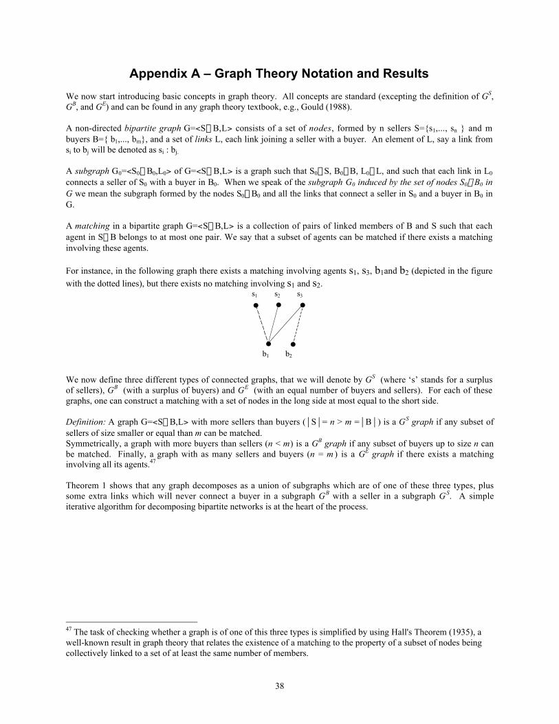
For instance, in the following graph there exists a matching involving agents s1, s3, b1and b2 (depicted in the figure

with the dotted lines), but there exists no matching involving s1 and s2.s1 s2 s3

b1 b2

We now define three different types of connected graphs, that we will denote by GS (where ‘s’ stands for a surplusof sellers), GB (with a surplus of buyers) and GE (with an equal number of buyers and sellers). For each of thesegraphs, one can construct a matching with a set of nodes in the long side at most equal to the short side.

Definition: A graph G=<S»B,L> with more sellers than buyers (S= n > m =B) is a GS graph if any subset ofsellers of size smaller or equal than m can be matched.Symmetrically, a graph with more buyers than sellers (n < m) is a GB graph if any subset of buyers up to size n canbe matched. Finally, a graph with as many sellers and buyers (n = m ) is a GE graph if there exists a matchinginvolving all its agents.47

Theorem 1 shows that any graph decomposes as a union of subgraphs which are of one of these three types, plussome extra links which will never connect a buyer in a subgraph GB with a seller in a subgraph GS. A simpleiterative algorithm for decomposing bipartite networks is at the heart of the process.

47 The task of checking whether a graph is of one of this three types is simplified by using Hall's Theorem (1935), awell-known result in graph theory that relates the existence of a matching to the property of a subset of nodes beingcollectively linked to a set of at least the same number of members.

39

Theorem 1

1) Every graph G can be decomposed into a number of subgraphs GS1 ,...,G

SnS (of the GS type), GB

1 ,...,GB

nB (ofthe GB type), GE

1 ,...,GEnE (of the GS type), such that each node of G belongs to one and only one of the

subgraphs and any seller (buyer) in a GSi (G

Bi ) is only linked to buyers (sellers) in a GS

j (GB

j ).2) Moreover, a given node always belongs to the same type of subgraph for any such decomposition.We will write G= GS

1 » ... » GSnS » GB

1 » ... » GBnB » GE

1 » ... » GEnE, with the union being disjoint.

Proof: See Corominas-Bosch (forthcoming)

We can adapt the theory to the particular networks used in our design: applying Theorem 1 to the networks used inthe experiment, we get the following decompositions:

(1) (2) (3)

GSGE GE

(4) (5)

GSGE GS

GE

(6) (7)

GS GS

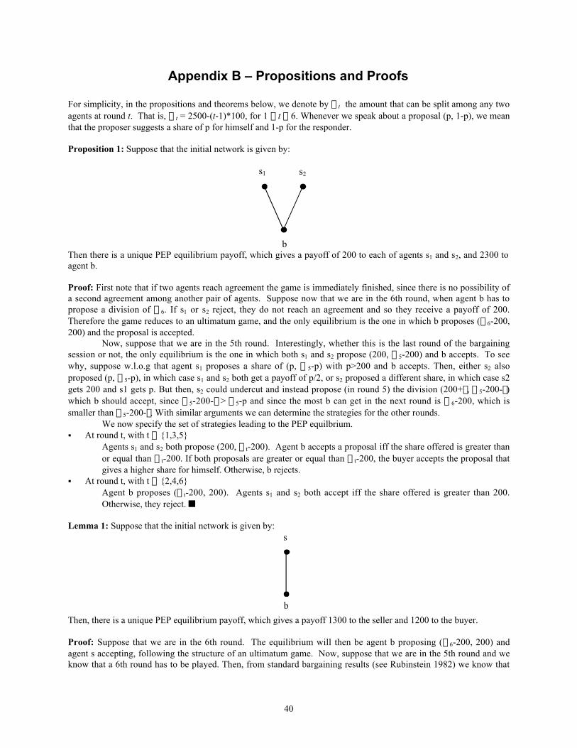
40

Appendix B – Propositions and Proofs

For simplicity, in the propositions and theorems below, we denote by Pt the amount that can be split among any twoagents at round t. That is, Pt = 2500-(t-1)*100, for 1 £ t £ 6. Whenever we speak about a proposal (p, 1-p), we meanthat the proposer suggests a share of p for himself and 1-p for the responder.

Proposition 1: Suppose that the initial network is given by:

s1

b

s2

Then there is a unique PEP equilibrium payoff, which gives a payoff of 200 to each of agents s1 and s2, and 2300 toagent b.

Proof: First note that if two agents reach agreement the game is immediately finished, since there is no possibility ofa second agreement among another pair of agents. Suppose now that we are in the 6th round, when agent b has topropose a division of P6. If s1 or s2 reject, they do not reach an agreement and so they receive a payoff of 200.Therefore the game reduces to an ultimatum game, and the only equilibrium is the one in which b proposes (P6-200,200) and the proposal is accepted.

Now, suppose that we are in the 5th round. Interestingly, whether this is the last round of the bargainingsession or not, the only equilibrium is the one in which both s1 and s2 propose (200, P5-200) and b accepts. To seewhy, suppose w.l.o.g that agent s1 proposes a share of (p, P5-p) with p>200 and b accepts. Then, either s2 alsoproposed (p, P5-p), in which case s1 and s2 both get a payoff of p/2, or s2 proposed a different share, in which case s2gets 200 and s1 gets p. But then, s2 could undercut and instead propose (in round 5) the division (200+e, P5-200-e)which b should accept, since P5-200-e > P5-p and since the most b can get in the next round is P6-200, which issmaller than P5-200-e. With similar arguments we can determine the strategies for the other rounds.

We now specify the set of strategies leading to the PEP equilbrium.ß At round t, with t Œ {1,3,5}

Agents s1 and s2 both propose (200, Pt-200). Agent b accepts a proposal iff the share offered is greater thanor equal than Pt-200. If both proposals are greater or equal than Pt-200, the buyer accepts the proposal thatgives a higher share for himself. Otherwise, b rejects.

ß At round t, with t Œ {2,4,6}Agent b proposes (Pt-200, 200). Agents s1 and s2 both accept iff the share offered is greater than 200.Otherwise, they reject. n

Lemma 1: Suppose that the initial network is given by: s

b

Then, there is a unique PEP equilibrium payoff, which gives a payoff 1300 to the seller and 1200 to the buyer.

Proof: Suppose that we are in the 6th round. The equilibrium will then be agent b proposing (P6-200, 200) andagent s accepting, following the structure of an ultimatum game. Now, suppose that we are in the 5th round and weknow that a 6th round has to be played. Then, from standard bargaining results (see Rubinstein 1982) we know that

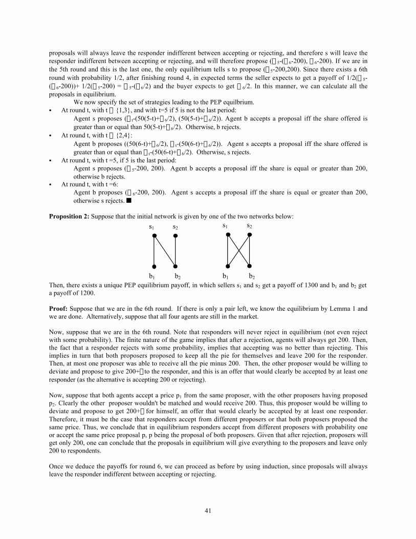
41

proposals will always leave the responder indifferent between accepting or rejecting, and therefore s will leave theresponder indifferent between accepting or rejecting, and will therefore propose (P5-(P6-200), P6-200). If we are inthe 5th round and this is the last one, the only equilibrium tells s to propose (P5-200,200). Since there exists a 6thround with probability 1/2, after finishing round 4, in expected terms the seller expects to get a payoff of 1/2(P5-(P6-200))+ 1/2(P5-200) = P5-(P6/2) and the buyer expects to get P6/2. In this manner, we can calculate all theproposals in equilibrium.

We now specify the set of strategies leading to the PEP equilbrium.ß At round t, with t Œ {1,3}, and with t=5 if 5 is not the last period:

Agent s proposes (Pt-(50(5-t)+P6/2), (50(5-t)+P6/2)). Agent b accepts a proposal iff the share offered isgreater than or equal than 50(5-t)+P6/2). Otherwise, b rejects.

ß At round t, with t Œ {2,4}:Agent b proposes ((50(6-t)+P6/2), Pt-(50(6-t)+P6/2)). Agent s accepts a proposal iff the share offered isgreater than or equal than Pt-(50(6-t)+P6/2). Otherwise, s rejects.

ß At round t, with t =5, if 5 is the last period:Agent s proposes (P5-200, 200). Agent b accepts a proposal iff the share is equal or greater than 200,otherwise b rejects.

ß At round t, with t =6:Agent b proposes (P6-200, 200). Agent s accepts a proposal iff the share is equal or greater than 200,otherwise s rejects. n

Proposition 2: Suppose that the initial network is given by one of the two networks below:

s1 s2

b1 b2

s1 s2

b1 b2

Then, there exists a unique PEP equilibrium payoff, in which sellers s1 and s2 get a payoff of 1300 and b1 and b2 geta payoff of 1200.

Proof: Suppose that we are in the 6th round. If there is only a pair left, we know the equilibrium by Lemma 1 andwe are done. Alternatively, suppose that all four agents are still in the market.

Now, suppose that we are in the 6th round. Note that responders will never reject in equilibrium (not even rejectwith some probability). The finite nature of the game implies that after a rejection, agents will always get 200. Then,the fact that a responder rejects with some probability, implies that accepting was no better than rejecting. Thisimplies in turn that both proposers proposed to keep all the pie for themselves and leave 200 for the responder.Then, at most one proposer was able to receive all the pie minus 200. Then, the other proposer would be willing todeviate and propose to give 200+e to the responder, and this is an offer that would clearly be accepted by at least oneresponder (as the alternative is accepting 200 or rejecting).

Now, suppose that both agents accept a price p1 from the same proposer, with the other proposers having proposedp2. Clearly the other proposer wouldn't be matched and would receive 200. Thus, this proposer would be willing todeviate and propose to get 200+e for himself, an offer that would clearly be accepted by at least one responder.Therefore, it must be the case that responders accept from different proposers or that both proposers proposed thesame price. Thus, we conclude that in equilibrium responders accept from different proposers with probability oneor accept the same price proposal p, p being the proposal of both proposers. Given that after rejection, proposers willget only 200, one can conclude that the proposals in equilibrium will give everything to the proposers and leave only200 to respondents.

Once we deduce the payoffs for round 6, we can proceed as before by using induction, since proposals will alwaysleave the responder indifferent between accepting or rejecting.

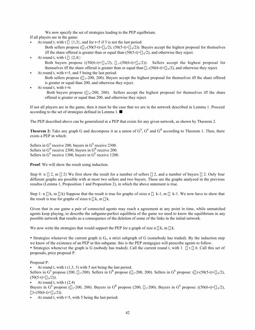
42

We now specify the set of strategies leading to the PEP equilbrium.If all players are in the game:ß At round t, with t Œ {1,3}, and for t=5 if 5 is not the last period:

Both sellers propose (Pt-(50(5-t)+P6/2), (50(5-t)+P6/2)). Buyers accept the highest proposal for themselvesiff the share offered is greater than or equal than (50(5-t)+P6/2), and otherwise they reject.

ß At round t, with t Œ {2,4}:Both buyers propose ((50(6-t)+P6/2), P t-(50(6-t)+P6/2)). Sellers accept the highest proposal forthemselves iff the share offered is greater than or equal than Pt-(50(6-t)+P6/2), and otherwise they reject.

ß At round t, with t=5, and 5 being the last period:Both sellers propose (P5-200, 200). Buyers accept the highest proposal for themselves iff the share offeredis greater or equal than 200, and otherwise they reject.

ß At round t, with t=6:Both buyers propose (P6-200, 200). Sellers accept the highest proposal for themselves iff the share

offered is greater or equal than 200, and otherwise they reject.

If not all players are in the game, then it must be the case that we are in the network described in Lemma 1. Proceedaccording to the set of strategies defined in Lemma 1. n

The PEP described above can be generalized in a PEP that exists for any given network, as shown by Theorem 2.

Theorem 2: Take any graph G and decompose it as a union of GS, GE and GB according to Theorem 1. Then, thereexists a PEP in which:

Sellers in GS receive 200, buyers in GS receive 2300.Sellers in GB receive 2300, buyers in GB receive 200.Sellers in GE receive 1300, buyers in GE receive 1200.

Proof: We will show the result using induction.

Step 0: n £ 2, m £ 2) We first show the result for a number of sellers £ 2, and a number of buyers £ 2. Only fourdifferent graphs are possible with at most two sellers and two buyers. These are the graphs analyzed in the previousresultss (Lemma 1, Proposition 1 and Proposition 2), in which the above statement is true.

Step 1: n £ k, m £ k) Suppose that the result is true for graphs of sizes n £ k-1, m £ k-1. We now have to show thatthe result is true for graphs of sizes n £ k, m £ k.

Given that in our game a pair of connected agents may reach a agreement at any point in time, while unmatchedagents keep playing, to describe the subgame-perfect equilibria of the game we need to know the equilibrium in anypossible network that results as a consequence of the deletion of some of the links in the initial network.

We now write the strategies that would support the PEP for a graph of size n £ k, m £ k.

• Strategies whenever the current graph is Gi, a strict subgraph of G (somebody has traded). By the induction stepwe know of the existence of an PEP in this subgame. this is the PEP stratgegies will prescribe agents to follow.• Strategies whenever the graph is G (nobody has traded). Call the current round t, with 1 £ t £ 6. Call this set ofproposals, price proposal P.

Proposal P:ß At round t, with t (1,3, 5) with 5 not being the last period.Sellers in GS propose (200, Pt-200). Sellers in GB propose (Pt-200, 200). Sellers in GE propose: (Pt-(50(5-t)+P6/2),(50(5-t)+P6/2)).ß At round t, with t (2,4)Buyers in GS propose (Pt-200, 200). Buyers in GB propose (200, Pt-200). Buyers in GE propose: ((50(6-t)+P6/2),Pt-(50(6-t)+P6/2)).ß At round t, with t=5, with 5 being the last period:

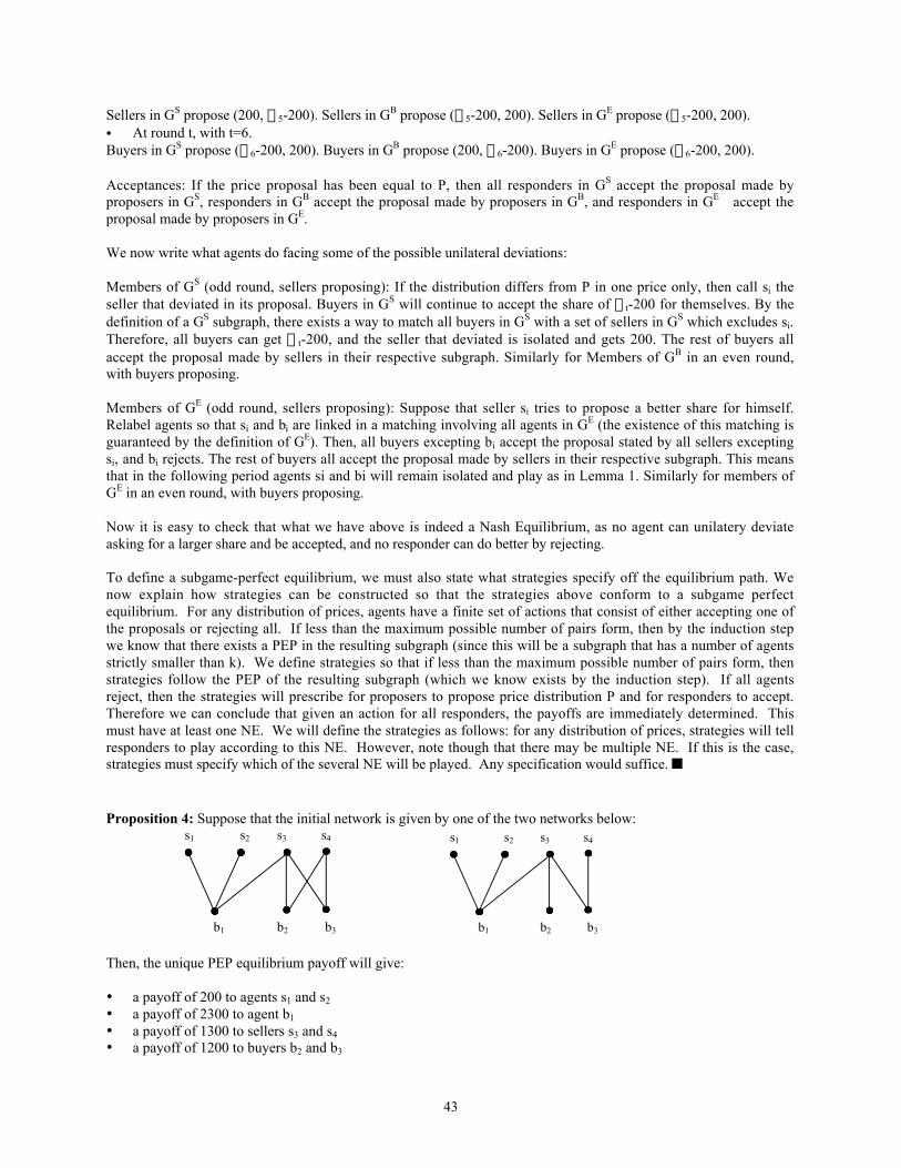
43

Sellers in GS propose (200, P5-200). Sellers in GB propose (P5-200, 200). Sellers in GE propose (P5-200, 200).ß At round t, with t=6.Buyers in GS propose (P6-200, 200). Buyers in GB propose (200, P6-200). Buyers in GE propose (P6-200, 200).

Acceptances: If the price proposal has been equal to P, then all responders in GS accept the proposal made byproposers in GS, responders in GB accept the proposal made by proposers in GB, and responders in GE accept theproposal made by proposers in GE.

We now write what agents do facing some of the possible unilateral deviations:

Members of GS (odd round, sellers proposing): If the distribution differs from P in one price only, then call si theseller that deviated in its proposal. Buyers in GS will continue to accept the share of Pt-200 for themselves. By thedefinition of a GS subgraph, there exists a way to match all buyers in GS with a set of sellers in GS which excludes si.Therefore, all buyers can get Pt-200, and the seller that deviated is isolated and gets 200. The rest of buyers allaccept the proposal made by sellers in their respective subgraph. Similarly for Members of GB in an even round,with buyers proposing.

Members of GE (odd round, sellers proposing): Suppose that seller si tries to propose a better share for himself.Relabel agents so that si and bi are linked in a matching involving all agents in GE (the existence of this matching isguaranteed by the definition of GE). Then, all buyers excepting bi accept the proposal stated by all sellers exceptingsi, and bi rejects. The rest of buyers all accept the proposal made by sellers in their respective subgraph. This meansthat in the following period agents si and bi will remain isolated and play as in Lemma 1. Similarly for members ofGE in an even round, with buyers proposing.

Now it is easy to check that what we have above is indeed a Nash Equilibrium, as no agent can unilatery deviateasking for a larger share and be accepted, and no responder can do better by rejecting.

To define a subgame-perfect equilibrium, we must also state what strategies specify off the equilibrium path. Wenow explain how strategies can be constructed so that the strategies above conform to a subgame perfectequilibrium. For any distribution of prices, agents have a finite set of actions that consist of either accepting one ofthe proposals or rejecting all. If less than the maximum possible number of pairs form, then by the induction stepwe know that there exists a PEP in the resulting subgraph (since this will be a subgraph that has a number of agentsstrictly smaller than k). We define strategies so that if less than the maximum possible number of pairs form, thenstrategies follow the PEP of the resulting subgraph (which we know exists by the induction step). If all agentsreject, then the strategies will prescribe for proposers to propose price distribution P and for responders to accept.Therefore we can conclude that given an action for all responders, the payoffs are immediately determined. Thismust have at least one NE. We will define the strategies as follows: for any distribution of prices, strategies will tellresponders to play according to this NE. However, note though that there may be multiple NE. If this is the case,strategies must specify which of the several NE will be played. Any specification would suffice. n

Proposition 4: Suppose that the initial network is given by one of the two networks below:s1

b1

s2 s3 s4

b2 b3

s1

b1

s2 s3 s4

b2 b3

Then, the unique PEP equilibrium payoff will give:

• a payoff of 200 to agents s1 and s2

• a payoff of 2300 to agent b1

• a payoff of 1300 to sellers s3 and s4

• a payoff of 1200 to buyers b2 and b3

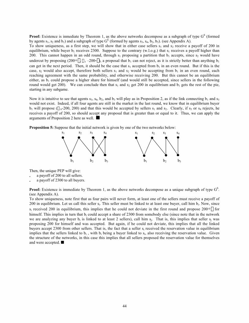
44

Proof: Existence is inmediate by Theorem 1, as the above networks decompose as a subgraph of type GS (formedby agents s1, s2 and b1) and a subgraph of type GE (formed by agents s3, s4, b2, b3). (see Appendix A).To show uniqueness, as a first step, we will show that in either case sellers s1 and s2 receive a payoff of 200 inequilibrium, while buyer b1 receives 2300. Suppose to the contrary (w.l.o.g.) that s1 receives a payoff higher than200. This cannot happen in an odd round, through s1 proposing a partition that b1 accepts, since s2 would haveundercut by proposing (200+e, Pt –200-e), a proposal that b1 can not reject, as it is strictly better than anything b1

can get in the next period. Then, it should be the case that s1 accepted from b1 in an even round. But if this is thecase, s2 would also accept, therefore both sellers s1 and s2 would be accepting from b1 in an even round, eachreaching agreement with the same probability, and otherwise receiving 200. But this cannot be an equilibriumeither, as b1 could propose a higher share for himself (and would still be accepted, since sellers in the followinground would get 200). We can conclude then that s1 and s2 get 200 in equilibrium and b1 gets the rest of the pie,starting in any subgame.

Now it is intuitive to see that agents s3, s4, b2, and b3 will play as in Proposition 2, as if the link connecting b1 and s3

would not exist. Indeed, if all four agents are still in the market in the last round, we know that in equilibrium buyerb1 will propose (P6-200, 200) and that this would be accepted by sellers s1 and s2. Clearly, if s3 or s4 rejects, hereceives a payoff of 200, so should accept any proposal that is greater than or equal to it. Thus, we can apply thearguments of Proposition 2 here as well. n

Proposition 5: Suppose that the initial network is given by one of the two networks below:s1

b1

s2 s3 s4

b2 b3

s1

b1

s2 s3 s4

b2 b3

Then, the unique PEP will give:• a payoff of 200 to all sellers.• a payoff of 2300 to all buyers.

Proof: Existence is immediate by Theorem 1, as the above networks decompose as a unique subgraph of type GS.(see Appendix A).To show uniqueness, note first that as four pairs will never form, at least one of the sellers must receive a payoff of200 in equilibrium. Let us call this seller si. This seller must be linked to at least one buyer, call him bi. Now, sincesi received 200 in equilibrium, this implies that he could not deviate in the first round and propose 200+e forhimself. This implies in turn that bi could accept a share of 2300 from somebody else (since note that in the networkwe are analyzing any buyer bi is linked to at least 2 sellers), call him sj. That is, this implies that seller sj wasproposing 200 for himself and was accepted. But again, if he could not deviate, this implies that all the linkedbuyers accept 2300 from other sellers. That is, the fact that a seller si received the reservation value in equilibriumimplies that the sellers linked to bi , with bi being a buyer linked to si, also receiving the reservation value. Giventhe structure of the networks, in this case this implies that all sellers proposed the reservation value for themselvesand were accepted. n

45

Appendix C - Instructions

Thank you for participating in this experiment. You will receive 500 pesetas for attending the session andappearing on time. In addition, you will make decisions for which you will receive an amount of money;the amount depends on the choices made in the experiment. You will receive a subject number that wewill use to identify you during the experiment. Please hold on to this number, as we will need it in orderto pay you.

In this experiment, you will be in a group of 7 persons who will engage in anonymous bargainingsessions. As explained below, people will make proposals to divide a sum of money between them. Ineach session, every person will be connected to one or more other persons. You can only bargain withthose people with whom you are connected. An individual can only reach an agreement with at most oneother person in a bargaining session.

An example of a diagram of a network (the overall set of possible connections between people) is shownon the board. A network has two sides, a top and a bottom.

Your connection(s) will be constant throughout a bargaining session; however, there will be multiplebargaining sessions and your location on the network may change from one session to the next. Thenetwork itself will remain constant for some number of bargaining sessions, but the network will changeat some point in the experiment. You will be informed when this occurs and a diagram of the newnetwork will be displayed on the board.

Each bargaining session will consist of up to 5 or 6 rounds, each of which consists of two parts. In the 1stpart of the 1st round, each member of the top side of the network will make a proposal for dividing a sumof money with anyone on the bottom side of the network with whom he or she is connected. A proposalis a suggestion of how much money you would receive and how much money a person accepting theproposal would receive. In the 2nd part of the 1st round, individuals on the bottom side of the networkrespond to the proposals made by those individuals with whom they are connected. One may choose toaccept one of these proposals or choose to reject all available proposals. If a proposal is accepted, there isa match and both parties to the match are removed from the network for the remainder of that bargainingsession. If there are no more possible matches that can be made, the bargaining session has beencompleted.

If there are still possible matches, we continue to a 2nd round. In the 1st part of the 2nd round, allpersons on the bottom side of the network who have not become matched will make proposals to divide a(smaller) sum of money with connected persons on the top side of the network. In the 2nd part of the 2ndround, each unmatched individual on the top side of the network will choose either to accept one of theproposals made by people with whom he or she is connected or to reject all available proposals. Matchesare determined and displayed. Once again, if there are no more possible matches to be made, thebargaining session is over. If there are still potential further matches, the bargaining session will continueto a 3rd round, in which the top side of the network will make proposals to divide a (still smaller) sum ofmoney. A 4th round, where the bottom side of the network would make proposals, would follow ifnecessary.

If we reach a 5th round of a bargaining session, we will flip a coin to see if a 6th round will be permitted(if necessary) or if the bargaining session ends after the 5th round.

The amount of money to be divided will diminish over the course of a bargaining session, in thefollowing manner:

46

A proposal made in the 1st round suggests a division of 2500 pesetasA proposal made in the 2nd round suggests a division of 2400 pesetasA proposal made in the 3rd round suggests a division of 2300 pesetasA proposal made in the 4th round suggests a division of 2200 pesetasA proposal made in the 5th round suggests a division of 2100 pesetasA proposal made in the 6th round suggests a division of 2000 pesetas

Any individual who remains unmatched at the end of a bargaining session would receive a payoff of 200pesetas for that session.

Mechanics: A diagram of the network in use will be shown on the board at all times. We designatepositions on the network with the letters A-G. When proposals are made, we will indicate all of theproposals on this diagram. The choice of each responder to either accept or reject proposals willsubsequently be displayed. If a match has been made, the connection between the two matched partieswill be circled.

At the beginning of each bargaining session, you will receive a sheet of paper with a drawing of thenetwork; your location on the network will be circled. You have been given a stack of small pieces ofpaper with your subject number on them. When you are making a proposal or when you are rejecting oraccepting proposals, please do so on one of the small pieces of paper and also fill in your assigned letterin the space provided.

As it may be possible that a responder could respond to more than one proposal, if you choose to accept aproposal you must indicate the letter of the person making this proposal.

In the event of more than one person accepting the same proposal, we will randomly determine whichresponder becomes matched. If you have accepted a proposal but do not become matched, you mustproceed to the next round.

We wish to preserve anonymity throughout the experiment. We therefore ask that you turn in one of thesmall pieces of paper in each part of each round played, even if you are already matched or if it is notyour turn to propose or respond. If this procedure were not followed, other participants might be able todeduce the identity of the person at a location on the network. If it is your turn to propose or respond,please do so. If it is not your turn, we ask that you write “Not my turn” on one of the small pieces ofpaper.

Payment: Although there will be a number of bargaining sessions, at the end of the experiment we willrandomly select (using a die) the results from one of these bargaining sessions for actual payment.

If you have any questions, please ask them now or by raising your hand during the course of theexperiment. Communication between participants is strictly forbidden. Are there any questions?

47

Appendix D – Average Payoffs48

Table D1 – Average Payoffs in Treatment 1

Network PositionPeriod s1 s2 b1 s3 s4 b2 b3

1 533 783 1350 1033 1217 1117 8672 567 533 1567 1183 1233 1233 11833 533 467 1667 1317 1217 1183 12174 650 200 1717 1267 1217 1233 1217

Avg. 1-4 546 496 1575 1200 1221 1192 11215 683 200 1783 1183 1250 1217 12506 658 200 1842 1250 1250 1083 12177 267 500 1933 1283 933 1217 8678 200 507 1993 1267 1283 1233 11839 450 200 2050 1217 1250 1233 123310 233 233 2133 1217 1233 1183 1200

Avg. 5-10 415 307 1956 1236 1208 1194 1158

Table D2– Average Payoffs in Treatment 2

Network PositionPeriod s1 s2 b1 s3 s4 b2 b3

1 725 650 1325 1225 1225 1250 12252 200 1100 1375 1250 1212 1250 12383 425 838 1438 1225 1238 1225 12384 800 425 1475 988 1138 988 1162

Avg. 1-4 538 753 1403 1172 1203 1178 12165 1012 675 1488 1225 675 1325 12506 788 1112 1512 688 700 1338 10387 819 600 1481 875 1056 1400 12948 1062 875 1438 875 675 1362 13629 1012 775 1488 612 912 1438 138810 806 569 1494 875 1088 1394 1375

Avg. 5-10 916 768 1484 858 851 1376 1284

48 These are actual payoffs for all bargaining rounds.

48

Table D3– Average Payoffs in Treatment 3

Network PositionPeriod s1 s2 b1 s3 s4 b2 b3

1 450 913 1338 1212 1238 1212 12122 912 425 1362 1312 900 1188 15753 1012 200 1488 1300 1200 1175 12754 900 200 1600 1350 675 662 1188

Avg. 1-4 818 434 1447 1294 1003 1059 13125 400 581 1719 1250 1188 1200 12886 275 669 1756 1250 1162 1175 13127 619 200 1881 1238 1238 1162 12628 494 200 2006 1025 1262 950 12389 325 350 2025 1012 1288 962 121210 288 319 2094 1375 1262 1125 1212

Avg. 5-10 400 386 1914 1192 1233 1096 1254

Table D4 – Average Payoffs in Treatment 4

Network PositionPeriod s1 s2 b1 s3 s4 b2 b3

1 825 450 1425 1212 900 950 12882 200 938 1588 1300 1181 1200 12183 375 525 1725 1225 1200 1250 13004 300 688 1712 1138 1238 1188 1188

Avg. 1-4 425 650 1612 1219 1130 1147 12485 812 575 1688 538 875 1562 10756 925 762 1500 862 425 1512 16127 762 600 1738 512 850 1650 13388 875 862 1600 525 625 1588 15259 525 725 1750 650 825 1675 1450

10* 833 883 1667 567 233 1583 1700Avg. 5-10 789 734 1657 609 639 1595 1450

*One of the four sessions did not have a period 10.

49

Appendix E – Additional Regressions and Statistical Tests

Table 5 b – Random-Effects Probit Estimates of the Determinants for Accepting an Offer

Type b1 Types b2 and b3

(pooled)Share offered (all link types forb1 and no tb link for b2 and b3)

14.52**(6.09)

11.79***(2.40)

Share offered with tb link(for b2 and b3)

-- 8.92***(2.04)

Average share the positionreceived in the past

-12.40**(6.19)

-2.10***(0.77)

2-link -- 0.54*(0.30)

3-link 0.49(0.95)

1.00**(2.15)

Constant 0.00(2.64)

-2.76**(1.21)

Number of Observations 132 264

Log likelihood -36.11 -107.67

Period one omitted *,**,*** indicates statistical significance at p = 0.10, 0.05, 0.01.2-link is a dummy that has a value of 1 if the offerer is linked to 2 people, and is 0 otherwise.3-link is a dummy that has a value of 1 if the offerer is linked to 3 people, and is 0 otherwise.

Table 7 b – Determinants of Offers for treatments where a tb link is added

Types s3 and s4

Independent variable Coeff. Std. ErrorPeriod 2 -0.000 0.016Period 3 0.019 0.013Period 4 -0.003 0.016Period 5 0.016 0.016Period 6 0.055*** 0.014Period 7 0.057*** 0.014Period 8 0.070*** 0.014Period 9 0.095*** 0.013Period 10 0.106*** 0.015

2-link -0.035*** 0.009# of observations 158

Period one omitted *,**,*** indicates statistical significance at p = 0.10, 0.05, 0.01.2-link is a dummy that has a value of 1 if the offerer is linked to 2 people, and is 0 otherwise.