Embed Size (px)
Citation preview
Econometrica, Vol. 74, No. 5 (September, 2006), 1309–1364
BARGAINING WITH INTERDEPENDENT VALUES
BY RAYMOND DENECKERE AND MENG-YU LIANG1
A seller and a buyer bargain over the terms of trade for an object. The seller receivesa perfect signal that determines the value of the object to both players, whereas thebuyer remains uninformed. We analyze the infinite-horizon bargaining game in whichthe buyer makes all the offers. When the static incentive constraints permit first-bestefficiency, then under some regularity conditions the outcome of the sequential bar-gaining game becomes arbitrarily efficient as bargaining frictions vanish. When the sta-tic incentive constraints preclude first-best efficiency, the limiting bargaining outcomeis not second-best efficient and may even perform worse than the outcome from theone-period bargaining game. With frequent buyer offers, the outcome is then charac-terized by recurring bursts of high probability of agreement, followed by long periodsof delay in which the probability of agreement is negligible.
KEYWORDS: Coase conjecture, bargaining, interdependent valuations, delay, im-passe.
1. INTRODUCTION
ONE OF THE MOST VEXING PROBLEMS in economics is why rational partieshave such a difficult time reaching mutually beneficial agreements. Even a ca-sual glance at the evidence shows that bargaining inefficiencies abound. Theseinefficiencies take on many forms: failure to reach agreement when gains oftrade exist (e.g., lawsuits that go to trial), delays in reaching agreement (e.g.,labor disputes such as strikes or work slowdowns (Cramton and Tracy (1992)),the buildup of significant expenses in brokering an agreement (e.g., lawyerfees), and settling on contractual terms that fail to fully realize all gains fromtrade.2 Ever since Hicks (1932), economists have wondered why the bargainingparties do not simply avoid such inefficiencies by settling immediately on theterms at which they expect eventually to arrive.
The first major breakthrough in our understanding of why inefficienciesin bargaining may be unavoidable stems from the economics of information.When some or all of the bargaining parties have private information aboutsome aspect critical to reaching agreement, bargaining delay acts as a usefuldevice by which those parties can credibly convey the relative strengths of theirbargaining positions. Using the tools of mechanism design, researchers havebeen able to delineate the circumstances under which inefficiencies necessarilyoccur in bilateral trading environments. For example, in an environment withtwo-sided incomplete information and independent private values, Myersonand Satterthwaite (1983) have shown that ex post efficiency is unattainable
1We thank a co-editor and three anonymous referees for comments and suggestions that greatlyimproved this paper.2Indeed, the screening literature explains distortions in contractual terms as an attempt to mini-mize informational rents.
1309
1310 R. DENECKERE AND M.-Y. LIANG
whenever the support of the distribution of buyer and seller valuations over-laps.3 Similarly, in an environment with one-sided incomplete information andinterdependent valuations, Akerlof (1970), Samuelson (1984), and Myerson(1985) demonstrate that ex post inefficiencies occur whenever the expectedvalue of the (uninformed) buyer falls short of the highest seller cost.
Yet despite its many virtues, the mechanism design approach has signifi-cant limitations. In particular, researchers have criticized both the sensitivityof the optimal trading institution to the underlying distribution of trader val-uations and the degree of commitment it necessitates on the part of traders.In practice, traders use simple trading rules that do not depend on the de-tails of the trading environment, such as bargaining through a sequence ofoffers and counteroffers. In addition, traders are often unable to walk awayfrom known gains of trade, so that bargaining must continue until trade is con-sumed. From this viewpoint, the mechanism design approach fails to answera more fundamental question: Are such real-world bargaining processes effi-cient institutions? In other words, do all such offer–counteroffer games4 leadto outcomes that maximize the ex ante gains from trade or are there somefor which the outcome necessarily involves more delay than is required by theincentive compatibility and individual rationality constraints?
A partial—and rather surprising—answer to this question is provided in theliterature on the Coase conjecture (Fudenberg, Levine, and Tirole (1985),Gul, Sonnenschein, and Wilson (1986)). This literature studies the simplestasymmetric information bargaining problem, in which a seller with known costmakes repeated price offers for the sale of an indivisible asset to a buyer whosevaluation for the asset is private information. According to the Coase conjec-ture, if the gains from trade are bounded away from zero, then the seller-offergame generically has a unique sequential equilibrium outcome. Furthermore,in all equilibria, the seller’s introductory offer converges to the lowest possi-ble buyer valuation as the length of the time period between successive selleroffers vanishes.5 Thus in this environment, free-style bargaining imposes nolimitations on the efficiency of the outcome, provided “bargaining frictions”are vanishingly small.6
3More precisely, every communication equilibrium of every Bayesian game between the two par-ties whose outcome specifies the terms at which trade occurs cannot be ex post efficient.4It is standard in the literature to parameterize offer–counteroffer games by the fraction of offersmade by the uninformed party (see, e.g., Ausubel and Deneckere (1989b)). Calling this fraction λ,the alternating offer case has λ= �5, the game with the informed party making all the offers hasλ= 0, and the game in which the uninformed party makes all the offers has λ= 1.5More precisely, this statement holds if the lowest possible buyer valuation strictly exceeds theseller’s valuation and a mild technical assumption is satisfied (analogous to Assumptions 1 and 2in the body of this paper). The Coase conjecture also holds without these assumptions, providedattention is restricted to stationary equilibria.6When these frictions are not small, the bargaining outcome can depart significantly from effi-ciency. Thus if the offering player can commit to a length of time before he is willing to receive
BARGAINING WITH INTERDEPENDENT VALUES 1311
Unfortunately, Coase’s predictions apply only to a world with one-sided in-complete information and private values. This environment is very special, be-cause the static incentive compatibility and individual rationality constraintsthen do not restrict the efficiency of the bargaining outcome.7 Attempts to gen-eralize the analysis to environments in which ex post inefficiency is unavoidablehave thus far been hampered by a severe multiplicity of sequential equilibriumoutcomes and the corresponding need to appeal to equilibrium selection ar-guments. For example, in the two-sided incomplete information private val-ues model with overlapping supports of trader valuations, efforts to imposeplausibility restrictions on the set of sequential equilibria have mostly runinto nonexistence problems for some parameter configurations (Cho (1990a),Bikhchandani (1992)). For papers that do not suffer from this problem (Cho(1990b)), the plausibility of the chosen refinement remains in question.
In the current paper, we circumvent the problem of equilibrium selectionby analyzing a one-sided incomplete information model in which player’s val-uations are allowed to be interdependent and in which the uninformed partymakes all the offers. This environment is sufficiently rich to permit situationsin which the first-best outcome is unattainable. At the same time, it embedsthe traditional Coase conjecture environment as a special case and shares withit the desirable property that there (generically) is a unique sequential equilib-rium outcome.
Our investigation is also of interest because many real-world bargainingproblems involve interdependencies in valuations. For example, in lawsuits in-volving the health hazards of a manufacturer’s product or the environmentalconsequence of a production method, the manufacturer may have private in-formation regarding the safety of his product or the risks associated with hisproduction method that is relevant to the welfare of potential victims.8 Fur-thermore, the bargaining model can equivalently be interpreted as a model ofdurable goods monopoly (or monopsony) in which the seller’s cost varies withcumulative volume sold,9 making the assumption of one-sided offers quite nat-ural.
a counteroffer (or make a new offer), inefficiency may result (take-it-or-leave-it offer). Similarly,if the accepting player can commit to a length of time before which he is willing to make a coun-teroffer (or receive a new offer), inefficiency may result (Admati and Perry (1987)).7Indeed, a simple take-it-or-leave-it offer by the informed party suffices to attain an outcome thatis first-best efficient.8Similarly, when negotiating the sale of an oil tract, the buyer may possess survey informationregarding the richness of the underlying deposit that is relevant to the owner’s willingness to sell.In wage bargaining, the worker may have superior knowledge about his level of human capitalor productivity. This level affects not only the worker’s value to his current employer, but alsohis value to alternative employers, and hence the reservation value of staying with his currentemployment.9This can be interpreted as learning by doing if costs are decreasing in cumulative volume and asexhaustible resources if costs are increasing in cumulative volume.
1312 R. DENECKERE AND M.-Y. LIANG
We provide a complete characterization of the limiting equilibrium outcomeof this infinite-horizon bargaining game as the length of the time period be-tween successive offers vanishes. We show that, contrary to the case of in-dependent valuations, the limiting outcome is often not second-best efficient.Importantly, whenever the interdependency in valuations is sufficiently strongthat the expected valuation of the uninformed buyer falls short of the high-est possible seller valuation, the limiting outcome necessarily involves excessivedelay. Thus, whenever the static incentive compatibility (IC) and individualrationality (IR) constraints rule out a first-best efficient outcome, the Coaseconjecture forces operate in a way such that the limiting outcome of the dy-namic bargaining game fails to maximize the expected gains from trade. Fur-thermore, even when the interdependency is less strong, so that the expectedbuyer valuation exceeds the highest seller cost (and hence first-best efficiencyis not ruled out by the static IC and IR constraints), additional restrictions onthe relationship between buyer and seller valuations are needed to ensure thatthe Coase conjecture forces produce an efficient outcome.10
In both cases the reason the limiting dynamic bargaining outcome is not exante efficient is the same: sequential equilibrium imposes sequential rationalityconstraints that do not have to be satisfied by the static mechanisms. In particu-lar, starting from any given state (i.e., threshold level of belief about the seller’scost), the buyer has an incentive to accelerate trade with any remaining sellertype provided her expected profits from doing so remain positive. Any delaytherefore necessarily happens at states at which the buyer’s limiting expectedcontinuation profits vanish. Furthermore, the equilibrium delay is determinedby sequential optimization near those states, where expected continuation sur-plus is so small that there is no longer any incentive to accelerate trade.11 Staticmechanisms do not have to satisfy these types of sequential optimality con-straints and, hence, can achieve higher levels of ex ante efficiency.
Our characterization has interesting empirical implications: When the in-formed party can make frequent offers, the bargaining outcome displays recur-ring bursts of high probability of agreement, followed by long periods of delayin which the probability of agreement is negligible. We also pin down both thelength of these bargaining impasses and the timing of the breakthroughs.
Our paper sheds light on Coase’s (1972) original intuition that monopolypower may generate inefficiencies and that the monopolist’s inability to com-mit not to make further offers alleviates this inefficiency. We show that this in-tuition is not necessarily correct when values are interdependent: The outcomeunder commitment may be more efficient than the outcome in the absence
10A sufficient condition for efficiency to result from the Coase conjecture forces is that the buyer’svaluation is monotone in the seller’s cost.11In our model, there exists an incentive to accelerate trade as long as continuation profits areof order greater than (1 − δ). Delay occurs whenever continuation profits become an order ofmagnitude less than (1 − δ).
BARGAINING WITH INTERDEPENDENT VALUES 1313
of commitment. Indeed, although absence of commitment power implies thatbargaining agreement will eventually be reached, in an interdependent valuesworld it may take real time for the buyer to become sufficiently convinced thatshe is not purchasing a lemon. The Coase conjecture forces imply that when theprobability of low quality types falls below a threshold, the buyer must strikea concluding deal. The commitment mechanism can do better, because it doesnot require delayed trade with these high quality types.
The two papers most closely related to the present one are Evans (1989)and Vincent (1989). Evans considers a two-type example in which buyer andseller differ only in their valuation for the high quality product, and studies theimpact of relative discount factors on the bargaining outcome. Unfortunately,with equal discount factors, Evans’ model becomes rather degenerate: Whenthe fraction of high quality products falls below a critical threshold, every in-centive compatible trading mechanism necessarily generates no surplus. Mean-while, when the threshold fraction is exceeded, a single take-it-or-leave-it offeralready leads to an efficient outcome. Vincent (1989) allows much more gen-eral interdependencies in valuations and introduces an assumption that guar-antees the existence of a Bayesian equilibrium. He also provides a two-typeexample that demonstrates the possibility of limiting delay. However, in Vin-cent’s example the buyer’s expected valuation falls short of the highest sellercost, so that every Nash equilibrium of every bargaining game necessarily ex-hibits inefficiency. Neither of these papers provides a characterization of thelimiting bargaining outcome nor addresses the ex ante efficiency of this out-come. They also do not explain how the Coase conjecture forces operate duringthe bargaining process or determine the key factors that influence the lengthof delay.
The remainder of the paper proceeds as follows. Section 2 presents themodel and explains the notion of stationary equilibrium. Section 3 presents asimple two-type example that provides intuition for our main results. Section 4proves general existence of stationary equilibrium and, under some (mild) reg-ularity conditions, uniqueness of the supporting stationary triplet. Section 5provides a general characterization of the limiting equilibrium outcome as thediscount factor between successive buyer offers approaches 1. Section 6 provesthat this outcome is not second-best efficient whenever the highest seller costexceeds the expected valuation of the buyer. Section 7 contains some remarksand Section 8 concludes. All proofs are relegated to the three appendixes, un-less otherwise noted.
2. THE MODEL
A buyer and a seller bargain over the terms at which to trade a single unitof an indivisible good. The value of the good to each trader is determined bythe realization of a random variable q ∈ [0�1]. More precisely, the signal qdetermines the buyer’s valuation and the seller’s cost through the functions
1314 R. DENECKERE AND M.-Y. LIANG
v : [0�1] → R+ and c : [0�1] → R+. The functions v(·) and c(·) are required tobe bounded and measurable.
We assume that one of the traders—the seller—is informed about the real-ization of the signal, while his bargaining partner—the buyer—knows only thedistribution of the signal.12 We say that the model has private values if v(q) isconstant and that the model has interdependent values otherwise. We will beprimarily interested in the interdependent values case, but allow private valuesas a special case.
Because the functions v(·) and c(·) are general, we may without loss of gen-erality assume that the distribution of the signal is uniform. If necessary, wethen reorder the signals so that the function c(·) is increasing in q.13 Note,however, that we do not similarly restrict the function v(·). We impose theregularity condition that v(·) and c(·) are left-continuous functions that areright-continuous at q = 0. We also make an assumption of economic signifi-cance, namely that it is common knowledge among traders that the gains fromtrade are bounded away from zero:
ASSUMPTION 1: There exists ∆ > 0 such that v(q) − c(q) ≥ ∆ for all q ∈[0�1].
Assumption 1 implies that the extreme form of inefficiency described byAkerlof (1970) never occurs.14 However, unlike in the private values case, theexistence of a “gap” (Assumption 1) no longer guarantees that first-best effi-ciency is attainable. Specifically, we have the following situation:
LEMMA 1: First-best efficient trade is possible if and only if E(v(q)) =∫ 10 v(q)dq≥ c(1).PROOF: First-best efficiency requires that all seller types q trade with prob-
ability 1. This implies that the expected transfer must be independent of theseller’s type (otherwise any seller type would want to mimic the type that re-ceives the highest expected transfer). Denoting this transfer by t, seller individ-ual rationality for type q= 1 requires that t ≥ c(1). Since the buyer’s expectedutility from participating in the mechanism equals E(v(q))− t, buyer individ-ual rationality then implies E(v(q))≥ t ≥ c(1). Q.E.D.
12See Section 7 for the analogous model in which the seller is the uninformed party.13More precisely, given any bounded measurable function c′ : [0�1] → R+, there always exists ameasure preserving bijection φ on [0�1] such that c(q)= c′(φ(q)) is increasing in q.14Assumption 1 implies that there always exists a feasible mechanism in which trade occurs withpositive probability. Indeed, consider the mechanism in which all seller types in [0� ε] tradeat price c(ε) and types q > ε do not trade. The buyer’s expected utility in this mechanismequals E[v(q)− c(ε)|q ≤ ε]ε. Since the first term in this expression converges to v(0)− c(0) ≥∆> 0, there exists ε sufficiently small for which the above mechanism is incentive compatible andindividually rational.
BARGAINING WITH INTERDEPENDENT VALUES 1315
The bargaining protocol we wish to analyze in this paper is the infinite-horizon bargaining game in which the uninformed party makes all the of-fers. In this game, there are an infinite number of time periods, indexed byn = 0�1�2� � � � � In each period n in which bargaining has not yet concluded,the buyer starts by offering the seller a price p ∈ R+ at which trade is to occur.Upon observing this offer, the seller can accept, in which case trade occurs atthe proposed price and the game ends, or the seller can reject, in which caseplay moves to the next period. Note that each outcome of the game can beidentified with a pair (p�n). We assume that the traders are impatient anddiscount surplus at the common rate r > 0. Let ζ be the length of the timeinterval between two successive buyer offers and let δ= e−rζ be the (common)discount factor. Then the terminal payoffs associated with the outcome (p�n)are δn(v(q) − p) for the buyer and δn(p − c(q)) for the seller. If trade getsnever consumed, then each player receives a payoff of zero.
In every period n, the information set of the buyer can be identified with ahistory of rejected offers, (p0�p1� � � � �pn−1). A pure behavioral strategy for thebuyer therefore specifies, in every period n, her current offer as a function ofthe n-history of rejected prices. Similarly, in every period n, the informationset of the seller can be identified with the same history concatenated with thecurrent offer, (p0�p1� � � � �pn−1�pn). Let A denote acceptance of an offer andlet R denote rejection of an offer. A pure behavioral strategy for the sellerspecifies for each period n a decision in the set {A�R} as a function of histype q and as a function of the history (p0�p1� � � � �pn−1�pn).
We are interested in the stationary equilibria of this bargaining game.15 For-mally, a stationary equilibrium is a sequential equilibrium in which the seller’sacceptance decision is based only on the current offer and not on any otherdetail of the prior history. Thus, there exists a nondecreasing (left-continuous)function P(q), such that seller type q accepts offer pn in period n if and onlyif pn ≥ P(q). Consequently, following any history (with no simultaneous sellerdeviations), the buyer’s belief will always be a (left) truncation of the prior, i.e.,a uniform distribution on an interval of the form [qn�1]. Furthermore, becausein his acceptance decision, the seller ignores all but the current offer, when thebuyer formulates her offer, the prior history of the game will not matter, exceptinsofar as it is reflected in the cutoff level qn. The cutoff level qn therefore actsas a state variable, so that stationary equilibria are Markovian.
In stationary equilibria, the acceptance function P(·) acts as a “static” supplycurve to the buyer, who faces a trade-off between screening less finely and de-laying agreement. Let Gq(·) denote the buyer’s belief when the state is q (the
15The reason for our interest in stationary equilibria is that in the private values case, the litera-ture has established an intimate connection between stationarity of the informed party’s accep-tance behavior and the Coase conjecture (Gul, Sonnenschein, and Wilson (1986)). Furthermore,as we shall demonstrate in Section 4, under the assumption of a “gap,” as far as equilibriumoutcomes are concerned, there is no loss of generality in restricting attention to stationary equi-librium outcomes.
1316 R. DENECKERE AND M.-Y. LIANG
uniform distribution on [q�1]) and let gq(·) denote the corresponding density.Also let W (q) denote the buyer’s maximized expected payoff when the stateis q. The buyer’s trade-off is then captured by the dynamic programming equa-tion
W (q)= maxq′≥q
{∫ q′
q
(v(z)− P(q′))gq(z)dz+ δ(1 −Gq(q′))W (q′)
}�(1)
To understand (1), observe that if the current state is q and the buyer offersP(q′), thereby bringing the state to q′, all seller types in the interval [q�q′]accept.16 Conditional on the offer being accepted, the buyer’s net payoff fromtransacting with seller type z ∈ [q�q′] is v(z) − P(q′); the likelihood of thishappening is gq(z) = 1/(1 − q). Integrating over all possible seller types in[q�q′] then yields the first term in (1). Rejection happens with probability (1 −Gq(q
′)), moves the state to q′, and results in the seller receiving the expectedpayoffW (q′) with a one-period delay. Letting R(q)= (1 −q)W (q) denote thebuyer’s ex ante expected payoff from trading with seller types in the interval[q�1], equation (1) can be simplified to
R(q)= maxq′≥q
{∫ q′
q
(v(z)− P(q′))dz+ δR(q′)}�(2)
Let Υ(q) denote the arg max correspondence in (2). By the generalized the-orem of the maximum (Ausubel and Deneckere (1993)), Υ is a nonemptyand compact-valued upper hemicontinuous correspondence, and the valuefunction R(·) is continuous. Because the objective function in (2) has strictlyincreasing differences in q at all maximizers q′, Υ is a nondecreasing cor-respondence and, hence, is single-valued at all but at most a countable setof q. Define t(q) = minΥ(q) and note that t(·) is a nondecreasing and left-continuous function, which is continuous at any point where Υ is single-valued.
In equilibrium, the seller’s acceptance decision must be optimal given thebuyer’s offer behavior, as described by (2). To see the implications of this re-quirement, consider first any point q at which Υ is single-valued. Suppose thebuyer induces state q by making the offer P(q). Since next period the buyermust return with the offer P(t(q)), we have
P(q)− c(q)= δ(P(t(q))− c(q))�(3)
16Strictly speaking, this reasoning is only correct if P(q) is strictly increasing in q (as will bethe case when c(·) is strictly increasing in q; see (3)). If P(·) has a flat segment and q′ is notthe endpoint of this segment, then by charging P(q′), the buyer induces more acceptances thanindicated in (1). However, in this case it is straightforward to show that the maximum in (1) isnever attained on the interior of the flat segment (the buyer always prefers to induce the largeststate consistent with the offer P(q′)). The extra freedom allowed in (1), by letting the seller selectthe state rather than the price, is therefore without consequence.
BARGAINING WITH INTERDEPENDENT VALUES 1317
In other words, seller type q is indifferent between accepting the price P(q)and waiting one period for the (higher) offer P(t(q)). Somewhat surprisingly,(3) must also hold for states q > 0 at which Υ(q) is multivalued, i.e., at whichthe buyer has more than one optimal choice. To see why this is true, note thatfor any such state q, there exists a sequence {qn} of states that converge frombelow to q at which (3) holds. Because each of the functions c(·)�P(·), and t(·)is left-continuous, it follows upon taking limits as n→ ∞ that (3) must, in fact,hold for all q > 0.
The triplet {P(·)�R(·)� t(·)} determines a stationary equilibrium path as fol-lows. In the initial period, the buyer selects (possibly randomly) an offer P(q)for some q ∈ Υ(0). Following this offer, all seller types in the interval [0� q]accept and all seller types in (q�1] reject. Because it is necessarily the casethat q > 0, (3) implies that, following rejection of the offer P(q), the buyermust come back with the offer P(t(q)), even if Υ(q) is not single-valued. Al-though the buyer may thus randomize in her initial offers, subsequent buyeroffers are uniquely determined. Following the offer P(t(q)), all seller types inthe interval (q� t(q)] accept and all seller types in the interval (t(q)�1] reject.This process then continues: In case of rejection, the buyer raises her offer toP(t2(q)), inducing all seller types in the interval (t(q)� t2(q)] to accept and soon, until the state q= 1 is reached.17
3. A TWO-TYPE EXAMPLE
In this section, we present a simple two-type example to provide intuitionfor how and when the Coase conjecture forces operate to produce limitingequilibrium delay as the discount factor converges to 1. The example allows usto derive an explicit closed form solution for the equilibrium, thereby avoidingmany of the technical intricacies present in the general model. Suppose theseller’s cost and the buyer’s valuation are, respectively, given by
c(q)={
0 for q ∈ [0� q̂],c̄ for q ∈ (q̂�1]; v(q)=
{v for q ∈ [0� q̂],v̄ for q ∈ (q̂�1],(4)
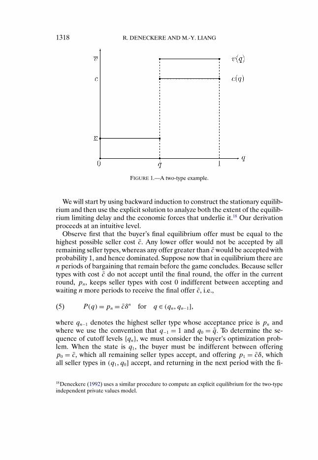
where c̄ > 0, v > 0� v̄ > c̄, and v̄ ≥ v (see Figure 1). As noted above, when thebuyer’s valuation function v(·) is constant, we obtain the private values modelas a special case. In the present example, this translates to the condition thatv= v̄.
17The triplet {P(·)�R(·)� t(·)} also describes the equilibrium continuation following nonequilib-rium buyer offers p: All seller types whose reservation price falls below p accept and all othertypes reject. If q is the induced state and the offer satisfies the equation p= P(q), then followingrejection, the buyer raises her offer to P(t(q)). If p is not in the range of the function P(·), sothat we have p > P(q), then following rejection of p, the buyer randomizes between the mini-mum and maximum elements of P(Υ(q)) so as to rationalize type q’s acceptance of the previousoffer p. Note that the latter type of offer will never arise along the equilibrium path, because thebuyer could have lowered her offer to P(q) and still have induced the same acceptances.
1318 R. DENECKERE AND M.-Y. LIANG
FIGURE 1.—A two-type example.
We will start by using backward induction to construct the stationary equilib-rium and then use the explicit solution to analyze both the extent of the equilib-rium limiting delay and the economic forces that underlie it.18 Our derivationproceeds at an intuitive level.
Observe first that the buyer’s final equilibrium offer must be equal to thehighest possible seller cost c̄. Any lower offer would not be accepted by allremaining seller types, whereas any offer greater than c̄ would be accepted withprobability 1, and hence dominated. Suppose now that in equilibrium there aren periods of bargaining that remain before the game concludes. Because sellertypes with cost c̄ do not accept until the final round, the offer in the currentround, pn, keeps seller types with cost 0 indifferent between accepting andwaiting n more periods to receive the final offer c̄, i.e.,
P(q)= pn = c̄δn for q ∈ (qn�qn−1]�(5)
where qn−1 denotes the highest seller type whose acceptance price is pn andwhere we use the convention that q−1 = 1 and q0 = q̂. To determine the se-quence of cutoff levels {qn}, we must consider the buyer’s optimization prob-lem. When the state is q1, the buyer must be indifferent between offeringp0 = c̄, which all remaining seller types accept, and offering p1 = c̄δ, whichall seller types in (q1� q0] accept, and returning in the next period with the fi-
18Deneckere (1992) uses a similar procedure to compute an explicit equilibrium for the two-typeindependent private values model.
BARGAINING WITH INTERDEPENDENT VALUES 1319
nal offer p0. Letting mn = qn−1 − qn denote the period n ex ante probability ofagreement, we therefore have
R(q1)= (v− δc̄)m1 + δ(v̄− c̄)m0 = (v− c̄)m1 + (v̄− c̄)m0�
where m0 = (1 − q̂)� Solving this equation for m1 yields m1 = (v̄− c̄)m0/c̄.Similarly, when n > 1� at state qn the buyer must be indifferent between
making the offer pn, which will be accepted by all seller types in (qn�qn−1], andmaking the next higher offer pn−1, which will be accepted by all seller types in(qn�qn−2]:
R(qn)= (v−pn)mn + δR(qn−1)(6)
= (v−pn−1)mn +R(qn−1)�(7)
Combining (6) and (7), we obtain
(1 − δ)R(qn−1)= (pn−1 −pn)mn�(8)
Equation (8) has the following interpretation. The advantage to making theoffer pn−1 rather than the offer pn is that the buyer gets to collect her con-tinuation surplus R(qn−1) one period earlier. At the same time, she losespn−1 − pn = (1 − δ)pn−1 on the customers in (qn�qn−1]. By construction, thegains from accelerating trade must balance out the losses.
Since the price decrease from period n−1 to period n is equal to (1−δ)pn−1,we may rewrite (8) as
R(qn−1)= pn−1mn�(9)
Equation (9) has the interesting interpretation that the buyer’s expected pay-ment in period n must be equal to her discounted expected continuation sur-plus, i.e., pnmn = δR(qn−1). It therefore follows from (7) that in each periodn > 1, the buyer’s expected total surplus is equal to the expected social surplusgenerated in that period:
R(qn)= vmn�(10)
Finally, substituting (10) into (8) converts the “no net gains from acceleratingtrade” condition into a difference equation in mn:
mn = v
c̄δn−1mn−1�(11)
Defining ρ= v/c̄, we may solve this difference equation by forward recursion,using the boundary condition m1 = (v̄− c̄)m0/c̄:
mn = ρn−1δ−(n(n−1))/2m1 = ρn−1δ−(n(n−1))/2 (v̄− c̄)m0
c̄�(12)
1320 R. DENECKERE AND M.-Y. LIANG
Let us write mn(δ) to denote explicitly the dependence of the solution in (12)on δ and letN(δ)= min{n :
∑n
i=0mi(δ)≥ 1}. For simplicity, assume that we arein the generic case where
∑n
i=0mi(δ) > 1. We may then summarize the solutionas follows:
PROPOSITION 1: Let v(·) and c(·) be given by (4), let 0< qN−1 < · · ·< q0 = q̂be defined recursively by (11), and let pn be defined by (5). Then for all δ < 1 theunique stationary triplet is given by
P(q)= pn� q ∈{ [0� qn−1]� if n=N ,(qn�qn−1]� if n= 0�1� � � � �N − 1;
t(q)= qn−2� q ∈{ [0� qn−1]� if n=N ,(qn�qn−1]� if n= 2�3� � � � �N − 1,(q1�1]� if n= 1;
R(q)=∫ qn−1
q
(v(z)−pn−1)dz+ δR(qn−2)�
q ∈{ [0� qN−1]� if n=N ,(qn�qn−1]� if n= 2�3� � � � �N − 1,(qn�1]� if n= 1.
According to Proposition 1, the buyer starts out by offering pN−1, which allseller types in [0� qN−2] accept. Upon rejection, the buyer raises her offer topN−2, which is accepted by all seller types in (qN−2� qN−3], and so on until thestate q0 is reached, at which point the seller makes her final offer p0 = c̄. Bar-gaining therefore lasts for N(δ) periods.19
We are interested in the behavior of the above solution as δ converges to 1.To gain some insight, let us first consider the case where ρ ≥ 1. Note that thiscase includes the private values model, where ρ= v/c̄ > 1. The economic sig-nificance of the inequality ρ≥ 1 is that it implies v > c̄δn = pn for all n≥ 1, sothat at any point in the game the buyer always expects to earn a positive surplusif her offer pn is accepted. As we work backward from the terminal state, thebuyer’s expected discounted surplus therefore grows, i.e., R(qn)−R(qn−1) > 0.Because the buyer trades off gains from increased price discrimination againstdelayed receipt of the continuation value, she will become more reluctant toprice discriminate as n increases. Thus, the acceptance probability is higher inearlier stages of the bargaining process; formally this is reflected in the factthatmn >mn−1 for all n > 1. Note that this inequality immediately implies thatthe number of bargaining rounds N(δ) is finite and uniformly bounded in δ.20
19In the nongeneric case where∑N
i=1mi(δ) = 1, the buyer may randomize between the initialoffers pN and pN−1, so that bargaining can last for one additional period.20Indeed, m1 = (v̄− c̄)(1 − q̂)/c̄ does not depend on δ.
BARGAINING WITH INTERDEPENDENT VALUES 1321
It follows that the Coase conjecture holds, because if bargaining can last for atmost N̂ rounds (where N̂ is the uniform bound onN(δ)), the initial price is nolower than δN̂−1c̄ and hence converges to c̄ as δ→ 1. We conclude that whenρ≥ 1, the solution behaves qualitatively exactly like in the private values case.
When ρ < 1, however, the equilibrium takes on a different character fromthe private values case. Indeed, with ρ < 1, it is always the case that when δ issufficiently close to 1 there exists an initial range of integers n ≥ 1 for whichv < c̄δn. For such n the buyer expects to earn a negative surplus when the selleraccepts her offer pn. Working backward from the state q0, the buyer’s expectedprofits are decreasing in n as long as the inequality v < c̄δn−1 continues to hold.Because the buyer trades off gains from increased price discrimination againstdelayed receipt of the continuation value, she will therefore become more ea-ger to price discriminate as n increases. Formally, this is reflected in the factthat the ex ante acceptance probability mn is decreasing in n. Importantly, ob-serve that when δ approaches 1, the number of time periods over which theinequality v < c̄δn−1 holds increases without bound as the discount factor ap-proaches 1. Consequently, unlike in the private values case, real delay mayoccur, even in the limit, as bargaining frictions are allowed to vanish.
To determine whether real delay occurs, let us calculate how far the back-ward construction can be extended in the limit as δ → 1� i.e., let q∗ =1 − ∑∞
i=0mi(1) = 1 − m0 − m1(1 + ρ + ρ2 + · · ·). If q∗ < 0,21 we can defineN̂ = min{n :
∑n
i=0mi(1) ≥ 1}. Bargaining then lasts no more than N̂ periods,regardless of the discount factor δ. As observed above, the Coase conjecturethen holds. This is true despite the fact that when ρ < 1, then for large δ theacceptance probability mn is decreasing in n (1< n ≤ N̂). If q∗ = 0, the num-ber of bargaining rounds is finite for any δ < 1, but increases without boundas δ→ 1. Nevertheless, as Proposition 2 shows, the Coase conjecture holds forthis case as well. Some simple computations show that the condition q∗ ≤ 0 isequivalent to the condition E(v)≥ c̄.22 We conclude that in the two-type modelthe Coase conjecture holds if and only if the static incentive constraints permitan efficient outcome (see Lemma 1).
When q∗ > 0, then in the limit the backward construction “gets stuck” at thequantity q∗. The reason for this is straightforward. By the definition of q∗, forany q > q∗ there exists an n <∞ such that for all δ < 1 we have
∑n
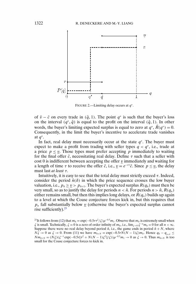
i=0mi(δ)≥1 − q. For any such state, it will take no more than n periods before the buyermakes her final offer, independently of the discount factor δ. Thus for any stateq > q∗, the Coase conjecture applies, yielding the buyer a limiting expectedsurplus R̃(q)=E[v(z)− c̄|z ≥ q]. Now consider Figure 2: The buyer makes anexpected loss of c̄ − v on every trade in (q∗� q̂) and makes an expected gain
21Note that when ρ≥ 1, we have q∗ = −∞, so that in this case the inequality q∗ < 0 always holds.22Indeed, for ρ < 1 we have
∑∞i=0mi(1)=m0(1 + (v̄− c̄))/(c̄(1 − ρ))= (1 − q̂)(v̄− v)/(c̄ − v).
The inequality q∗ ≤ 0 is therefore equivalent to the condition E(v)= vq̂+ v̄(1 − q̂)≥ c̄.
1322 R. DENECKERE AND M.-Y. LIANG
FIGURE 2.—Limiting delay occurs at q∗.
of v̄ − c̄ on every trade in (q̂�1). The point q∗ is such that the buyer’s losson the interval (q∗� q̂) is equal to the profit on the interval (q̂�1). In otherwords, the buyer’s limiting expected surplus is equal to zero at q∗, R̃(q∗)= 0.Consequently, in the limit the buyer’s incentive to accelerate trade vanishesat q∗.
In fact, real delay must necessarily occur at the state q∗. The buyer mustexpect to make a profit from trading with seller types q < q∗, i.e., trade ata price p ≤ v. Those types must prefer accepting p immediately to waitingfor the final offer c̄, necessitating real delay. Define τ such that a seller withcost 0 is indifferent between accepting the offer v immediately and waiting fora length of time τ to receive the offer c̄, i.e., v = e−rτc̄. Since p ≤ v, the delaymust last at least τ.
Intuitively, it is easy to see that the total delay must strictly exceed τ. Indeed,consider the period n̂(δ) in which the price sequence crosses the low buyervaluation, i.e., pn̂ ≥ v > pn̂+1. The buyer’s expected surplus R(qn̂)must then bevery small, so as to justify the delay for periods n < n̂. For periods n > n̂, R(qn)either remains small, but then this implies long delays, orR(qn) builds up againto a level at which the Coase conjecture forces kick in, but this requires thatpn fall substantially below v (otherwise the buyer’s expected surplus cannotrise sufficiently).23
23It follows from (12) thatmn̂ = exp(−0�5rτ2/ζ)ρ−0�5m1. Observe thatmn̂ is extremely small whenζ is small. Technically, ζ = 0 is a zero of order infinity of mn̂, i.e., limζ→0 ζ
−nmn̂ = 0 for all n <∞.Suppose there were no real delay beyond period n̂, i.e., the game ends in period n̂+N , whereNζ → 0 as ζ → 0. From (11) we have mn̂+N = exp(−0�5rN(N − 1)ζ)mn̂. Hence qn̂ − q
n̂+N ≤Nmn̂+N = (Nζ)(ζ−1 exp(−0�5r[τ2 + N(N − 1)ζ2]/ζ))ρ−0�5m1 → 0 as ζ → 0. Thus mn̂+N is toosmall for the Coase conjecture forces to kick in.
BARGAINING WITH INTERDEPENDENT VALUES 1323
One of the main breakthroughs in this paper is to figure out exactly howmuch delay there must be at the state q∗. Proposition 2 shows that the limit-ing delay actually must last twice as long, i.e., must be equal to 2τ. The reasonfor the doubling of τ is the symmetry of the solution around the period n̂(δ).To see the reason for this symmetry, let us for simplicity assume that pn̂ = v,so that the buyer’s expected surplus from having her period n̂ offer acceptedis equal to zero. It then follows from (9) and (10) that the percentage growthin the buyer’s expected surplus equals the percentage growth in price.24 Notethat the percentage price increase is the same in every period. Consequentlythe buyer’s expected surplus grows symmetrically around the period n̂, i.e.,Rn̂+k+1 =Rn̂−k. It follows from (10) that acceptance probabilities are also sym-metric around period n̂, i.e.,mn̂+k+1 =mn̂−k. We conclude that for any δ it takesas much time to go from qn̂ − ε to qn̂ as it does to go from qn̂ to qn̂ + ε. Ob-serve that limδ→1 qn̂ = q∗,25 so that in the limit it takes twice as long to travelfrom q∗ − ε to q∗ + ε as from q∗ to q∗ + ε. Because there is no limiting delaybetween q∗ + ε and q = 1, we conclude that the limiting real delay betweenq∗ − ε and 1 must equal 2τ.
To complete the description of the limiting outcome when q∗ > 0, observethat for q < q∗ − ε the buyer’s limiting continuation surplus is strictly positive(by offering the acceptance price of type q∗ − ε, in the limit the buyer earnsat least (v − ρ2c̄)(q∗ − ε)). As a consequence, the buyer has an incentive toaccelerate trade and the Coase conjecture again applies: for any ε > 0 thereexists n <∞ such that, regardless of the discount factor, it takes no more thann steps for the buyer to trade with type q. In the limit, there is therefore nodelay between 0 and q∗ − ε. Because ε is arbitrary, all limiting delay thereforeoccurs at q∗ and all types in [0� q∗) trade at the common pricep∗ = e−2rτc̄ = ρ2c̄.To summarize, we have:
PROPOSITION 2: The Coase conjecture obtains if and only if E(v) ≥ c̄� Letq∗ = (c̄ −E(v))/(c̄ − v) and ρ= v/c̄. Then when E(v) < c̄, as δ converges to 1,all seller types in [0� q∗) trade immediately at the price p∗ = c̄ρ2 and all types in(q∗�1] trade at the price c̄ after a delay of length T discounted such that e−rT = ρ2.
The two-type example teaches us that it is the possibility of ex post buyerregret (i.e., the buyer’s expectation to earn a negative surplus should her of-fer be accepted) that slows down the bargaining. This slowdown may or maynot be sufficiently strong to produce limiting delay. Whether the Coase con-jecture holds, and thus whether there is no limiting delay, depends on whether
24More precisely, (Rn̂+k+1 − Rn̂+k)/Rn̂+k = (v − pn̂+k)/pn̂+k and (Rn̂−k − Rn̂−k+1)/Rn̂−k+1 =(pn̂−k − v)/v for all k≥ 1.25Because the acceptance price of qn̂ is v, we must have qn̂ ≤ q∗. However, if limδ→1 qn̂ were lessthan q∗, then by the definition of q∗ the buyer would earn negative expected surplus, a contradic-tion.
1324 R. DENECKERE AND M.-Y. LIANG
the condition E(v)≥ c(1) is satisfied. If so, the buyer’s expected continuationsurplus remains bounded away from zero for all states q > 0, so the incentiveto speed up receipt of this continuation value dominates the buyer’s incentiveto price discriminate. When E(v) < c(1), the Coase conjecture forces still op-erate at all values of the state where the buyer’s expected continuation valueremains bounded away from zero. However, there exists a state q∗ for whichthe limiting continuation value converges to zero. Near this state, the incentiveto price discriminate remains strong as the discount factor converges to 1, al-lowing real delay to occur. As a consequence, when δ is near 1, the bargainingoutcome is characterized by two short time periods during which there is a highprobability of agreement, interspersed with a long period of delay in which theprobability of agreement is negligible. The length of the delay is increasing in c̄and decreasing in v, but does not depend on v̄.
We conclude this section by investigating the efficiency properties of thelimiting bargaining mechanism characterized in Proposition 2. WheneverE(v)≥ c̄, the Coase conjecture leads to first-best efficiency. However, whenE(v) < c̄ (so that first-best efficiency is no longer possible), the Coase conjec-ture forces operate in a way so as to cause excess delay. To see this, note thatall seller types in the interval [0� q̂] have the same valuation, so the ex ante op-timal allocation requires that their allocation be undistorted. However, in thelimiting bargaining outcome, only types q in the interval [0� q∗
1] trade at timezero; the remainder must trade after a delay of length T . In particular, socialwelfare can be increased by having all types q ∈ (q∗
1� q̂] trade at time zero at theprice c̄e−rT instead. Indeed, all such seller types are indifferent between thesetwo options and the buyer pays the same discounted price, but gets to tradeearlier.26
In Section 5, we show that many of the qualitative properties of the limitingbargaining outcome do not depend on there being just two types. Although ingeneral there might be more than one location in which there is limiting delay,the Coase conjecture forces continue to operate at any state q for which thebuyer’s limiting expected surplus is not zero. We also show that, as in the two-type case, there is limiting delay at any state q∗
n for which the buyer’s limitingexpected surplus is zero and that the length of this delay does not depend onthe global structure of the cost and valuation functions. In Section 6, we showthat the limiting bargaining outcome generically exhibits excess delay when-ever E(v) < c(1) and we relate the size of the efficiency loss to the size of theequilibrium delay.
26In the resulting mechanism, the buyer will enjoy strictly positive expected surplus; this meanswe can increase the probability of trade on the interval (q̂�1] above ρ2, thereby further increasingwelfare. We can maintain incentive compatibility by raising the price paid by seller types in [0� q̂]in such a way as to keep them indifferent between the two options. The ex ante optimal mech-anism obtains when the probability of trade over the interval [0� q̂] cannot be raised any furtherwithout making the buyer sustain losses.
BARGAINING WITH INTERDEPENDENT VALUES 1325
4. EXISTENCE AND UNIQUENESS
For the special case of private values, Gul, Sonnenschein, and Wilson (1986)demonstrate that there exists a unique stationary triplet and that all sequentialequilibrium outcomes are the outcomes of some stationary equilibrium, pro-vided that Assumption 1 holds and the seller’s cost function satisfies a Lipschitzcondition at q= 1:
ASSUMPTION 2: There exists L<∞ such that c(1)− c(q)≤L(1 −q) for allq ∈ [0�1].
Theorem 1 generalizes the Gul, Sonnenschein, and Wilson result to the caseof interdependent values. The key step in establishing uniqueness of the sta-tionary triplet is to show that there exists a critical value of the state q1 < 1,such that in any sequential equilibrium, whenever the state exceeds q1, thebuyer must make an offer that all remaining seller types will accept (see Lem-mas A-1 and A-4 in Appendix A). This uniquely pins down a stationary triplet(R� t�P) on the interval (q1�1]. We then use backward induction on the state,employing the functional equations (2) and (3) to successively uniquely extendthe triplet (R� t�P) to the entire interval [0�1]. One difficulty our proof mustovercome is that the size of the extension from any state q is proportional tothe buyer’s expected surplus R(q). In the private values case, R(q) is decreas-ing in q, so that the size of the extension increases as we move back from theterminal state; this allows the extension process to terminate in a finite num-ber of steps.27 When valuations are positively related, however, R(q) may beincreasing in q over some interval, so it is quite conceivable that the extensionprocedure might never terminate.28
To overcome this difficulty, we first construct a stationary triplet whose equi-librium surplus coincides withR(q) and with the property thatR(q) is boundedaway from zero over the interval [0� q1]. To establish that the extension pro-cedure in the construction of this triplet does not get stuck before the statereaches zero, we select each extension step to be maximal, in that its lengthcoincides with a bargaining period. More precisely, there is a decreasing se-quence of cutoff levels {qn} with the property that for each n > 1 there existsno state less than qn+1 for which the buyer selects an offer acceptable to sellertypes in (qn�1]. We also make essential use of the maximality of this extensionin the proof of our characterization theorem in Section 5 (Theorem 3).
27For a precise argument in the private values case, see, e.g., Ausubel and Deneckere (1989a,Lemma 2).28Vincent (1989, Theorem 1) adapts Gul, Sonnenschein, and Wilson’s (1986) arguments to estab-lish existence under Assumptions 1 and 2, but his proof fails to demonstrate that the extensiondoes not get stuck at some state q > 0. Our proof also dispenses with Vincent’s requirement thatv(·) be nondecreasing.
1326 R. DENECKERE AND M.-Y. LIANG
THEOREM 1: Suppose that Assumptions 1 and 2 hold. Then for any δ < 1,there exists a unique stationary triplet (R(·)� t(·)�P(·)) on [0�1] and every sequen-tial equilibrium outcome is the outcome of some stationary equilibrium. Further-more, there exists N(δ) <∞ such that bargaining concludes with probability 1 inN(δ) periods.
Although Theorem 1 guarantees that bargaining will end in a finite num-ber of periods, there is a big difference with the private values case. Whenvalues are private, the number of bargaining rounds remains bounded aboveas the discount factor approaches 1 (see Deneckere (1992)). With interde-pendent values, this property cannot generally hold. Otherwise, the Coaseconjecture would always apply, but according to Lemma 1 this is impossiblewhenever E(v(q)) < c(1). Under the latter assumption, the number of bar-gaining rounds must necessarily increase without bound as the discount factorapproaches 1.
Our second result establishes the existence of stationary equilibrium underextremely weak conditions. We drop Assumption 2 and replace Assumption 1with the much weaker condition:
ASSUMPTION 3: For every q ∈ [0�1], v(q)≥ c(q).
Our technique of proof consists of approximating v(·) and c(·) by functionsthat satisfy Assumptions 1 and 2, and arguing that an appropriate chosen limitof the stationary equilibria of the approximating games is a stationary equi-librium of the limit game. This generalizes Ausubel and Deneckere (1989a,Theorem 4.2) to the case of interdependent values.
THEOREM 2: Suppose Assumption 3 holds. Then there exists a stationary equi-librium.
Theorem 2 is of interest, because it covers the “no gap” case, where v(1)=c(1) but v(q) > c(q) for all q < 1. Using this stationary equilibrium, it is possi-ble to mimic the construction in Ausubel and Deneckere (1989a, Theorem 6.4)to generate a rich class of equilibria that yield arbitrarily long periods of delay(dissipating an arbitrarily large fraction of the surplus). Theorem 2 also coversthe interesting case in which v(0)= c(0) but v(q) > c(q) for all q > 0.29
29However, as shown by Akerlof (1970), under some conditions the stationary equilibrium maythen involve infinite delay at q = 0 (in the terminology of Section 5, this happens wheneverK = ∞). Furthermore, when v(q̃) = c(q̃) for some 0 < q̃ < 1, the stationary equilibrium mayinvolve infinite delay at q̃. For example, this happens whenever q̃= q∗
1 , c′−(q
∗1)= ∞, and δ= 0.
BARGAINING WITH INTERDEPENDENT VALUES 1327
5. CHARACTERIZING THE LIMITING EQUILIBRIUM PATH
In this section, we will use the results of Section 4 to characterize the limitingdelay whenever the buyer’s and seller’s valuation functions are neoclassical,30
i.e., satisfy:
ASSUMPTION 4: The functions v(·) and c(·) are step functions, each havingat most a finite number of steps.
We will show that in the limit the seller’s acceptance function becomes a stepfunction, taking on the K distinct values p∗
K−1� � � � �p∗0, where p∗
K−1 < p∗K−2 <· · · < p∗
1 < p∗0 = c(1). As a consequence, in the limit the buyer makes only
K serious equilibrium offers. More precisely, the buyer starts by making theoffer p∗
K−1, which is accepted with probability q∗K−1. The state q∗
K−1 is such thatthe buyer’s limiting expected surplus upon rejection of the offer p∗
K−1 equalszero. As a consequence, the buyer does not have any incentive to acceleratetrade when the state is q∗
K−1. In fact, Theorem 3 asserts that there is real delay,of length TK−1, until the buyer makes her next serious offer, p∗
K−2. The offerp∗K−2 is accepted with probability q∗
K−2 − q∗K−1, where the state q∗
K−2 is againsuch that the buyer’s expected limiting surplus at q∗
K−2 equals zero. The lack ofan incentive to accelerate trade at q∗
K−2 leads to a delay of length TK−2, uponwhich the buyer makes her next serious offer, p∗
K−3, which is accepted withprobability q∗
K−3 − q∗K−2. This process continues in a similar fashion until the
state reaches q∗1, where, after a delay of length T1, the buyer makes her final
offer p∗0 = c(1), which the seller accepts.
The qualitative implications of Theorem 3 for δ near 1 are as follows. Inequilibrium the game starts out with a small length of real time over which thebuyer makes serious offers near p∗
K−1 that cumulatively have a significant like-lihood of acceptance (roughly equal to q∗
K−1). This is followed by an “impasse,”i.e., a period of length roughly equal to TK−1 over which the buyer raises heroffer gradually from the level p∗
K−1 to the next level p∗K−2. The offers are all se-
rious, but cumulatively have a very small likelihood of acceptance (convergingto zero as δ converges to 1). This is followed by a small period over which thebuyer’s offers hover around p∗
K−2, which cumulatively have acceptance prob-ability close to q∗
K−2 − q∗K−1. The sequence of periods of high probability of
acceptance of offers near p∗n followed by impasses of length roughly equal
to Tn (n = K − 1� � � � �1) continues until the buyer’s offer starts approachingp∗
0 = c(1), upon which agreement is quickly reached.Formally, let us set q∗
0 = 1 and p∗0 = c(1), and iteratively define q∗
n and p∗n as
q∗n = max
{q ∈ [0� q∗
n−1) :∫ q∗
n−1
q
(v(z)−p∗n−1)dz ≤ 0
}�(13)
30Note that arbitrary valuation functions can be arbitrarily closely approximated by neoclassicalones.
1328 R. DENECKERE AND M.-Y. LIANG
whenever the set on the right-hand side of (13) is nonempty and q∗n = 0 other-
wise, and
p∗n = c(q∗
n)+ (v(q∗n)− c(q∗
n))2
p∗n−1 − c(q∗
n)�(14)
ending the process whenever q∗n reaches 0. Note that Assumptions 1 and 4
guarantee that this happens in a finite number of steps. We denote this num-ber by K. For each n ∈ {1� � � � �K − 1} let us also define Tn as the solution toexp(−rTn)= ρ2
n, where
ρn = v(q∗n)− c(q∗
n)
p∗n−1 − c(q∗
n)�(15)
The intuition behind the construction of (13)–(15) is analogous to the intu-ition for the limiting solution in the two-step example in Section 3. Observethat for states q > q∗
1, the buyer’s expected continuation surplus is strictly posi-tive, because she can always make the offerp∗
0 = c(1), which would be acceptedby all seller types. For such states, the Coase conjecture forces thus cause herto accelerate trade and, in the limit, make the offer p∗
0 = c(1) instantaneously.As in the two-type case, over the interval (q∗
1�1] the seller’s acceptance func-tion and the buyer’s expected surplus converge to the limits P̃(q) = c(1) andR̃(q)= ∫ 1
q(v(z)−c(1))dz, respectively. At q= q∗
1, the buyer’s expected surplusis zero and real delay occurs. Analogously to the two-type case, seller type c(q∗
1)is indifferent between accepting the offer p∗
1 and waiting for a length of timeT1 to receive the final offer p∗
0 = c(1). Formula (14) says that exp(−rT1)= ρ21.
In other words, the solution dictates that T1 equal 2τ1, where τ1 is the length oftime that makes seller type c(q∗
1) indifferent between accepting the offer v(q∗1)
and waiting for the final offer p∗0 = c(1).
Over the interval (q∗2� q
∗1) the buyer’s expected limiting surplus is strictly pos-
itive, because she can always make the offer p∗1, which would be accepted by
all seller types q < q∗1. For states in the interval (q∗
2� q∗1), the Coase conjec-
ture forces again lead the buyer to accelerate trade and, in the limit, makethe offer p∗
1 immediately. Over this interval, the seller’s acceptance functionand the buyer’s expected surplus therefore respectively converge to the limitsP̃(q) = p∗
1 and R̃(q) = ∫ q∗1
q(v(z)− p∗
1)dz. At q∗2, the buyer’s expected surplus
is zero, and so on.To simplify the proofs, we make the following nondegeneracy assumption.31
31At the cost of some additional complexity in the proofs, we can show that Theorem 3 con-tinues to hold, even when Assumption 5 fails. This is because, for large δ, all but an arbitrar-ily small fraction of the delay happens in a left neighborhood of q∗
n. However, to cover thiscase, we need to slightly redefine q∗
n. To see why, note that when v(·) has a discontinuity at
BARGAINING WITH INTERDEPENDENT VALUES 1329
ASSUMPTION 5: The functions v(·) and c(·) are continuous at q∗n for all n ∈
{1� � � � �K}.Assumption 5 is not very onerous, because it holds generically given As-
sumptions 1 and 4. We may now state the following generalization of Proposi-tion 2:
THEOREM 3: Suppose Assumptions 1, 4, and 5 hold. Let q∗n�p
∗n, and Tn be
given by (13), (14), and (15), respectively. Then, in the limit, as δ→ 1, the seller’sacceptance function and the buyer’s surplus function converge to
P̃(q)= p∗n� q ∈
{ [0� q∗n]� if n=K − 1,
(q∗n+1� q
∗n]� if n= 0� � � � �K − 2;
R̃(q)=∫ q∗
n
q
(v(z)−p∗n)dz� q ∈
{ [0� q∗n]� if n=K − 1,
(q∗n+1� q
∗n]� if n= 0� � � � �K − 2.
Furthermore, in the limit, the buyer successively makes the serious offers p∗K−1� � � � �
p∗0, but for n=K− 1� � � � �1 delays trade for a length of time Tn between the offersp∗n and p∗
n−1 by making offers that are sure to be rejected.
The proof of Theorem 3 proceeds in three steps (see Appendix C). First,we consider the special case K = 1, for which the limiting outcome exhibitsno delay (see Corollary 1). Next, we treat the case K = 2, for which there is asingle bargaining impasse, and establish the length of the associated delay (seeCorollary 2). The proof for the case K > 2 then consists of a finite number ofrepetitions of the arguments for the case K = 2.
For the special case in which K = 1, i.e., q∗1 = 0, Theorem 3 says that the
seller’s limiting acceptance function has a single step, i.e., P̃(q) = p∗0 = c(1)
for all q ∈ [0�1]. Furthermore, the buyer’s limiting expected surplus satisfiesR̃(q) = ∫ 1
q[v(z) − c(1)]dz for all q ∈ [0�1]. Thus, in the limit, the seller ac-
cepts an offer if and only if it is greater than or equal to c(1), and from anyinitial state q ∈ [0�1], the buyer makes the offer c(1), which is sure to be ac-cepted. The case K = 1 (or q∗
1 = 0) therefore delineates the precise circum-stances under which the Coase conjecture does and does not hold. Note thatthe condition q∗
1 = 0 holds if and only if there exists no q ∈ [0�1] for which∫ 1q[v(z)− c(1)]dz < 0. We thus have the next statement:
COROLLARY 1: Suppose Assumptions 1, 4, and 5 hold. Then the Coase con-jecture holds if and only if E[v(z)− c(1)|z ≥ q] ≥ 0 for all q ∈ [0�1].
q∗n−1, we may have
∫ q∗n−1
q(v(z) − p∗
n−1)dz = 0 in a left neighborhood of q∗n−1, so q∗
n would beill defined. Furthermore, q∗
n then must be the left endpoint of this interval, i.e., q∗n = sup{q ∈
[0� q∗n−1) :
∫ q∗n−1
q(v(z)−p∗
n−1)dz < 0}.
1330 R. DENECKERE AND M.-Y. LIANG
When E[v(z) − c(1)|z ≥ q] > 0 for all q ∈ [0�1], the buyer’s limiting ex-pected surplus is strictly positive at every initial state, providing her withan incentive to accelerate trade. This case is analogous to the case of a“gap” when values are private. When there exists some q̃ ∈ [0�1) such thatE[v(z)− c(1)|z ≥ q̃] = 0 (but still E[v(z)− c(1)|z ≥ q] ≥ 0 for all q ∈ [0�1]),showing that there cannot be any delay at q̃ requires a more sophisticatedproof.
Observe that in the two-type case, whenever Assumption 1 holds, the condi-tion that E[v(z)− c(1)|z ≥ q] ≥ 0 for all q ∈ [0�1] is equivalent to the condi-tion E(v)≥ c(1). As a consequence, we were able to conclude that the Coaseconjecture held if and only if the static incentive constraints admit an efficientoutcome. In general, however, it is possible that E(v) ≥ c(1), but that thereexists some q ∈ (0�1) for which E[v(z)− c(1)|z ≥ q] < 0, so that q∗
1 > 0. Ournext example illustrates this possibility.
EXAMPLE: Modify the example from Section 3 as follows. Pick ε > 0 andc̄ > 0, and select c̄ and so that q∗
1 > ε. Now redefine v on [0� ε] so that v(q)= γand select γ sufficiently large that E(v)≥ c(1).
In the above example, it is feasible for the buyer to trade with all sellertypes at the single price c(1), but because q∗
1 > 0, the limiting bargaining out-come must exhibit real delay. For limiting delay to be absent, the conditionE(v)≥ c(1) therefore generally needs to be strengthened. One possibility is toassume that the function v(·) is nondecreasing. Then the conditionE(v)≥ c(1)becomes equivalent to the condition of Corollary 1, and hence is both neces-sary and sufficient for the absence of delay.
Now consider the case K = 2. Theorem 3 then asserts that the seller’s lim-iting acceptance function has two steps, i.e., P̃(q) = p∗
1 for q ∈ [0� q∗1] and
P̃(q) = c(1) for q ∈ (q∗1�1]. Clearly, the argument for the case K = 1 estab-
lishes that there cannot be any delay at any state q > q∗1, explaining the shape
of P̃ over this interval. The additional content of Theorem 3 therefore con-sists of tying down the length of the limiting delay at q∗
1 and showing that therecannot be any delay at any state q < q∗
1:
COROLLARY 2: Suppose that Assumptions 1, 4, and 5 hold, and suppose thatK = 2. Then as δ tends to 1 the acceptance price of any seller type q > q∗
1 convergesto c(1) and the acceptance price of any seller type q < q∗
1 converges to p∗1.
The proof of Corollary 2 is long and hard. The essential ideas are as follows.As in Corollary 1, the Coase conjecture ensures that there is no limiting delayfor any q > q∗
1. Note that this implies that the length of any limiting delay willnot depend on the detailed behavior of the cost or valuation function to theright of q∗
1. As in the two-type case, we also know that the price must drop fromthe level c(1) to below v(q∗
1), because otherwise the buyer would sustain losses
BARGAINING WITH INTERDEPENDENT VALUES 1331
on any seller type q < q∗1 without compensating gains when the state reaches q∗
1.Keeping seller type q∗
1 indifferent between c(1) and v(q∗1) requires a real delay
of length τ1, so the total delay must be at least this long. To establish that thetotal delay length is 2τ1 requires a symmetry argument analogous to the one inthe two-type case. Unfortunately, establishing this symmetry is rather involved.The reason for the complication is that when the cost function has multiplejumps to the right of q∗
1 the no net gains from accelerating trade condition nolonger need imply that the buyer’s current expected payment is equal to herdiscounted expected continuation surplus (see (8)). Since the latter propertylinks symmetry in price growth to symmetry in surplus growth, figuring out thelength of the limiting delay becomes very complicated.
The reason for the failure of (8) is that unlike in the two-type case, theseller’s acceptance function may not be flat on the interval (qn�qn−1], becauseof the presence of discontinuities in the cost schedule. As a consequence, itis no longer the case that for an arbitrary initial state, the buyer optimizes byselecting the endpoint of one of these intervals. Therefore, at an initial cutoffstate qn, the buyer may be indifferent between selecting the next cutoff levelqn−1 and some state q in the interior of the interval (qn−1� qn−2], rendering (8)invalid. To circumvent this difficulty, we establish that jumps in the acceptancefunction between two successive cutoff states can persist for at most an arbi-trarily small amount of real time when δ is sufficiently large. This implies thatthe solution becomes symmetric after an arbitrarily small amount of real time.
Our proof must overcome one additional potential problem. Note that atthe state qn1 at which a real time of length ε still has to pass before the pricereaches c(1), the buyer’s expected surplus is too small for the Coase conjectureforces to kick in and to produce no delay to the right of qn1 . Let period n2 belocated symmetrically to period n1, around the period n̂ in which the price levelreaches v(q∗
1), i.e., n̂= (n1 + n2)/2. Then at the state qn2 , the buyer’s expectedsurplus will also be insufficiently large for the Coase conjecture forces to kickin and to produce no delay to the left of qn2 . Thus, although symmetry of thesolution between qn2 and qn1 yields a delay that converges to 2(τ1 −ε), it is con-ceivable that there could be significant additional real delay to the left of qn2 ,because the buyer’s surplus there is insufficiently large. To show that this can-not happen, our proof establishes that during the time interval of length ε overwhich (8) does not yet apply, there exists a uniform upper bound J, indepen-dent of the discount factor δ, to the ratio between the acceptance probabilitygiven by the analogue to (11) and the true equilibrium acceptance probability.Using symmetry, this implies that it takes at most real time Jε for surplus togrow from its level at qn2 to a level sufficiently high for the Coase conjectureforces to kick in. Thus the total delay is at most Jε + 2(τ1 − ε)+ ε; becauseε can be taken arbitrarily small as δ approaches 1, and because qn1 and qn2
converge to q∗1, this yields the desired result.
1332 R. DENECKERE AND M.-Y. LIANG
6. THE INEFFICIENCY OF SEQUENTIAL BARGAINING
In this section, we evaluate the level of welfare achieved in the bargainingmechanism associated with the limiting equilibrium outcome of the dynamicbargaining game. In particular, we establish that this bargaining mechanism isex ante efficient if and only if the conditions of Corollary 1 hold, i.e., q∗
1 = 0.Intuitively, the reason why the dynamic bargaining mechanism may fail to max-imize the expected gains from trade over all incentive compatible and individ-ually rational mechanisms is that sequential equilibrium imposes additionaldynamic incentive constraints for the players. In particular, as we saw above,the Coase conjecture forces require that when the state is such that the buyer’slimiting expected continuation surplus is strictly positive, trade occurs imme-diately at the price c(1). In the case of independent valuations, and more gen-erally when interdependencies in valuations are sufficiently weak that q∗
1 = 0,these dynamic incentive constraints do not further restrict the set of feasiblemechanisms. However, as we will now show, when q∗
1 > 0, the same Coase con-jecture forces are at odds with efficiency.
To see this, observe that generically the ex ante efficient mechanism is uniqueand, when q∗
1 > 0, consists of either a three-step mechanism (in which the prob-ability of trade function χ(·) takes on three values, χ = 1�χ= λ ∈ (0�1), andχ= 0) or a two-step mechanism (in which χ(·) takes on two values, χ= 1 andχ = λ ∈ (0�1)).32 Intuitively, a three-step mechanism is optimal whenever itpays to exclude high cost seller types from the market (this happens wheneverthe surplus is small for a final segment of seller types and when their cost is highrelative to types with a lower index). Three-step mechanisms are clearly incon-sistent with the Coase conjecture forces, because in our game the buyer cannotcommit not to trade (with the high cost seller types). Furthermore, whenevertwo-step mechanisms are optimal, the limiting bargaining outcome will fail tobe efficient unless q∗
1 = qo (where qo is the cutoff level for χ in the two-stepmechanism). Below, we show that under Assumptions 1, 4, and 5 we neces-sarily have q∗
1 �= qo. Since the Coase conjecture forces determine the positionof q∗
1, it is fair to say that these forces are generally inconsistent with optimal-ity.33
Suppose that q∗1 > 0. Buyer individual rationality (in conjunction with Coase
conjecture forces) requires there to be delay at q∗1, i.e., seller types to the left
of q∗1 (including type q∗
1) trade earlier than seller types to the right of q∗1. Mean-
while ex ante optimality dictates that all sellers with the same cost type tradeat the same time. Because Assumptions 4 and 5 guarantee that there exists
32Myerson (1985) and Samuelson (1984) prove that the ex ante optimum can always be achievedby a two- or three-step mechanism. The argument that generically optimal mechanisms must beof this form is more involved.33In the nongeneric case where Assumption 5 is violated and c(·) is discontinuous at q∗
1 , it ispossible to have q∗
1 = qo.
BARGAINING WITH INTERDEPENDENT VALUES 1333
ε > 0 such that c(q∗1 + ε) = c(q∗
1), we necessarily have qo �= q∗1.34 Hence we
have shown the following assertion:
THEOREM 4: Suppose Assumptions 1, 4, and 5 hold, and suppose that q∗1 > 0.
Then the limiting bargaining outcome is not ex ante efficient, i.e., there exists anincentive compatible and individually rational mechanism that yields higher ex-pected gains from trade.
Theorem 4 says that whenever E(v) < c(1), and more generally wheneverq∗
1 > 0, there exist feasible mechanisms that yield higher welfare than in thefrictionless bargaining outcome of our model. Theorem 4 does not inform usabout the magnitude of the efficiency loss. In general, it is not possible to relyon the Coase conjecture forces alone to measure the size of this loss.35 Indeed,even when q∗
1 = qo and K = 2, the limiting mechanism can be very inefficient,because it exhibits excessive delay at q∗
1.36 Delay can be decreased by raisingthe initial price, but this lowers the buyer’s expected surplus. Indeed, the opti-mal mechanism obtains when the buyer’s expected surplus is zero. Thus R̃(0)provides a measure of excess delay.
Note that generically R̃(0) > 0. We will now argue that whenever this con-dition holds, reducing delay yields a nonnegligible welfare improvement.37
Indeed, suppose that 0 = q∗K < q
∗K−1 < · · · < q∗
1 < q∗0 = 1 and K ≥ 1. Since∫ q∗
K−10 (v(z) − p∗
K−1)dz = R̃(0) > 0� we can find a price p′ > p∗K−1 such that∫ q∗
K−10 (v(z)−p′)dz = 0. Now consider an alternative mechanism with the same
limiting offers and delays, except the very first ones. Let p′ be the initial priceoffered to seller types in [0� q∗
K−1], and let the delay between p′ and p∗K−2 be
T ′K−1 = r−1(ln(p∗
K−2 −c(q∗K−1))− ln(p′ −c(q∗
K−1))). Since T ′K−1 < TK−1, all seller
types in (q∗K−1�1] get to trade earlier after this alteration.
When values are strongly interdependent, the limiting bargaining outcomeneed no longer be second best, so many of the lessons we have learned fromthe private values model may be overturned. As an example of this, we demon-
34More concretely, we can improve welfare by having all seller types in the interval (q∗1� q
∗1 + ε)
trade at the price p∗1 at the same time as type q∗
1 . Incentive compatibility is maintained, becauseeach of these seller types is indifferent between this option and trading after a delay of length T1
at a price p∗0 = c(1). Furthermore, the buyer’s expected surplus increases because she pays the
same discounted price but gets to trade earlier, so buyer IR is still satisfied after the modification.35The Coase conjecture forces sometimes produce a large inefficiency (e.g., when the optimalmechanism has three steps or when q∗
1 is not near the endpoint of the interval on which c(·) isconstant).36What determines delay in the limiting mechanism is not the Coase conjecture forces, but ratherwhat happens when these forces vanish.37In the nongeneric case where R̃(0)= 0, it is possible for the limiting mechanism to be ex anteoptimal. However, this requires that K = 2 and q∗
1 = qo. The latter condition is, in turn, highlynongeneric.
1334 R. DENECKERE AND M.-Y. LIANG
strate below that the relative performance of different bargaining institutionsdepends significantly on the degree to which valuations are interdependent.
Ever since Coase’s (1972) famous paper, a central tenet of bargaining theoryhas been that a player’s inability to commit to walking away from the bargain-ing table may not only seriously undermine her bargaining power, but may alsoenhance the efficiency of the bargaining outcome. In other words, the welfaredistortions are lower when the uninformed party lacks commitment power thanwhen she has perfect commitment power. We claim that when values are inter-dependent, this conclusion may be reversed. To see this, let us again considerthe two-type example studied in Section 3 and let us assume that the fraction ofhigh cost seller types is sufficiently small that q∗
1 > 0, i.e., q̂ > (v̄− c̄)/(v̄− v).Among all incentive compatible mechanisms, the one most preferred by thebuyer is the one in which she gets to make a single take-it-or-leave-it offer (seeSamuelson (1984)). Because there are relatively few high cost seller types, thebuyer’s optimal take-it-or-leave-it offer is equal to zero. Under perfect com-mitment power, social welfare therefore coincides with the buyer’s expectedsurplus, i.e., equals vq̂. At the same time, the limiting bargaining outcomefrom Section 3 has trade occur immediately with seller types in [0� q∗
1] and withdelay discounted to ρ2 with seller types in (q∗
1�1]. Welfare therefore equalsvq∗
1 + ρ2[v(q̂ − q∗1) + (v̄ − c̄)(1 − q̂)] = vq̂ − ρ(v̄ − c̄)(1 − q̂) < vq̂, i.e., wel-
fare in the absence of commitment power falls short of welfare under perfectcommitment! Intuitively, this can happen because, with relatively few high val-uation types, the inefficiencies associated with ordinary monopsony power aresmaller than the inefficiencies caused by sequential bargaining.
7. FINAL REMARKS
We end the paper with two remarks. First, our characterization of limitingdelay has so far assumed that the valuation function v(·) and the cost func-tion c(·) are step functions with a finite number of steps. From an economicviewpoint, this covers all interesting cases, because in practice it would be veryhard to distinguish between arbitrary valuation and cost functions, and stepfunctions with a large but finite number of steps that approximate them arbi-trarily closely.
Nevertheless, it is interesting to inquire whether (13), (14), and (15) continueto characterize limiting delay when c(·) and v(·) are continuous functions. Oneway to answer this question is to see whether the proof of Theorem 3 can bemodified to allow for cases where c(·) and v(·) have a nonzero slope in thevicinity of q∗
n.38 Our method of calculating limiting delay there depends on
the property that when the state is qn, the buyer is indifferent between makingthe offer pn = P(qn−1), thereby leading all seller types in the interval (qn�qn−1]38Recall that the formulas for the limiting delay do not depend on the behavior of the functionsc(·) and v(·) other than in a neighborhood around q∗
n.
BARGAINING WITH INTERDEPENDENT VALUES 1335
to accept, and making the next higher offer pn−1 = P(qn−2), thereby leading allseller types in the interval (qn�qn−2] to accept.39 This property holds when v(·)and c(·) are linear, but is very hard to establish in general.
Fortunately, there is a much easier way to establish that the limiting delay ischaracterized by (13)–(15). We merely define the delay for the model with valu-ation function v(·) and the cost function c(·) to be the limit of the delay of anysequence of models with step functions vi(·) and ci(·) that approximate v(·)and c(·) arbitrarily closely as i → ∞. This is the only reasonable procedure,because continuous functions are idealizations that cannot be meaningfullydistinguished from step function approximations that are arbitrarily close. Ofcourse, for this definition to make sense, it must be the case that the computeddelay is the same regardless of the particular sequence of approximations cho-sen, a property we now establish.40
PROPOSITION 3: Suppose v(·) and c(·) are continuous functions that sat-isfy Assumption 1 and let q∗
n, p∗n, and Tn be defined by (13)–(15). Let {vi(·)�
ci(·)} be a sequence of step functions that satisfy Assumptions 1 and 4 such thatsupq∈[0�1] |vi(q)−v(q)| → 0 and supq∈[0�1] |ci(q)− c(q)| → 0, and let qi∗n , pi∗n , andT in be defined by (13)–(15). Then whenever R̃(q∗
K) > 0,41 we have limi→∞ qi∗n = q∗n,
limi→∞pi∗n = p∗n, and limi→∞ T in = Tn for each n ∈ {1� � � � �K}.
Second, our analysis also applies to the reverse bargaining model in whichthe buyer is the informed party and the seller makes all the offers. This modelis of independent interest, because it can be interpreted as a model of a durablegoods monopoly in which the seller’s cost function is common knowledge.When the cost function c(·) is decreasing, the cost of a unit sold goes downas cumulative past volume increases, so the monopolist is subject to learningby doing. When the cost function c(·) is increasing, the cost of later units soldexceeds the cost of earlier units sold. Hence this case can be interpreted as amodel of exhaustible resources.
39Provided this property holds, the formulas for limiting delay continue to hold. Formally, thiscan be shown as follows. For general valuation functions, (11) becomes
mn =∫ qn−2qn−1
(v(z)− c(qn−2))dz
P(qn−2)− c(qn−1)�
Given an ε neighborhood of q∗1 , we can approximate v(q) and c(q) in this formula by their maxi-
mum and minimum values over this interval, and following the arguments in Step 3 of the proofof Theorem 3, show that the ratio mn+1/mn is sandwiched between two extremes δ−(n−n1−1)ρ1(ε)and δ−(n−n1−1)ρ2(ε), where ρ1 and ρ2 have the common limit ρ as ε goes to zero.40The proof follows straightforwardly from the uniform convergence of vi(·) to v(·) and ci(·) toc(·), and the continuity of the functions v(·) and c(·), and formulas (13)–(15).41The nongeneric case where R̃(q∗
K)= 0 is the boundary between the case where there are K− 1periods of delay and K periods of delay. Hence, for some approximating sequences, there willalways be K periods of delay, and for other approximating sequences, there will always be K − 1periods of delay. Thus, the result fails when R̃(q∗
K)= 0.
1336 R. DENECKERE AND M.-Y. LIANG
Let us assume that types are ordered such that v(·) is a nonincreasing func-tion, so that it can be interpreted as a demand curve. Assumption 2 then be-comes: there exists L <∞ such that v(q)− v(1) ≤ L(1 − q) for all q ∈ [0�1].In a stationary equilibrium, the buyer adopts a stationary acceptance strategy,accepting the offer p when her signal is q if and only if p≤ P(q). The seller’svalue function R(q) must then satisfy a dynamic programming equation anal-ogous to (2):
R(q)= maxq′≥q
{∫ q′
q
(P(q′)− c(z))dz+ δR(q′)}�(16)
Let t(q) be the minimum element from the arg max correspondence associ-ated with (16); the buyer’s acceptance function must then satisfy the indiffer-ence equation
v(q)− P(q)= δ(v(q)− P(t(q)))�(17)
By analogy, we may define
q∗1 = max
{q ∈ [0�1) :
∫ 1
q
(v(1)− c(z))dz ≤ 0}�
p∗1 = v(q∗
1)− (v(q∗1)− c(q∗
1))2
v(q∗1)− v(1) �
and similarly for {q∗n�p
∗n} when n > 1. With these definitions, all of our results
apply immediately. For example, under Assumptions 1, 4, and 5, there is limit-ing delay if and only if q∗
1 > 0. In the latter case, there is a delay for a length oftime discounted to ρ2, where ρ= (v(q∗
1)− c(q∗1))/(v(q
∗1)− v(1)) and so on.
8. CONCLUSION
In this paper, we considered a bilateral trading situation in which there isone-sided incomplete information. We analyzed the infinite-horizon bargain-ing game in which the uninformed party makes all the offers, but departedfrom the standard model by allowing valuations to be interdependent. Weshowed that the Coase conjecture forces are still very much operative, but thatthere may be limiting delay at states for which the uninformed party’s limitingexpected payoff vanishes. Under these circumstances, when the discount fac-tor is sufficiently large, bargaining will be characterized by short periods withsubstantial likelihood of agreement, followed by long periods with very lowprobability of agreement. Such delay may occur even if the static incentive andindividual rationality constraints permit an efficient outcome to be obtained,unless additional regularity conditions are imposed. We also demonstrated thatwhen the static incentive constraints do not permit first-best efficiency, then,
BARGAINING WITH INTERDEPENDENT VALUES 1337
from a welfare point of view, the limiting bargaining outcome displays “exces-sive delay.”
The inability of the bargaining game in which the uninformed party makesall the offers to replicate the ex ante efficient outcome opens up an interest-ing avenue for future research. Indeed, other institutions may then yield supe-rior outcomes. This could help explain why parties sometimes resort to othermechanisms, such as arbitration. Even staying strictly within the framework ofinfinite horizon bargaining, interesting questions arise. For example, it is a wellaccepted wisdom that to promote efficiency in bargaining, the power should goto the party who has the private information. Ausubel and Deneckere (1989b)lend some credibility to this belief by showing that, with private values, thebargaining game in which the informed party makes all the offers yields theefficient outcome (even when bargaining frictions are present). With interde-pendent values, it remains an open question whether transferring bargainingpower to the party that has superior information improves bargaining effi-ciency and whether second-best efficiency can be attained when the informedparty has all the bargaining power. A serious investigation of this issue is ham-pered by the need to apply equilibrium selection arguments and would neces-sitate serious progress in the area of refinements of sequential equilibrium.Nevertheless, it is our conjecture that when interdependencies in valuationsare sufficiently strong, second-best efficiency cannot be attained, even in thegame where the informed party makes all the offers.
Dept. of Economics, University of Wisconsin–Madison, 1180 ObservatoryDrive, Madison, WI 53706, U.S.A.; [email protected]
andInstitute of Economics, Academia Sinica, 128 Academia Rd. Sec. 2, NanKang,
Taipei, Taiwan; [email protected].
Manuscript received July, 2001; final revision received March, 2006.
APPENDIX A: PROOF OF THEOREM 1
First, we show that there exists a stationary triplet {P(·)�R(·)� t(·)} on [0�1].Then we establish that the stationary triplet is unique and that every sequentialequilibrium is generated by this triplet.
Before constructing the stationary triplet, we need an auxiliary result. Con-sider the one-period bargaining problem, starting at an arbitrary state q < 1.Since the buyer’s offer is final, the seller’s reservation price then coincides withhis cost. Thus the buyer selects y ∈ [q�1] to maximize
π(y;q)=∫ y
q
(v(z)− c(y))dz�
Lemma A-1 establishes that if q is sufficiently near 1, then in the one-periodbargaining game, the buyer will select an offer that all remaining seller types
1338 R. DENECKERE AND M.-Y. LIANG
accept. Despite the presence of monopsony power, in this case there are noallocative distortions.
LEMMA A-1: Suppose that Assumptions 1 and 2 hold. Then there exists q1 < 1such that y = 1 is the unique maximizer of π(y;q) for all q > q1 and such thaty = 1 is not a maximizer of π(y;q) for any q < q1.
PROOF: Let ε= ∆/2. By left-continuity of v(·), there exists q̄1 < 1 such thatv(q)≥ v(1)−ε for all q > q̄1. Let q̄2 = 1 −∆/(2L) and define q̄= max{q̄1� q̄2}.Then we have π(y;q)= ∫ y
q(v(z)− c(y))dz ≤ ∫ y
q(v(z)− c(1)+L(1 − y))dz=
π(1;q) − ∫ 1y(v(z) − c(1) − L(y − q))dz, where the first inequality follows
from Assumption 2. Using the fact that q > q̄1, the term under the inte-grand can in turn be bounded below by v(1)− ε− c(1)− L(y − q) ≥ ∆/2 −L(1 − q) > 0. Thus if y ∈ [q̄�1), we have π(y;q) < π(1;q). Now defineS(q) = arg maxy≥q π(y;q) and let q1 = min{q ≥ 0 : 1 ∈ S(q)}. The result that1 /∈ arg maxy≥q π(y;q) for all q < q1 then follows from the fact that π(y;q) hasstrictly increasing differences in q at all maximizing points y . Q.E.D.
The intuition behind Lemma A-1 is straightforward. When the buyer raisesthe state marginally from y < 1, the increased acceptance probability raisesher expected payoff by at least ∆. The cost associated with raising the state isthat all seller types who would have accepted previously will now be receivinga higher offer. When q approaches 1, the number of such seller types becomesarbitrarily small, so raising the state will be profitable unless the rate at whichthe offer must be increased is unbounded. Assumption 2 prevents this fromhappening. Lemma A-2 asserts that the following is a stationary triplet on theinterval [q1�1]
R(q)= maxy≥q
∫ y
q
(v(z)− c(y))dz�(A-1)
t(q)= min arg maxy≥q
∫ y
q
(v(z)− c(y))dz�
P(q)= (1 − δ)c(q)+ (1 − δ)δc(t(q))+ δ2c(1)�
To interpret (A-1), note that, by Lemma A-1, when q > q1, we have R(q)=π(1;q) and t(q) = 1. Furthermore, if, contrary to equilibrium, the seller isoffered a price p < c(1), he will expect the buyer to return with the coun-teroffer c(1) in the next period and, therefore, will accept p if and only ifp ≥ (1 − δ)c(q) + δc(1), as indicated in (A-1). The same argument appliesat q= q1 if t(q1)= 1. Meanwhile, if t(q1) < 1, application of (3) and using thefact that t(q1) > q1 yield the stated formula for P(q1). That (A-1) is a stationarytriplet is shown in the next lemma.
BARGAINING WITH INTERDEPENDENT VALUES 1339
LEMMA A-2: Consider the triplet defined in (A-1). Then
R(q)= maxy≥q
{∫ y
q
(v(z)− P(y))dz+ δR(y)}> 0 and
t(q)= min arg maxy≥q
{∫ y
q
(v(z)− P(y))dz+ δR(y)}
for all q ∈ [q1�1).
PROOF: First, we prove that R(q) as defined in (A-1) satisfies R(q) > 0 forall q ∈ [q1�1). Let q ∈ [q1�1), w = lim infε↓0 v(q + ε), and c = limε↓0 c(q+ ε).By Assumption 1, we have w ≥ c + ∆. Consequently, there exists ε > 0 suchthat v(q′) > c(q+ ε) for all q′ ∈ (q�q+ ε). The definition of R(·) then impliesthat R(q) > 0.
Next, observe that
arg maxy≥q
{∫ y
q
(v(z)− P(y))dz+ δR(y)}
= arg maxy≥q
{∫ y
q
(v(z)− (1 − δ)c(y)− δc(1))dz
+ δ∫ 1
y
(v(z)− c(1))dz}
= arg maxy≥q
{(1 − δ)
∫ y
q
(v(z)− c(y))dz+ δ∫ 1
q
(v(z)− c(1))dz}
= arg maxy≥q
∫ y
q
(v(z)− c(y))dz�
By Lemma A-1 we therefore have t(q)= min arg maxy≥q{∫ y
q(v(z)−P(y))dz+
δR(y)} and R(q)= maxy≥q{∫ y
q(v(z)− P(y))dz+ δR(y)}. Q.E.D.
Next we show that we can extend the triplet {P(·)�R(·)� t(·)} to the entireinterval [0�1].
LEMMA A-3: There exists a stationary triplet {P(·)�R(·)� t(·)} on the interval[0�1] that satisfies R(q) > 0 for all q ∈ [0�1).
PROOF: We proceed by induction. Given a stationary triplet on the interval[qn�1] that satisfies R(q) > 0 for all q ∈ [qn�1), we define a state qn+1 < qn andextend the triplet to the larger interval [qn+1�1], while preserving the propertythat R(q) > 0 on [qn+1�1).
1340 R. DENECKERE AND M.-Y. LIANG
For q ∈ [0�1], let R1(q) be the buyer’s profit when constrained to select thestate in [qn�1] and let Υ1 be the corresponding arg max correspondence:
R1(q)= maxy∈[qn�1]
∫ y
q
(v(z)− P(y))dz+ δR(y)�
Υ1(q)= arg maxy∈[qn�1]
∫ y
q
(v(z)− P(y))dz+ δR(y)�
Note that R1(·) is well defined because P(·) is a left-continuous function on[qn�1], and that since the objective function exhibits strictly increasing dif-ferences in r at all maximizing y , the correspondence Υ1(r) is nondecreas-ing. Also, for q ∈ [0�1] define the acceptance function P1(q) = (1 − δ)c(q)+δP(t1(q)), where t1(q)= minΥ1(q).
Next, for q ∈ [0� qn], let R2(q) denote the buyer’s profit when constrained toselect the state in [q�qn] (using the extended acceptance function),
R2(q)= maxy∈[q�qn]
∫ y
q
(v(z)− P1(y))dz+ δR1(y)�
Υ2(q)= arg maxy∈[q�qn]
∫ y
q
(v(z)− P1(y))dz+ δR1(y)�
and let t2(q) = minΥ2(q). Finally, define qn+1 = max{q ∈ [0� qn] :R1(q) ≤R2(q)} whenever the latter set is nonempty and qn+1 = 0 otherwise. Observethat qn+1 < qn. Indeed, since R(qn)=R1(qn) > 0, we have R2(qn)= δR1(qn) <R1(qn), and by the theorem of the maximum, R1 and R2 are continuous func-tions.
Note that by the definition of qn+1, we have R1(q) > R2(q) for all q > qn+1.Furthermore, we claim that for all q ≤ qn+1, we have R2(q) ≥ R1(q). Indeed,since t1(q)≥ qn ≥ t2(q) and since the function P1(·) is nondecreasing, we haveR′
1(q) = −v(q) + P1(t1(q)) ≥ −v(q) + P1(t2(q)) = R′2(q) for almost any q ≤
qn+1. Since R1(qn+1) = R2(qn+1), we therefore have R1(q) ≤ R2(q) for all q ≤qn+1, proving the claim.
For q ∈ [qn+1�1], define P(q) = P1(q)�R(q) = R1(q), t(q) = t1(q) if q >qn+1, and t(qn+1)= t2(qn+1). We now claim that (P� t�R) is a stationary tripleton [qn+1�1]. To show this, we need to establish that for any q ∈ [qn+1� qn) it isthe case thatR1(q)= maxy∈[q�1]
∫ y
q(v(z)−P(y))dz+δR1(y). But if the equality
fails, then we must have R2(q) > R1(q), contradicting that q≥ qn+1.Note that if q > qn+1, then because R1(q) > R2(q), we have t(q) > qn, and
that if q≤ qn+1, then we will have t(q)≤ qn, where the latter inequality followsfrom the fact that t(q)≤ t(qn+1)= t2(qn+1)≤ qn.
Next we claim that R(q) > 0 for all q ∈ [qn+1� qn]. Let t̄(q)= maxΥ(q) andlet ε be such that q+ε ∈ (q� t̄(q)). Because t̄(q) is feasible from the state q+ε,
BARGAINING WITH INTERDEPENDENT VALUES 1341
we have R(q+ ε)≥ ∫ t̄(q)
q+ε (v(z)− P(t̄(q)))dz + δR(t̄(q)). It then follows from
R(q)= ∫ t̄(q)
q(v(z)− P(t̄(q)))dz+ δR(t̄(q)) that
R(q+ ε)≥R(q)−∫ q+ε
q
(v(z)− P(t̄(q)))dz�(A-2)
Since q+ ε is feasible from q, we also have
R(q)≥∫ q+ε
q
(v(z)− P(q+ ε))dz+ δR(q+ ε)�(A-3)
Plugging (A-2) into (A-3) yields
(1 − δ)R(q) ≥∫ q+ε
q
((1 − δ)v(z)− P(q+ ε)+ δP(t̄(q)))dz(A-4)
≥∫ q+ε
q
((1 − δ)(v(z)− c(q+ ε))
− δ(P(t(q+ ε)− P(t̄(q)))))dz�
As shown in the proof of Lemma A-2, the first term under the integrand isbounded away from 0 for sufficiently small ε. We will have proven the claim ifwe can show that limε↓0(P(t(q+ ε))−P(t̄(q)))= 0. Because Υ(q) is a nonde-creasing continuous correspondence, we have limε↓0 t(q+ε)= t̄(q). The aboveequality can therefore fail only if P(·) has a discontinuity at t̄(q). However, ifthis is the case, we necessarily have t(q+ε)= t̄(q) when ε is sufficiently small.Otherwise the buyer could select t̄(q) when the state is q+ε, thereby loweringthe price discontinuously and increasing her profit.
Finally, we will show that it takes only a finite number of extensions be-fore qn+1 reaches 0. Suppose to the contrary that limn→∞ qn = q∞ > 0. Be-cause P(qn) = (1 − δ)
∑n
j=0(δn−jc(tn−j(qn))) + δn+1c(1), it must be the case
that limn→∞ P(qn) = c+(q∞), where c+(q) denotes the right-hand limit ofc(q). By Assumption 1 there exists N > 0 such that, for all n > N and allq ∈ (q∞� qN], we have 0 < v(q) − P(qn) < v̄, where v̄ = sup{v(q) :q ∈ [0�1]}.Let ε = (1 − δ)R(qN)/v̄. We will show that qn − qn+1 ≥ ε for all n > N ,contradicting the assumption that {qn} converges to q∞. To see this, observethat
R(qn+1)=∫ t(qn+1)
qn+1
(v(z)− P(t(qn+1))
)dz+ δR(t(qn+1))
≤ v̄(qn − qn+1)+ δR(t(qn+1))
≤ v̄(qn − qn+1)+ δR(qn+1)�
1342 R. DENECKERE AND M.-Y. LIANG
The last inequality follows because v(q) − P(qN) > 0 for q ∈ [q∞� qN] im-plies that the function R(q) is decreasing in q for q ∈ [q∞� qN]. Indeed, ifq′ > q, then R(q)≥ ∫ t(q′)
q(v(z)−P(t(q′)))dz+δR(t(q′))=R(q′)+∫ q′
q(v(z)−
P(t(q′)))dz > R(q′). Hence we have
qn − qn+1 ≥ (1 − δ)R(qn+1)
v̄≥ (1 − δ)R(qN)
v̄= ε�
where the last inequality follows again from the monotonicity of R(·) on[q∞� qN]. Q.E.D.
Next, we will prove that the stationary triplet defined above is unique.Lemma A-4 shows that when the state exceeds q1 and more than one bargain-ing period remains, then, in any sequential equilibrium, the buyer will “clearthe market” by making the final offer p= c(1).
LEMMA A-4: Suppose that Assumptions 1 and 2 hold. Then in every sequen-tial equilibrium, after any history in which it is the buyer’s turn to move and thestate satisfies q > q1, the buyer makes the offer c(1) and all remaining seller typesaccept.
PROOF: Given that in equilibrium the seller can never expect an offer p >c(1) (Fudenberg, Levine, and Tirole (1985, Lemma 2)), the seller will acceptany such price with probability 1. This implies that the buyer’s (ex ante) equi-librium continuation payoff is bounded below by π(1;q). At the same time,Samuelson (1984) has shown that the optimal static mechanism for the buyerinvolves a take-it-or-leave-it offer to the seller. Consequently, Lemma A-1 im-plies that in any sequential equilibrium, after any history in which it is her turnto move, the most the buyer can expect as a continuation payoff is π(1;q).Combining both results, we see that the buyer’s equilibrium continuation pay-off equals π(1;q) and is uniquely attained by offering p= c(1) which the selleraccepts. Q.E.D.
Let q̄ ∈ (q1�1). Then Lemma A-4 implies that in any sequential equilib-rium, when the state q belongs to (q̄�1], the buyer’s expected surplus satisfiesR(q)= maxy≥q
∫ y
q(v(z)− c(y))dz, and her policy function is given by t(q)= 1.
To complete the description of equilibrium, we need a definition:
DEFINITION 1: A nondecreasing function P : [q�1] → R+ is a reservationprice function if, in any sequential equilibrium, after any history in which itis the seller’s turn to move and the buyer offered a price p, then all seller typesr ′ < r accept when p> P(r). Furthermore there exists ε > 0 such that all sellertypes r ′ ≥ r − ε reject when p< P(r).42
42Note that the behavior of types r for which P(r)= p (which may be a set of positive measure)is not pinned down. Indeed, there exist continuation equilibria in which such types accept and
BARGAINING WITH INTERDEPENDENT VALUES 1343
For q ∈ [q̄�1] note that P(q)= (1 − δ)c(q)+ δc(1). Our next lemma statesthat P(·) is a reservation price function on this interval.
LEMMA A-5: The function P(q) = (1 − δ)c(q)+ δc(1) is a reservation pricefunction on the interval [q̄�1].
PROOF: Consider any history in which it is the seller’s turn to move and thebuyer offered a price p> P(r), where r ≥ q̄, and suppose that, contrary to whatneeds to be demonstrated, some type r ′ < r rejected p. Let p′ denote the nextperiod’s price and note that p′ ≤ c(1). Then we would have p− c(r) > P(r)−c(r)= δ[c(1)− c(r)] ≥ δ[p′ − c(r)], which contradicts that rejection is optimalfor type r. Now consider any history in which it is the seller’s turn to move andthe buyer offered a price p< P(r), where r ≥ q̄, and suppose that, contrary towhat needs to be demonstrated, all types r ′ < r accepted p. Then the next statewould be at least r, so the next period the buyer would offer c(1). However,then on letting ∆ = p − P(r), we would have p − c(r ′) = P(r) − c(r ′) + ∆ =(1 − δ)c(r)+ δc(1)− c(r ′)+ ∆ = δ[c(1)− c(r ′)] − (1 − δ)(c(r)− c(r ′))+ ∆,which contradicts that accepting p is optimal for r ′ when r ′ is sufficiently closeto r. Q.E.D.
Next, we define property (UE):
DEFINITION 2—Property (UE): A stationary triplet {P(·)�R(·)� t(·)} onthe interval [q�1] satisfies property (UE) if, in any sequential equilibrium,after any history in which it is the buyer’s turn to make an offer, sellertypes in [q�1] accept according to the reservation price function P(·). Fur-thermore, when the state is q′ ∈ [q�1), the buyer’s expected surplus satis-fies R(q′) > 0, the buyer (randomly) selects an initial state r1 from the setΥ(q′)= arg maxy∈[q′�1]
∫ y
q′(v(z)−P(y))dz+δR(y), subsequent states are givenby rk = t(rk−1), and the price in every period is given by pk = P(rk+1).
By Lemmas A-4 and A-5, the stationary triplet {P(·)�R(·)� t(·)} on [q̄�1]satisfies property (UE). Our next lemma shows that any triplet that satisfiesproperty (UE) can be extended to a stationary triplet that satisfies property(UE) on a larger interval. Furthermore, the length of the interval of exten-sion is bounded below by the constant η = ((1 − δ)d)/(2c(1)), where d =minq∈[0�q̄]R(q) (note that because R(·) is a continuous function and R(q) > 0for all q ∈ [0� q̄], we have d > 0). Hence after a finite number of extensions, weobtain that {P(·)�R(·)� t(·)} on [0�1] satisfies property (UE), completing theproof.
other continuation equilibria in which such types reject. Thus the buyer cannot guarantee that bycharging the price p she will sell to all seller types r for which P(r)≤ p. Nevertheless, Lemma A-5proves that this property must hold along the equilibrium path.
1344 R. DENECKERE AND M.-Y. LIANG
LEMMA A-6: Let {P(·)�R(·)� t(·)} be a stationary triplet on the interval [q�1]that satisfies property (UE) and let q′ = max{0� q−η}. Then the stationary triplet{P(·)�R(·)� t(·)} satisfies property (UE) on the interval [q′�1].
PROOF: We claim that whenever it is the buyer’s turn to make an offer andthe state is r0 ∈ [q′� q), the buyer selects a state r1 ≥ q. Suppose to the contrarythat there existed r0 ∈ [q′� q) such that r1 < q. Then the buyer’s equilibriumexpected surplus Rσ(r0) would satisfy
Rσ(r0)≤∫ q
r0
v(z)dz+ δR(q)�(A-5)
To see that this inequality holds, suppose first that rk ≤ q for all k ≥ 0. Thensince R(q) > 0, we have Rσ(r0)≤ ∫ q
r0v(z)dz ≤ ∫ q
r0v(z)dz+ δR(q). Otherwise,
let T = min{k≥ 0|rk > q}; note that T ≥ 2. Then because the buyer must offera nonnegative price to all seller types in [r0� q) and offer a price of at least P(rT )in period T − 1, we have Rσ(r0) ≤ ∫ q
r0v(z)dz + δT−1
∫ rTq
[v(z) − P(rT )]dz +δTR(rT )≤ ∫ q
r0v(z)dz+ δT−1R(q)≤ ∫ q
r0v(z)dz+ δR(q).
At the same time, for any r ∈ [0�1], let R1(r), Υ1, and t1 be as defined inLemma A-3. Observe that almost everywhereR′
1(r)= −(v(r)−P(t1(r))). Con-sequently, we have
R1(r0)=R1(q)+∫ q
r0
(v(z)− P(t1(z)))dz�(A-6)
Combining (A-5) and (A-6), and using the fact that R1(q)=R(q), we obtain
Rσ(r0)−R1(r0) ≤∫ q
r0
P(t1(z))dz− (1 − δ)R(q)
≤ ηc(1)− (1 − δ)d < 0�
This contradicts buyer optimization, for as we will show below, we also haveRσ(r0)≥R1(r0). We conclude that for all r0 ∈ [q′� q) it is the case that r1 ≥ q.
To prove that Rσ(r0) ≥ R1(r0), we first claim that if y > t1(r0), thenP(y) > P(t1(r0)). Indeed, suppose to the contrary that P(x) = P(t1(r0)) forall x ∈ [t1(r0)� y]. Note that for almost all x ∈ (t1(r0)� y), we have d[∫ x
r0(v(z)−
P(x))dz+ δR(x)]/dx= v(x)−P(x)+ δ[−v(x)+P(t1(x))] = (1 − δ)(v(x)−c(x)) > 0, contradicting optimality of t1(r0).
Suppose now that there existed ε > 0 such that Rσ(r0) = R1(r0) − ε.By the above claim, there exist p1 ∈ (P(t1(r0))�P(t1(r0)) + ε/2) and q1 ∈[t1(r0)� t1(r0) + ε/(2c(1))) such that when the buyer offers p1, all r < q1 ac-
BARGAINING WITH INTERDEPENDENT VALUES 1345
cept and all r > q1 reject. Consequently, we obtain the contradiction
Rσ(r0) ≥∫ q1
r0
(v(z)−p1)dz+ δR(q1)
=∫ t1(r0)
r0
(v(z)− P(t1(r0))
)dz+
∫ t1(r0)
r0
(P(t1(r0))−p1
)dz
+∫ q1
t1(r0)
(v(z)−p1)dz+ δR(q1)
> R1(r0)− (t1(r0)− r0)ε2 − ε
2c(1)c(1)
≥ R1(r0)− ε�(The penultimate inequality follows becauseR(q1)−R(t1(r0))= −∫ q1
t1(r0)(v(z)−
P(t1(z)))dz, and so∫ q1t1(r0)
(v(z)−p1)dz+δ[R(q1)−R(t1(r0))] = ∫ q1t1(r0)
(v(z)(1−δ)−p1 +δP(t1(z)))dz ≥ ∫ q1
t1(r0)−p1 dz ≥ −(q1 − t1(r0))c(1).) We conclude that
Rσ(r0)≥R1(r0), as desired.Since in order to have all types r < r1 accept, the buyer must offer a price of
at least P(r1), we also have Rσ(r0)≤ ∫ r1r0(v(z)−P(r1))dz+ δR(r1)≤R1(r0). It
thus follows that Rσ(r0)=R1(r0)≡R(r0).Next we show that r1 ∈ Υ1(r0)≡ Υ(r0). Suppose to the contrary that we had
r1 /∈ Υ1(r0). Then we would have Rσ(r0) ≤ ∫ r1r0(v(z) − P(r1))dz + δR(r1) <
maxy∈[r0�1]∫ y
r0(v(z)−P(y))dz+ δR(y)=R1(r0), contradicting Rσ(r0)=R1(r0).
To see that rk = t(rk−1) for all k ≥ 2, note that by assumption rk ∈ Υ(rk−1),so we have rk ≥ t(rk−1). Now if we had rk > t(rk−1), then, as shown above, wewould have P(rk) > P(t(rk−1)). This implies P(rk−1)− c(rk−1)= δ[P(t(rk−1))−c(rk−1)]< δ[P(rk)− c(rk−1)], contradicting the optimality of rk−1’s acceptancedecision.
Now since R(rk) = R1(rk) for all k, we have 0 = R(rk) − R1(rk) =∫ rk+1rk
(P(rk+1)−pk)dz and so pk = P(rk+1).Next, we claim that the reservation price of any type r ∈ [q′�1] is given by
P(r) = (1 − δ)c(r) + δP(t(r)). First, consider any history in which it is theseller’s turn to move and the buyer offered a price p > P(r). To simplify theargument, let us consider only the case in which r > q′.43 Suppose that, con-trary to what needs to be demonstrated, some type r ′ < r rejected p. Then theend-of-period state satisfies r0 ≤ r ′. Let ri denote the sequence of equilibrium
43Observe that if we let q′′ = max{0� q−1�5η} take the role of q′, the proof of Lemma A-6 (includ-ing the argument given below) remains valid. Whereas [q′�1] ⊂ (q′′�1], showing that the reserva-tion price function can be extended to all types satisfying r > q′′ is then sufficient to establish thatthe conclusion of the lemma holds for all r ∈ [q′�1].
1346 R. DENECKERE AND M.-Y. LIANG
states that emanate from r0 after this history. Then there are two possibili-ties: First, if ri < r for all i ≥ 0, then type r’s equilibrium utility is zero, whichcontradicts that rejecting p is optimal for r as p− c(r) > P(r)− c(r)≥ 0. Sec-ond, if there exists i such that ri < r ≤ ri+1, then it must be that ri+1 ≤ t(r),for otherwise since maxΥ1(ri) ≤ t1(r) = t(r) and q ≤ t(r) < ri+1, we wouldhave Rσ(ri) < R1(ri). However, then because ri+1 ≤ t(r), we have P(ri+1) ≤P(t(r)). Now from the seller’s rationality in the equilibrium, we can character-ize the acceptance behavior of seller types in [q′�1] by an increasing functiong(x)= (1 − δ)c(x)+ δE(P(x′)), where x′ is a random variable whose realiza-tion lies in Υ(x). Because ri+1 > q
′ solves the buyer’s maximization problem,it must be that g(x) is left-continuous at ri+1 (g is almost everywhere contin-uous, so if g had a downward discontinuity at ri+1, then the buyer could dostrictly better by offering g(ri+1 − ε), for some sufficiently small ε). Hence,pi = g(ri+1) = P(ri+1). Consequently, p − c(r) > P(r) − c(r) = δ[P(t(r)) −c(r)] ≥ δ[P(ri+1)− c(r)] = δ[pi − c(r)], which yields a contradiction to the factthat rejecting p is optimal for r.
Next, consider any history in which it is the seller’s turn to move and thebuyer offered a price p < P(r), where r ≥ q′, and suppose that, contrary towhat needs to be demonstrated, all types r ′ < r accepted p. Then the nextstate would be at least r and so the next period the buyer would offer a pricep′ ≥ P(t(r)). However, then we would have p − c(r ′) = P(r) − ε − c(r ′) =(1 − δ)c(r)+ δP(t(r))− c(r ′)− ε ≤ δ[p′ − c(r ′)] − (1 − δ)[c(r ′)− c(r)] − ε,where ε = P(r) − p. Because c(·) is left-continuous, for r ′ sufficiently closeto r, the above inequality contradicts the optimality of accepting p. Thus P(r)is a reservation price function on the interval [q′�1].
Furthermore, since Υ(r) is a nondecreasing correspondence, the functiont(r) is nondecreasing and left-continuous. Given that t(r) ∈ [q�1], and P(·) isnondecreasing and left-continuous on [q�1], it follows that P(t(r)) and hencealso P(r) = (1 − δ)c(r) + δP(t(r)), is nondecreasing and left-continuous on[q′�1]. Q.E.D.
APPENDIX B: PROOF OF THEOREM 2
Consider a sequence ∆k > 0 such that ∆k ↓ 0 and a sequence qk < 1 suchthat qk ↑ 1� For each k, define vk(q)= v(q)+∆k, ck(q)= c(q) for q≤ qk, andck(q)= c(qk)+ (c(1)− c(qk))(q− qk)/(1 − qk) for q > qk. Observe that thegame with valuation functions {vk(·)� ck(·)} satisfies the assumptions of Theo-rem 1 and so has a stationary triplet {Rk�Pk� tk}.
Since [0�1] is compact, it follows from Prohorov’s theorem (Billingsley(1968, p. 37)) that the sequence Pk has a weakly convergent subsequence (moreprecisely, Prohorov proves this for the right-continuous versions of Pk, but theresult is obviously true if we take left-continuous versions instead). By takingthis subsequence and renumbering indices, we may, without loss of generality,
BARGAINING WITH INTERDEPENDENT VALUES 1347
assume that the original sequence {Pk} is weakly convergent. Thus, Pk con-verges “in distribution” to a left-continuous nondecreasing function P(q), i.e.,Pk(q)→ P(q) at every point q where P(·) is continuous.
Next, we claim that each Rk is Lipschitz continuous with Lipschitz constantv̄+ c(1)+∆k. Indeed, we know that Rk(·) is continuous and that its left-handderivative,R−
k (q)= limε↓0(Rk(q)−Rk(q−ε))/ε= −(vk(q)−Pk(tk(q))), existsand is bounded by v̄ + c(1)+ ∆k� Using reasoning analogous to the proof ofthe mean value theorem, we obtain that for any two values x1�x2 in [0�1]�
|Rk(x1)−Rk(x2)| ≤ (v̄+∆k + c(1))|x1 − x2|�This in turn implies that {Rk} is an equicontinuous family of functions’ and
hence has a subsequence that converges uniformly to a continuous limit R.Again, by taking a further subsequence if necessary, we may assume that theoriginal sequence converges to R.
Let
Jk(q)= maxq′≥q
{∫ q′
q
(vk(z)− Pk(q′))dz+ δRk(q′)}
and
J(q)= maxq′≥q
{∫ q′
q
(v(z)− P(q′))dz+ δR(q′)}�
Because Pk converges “in distribution” to P and because Rk converges uni-formly to R, the hypotheses of the generalized theorem of the maximum(Ausubel and Deneckere (1989a, p. 527)) are satisfied. Since for each k, wehave Jk =Rk, it follows that J(q)= limk→∞Rk(q)=R(q), i.e., (2) holds.
It remains to be shown that (3) is also satisfied. Consider any q ∈ [0�1)where t(·), P(·), and P(t(·)) are continuous. Because each of these func-tions is nondecreasing, at most countably many q are excluded. We will nowargue that for such q, (3) must hold. Observe first that because q is a con-tinuity point of P(·), we have limk→∞Pk(q) = P(q). Second, because ck(·)converges uniformly to c(·), we have limk→∞ ck(q) = c(q). Third, the gener-alized theorem of the maximum implies that any cluster point of {tk(q)} be-longs to Υ(q). Given that t(·) is continuous at q, Υ(·) is single-valued at qand hence limk→∞ tk(q) = t(q). Finally, let p be any accumulation point ofthe sequence {Pk(tk(q))}. We claim that p = P(t(q)). First, let us show thatp≥ P(t(q)). To this effect, let rl ↑ t(q) and sl ↓ t(q) be sequences of continu-ity points of P(·). Then for all l, there exists N(l) such that for all k≥N(l) wehave tk(q) ∈ (rl� sl). Consequently, Pk(rl)≤ Pk(tk(q))≤ Pk(sl) for all k≥N(l).Since rl and sl are continuity points of P(·), it follows upon taking limits ask→ ∞ that P(rl)≤ p≤ P(sl). Exploiting left-continuity of P(·) and again tak-ing limits as l→ ∞, we then obtain P(t(q)) ≤ p ≤ lims↓t(q) P(s). Second, sup-pose that, contrary to the claim, we have p > P(t(q)). We will show that forlarge k this contradicts that tk(q) is a profit-maximizing choice for the buyer.
1348 R. DENECKERE AND M.-Y. LIANG
Indeed, observe that∫ rlq(v(z) − Pk(rl))dz + δRk(rl) − Rk(q) = ∫ rl
tk(q)[v(z) −
Pk(tk(q))]dz + [Pk(tk(q)) − Pk(rl)][rl − q] + δ[Rk(rl) − Rk(tk(q))]. Now let-ting k=N(l) and letting l→ ∞, we see that the above expression convergesto [p−P(t(q))][t(q)−q]. Next, we claim that t(q) > q, showing that for large lthe choice rl dominates the choice tN(l)(q), the desired contradiction. Indeed,suppose to the contrary that t(q) = q. Then there must exist ε > 0 such thatt(q+ ε)= t(q), for if we have t(q+ ε) > t(q) for all ε > 0, then P(t(q+ ε))≥p > P(t(q)), contradicting continuity of the function P(t(·)) at q. Now letq′ ∈ (q�q+ ε) be a continuity point of t(·). Then because tk(q′)≥ q′ for everyk, we would obtain the contradiction q= t(q′)= limk→∞ tk(q′)≥ q′, so we musthave t(q) > q. We conclude that limk→∞Pk(tk(q))= P(t(q)).
Now observe that because {Pk�Rk� tk} is a stationary triplet, we have, foreach k,
Pk(q)− ck(q)= δ(Pk(tk(q))− ck(q))�
By taking limits as k → ∞, we see that (3) must hold for all but at most acountable number of q. Finally, consider any of the excluded q ∈ [0�1] andselect a sequence of nonexcluded qk such that qk ↑ q. Since (3) holds for all k,and since the functions Pk(·)� ck(·)� and Pk(tk(·)) are all left-continuous, wesee upon taking limits as k→ ∞ that (3) also holds at q. We conclude that{P(·)�R(·)� t(·)} is a stationary triplet for the game with valuation functionsv(·) and c(·). Q.E.D.
APPENDIX C: CHARACTERIZATION OF THE LIMIT
LEMMA C-1: For any ε > 0, there exists a finite integerN and a constant η> 0such that for all δ < 1 we have qN ≤ q∗
1 + ε, as well as t(q) − q ≥ η for allq ∈ (q∗
1 + ε�1 −η].PROOF: Note that R′(q) = −(v(q) − P(t(q))) almost everywhere. Hence,
R(q) − R(t(q)) = ∫ t(q)
q(v(z) − P(t(z)))dz. Consequently,
∫ t(q)
q(v(z) −
P(t(q)))dz = R(q) − δR(t(q)) = (1 − δ)R(q) + δ(R(q) − R(t(q))) = (1 −δ)R(q)+δ ∫ t(q)
q(v(z)−P(t(z)))dz. Combining the outer equalities then yields
(1 − δ)∫ t(q)
q
v(z)dz−∫ t(q)
q
(P(t(q))− δP(t(z)))dz = (1 − δ)R(q)�(C-1)
Note that P(t(q)) − δP(t(z)) ≥ (1 − δ)c(t(q)) ≥ 0, that v ≤ v̄, and, becausethe buyer always has the option of offering c(1) right away, that R(q)≥φ(q),where
φ(q)=∫ 1
q
(v(z)− c(1))dz�
BARGAINING WITH INTERDEPENDENT VALUES 1349
Substituting into (C-1) then yields t(q)−q≥φ(q)/v̄� Sinceφ(q) is continuousand strictly positive over [q∗
1 +ε�1], and since by Lemma A-1 there exists q̄ < 1such that t(q̄) = 1, d = minq∈[q∗
1+ε�q̄]φ(q) exists and is strictly greater than 0.Hence t(q) − q is uniformly bounded from below by η = min{ d
v̄�1 − q̄} on
[q∗1 + ε�1 − η]. Let N be the smallest integer greater than (1 − (q∗
1 + ε))/η;then qN ≤ q∗
1 + ε. Q.E.D.
PROOF OF COROLLARY 1: First, we establish that if q∗1 = 0, then there is no
limiting delay. Lemma C-1 shows that there can be no limiting delay at anystate q > q∗
1 = 0. Now for the generic case where φ(0) > 0, the argument usedto prove Lemma C-1 also establishes that there is no limiting delay at q∗
1 = 0.It remains to be shown that there is no limiting delay at q∗
1 = 0 whenφ(0)= 0. In this case, define N(ζ) to be the smallest index such that qN(ζ) ≤ 0,where ζ is the length of the time interval between periods. We will show thatlimζ→0N(ζ)ζ = 0. Observe that we may assume q1 > 0, because q1 = 0 wouldimply that N(ζ) ≤ 2� completing the proof. It therefore follows from the de-finition of q1 that if yq = supS(q) = arg maxy′∈[q�1]π(y ′;q), then yq < 1 forall q ∈ [0� q1), so that
∫ yqq(v(z) − c(yq))dz > φ(q) ≥ 0. Select x ∈ (0� q1). By
the theorem of the maximum,∫ yq
q(v(z)− c(yq))dz is continuous in q. Hence
d = minq∈[0�x]{∫ yq
q(v(z)− c(yq))dz} exists and is strictly greater than 0. Apply-
ing the definition of R and the inequality P(q)≤ (1 − δ)c(q)+ δc(1)� we thenobtain
R(q) ≥∫ yq
q
(v(z)− P(yq))dz+ δ∫ 1
yq
(v(z)− c(1))dz
≥ δ∫ 1
q
(v(z)− c(1))dz+ (1 − δ)∫ yq
q
(v(z)− c(yq))dz
≥ (1 − δ)∫ yq
q
(v(z)− c(yq))dz ≥ (1 − δ)d�
Now from (C-1) we obtain t(q)− q ≥ R(q)/v̄ ≥ (1 − δ)d/v̄� Hence for anyε < x� it takes at most n(δ) periods to move from state 0 to state ε, wheren(δ) is the smallest integer greater than εv̄/((1−δ)d)� From Lemma C-1 thereexists anN0 such that qN0 ≤ ε. HenceN(ζ)≤ n(δ)+N0. Since limζ→0 ζN(ζ)≤limζ→0 ζ(n(δ)+N0)= limζ→0[ζεv̄/((1 − e−rζ)d)] = (εv̄)/(rd)� by letting ε goto zero we obtain limζ→0 ζN(ζ)= 0.
Next, suppose that q∗1 > 0 and that, contrary to the statement of the corol-
lary, the Coase conjecture did hold. Then we would have R̃(q)= φ(q) for allq ∈ [0�1]. Because by Assumptions 4 and 5 the function v(·) is constant in aneighborhood of q∗
1, so is the function φ′(q). Now we must have φ′(q) < 0, be-cause φ′(q) ≥ 0 in a right neighborhood of q∗
1 would contradict the definitionof q∗
1. Since R̃(q∗1) = φ(q∗
1) = 0 and φ′(q∗1) = c(1)− v(q∗
1) < 0, we must have
1350 R. DENECKERE AND M.-Y. LIANG
R̃(q) < 0 in a left neighborhood of q∗1, but this is impossible because for every
δ < 1, the inequality R(q) > 0 holds and so R̃(q)= limδ→1R(q)≥ 0. Q.E.D.
PROOF OF THEOREM 3: By Assumptions 4 and 5, there exists ε0 > 0 suchthat v(q) = v(q∗
1) and c(q) = c(q∗1) for all q ∈ [q∗
1 − ε0� q∗1 + ε0]. Let N(δ) be
the period number such that qN(δ) ≤ q∗1 + ε0 < t(qN(δ)). Lemma C-1 implies
N(δ) is uniformly bounded in δ. Define ρ = (v(q∗1) − c(q∗
1))/(c(1) − c(q∗1)).
Note that in the proof of Corollary 1 we have shown v(q∗1) < c(1), so that
ρ < 1. The proof then consists of four steps:
STEP 1: Show that for a length of real time approximately discounted to ρthe state qn (constructed in Theorem 1) stays in a neighborhood of q∗
1. For anyε ∈ (0�1 − √
v(q∗1)/c(1)) and any ε1 < ε0/5, there exists δ0 < 1 such that for
all δ ≥ δ0, with n1(ε�δ) defined by δn1 = 1 − ε and n̂(ε�δ) satisfying δρ(ε) ≤δn̂−n1 < ρ(ε), where ρ(ε) ≡ (v(q∗
1) − c(q∗1))/(P(qn1) − c(q∗
1)), we have qn ∈(q∗
1 − ε1� q∗1 + ε1) for all n satisfying n1 ≤ n≤ n̂.
Note that because (as shown in the proof of Step 1) ρ(ε) is bounded awayfrom 1, both n1 and n̂ − n1 become arbitrarily large as δ0 → 1. This prop-erty enables us to establish the fact that in the backward induction process,as δ→ 1, the acceptance function will no longer have any discontinuities overthe interval (qn+1� qn] when n reaches n1 (see Step 2). Hence, we are able touse the symmetry property around qn̂ established in the two-step case to showthat only two forces govern the bargaining process: the gain from trade at q∗
1,(v(q∗
1)− c(q∗1)), and the future surplus for a seller with type q∗
1, (c(1)− c(q∗1));
see Step 3.
STEP 2: Show that for sufficiently large δ, the seller’s acceptance function isconstant over (qn+1� qn] for n = n1 − 2� � � � � n̄ − 1, where n̄(δ) = max{n :qn ≥q∗
1 − ε0}.
STEP 3: Step 2 implies that t(q) = qn−1 for all q ∈ (qn+1� qn] and n =n1(ε�δ)� � � � � n̄(δ). Hence, similarly to the two-step case (see (6) and (7)),we have R(qn+1)=mn+1(v(q
∗1)− P(qn))+ δR(qn)=mn+1(v(q
∗1)− P(qn−1))+
R(qn), for n ∈ {n1 +1� � � � � n̄−1}, wheremn = qn−1 −qn. Using ρ(ε)= (v(q∗1)−
c(q∗1))/(P(qn1) − c(q∗
1)), we therefore get a similar relationship between thediscount factor δ and mn, i.e.,
mn+1
mn
= δ−(n−n1−1)ρ(ε)�(C-2)
The definition of n̂ implies mn̄ > · · ·>mn̂+1 and mn̂+1 ≤mn̂ < · · ·<mn1+1.We show that there exists an integer n2 such that qn̂ > qn2 ≥ q∗
1 − 5ε1 andthat the length of the delay in [qn2� qn1] must satisfy e−rT = ρ2(ε). We also showthat the length of the delay in [qn̄� qn2] is only of order ε, as is the delay in
BARGAINING WITH INTERDEPENDENT VALUES 1351
[qn1� qN]. Observe that the limiting delay in [q∗1 − ε0� q
∗1 + ε0] can be obtained
by considering the limiting behavior of (n̄−N)ζ = (n̄−n2)ζ+T +(n1 −N)ζ asε→ 0, where ζ is the period length. We then conclude that the limiting delay in[q∗
1 − ε0� q∗1 + ε0] exists and converges to T1. Because ε0 can be arbitrary small,
we further conclude that the limiting delay at q∗1 is T1. Therefore P̃(q∗
1)= p∗1.
STEP 4: Prove that P̃(q)= p∗1 for all q ∈ (q∗
2� q∗1]�
PROOF OF STEP 1: Note that because seller type qn1 can always wait n1 pe-riods to sell at price c(1), we have P(qn1) − c(qn1) ≥ δn1[c(1) − c(qn1)].Thus P(qn1) ≥ (1 − ε)c(1) >
√c(1)v(q∗
1). It follows from c(1) > v(q∗1) that
P(qn1)− c(q∗1)≥ v(q∗
1)− c(q∗1) > 0, so ρ(ε) > 0. Furthermore, we have ρ(ε) <
(v(q∗1)− c(q∗
1))/(√c(1)v(q∗
1)− c(q∗1)) < 1, so n̂ is well defined.
Next, given ε > 0 and δn1 = 1 − ε� we have
P(qn1)= (1 − δ)n1−1∑j=0
δjc(tj(qn1))+ δn1c(1)(C-3)
≤ (1 − δ)n1−1∑j=0
δjc(q1)+ δn1c(1)
= c(1)− ε(c(1)− c(q1)) < c(1)�
where q′ = max{q : c(q) < c(1)}. Given that P̃(q∗1 + ε1)= c(1), there exists a δ′
0such that for all δ > δ′
0, P(qn1) < P(q∗1 + ε1). Hence, we obtain qn1 < q
∗1 + ε1.
Moreover, from the proof of Theorem 1, we know that R(q) > 0 for all q ∈[0�1]. Hence, for any ε′ ∈ (0� ε1) we have
0< R(q∗1 − ε′)=
∫ q∗1
q∗1−ε1
(v(z)− P(t(z)))dz+
∫ 1
q∗1
(v(z)− P(t(z)))dz(C-4)
≤ (v(q∗
1)− P(t(q∗1 − ε′))
)ε′ +
∫ 1
q∗1
(v(z)− P(t(z)))dz�
The second inequality uses the fact that v(·) = v(q∗1) over the interval [q∗
1 −ε1� q
∗1] and that P(·) is increasing. Corollary 1 shows that R̃(q∗
1) = 0, whichimplies that the second term in (C-4) converges to 0 as δ→ 1. Hence
limδ→1
supP(t(q∗1 − ε′))≤ v(q∗
1)�(C-5)
Now observe that there exists n′ such that q∗1 −ε1 < qn′ ≤ t(q∗
1 −ε1). Because inequilibrium a seller with type qn′ would accept a price P(qn′) now rather thana price P(qn1) after n′ − n1 periods, we have P(qn′)− c(qn′)≥ δn′−n1(P(qn1)−
1352 R. DENECKERE AND M.-Y. LIANG
c(qn′)). Combining this with the definition of n̂, we see that there exists a δ0 ≥δ′
0 such that for all δ > δ0, we have44
δn′−n1 ≤ P(qn′)− c(q∗
1)
P(qn1)− c(q∗1)<v(q∗
1)− c(q∗1)
P(qn1)− c(q∗1)
≤ δn̂−n1−1�
Hence n̂≤ n′ and so qn1 > qn̂ ≥ qn′ > q∗1 − ε1.
PROOF OF STEP 2: For any step function f : [0�1] → R and any subset A⊂[0�1], let #f (A) define the number of the elements of the set {f (x) :x ∈A}.Because P(q) = (1 − δ)c(q) + δP(t(q)), t(q) ∈ (qn�qn−1] for q ∈ (qn+1� qn]and c(·) is constant over [q∗
1 − ε0� q∗1 + ε0], we obtain that #P((qn+1�qn]) is
nonincreasing in n for n satisfying qn ∈ [q∗1 − ε0� q
∗1 + ε0], i.e., for n ∈ {n1 −
1� � � � � n̄ − 1}. We will show that #P((qn+1�qn]) = 1 for qn ∈ (q∗1 − ε0� qn1−1).
The argument goes as follows: First select ε′ > 0 such that (1 − ε′)M̄ > 1 − ε,where M̄ = #c((q∗
1�1]). Let n0(δ�ε′) be the solution of δn0 = 1 − ε′. From
Lemma C-1, there exists δ sufficiently large such that qn0 ∈ (qn1� q∗1 + ε0).
Let M = #P((qn0+1� qn0]). If M = 1, then we have the desired result because#P((qn+1�qn]) is nonincreasing in n. If M > 1, the long proof below will showthat #P((qn′
0+1� qn′0]) ≤ M − 1 for some integer n′
0 ∈ (n0�2n0). By applyingthis argument for at most M times, we conclude that there exists an integern′ ∈ (n0�Mn0) such that #P((qn′+1� qn′ ]) = 1. Claim 1 implies M ≤ M̄ . Thusδn
′> (1 − ε′)M̄ > 1 − ε = δn1 , so for sufficiently large δ we have n′ < n1 − 2,
which completes Step 2.The rest of the proof shows that if #P((qn0+1� qn0]) = M , then there ex-
ists an integer n′0 ∈ (n0�2n0) such that #P((qn′
0+1� qn′0]) ≤ M − 1. Suppose
to the contrary that for n = n0� � � � �2n0 we have #P((qn+1�qn]) = M . Letqn�1 < qn�2 < · · ·< qn�M = qn denote the discontinuity points of P over (qn+1� qn]and define xn = (xn�1�xn�2� � � � � xn�M) ∈ R
M++, where xn�i = qn�i − qn�i−1 for i =
2� � � � �M and xn�1 = qn�1 − qn+1. We first show that there is a linear mappingAn such that xn+1 =An(δ�n0)xn� (See Figure C.1.) Since c(·) is constant over(qn+2�qn+1], the jumps in P require jumps in t(·). We therefore have Υ(qn+1�i)={qn�i� qn�i+1}� i = 1� � � � �M − 1, and Υ(qn+1�M) = {qn�M�qn−1�1}, i.e., R(qn+1�i) =(v(q∗
1)−P(qn�i))(qn�i−qn+1�i)+δR(qn�i)= (v(q∗1)−P(qn�i+1))(qn�i+1 −qn+1�i)+
44Suppose to the contrary that for all δ0 there exists a δ > δ0 such that P(qn′) ≥ v(q∗1). Since
P(qn1) >√c(1)v(q∗
1), (C-5) implies that for sufficiently large δ0 we have qn1 ≥ q∗1 . If follows from
Step 2 that mn is decreasing in n for n1 ≤ n≤ n′. Hence it takes more periods, and hence longerreal delay, to move the state from q∗
1 − ε1 to q′ = (qn1 + q∗1 − ε1)/2 then to move the state from
q′ to qn1. Because q′ < q∗1 , (C-5) implies that P(qn1)− P(q′)≥ √
c(1)v(q∗1)− v(q∗
1) > 0. There istherefore real delay between q′ and qn1, and hence also between q∗
1 −ε1 and q′. But then we musthave P(qn′) < P(q′)≤ v(q∗
1), a contradiction.
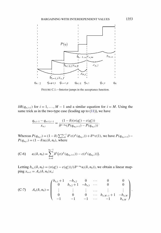
BARGAINING WITH INTERDEPENDENT VALUES 1353
FIGURE C.1.—Interior jumps in the acceptance function.
δR(qn�i+1) for i = 1� � � � �M − 1 and a similar equation for i =M . Using thesame trick as in the two-type case (leading up to (11)), we have
qn�i−1 − qn+1�i−1
xn�i= (1 − δ)(v(q∗
1)− c(q∗1))
δn−n0(P(qn0�i+1)− P(qn0�i))�
Whereas P(qn0�i)= (1 −δ)∑n0−1k=0 δ
kc(tk(qn0�i))+δn0c(1)� we have P(qn0�i+1)−P(qn0�i)= (1 − δ)ai(δ�n0)� where
ai(δ�n0)=n0−1∑k=0
δk(c(tk(qn0�i+1))− c(tk(qn0�i))
)�(C-6)
Letting bn�i(δ�n0)= (v(q∗1)− c(q∗
1))/(δn−n0ai(δ�n0)), we obtain a linear map-
ping xn+1 =An(δ�n0)xn:
An(δ�n0)=
bn�1 + 1 −bn�2 0 · · · 0 0
0 bn�2 + 1 −bn�3 · · · 0 0���
������ · · · ���
���0 0 0 · · · bn�M−1 + 1 −bn�M
−1 −1 −1 · · · −1 bn�M
�(C-7)
1354 R. DENECKERE AND M.-Y. LIANG
Using the fact that c(·) is constant over [q∗1 − ε0� q
∗1 + ε0], we know that
c(tk(qn0�i+1))− c(tk(qn0�i))= 0 for k= 0�1� � � � � n0 −N . Hence we may rewrite(C-6) as
ai(δ�n0)=N−1∑k=1
δn0−(N−k)(c(tn0−N+k(qn0�i+1))− c(tn0−N+k(qn0�i)))�(C-8)
Third, define Ci = {∑N−1k=1 (c(t
n0−N+k(qn0�i+1))− c(tn0−N+k(qn0�i))) :δ ∈ (0�1)}.Note that by definition both n0 and t(·) are functions of δ� Hence, it is con-ceivable that Ci contains infinitely many elements. Nevertheless, because c(·)takes on at most M̄ different values in (q∗
1 + ε0�1], there are only finitely manyelements in Ci.
Fourth, let a′ ∈ C = C1 ×C2 × · · · ×CM and �M(a′)= {δ ∈ (0�1) :a′ ∈C}.In the next paragraph, we will show that there exists a δa′ ∈ (0�1) and an
integer n′0 ∈ (n0�2n0) such that for δ ∈ �M(a′) ∩ (δa′�1), at least one element
in xn′0
is negative. Let δ0 = max{δa′ :a′ ∈ C1 × C2 × · · · × CM}. Because thereare only finitely possible a′, we know δ0 exists and is strictly less than 1. Ap-plying the argument for all possible a′, we conclude that for δ ∈ (δ0�1), thereexists some integer n ∈ (n0�2n0) such that at least one element in xn is neg-ative, which yields a contradiction to the hypothesis #P((q2n0+1� q2n0]) = M .This then completes the proof of Step 2. Henceforth, we therefore consideronly the case where a′ ∈C1 ×C2 × · · · ×CM and δ ∈ �M(a′).
Given two functions of δ, f (δ) ∈ R and g(δ) ∈ R+, we write
f =O(g)if there exists a δ′ < 1 and a constant K > 0 such that for δ > δ′, we have|f (δ)| ≤Kg(δ). By (C-8) we have
ai(δ�n0)= (1 − ε′)(1 +O(1 − δN))a′i�(C-9)
Define bi(ε′)= limδ→1 bn0�i(δ�n0)= (v(q∗1)− c(q∗
1))/((1 − ε′)a′i) and
A(ε′)= limδ→1
An0(δ�n0)�(C-10)
Let λ1�λ2� � � � � λM be the eigenvalues of A(ε′) such that |λ1| ≥ |λ2| ≥ · · · ≥|λM |, where | · | is the absolute value of a complex number, i.e., |α + βi| =√α2 +β2. To simplify the argument, we assume all the eigenvalues are real
and |λ1|> |λ2|> · · ·> |λM |.45 From Claim 4(a) below, we have λ1 > λ2 > · · ·>
45By slightly modifying the proof, we get the same result when some eigenvalues have the sameabsolute value or when they are complex numbers.
BARGAINING WITH INTERDEPENDENT VALUES 1355
λM > 0. Let vi be the eigenvector for A(ε′) that corresponds to λi. For anyvector y = (y1� � � � � yM) ∈ R
M , define
β(y)=M∑i=1
yi�(C-11)
We select vi such that β(vi) = 1 for all i = 1� � � � �M . Now expand any vectorxn ∈ R
M++ on {v1� � � � � vM}, the eigenspace of A(ε′):
xn =M∑i=1
rn�ivi� where rn�i ∈ R�(C-12)
Let
κn = δn−n0(1 +O(1 − δN))�(C-13)
let ei be the ith unit vector in RM , and select αi such that eM = ∑M
i=1 αivi� Thenusing (C-7), (C-9), and (C-10), we have
xn+1 =An(δ�n0)xn = 1κn(A(ε′)− (1 − κn)I)xn +
(1 − κnκn
β(xn)
)eM(C-14)
= 1κn
M∑i=1
((λi − (1 − κn))rn�i + (1 − κn)β(xn)αi
)vi�
From (C-12) and (C-14), we have
rn+1�i = 1κn
((λi − (1 − κn))rn�i + (1 − κn)β(xn)αi
)�(C-15)
For any k and any two vectors x(δ)� y(δ) ∈ Rk, define x ≈ y if limδ→1 xi/
yi = 1 for i = 1� � � � �k. Using (C-15), Claim 2 below establishes that xn+1 ≈
rn+1�1v1 for some n < 2n0(δ�ε′). Therefore, from Claim 4(b), we obtain the
desired result that for sufficiently large δ, there exists an integer n ∈ (n0�2n0)such that at least one element in xn is negative, which yields a contradiction.
PROOF OF STEP 3: We do this in four steps:Step 3.1. Let n2(ε�δ) = 2n̂ − n1 and T = (n2(ε�δ) − n1(ε�δ))ζ. Show that
δ2ρ2(ε)≤ e−rT < ρ2(ε).Because e−rT = δn2−n1 = δ2(n̂−n1) and δρ(ε) ≤ δn̂−n1 < ρ(ε) (defined in
Step 1), we have δ2ρ2(ε)≤ e−rT < ρ2(ε).Step 3.2. Show that qn2 > q
∗1 − 5ε1.
For n≥ n1 define
m̃n+1 = δ−(n−n1−1)ρ(ε)m̃n = · · · = (δ−(n−n1−1)/2ρ(ε)
)n−n1mn1+1�(C-16)
1356 R. DENECKERE AND M.-Y. LIANG
Combining the outer equalities in (C-16) and then substituting n by n2 − i andn1 + 1 by n1 + i, we obtain m̃n2+1−i = (δ−(n2−n1)/2+iρ(ε))n2−n1−2i+1m̃n1+i for i =1� � � � � n̂− n1. Combining with n2 − n1 = 2(n̂− n1) and δ−(n̂−n1)+1ρ(ε) ≤ 1 fori = 1� � � � � n̂− n1, we have δ−(n2−n1)/2+iρ(ε) = δ−(n̂−n1)+iρ(ε) ≤ 1 and n2 − n1 −2i+ 1> 0, which implies m̃n2+1−i ≤ m̃n1+i. Note that n1 + i≤ n̂≤ n̄, so it followsfrom (C-2) that m̃n1+i =mn1+i. Hence,
∑n2i=n1+1 m̃i ≤ 2
∑n̂
i=n1+1 m̃i ≤ 2(qn1 − qn̂).From Step 1, q∗
1 − ε1 < qn̂ < qn1 ≤ q∗1 + ε1, we obtain qn1 − qn̂ < 2ε1 so that∑n2
i=n1+1 m̃i < 4ε1.From the construction of qn in Appendix A and (C-2), we know that if qn −
m̃n+1 ≥ q∗1 − ε0, thenmn+1 = m̃n+1. Suppose now that qk − m̃k+1 ≥ q∗
1 − ε0 holdsfor all n1 ≤ k≤ n− 1. Then qn − m̃n+1 = qn1 − ∑n+1
i=n1+1 m̃i ≥ qn1 − ∑n2i=n1+1 m̃i >
q∗1 − 5ε1 > q
∗1 − ε0. Thus we have mn = m̃n for all n1 ≤ n ≤ n2, so qn2 = qn1 −∑n2
i=n1+1 m̃i > q∗1 − 5ε1.
Step 3.3. Let t ′ = (n̄− n2)ζ� Show that there exists some J > 0 such that forall sufficiently large δ, we have e−rt′ ≥ (1 − ε)J .
Since ρ(ε) < 1, Claim 6 below implies that there exists an integer j > 0 suchthat for all sufficiently large δ, we havemn+1/mn ≥ ρ(ε)j for n=N−1� � � � � n1.Hence, mn1+1 ≥ ρ(ε)j(n1−N+2)mN−1. We now claim that we can obtain the de-sired result by selecting J = j + 1. Let j′ = j(n1 − N + 2). If limδ→1qn2+j′ <q∗
1 − ε0, then we immediately have e−rt′ ≥ δj′ ≥ δn1j = (1 − ε)j > (1 − ε)J for
sufficiently large δ.Suppose limδ→1qn2+j′ ≥ q∗
1 − ε0. From (C-16) and n2 = 2n̂− n1, we have
limδ→1
mn2+j′ = limδ→1
(δ−(n2+j′−n1−2)/2ρ(ε)
)n2+j′−n1−1mn1+1(C-17)
≥ limδ→1
(δ−(n̂−n1)−(j′−2)/2ρ(ε)
)2(n̂−n1)+j′−1ρ(ε)j
′mN−1�
Because ρ(ε) > δn̂−n1 , we can rewrite (C-17) as
limδ→1
mn2+j′ > limδ→1
δ−(j′−2)(n̂−n1)−(j′−2)(j′−1)/2+j′(n̂−n1)mN−1(C-18)
= limδ→1
δ2(n̂−n1)−(j′−2)(j′−1)/2mN−1�
Since δ−1/2 > 1, limδ→1 j′ = ∞, and δ2(n̂−n1) ≥ δ2ρ2(ε), (C-18) implies
limδ→1mn2+j′ ≥ ρ2(ε)mN−1. By the definition of N (right after (C-7)), we haveqN−1 > q
∗1 + ε0. Thus by Lemma C-1, we have mN−1 ≥ η. Note that mn is in-
creasing in n for n > n̂. Hence, we have mn ≥ ηρ2(ε) for n = n2 + j′� � � � � n̄.Combining with qn2+j′ − qn̄ < 2ε0, we obtain n̄− (n2 + j′)≤ 2ε0/(ηρ(ε)). Notethat for all sufficiently large δ we have 2ε0/(ηρ(ε))≤ n1. Hence, for sufficientlylarge δ, we obtain e−rt′ = δn̄−n2 ≥ δj′+2ε0/(ηρ(ε)) ≥ δn1j+n1 ≥ (1 − ε)J .
Step 3.4. Show that P̃(q∗1)= p∗
1.
BARGAINING WITH INTERDEPENDENT VALUES 1357
From optimality of the acceptance decision of seller qn1 , we have P(qn1)−c(qn1) ≥ δn1(c(1)− c(qn1)). Hence, (1 − ε)c(1) ≤ P(qn1) ≤ c(1). Steps 1, 3.1,and 3.3 then yield that
limζ→0
e−r(n̄−N)ζ ≤ limζ→0
e−rT ≤(
v(q∗1)− c(q∗
1)
(1 − ε)c(1)− c(q∗1)
)2
and
limζ→0
e−r(n̄−N)ζ ≥ (1 − ε)J+1 limζ→0
e−rT ≥ (1 − ε)J+1
(v(q∗
1)− c(q∗1)
c(1)− c(q∗1)
)2
for all sufficiently small ε. Whereas limζ→0 e−r(n̄−N)ζ does not depend on ε, we
obtain that limζ→0 e−r(n̄−N)ζ exists and equals (v(q∗
1)− c(q∗1))
2/(c(1)− c(q∗1))
2.Therefore, the limiting delay in [q∗
1 − ε0� q∗1 + ε0] is T1. Note that P(q∗
1 − ε0)=∑n̄−Nk=0 (1 − δ)(δkc(tk(qn̄))) + δn̄−N+1P(tn̄−N+1(qn̄)) and that c(tk(qn̄)) = c(q∗
1)for all k= 0� � � � � n̄−N and tn̄−N+1(qn̄) > q
∗1 + ε0. Hence, by letting δ→ 1, we
have
P̃(q∗1 − ε0)= c(q∗
1)
(1 −
(v(q∗
1)− c(q∗1)
c(1)− c(q∗1)
)2)+
(v(q∗
1)− c(q∗1)
c(1)− c(q∗1)
)2
c(1)
= p∗1�
Note that from Corollary 1 we have P̃(q∗1 + ε0)= c(1). Because ε0 can be arbi-
trary small and P̃ is left-continuous as defined in Section 5, we have P̃(q∗1)= p∗
1.This completes the proof of Step 3.
PROOF OF STEP 4: Similarly to the proof that P̃(q) = c(1) for q ∈ (q∗1�1],
first define
q̃= inf{q : lim
ζ→0P(q)= p∗
1
}�(C-19)
Note that by Step 3 we have P̃(q∗1) = p∗
1. Hence, q̃ is well defined. Similarlyto the argument in Corollary 1, we can show that q̃ = q∗
2, i.e., that the buyer’slimiting surplus is equal to R̃(q) for all q ≥ q∗
2 and that the seller’s limitingacceptance function is equal to p∗
1 on the interval (q∗2� q
∗1]. Q.E.D.
Proofs of Claims 1–6
CLAIM 1: We have #P((qn0� qn0−1])≤ #c((q∗1�1]).
PROOF: We show this by induction: For any qn > q∗1 if #c((qn�1]) = M�
then #P((qn�qn−1]) ≤ M . For n = 1, because P(q) = (1 − δ)c(q) + δc(1),
1358 R. DENECKERE AND M.-Y. LIANG
#P((q1�1]) = #c((q1�1]). Suppose the statement is true for n ≥ 1, i.e.,#c((qn�1]) =M ′ and #P((qn�qn−1]) ≤M ′. Now suppose #c((qn+1�1]) =M�Then #c((qn+1�qn])=M −M ′. Note that P(q)= (1 − δ)c(q)+ δP(t(q)) andt(q) ∈ (qn�qn−1] for q ∈ (qn+1� qn]. Hence, if q is a discontinuity point of P ,then q is a discontinuity point either of c(·) or of P(t(·)), or of both. Be-cause t(·) is increasing, P(t(q)) can have at most M ′ discontinuity points forq ∈ (qn+1�qn]. Furthermore, because c(·) and P(t(·)) are increasing functions,#P((qn+1� qn]) is at most (M −M ′)+M ′ =M . Hence, we can conclude that#P((qn0� qn0−1])≤ #c((qn0�1])= #c((q∗
1�1]). Q.E.D.
CLAIM 2: If for n = n0 + 1� � � � �2n0, xn+1 = An(δ�n0)xn = κ−1n (
∑M
i=1((λi −(1 − κn))rn�i + (1 − κn)β(xn)αi)vi) and κn = δn−n0(1 + O(1 − δN)), then thereexists 1< θ< 2 such that xn′ ≈ rn′�1v1, where n′ = θn0(δ�ε
′).
PROOF: To prove this claim first notice that A(ε′) (defined in (C-10)) de-pends only on c(·) and v(·). Therefore, λi, vi, and αi are constant in δ. How-ever, because β(xn)= ∑M
i=1 xn�i = qn−qn+1 =mn+1 goes to 0 as δ→ 1, we havelimδ→1 xn�i = 0. Thus from xn = ∑M
i=1 rn�ivi, we have limδ→1 rn�i = 0 for all i =1� � � � �M . Hence, to show that xn′ ≈ rn′�1v1, we have to show limδ→1 rn′�i/rn′�1 = 0for i= 2� � � � �M or, equivalently, limδ→1 rn′�1/β(xn′)= 1. Note that if the map-ping from xn to xn+1 were exactly A(ε′) and if rn0�1 �= 0, then because λ1 is thedominant eigenvalue of A(ε′) and n′ → ∞ as δ→ 1, the result would be true.
However, the fact that An(δ�n0) �= A(ε′) introduces the error term (1 −κn)β(xn)αi in (C-14) and (C-15). Accordingly, we divide the proof into threecases, depending on the relative size of the starting coefficient rn0�1 and theerror term, i.e., rn0�1/((1 − κn0)β(xn0)α1). In Case 1, the coefficient rn0�1 domi-nates the error term, so just as above the result will hold. In Case 2, the errorterm dominates rn0�1. We first show that α1 �= 0 so that the error term cannotbe 0. Hence, rn0+1�1 is not zero. Furthermore, after sufficiently many iterations,the errors will accumulate in rn�1, allowing it to dominate (1 − κn)β(xn)α1. Wecan then apply the same argument as in Case 1. Case 3 considers the situationwhere rn�1 and (1 − κn)β(xn)α1 have the same magnitude as δ→ 1, so that itis possible to have |(rn+1�1)/rn�1|< λ2. Hence, it is conceivable that rn�1 remainsrelatively small compared to rn�2, even after many iterations. For this case weargue that there exists no λ1 and λ2 such that rn�1 and (1 − κn)β(xn)α1 canmaintain the same relative magnitude for so many periods. We then reduce toeither Case 1 or Case 2.
Let N ′ = 1/√ζ so that limδ→1N
′ = ∞ and limδ→1 δN′ = 1. Hence limδ→1(1 −
κn0+N ′) = 0 and limδ→1An0+N ′(δ�n0 + N ′) = A(ε′). Define γj = rj�1/((1 −κj)β(xj)α1). Consider the following three cases:
CASE 1—limδ→1 |γn0 | = ∞: Suppose limδ→1|rn0+N ′�1/β(xn0+N ′)| = ψ1 > 0.Applying Claim 3, we obtain that there exists an integer N0 such thatlimδ→1 rn0+N ′+N0�i/rn0+N ′+N0�1 = 0 for i = 2� � � � �M . Therefore, xn0+N ′+N0 ≈
BARGAINING WITH INTERDEPENDENT VALUES 1359
rn0+N ′+N0�1v1. Whereas limδ→1 δN ′+N0 = 1, we haveN ′ +N0 < n0 for δ sufficiently
close to 1.We will show that limδ→1|rn0+N ′�1/β(xn0+N ′)| is indeed strictly greater than
zero. Suppose to the contrary that there exists a sequence {δk} such thatlimδk→1 |rn0+N ′�1/β(xn0+N ′)| = 0. Claim 3 implies limδk→1 |rn0+l�1/β(xn0+l)| = 0for all l = 0� � � � �N ′. Whereas β(xn)= ∑M
k=1 rn�k, we obtain that there exists anonempty set J(l)⊆ {2� � � � �M} such that ¯limδk→1|rn0+l�m/β(xn0+l)|> 0 for anym ∈ J(l) and l = 0�1� � � � �N ′. Let j0 = minJ(0) and select a subsequence {δ′
k}such that ψ2 = limδ′
k→1 |rn0�j0/β(xn0)|> 0. Claim 3 implies that there exists a fi-
nite integer N0 such that limδ′k→1 |rn0+N0�j0/β(xn0+N0)| = 1. Because N0 does not
depend on δ, we have that the mapping∏N0
i=0An0+i(δ�n0) is continuous in ζ,that β(xn0+N0)= (c1 +O(ζ))β(xn0), and that rn0+N0�1 = (c2 +O(ζ))rn0�1, wherec1 and c2 are some nonzero constants. Therefore, limδ′
k→1 γn0+N0 = ∞. For any
ξ > 0, let ρ0N′ = min{l ≥N0 : limδk′ →1 |rn0+l�j0/β(xn0+l)|< 1 − ξ}.
Now suppose first that limξ→0 ρ0 ≥ 1. Using limδk′→1β(xn0+N0+i+1)/β(xn0+N0+i)= λj0 and limδk′ →1 rn0+N0+i+1�1/rn0+N0+i�1 = λ1 for i= 0� � � � � ρ0N
′, wehave that limδk′ →1 γn0+N0+i is increasing in i. This implies that limδk′→1 γn0+N0+i =∞. Hence, for sufficiently large δ, there exists ξ0 ∈ (0� (λ1 − λj0)/4) such that
∣∣∣∣ rn0+N ′�j0rn0+N ′�1
∣∣∣∣= ∣∣((λj0 − (1 − κn0+N ′−1))rn0+N ′−1�j0
+ κn0+N ′−1(1 − κn0+N ′−1)β(xn0+N ′−1)αj)
× ((λ1 − (1 − κn0+N ′−1))rn0+N ′−1�1
+ κn0+N ′−1(1 − κn0+N ′−1)β(xn0+N ′−1)α1
)−1∣∣≤ λj0 + ξ0
λ1 − ξ0·∣∣∣∣ rn0+N ′−1�j0
rn0+N ′−1�1
∣∣∣∣���
≤(λj0 + ξ0
λ1 − ξ0
)N ′−N0
·∣∣∣∣ rn0+N0�j0
rn0+N0�1
∣∣∣∣�Observe that rn0+N0�1r
−1n0+N0�j0
(1−κn0+N0)−1 = γn0+N0r
−1n0+N0�j0
α1β(xn0+N0) and thatthe latter converges to ∞ as δ→ 1. Furthermore, it follows from Courant andJohn (1965, pp. 250 and 253) that
limζ→0
(1 − κn0+N0
)−1(λj0 + ξ0
λ1 − ξ0
)N ′−N0
= limζ→0
e−1/√ζ
ζ= 0�
1360 R. DENECKERE AND M.-Y. LIANG
Hence, we have limδik→1 |rn0+N ′�jr
−1n0+N ′�1| = 0, which contradicts that
limδik→1 |rn0+N ′�j/β(xn0+N ′)| = 1.
Second, suppose that limξ→0 ρ0 < 1. Claim 3 implies that there existj1 = minJ(ρ0N
′) < j0, N1 < ∞, and a subsequence {δ′′k} such that
limδ′′k→1 |rn0+ρ0N
′+N1�j1/β(xn0+ρ0N′+N1)| = 1. Similarly to above, define ρ1N
′ =min{l ≥ N1 : limδ′′
k→1 |rn0+ρ0N
′+l�j1/β(x′n0+ρ0N
′+l)| < 1 − ξ}. Suppose limξ→0(ρ0 +ρ1)≥ 1. Applying a similar argument as above, we have
∣∣∣∣ rn0+N ′�j1rn0+N ′�1
∣∣∣∣ ≤(λj1 + ξ1
λ1 − ξ1
)(1−ρ0)N′−N1
∣∣∣∣ rn0+ρ0N′+N1�j1
rn0+ρ0N′+N1�1
∣∣∣∣�and thus limδ′′
k→1 |rn0+N ′�j1/β(xn0+N ′)| = 0, a contradiction. If limξ→0(ρ0 +
ρ1) < 1, then as above we can define j2 < j1 and ρ2, and repeat the sameprocess. Whereas j0 ≤M , it takes at most M − 1 iterations to complete theproof.
CASE 2—limδ→1 |γn0 | = 0: From Claim 5, we know α1 �= 0. Hence, rn0+1�1 ≈
α1(1 − κn0)β(xn0). This implies that for all n > n0 + 1� rn�1 and α1 have thesame sign. Therefore, from (C-15) we have rn+1�1r
−1n�1 > λ1 − (1 −κn) for all n >
n0 + 1. Let n′′(δ�ε′� ε′′) such that δn′′−n0 = 1 − ε′′ > 1 − ε′. Hence 1 − κn′′ ≈ ε′′
and β(xn′′) = O(|rn′′�1|). It follows that limδ→1|rn′′�1/β(xn′′)| = ψ2 > 0. Using asimilar argument as in Case 1, where n′′ takes the role of n0, we obtain xn′ ≈
rn′�1v1 when δ is sufficiently large, where n′ = n′′ +N0 < 2n0.
CASE 3— ¯limδ→1|γn0 | > 0 and limδ→1|γn0 | < ∞: From (C-15) we obtainrn0+1�1r
−1n0�1
= κ−1n0(λ1 − (1 − κn0)+ γ−1
n0). Hence, if γn0 < 0� it is possible to have
rn0+1�1r−1n0�1< rn0+1�2r
−1n0�2� a potential threat to our goal xn ≈ rn�1v1. Hence for this
case, we need a better estimate of rn�1. To simplify the argument, we consideronly the worst case: γn0 < 0 and β(xn0) = O(|rn0�2|). From Case 1, we obtainxn ≈ λ
n−n01 rn0�1v1 + λ
n+1−n02 rn0�2v2 for n0 +N ′ ≤ n ≤ n0 + 2N ′. If there exists an
n ≤ n0 + 2N ′ such that either limδ→1 |γn| = 0 or limδ→1 |γn| = ∞ holds, thenby applying Case 1 or Case 2, respectively, we obtain xn′ ≈ rn′�1v1 for somen′ < 2n0, which completes the proof.
Now consider the case that for every n = n0 + N ′� � � � � n0 + 2N ′� thereexists a sequence {δi}∞
i=0 such that limδi→1 |γn| ∈ (0�∞). This implies xn ≈
λn−n02 rn0�2v2�β(xn)= λn−n0
2 rn0�2 +O(1−κn) andβ(xn+1)/β(xn)= λ2 +O(1−κn)�Whereas limδ→1 κn = 1� using (C-15) recursively, we have
rn�1 ≈ α1(1 − κn0)β(xn0)
(γn0λ
n−n01 +
n−n0−1∑i=0
λn−1−n0−i1
β(xn0+i)β(xn0)
)�(C-20)
BARGAINING WITH INTERDEPENDENT VALUES 1361
Letting fn0(N′) = γn0 + ∑N ′
i=0 λ−i−11 β(xn0+i)/β(xn0) and using β(xn+1)/
β(xn)= λ2 +O(1 − κn), we can further rewrite (C-20) to
rn�1 ≈ α1(1 − κn0)β(xn0)
(λn−n01 fn0(N
′)+n−n0−1∑k=N ′+1
λn−1−n0−k1 λk2
)�(C-21)
Using (C-21), β(xn0)≈ rn0�2, and β(xn)≈ λn−n02 rn0�2� we obtain
γn = rn�1
α1(1 − κn)β(xn) ≈
(λ1
λ2
)n−n0
fn0(N′)+ 1
λ2
n−n0−1∑k=N ′+1
(λ1
λ2
)n−n0−k
= −λ1
λ2(λ1 − λ2)+
(λ1
λ2
)n−n0−N ′((λ1
λ2
)N ′
fn0(N′)+ 1
λ1 − λ2
)�
Note that given λ1λ−12 > 1, to obtain limδi→1 |γn| ∈ (0�∞) for all n = n0 +
N ′� � � � � n0 + 2N ′ requires (λ1λ−12 )
N ′fn0(N
′) + 1/(λ1 − λ2) ≡ 0. Hence, γn ≈
−λ1λ−12 /(λ1 − λ2) for all n = n0 +N ′� � � � � n0 + 2N ′. On the other hand, from
(C-15) andβ(xn+1)/β(xn)≈ λ2, we have γn+1 = rn+1�1(α1(1−κn+1)β(xn+1))−1
≈
λ1λ−12 γn + 1. Combining with γn+1 ≈ γn, we obtain γn ≈ λ1λ
−12 γn + 1. Hence,
−λ1λ−12 (λ1 − λ2)
−1≈ γn ≈ −(λ1 − λ2), which implies λ1 = λ2, a contradic-
tion. Q.E.D.
CLAIM 3: Let n be any function of δ that satisfies limδ→1 δn = 1 − ε′. If
there exists an i < M such that limδ→1|rn�i/β(xn)| = ψi > 0, then for all j =i + 1� � � � �M there exists an integer N0, which is independent on δ, such thatlimδ→1 |rn+N0�jr
−1n+N0�i
| = 0.
PROOF: Let Σ1 = {y ∈ RM :β(y) = 1} and Σ0 = {y ∈ R
M :β(y) = 0}� There-fore, v1� � � � � vM and xn/β(xn) belong to Σ1. Denote uk = vk−v1 ∈ Σ0 for k≥ 2.Note that {uk}nk=2 is a basis for Σ0. By (C-12) we have β(xn) = ∑M
k=1 rn�k, sorn�1/β(xn)= 1 − ∑M
k=2 rn�k/β(xn). Hence
xn
β(xn)=
M∑k=1
rn�k
β(xn)vk = v1 +
n∑k=2
rn�k
β(xn)uk ∈ Σ1 ∩ R
M++�
This implies that∑n
k=2 rn�kuk/β(xn) ∈ Σ0 ∩ (Rn++ − v1), which is a bounded
subset of Σ0. Because {uk}nk=2 is a basis for Σ0, rn�k/β(xn) is bounded fork = 2� � � � �M . Hence so is rn�1/β(xn). Note that this bound does not dependon xn.46 Therefore, there exists a constant ψ such that |rn�k/β(xn)|<ψ for all
46We are grateful to Tai-Peng Tsai for suggesting the line of argument above.
1362 R. DENECKERE AND M.-Y. LIANG
δ < 1 and k= 1� � � � �M . Let i be as in the statement of the claim and, for anyξ > 0, choose N0 such that (λi+1λ
−1i )
N0 < ξ. Whereas An(δ�n) converges toA(ε′) as δ→ 1 and xn+N0 = ∏N0−1
k=0 An+k(δ�n)xn, we have, for any ξ′ < ξλN0i �
that there exists δ′ < 1 such that, for all δ > δ′, we have (A(ε′)N0 − ξ′)xn ≤xn+N0 ≤ (A(ε′)N0 + ξ′)xn. Hence, for any j = i+ 1� � � � �M , we obtain
limδ→1
∣∣∣∣ rn+N0�j
rn+N0�i
∣∣∣∣< limδ→1
(λN0j + ξ′)|rn�j|
(λN0i − ξ′)|rn�i|
<λN0i+1 + ξλN0
i
λN0i − ξλN0
i
· ψψi
≤ 2ξ1 − ξ · ψ
ψi�
Because ξ is arbitrary, we have limδ→1 |rn+N0�jr−1n+N0i
| = 0. Q.E.D.
CLAIM 4: (a) For i = 1� � � � �M�λi > 0 and (b) if xn ≈ rn�1v1, then for suffi-ciently large δ at least one element in xn is negative.
PROOF: (a) Let h(λ)= det(A(ε′)− λI)� It can be shown that h(y) > 0 forall y ≤ 0.
(b) It can also be shown that h(bj + 1) < 0 for all j = 1� � � � �M − 1 andh(bM) < 0. Hence there exists at least one eigenvalue in (0� b̄), where b̄ =min{b1 + 1� � � � � bM−1 + 1� bM} > 0. From
∑M
j=1 λj = ∑M−1j=1 (bj + 1) + bM , we
know that λ1 > b̄ > 0� If b̄= bj + 1 for some j <M , then (A(ε′)− λ1I)v1 = 0implies (bj + 1 − λ1)v1�j − bj+1v1�j+1 = 0. Hence, either sign(v1�j) �= sign(v1�j+1)or v1�j = v1�j+1 = 0. However, v1�j = v1�j+1 = 0 induces v1 = 0, which yields acontradiction. We can therefore conclude that sign(v1�j) �= sign(v1�j+1). A simi-lar argument applies to the case where b̄= bM . Q.E.D.
CLAIM 5: For some α ∈ RM and α1 �= 0� eM = ∑M
i=1 αivi� i.e., eM cannot begenerated by {v2� � � � � vM}.
PROOF: Let S be the space generated by v2� � � � � vM and let V = [v1v2 · · ·vM].Suppose eM ∈ S, i.e., eM = ∑M
i=2 αivi = V α for some α �= 0 with α1 = 0� Thenusing V −1AV α = �α, we have V −1AeM = (0�λ2α2�λ3α3� � � � � λMαM)
′. Pre-multiplying by V yields (0� � � � �0�−bM�bM)′ = V (0�λ2α2�λ3α3� � � � � λMαM)
′ =∑M
i=2 λiαivi ∈ S� Whereas both −bMeM−1 + bMeM and eM are in S, and whereasS is a vector space, we know that eM−1 ∈ S� By induction, we can similarly showthat eM�eM−1� � � � � e1 ∈ S, yielding a contradiction to the idea that S is of di-mension M − 1. Q.E.D.
CLAIM 6: There exists a constant ρ0 > 0 such that for sufficiently large δ, wehave mn+1/mn ≥ ρ0 for n=N − 1� � � � � n1.
PROOF: For anyM ,M ′ ∈ {1� � � � � M̄} andM ≤M ′, let�(M�M ′)= {δ :n(δ) ∈{N − 1� � � � � n1}�#P((qn(δ)+1�qn(δ)]) = M , and #P(qn(δ)� qn(δ)−1) = M ′}. We
BARGAINING WITH INTERDEPENDENT VALUES 1363
claim that there exists no sequence {δk} ∈ �(M�M ′) for which limδk→1mn+1/mn = 0. Consequently, there exists ρ(M�M ′) > 0 such that limδk→1mn+1/mn >ρ(M�M ′) for every sequence {δk} ∈ �(M�M ′). Letting ρ0 = maxM�M ′ ρ(M�M ′)then yields the desired result.
Using the definition of R(·) and the fact that R(qn) − R(qn−1�i) =∫ qn−1�iqn
(v(z)− P(t(z)))dz, the following equation holds for any i= 1� � � � �M ′:
R(qn+1)=∫ qn
qn+1
(v(z)− P(qn))
+ δ(∫ qn−1�i
qn
(v(z)− P(t(z)))dz+R(qn−1�i)
)�
Because qn−1�i is feasible from qn+1, we also have
R(qn+1)≥∫ qn−1�i
qn+1
(v(z)− P(qn−1�i)) dz+ δR(qn−1�i)�
Combining the previous two inequalities, and using the fact that P(qn−1�i) =(1 − δ)c(qn−1�i)+ δP(t(qn−1�i)), we then obtain
(P(qn−1�i)− P(qn))mn+1(C-22)
≥∫ qn−1�i
qn
((1 − δ)(v(z)− c(qn−1�i))
− δ[P(t(qn−1�i))− P(t(z))])dz�By definition, the acceptance function is constant over (qn−1�i−1�qn−1�i], soc(z)= c(qn−1�i) for all z ∈ (qn−1�i−1�qn−1�i]. Because v(z)− c(z) > ∆, it followsthat
∫ qn−1�iqn−1�i−1(v(z)− c(qn−1�i)) dz ≥ �xn−1�i > 0.
The definition of qn−1�i implies that t(z) = t(qn−1�i) for z ∈ (qn−1�i−1�qn−1�i].Therefore, for i = 1, (C-22) implies mn+1 ≥ (1 − δk)�xn−1�1/(P(qn−1�1) −P(qn))≥ 0. Using the same arguments as in (C-6) which leads to (C-9), we havelimδk→1(1 − δk)(P(qn−1�1) − P(qn)) > 0� Hence, the hypothesis limδk→1mn+1/mn = 0 implies limδk→1 xn−1�1/mn = 0. By induction, if limδk→1 xn−1�j/mn = 0for j = 1� � � � � i− 1, then (C-22) implies limδk→1 xn−1�i/mn = 0. Hence, we havelimδk→1 xn−1�i/mn = 0 for i = 1� � � � �M ′, contradicting that
∑M ′i=1 xn−1�i/mn = 1.
Q.E.D.
REFERENCES
ADMATI, A., AND M. PERRY (1987): “Strategic Delay in Bargaining,” Review of Economic Studies,54, 345–364. [1311]
AKERLOF, G. A. (1970): “The Market for ‘Lemons’: Quality Uncertainty and the Market Mech-anism,” Quarterly Journal of Economics, 84, 488–500. [1310,1314,1326]
1364 R. DENECKERE AND M.-Y. LIANG
AUSUBEL, L. M., AND R. J. DENECKERE (1989a): “Reputation in Bargaining and Durable GoodsMonopoly,” Econometrica, 57, 511–531. [1325,1326,1347]
(1989b): “A Direct Mechanism Characterization of Sequential Bargaining with One-Sided Incomplete Information,” Journal of Economic Theory, 48, 18–46. [1310,1337]
(1993): “A Generalized Theorem of the Maximum,” Economic Theory, 3, 99–107. [1316]BIKHCHANDANI, S. (1992): “A Bargaining Model with Incomplete Information,” Review of Eco-
nomic Studies, 59, 187–204. [1311]BILLINGSLEY, P. (1968): Convergence of Probability Measures. New York: Wiley. [1346]CHO, I. (1990a): “Characterization of Equilibria in Bargaining Models with Incomplete Informa-
tion,” Unpublished Manuscript, University of Chicago. [1311](1990b): “Uncertainty and Delay in Bargaining,” Review of Economic Studies, 57,
575–595. [1311]COASE, R. H. (1972): “Durability and Monopoly,” Journal of Law and Economics, 15, 143–149.
[1312,1334]COURANT, R., AND F. JOHN (1965): Introduction to Calculus and Analysis. New York: Wiley. [1359]CRAMTON, P., AND J. TRACY (1992): “Strikes and Holdouts in Wage Bargaining: Theory and
Data,” American Economic Review, 82, 100–121. [1309]DENECKERE, R. J. (1992): “A Simple Proof of the Coase Conjecture,” Unpublished Manuscript,
Northwestern University. [1318,1326]EVANS, R. (1989): “Sequential Bargaining with Correlated Values,” Review of Economic Studies,
56, 499–510. [1313]FUDENBERG, D., D. K. LEVINE, AND J. TIROLE (1985): “Infinite-Horizon Models of Bargain-
ing with One-Sided Incomplete Information,” in Game Theoretic Models of Bargaining, ed. byA. Roth. Cambridge, U.K.: Cambridge University Press. [1310,1342]
GUL, F., H. SONNENSCHEIN, AND R. WILSON (1986): “Foundations of Dynamic Monopoly andthe Coase Conjecture,” Journal of Economic Theory, 39, 155–190. [1310,1315,1325]
HICKS, J. R. (1932): The Theory of Wages. London, U.K.: MacMillan. [1309]MYERSON, R. B. (1985): “Analysis of Two Bargaining Problems with Incomplete Information,” in
Game Theoretic Models of Bargaining, ed. by A. Roth. Cambridge, U.K.: Cambridge UniversityPress. [1310,1332]
MYERSON, R. B., AND M. SATTERTHWAITE (1983): “Efficient Mechanisms for Bilateral Trading,”Journal of Economic Theory, 29, 265–281. [1309]
SAMUELSON, W. (1984): “Bargaining under Asymmetric Information,” Econometrica, 52,995–1005. [1310,1332,1334,1342]
VINCENT, D. R. (1989): “Bargaining with Common Values,” Journal of Economic Theory, 48,47–62. [1313,1325]