Barriers to Entry for Young and Beginning

Cattle Producers in Oklahoma

Seth Menefee

Graduate Research Assistant

Department of Agricultural Economics

Oklahoma State University

421D Agricultural Hall

Stillwater, OK 74078

Tel: (405) 612-7708

Email: seth.menefee@okstate.edu

Damona Doye

Regents Professor and Sarkeys Distinguished Professor

Department of Agricultural Economics

Oklahoma State University

529 Agricultural Hall

Stillwater, OK 74078

Email: damona.doye@okstate.edu

Selected Paper prepared for presentation at the Southern Agricultural Economics Association

(SAEA) Annual Meeting, Orlando, Florida, 3-5 February 2013

Copyright 2013 by Seth Menefee and Damona Doye. All rights reserved. Readers may make

verbatim copies of this document for non‐commercial purposes by any means, provided that this

copyright notice appears on all such copies.

1

Objectives

The overall objective of this research is to determine the barriers to entry by young, aspiring

beginning cattle producers in Oklahoma. The specific objectives of this research on beginning

cattle operators are:

1. To identify the start-up capital requirements and potential debt obligations using

different means of financing.

2. To evaluate the effect of differing herd size and off-farm income scenarios in meeting

cash flow obligations.

Background

There has been significant debate regarding the aging farming population in America and

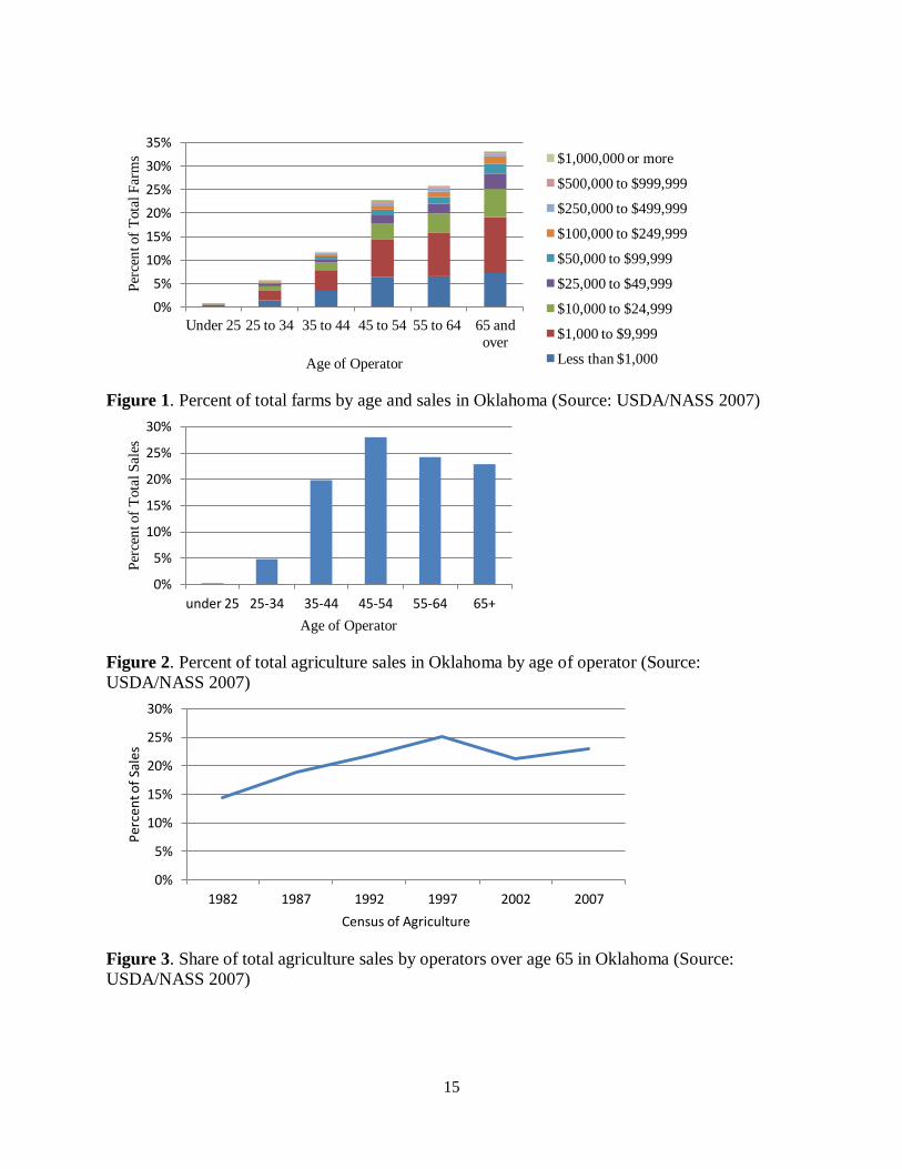
the implications of this trend. USDA data from 2011 indicates that 37% of all cattle farms in the

U.S. are operated by producers over the age of 65. An additional 29% are operated by producers

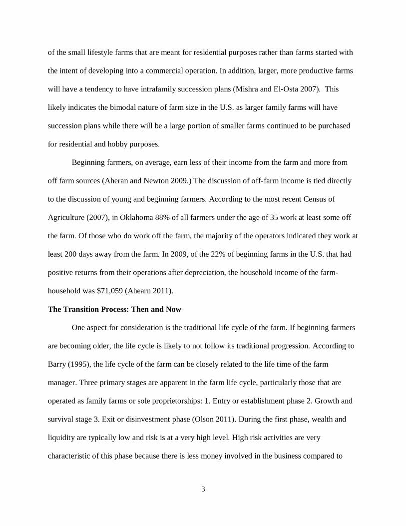
over the age of 55. Oklahoma statistics for farm numbers by age of operator and sales class are

shown in Figure 1. Roughly 6% of all farm operators in Oklahoma are under the age of 35 while

33% of operators are over the age of 65 (USDA/NASS 2007). Further analysis shows that a

large portion of these farms have very limited sales and likely reflect small, hobby farms for

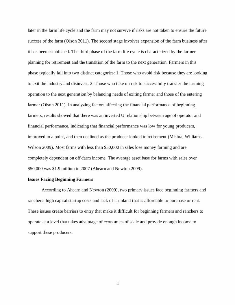
residential purposes. Although the 65 and over age category account for the highest percentage

of total farms, they do not account for majority of the sales as seen in Figure 2. This shows the

tendency for older producers to begin to disinvest in the operation and to not engage in as

intensive activities as the operator reaches a certain age (Mishra, Williams, Wilson 2009).

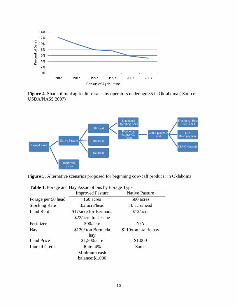
The average age of the primary farm operator has risen from 50.3 in 1978 to 57.1 in

2007. This rising age of the farmer has been a trend for a considerable time, so why the sudden

concern? Dr. Derrell Peel recently referred to the issue as the “demographic cliff” (Oklahoma

2

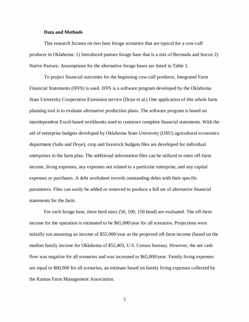
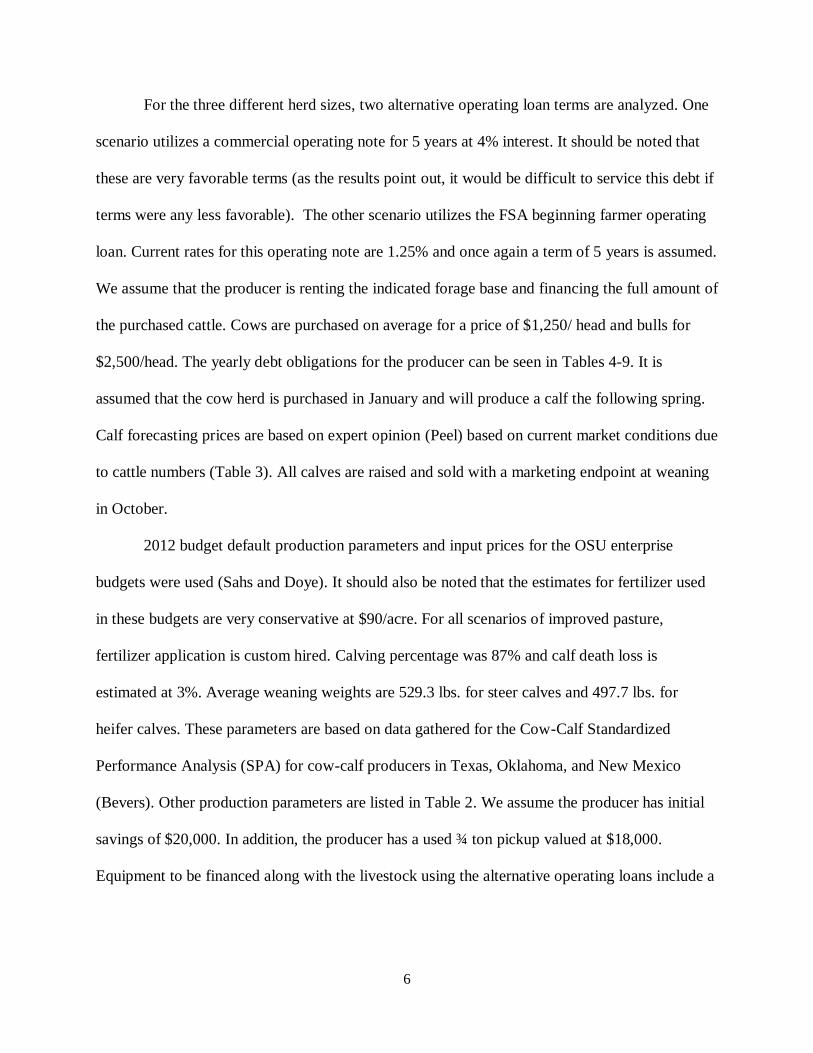
Farm Report). The percent of sales accounted for by operators over the age of 65 has steadily

increased over the last 25 years while the sales accounted for by operators under the age of 35

has declined as seen in Figures 3 and 4. What challenges and barriers to entry do young

producers face as they try to enter the industry? This research focuses particularly on a beginning

cow-calf producer in Oklahoma trying to enter the industry with varying forage bases, herd sizes,

financing terms, and off-farm income.

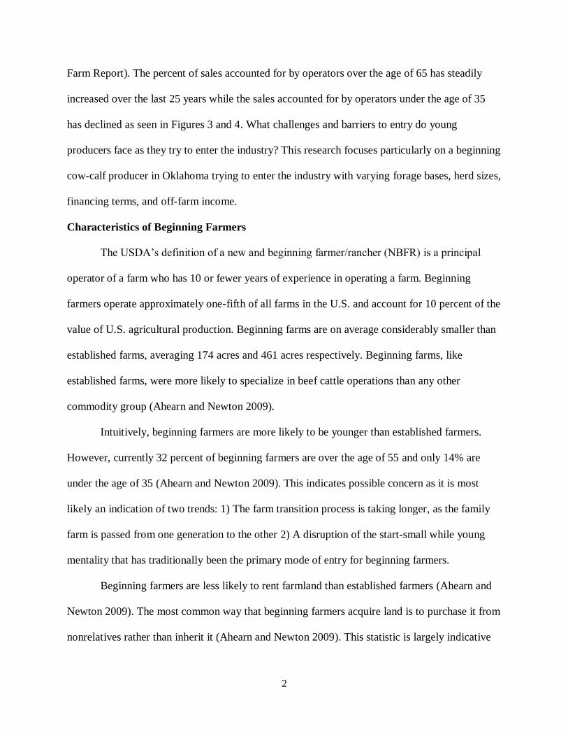
Characteristics of Beginning Farmers

The USDA’s definition of a new and beginning farmer/rancher (NBFR) is a principal

operator of a farm who has 10 or fewer years of experience in operating a farm. Beginning

farmers operate approximately one-fifth of all farms in the U.S. and account for 10 percent of the

value of U.S. agricultural production. Beginning farms are on average considerably smaller than

established farms, averaging 174 acres and 461 acres respectively. Beginning farms, like

established farms, were more likely to specialize in beef cattle operations than any other

commodity group (Ahearn and Newton 2009).

Intuitively, beginning farmers are more likely to be younger than established farmers.

However, currently 32 percent of beginning farmers are over the age of 55 and only 14% are

under the age of 35 (Ahearn and Newton 2009). This indicates possible concern as it is most

likely an indication of two trends: 1) The farm transition process is taking longer, as the family

farm is passed from one generation to the other 2) A disruption of the start-small while young

mentality that has traditionally been the primary mode of entry for beginning farmers.

Beginning farmers are less likely to rent farmland than established farmers (Ahearn and

Newton 2009). The most common way that beginning farmers acquire land is to purchase it from

nonrelatives rather than inherit it (Ahearn and Newton 2009). This statistic is largely indicative

3

of the small lifestyle farms that are meant for residential purposes rather than farms started with

the intent of developing into a commercial operation. In addition, larger, more productive farms

will have a tendency to have intrafamily succession plans (Mishra and El-Osta 2007). This

likely indicates the bimodal nature of farm size in the U.S. as larger family farms will have

succession plans while there will be a large portion of smaller farms continued to be purchased

for residential and hobby purposes.

Beginning farmers, on average, earn less of their income from the farm and more from

off farm sources (Aheran and Newton 2009.) The discussion of off-farm income is tied directly

to the discussion of young and beginning farmers. According to the most recent Census of

Agriculture (2007), in Oklahoma 88% of all farmers under the age of 35 work at least some off

the farm. Of those who do work off the farm, the majority of the operators indicated they work at

least 200 days away from the farm. In 2009, of the 22% of beginning farms in the U.S. that had

positive returns from their operations after depreciation, the household income of the farm-

household was $71,059 (Ahearn 2011).

The Transition Process: Then and Now

One aspect for consideration is the traditional life cycle of the farm. If beginning farmers

are becoming older, the life cycle is likely to not follow its traditional progression. According to

Barry (1995), the life cycle of the farm can be closely related to the life time of the farm

manager. Three primary stages are apparent in the farm life cycle, particularly those that are

operated as family farms or sole proprietorships: 1. Entry or establishment phase 2. Growth and

survival stage 3. Exit or disinvestment phase (Olson 2011). During the first phase, wealth and

liquidity are typically low and risk is at a very high level. High risk activities are very

characteristic of this phase because there is less money involved in the business compared to

4

later in the farm life cycle and the farm may not survive if risks are not taken to ensure the future

success of the farm (Olson 2011). The second stage involves expansion of the farm business after

it has been established. The third phase of the farm life cycle is characterized by the farmer

planning for retirement and the transition of the farm to the next generation. Farmers in this

phase typically fall into two distinct categories: 1. Those who avoid risk because they are looking

to exit the industry and disinvest. 2. Those who take on risk to successfully transfer the farming

operation to the next generation by balancing needs of exiting farmer and those of the entering

farmer (Olson 2011). In analyzing factors affecting the financial performance of beginning

farmers, results showed that there was an inverted U relationship between age of operator and

financial performance, indicating that financial performance was low for young producers,

improved to a point, and then declined as the producer looked to retirement (Mishra, Williams,

Wilson 2009). Most farms with less than $50,000 in sales lose money farming and are

completely dependent on off-farm income. The average asset base for farms with sales over

$50,000 was $1.9 million in 2007 (Ahearn and Newton 2009).

Issues Facing Beginning Farmers

According to Ahearn and Newton (2009), two primary issues face beginning farmers and

ranchers: high capital startup costs and lack of farmland that is affordable to purchase or rent.

These issues create barriers to entry that make it difficult for beginning farmers and ranchers to

operate at a level that takes advantage of economies of scale and provide enough income to

support these producers.

5

Data and Methods

This research focuses on two base forage scenarios that are typical for a cow-calf

producer in Oklahoma: 1) Introduced pasture forage base that is a mix of Bermuda and fescue 2)

Native Pasture. Assumptions for the alternative forage bases are listed in Table 1.

To project financial outcomes for the beginning cow-calf producer, Integrated Farm

Financial Statements (IFFS) is used. IFFS is a software program developed by the Oklahoma

State University Cooperative Extension service (Doye et al.) One application of this whole farm

planning tool is to evaluate alternative production plans. The software program is based on

interdependent Excel-based workbooks used to construct complete financial statements. With the

aid of enterprise budgets developed by Oklahoma State University (OSU) agricultural economics

department (Sahs and Doye), crop and livestock budgets files are developed for individual

enterprises in the farm plan. The additional information files can be utilized to enter off-farm

income, living expenses, any expenses not related to a particular enterprise, and any capital

expenses or purchases. A debt worksheet records outstanding debts with their specific

parameters. Files can easily be added or removed to produce a full set of alternative financial

statements for the farm.

For each forage base, three herd sizes (50, 100, 150 head) are evaluated. The off-farm

income for the operation is estimated to be $65,000/year for all scenarios. Projections were

initially run assuming an income of $55,000/year as the projected off-farm income (based on the

median family income for Oklahoma of $52,403, U.S. Census bureau). However, the net cash

flow was negative for all scenarios and was increased to $65,000/year. Family living expenses

are equal to $60,000 for all scenarios, an estimate based on family living expenses collected by

the Kansas Farm Management Association.

6

For the three different herd sizes, two alternative operating loan terms are analyzed. One

scenario utilizes a commercial operating note for 5 years at 4% interest. It should be noted that

these are very favorable terms (as the results point out, it would be difficult to service this debt if

terms were any less favorable). The other scenario utilizes the FSA beginning farmer operating

loan. Current rates for this operating note are 1.25% and once again a term of 5 years is assumed.

We assume that the producer is renting the indicated forage base and financing the full amount of

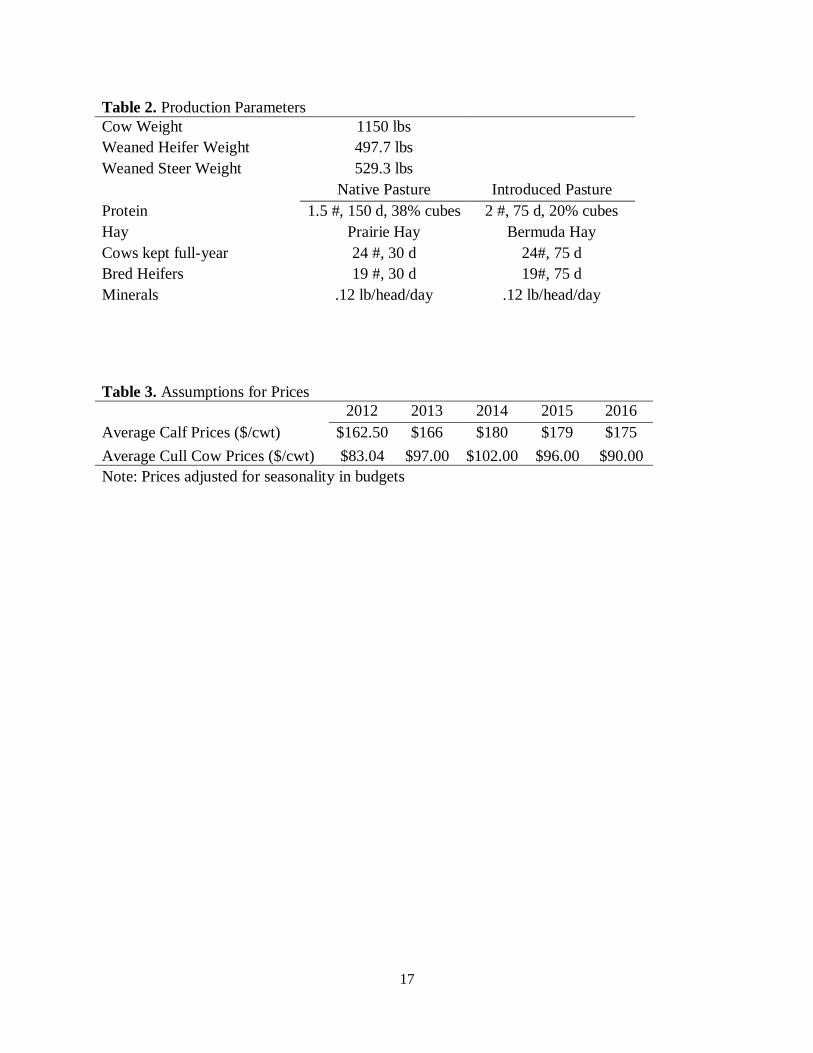
the purchased cattle. Cows are purchased on average for a price of $1,250/ head and bulls for

$2,500/head. The yearly debt obligations for the producer can be seen in Tables 4-9. It is

assumed that the cow herd is purchased in January and will produce a calf the following spring.

Calf forecasting prices are based on expert opinion (Peel) based on current market conditions due

to cattle numbers (Table 3). All calves are raised and sold with a marketing endpoint at weaning

in October.

2012 budget default production parameters and input prices for the OSU enterprise

budgets were used (Sahs and Doye). It should also be noted that the estimates for fertilizer used

in these budgets are very conservative at $90/acre. For all scenarios of improved pasture,

fertilizer application is custom hired. Calving percentage was 87% and calf death loss is

estimated at 3%. Average weaning weights are 529.3 lbs. for steer calves and 497.7 lbs. for

heifer calves. These parameters are based on data gathered for the Cow-Calf Standardized

Performance Analysis (SPA) for cow-calf producers in Texas, Oklahoma, and New Mexico

(Bevers). Other production parameters are listed in Table 2. We assume the producer has initial

savings of $20,000. In addition, the producer has a used ¾ ton pickup valued at $18,000.

Equipment to be financed along with the livestock using the alternative operating loans include a

7

used gooseneck trailer valued at $5,000 and equipment including a chute, portable corrals, and

feeders totaling $11,300.

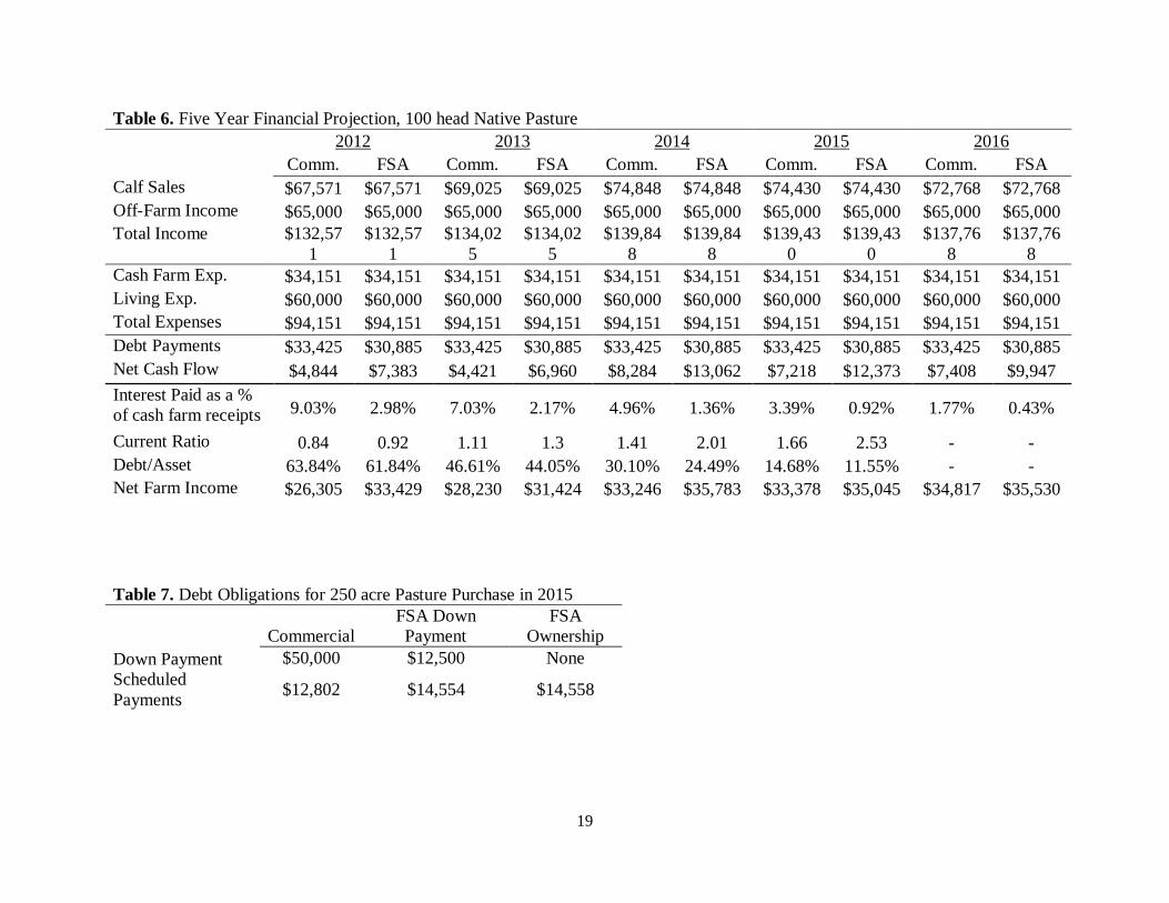
After all base scenarios are constructed and analyzed, a five year projection is made for

the 100 head base scenario to evaluate the operation over the course of the livestock loan (Table

6). One of the biggest challenges of these projections was formulating a strategy for replacing

cull cows and maintaining herd size. Retaining heifers for replacements can be difficult for a

herd this size (Troxel 2007). We assume a culling rate of 10% per year to be sold in October to

be replaced with bred females purchased in December for the following year. This is likely not a

long-term herd management strategy but for cash flow purposes and establishing a cow herd will

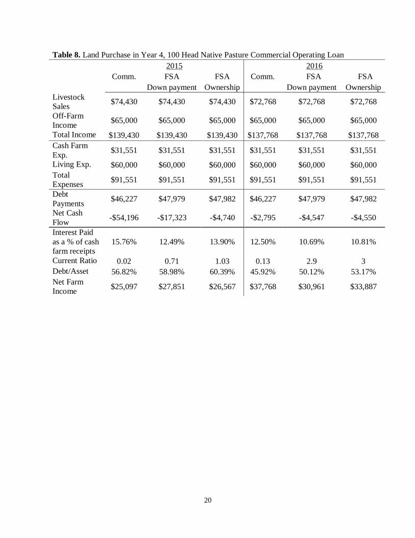
work for this research. In year 4, a land purchase using three alternative methods for financing

the purchase will be evaluated using the 100 head base case scenario (Table 8): 1) A traditional

note with a required 20% down payment, 25 year term, and 4% interest rate 2) The FSA down

payment program that requires 5% down, 20 year term, and 1.5% interest rate for 45% of the

purchase price with the remaining 50% of the purchase price financed using the same terms as

the traditional loan 3) The FSA direct farm ownership loan with no down payment, 3.125%

interest, and a term up to 40 years (25 years is used in scenario) with a maximum amount to be

financed of $300,000. The FSA farm ownership loans require that the operator meet some

specific requirements: 1) Be a beginning farmer (if more than one operator then every operator

must be by definition a beginning farmer) 2) meet the requirements for the specific program the

producer is applying for 3) substantially participate in the operation 4) does not own a farm

greater than 30% of the median farm size in the county 5) For ownership purchases, the applicant

must have participated in the business operation for at least three years (fsa.usda.gov).

Results

8

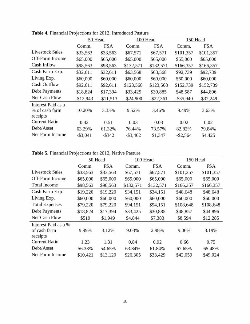
Table 4 indicates that a beginning cow-calf producer will have a very difficult time

having a positive cash flow or net farm income on improved pasture. Even though significantly

less land is required and the land is stocked much more heavily, the additional fertilizer expense

incurred by maintaining the fescue and Bermuda offset this. As Table 4 indicates, cash flow was

negative for all herd sizes but as the herd was expanded to 100 head the producer’s cash supply

was completely depleted and an outstanding balance transferred to the following year. Even

though the beginning producer could sustain small losses from year to year, the introduced

forage base appears to be infeasible for a beginning producer and the five year projection was not

pursued.

The scenarios with the native pasture forage base showed that it was feasible for the

beginning producer to operate (Table 5). Although the native pasture requires more acres and is

less intensively stocked, the native pasture had positive returns for the beginning producer given

the assumptions used. The decreased farm expenses allowed for the producer to have positive

cash flow that will be available for reinvestment.

The terms of the FSA loan helped out considerably for both forage bases. However, the

commercial terms used in this research also result in a feasible plan from a cash flow perspective

for the native pasture. For instance, if the interest rate is 7%, which is more historically normal,

the scheduled debt payment for equipment and 50 head of cattle is $20,438/year for a five year

note compared to the $18,824/year (Table 4) used for the base case here. If the interest rate, were

to increase to 7%, net cash flow would become negative for the 50 head, native pasture scenario.

In these circumstances, the FSA beginning farmer operator loan would be beneficial in helping

reduce payments. Another factor to consider is the initial purchase price for the cattle. Scenarios

were developed based on an initial purchase price of $1,250/head; however, this is likely low

9

given the current market conditions. For instance, if the cattle are purchased for $1,500/head, the

beginning operator would need a 7 year term on their operating note to have positive net cash

flow holding all other assumptions constant.

One assumption of this research that is associated with the herd size is that the cow-calf

operation is heavily supported with off-farm income of $65,000/year. Admittedly, this is likely

high for some parts of rural Oklahoma. Once again, this reinforces previous literature (Ahearn;

Mishra, Williams, and Wilson) that beginning farms are very reliant on off-farm income. Take

for instance, the native pasture 100 head operation utilizing the FSA operating loan. Decreasing

the off-farm income to $55,000/year net cash flow decreased to -$409 from $9,716. The line of

credit analysis points to similar conclusions about the importance of off-farm income.

There are a few other points to consider for the cash flow of the beginning producer. The

first is that at 50 head for the introduced pasture, the operation incurred a cash flow deficit while

the native pasture did not. The reason for this is the additional fertilizer expense costs for the

improved pasture. No matter the scale or off-farm income, fertilizer is a major cash expense at

application during the summer months for summer months and debt payments will be difficult to

make in addition to the operating expenses. In all scenarios, even ones where off-farm income

was increased, the operation was very reliant on the line of credit to meet cash requirements for

fertilizer expenses. The second thing to note is the reliance on the line of credit for the native

pasture even at the 100 head herd size despite having a positive net cash flow. In this research, it

is assumed that the cattle, all other assets, and new borrowing were acquired in January. There is

also another large cash expense early in the year for hay feeding through the winter months. The

operation started off the year at a deficit due to the increased costs for hay and it wasn’t until the

10

calves were sold in October that the operation had a positive net cash flow. This is only minor, as

the line of credit was paid off along with interest at the end of the year.

Where the favorable terms for the FSA operating loan became very helpful was when

saving enough cash to make a down payment for the land purchase. Although the operation had a

negative cash flow in the purchased year, the initial loan for the livestock will be paid off at the

end of the second year of the land note and cash flow will be sufficient to purchase additional

livestock. Purchasing native pasture land for cow-calf producers will be difficult given the large

amount of land required to stock native pasture. Table 7 shows the down payment required along

with the yearly debt obligations for the loan. The land to be purchased is 250 acres of native

pasture to stock 25 moderate sized females. For the FSA farm ownership loans, the farm to be

purchased cannot be over 30% of the median farm size in the county. For example, 250 acres

would be under the limit for Dewey and Kiowa counties but over the limit for Caddo and Kiowa

counties. The FSA ownership loans are helpful in providing an affordable down payment for the

beginning producer but do limit the amount of land that can be purchased in many counties. The

scheduled debt payments for the FSA farm ownership loans prove to be very close given the

assumptions about the joint financing arrangement used in the down payment program (Table 8).

Purchasing land and building equity is likely to be a slow process for cow-calf operators on

native pasture. If a producer wanted to purchase 500 acres to stock 50 head, a 20% down

payment of $100,000 would be required. The returns from this alone would be difficult to service

debt payments and would have to be subsidized with large amounts of leased land with cattle and

perhaps off-farm income.

Discussion

11

According to these preliminary results, it is feasible for a beginning producer to operate a

cow-calf operation on leased native pasture given the assumptions used in this research;

however, there are some challenges the beginning producer faces. One of the largest issues

facing a small or beginning producer is appropriate management practices related to maintaining

herd numbers. Whether it is retaining replacement heifers or purchasing replacements, the small

producer is going to be limited on cash to replace cull cows at a rate typical for the area. For this

research, we assumed that all calves were sold at weaning for all herd sizes. Until the initial note

is paid off and the herd is established, the producer may need to sell all heifer calves at weaning

to maintain cash flow and meet scheduled debt payments. As indicated in the results, most of the

returns were used to service the scheduled debt payments for the beginning producer. Growing

the operation beyond a very small scale is most likely going to be a slow process while the herd

is being established and the beginning producer will likely have to rely heavily on off-farm

income. Table 8 shows the difficulty of purchasing native pasture due to the amount of land

required to stock the land.

While previous research shows that beginning farmers are less likely to rent farmland

than established farmers (Ahearn and Newton 2009), preliminary results of this research show

the difficulty of acquiring land from returns to a cow-calf enterprise. For introduced pasture, the

initial down payment and yearly debt obligations were considerably lower but the income

generated from the cow-calf enterprise was not enough to cover additional operating expenses

along with any sort of debt. Given our assumptions it appeared infeasible to make scheduled

payments for the land and livestock in the first year. It is possible that the reason statistics show

that most farmland for beginning farmlands is purchased from a nonrelative is largely reflective

of purchases for small, hobby farms or farms purchased strictly for residential purposes. It also

12

may be reflective of the difficulty of transitioning farmland from one generation to the next and

how much longer this process is taking; therefore, beginning farmers are required to purchase

from a nonrelative rather than inheriting it.

One shortcoming of this research is that it assumes that there will be land for the

beginning producer to rent. According to the literature (Ahearn) this is a potential barrier for

beginning producers. Although, the literature also suggests that there should be a turnover land

as indicated by the aging farmer population. However, will this land be rented or obtained by

young and beginning producers or will the land be operated by more established producers with

more experience? So goes the same for access to credit, despite the evidence here that it is

possible for a beginning farmer to operate a cow-calf operation on native pasture, the manager of

the operation lacks experience in the eyes of creditors. FSA has established very helpful

programs that aid in the development of beginning farmers by allowing access to credit who may

not have otherwise qualified for loans. Another shortcoming of this research is that expenses

were assumed to be held constant over the five year projection period. More sensitivity analysis

needs to be done to observe how a beginning producer fares with fluctuating input prices. In

addition, this research assumes that forage is 100% available and can be stocked at full capacity;

however, due to recent drought this is likely not the case, prices are historically high and are

reflective of reduced cattle numbers across the U.S.

The next step in this research project will be to develop similar scenarios with cattle to be

leased rather than purchased. Also scenarios will be developed for purchasing stocker calves to

raise. The final step will be to develop a linear programming model with alternative enterprises

to determine the optimal combination of enterprises given constraints faced by beginning

producers including land, financial capital, and labor hours.

13

References

Ahearn, M. “Potential Challenges for Beginning Farmers and Ranchers.” Choices, 2nd

Quarter 2011.

Ahearn, M. and D. Newton. Beginning Farmers and Ranchers. U.S. Department of

Agriculture. ERS Economic Information Bulletin Number 53, May 2009.

Bevers, S. 2012. Texas A&M Agrilife Extension-Beef Cow-Calf SPA Ranch Economics and

Analysis. Site: http://agrisk.tamu.edu/beef-cow-calf-spa-rancheconomics-and-analysis/

Dodson, C. 2004. “Farmland Ownership Transitions.” Journal of the American Society of Farm

Managers and Rural Appraisers, 2004.

Doye, D. and R. Sahs. “Oklahoma Pasture Rental Rates: 2010-2011.” Oklahoma Cooperative

Extension Service. CR-216. November 2011.

Kansas Farm Management Association. 2011. State Summary.

Site:http://www.agmanager.info/KFMA/

Mishra, A., Wilson, C., and Williams, R. “Factors Affecting Financial Performance of New

and Beginning Farmers.” Agricultural Finance Review. (2009) 69(2):160-179.

Mishra, A. and H. El-Osta. “Factors Affecting Succession Decisions in Family Farm

Businesses: Evidence from a National Survey.” Journal of the American Society of Farm

Managers and Rural Appraisers, 2007.

Olson, K. Economics of Farm Management in a global Setting. Hoboken, New Jersey: John

Wiley and Sons, INC, 2011.

Oklahoma State University Agricultural Economics Extension-Integrated Farm Financial

Statements. Site: http://agecon.okstate.edu/iffs/

14

Oklahoma State University Agricultural Economics Extension-Agricultural Land Values.

Site: http://agecon.okstate.edu/iffs/

Peel, D. “Demographic Cliff Brings Challenges and Opportunities to Rebuilding the Cow Herd.”

Oklahoma Farm Report. 2012.

Rowe, H. et al. “Ranching Motivations in 2 Colorado Counties.” Journal of Range

Management. (2001)54: 314-321.

Sahs, R. and D. Doye. Oklahoma State University Agricultural Economics Extension-Enterprise

Budget Software . Site: http://agecon.okstate.edu/budgets/

Troxel, T. Best Management Practices for Small Beef Cow-Calf Herds. University of Arkansas,

Animal Science Department. FSA 3117, 2007.

U.S. Census Bureau. Family Income-Distribution by Income Level and State:2009.

U.S. Department of Agriculture FSA. Beginning Farmer and Rancher Loans. Site:

http://www.fsa.usda.gov/FSA/webapp?area=home&subject=fmlp&topic=bfl

Washington DC, 2013.

U.S. Department of Agriculture NASS. Census of Agriculture: Summary by Age and

Primary Occupation of Principal Operator: U.S. Washington DC, 2007.

U.S. Department of Agriculture NASS. 2007. Census of Agriculture: Summary by Age and

Primary Occupation of Principal Operator: Oklahoma. Washington DC, 2007.

15

Figure 1. Percent of total farms by age and sales in Oklahoma (Source: USDA/NASS 2007)

Figure 2. Percent of total agriculture sales in Oklahoma by age of operator (Source:

USDA/NASS 2007)

Figure 3. Share of total agriculture sales by operators over age 65 in Oklahoma (Source:

USDA/NASS 2007)

0%

5%

10%

15%

20%

25%

30%

35%

Under 25 25 to 34 35 to 44 45 to 54 55 to 64 65 and

over

Per

cen

t of

Tota

l F

arm

s

Age of Operator

$1,000,000 or more

$500,000 to $999,999

$250,000 to $499,999

$100,000 to $249,999

$50,000 to $99,999

$25,000 to $49,999

$10,000 to $24,999

$1,000 to $9,999

Less than $1,000

0%

5%

10%

15%

20%

25%

30%

under 25 25-34 35-44 45-54 55-64 65+

Per

cen

t of

Tota

l S

ales

Age of Operator

0%

5%

10%

15%

20%

25%

30%

1982 1987 1992 1997 2002 2007

Per

cen

t of

Sale

s

Census of Agriculture

16

Figure 4. Share of total agriculture sales by operators under age 35 in Oklahoma ( Source:

USDA/NASS 2007)

Figure 5. Alternative scenarios proposed for beginning cow-calf producer in Oklahoma

Table 1. Forage and Hay Assumptions by Forage Type

Improved Pasture Native Pasture

Forage per 50 head 160 acres 500 acres

Stocking Rate 3.2 acre/head 10 acre/head

Land Rent $17/acre for Bermuda $12/acre

$22/acre for fescue

Fertilizer $90/acre N/A

Hay $120/ ton Bermuda

hay

$110/ton prairie hay

Land Price $1,500/acre $1,000

Line of Credit Rate: 4% Same

Minimum cash

balance:$1,000

0%

2%

4%

6%

8%

10%

12%

14%

1982 1987 1992 1997 2002 2007

Per

cen

t of

Sale

s

Census of Agriculture

Leased Land

Native Pasture

50 Head

Traditional Operating Loan

Beginning Farmer OL

(FSA)

Year 4 purchase land

Traditional Real Estate Loan

FSA Downpayment

FSA Ownership

100 Head

150 Head

Improved Pasture

17

Table 2. Production Parameters

Cow Weight 1150 lbs

Weaned Heifer Weight 497.7 lbs

Weaned Steer Weight 529.3 lbs

Native Pasture Introduced Pasture

Protein 1.5 #, 150 d, 38% cubes 2 #, 75 d, 20% cubes

Hay Prairie Hay Bermuda Hay

Cows kept full-year 24 #, 30 d 24#, 75 d

Bred Heifers 19 #, 30 d 19#, 75 d

Minerals .12 lb/head/day .12 lb/head/day

Table 3. Assumptions for Prices

2012 2013 2014 2015 2016

Average Calf Prices ($/cwt) $162.50 $166 $180 $179 $175

Average Cull Cow Prices ($/cwt) $83.04 $97.00 $102.00 $96.00 $90.00

Note: Prices adjusted for seasonality in budgets

18

Table 4. Financial Projections for 2012, Introduced Pasture

50 Head 100 Head 150 Head

Comm. FSA Comm. FSA Comm. FSA

Livestock Sales $33,563 $33,563 $67,571 $67,571 $101,357 $101,357

Off-Farm Income $65,000 $65,000 $65,000 $65,000 $65,000 $65,000

Cash Inflow $98,563 $98,563 $132,571 $132,571 $166,357 $166,357

Cash Farm Exp. $32,611 $32,611 $63,568 $63,568 $92,739 $92,739

Living Exp. $60,000 $60,000 $60,000 $60,000 $60,000 $60,000

Cash Outflow $92,611 $92,611 $123,568 $123,568 $152,739 $152,739

Debt Payments $18,824 $17,394 $33,425 $30,885 $48,587 $44,896

Net Cash Flow -$12,943 -$11,513 -$24,900 -$22,361 -$35,940 -$32,249

Interest Paid as a

% of cash farm

receipts

10.20% 3.33% 9.52% 3.46% 9.49% 3.63%

Current Ratio 0.42 0.51 0.03 0.03 0.02 0.02

Debt/Asset 63.29% 61.32% 76.44% 73.57% 82.82% 79.84%

Net Farm Income -$3,041 -$342 -$3,462 $1,347 -$2,564 $4,425

Table 5. Financial Projections for 2012, Native Pasture

50 Head 100 Head 150 Head

Comm. FSA Comm. FSA Comm. FSA

Livestock Sales $33,563 $33,563 $67,571 $67,571 $101,357 $101,357

Off-Farm Income $65,000 $65,000 $65,000 $65,000 $65,000 $65,000

Total Income $98,563 $98,563 $132,571 $132,571 $166,357 $166,357

Cash Farm Exp. $19,220 $19,220 $34,151 $34,151 $48,648 $48,648

Living Exp. $60,000 $60,000 $60,000 $60,000 $60,000 $60,000

Total Expenses $79,220 $79,220 $94,151 $94,151 $108,648 $108,648

Debt Payments $18,824 $17,394 $33,425 $30,885 $48,857 $44,896

Net Cash Flow $519 $1,949 $4,844 $7,383 $8,594 $12,285

Interest Paid as a %

of cash farm

receipts

9.99% 3.12% 9.03% 2.98% 9.06% 3.19%

Current Ratio 1.23 1.31 0.84 0.92 0.66 0.75

Debt/Asset 56.33% 54.65% 63.84% 61.84% 67.65% 65.48%

Net Farm Income $10,421 $13,120 $26,305 $33,429 $42,059 $49,024

19

Table 6. Five Year Financial Projection, 100 head Native Pasture

2012 2013 2014 2015 2016

Comm. FSA Comm. FSA Comm. FSA Comm. FSA Comm. FSA

Calf Sales $67,571 $67,571 $69,025 $69,025 $74,848 $74,848 $74,430 $74,430 $72,768 $72,768

Off-Farm Income $65,000 $65,000 $65,000 $65,000 $65,000 $65,000 $65,000 $65,000 $65,000 $65,000

Total Income $132,57

1

$132,57

1

$134,02

5

$134,02

5

$139,84

8

$139,84

8

$139,43

0

$139,43

0

$137,76

8

$137,76

8

Cash Farm Exp. $34,151 $34,151 $34,151 $34,151 $34,151 $34,151 $34,151 $34,151 $34,151 $34,151

Living Exp. $60,000 $60,000 $60,000 $60,000 $60,000 $60,000 $60,000 $60,000 $60,000 $60,000

Total Expenses $94,151 $94,151 $94,151 $94,151 $94,151 $94,151 $94,151 $94,151 $94,151 $94,151

Debt Payments $33,425 $30,885 $33,425 $30,885 $33,425 $30,885 $33,425 $30,885 $33,425 $30,885

Net Cash Flow $4,844 $7,383 $4,421 $6,960 $8,284 $13,062 $7,218 $12,373 $7,408 $9,947

Interest Paid as a %

of cash farm receipts 9.03% 2.98% 7.03% 2.17% 4.96% 1.36% 3.39% 0.92% 1.77% 0.43%

Current Ratio 0.84 0.92 1.11 1.3 1.41 2.01 1.66 2.53 - -

Debt/Asset 63.84% 61.84% 46.61% 44.05% 30.10% 24.49% 14.68% 11.55% - -

Net Farm Income $26,305 $33,429 $28,230 $31,424 $33,246 $35,783 $33,378 $35,045 $34,817 $35,530

Table 7. Debt Obligations for 250 acre Pasture Purchase in 2015

Commercial

FSA Down

Payment

FSA

Ownership

Down Payment $50,000 $12,500 None

Scheduled

Payments $12,802 $14,554 $14,558

20

Table 8. Land Purchase in Year 4, 100 Head Native Pasture Commercial Operating Loan

2015 2016

Comm. FSA FSA Comm. FSA FSA

Down payment Ownership Down payment Ownership

Livestock

Sales $74,430 $74,430 $74,430 $72,768 $72,768 $72,768

Off-Farm

Income $65,000 $65,000 $65,000 $65,000 $65,000 $65,000

Total Income $139,430 $139,430 $139,430 $137,768 $137,768 $137,768

Cash Farm

Exp. $31,551 $31,551 $31,551 $31,551 $31,551 $31,551

Living Exp. $60,000 $60,000 $60,000 $60,000 $60,000 $60,000

Total

Expenses $91,551 $91,551 $91,551 $91,551 $91,551 $91,551

Debt

Payments $46,227 $47,979 $47,982 $46,227 $47,979 $47,982

Net Cash

Flow -$54,196 -$17,323 -$4,740 -$2,795 -$4,547 -$4,550

Interest Paid

as a % of cash

farm receipts

15.76% 12.49% 13.90% 12.50% 10.69% 10.81%

Current Ratio 0.02 0.71 1.03 0.13 2.9 3

Debt/Asset 56.82% 58.98% 60.39% 45.92% 50.12% 53.17%

Net Farm

Income $25,097 $27,851 $26,567 $37,768 $30,961 $33,887