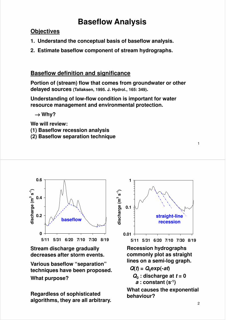
Baseflow AnalysisObjectives

1. Understand the conceptual basis of baseflow analysis.

2. Estimate baseflow component of stream hydrographs.

Baseflow definition and significance

Portion of (stream) flow that comes from groundwater or other

1

Portion of (stream) flow that comes from groundwater or other delayed sources (Tallaksen, 1995. J. Hydrol., 165: 349).

Understanding of low-flow condition is important for water resource management and environmental protection.

→→→→ Why?

We will review:(1) Baseflow recession analysis(2) Baseflow separation technique

0

0.2

0.4

0.6

5/11 5/31 6/20 7/10 7/30 8/19

dis

ch

arg

e (

m3 s

-1)

0.01

0.1

1

5/11 5/31 6/20 7/10 7/30 8/19

dis

ch

arg

e (

m3 s

-1)

straight-line recessionbaseflow

2

5/11 5/31 6/20 7/10 7/30 8/19 5/11 5/31 6/20 7/10 7/30 8/19

Stream discharge gradually decreases after storm events.

Various baseflow “separation” techniques have been proposed.

What purpose?

Regardless of sophisticated algorithms, they are all arbitrary.

Recession hydrographs commonly plot as straight lines on a semi-log graph.

Q(t) = Q0exp(-at)

Q0 : discharge at t = 0a : constant (s-1)

What causes the exponential behaviour?

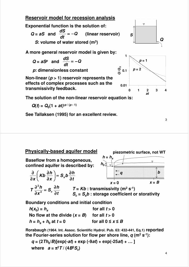
Reservoir model for recession analysis

Exponential function is the solution of:

QSQ

dt

dS−−−−====Q = aS and (linear reservoir)

1

0

p = 1

A more general reservoir model is given by:

Qdt

dS−−−−====Q = aSp and

S: volume of water stored (m3)

3

0.01

0.1

0 1 2 3 4at

Q/Q

0

p = 2

dt

p: dimensionless constant

Non-linear (p > 1) reservoir represents the effects of complex processes such as the transmissivity feedback.

The solution of the non-linear reservoir equation is:

Q(t) = Q0(1 + at)-p / (p - 1)

See Tallaksen (1995) for an excellent review.

b

h0

x = 0 x = B

h = hs

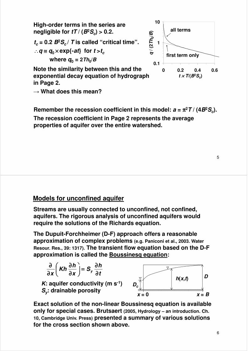
Physically-based aquifer model

Baseflow from a homogeneous, confined aquifer is described by:

t

hbS

x

hKb

xs

∂∂∂∂

∂∂∂∂====

∂∂∂∂

∂∂∂∂

∂∂∂∂

∂∂∂∂

t

hS

x

hT c

∂∂∂∂

∂∂∂∂====

∂∂∂∂

∂∂∂∂2

2

Boundary conditions and initial condition

T = Kb : transmissivity (m2 s-1)Sc = Ssb : storage coefficient or storativity

q

piezometric surface, not WT

4

Boundary conditions and initial condition

h(x0) = hs for all t > 0

No flow at the divide (x = B) for all t > 0

h = hs + h0 at t = 0 for all 0 ≤ x ≤ B

Rorabaugh (1964. Int. Assoc. Scientific Hydrol. Pub. 63: 432-441, Eq.1) reported the Fourier-series solution for flow per shore line, q (m2 s-1):

q = (2Th0/B)[exp(-at) + exp (-9at) + exp(-25at) + … ]

where a = ππππ2T / (4B2Sc)

0.1

1

10

0 0.2 0.4 0.6

q /

(2

Th

0/B

)

t ×××× T/(B2Sc)

all terms

first term only

High-order terms in the series are negligible for tT / (B2Sc) > 0.2.

tc = 0.2 B2Sc / T is called “critical time”.

∴q ≅≅≅≅ q0 ×××× exp{-at} for t >tc

where q0 = 2Th0/B

Note the similarity between this and the exponential decay equation of hydrograph in Page 2.

5

→ What does this mean?

Remember the recession coefficient in this model: a = ππππ2T / (4B2Sc).

The recession coefficient in Page 2 represents the average properties of aquifer over the entire watershed.

Models for unconfined aquifer

Streams are usually connected to unconfined, not confined, aquifers. The rigorous analysis of unconfined aquifers would require the solutions of the Richards equation.

The Dupuit-Forchheimer (D-F) approach offers a reasonable approximation of complex problems (e.g. Paniconi et al., 2003. Water

Resour. Res., 39: 1317). The transient flow equation based on the D-F approximation is called the Boussinesq equation:

hh ∂∂∂∂ ∂∂∂∂∂∂∂∂

6

x = 0 x = B

Dc

Dh(x,t)t

hS

x

hKh

xy

∂∂∂∂

∂∂∂∂====

∂∂∂∂

∂∂∂∂

∂∂∂∂

∂∂∂∂

Exact solution of the non-linear Boussinesq equation is available only for special cases. Brutsaert (2005, Hydrology – an introduction. Ch.

10, Cambridge Univ. Press) presented a summary of various solutions for the cross section shown above.

K: aquifer conductivity (m s-1)Sy: drainable porosity

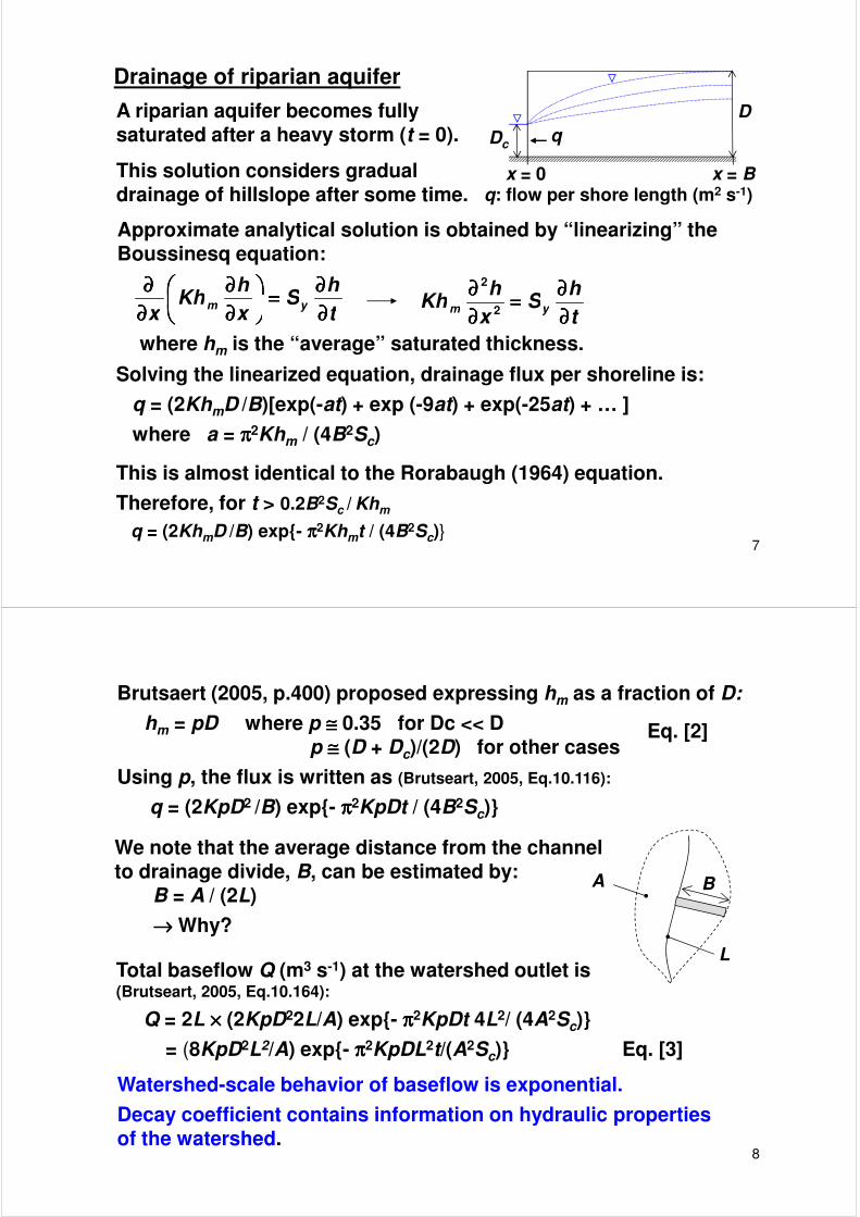
Drainage of riparian aquifer

A riparian aquifer becomes fully saturated after a heavy storm (t = 0).

This solution considers gradual drainage of hillslope after some time.

Approximate analytical solution is obtained by “linearizing” the Boussinesq equation:

t

hS

x

hKh

xym

∂∂∂∂

∂∂∂∂====

∂∂∂∂

∂∂∂∂

∂∂∂∂

∂∂∂∂ hS

hKh ym

∂∂∂∂

∂∂∂∂====

∂∂∂∂

∂∂∂∂2

2

x = 0 x = B

Dc

D

q

q: flow per shore length (m2 s-1)

7

tS

xKh

xym

∂∂∂∂====

∂∂∂∂∂∂∂∂ t

Sx

Kh ym∂∂∂∂

====∂∂∂∂ 2

where hm is the “average” saturated thickness.

Solving the linearized equation, drainage flux per shoreline is:

q = (2KhmD /B)[exp(-at) + exp (-9at) + exp(-25at) + … ]

where a = ππππ2Khm / (4B2Sc)

This is almost identical to the Rorabaugh (1964) equation.

Therefore, for t > 0.2B2Sc / Khm

q = (2KhmD /B) exp{- ππππ2Khmt / (4B2Sc)}

Brutsaert (2005, p.400) proposed expressing hm as a fraction of D:

hm = pD where p ≅≅≅≅ 0.35 for Dc << Dp ≅≅≅≅ (D + Dc)/(2D) for other cases

Using p, the flux is written as (Brutseart, 2005, Eq.10.116):

q = (2KpD2 /B) exp{- ππππ2KpDt / (4B2Sc)}

Eq. [2]

A B

We note that the average distance from the channel to drainage divide, B, can be estimated by:

B = A / (2L)

→→→→

8

Total baseflow Q (m3 s-1) at the watershed outlet is (Brutseart, 2005, Eq.10.164):

Q = 2L ×××× (2KpD22L/A) exp{- ππππ2KpDt 4L2/ (4A2Sc)}

= (8KpD2L2/A) exp{- ππππ2KpDL2t/(A2Sc)} Eq. [3]

L

→→→→ Why?

Watershed-scale behavior of baseflow is exponential.

Decay coefficient contains information on hydraulic properties of the watershed.

0

0.5

1

1.5

5/1 5/21 6/10 6/30 7/20 8/9 8/29 9/18 10/8

Dis

ch

arg

e (m

3s

-1)

2007 20082009 20102011 2012

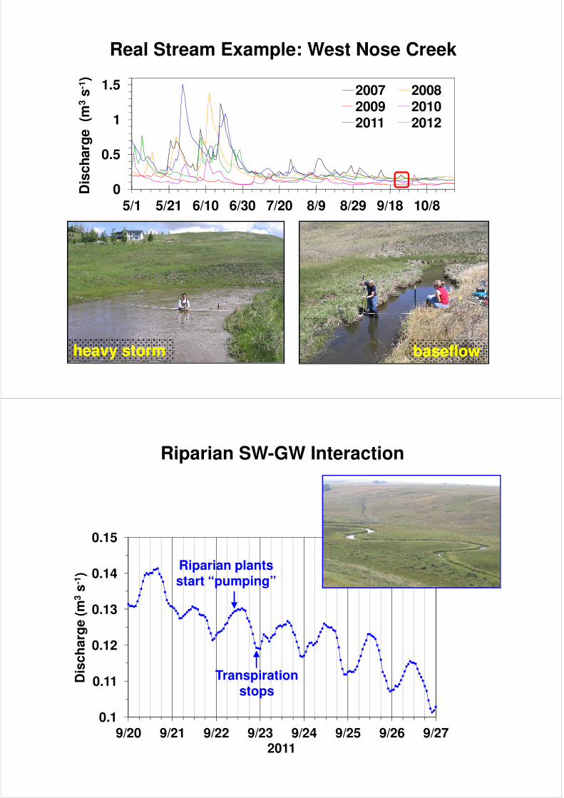
Real Stream Example: West Nose Creek

5/1 5/21 6/10 6/30 7/20 8/9 8/29 9/18 10/8

heavy stormheavy storm baseflowbaseflow

0.14

0.15

3s

-1)

Riparian SW-GW Interaction

Riparian plants start “pumping”

0.1

0.11

0.12

0.13

9/20 9/21 9/22 9/23 9/24 9/25 9/26 9/27

flo

w (

m3/s

)D

isc

ha

rge

(m

3

2011

Transpiration stops

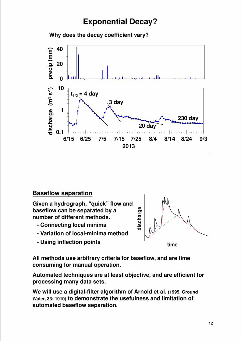
Exponential Decay?

10

0

20

40p

recip

(m

m)

Why does the decay coefficient vary?

11

0.1

1

10

6/15 6/25 7/5 7/15 7/25 8/4 8/14 8/24 9/3

dis

ch

arg

e

(m3

s-1

)

2013

t1/2 = 4 day

3 day

20 day

230 day

Baseflow separation

dis

ch

arg

e

time

Given a hydrograph, “quick” flow and baseflow can be separated by a number of different methods.

- Connecting local minima

- Variation of local-minima method

All methods use arbitrary criteria for baseflow, and are time

- Using inflection points

12

All methods use arbitrary criteria for baseflow, and are time consuming for manual operation.

Automated techniques are at least objective, and are efficient for processing many data sets.

We will use a digital-filter algorithm of Arnold et al. (1995. Ground

Water, 33: 1010) to demonstrate the usefulness and limitation of automated baseflow separation.

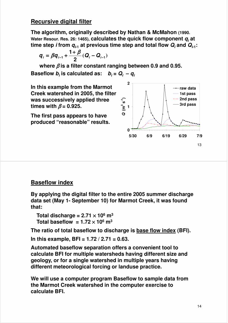
Recursive digital filter

The algorithm, originally described by Nathan & McMahon (1990.

Water Resour. Res. 26: 1465), calculates the quick flow component qi at time step i from qi-1 at previous time step and total flow Qi and Qi-1:

)( 112

1−−−−−−−− −−−−

++++++++==== iiii QQqq

ββββββββ

where ββββ is a filter constant ranging between 0.9 and 0.95.

Baseflow bi is calculated as: bi = Qi – qi

13

0

1

2

5/30 6/9 6/19 6/29 7/9

Q (

m3 s

-1)

raw data

1st pass

2nd pass

3rd pass

In this example from the Marmot Creek watershed in 2005, the filter was successively applied three times with ββββ = 0.925.

The first pass appears to have produced “reasonable” results.

Baseflow index

By applying the digital filter to the entire 2005 summer discharge data set (May 1- September 10) for Marmot Creek, it was found that:

Total discharge = 2.71 ×××× 106 m3

Total baseflow = 1.72 ×××× 106 m3

The ratio of total baseflow to discharge is base flow index (BFI).

In this example, BFI = 1.72 / 2.71 = 0.63.

14

Automated baseflow separation offers a convenient tool to calculate BFI for multiple watersheds having different size and geology, or for a single watershed in multiple years having different meteorological forcing or landuse practice.

We will use a computer program Baseflow to sample data from the Marmot Creek watershed in the computer exercise to calculate BFI.

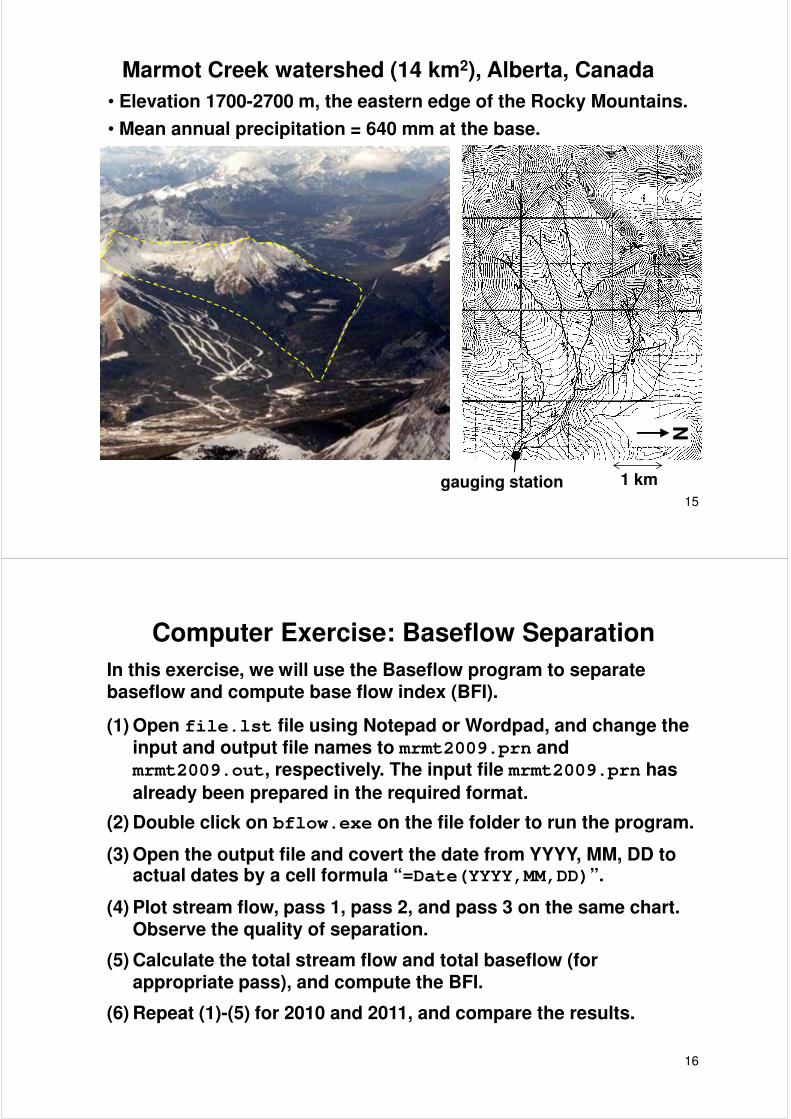
Marmot Creek watershed (14 km2), Alberta, Canada

• Elevation 1700-2700 m, the eastern edge of the Rocky Mountains.

• Mean annual precipitation = 640 mm at the base.

15

gauging station 1 km

N

Computer Exercise: Baseflow Separation

In this exercise, we will use the Baseflow program to separate baseflow and compute base flow index (BFI).

(1) Open file.lst file using Notepad or Wordpad, and change the input and output file names to mrmt2009.prn and mrmt2009.out, respectively. The input file mrmt2009.prn has

already been prepared in the required format.

(2) Double click on bflow.exe on the file folder to run the program.

16

(3) Open the output file and covert the date from YYYY, MM, DD to actual dates by a cell formula “=Date(YYYY,MM,DD)”.

(4) Plot stream flow, pass 1, pass 2, and pass 3 on the same chart. Observe the quality of separation.

(5) Calculate the total stream flow and total baseflow (for appropriate pass), and compute the BFI.

(6) Repeat (1)-(5) for 2010 and 2011, and compare the results.