Embed Size (px)
Citation preview
Basic Biostatistics for Clinicians:How to Use and Interpret Statistics (for the boards)
Elizabeth Garrett-Mayer, PhDAssociate ProfessorDirector of Biostatistics Hollings Cancer Center
Outline for today’s talk
1. Experimental design2. Motivating example3. Types of variables 4. Descriptive statistics5. Population vs. sample6. Confidence intervals7. Hypothesis testing8. Type I and II errors
Experimental Design
How do we set up the study to answer the question?Two main situations
Controlled designsThe experimenter has control“exposure” or “treatments”Randomized clinical trials
Observational designsCohort studiesCase-control studies
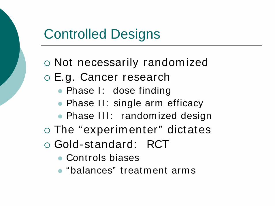
Controlled Designs
Not necessarily randomizedE.g. Cancer research
Phase I: dose findingPhase II: single arm efficacyPhase III: randomized design
The “experimenter” dictatesGold-standard: RCT
Controls biases“balances” treatment arms
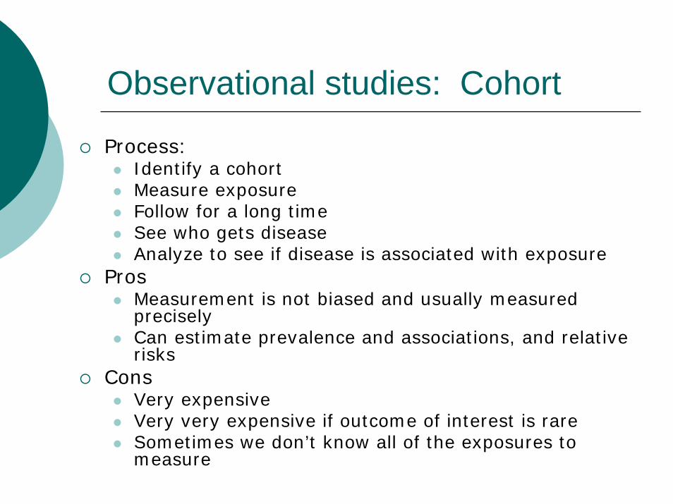
Observational studies: Cohort
Process:Identify a cohortMeasure exposure Follow for a long timeSee who gets diseaseAnalyze to see if disease is associated with exposure
ProsMeasurement is not biased and usually measured preciselyCan estimate prevalence and associations, and relative risks
ConsVery expensiveVery very expensive if outcome of interest is rareSometimes we don’t know all of the exposures to measure
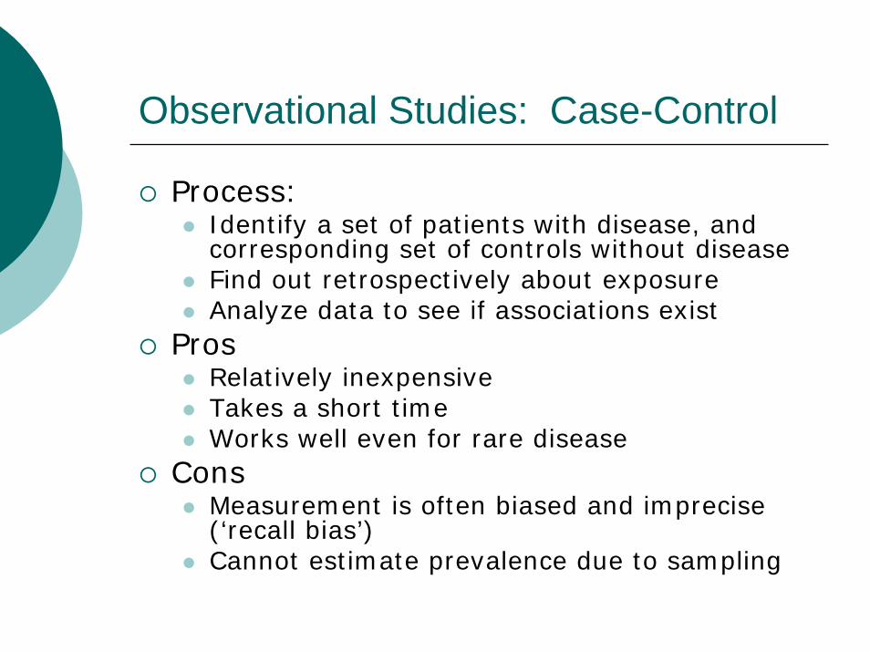
Observational Studies: Case-Control
Process:Identify a set of patients with disease, and corresponding set of controls without diseaseFind out retrospectively about exposureAnalyze data to see if associations exist
ProsRelatively inexpensive Takes a short timeWorks well even for rare disease
ConsMeasurement is often biased and imprecise (‘recall bias’)Cannot estimate prevalence due to sampling
Observational Studies: Why they leave us with questions
• Confounders• Biases
Self-selectionRecall biasSurvival biasEtc.
Motivating example
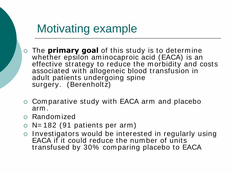
The primary goal of this study is to determine whether epsilon aminocaproic acid (EACA) is an effective strategy to reduce the morbidity and costs associated with allogeneic blood transfusion in adult patients undergoing spine surgery. (Berenholtz)
Comparative study with EACA arm and placebo arm.RandomizedN=182 (91 patients per arm)Investigators would be interested in regularly using EACA if it could reduce the number of units transfused by 30% comparing placebo to EACA
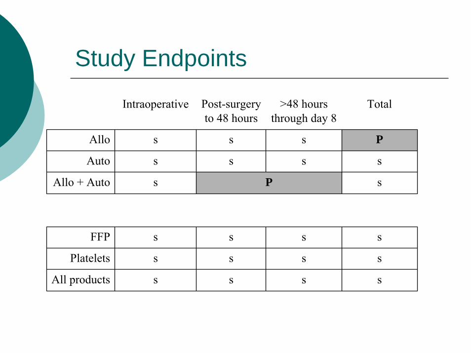
Study Endpoints
Intraoperative Post-surgery to 48 hours
>48 hours through day 8
Total
Allo s s s P
Auto s s s s
Allo + Auto s P s
FFP s s s s
Platelets s s s s
All products s s s s
Three Primary Types of Variables in Medical Research
continuous:blood pressurecholesterolquality of lifeunits of blood
categoricalblood typetransfused/not transfusedcured/not cured
time-to-eventtime to deathtime to progressiontime to immune reconstitutiontime to discharge(?)
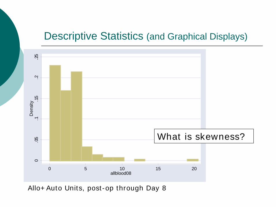
Descriptive Statistics (and Graphical Displays)0
.05
.1.1
5.2
.25
Den
sity
0 5 10 15 20allblood08
What is skewness?
Allo+Auto Units, post-op through Day 8
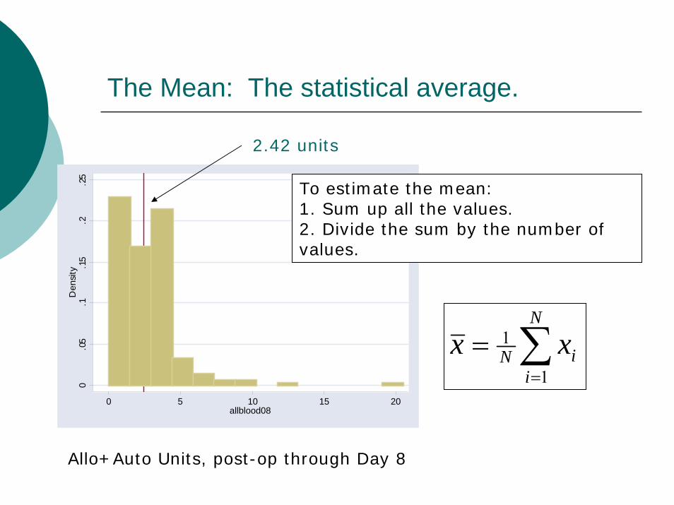
The Mean: The statistical average. 0
.05
.1.1
5.2
.25
Den
sity
0 5 10 15 20allblood08
Allo+Auto Units, post-op through Day 8
To estimate the mean:1. Sum up all the values.2. Divide the sum by the number of values.
2.42 units
∑=
=N
iiN xx
1
1
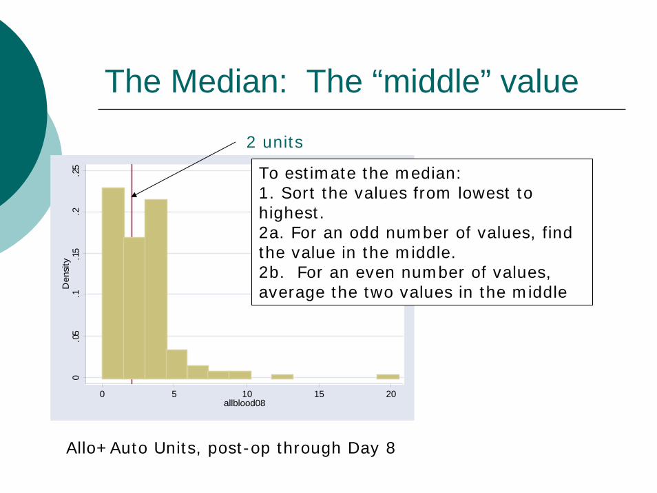
The Median: The “middle” value0
.05
.1.1
5.2
.25
Den
sity
0 5 10 15 20allblood08
To estimate the median:1. Sort the values from lowest to highest.2a. For an odd number of values, find the value in the middle.2b. For an even number of values, average the two values in the middle
2 units
Allo+Auto Units, post-op through Day 8
The mean versus the median
The mean is sensitive to “outliers”The median is not
When the data are highly skewed, the median is usually preferredWhen the data are not skewed, the median and the mean will be very close
0.0
5.1
.15
.2.2
5D
ensi
ty
0 5 10 15 20allblood08
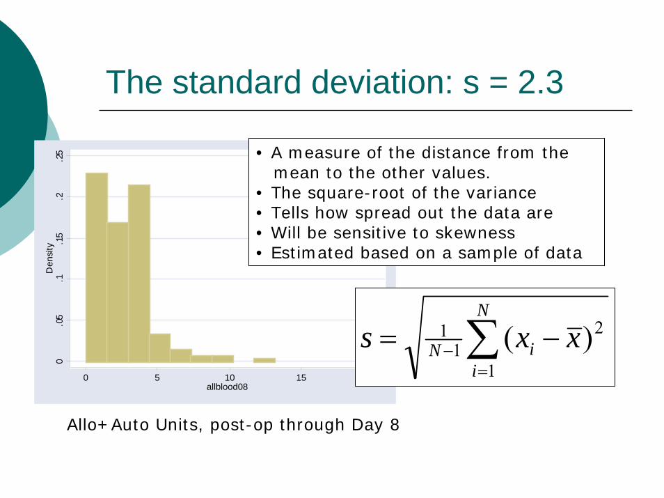
The standard deviation: s = 2.3
• A measure of the distance from the mean to the other values.
• The square-root of the variance• Tells how spread out the data are• Will be sensitive to skewness• Estimated based on a sample of data
2
11
1 )(∑=
− −=N
iiN xxs
Allo+Auto Units, post-op through Day 8
Others
RangeInterquartile rangeModeSkewness
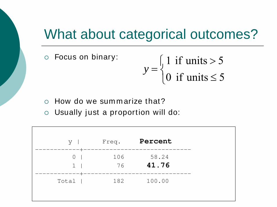
What about categorical outcomes?Focus on binary:
How do we summarize that?Usually just a proportion will do:
⎩⎨⎧
≤>
=5units if 05 units if 1
y
y | Freq. Percent------------+-----------------------------
0 | 106 58.241 | 76 41.76
------------+-----------------------------Total | 182 100.00
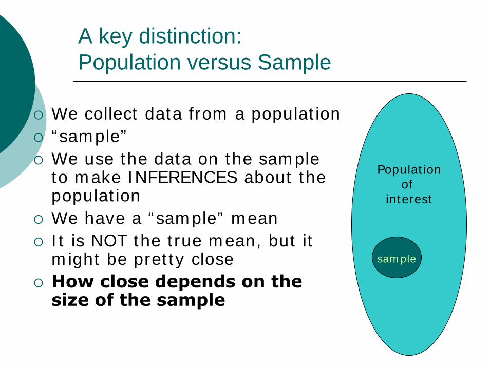
A key distinction: Population versus Sample
We collect data from a population“sample” We use the data on the sample to make INFERENCES about the populationWe have a “sample” meanIt is NOT the true mean, but it might be pretty closeHow close depends on the size of the sample
Populationof
interest
sample
Parameters versus Statistics
A parameter is a population characteristicA statistic is a sample characteristicExample: we estimate the sample mean to tell us about the true population mean
the sample mean is a ‘statistic’the population mean is a ‘parameter’
Statistical Inference
Use the data from the sample to inform us about the population“Generalize”Two common approaches
confidence intervals: tell us likely values for the true population value based on our sample datahypothesis testing: find evidence for or against hypotheses about the population based on sample data
Confidence Intervals
We want to know the true meanAll we have is the sample mean.How close is the sample mean to the true mean?A confidence interval can tell usIt is based on
the sample mean (x)the sample standard deviation (s)the sample size (N)(& the level of confidence)
We usually focus on 95% confidence intervals
Confidence Intervals
What does it mean?It is an interval which contains the TRUE population parameter with 95% certaintyHow do we calculate it?First, we need to learn about the standard error
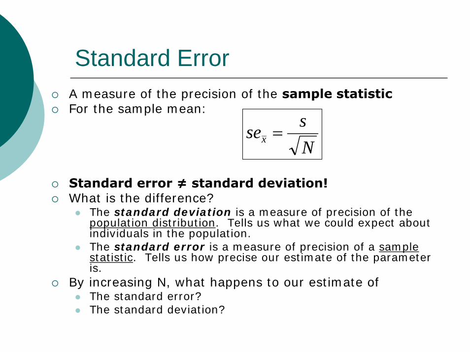
Standard ErrorA measure of the precision of the sample statisticFor the sample mean:
Standard error ≠ standard deviation!What is the difference?
The standard deviation is a measure of precision of the population distribution. Tells us what we could expect about individuals in the population.The standard error is a measure of precision of a sample statistic. Tells us how precise our estimate of the parameter is.
By increasing N, what happens to our estimate ofThe standard error?The standard deviation?
Nssex =
Confidence Intervals
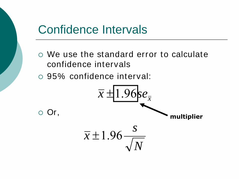
We use the standard error to calculate confidence intervals95% confidence interval:
Or,
xsex 96.1±
Nsx 96.1±
multiplier
What does it mean?
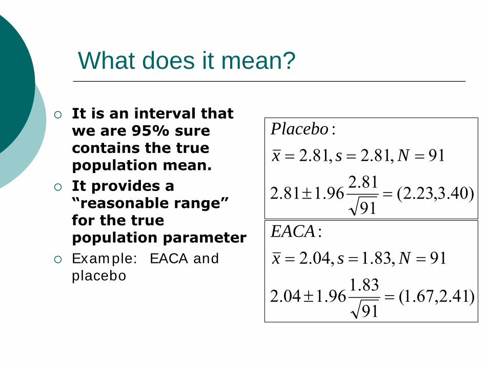
It is an interval that we are 95% sure contains the true population mean.It provides a “reasonable range” for the true population parameterExample: EACA and placebo
)40.3,23.2(9181.296.181.2
91,81.2,81.2:
=±
=== NsxPlacebo
)41.2,67.1(9183.196.104.2
91,83.1,04.2:
=±
=== NsxEACA
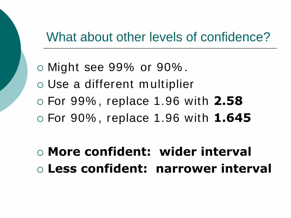
What about other levels of confidence?
Might see 99% or 90%.Use a different multiplierFor 99%, replace 1.96 with 2.58For 90%, replace 1.96 with 1.645
More confident: wider intervalLess confident: narrower interval
Caveats
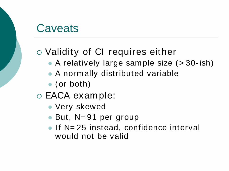
Validity of CI requires eitherA relatively large sample size (>30-ish)A normally distributed variable(or both)
EACA example:Very skewedBut, N=91 per groupIf N=25 instead, confidence interval would not be valid
Caveats
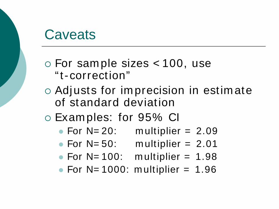
For sample sizes <100, use “t-correction”Adjusts for imprecision in estimate of standard deviationExamples: for 95% CI
For N=20: multiplier = 2.09For N=50: multiplier = 2.01For N=100: multiplier = 1.98For N=1000: multiplier = 1.96
Confidence Intervals
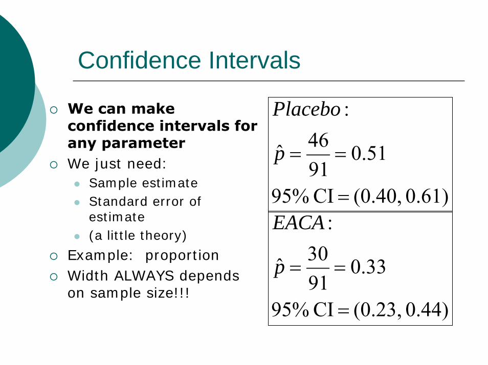
We can make confidence intervals for any parameterWe just need:
Sample estimateStandard error of estimate(a little theory)
Example: proportionWidth ALWAYS depends on sample size!!!
0.61) (0.40, CI %95
51.09146ˆ
:
=
==p
Placebo
0.44) (0.23, CI %95
33.09130ˆ
:
=
==p
EACA
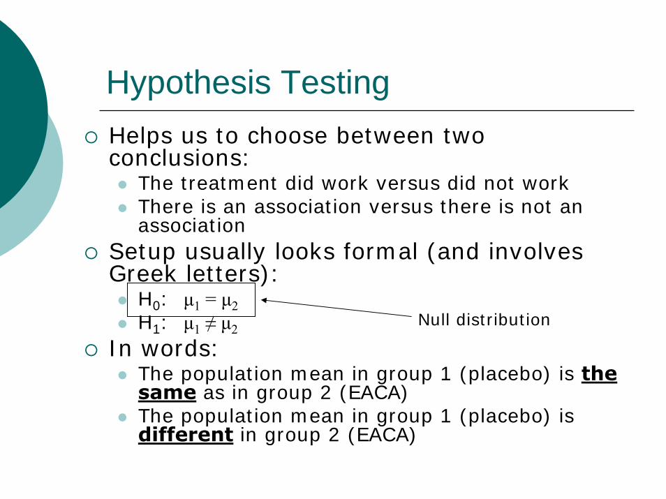
Hypothesis TestingHelps us to choose between two conclusions:
The treatment did work versus did not workThere is an association versus there is not an association
Setup usually looks formal (and involves Greek letters):
H0: μ1 = μ2H1: μ1 ≠ μ2
In words:The population mean in group 1 (placebo) is the same as in group 2 (EACA)The population mean in group 1 (placebo) isdifferent in group 2 (EACA)
Null distribution
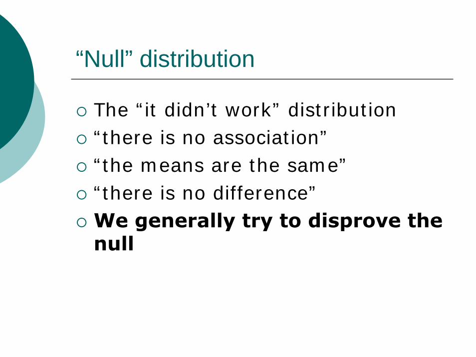
“Null” distribution
The “it didn’t work” distribution“there is no association”“the means are the same”“there is no difference”We generally try to disprove the null
Continuous outcomes: t-test
Several kinds of t-testsTwo sampleone samplePaired
EACA Example: two independent groups → two sample t-testConstruction of test statistic depends on this
Two-sample t-test
No mathematics hereJust know that the following are included:
The means of both groupsThe standard deviations of both groupsThe sample sizes of both groups
Plug it all in the formula and….Out pops a number: the t-statistic
We then compare the t-statistic to the appropriate t-distribution
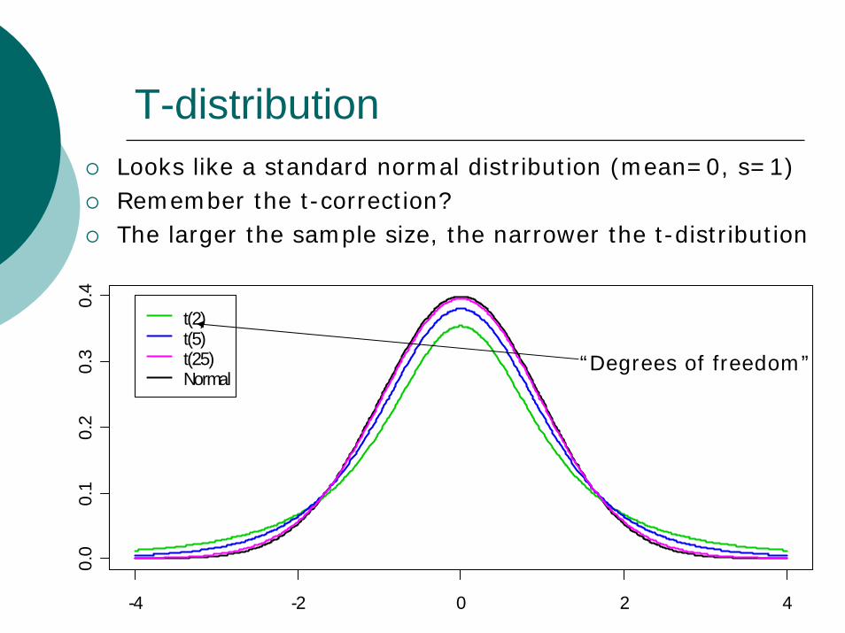
T-distributionLooks like a standard normal distribution (mean=0, s=1)Remember the t-correction?The larger the sample size, the narrower the t-distribution
-4 -2 0 2 4
0.0
0.1
0.2
0.3
0.4
t(2)t(5)t(25)Normal
“Degrees of freedom”
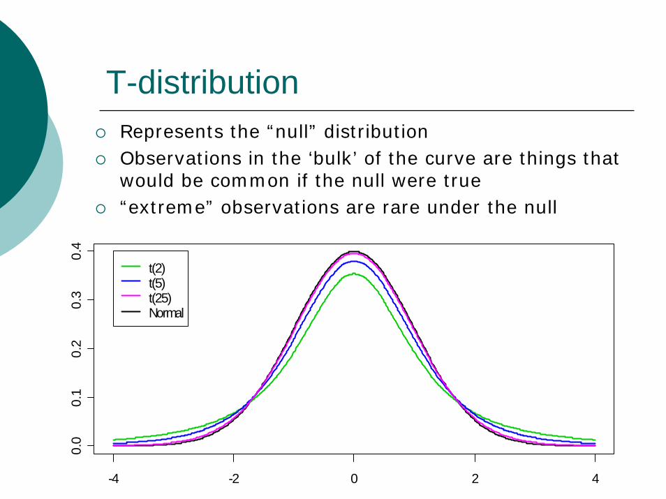
T-distributionRepresents the “null” distributionObservations in the ‘bulk’ of the curve are things that would be common if the null were true“extreme” observations are rare under the null
-4 -2 0 2 4
0.0
0.1
0.2
0.3
0.4
t(2)t(5)t(25)Normal
EACA and placebo
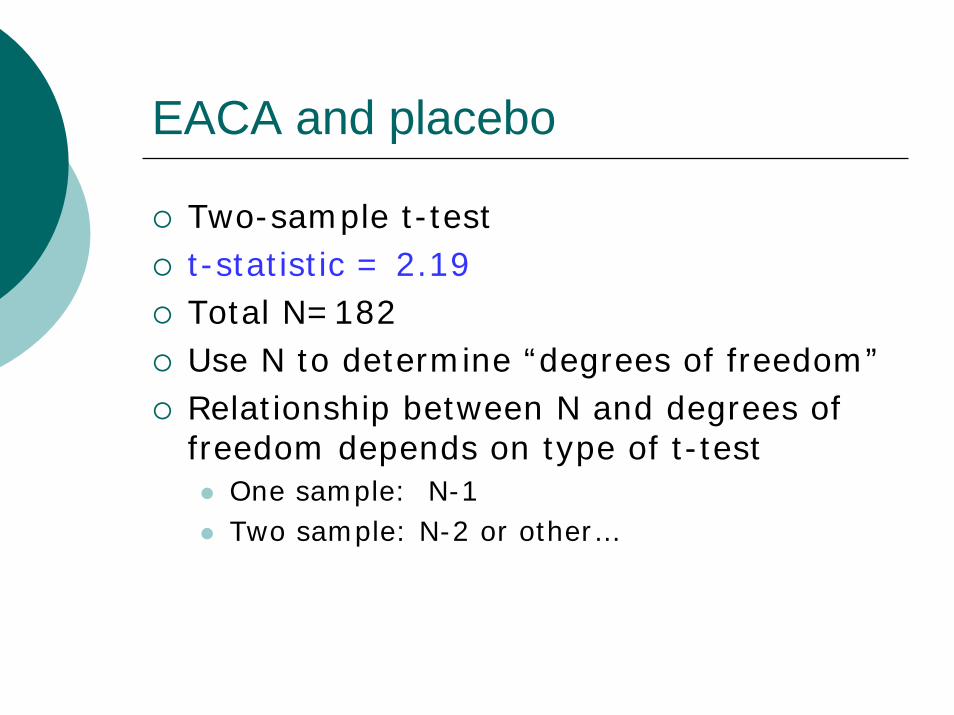
Two-sample t-testt-statistic = 2.19Total N=182Use N to determine “degrees of freedom”Relationship between N and degrees of freedom depends on type of t-test
One sample: N-1Two sample: N-2 or other…
-4 -2 0 2 4
0.0
0.2
0.4 2.19
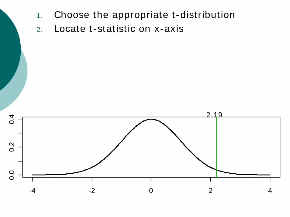
1. Choose the appropriate t-distribution2. Locate t-statistic on x-axis
-4 -2 0 2 4
0.0
0.2
0.4 2.19-2.19
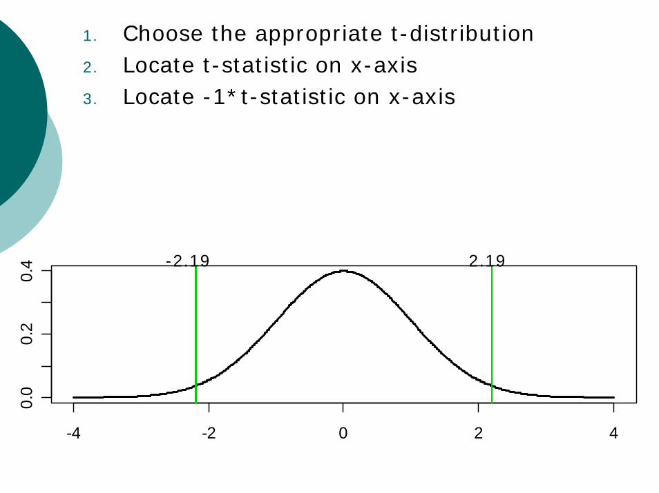
1. Choose the appropriate t-distribution2. Locate t-statistic on x-axis3. Locate -1*t-statistic on x-axis
-4 -2 0 2 4
0.0
0.2
0.4 2.19-2.19
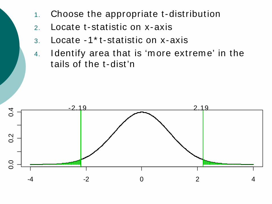
1. Choose the appropriate t-distribution2. Locate t-statistic on x-axis3. Locate -1*t-statistic on x-axis4. Identify area that is ‘more extreme’ in the
tails of the t-dist’n
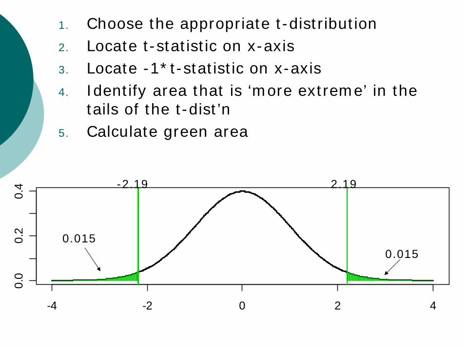
1. Choose the appropriate t-distribution2. Locate t-statistic on x-axis3. Locate -1*t-statistic on x-axis4. Identify area that is ‘more extreme’ in the
tails of the t-dist’n5. Calculate green area
-4 -2 0 2 4
0.0
0.2
0.4 2.19-2.19
0.0150.015
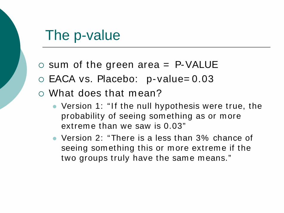
The p-value
sum of the green area = P-VALUEEACA vs. Placebo: p-value=0.03What does that mean?
Version 1: “If the null hypothesis were true, the probability of seeing something as or more extreme than we saw is 0.03”Version 2: “There is a less than 3% chance of seeing something this or more extreme if the two groups truly have the same means.”
The p-value IS NOT
The probability that the null is trueThe probability of seeing the data we sawKey issues to remember:
“…as or more extreme…”“..if the null is true…”Statistic is calculated based on the null distribution!
What about proportions?
T-tests are ONLY for continuous variablesThere are other tests for proportions:
Fisher’s exact testChi-square tests
P-values always mean the same thing regardless of test: the probability of a result as or more extreme under the null hypothesisExample: comparison of proportions
0.50 and 0.33 in placebo and EACAp-value = 0.02
Now what?
What do we do with the p-value?We need to decide if 0.03 is low enough to ‘reject’ the nullGeneral practice:
Reject the null if p<0.05“fail to reject” the null if p>0.05
AD HOC cutoffDEPENDS HEAVILY ON SAMPLE SIZE!!!!!!!!!!!!
Type I error (alpha)
The “significance” cutoffGeneral practice: alpha = 0.05Sometimes:
alpha = 0.10Alpha = 0.01
Why might it differ?Phase of studyHow many hypotheses you are testing
Interpretation of Type I error
The probability of FALSELY rejecting the null hypothesisRecall, 5% of the time, you will get an “extreme” result if the null is truePeople worry a lot about making a type I errorThat is why they set it pretty low (5%)
Type II error
The opposite of type I error“the probability of failing to reject the null when it is true”People don’t worry about this so muchHappens all the timeWhy?Because sample size is too small: not enough evidence to reject the nullHow can we ensure that our sample size is large enough? Power calculations
QUESTIONS???
Contact me:
Other resourcesGlaser: High-Yield BiostatisticsNorman & Streiner: PDQ StatisticsDawson-Saunders & Trapp: Basic Biostatistics
Elizabeth [email protected]