Basic Concepts in Hypothesis Testing*

Rosalind L. P. Phang Department of Mathematics

National University of Singapore

§l. Introduction

Most people make rough confidence statements on many aspects of their daily lives by the choice of an adjective, an adverb, or a phrase. Scientific investigators, industrial engineers and market researchers, among others, often have hypotheses about particular facets of their work areas. These hypotheses need substantiation or verification - or rejection - for one purpose or another. To this end, they gather data and allow them to sup­port or cast doubt on th~ir hypotheses. This process is termed hypothesis testing and is one of two main areas of statistical inference.

Definition : A statistical hypothesis is an assertion or conjecture about the distribution of one or more random variables. If a statistical hypothesis completely specifies the distribution, it is referred to as a simple hypothesis; if not, it is referred to as a composite hypothesis.

§2. General Steps in Hypothesis Testing

The testing of a statistical hypothesis is the application of an explicit set of rules for deciding whether to accept the hypothesis or to reject it. The method of conducting any statistical hypothesis testing can be outlined in six steps :

1. Decide on the null hypothesis H0

The null hypothesis generally expresses the idea of no difference. The symbol we use to denote a null hypothesis is H0 •

2. Decide on the alternative hypothesis H1

The alternative hypothesis, which we denote by H 1 , expresses the idea of some difference. Alternative hypotheses may be one-sided o.r two-sided. Usually the setting of the problem determines the alternative even before the data has been collected.

* Lecture given at the Workshop on Hypothesis Testing and Non-Parametric Statistics for school

teachers, 7 September 1987.

59

3. Calculate the appropriate test statistic

This is a value that we will calculate from the sample data.

4. Decide on the significance level or the critical P-value

All hypothesis testing is liable to errors. There are two basic kinds of error:

• Type I error : Reject H 0 when it is, in fact, true; the probability of committing a type I error is denoted by a.

• Type II error : Reject H 1 when it is, in fact, true; the probability of committing a type II error is denoted by {3.

The objective in all hypothesis testing is to set the Type I error level, also known as the significance level, at a low enough value, and then to use a test statistic which minimises the Type II error level for a given sample size. As we fix the Type I error l.evel, it is best to devise the test in such a way that the Type I error is most serious, in terms of cost.

A critical P -value is the probability that is set by the person doing the test; it is the threshold for the P-value that the tester will use to decide whether the sample is unusual enough, compared to the hypothe­sised population, to indicate that the null hypothesis should be rejected in favour of the alternative.

5. The P-value or critical region of size a

The calculated test statistic is compared to the sampling distribu­tion that the statistic would have if the null hypothesis were true. The comparison is summarised into a probability called a P-value : this is the probability, if the null hypothesis is true, that the statistic would be at least as far from the expected value as it was observed to be in the sample.

The P-value ranges from 0.0 to 1.0. As it approaches 0.0, it indicates that the sample is a rare outcome if the population is as hypothesized. The closer the P-value is to zero, the stronger the evidence against the null hypothesis.

When we are testing the null hypothesis H0 : () = 60 against the two-sided alternative hypothesis H 1 : () =/= ()0 , the critical region consists of both tails of the sampling distribution of the test statistic. Such a test is a two-tailed test. On the other hand, if we are testing the null hypothesis Ho : () = fJo against one-sided alternative H 1 : () < 60 or H 1 : () > 60 , the critical regions are the left tail or right tail of the sampling distribution of the test statistic respectively.

60

6. Statement of conclusion

A decision is made based on the size of the P-value. When the P-value is small (i.e. less than the critical P-value), we reject the null hypothesis. When it is not small (greater than the critical P-value), we accept the null hypothesis.

In the same way, if the value of the test statistic falls in the critical region, we reject the null hypothesis.

The conclusion should, as far as possible, be devoid of statistical terminology. However the significance level should be stated.

The assumption of this test is that the variable is approximately nor­mally distributed. This assumption is less critical the larger the sample size.

In the next section we will explain this hypothesis testing procedure in a variety of situations. The criteria that distinguish between the pro­cedures are :

(a) the statistic used to summarise the sample. This in turn depends on the hypothesis to be tested.

(b) the size of the sample

(c) knowledge about the population before the sampling is done

(d) the number of populations sampled

(e) the number of variables observed

§3. Applications of Hypothesis Testing

In this section, some of the standard tests that are most widely used in applications are presented. All the tests presented are based on normal distribution theory, assuming either that the samples are from normal populations or that they are large enough to justify normal approxima­tions.

3.1 Tests concerning Averages

Suppose we want to test the null hypothesis f.L = f.Lo against one of the alternatives f.L =/= f.Lo , f.L > f.Lo, or f.L < f.Lo on the basis of a random sample

61

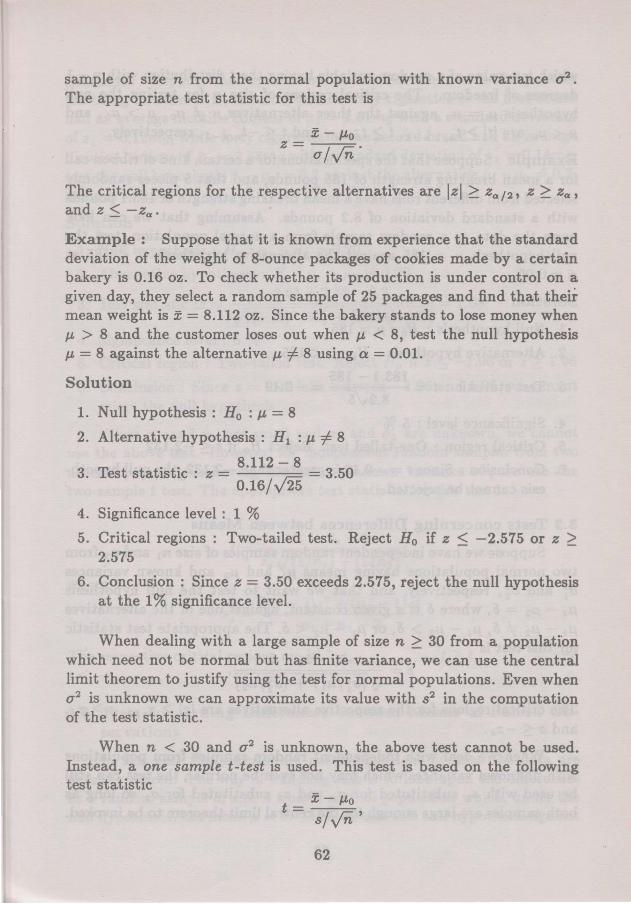
sample of size n from the normal population with known variance u2 •

The appropriate test statistic for this test is

X- JJ.o z= ufvn'

The critical regions for the respective alternatives are lzl ~ Za; 2 , z ~ Za,

and z ~ -Za.

Example : Suppose that it is known from experience that the standard deviation of the weight of 8-ounce packages of cookies made by a certain bakery is 0.16 oz. To check whether its production is under control on a given day, they select a random sample of 25 packages and find that their mean weight is x = 8.112 oz. Since the bakery stands to lose money when p, > 8 and the customer loses out when p, < 8, test the null hypothesis JJ. = 8 against the alternative JJ. =f. 8 using a = 0.01.

Solution

1. Null hypothesis : H0 : p, = 8

2. Alternative hypothesis : H 1 : p, =f. 8

rr . • 8.112-8 3. ~est statistic : z = . ~ = 3.50

0.16/v25

4. Significance level : 1 %

5. Critical regions : Two-tailed test. Reject H0 if z ~ -2.575 or z ~ 2.575

6. Conclusion : Since z = 3.50 exceeds 2.575, reject the null hypothesis at the 1% significance level.

When dealing with a large sample of size n ~ 30 from a populati'on which need not be normal but has finite variance, we can use the central limit theorem to justify using the test for normal populations. Even when u2 is unknown we can approximate its value with s2 in the computation of the test statistic.

When n < 30 and u 2 is unknown, the above test cannot be used. Instead, a one sample t-test is used. This test is based on the following test statistic

X- JJ.o t= sfvn'

62

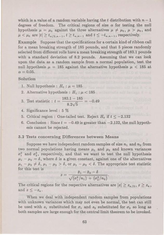
which is a value of a random variable having the t distribution with n -1 degrees of freedom. The critical regions of size a for testing the null hypothesis IL = ILo against the three alternatives IL =/= ILo, IL > ILo, and IL < ILo are itl ~ ta; 2 ,n_ 1 , t ~ ta,n-1 and t ~ -ta,n-1' respectively.

Example Suppose that the specifications for a certain kind of ribbon call for a mean breaking strength of 185 pounds, and that 5 pieces randomly selected from different rolls have a mean breaking strength of 183.1 pounds with a standard deviation of 8.2 pounds. Assuming that we can look upon the data as a random sample from a normal population, test the null hypothesis IL = 185 against the alternative hypothesis IL < 185 at a= 0.05.

Solution

1. Null hypothesis : H 0 : IL = 185

2. Alternative hypothesis : H 1 : IL < 185

. . 183.1- 185 3. Test statistic : t = ~ = -0.49

8.2y5

4. Significance level : 5 % 5. Critical region : One-tailed test. Reject H0 if t ~ -2.132

6. Conclusion: Since t = -0.49 is greater than -2.132, the null hypoth­esis cannot be rejected.

3.2 Tests concerning Differences between Means

Suppose we have independent random samples of size n 1 and n2 from two normal populations having means ILl and IL2 and known variances u~ and u;, respectively, and that we want to test the null hypothesis IL1 - IL2 = o, where o is a given constant, against one of the alternatives IL1 - IL2 =I= o, 1L1 - IL2 > o, or IL1 - IL2 < o. The appropriate test statistic for this test is

The critical regions for the respective alternatives are izl ~ Za ; 2 , z ~ Za,

and z ~ -za.

When we deal with independent random samples from populations with unknown variances which may not even be normal, the test can still be used with s1 substituted for u1 and s2 substituted for u2 so long as both samples are large enough for the central limit theorem to be invoked.

63

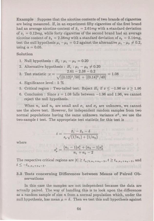
Example Suppose that the nicotine contents of two brands of cigarettes are being measured. If, in an experiment fifty cigarettes of the first brand had an average nicotine content of .X1 = 2.61mg with a standard deviation of s 1 = 0.12mg, while forty cigarettes of the second brand had an average nicotine content of .X2 = 2.38mg with a standard deviation of s2 = 0.14mg, test the null hypothesis p,1 - p,2 = 0.2 against the alternative p,1 - p,2 =/= 0.2, using a = 0.05.

Solution

1. Null hypothesis : H0 : p,1 - p,2 = 0.20

2. Alternative hypothesis : H 1 : p,1 - p,2 =/= 0.20 2.61 - 2.38 - 0.2

3. Test statistic :z = = 1.08 v/[(0.12) 2 /50] + [(0.14) 2 /40]

4. Significance level : 5 % 5. Critical region : Two-tailed test. Reject H0 if z ~ -1.96 or z ~ 1.96

6. Conclusion : Since z = 1.08 falls between -1.96 and 1.96, we cannot reject the null hypothesis.

When n 1 and n 2 are small and u1 and u2 are unknown, we cannot use the above test. However, for independent random samples from two normal populations having the same unknown variance u 2

, we use the two-sample t test. The appropriate test statistic for this test is

where

The respective critical regions are itl ~ ta;2 ,ndn 2 _ 2 , t ~ ta,ndn 2 -2, and t ~ -ta,n 1 +n 2 -2•

3.3 Tests concerning Differences between Means of Paired Ob­servations

In this case the samples are not independent ·because the data are actually paired. The way of handling this is to look upon the differences as a random sample of size n from a normal population which, under the null hypothesis, has mean p, = 6. Then we test this null hypothesis against

64

the appropriate alternative by means of the methods described in Section 3.1. The appropriate test statistic depends on the size of n.

Example An experimenter studied the effect of exposure of lucerne flow­ers to different environmental conditions. He chose 10 vigorous plants with freely exposed flowers at the top and flowers hidden as much as possible at the bottom. Finally he determined the number of seeds set per two pods at each location. The data were :

Plant 1 2 3 4 5 6 7 8 9 10

Top flowers 4.8 5.2 5.7 4.2 4.8 3.9 4.1 3.0 4.6 6.8

Bottom flowers 4.4 3.7 4.7 2.8 4.2 4.3 3.5 3.7 3.1 1.9

Test the hypothesis of no difference between population means against the alternative that top flowers set more seeds for a= 0.05.

Solution The sample of differences (top flowers - bottom flowers) is (0.4, 1.5, 1.0, 1.4, 0.6, -0.4, 0.6, -0.7, 1.5, 4.9). The estimated mean x = 1.08 and standard deviation s = 1.54.

1. Null hypothesis : H0 : p. = 0

2. Alternative hypothesis : H 1 : p. > 0

3. Test statistic : t = l.08 ~ = 2.22

1.54/ 10

4. Significance level : 5 % 5. Critical region : One-tailed test. Reject H0 if t ~ 2.132

6. Conclusion : Since t = 2.22 is greater than 2.132, the null hypothesis cannot be rejected.

References

[1] J.E. Freund & R.E. Walpole, Mathematical Statistics, (4th edition), Prentice-Hall International, 1987.

[2] E.L. Lehman, Testing Statistical Hypotheses, John Wiley, 1959.

[3] A.M. Mood, F .A. Graybill & D.C. Boes, Introduction to the Theory of Statistics, (3rd edition), McGraw Hill, 1974.

65