Embed Size (px)
Citation preview
Massachusetts Institute of Technology Course Notes 86.042J/18.062J, Fall ’02: Mathematics for Computer ScienceProfessor Albert Meyer and Dr. Radhika Nagpal
Basic Counting, Pigeonholing, Permutations
1 Counting by Matching
Counting is a theme throughout discrete mathematics: how many leaves in a tree, minimal colorings of a graph, trees with a given set of vertices, five-card hands in a deck of fifty-two, consistent rankings of players in a tournament, stable marriages given boy’s and girl’s preferences, and so on.
A good way to count things is to match up things to be counted with other things that we know how to count. We saw an example of this early in the term when we counted the size of a powerset of a set of size n by finding an exact matching between elements of the powerset and the 2n binary strings of length n.
The matching doesn’t have to be exact, i.e., a bijection, to be informative. For example, suppose we want to determine the cardinality of the set of watches in the 6.042 classroom on a typical day. The set of watches can be correlated with the set of people in the room; specifically, for each person there is at most one watch (at least, let’s assume this). Now we know something about the cardinality of the set of students, since there are only 146 people signed up for 6.042. There are also three lecturers and eight TA’s, and these would typically be the only nonstudents in the room. So we can conclude that there are at most 157 watches in the classroom on a typical day.
This type of argument is very simple, but also quite powerful. We will see how to use such simple arguments to prove results that are hard to obtain any other way.
2 Matchings as Bijections
The “matching up” we talked about more precisely refers to finding injections, surjections, and bijections between things we want to count and things to be counted. The following Theorem formally justifies this kind of counting:
Theorem 2.1. Let A and B be finite sets and f : from A to B be a function. If
1. f is a bijection, then |A| = |B|,
2. f is an injection, then |A| ≤ |B|,
3. f is a surjection, then |A| ≥ |B|.
Copyright © 2002, Prof. Albert R. Meyer.
2 Course Notes 8: Basic Counting, Pigeonholing, Permutations
This is one of those theorems that is so fundamental that it’s not clear what simpler axioms are appropriate to use in proving it. In fact, we can’t prove it yet, because we haven’t defined the concept that it’s all about, namely, the size or cardinality, |A|, of a finite set, A. Intuitively, a set, A, has n elements if it equals {a1, a2, . . . , an} where the ai are all different. Now ellipsis is dangerous, so we should avoid it in a definition this basic. What is the notation “a1, a2, . . . , an ” intended to convey? It means that there is a first element, a1, and a second element, a2, and in general, given any i ≤ n, there is an ith element ai. Also, all the ai’s for different i’s are different. This explains how we arrive at a rigorous definition:
Definition 2.2. A set A has cardinality n ∈ N, in symbols, |A| = n, iff there is a bijection from {1, 2, . . . , n} to A. The special case when n = 0 is that |∅| = 0. A set is finite iff it has cardinality n for some n ∈ N.
With this definition, we could prove Theorem 2.1 by appeal to basic properties of functions and natural numbers. For example, if f : A to B is a bijection, and |A| = n, then we can prove that |B| = n as follows: since |A| = n, there is a bijection g : {1, 2, . . . , n} to A. Then f ◦ g is a bijection from {1, 2, . . . , n} to B, so by definition, |B| = n.
Here we used the fact that the composition of bijections is a bijection. This fact itself follows just from the logical properties of equality and the definition of a bijection; it does not even depend on any properties of numbers. So we can say that we proved part 1 of Theorem 2.1 from more fundamental mathematical concepts. The other two parts can be proved using similar properties of functions along with ordinary induction, but we’ll skip them: the proofs are exercises in formal logic that are not very informative about counting.
Notice that the condition in Theorem 2.1 that A and B are finite sets is important. It’s not even clear what the size of an infinite set ought to be, or whether it’s possible for one infinite set to be “larger” than another. We’ll avoid this issue in these notes by only counting the sizes of finite sets.
2.1 Counting Functions
The bijection between length n binary strings and a powerset can be generalized to help in counting the number of functions from one set to another:
Question: How many different functions are there from finite set A to finite set B?
Theorem 2.3. If A and B are finite sets, with |A| = n and |B| = m, then the cardinality of the set of functions from A to B is mn .
Proof. We will use a bijection from {f | f : A → B} to {s | s is a length n string of elements from B}. The mapping is f �→ sf where sf ::= f (a1)f (a2) · · · f (an), i.e., the value of the ith position in sf is equal to f (ai).
We will prove that this mapping is a bijection. First we prove that the mapping is injective (one-to-one) by contradiction. Suppose that f �= g and sf = sg . But f �= g implies that there exists an i ∈ N, where 1 ≤ i ≤ n, we have f (ai) �= g(ai). But that implies that the ith position in sf and sg
are different, which is a contradiction.
Next we prove that the mapping is surjective (onto), i.e., that every length n string, s, of elements from B equals sf for some function f : A → B. Denote the ith position in such a string, s, by s[i].
Course Notes 8: Basic Counting, Pigeonholing, Permutations 3
Now define a function f by the rule that f (ai) ::= s[i], for 1 ≤ i ≤ n. This defines the required f : A → B such that sf = s.
Since this mapping is a bijection, we know that the number of functions from A to B is equal to the number of strings of length n from the elements of B. In section 5 we will see that the number of such strings is mn by the Product Rule.
3 The Pigeonhole Principle
Theorem 2.1 part 2 tells us that if there is an injection from A to B, then |A| ≤ |B|. The contra-positive of this statement is that if |A| > |B|, and f is a function from A to B, then f is not an injection.
Corollary 3.1. Let A and B be finite sets. If |A| > |B| and f : A → B, then there exist distinct elements a and a� in A such that f (a) = f (a�).
This Corollary is known as the Pigeonhole Principle because it can be paraphrased as:
The Pigeonhole Principle: If there are more pigeons than pigeonholes, then there must be at least two pigeons in one hole.
Proof. Let A be the set of “pigeons”, let B be the set of “holes”, and let the function f : A → B define the assignment of pigeons to holes. Since |A| > |B|, Corollary 3.1 implies that there exist two distinct pigeons, a �= a� , assigned to the same hole, f (a).
As a trivial application of the Pigeonhole Principle, suppose that there are three people in a room. The pigeonhole principle implies that two have the same gender. In this case, the “pigeons” are the three people and the “pigeonholes” are the two possible genders, male and female. Since there are more pigeons than holes, two pigeons must be in the same pigeonhole; that is, two people must have the same gender.
Claim 3.2. In New York (City) there live at least two people with the same number of hairs.
Proof (found on the web). I ran experiments with members of my family. My teenage son secured himself the highest marks sporting, in my estimate, about 900 hairs per square inch. Even assuming a pathological case of a 6 feet (two-sided) fellow 50 inch across, covered with hair head, neck, shoulders and so on down to the toes, the fellow would have somewhere in the vicinity of 7,000,000 hairs which is probably a very gross over-estimate to start with. The Hammond’s World Atlas I purchased some 15 years ago, estimates the population of the New York City between 7,500,000 and 9,000,000. The assertion therefore follows from the pigeonhole principle.
The pigeonhole principle seems too obvious to be really useful, but the next two examples show how it gives short proofs of results that are difficult to obtain by other means.
4 Course Notes 8: Basic Counting, Pigeonholing, Permutations
3.1 Pigeonhole Principle Example: A Final Exam Question
A problem on an old final exam was to prove the following claim:
Claim. In every set of 1000 integers, there are two integers x and y such that 573 | (x − y).
At first glance, this looks very hard! Those 1000 numbers could be anything! Since there are no less than 1000 integer-valued variables here, even our old standby, induction, seems hopeless. Surprisingly, however, there is a short proof using the Pigeonhole Principle.
To apply the Pigeonhole Principle, we must identify two things: pigeons and holes. Furthermore, to prove anything with the Pigeonhole Principle, we must have more pigeons than holes. Since there are only two numbers mentioned in this problem, a natural thing to try is 1000 pigeons and 573 holes.
Under this interpretation, a pigeon is an integer, but what is a hole? Ideally, the existence of two pigeons and in the same hole should be equivalent to the existence of two numbers x and y such that 573 | (x − y). This suggests numbering the holes 0, 1, . . . 572 and putting in hole n all integers congruent to n modulo 573. Now we can construct a proof:
Proof. Let S be a set of 1000 integers. Let M = {0, 1, . . . 572}. Let f from S to M be the function defined by f (n) = n mod 573. Since |S| > |M |, Corollary 3.1 implies that there exist distinct elements x and y in S such that f (x) = f (y). This means (x mod 573) = (y mod 573) and so 573 | (x − y).
Really there was nothing special about the numbers 1000 and 573 other than the fact that 1000 > 573. We could have made a stronger claim: if n > m, then in every set of n integers, there are two integers x and y such that m | (x − y).
3.2 Example: Subsets of a List of Numbers
Show that any given 10 distinct positive numbers less than 100, that two completely different subsets sum to the same quantity.
The numbers all vary between 1 and 99. Therefore the maximum sum of any 10 chosen numbers is 90+91+92+ . . . 99 = 945. The number of different subsets of the 10 numbers is 210 − 1 (excluding the null set) = 1023. We have 1023 pigeons and 945 holes. Using the pigeonhole principle, we can argue that two different subsets map to the same sum. If these subsets have a common number or numbers, we can always remove the common numbers to produce two completely different subsets that sum to the same quantity.
3.3 20 Questions and Binary Search
Here is a game. I think of an animal. You can ask me 20 questions that take a yes/no answer such as, “Is the animal bigger than a breadbox?” To win the game, you must ask a question like, “Is the animal a walrus?” or “Is the animal a zebra?” and receive a “yes” answer. In effect, you have 19 questions to determine which animal I am thinking of, and then you must use 1 question to confirm your guess.
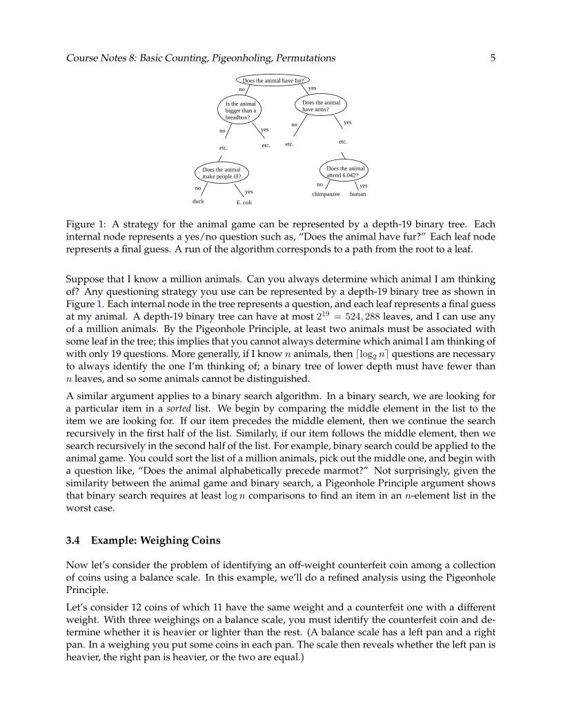
Course Notes 8: Basic Counting, Pigeonholing, Permutations 5
Does the animal have fur?
Is the animalbigger than abreadbox?
Does the animalhave arms?
Does the animalattend 6.042?
humanchimpanzee
Does the animalmake people ill?
duck E. coli
etc. etc.etc.etc.
yes
yes
yesyes
yes
no
no
nono
no
Figure 1: A strategy for the animal game can be represented by a depth-19 binary tree. Each internal node represents a yes/no question such as, “Does the animal have fur?” Each leaf node represents a final guess. A run of the algorithm corresponds to a path from the root to a leaf.
Suppose that I know a million animals. Can you always determine which animal I am thinking of? Any questioning strategy you use can be represented by a depth-19 binary tree as shown in Figure 1. Each internal node in the tree represents a question, and each leaf represents a final guess at my animal. A depth-19 binary tree can have at most 219 = 524, 288 leaves, and I can use any of a million animals. By the Pigeonhole Principle, at least two animals must be associated with some leaf in the tree; this implies that you cannot always determine which animal I am thinking of with only 19 questions. More generally, if I know n animals, then �log2 n� questions are necessary to always identify the one I’m thinking of; a binary tree of lower depth must have fewer than n leaves, and so some animals cannot be distinguished.
A similar argument applies to a binary search algorithm. In a binary search, we are looking for a particular item in a sorted list. We begin by comparing the middle element in the list to the item we are looking for. If our item precedes the middle element, then we continue the search recursively in the first half of the list. Similarly, if our item follows the middle element, then we search recursively in the second half of the list. For example, binary search could be applied to the animal game. You could sort the list of a million animals, pick out the middle one, and begin with a question like, “Does the animal alphabetically precede marmot?” Not surprisingly, given the similarity between the animal game and binary search, a Pigeonhole Principle argument shows that binary search requires at least log n comparisons to find an item in an n-element list in the worst case.
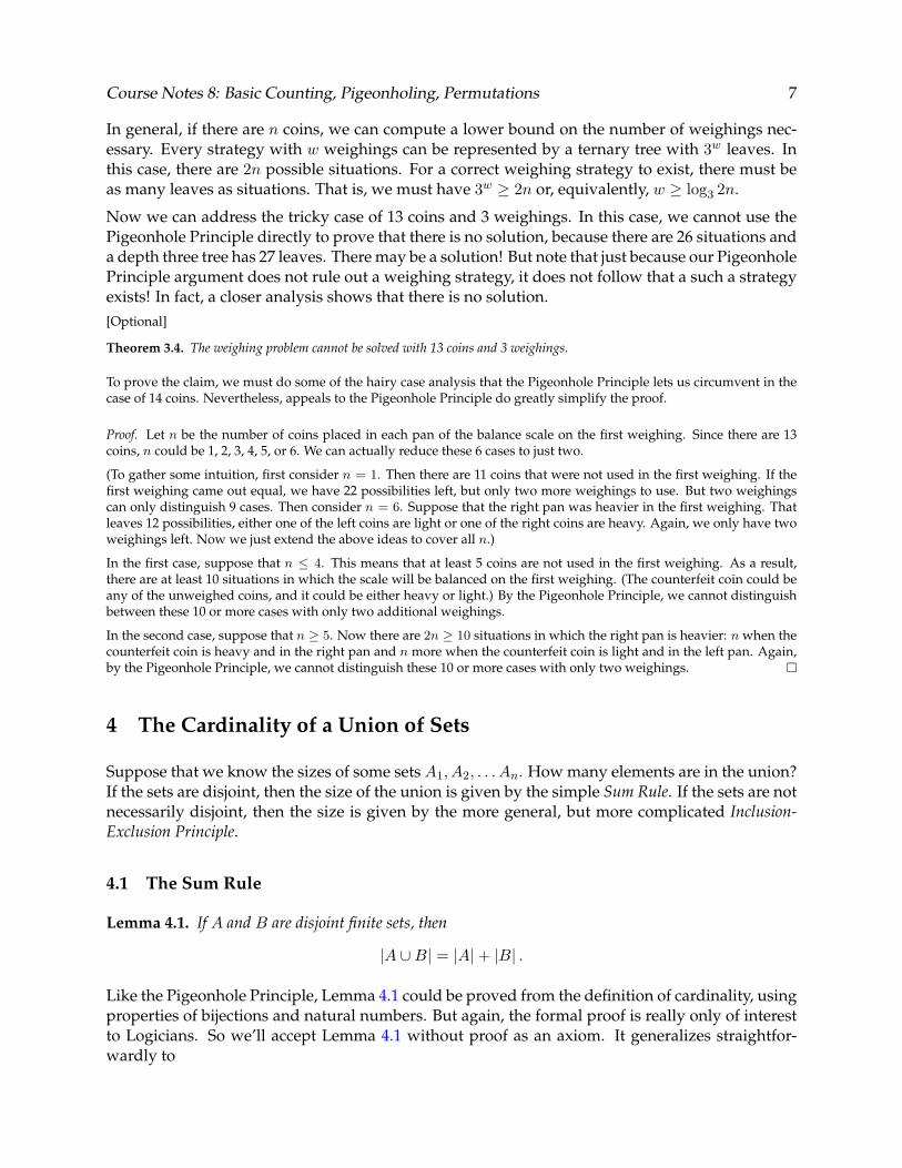
3.4 Example: Weighing Coins
Now let’s consider the problem of identifying an off-weight counterfeit coin among a collection of coins using a balance scale. In this example, we’ll do a refined analysis using the Pigeonhole Principle.
Let’s consider 12 coins of which 11 have the same weight and a counterfeit one with a different weight. With three weighings on a balance scale, you must identify the counterfeit coin and determine whether it is heavier or lighter than the rest. (A balance scale has a left pan and a right pan. In a weighing you put some coins in each pan. The scale then reveals whether the left pan is heavier, the right pan is heavier, or the two are equal.)

6 Course Notes 8: Basic Counting, Pigeonholing, Permutations
b b b b vs. b b b b2 3 41 5 6 7 8
b b b vs. b b b1 2 3 9 10 11
b vs. b9 10
heavyb is
heavyb is
911b is10
<
<
<=
=
=
=
<
>
>
>
>
>=<
heavy
Figure 2: A strategy for the weighing problem can be represented by a ternary tree. Each internal node represents a weighing. Each leaf node represents a result. A run of the algorithm corresponds to a path from the root to a leaf. At each internal node, we perform the weighing associated with the node and descend to a child based on the result. At a leaf, we output the indicated result.
The problem is solvable using a tricky algorithm represented by a ternary tree as shown in Figure 2. Each internal node in the tree represents a weighing such as, “put coins 1, 3, and 5 on one side and 2, 8, and 10 on the other side”. Each leaf node represents a result such as, “the 11th coin is heavier than the rest”. A run of the algorithm corresponds to a path from the root to a leaf. At each internal node, we perform the weighing associated with the node. Based on the result, we descend to one of the three children. When we reach a leaf, we output the indicated result.
Suppose that we wanted to solve the same problem with more coins, but still with only three weighings. The case with 13 coins is complicated and we’ll put it off a bit. However, if there are 14 coins, then we can prove that no solution exists. This would seem to require an elaborate case analysis to rule out every possible strategy. Actually, we can use the Pigeonhole Principle to give a short proof that no weighing strategy exists for 14 coins.
Theorem 3.3. The weighing problem cannot be solved with 14 coins and 3 weighings.
Proof. The pigeons are the possible situations. Since any one of the 14 coins could be the counterfeit one and the counterfeit coin could be either heavier or lighter than the rest, there are 28 possible situations and so 28 pigeons. The holes are the 27 leaves of the depth-3 ternary tree used to represent the weighing strategy. Since there are more pigeons than holes, the Pigeonhole Principle implies that some hole must have two pigeons; that is, some leaf is not associated with a unique situation. Therefore, for every weighing strategy, there is some pair of situations that the strategy cannot distinguish. In at least one of these situations, the strategy must give the wrong answer.
What if we had four weighings—could we identify the counterfeit coin from among 41? In this case, there are 2 · 41 = 82 possible situations or pigeons. Every four-weighing strategy can be represented by a depth four ternary tree with 34 = 81 leaves or pigeonholes. Once again, the Pigeonhole Principle implies that in every weighing strategy, some leaf of the tree must be associated with two or more situations. The strategy cannot distinguish these situations and so must sometimes give the wrong answer.
Course Notes 8: Basic Counting, Pigeonholing, Permutations 7
In general, if there are n coins, we can compute a lower bound on the number of weighings necessary. Every strategy with w weighings can be represented by a ternary tree with 3w leaves. In this case, there are 2n possible situations. For a correct weighing strategy to exist, there must be as many leaves as situations. That is, we must have 3w ≥ 2n or, equivalently, w ≥ log3 2n.
Now we can address the tricky case of 13 coins and 3 weighings. In this case, we cannot use the Pigeonhole Principle directly to prove that there is no solution, because there are 26 situations and a depth three tree has 27 leaves. There may be a solution! But note that just because our Pigeonhole Principle argument does not rule out a weighing strategy, it does not follow that a such a strategy exists! In fact, a closer analysis shows that there is no solution. [Optional]
Theorem 3.4. The weighing problem cannot be solved with 13 coins and 3 weighings.
To prove the claim, we must do some of the hairy case analysis that the Pigeonhole Principle lets us circumvent in the case of 14 coins. Nevertheless, appeals to the Pigeonhole Principle do greatly simplify the proof.
Proof. Let n be the number of coins placed in each pan of the balance scale on the first weighing. Since there are 13 coins, n could be 1, 2, 3, 4, 5, or 6. We can actually reduce these 6 cases to just two.
(To gather some intuition, first consider n = 1. Then there are 11 coins that were not used in the first weighing. If the first weighing came out equal, we have 22 possibilities left, but only two more weighings to use. But two weighings can only distinguish 9 cases. Then consider n = 6. Suppose that the right pan was heavier in the first weighing. That leaves 12 possibilities, either one of the left coins are light or one of the right coins are heavy. Again, we only have two weighings left. Now we just extend the above ideas to cover all n.)
In the first case, suppose that n ≤ 4. This means that at least 5 coins are not used in the first weighing. As a result, there are at least 10 situations in which the scale will be balanced on the first weighing. (The counterfeit coin could be any of the unweighed coins, and it could be either heavy or light.) By the Pigeonhole Principle, we cannot distinguish between these 10 or more cases with only two additional weighings.
In the second case, suppose that n ≥ 5. Now there are 2n ≥ 10 situations in which the right pan is heavier: n when the counterfeit coin is heavy and in the right pan and n more when the counterfeit coin is light and in the left pan. Again, by the Pigeonhole Principle, we cannot distinguish these 10 or more cases with only two weighings.
4 The Cardinality of a Union of Sets
Suppose that we know the sizes of some sets A1, A2, . . . An. How many elements are in the union? If the sets are disjoint, then the size of the union is given by the simple Sum Rule. If the sets are not necessarily disjoint, then the size is given by the more general, but more complicated Inclusion-Exclusion Principle.
4.1 The Sum Rule
Lemma 4.1. If A and B are disjoint finite sets, then
|A ∪ B| = |A| + |B| .
Like the Pigeonhole Principle, Lemma 4.1 could be proved from the definition of cardinality, using properties of bijections and natural numbers. But again, the formal proof is really only of interest to Logicians. So we’ll accept Lemma 4.1 without proof as an axiom. It generalizes straightforwardly to
8 Course Notes 8: Basic Counting, Pigeonholing, Permutations
Theorem 4.2 (Sum Rule). If A1, A2, . . . An are disjoint sets, then:
|A1 ∪ A2 ∪ . . . ∪ An| = |A1| + |A2| + . . . + |An|.
The Sum Rule says that the number of elements in a union of disjoint sets is equal to the sum of the sizes of all the sets. The Sum Rule can be proved from Lemma 4.1 by induction on the number of sets.
As an example use of the Sum Rule, suppose that MIT graduates 60 majors in math, 200 majors in EECS, and 40 majors in physics. How many students graduate from MIT in these three departments? Let A1 be the set of math majors, A2 be the set of EECS majors, and A3 be the set of physics majors. The set of graduating students in these three departments is A1 ∪ A2 ∪ A3. Assume for now that these sets are disjoint; that is, there are no double or triple majors. Then we can apply the Sum Rule to determine the total number of graduating students.
|A1 ∪ A2 ∪ A3| = |A1| + |A2| + |A3| = 60 + 200 + 40
= 300
4.2 Inclusion-Exclusion Principle (special cases)
The Sum Rule gives the cardinality of a union of disjoint sets. The Inclusion-Exclusion Principle gives the cardinality of a union of sets that may intersect. The Inclusion-Exclusion Principle for n sets is messy to write down, so we’ll start with the simple special cases n = 2 and n = 3.
Theorem 4.3 (Inclusion-Exclusion Principle for 2 sets). Let A and B be sets, not necessarily disjoint.
|A ∪ B| = |A| + |B| − |A ∩ B|
Here’s a standard proof you’ll find in many texts, including Rosen (p. 47):
Proof. Items in the union of A and B that are in the intersection of A and B are counted twice in the sum |A| + |B|. Therefore, by subtracting |A ∩ B|, every element is counted once overall.
Here’s how to prove it without handwaving about “counting twice.”
Lemma 4.4. For any finite set, B, and set, A,
|A ∩ B| + |B − A| = |B| .
Proof. The definitions of intersection and set difference imply that
(A ∩ B) ∪ (B − A) = B,
and that A ∩ B and B − A are disjoint. So Lemma 4.4 follows immediately by substituting A ∩ B for A and B − A for B in Lemma 4.1.
Course Notes 8: Basic Counting, Pigeonholing, Permutations 9
But now we can observe that A ∪ B = A ∪ (B − A), and A and B − A are disjoint, so
|A ∪ B| = |A| + |B − A| by Lemma 4.1 = |A| + (|B| − |A ∩ B|) by Lemma 4.4 = |A| + |B| − |A ∩ B| .
Theorem 4.5 (Inclusion-Exclusion Principle for 3 sets). Let A, B, and C be sets, not necessarily disjoint.
|A ∪ B ∪ C| = |A| + |B| + |C| − |A ∩ B| − |A ∩ C| − |B ∩ C|+ |A ∩ B ∩ C|
Though this formula contains many terms, the general pattern is easy to remember: add the sizes of individual sets (first line), subtract intersections of pairs of sets (second line), and add the inter-section of all three sets (third line).
Proof. Items contained in just one of the sets A, B, or C are counted once on the first line. Since these items are not contained in any intersection of sets, they are not subtracted away on the second line or counted again on the third line. In total, these items are counted just once.
Items contained in exactly two of the sets A, B, and C (not in all three) are counted twice on the first line, subtracted away once on the second line, and not counted again on the third line. Again, in total, these items are counted just once.
Items contained in all three sets A, B, and C are counted three times on the first line, subtracted away three times on the second line, and added back once on the third line. Since 3 − 3 + 1 = 1, these items are also counted just once overall.
The name “Inclusion-Exclusion” comes from the way items are counted, subtracted away, counted again, etc.
Earlier we applied the Sum Rule to count MIT graduates in math, EECS, and physics, assuming that there were no double or triple majors. Using Inclusion-Exclusion, we can count the number of graduates even if some people have multiple majors. (After all, this is MIT, where some students even have 4 majors...) Suppose the numbers are as follows:
60 200 40 10 4 15 2
math majorsEECS majorsphysics majorsmath/EECS double majorsmath/physics double majorsEECS/physics double majorstriple majors
(|A| = 60)(|B| = 200)(|C| = 40)(|A ∩ B| = 10)(|A ∩ C| = 4)(|B ∩ C| = 15)(|A ∩ B ∩ C| = 2)
� � �
� � �
� �
� �
10 Course Notes 8: Basic Counting, Pigeonholing, Permutations
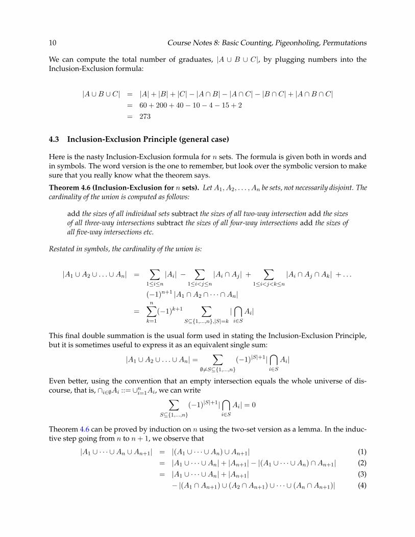
We can compute the total number of graduates, |A ∪ B ∪ C|, by plugging numbers into the Inclusion-Exclusion formula:
|A ∪ B ∪ C| = |A| + |B| + |C| − |A ∩ B| − |A ∩ C| − |B ∩ C| + |A ∩ B ∩ C| = 60 + 200 + 40 − 10 − 4 − 15 + 2
= 273
4.3 Inclusion-Exclusion Principle (general case)
Here is the nasty Inclusion-Exclusion formula for n sets. The formula is given both in words and in symbols. The word version is the one to remember, but look over the symbolic version to make sure that you really know what the theorem says.
Theorem 4.6 (Inclusion-Exclusion for n sets). Let A1, A2, . . . , An be sets, not necessarily disjoint. The cardinality of the union is computed as follows:
add the sizes of all individual sets subtract the sizes of all two-way intersection add the sizes of all three-way intersections subtract the sizes of all four-way intersections add the sizes of all five-way intersections etc.
Restated in symbols, the cardinality of the union is:
|A1 ∪ A2 ∪ . . . ∪ An| = |Ai| − |Ai ∩ Aj | + |Ai ∩ Aj ∩ Ak | + . . . 1≤i≤n 1≤i<j≤n 1≤i<j<k≤n
(−1)n+1 |A1 ∩ A2 ∩ · · · ∩ An|n
(−1)k+1= k=1 S⊆{1,...,n},|S|=k
| i∈S
Ai|
This final double summation is the usual form used in stating the Inclusion-Exclusion Principle, but it is sometimes useful to express it as an equivalent single sum:
|A1 ∪ A2 ∪ . . . ∪ An| = (−1)|S|+1| Ai|∅�=S⊆{1,...,n} i∈S
Even better, using the convention that an empty intersection equals the whole universe of discourse, that is, ∩i∈∅Ai ::= ∪n
i=1Ai, we can write
(−1)|S|+1| Ai| = 0 S⊆{1,...,n} i∈S
Theorem 4.6 can be proved by induction on n using the two-set version as a lemma. In the inductive step going from n to n + 1, we observe that
|A1 ∪ · · · ∪ An ∪ An+1| = |(A1 ∪ · · · ∪ An) ∪ An+1| (1) = |A1 ∪ · · · ∪ An| + |An+1| − |(A1 ∪ · · · ∪ An) ∩ An+1| (2) = |A1 ∪ · · · ∪ An| + |An+1| (3)
− |(A1 ∩ An+1) ∪ (A2 ∩ An+1) ∪ · · · ∪ (An ∩ An+1)| (4)
Course Notes 8: Basic Counting, Pigeonholing, Permutations 11
where equation (2) follows from two-set inclusion-exclusion, and the expression on line (4) follows from application of the distributive law for intersection over union. The whole final expression starting at line (3) involves two large unions, but each of these is a union of only n sets, so we can apply the inductive hypothesis to count them. We’ll let the reader fill in the remaining details of the proof.
There is a different, slicker proof that can be given once we learn about binomial coefficients.
4.4 Counting Primes
How many of the numbers 1, 2, . . . , 100 are prime? One way to answer this question is to test each number up to 100 for primality and keep a count. This requires considerable effort. (Is 57 prime? How about 67?)
Another approach is to use the Inclusion-Exclusion Principle. This requires one trick: to determine the number of primes, we will first count the number of non-primes. We can then find the number of primes by subtraction. We will use this trick of “counting the complement” several times in coming weeks.
Reducing the Problem to the Cardinality of a Union
The set of non-primes in the range 1, . . . , 100 consists of the set C of composite numbers in this range (4, 6, 8, 9, . . . , 99, 100) and the number 1, which is neither prime nor composite. The main job is to determine the size of the set C of composite numbers. For this purpose, define:
Ap = {x | 1 ≤ x ≤ 100, p | x, and x �= p}
In words, Ap is the set of numbers in the range 1, . . . , 100 that are divisible by p, but not equal to p. For example, A2 = {4, 6, 8, . . . , 100}.
Claim 4.7. C = A2 ∪ A3 ∪ A5 ∪ A7
The claim explains the point of these funny Ap sets: we can write the set C of composite numbers as a union of them. We can compute the cardinality of the union using Inclusion-Exclusion, and this will tell us the number of composite numbers in the range 1, . . . , 100.
Proof. We prove the two sets equal by showing that each contains the other.
First, we show that A2 ∪ A3 ∪ A5 ∪ A7 ⊆ C. Let n be an element of A2 ∪ A3 ∪ A5 ∪ A7. Then n ∈ Ap
for p = 2, 3, 5 or 7. This implies that n is in the range 1, . . . , 100, n is divisible by p, and n is not equal to p. This implies that n is a composite in the range 1, . . . , 100, and so n ∈ C.
Second, we show that C ⊆ A2 ∪ A3 ∪ A5 ∪ A7. Let n be an element of C. Then n is a composite number in the range 1, . . . , 100. This means that n has at least two prime factors p and q. One of these must be 2, 3, 5, or 7. (Otherwise, both p and q are at least 11, and so n ≥ pq ≥ 11 · 11 = 121, a contradiction.) This implies that n is an element of A2, A3, A5, or A7, and so n ∈ A2 ∪ A3 ∪ A5 ∪ A7.
Corollary 4.8. |C| = |A2 ∪ A3 ∪ A5 ∪ A7|
�
12 Course Notes 8: Basic Counting, Pigeonholing, Permutations
Computing the Cardinality of the Union
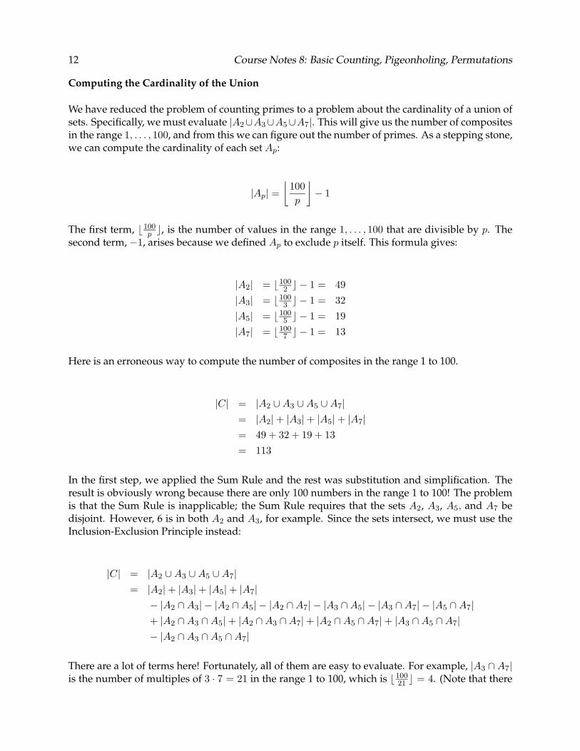
We have reduced the problem of counting primes to a problem about the cardinality of a union of sets. Specifically, we must evaluate |A2 ∪ A3 ∪ A5 ∪ A7|. This will give us the number of composites in the range 1, . . . , 100, and from this we can figure out the number of primes. As a stepping stone, we can compute the cardinality of each set Ap:
|Ap| =
� 100p
− 1
The first term, � 100 �, is the number of values in the range 1, . . . , 100 that are divisible by p. The psecond term, −1, arises because we defined Ap to exclude p itself. This formula gives:
|A2| = � 100 � − 1 = 492
|A3| = � 100 � − 1 = 323
|A5| = � 100 � − 1 = 195
|A7| = � 100 � − 1 = 137
Here is an erroneous way to compute the number of composites in the range 1 to 100.
|C| = |A2 ∪ A3 ∪ A5 ∪ A7| = |A2| + |A3| + |A5| + |A7| = 49 + 32 + 19 + 13
= 113
In the first step, we applied the Sum Rule and the rest was substitution and simplification. The result is obviously wrong because there are only 100 numbers in the range 1 to 100! The problem is that the Sum Rule is inapplicable; the Sum Rule requires that the sets A2, A3, A5, and A7 be disjoint. However, 6 is in both A2 and A3, for example. Since the sets intersect, we must use the Inclusion-Exclusion Principle instead:
|C| = |A2 ∪ A3 ∪ A5 ∪ A7| = |A2| + |A3| + |A5| + |A7|
− |A2 ∩ A3| − |A2 ∩ A5| − |A2 ∩ A7| − |A3 ∩ A5| − |A3 ∩ A7| − |A5 ∩ A7|+ |A2 ∩ A3 ∩ A5| + |A2 ∩ A3 ∩ A7| + |A2 ∩ A5 ∩ A7| + |A3 ∩ A5 ∩ A7|− |A2 ∩ A3 ∩ A5 ∩ A7|
There are a lot of terms here! Fortunately, all of them are easy to evaluate. For example, |A3 ∩ A7|is the number of multiples of 3 · 7 = 21 in the range 1 to 100, which is � 100
21 � = 4. (Note that there
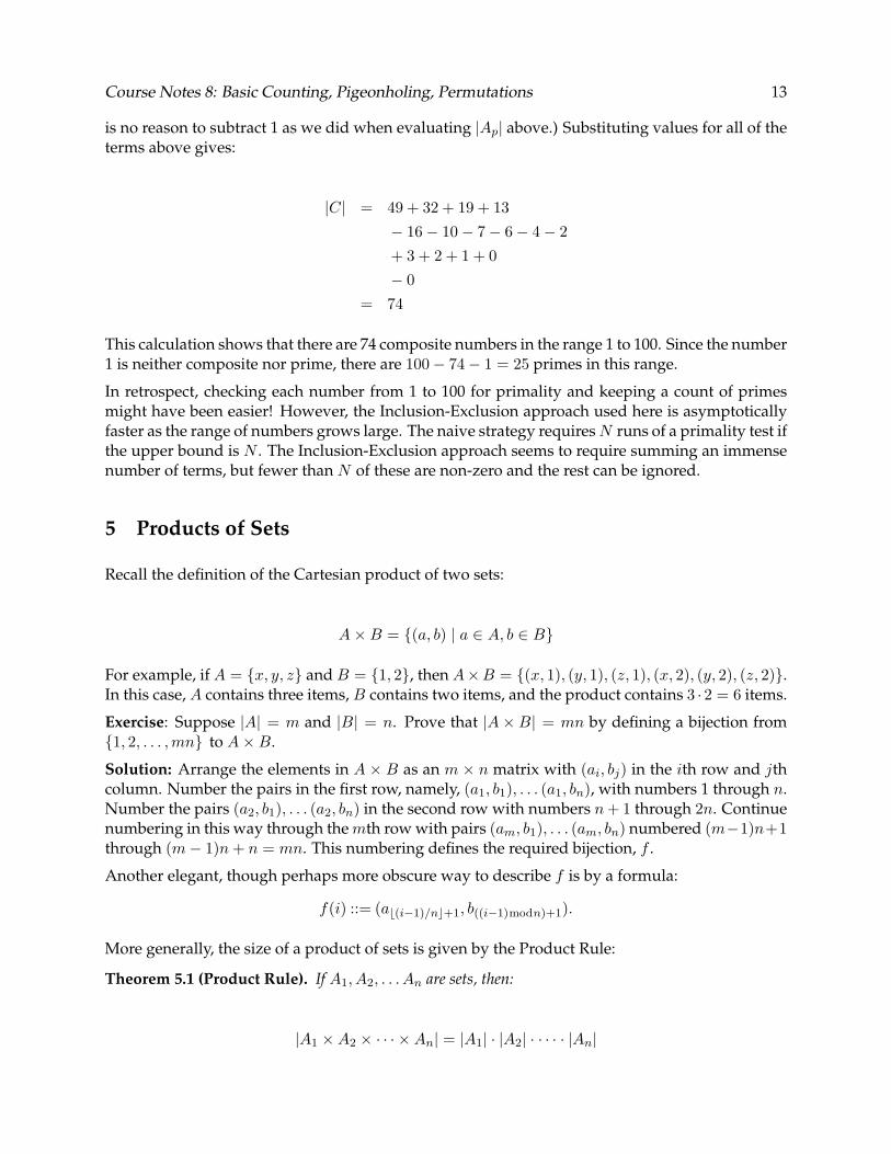
Course Notes 8: Basic Counting, Pigeonholing, Permutations 13
is no reason to subtract 1 as we did when evaluating |Ap| above.) Substituting values for all of the terms above gives:
|C| = 49 + 32 + 19 + 13
− 16 − 10 − 7 − 6 − 4 − 2
+ 3 + 2 + 1 + 0
− 0
= 74
This calculation shows that there are 74 composite numbers in the range 1 to 100. Since the number 1 is neither composite nor prime, there are 100 − 74 − 1 = 25 primes in this range.
In retrospect, checking each number from 1 to 100 for primality and keeping a count of primes might have been easier! However, the Inclusion-Exclusion approach used here is asymptotically faster as the range of numbers grows large. The naive strategy requires N runs of a primality test if the upper bound is N . The Inclusion-Exclusion approach seems to require summing an immense number of terms, but fewer than N of these are non-zero and the rest can be ignored.
5 Products of Sets
Recall the definition of the Cartesian product of two sets:
A × B = {(a, b) | a ∈ A, b ∈ B}
For example, if A = {x, y, z} and B = {1, 2}, then A × B = {(x, 1), (y, 1), (z, 1), (x, 2), (y, 2), (z, 2)}. In this case, A contains three items, B contains two items, and the product contains 3 · 2 = 6 items.
Exercise: Suppose |A| = m and |B| = n. Prove that |A × B| = mn by defining a bijection from {1, 2, . . . ,mn} to A × B.
Solution: Arrange the elements in A × B as an m × n matrix with (ai, bj ) in the ith row and jth column. Number the pairs in the first row, namely, (a1, b1), . . . (a1, bn), with numbers 1 through n. Number the pairs (a2, b1), . . . (a2, bn) in the second row with numbers n + 1 through 2n. Continue numbering in this way through the mth row with pairs (am, b1), . . . (am, bn) numbered (m − 1)n +1 through (m − 1)n + n = mn. This numbering defines the required bijection, f .
Another elegant, though perhaps more obscure way to describe f is by a formula:
f (i) ::= (a�(i−1)/n�+1, b((i−1)modn)+1).
More generally, the size of a product of sets is given by the Product Rule:
Theorem 5.1 (Product Rule). If A1, A2, . . . An are sets, then:
|A1 × A2 × · · · × An| = |A1| · |A2| · · · · · |An|
� �� �
14 Course Notes 8: Basic Counting, Pigeonholing, Permutations
The proof can be done by induction on n, but we leave it to the reader.
Here is another way to look at the product rule: the number of ways to pick one item from A1, 1 item from A2, . . . , and 1 item from An is
� ni=1 |Ai|.
The Product Rule yields a useful generalization of the Pigeonhole Principle:
Theorem 5.2 (Generalized Pigeonhole Principle). If there are m pigeons and n holes, then at least one hole contains �m/n� pigeons.
Proof. Let pi be the number of pigeons in the ith hole, and assume that pi < �m/n� for 1 ≤ i ≤ n. But since pi is an integer, this implies that pi < m/n. By the Product Rule, the total number of pigeons in the holes is p1 · p2 . . . pn < (m/n) · n = m. But all m pigeons are supposed to be in the holes, a contradiction. So some pi must not be less than �m/n�.
Even this Generalized Pigeonhole Priniciple is so obvious that we often take it for granted without explicitly saying so. For example, if you look back in Week 3 Notes at Dilworth’s theorem about the number of chains and antichains in a partial order, you will see we aleady used the Generalized Pigeonhole Principle in proving it.
Four-Course Italian Meals
As an example of the Product Rule, suppose that an Italian restaurant menu lists 15 antipasti, 6 pastas, 10 main courses, and 4 desserts. How many four course-meals are possible? In this case, A1 is the set of antipasti, A2 is the sets of pastas, A3 is the set of main courses, and A4 is the set of desserts. The number of four-course meals is the number of ways of picking one item from each set. By the Product Rule this is:
|A1 × A2 × A3 × A4| = |A1| · |A2| · |A3| · |A4| = 15 · 6 · 10 · 4
= 3600
Now suppose there are 7201 guests at a banquet catered by the restaurant. Then there must be at least three guests who choose exactly the same meal. This follows from the Generalized Pigeon-hole Principle, letting guests be pigeons, four-course meals be holes, and noting that �7201/3600� = 3.
Binary Strings
How many n-bit binary strings are there? If we let B = {0, 1}, then the set of n-bit binary strings is:
B × B × · · · × B
n terms
By the Product Rule, the number of binary strings is |B|n = 2n .

Course Notes 8: Basic Counting, Pigeonholing, Permutations 15
Telephone Numbers
How many telephone numbers are there? There are actually two formats for telephone numbers, an old one and a new one. The formats can be defined in terms of three sets of digits:
A = {0, 1, . . . , 9}
B = {2, 3, . . . , 9}
C = {0, 1}
The old format is (BCA) BBA − AAAA and the new format is (BAA) BAA − AAAA. This gives:
old numbers =
=
=
new numbers =
=
=
|B| · |C| · |A| · |B| · |B| · |A| · |A| · |A| · |A| · |A|2 · 83 · 106
1.024 billion|B| · |A| · |A| · |B| · |A| · |A| · |A| · |A| · |A| · |A|82 · 108
6.4 billion
The reason for the new format is that there are more numbers. In particular, the number of area codes is increased from 8 · 2 · 10 = 160 to 8 · 10 · 10 = 800.
Passwords
Suppose that a password consists of 8 characters where each character is either a number or a lowercase letter. A password is legal if there is at least one number and at least one letter. How many legal passwords are there?
We can solve this problem by “counting the complement”. We used this method earlier to find the number of primes in the range 1 to 100 by counting the composites in this range. In this case, we can find the number of legal passwords by counting the illegal passwords. An illegal password has either all numbers or all letters. By the Product Rule, the number of passwords with all numbers is 108 , and the number of passwords with all letters is 268 . Also by the Product Rule, the total number of passwords (both legal and illegal) is 368 . Therefore, the total number of legal passwords is 368 − 268 − 108 .
6 Tree Diagrams
The Sum and Product Rules are both useful in counting the number of ways that something can be done. In more complicated problems, we need to combine these rules. In such cases, tree diagrams are helpful.
16 Course Notes 8: Basic Counting, Pigeonholing, Permutations
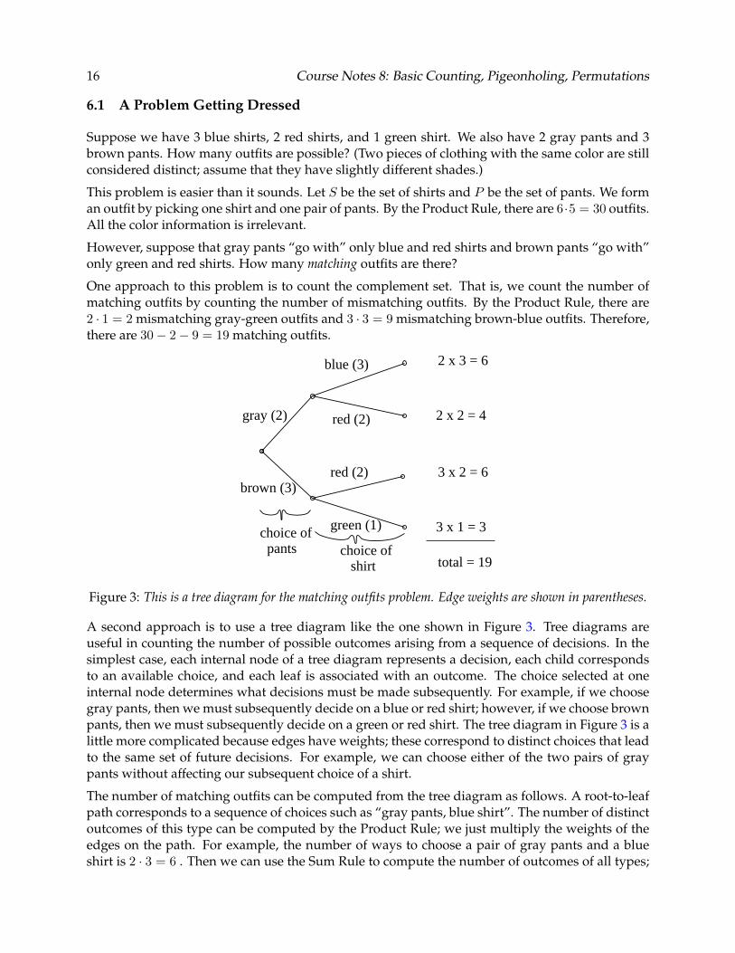
6.1 A Problem Getting Dressed
Suppose we have 3 blue shirts, 2 red shirts, and 1 green shirt. We also have 2 gray pants and 3 brown pants. How many outfits are possible? (Two pieces of clothing with the same color are still considered distinct; assume that they have slightly different shades.)
This problem is easier than it sounds. Let S be the set of shirts and P be the set of pants. We form an outfit by picking one shirt and one pair of pants. By the Product Rule, there are 6 ·5 = 30 outfits. All the color information is irrelevant.
However, suppose that gray pants “go with” only blue and red shirts and brown pants “go with” only green and red shirts. How many matching outfits are there?
One approach to this problem is to count the complement set. That is, we count the number of matching outfits by counting the number of mismatching outfits. By the Product Rule, there are 2 · 1 = 2 mismatching gray-green outfits and 3 · 3 = 9 mismatching brown-blue outfits. Therefore, there are 30 − 2 − 9 = 19 matching outfits.
brown (3)
gray (2)
blue (3)
choice of pants choice of
shirt
2 x 3 = 6
green (1)
red (2) 2 x 2 = 4
3 x 2 = 6
3 x 1 = 3
total = 19
red (2)
Figure 3: This is a tree diagram for the matching outfits problem. Edge weights are shown in parentheses.
A second approach is to use a tree diagram like the one shown in Figure 3. Tree diagrams are useful in counting the number of possible outcomes arising from a sequence of decisions. In the simplest case, each internal node of a tree diagram represents a decision, each child corresponds to an available choice, and each leaf is associated with an outcome. The choice selected at one internal node determines what decisions must be made subsequently. For example, if we choose gray pants, then we must subsequently decide on a blue or red shirt; however, if we choose brown pants, then we must subsequently decide on a green or red shirt. The tree diagram in Figure 3 is a little more complicated because edges have weights; these correspond to distinct choices that lead to the same set of future decisions. For example, we can choose either of the two pairs of gray pants without affecting our subsequent choice of a shirt.
The number of matching outfits can be computed from the tree diagram as follows. A root-to-leaf path corresponds to a sequence of choices such as “gray pants, blue shirt”. The number of distinct outcomes of this type can be computed by the Product Rule; we just multiply the weights of the edges on the path. For example, the number of ways to choose a pair of gray pants and a blue shirt is 2 · 3 = 6 . Then we can use the Sum Rule to compute the number of outcomes of all types;
Course Notes 8: Basic Counting, Pigeonholing, Permutations 17
we just add up all the products. This gives 6 + 4 + 3 + 6 = 19 matching outfits. This is the same number we found by the method of counting the complement. (Good thing!)
Tree diagrams are a more sophisticated example of the case analysis we did for phone numbers. They use cases to break up the top level set, then use more cases to break up each subset, and so on.
6.2 Playoff Outcomes
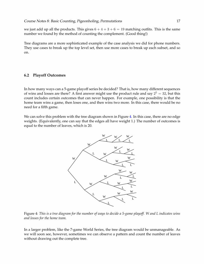
In how many ways can a 5-game playoff series be decided? That is, how many different sequences of wins and losses are there? A first answer might use the product rule and say 25 = 32, but this count includes certain outcomes that can never happen. For example, one possibility is that the home team wins a game, then loses one, and then wins two more. In this case, there would be no need for a fifth game.
We can solve this problem with the tree diagram shown in Figure 4. In this case, there are no edge weights. (Equivalently, one can say that the edges all have weight 1.) The number of outcomes is equal to the number of leaves, which is 20.
W
W
W
LW
LW
L
L W
WL
WL
L WW
L L
LW
W
W
L
WL
L WW
LL
LW
WW
LL L
Figure 4: This is a tree diagram for the number of ways to decide a 5-game playoff. W and L indicates wins and losses for the home team.
In a larger problem, like the 7-game World Series, the tree diagram would be unmanageable. As we will soon see, however, sometimes we can observe a pattern and count the number of leaves without drawing out the complete tree.
18 Course Notes 8: Basic Counting, Pigeonholing, Permutations
7 Permutations
7.1 Simple Permutations
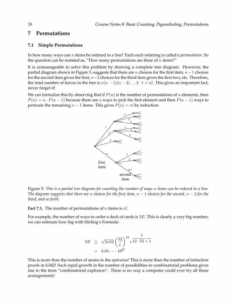
In how many ways can n items be ordered in a line? Each such ordering is called a permutation. So the question can be restated as, “How many permutations are there of n items?”
It is unmanageable to solve this problem by drawing a complete tree diagram. However, the partial diagram shown in Figure 5, suggests that there are n choices for the first item, n − 1 choices for the second item given the first, n−2 choices for the third item given the first two, etc. Therefore, the total number of leaves in the tree is n(n − 1)(n − 2) . . . 2 · 1 = n!. This gives an important fact; never forget it!
We can formalize this by observing that if P (n) is the number of permutations of n elements, then P (n) = n · P (n − 1) because there are n ways to pick the first element and then P (n − 1) ways to permute the remaining n − 1 items. This gives P (n) = n! by induction.
1
2
3
2
3n
13
n
n 1
2
n-1
firstitem
second item
Figure 5: This is a partial tree diagram for counting the number of ways n items can be ordered in a line. The diagram suggests that there are n choices for the first item, n − 1 choices for the second, n − 2 for the third, and so forth.
Fact 7.1. The number of permutations of n items is n!.
For example, the number of ways to order a deck of cards is 52!. This is clearly a very big number; we can estimate how big with Stirling’s Formula:
52! ≥√ �
522π52
e
�52
e
1
12 · 52 + 1
= 8.05 · · · · 1067
This is more than the number of atoms in the universe! This is more than the number of induction proofs in 6.042! Such rapid growth in the number of possibilities in combinatorial problems gives rise to the term “combinatorial explosion”. There is no way a computer could ever try all these arrangements!
Course Notes 8: Basic Counting, Pigeonholing, Permutations 19
7.2 A Lower Bound for Sorting
The fact that there are n! ways to order n items can be combined with the Pigeonhole Principle to prove a nice lower bound on the number of comparisons needed to sort a list of n items.
Theorem 7.2. Any comparison-based sorting algorithm must make at least the following number of comparisons to sort n items in the worst case:
n log2 n − n log2 e
In a comparison-based sorting algorithm, we can compare two items and move items around in memory. All other operations on items, such as looking at certain bits or performing arithmetic on items, are ruled out. For example, there is a sorting algorithm called “bucket sort” that is not comparison-based and for which this theorem does not apply.
The idea behind the proof is the same as in the twenty-questions game in Section 3.3 above. There we compared the number of possible locations of the counterfeit coin with the number of leaves in a decision tree defined by our weighing scheme. Here we compare the number of initial permutations of items with the number of leaves in a computation tree defined by the sorting algorithm.
Proof. Let x1, . . . , xn be the items to be sorted. Since we are proving a lower bound, we can assume that the items are all distinct.
Let A be any sorting algorithm. Algorithm A must permute the items x1, . . . , xn to put them in the correct order. Since a different permutation is required for each different initial ordering of the items, the number of different permutations that might be required is n!.
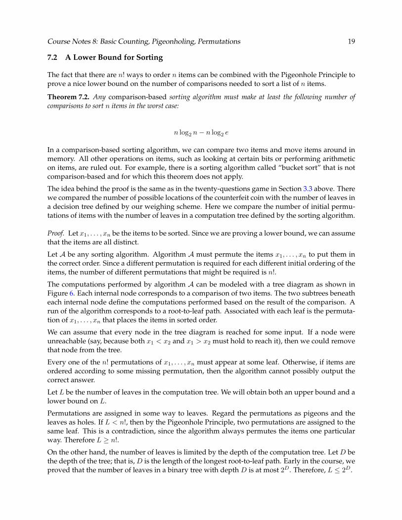
The computations performed by algorithm A can be modeled with a tree diagram as shown in Figure 6. Each internal node corresponds to a comparison of two items. The two subtrees beneath each internal node define the computations performed based on the result of the comparison. A run of the algorithm corresponds to a root-to-leaf path. Associated with each leaf is the permutation of x1, . . . , xn that places the items in sorted order.
We can assume that every node in the tree diagram is reached for some input. If a node were unreachable (say, because both x1 < x2 and x1 > x2 must hold to reach it), then we could remove that node from the tree.
Every one of the n! permutations of x1, . . . , xn must appear at some leaf. Otherwise, if items are ordered according to some missing permutation, then the algorithm cannot possibly output the correct answer.
Let L be the number of leaves in the computation tree. We will obtain both an upper bound and a lower bound on L.
Permutations are assigned in some way to leaves. Regard the permutations as pigeons and the leaves as holes. If L < n!, then by the Pigeonhole Principle, two permutations are assigned to the same leaf. This is a contradiction, since the algorithm always permutes the items one particular way. Therefore L ≥ n!.
On the other hand, the number of leaves is limited by the depth of the computation tree. Let D be the depth of the tree; that is, D is the length of the longest root-to-leaf path. Early in the course, we proved that the number of leaves in a binary tree with depth D is at most 2D . Therefore, L ≤ 2D .
20 Course Notes 8: Basic Counting, Pigeonholing, Permutations
2nd compare
3rdcompare
1st compare><
><
>< >< < > <>
x1 vs x2
x3 vs x4x4 vs x7
x4 vs x7 x2 vs x6x1 vs x5
output
x5 vs x6
x1 x4 x9 x6 ...
Figure 6: This is how the computation tree of a sorting algorithm might look.
Since D is the length of the longest root-to-leaf path in the computation tree, D is the number of comparisons used by algorithm A in the worst case. We can get a lower bound on D by putting together the upper and lower bounds on the number of leaves L.
2D ≥ L ≥ n! D ≥ log2 n!
Now we can use Stirling’s Formula to make sense of log2 n!:
1 √ � n �n
D ≥ log2 2πn e 12n + 1 e
1 log2 e = n log2 n − n log2 e +
2 log2(2πn) +
12n + 1 ≥ n log2 n − n log2 e
How tight is this lower bound? The Merge Sort algorithm is a familiar, comparison-based sorting algorithm covered in most algorithms texts that is known to take at most n log2 n − n + 1 compar-isons.1 Our lower bound implies that at least n log2 n − 1.45n comparisons are necessary in the worst case. The difference between this achievable number of comparisons and out lower bound is only about n/2. So our bound cannot be improved by more than the low-order term n/2. This also follows that Merge Sort cannot be improved by more than this low-order term—Merge Sort is very nearly optimal!
1Rosen, p 569.
Course Notes 8: Basic Counting, Pigeonholing, Permutations 21
8 r-Permutations
In a horse race, the first-place horse is said to “win”, the second-place horse is said to “place”, and the third-place horse is said to “show”. A bet in which one guesses exactly which horses will win, place, and show is called a Trifecta. How many possible Trifecta bets are there in a race with 10 horses? This problem is easy enough that we do not need to draw out the tree diagram; there are 10 choices to win, 9 choices to place given the winner, and 8 choices to show given the first two finishers. This gives 10 · 9 · 8 = 720 possible Trifecta bets.
This is a special case of a standard problem: counting r-permutations of a set.
Definition 8.1. An r-permutation of a set is an ordering of r distinct items from the set.
For example, the 2-permutations of the set {A,B, C} are:
(A,B) (A,C) (B,C) (B,A) (C,A) (C,B)
The number of r-permutations of an n-element set comes up so often in combinatorial problems that there is a special notation.
Definition 8.2. P (n, r) denotes the number of r-permutations of an n-element set. In other words,
n! P (n, r) = n(n − 1) . . . (n − r + 1) =
(n − r)!
For example, the number of Trifecta bets in a 10 horse race is P (10, 3) =10!
= 720.7!
Example 8.3. How many strings of 5 letters are there with no repetitions? For example, ZYGML, issuch a string. In general, these strings are exactly the 5-permutations of the set of letters. Therefore,
there are P (26, 5) =26!21!
, which is 7,893,600.
Example 8.4. How many ways can 5 students be chosen from a class of 180 to be given 5 fabulous (different) prizes, say $1000, $500, $250, $100, $50? Answer: P (180, 5), which is 180 × 179 × 178 × 177 × 176.
Example 8.5. How many injective functions are there from A to B, if |A| = n and |B| = m (assume n ≤ m). Answer: Order A arbitrarily. The first element maps somewhere in B. The second element maps somewhere else (injective), etc. The number of possibilities is P (m,n) = m(m −
1)(m − 2) . . . (m − n + 1) =m!
(m − n)!. Essentially this is picking a sequence of n of the m elements
of B.