Bayesian uncertainty quantification and …Bayesian uncertainty quantification and propagation for the DEM We consider a parametrized class M of a Force–Displacement model, and let

Available online at www.sciencedirect.com

ScienceDirect

Comput. Methods Appl. Mech. Engrg. 282 (2014) 218–238www.elsevier.com/locate/cma

Bayesian uncertainty quantification and propagation for discreteelement simulations of granular materials

P.E. Hadjidoukasa, P. Angelikopoulosa, D. Rossinellia, D. Alexeeva, C. Papadimitrioub,P. Koumoutsakosa,∗

a Computational Science and Engineering Laboratory, ETH Zurich, CH-8092, Switzerlandb Department of Mechanical Engineering, University of Thessaly, Pedion Areos, GR-38334 Volos, Greece

Received 31 January 2014; received in revised form 30 June 2014; accepted 18 July 2014Available online 11 August 2014

Abstract

Predictions in the behavior of granular materials using Discrete Element Methods (DEM) hinge on the employed interaction po-tentials. Here we introduce a data driven, Bayesian framework to quantify DEM predictions. Our approach relies on experimentallymeasured coefficients of restitution for single steel particle–wall collisions. The calibration data entail both tangential and normalcoefficients of restitution, for varying impact angles and speeds of the bouncing particle. The parametric uncertainty in multipleForce–Displacement models is estimated using an enhanced Transitional Markov Chain Monte Carlo implemented efficiently onparallel computer architectures. In turn, the parametric model uncertainties are propagated to predict Quantities of Interest (QoI)for two testbed applications: silo discharge and vibration induced mass-segregation. This work demonstrates that the classical wayof calibrating DEM potentials, through parameter optimization, is insufficient and it fails to provide robust predictions. The presentBayesian framework provides robust predictions for the behavior of granular materials using DEM simulations. Most importantlythe results demonstrate the importance of including parametric and modeling uncertainties in the potentials employed in DiscreteElement Methods.c⃝ 2014 Elsevier B.V. All rights reserved.

Keywords: Uncertainty quantification; Bayesian model selection; Discrete Element Method; Contact force models; Granular flow

1. Introduction

The Discrete Element Method (DEM) [1] is a powerful technique for simulating particle models of engineering sys-tems. It is the main tool of computational investigation in engineering applications [2] including Silo discharge [3–6],wave propagation through granular media [7], particle mixing on grates and in drums [8–10], fluidized beds [11,12]and plug flows [13].

∗ Correspondence to: Computational Science and Engineering Laboratory, ETH Zurich, Clausiusstrasse 33, CH-8092, Switzerland. Tel.: +41 44632 52 58; fax: +41 44 632 17 03.

E-mail address: [email protected] (P. Koumoutsakos).

http://dx.doi.org/10.1016/j.cma.2014.07.0170045-7825/ c⃝ 2014 Elsevier B.V. All rights reserved.

http://crossmark.crossref.org/dialog/?doi=10.1016/j.cma.2014.07.017&domain=pdf

http://www.elsevier.com/locate/cma

http://dx.doi.org/10.1016/j.cma.2014.07.017

http://www.elsevier.com/locate/cma

mailto:[email protected]


P.E. Hadjidoukas et al. / Comput. Methods Appl. Mech. Engrg. 282 (2014) 218–238 219

The core of DEM is the selected Force–Displacement (F–D) model that updates the rotational and translationalmovement for each particle following pairwise collisions with other particles and obstacles. The F–D model reflectsthe nature of the material and is a low order model of the detailed viscoelastic interactions of each particle withits environment. However F–D models are semi-empirical and often contain several parameters to be identified.The sensitivity of various Quantities of Interest (QoIs) in DEM simulations to the F–D model parameters has beenthe subject of several investigations [5,14–17]. The common practice is that DEM parameters are calibrated usingexperimental measurements, without taking into account the experimental and model uncertainty. The search for anoptimal DEM model has led to extensive comparative studies [18,19] of different models and parameters. The studiesreported in [19] demonstrated the difficulty in defining and asserting the superiority of one model over the others.

Here we investigate the parameters and structure of F–D models in DEM using a Bayesian framework [20–26].A probabilistic Bayesian Uncertainty Quantification and Propagation (UQ+P) framework is used to quantify andcalibrate parameter uncertainties in DEM simulations based on available experimental measurements from systemcomponents. Furthermore we propagate these uncertainties in DEM simulations to make robust predictions forrelevant QoI.

We focus on evaluating the quantitative predictions of three different F–D models using experimental data fornormal and tangential restitution coefficients. The uncertainty in the parameters of these models is estimated, and themost probable model is identified. In turn we propagate uncertainties to QoI in simulations of applications such asSilo Discharge blocking and the “Brazil Nut” effect [27]. We employ an enhanced parallel variant of the TransitionalMarkov Chain Monte Carlo (TMCMC) algorithm [28,29] along with a parallel framework to distribute the largenumber of system runs in clusters with heterogeneous computer architectures [30]. Our results help demonstrate thevalue of the Bayesian framework for DEM simulations and provide credible intervals for their predictions.

The paper is organized as follows: In Section 2 we outline the elements of DEM simulations and in particularthe parametric F–D models. Section 3 presents the Bayesian framework and in Section 4 we give the results for theBayesian Calibration of the F–D model parameters. Section 5 showcases two UQ+P studies on relevant industrialapplications using the calibrated uncertainty models from Section 4. Our summary and conclusions are presented inSection 6.

2. The DEM and its implementation

The DEM is a widely used method to simulate granular material with a broad range of industrial applicationsranging from oil and gas to pharmaceutical and metallurgy. The granular material is modeled as a set of particles ofvarious shapes with translational and rotational degrees of freedom accompanied by models of interparticle collisions.Each particle has its own mass, velocity and contact properties. The contact forces between particles consist of elastic,viscous and frictional resistance forces.

In this work we consider two-dimensional systems. Two disks with radii Ri , R j are assumed to be in mechanicalcontact if ξi j ≡ Ri + R j −

ri − r j > 0. Here ri − r j = ri j is the vector connecting the center of particle i to

the center of particle j and ξi j is the mutual compression between the particles (see Fig. 1). The force exerted onparticle i due to contact with particle j is given as Fi j = Fn

i j + Fti j where

F t

and (Fn) are its tangential and normal

contributions (see 1). Following the notation of [31] the normal and the tangential contact force components can bewritten as

Fni j = Fn

i j eni j , Ft

i j = F ti j e

ti j (1)

with the unit vectors

eni j =

rj − rirj − ri , et

i j =

0 −11 0

· en

i j .

Particles evolve according to the two-dimensional Newton’s equations of motion (2):

mi ri = mi g +

Nj, j=i

Fi j , Ii φi =

Nj, j=i

li j × Fi j

· ez

i j

ri = ri0, ri = 0, φi = 0, φi = 0 (2)

220 P.E. Hadjidoukas et al. / Comput. Methods Appl. Mech. Engrg. 282 (2014) 218–238

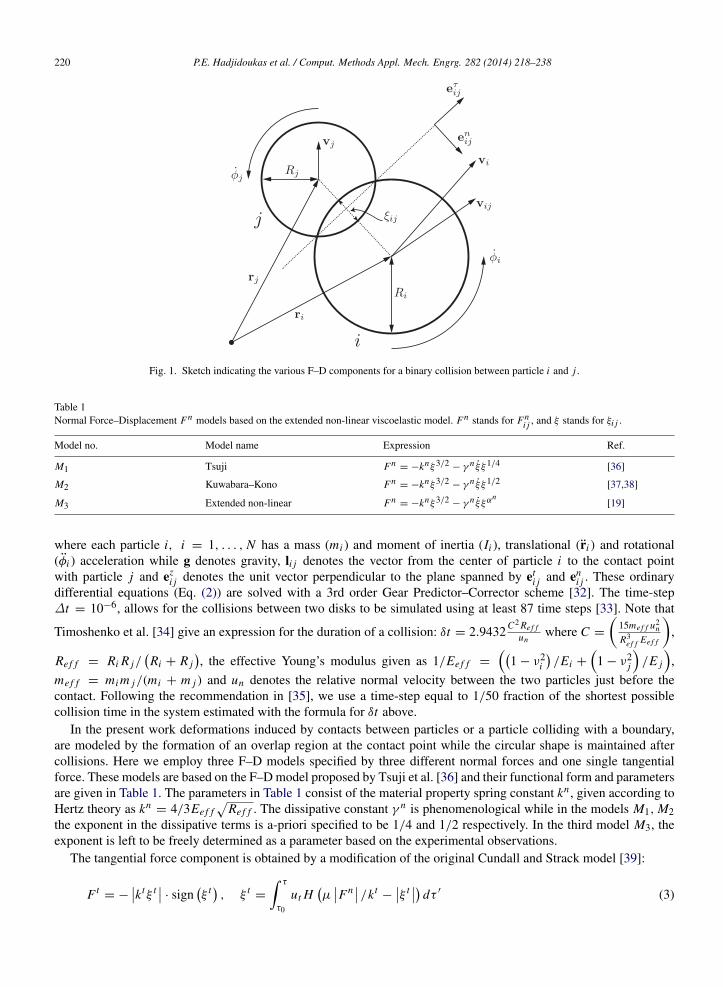
Fig. 1. Sketch indicating the various F–D components for a binary collision between particle i and j .

Table 1Normal Force–Displacement Fn models based on the extended non-linear viscoelastic model. Fn stands for Fn

i j , and ξ stands for ξi j .

Model no. Model name Expression Ref.

M1 Tsuji Fn= −knξ3/2

− γ n ξ ξ1/4 [36]

M2 Kuwabara–Kono Fn= −knξ3/2

− γ n ξ ξ1/2 [37,38]

M3 Extended non-linear Fn= −knξ3/2

− γ n ξ ξαn[19]

where each particle i, i = 1, . . . , N has a mass (mi ) and moment of inertia (Ii ), translational (ri ) and rotational(φi ) acceleration while g denotes gravity, li j denotes the vector from the center of particle i to the contact pointwith particle j and ez

i j denotes the unit vector perpendicular to the plane spanned by eti j and en

i j . These ordinarydifferential equations (Eq. (2)) are solved with a 3rd order Gear Predictor–Corrector scheme [32]. The time-step∆t = 10−6, allows for the collisions between two disks to be simulated using at least 87 time steps [33]. Note that

Timoshenko et al. [34] give an expression for the duration of a collision: δt = 2.9432 C2 Re f fun

where C =

15me f f u2

n

R3e f f Ee f f

,

Re f f = Ri R j/Ri + R j

, the effective Young’s modulus given as 1/Ee f f =

1 − ν2

i

/Ei +

1 − ν2

j

/E j

,

me f f = mi m j/(mi + m j ) and un denotes the relative normal velocity between the two particles just before thecontact. Following the recommendation in [35], we use a time-step equal to 1/50 fraction of the shortest possiblecollision time in the system estimated with the formula for δt above.

In the present work deformations induced by contacts between particles or a particle colliding with a boundary,are modeled by the formation of an overlap region at the contact point while the circular shape is maintained aftercollisions. Here we employ three F–D models specified by three different normal forces and one single tangentialforce. These models are based on the F–D model proposed by Tsuji et al. [36] and their functional form and parametersare given in Table 1. The parameters in Table 1 consist of the material property spring constant kn , given according toHertz theory as kn

= 4/3Ee f f

Re f f . The dissipative constant γ n is phenomenological while in the models M1, M2the exponent in the dissipative terms is a-priori specified to be 1/4 and 1/2 respectively. In the third model M3, theexponent is left to be freely determined as a parameter based on the experimental observations.

The tangential force component is obtained by a modification of the original Cundall and Strack model [39]:

F t= −

ktξ t · sign

ξ t , ξ t

=

τ

τ0

ut Hµ

Fn /kt

−ξ t

dτ ′ (3)


where H is the Heaviside function, kt and µ are phenomenological parameters modeling the tangential spring stiffnessand friction, τ0 is the time when the collision between disk i and j starts, τ > τ0 is the time when we evaluate the forceand ut denotes the relative tangential velocity between the two particles at their contact point. Collisions of particleswith rigid walls are represented by collisions with phantom disks with a very small curvature [40]. This method treatsthe walls as a smooth boundary surface allowing for inelastic collisions.

3. Bayesian uncertainty quantification and propagation for the DEM

We consider a parametrized class M of a Force–Displacement model, and let θ ∈ RNθ be a set of F–D parameters(e.g. tangential spring stiffness, friction coefficient, dissipative constant) belonging to this model class, that will beestimated using experimental data. The model parameters θ are considered to be uncertain and probability distributionfunctions (PDF) are introduced to quantify their plausible values. A PDF π (θ |M) is assigned to the model parametersincorporating prior information based on previous knowledge or physical limitations.

3.1. Model parameter estimation

In Bayesian inference, the probability distribution of the model parameters θ is updated based on measurementsavailable at a particle–particle, particle–wall or system level. Let D ≡ y = {yr , r = 1, . . . , ny} ∈ Rny be a setof observations (data) available from experiments. The prediction error e ∈ Rn y is introduced to characterize thediscrepancy between the model predictions g (θ |M) ∈ Rny and the corresponding data y. The observation data andthe model predictions satisfy the prediction error equation

y = g (θ |M) + e. (4)

The prediction error is composed of two parts

e = ed+ em, (5)

accounting for the measurement (ed ) and modeling (em) uncertainties, respectively.Experimental data usually are provided in terms of the mean and the variance of each measured quantity so the

maximum entropy principle [41], can be invoked to select a normal distribution for the measurement error term ed .Similarly, this Gaussian assumption is also well justified for the modeling error term em due to the lack of informationfor assigning an alternative distribution.

Assuming zero mean for each error term, we set ed∼ N

0,Σ d

and em

∼ N (0,Σm), where Σ d , and Σm aretaken to be diagonal, due to the fact that measurements and model predictions under different system conditions areindependent. The covariance matrix Σ d

= diagν2

r

, where ν2

r is the variance of the r th observation. The covariancematrix Σm

= diagσ 2

r y2r

of the model error term involves the unknown normalized variance parameters σ 2

r whichare usually included in the uncertain parameter set θ to be determined from the data. It represents the inability of themodel to capture all of the experimental values at all possible scenarios. Letting σ 2

r = σ 2 one obtains the covariancematrix Σm

= σ 2diag(y2r ) involving a single parameter σ 2, scaling the variances of each prediction error quantity

involved in em by its experimental value y2r . Note that Bayesian results depend on the choices of the distributions and

the correlation structure of the modeling errors. However a detailed study of different assumptions on the distributionof the modeling terms is beyond the scope of the current study. The reader is referred to Ref. [42] for the effect ofcorrelation structure of the covariance matrix on the Bayesian results.

The updated distribution f (θ |D, M) of the model parameters θ , given the data D, the model class M and priorinformation about the parameters π (θ |M), is given from the Bayes theorem as

f (θ |D, M) =f (D|θ, M) π (θ |M)

f (D|M)(6)

where f (D|θ, M) is the likelihood of observing the data D from a model corresponding to a value θ of the modelclass M and f (D|M) is the evidence of the model class M , selected such that the posterior distribution f (θ |D, M)

of the model parameters integrates to one.


Using the prediction error equation (4) and assuming that the error terms in (5) are independent, the likelihoodf (D|θ, M) of observing the data follows the multi-variable normal distribution:

f (D|θ, M) =

Σ−1/2

(2π)N/2 exp

−

12

Jθ; y

(7)

where

Jθ; y

=

y − g (θ |M)

T Σ−1 y − g (θ |M)

(8)

is the weighted measure of fit between the F–D model predictions and the measured data, Σ = Σ d+Σm

= diag[ν2r +

σ 2r y2

r ] is the covariance of the prediction error, and |.| denotes a determinant.Stochastic simulation algorithms are used to generate samples from the posterior PDF. Here we use the TMCMC

algorithm [28], a generalization of the methods proposed in [23,43]. To handle the large computational cost associatedwith the TMCMC algorithm, we exploit the parallel nature of the algorithm [29] using a task-stealing library [30].

3.2. Force–displacement model selection

Following the Bayesian calibration of the F–D model, selection between two alternative model classes Mi and M j ,based on the observed data D, can be guided using the Bayes factor [22]

Ki j =f (D|Mi )

f (D|M j ). (9)

A number of µ competing model classes M1, . . . , Mµ are ranked based on their probability given the data D accordingto the Bayes model selection equation

Pr(Mi |D) =f (D|Mi )Pr(Mi )

f (D|M1, . . . , Mµ)(10)

where Pr(Mi ) is the prior probability of the model class Mi . The most probable model class is selected as the one thatmaximizes Pr(Mi |D) over i . The evidence of each model class is evaluated as a by-product of the TMCMC algorithm.

3.3. Uncertainty propagation for robust posterior predictions

Robust posterior predictions of an output QoI Q are obtained by taking into account the updated (posterior) uncer-tainties in the model parameters given the measured data D [44]. Within this work, the robust posterior predictionsare conditioned to the data driven Bayesian identification of the uncertainties in the models and their parameters [25].Let FQ(q|θ, M) be the conditional cumulative distribution of Q given the model parameters θ and the model classM . For Gaussian modeling and measurement errors, the form of the cumulative distribution is simple and does notrequire expensive system simulations. For systems that include uncertain initial condition input excitation uncertain-ties or other stochastic descriptors of its components, the estimation of the conditional cumulative distribution may becomputationally very expensive.

The posterior robust cumulative distribution FQ(q|D, M) of the output quantity Q, taking into account the modelM and the data D, is given by

FQ(q|D, M) = Pr(Q ≥ q|D, M) =

θ

FQ(q|θ, M) f (θ |D, M)dθ. (11)

The robust estimate FQ(q|D, M) represents an average of the conditional cumulative distribution weighted by theposterior probability distribution f (θ |D, M) of the model parameters [45]. The posterior cumulative distributionFQ(q|D, M) quantifies the uncertainty in the QoI Q given the model and the data. Using the samples θ (i), i = 1,

. . . , N drawn from the posterior probability distribution f (θ |D, M), the integral (11) is approximated by the sampleestimate

FQ(q|D, M) ≈1N

Ni=1

FQ(q|θ (i), M). (12)


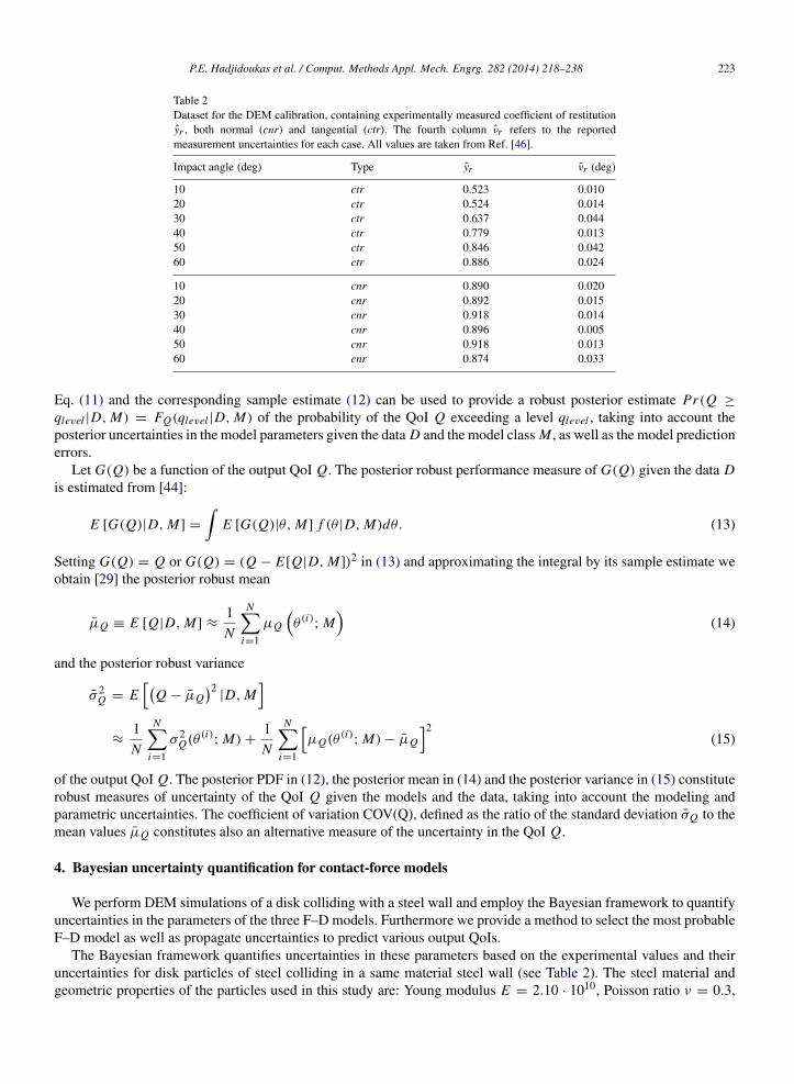
Table 2Dataset for the DEM calibration, containing experimentally measured coefficient of restitutionyr , both normal (cnr) and tangential (ctr). The fourth column νr refers to the reportedmeasurement uncertainties for each case. All values are taken from Ref. [46].

Impact angle (deg) Type yr νr (deg)

10 ctr 0.523 0.01020 ctr 0.524 0.01430 ctr 0.637 0.04440 ctr 0.779 0.01350 ctr 0.846 0.04260 ctr 0.886 0.024

10 cnr 0.890 0.02020 cnr 0.892 0.01530 cnr 0.918 0.01440 cnr 0.896 0.00550 cnr 0.918 0.01360 cnr 0.874 0.033

Eq. (11) and the corresponding sample estimate (12) can be used to provide a robust posterior estimate Pr(Q ≥

qlevel |D, M) = FQ(qlevel |D, M) of the probability of the QoI Q exceeding a level qlevel , taking into account theposterior uncertainties in the model parameters given the data D and the model class M , as well as the model predictionerrors.

Let G(Q) be a function of the output QoI Q. The posterior robust performance measure of G(Q) given the data Dis estimated from [44]:

E [G(Q)|D, M] =

E [G(Q)|θ, M] f (θ |D, M)dθ. (13)

Setting G(Q) = Q or G(Q) = (Q − E[Q|D, M])2 in (13) and approximating the integral by its sample estimate weobtain [29] the posterior robust mean

µQ ≡ E [Q|D, M] ≈1N

Ni=1

µQ

θ (i)

; M

(14)

and the posterior robust variance

σ 2Q = E

Q − µQ

2|D, M

≈

1N

Ni=1

σ 2Q(θ (i)

; M) +1N

Ni=1

µQ(θ (i)

; M) − µQ

2(15)

of the output QoI Q. The posterior PDF in (12), the posterior mean in (14) and the posterior variance in (15) constituterobust measures of uncertainty of the QoI Q given the models and the data, taking into account the modeling andparametric uncertainties. The coefficient of variation COV(Q), defined as the ratio of the standard deviation σQ to themean values µQ constitutes also an alternative measure of the uncertainty in the QoI Q.

4. Bayesian uncertainty quantification for contact-force models

We perform DEM simulations of a disk colliding with a steel wall and employ the Bayesian framework to quantifyuncertainties in the parameters of the three F–D models. Furthermore we provide a method to select the most probableF–D model as well as propagate uncertainties to predict various output QoIs.

The Bayesian framework quantifies uncertainties in these parameters based on the experimental values and theiruncertainties for disk particles of steel colliding in a same material steel wall (see Table 2). The steel material andgeometric properties of the particles used in this study are: Young modulus E = 2.10 · 1010, Poisson ratio ν = 0.3,


Table 3Range of uniform prior PDFs π(θ) of the model parameters for all three model classes.

Class Support of prior PDF π (θ)

M1 [0.05, 0.2] × [0.1, 15.0] × [0.1 · 104, 15.0 · 104] × [0, 1 · 10−2

] × [0, 1 · 10−2]

M2 [0.05, 0.2] × [0.1, 15.0] × [0.1 · 104, 15.0 · 104] × [0, 1 · 10−2

] × [0, 1 · 10−2]

M3 [0.05, 0.2] × [0.15, 1.35] × [0.1, 15.0] × [0.1 · 104, 15.0 · 104] × [0, 1 · 10−2

] × [0, 1 · 10−2]

Table 4Mean values and coefficients of variation (COV) of the posterior distribution of the model parameter, along with the LogEvidencevalues of each model class.

Class µ uµ αn uαn γ n uγ n kt ukt σ1 σ2 LogEvidence

M1 0.109 12.8% 0.25 – 0.81 · 104 17.2% 0.99 35.1% 0.0045 0.0016 15.46M2 0.108 11.77% 0.5 – 8.41 · 104 18.7% 1.01 33.8% 0.0035 0.0019 16.39M3 0.111 9.5% 0.44 5.78% 5.45 · 104 55.5% 1.04 27.9% 0.0045 0.0007 22.41

disk radius Ri = 0.02225 m with a mass of 0.3538 kg. Note that these are the values reported in the experimentalstudy, but are not necessarily exact. One could consider them uncertain, and identify them along with the other modelparameters.

The mean values and the experimental uncertainty in the restitution coefficient measurements are reported inTable 2 for various values of the impact angle between steel particles and a steel wall. We use as data the coefficientsof tangential (ctr) and normal (cnr) restitution for six values of the impact angle ranging from 10 to 60 degrees.The coefficient of normal restitution is the ratio of the post-collisional and the pre-collisional values of the normalcomponent of the relative velocity of the object [47]. Similarly the coefficient of tangential restitution is the ratio ofthe tangential velocity components.

The covariance Σm= diag

Σm

cnr ,Σmctr

of the prediction error model is chosen as a 2 × 2 block diagonal matrix

with each block associated with the ctr and cnr measurements. The diagonal block elements Σmcnr and Σm

ctr are alsoassumed to be diagonal matrices, i.e. Σm

cnr = σ 21 diag

y2

cnr

and Σm

ctr = σ 22 diag

y2

ctr

, dividing in this way the

data into two disjoint groups associated with the normal and tangential coefficient of restitution, respectively. Eachgroup of data involves six measurements and the prediction errors for each one of the measurements are assumedto be independent. Note that the parameter kn was kept fixed to its theoretical value determined using the Youngmodulus, the Poisson ratio and the radius of the considered disks. Although one could have included the parameter kn

in the uncertain vector θ , herein it was decided to keep it fixed to its theoretical value, thus avoiding possible stronginteractions between this parameter and the rest of the F–D model parameters that could result in unrealistic kn valuesfurther away from the theoretical one.

For the model classes M1 and M2 the parameter vector is θ =µ, γ n, kt , σ1, σ2,

involving 3 F–D model param-

eters, and two prediction error parameters. The θ for the third model class is θ =µ, αn, γ n, kt , σ1, σ2,

, including

the exponent αn as an extra parameter. Uniform prior distributions for all parameters are used and their ranges areshown in Table 3.

A parallel TMCMC algorithm [29] is used to generate samples from the posterior PDF of the model parameters. Asensitivity study for the selection of the number of samples per TMCMC stage was performed, indicating that 8192samples were adequate for all model classes considered, since an increase of almost 2 order of magnitude in samplesyielded results that differ insignificantly. The posterior distribution of the model parameters were thus represented bythe 8192 samples obtained at the last TMCMC stage.

The marginal distributions of the parameters for the three model classes M1, M2 and M3 (see Figs. 2–4) are ob-tained using Kernel estimation. The TMCMC samples drawn from the posterior distribution provide sample estimatesof the mean and the standard deviation of the model parameters using Eqs. (14) and (15), respectively. The posteriormean θ and the coefficient of variation (COV) uθ of the model parameters are reported in Table 4 for each modelclass. The COV measures the extent of uncertainty which is defined as the ratio of the sample standard deviation overthe sample mean.


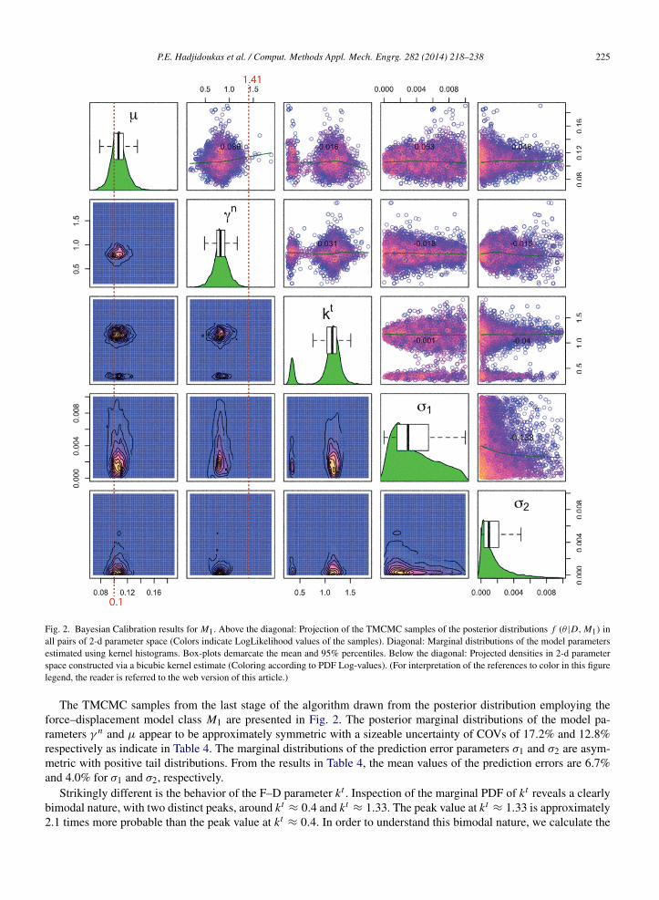
Fig. 2. Bayesian Calibration results for M1. Above the diagonal: Projection of the TMCMC samples of the posterior distributions f (θ |D, M1) inall pairs of 2-d parameter space (Colors indicate LogLikelihood values of the samples). Diagonal: Marginal distributions of the model parametersestimated using kernel histograms. Box-plots demarcate the mean and 95% percentiles. Below the diagonal: Projected densities in 2-d parameterspace constructed via a bicubic kernel estimate (Coloring according to PDF Log-values). (For interpretation of the references to color in this figurelegend, the reader is referred to the web version of this article.)

The TMCMC samples from the last stage of the algorithm drawn from the posterior distribution employing theforce–displacement model class M1 are presented in Fig. 2. The posterior marginal distributions of the model pa-rameters γ n and µ appear to be approximately symmetric with a sizeable uncertainty of COVs of 17.2% and 12.8%respectively as indicate in Table 4. The marginal distributions of the prediction error parameters σ1 and σ2 are asym-metric with positive tail distributions. From the results in Table 4, the mean values of the prediction errors are 6.7%and 4.0% for σ1 and σ2, respectively.

Strikingly different is the behavior of the F–D parameter kt . Inspection of the marginal PDF of kt reveals a clearlybimodal nature, with two distinct peaks, around kt

≈ 0.4 and kt≈ 1.33. The peak value at kt

≈ 1.33 is approximately2.1 times more probable than the peak value at kt

≈ 0.4. In order to understand this bimodal nature, we calculate the


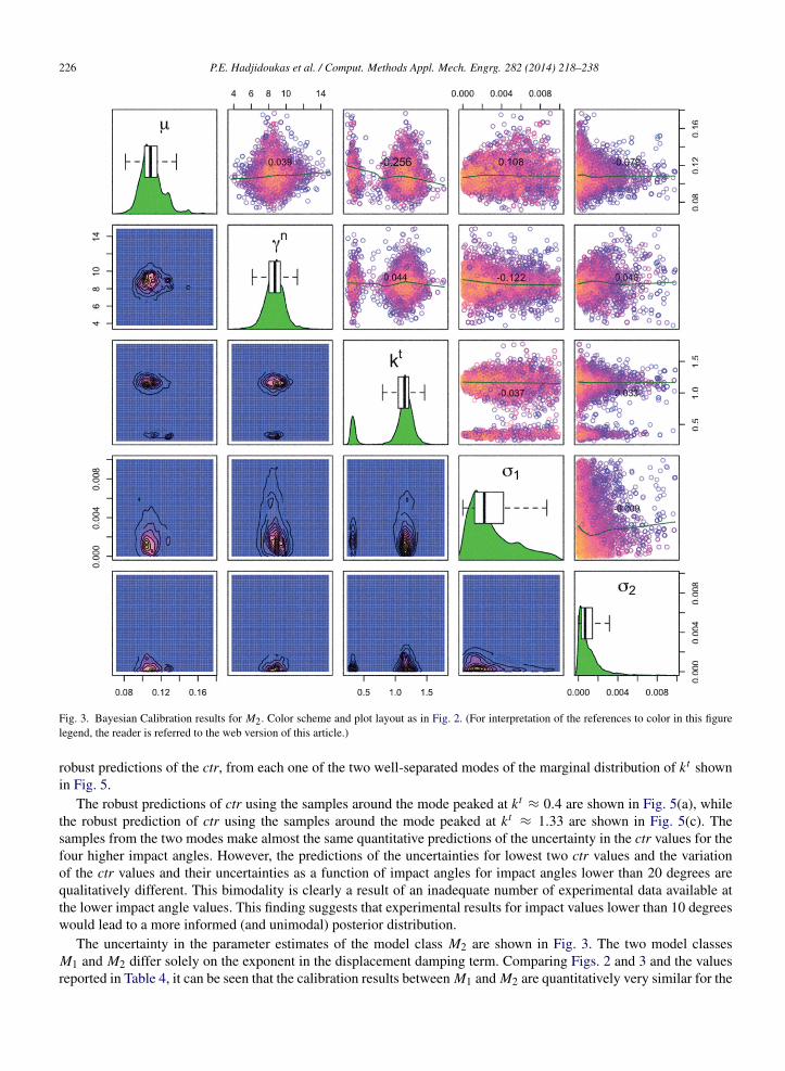
Fig. 3. Bayesian Calibration results for M2. Color scheme and plot layout as in Fig. 2. (For interpretation of the references to color in this figurelegend, the reader is referred to the web version of this article.)

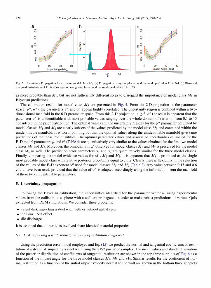
robust predictions of the ctr, from each one of the two well-separated modes of the marginal distribution of kt shownin Fig. 5.

The robust predictions of ctr using the samples around the mode peaked at kt≈ 0.4 are shown in Fig. 5(a), while

the robust prediction of ctr using the samples around the mode peaked at kt≈ 1.33 are shown in Fig. 5(c). The

samples from the two modes make almost the same quantitative predictions of the uncertainty in the ctr values for thefour higher impact angles. However, the predictions of the uncertainties for lowest two ctr values and the variationof the ctr values and their uncertainties as a function of impact angles for impact angles lower than 20 degrees arequalitatively different. This bimodality is clearly a result of an inadequate number of experimental data available atthe lower impact angle values. This finding suggests that experimental results for impact values lower than 10 degreeswould lead to a more informed (and unimodal) posterior distribution.

The uncertainty in the parameter estimates of the model class M2 are shown in Fig. 3. The two model classesM1 and M2 differ solely on the exponent in the displacement damping term. Comparing Figs. 2 and 3 and the valuesreported in Table 4, it can be seen that the calibration results between M1 and M2 are quantitatively very similar for the


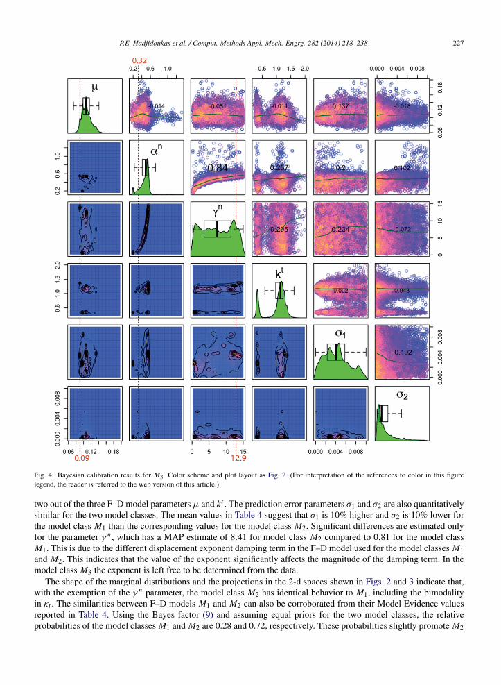
Fig. 4. Bayesian calibration results for M3. Color scheme and plot layout as Fig. 2. (For interpretation of the references to color in this figurelegend, the reader is referred to the web version of this article.)

two out of the three F–D model parameters µ and kt . The prediction error parameters σ1 and σ2 are also quantitativelysimilar for the two model classes. The mean values in Table 4 suggest that σ1 is 10% higher and σ2 is 10% lower forthe model class M1 than the corresponding values for the model class M2. Significant differences are estimated onlyfor the parameter γ n , which has a MAP estimate of 8.41 for model class M2 compared to 0.81 for the model classM1. This is due to the different displacement exponent damping term in the F–D model used for the model classes M1and M2. This indicates that the value of the exponent significantly affects the magnitude of the damping term. In themodel class M3 the exponent is left free to be determined from the data.

The shape of the marginal distributions and the projections in the 2-d spaces shown in Figs. 2 and 3 indicate that,with the exemption of the γ n parameter, the model class M2 has identical behavior to M1, including the bimodalityin κt . The similarities between F–D models M1 and M2 can also be corroborated from their Model Evidence valuesreported in Table 4. Using the Bayes factor (9) and assuming equal priors for the two model classes, the relativeprobabilities of the model classes M1 and M2 are 0.28 and 0.72, respectively. These probabilities slightly promote M2


Fig. 5. Uncertainty Propagation for ctr using model class M1. (a) Propagation using samples around the mode peaked at kt≈ 0.4. (b) Bi-modal

marginal distribution of kt . (c) Propagation using samples around the mode peaked at kt≈ 1.33.

as more probable than M1, but are not sufficiently different so as to disregard the importance of model class M1 inBayesian predictions.

The calibration results for model class M3 are presented in Fig. 4. From the 2-D projection in the parameterspace (γ n , αn), the parameters γ n and αn appear highly correlated. The uncertainty region is confined within a two-dimensional manifold in the 6-D parameter space. From this 2-D projection in (γ n , αn) space it is apparent that theparameter γ n is unidentifiable with most probable values ranging over the whole domain of variation from 0.1 to 15considered in the prior distribution. The optimal values and the uncertainty regions for the γ n parameter predicted bymodel classes M1 and M2 are clearly subsets of the values predicted by the model class M3 and contained within theunidentifiable manifold. It is worth pointing out that the optimal values along the unidentifiable manifold give samepredictions of the measured quantities. The optimal parameter values and associated uncertainties estimated for theF–D model parameters µ and kt (Table 4) are quantitatively very similar to the values obtained for the first two modelclasses M1 and M2. Moreover, the bimodality in kt observed for model classes M1 and M2 is preserved for the modelclass M3 as well. The prediction error parameters σ1 and σ2 are quantitatively similar for the three model classes.Finally, comparing the model evidence values for M1, M2 and M3, it is apparent that M3 is promoted as the singlemost probable model class with relative posterior probability equal to unity. Clearly there is flexibility in the selectionof the values of the F–D exponent αn used for model classes M1 and M2 (Table 2). Any value between 0.15 and 0.6could have been used, provided that the value of γ n is adapted accordingly using the information from the manifoldof these two unidentifiable parameters.

5. Uncertainty propagation

Following the Bayesian calibration, the uncertainties identified for the parameter vector θ , using experimentalvalues from the collision of a sphere with a wall are propagated in order to make robust predictions of various QoIsextracted from DEM simulations. We consider three problems:

• a steel disk impacting a steel wall, with or without initial spin.• the Brazil Nut effect• silo discharge

It is assumed that all particles involved share identical material properties.

5.1. Disk impacting a wall: robust prediction of restitution coefficient

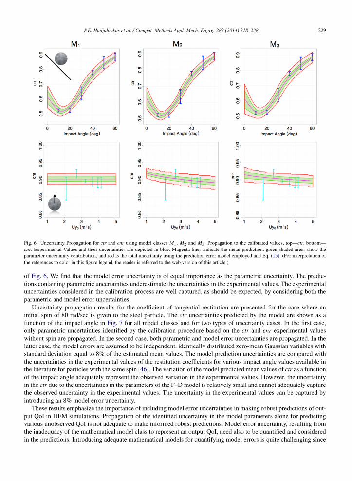
Using the prediction error model employed and Eq. (15) we predict the normal and tangential coefficients of resti-tution of a steel disk impacting a steel wall using the 8192 posterior samples. The mean values and standard deviationof the posterior distribution of coefficients of tangential restitution are shown in the top three subplots of Fig. 6 as afunction of the impact angle for the three model classes M1, M2 and M3. Similar results for the coefficient of nor-mal restitution as a function of the initial impact velocity normal to the wall are shown in the bottom three subplots


Fig. 6. Uncertainty Propagation for ctr and cnr using model classes M1, M2 and M3. Propagation to the calibrated values, top—ctr, bottom—cnr. Experimental Values and their uncertainties are depicted in blue. Magenta lines indicate the mean prediction, green shaded areas show theparameter uncertainty contribution, and red is the total uncertainty using the prediction error model employed and Eq. (15). (For interpretation ofthe references to color in this figure legend, the reader is referred to the web version of this article.)

of Fig. 6. We find that the model error uncertainty is of equal importance as the parametric uncertainty. The predic-tions containing parametric uncertainties underestimate the uncertainties in the experimental values. The experimentaluncertainties considered in the calibration process are well captured, as should be expected, by considering both theparametric and model error uncertainties.

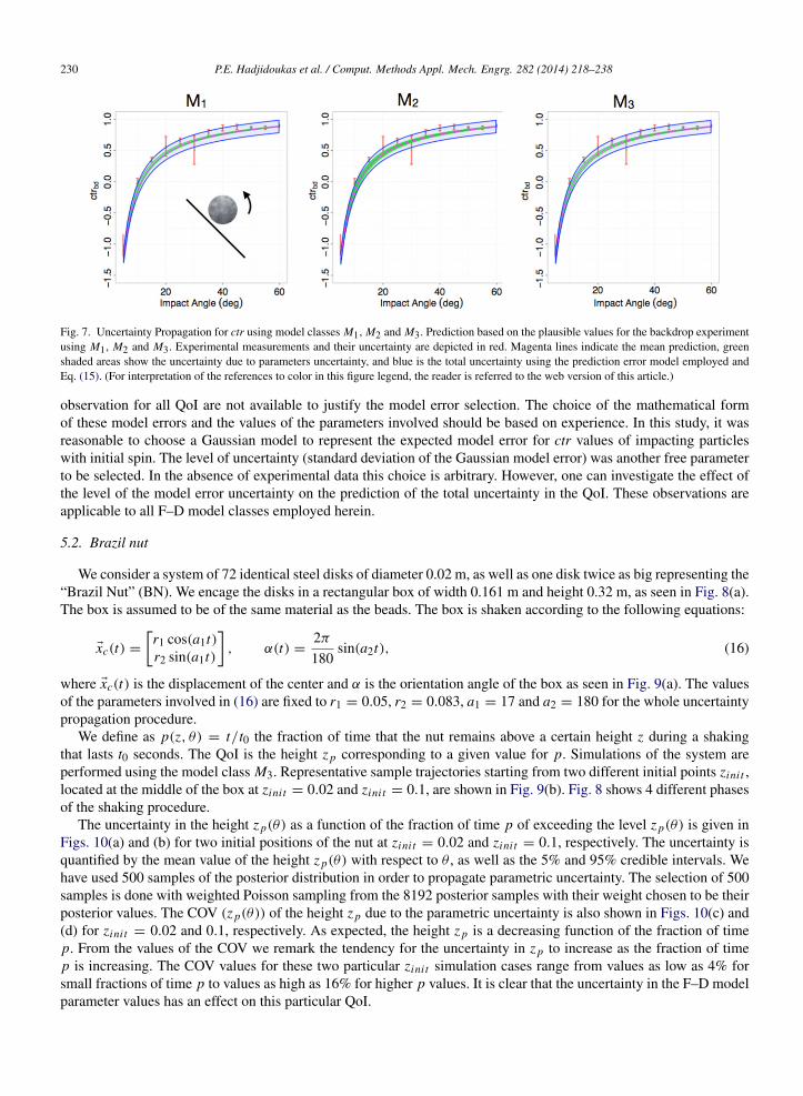
Uncertainty propagation results for the coefficient of tangential restitution are presented for the case where aninitial spin of 80 rad/sec is given to the steel particle. The ctr uncertainties predicted by the model are shown as afunction of the impact angle in Fig. 7 for all model classes and for two types of uncertainty cases. In the first case,only parametric uncertainties identified by the calibration procedure based on the ctr and cnr experimental valueswithout spin are propagated. In the second case, both parametric and model error uncertainties are propagated. In thelatter case, the model errors are assumed to be independent, identically distributed zero-mean Gaussian variables withstandard deviation equal to 8% of the estimated mean values. The model prediction uncertainties are compared withthe uncertainties in the experimental values of the restitution coefficients for various impact angle values available inthe literature for particles with the same spin [46]. The variation of the model predicted mean values of ctr as a functionof the impact angle adequately represent the observed variation in the experimental values. However, the uncertaintyin the ctr due to the uncertainties in the parameters of the F–D model is relatively small and cannot adequately capturethe observed uncertainty in the experimental values. The uncertainty in the experimental values can be captured byintroducing an 8% model error uncertainty.

These results emphasize the importance of including model error uncertainties in making robust predictions of out-put QoI in DEM simulations. Propagation of the identified uncertainty in the model parameters alone for predictingvarious unobserved QoI is not adequate to make informed robust predictions. Model error uncertainty, resulting fromthe inadequacy of the mathematical model class to represent an output QoI, need also to be quantified and consideredin the predictions. Introducing adequate mathematical models for quantifying model errors is quite challenging since


Fig. 7. Uncertainty Propagation for ctr using model classes M1, M2 and M3. Prediction based on the plausible values for the backdrop experimentusing M1, M2 and M3. Experimental measurements and their uncertainty are depicted in red. Magenta lines indicate the mean prediction, greenshaded areas show the uncertainty due to parameters uncertainty, and blue is the total uncertainty using the prediction error model employed andEq. (15). (For interpretation of the references to color in this figure legend, the reader is referred to the web version of this article.)

observation for all QoI are not available to justify the model error selection. The choice of the mathematical formof these model errors and the values of the parameters involved should be based on experience. In this study, it wasreasonable to choose a Gaussian model to represent the expected model error for ctr values of impacting particleswith initial spin. The level of uncertainty (standard deviation of the Gaussian model error) was another free parameterto be selected. In the absence of experimental data this choice is arbitrary. However, one can investigate the effect ofthe level of the model error uncertainty on the prediction of the total uncertainty in the QoI. These observations areapplicable to all F–D model classes employed herein.

5.2. Brazil nut

We consider a system of 72 identical steel disks of diameter 0.02 m, as well as one disk twice as big representing the“Brazil Nut” (BN). We encage the disks in a rectangular box of width 0.161 m and height 0.32 m, as seen in Fig. 8(a).The box is assumed to be of the same material as the beads. The box is shaken according to the following equations:

xc(t) =

r1 cos(a1t)r2 sin(a1t)

, α(t) =

2π

180sin(a2t), (16)

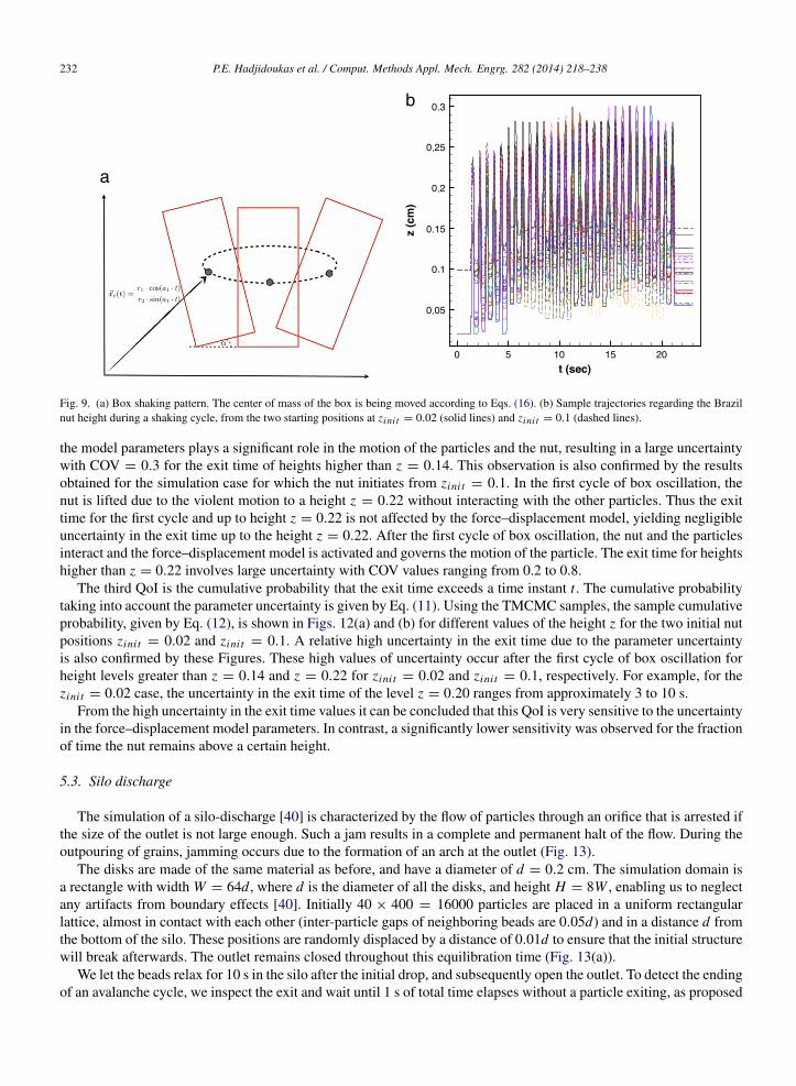
where xc(t) is the displacement of the center and α is the orientation angle of the box as seen in Fig. 9(a). The valuesof the parameters involved in (16) are fixed to r1 = 0.05, r2 = 0.083, a1 = 17 and a2 = 180 for the whole uncertaintypropagation procedure.

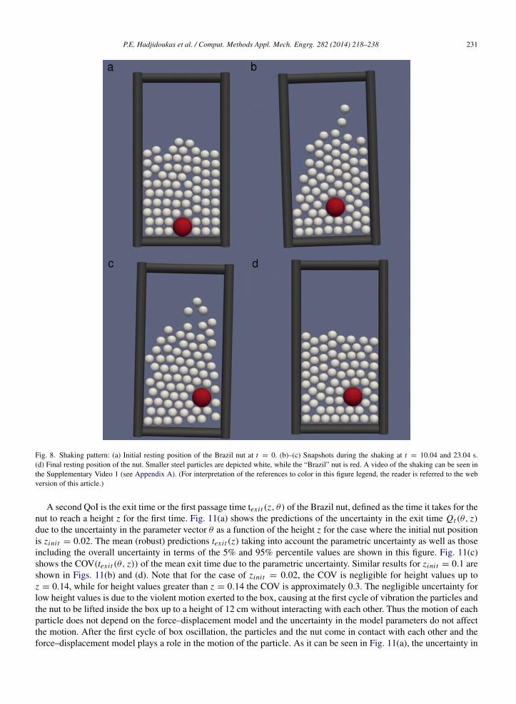
We define as p(z, θ) = t/t0 the fraction of time that the nut remains above a certain height z during a shakingthat lasts t0 seconds. The QoI is the height z p corresponding to a given value for p. Simulations of the system areperformed using the model class M3. Representative sample trajectories starting from two different initial points zini t ,located at the middle of the box at zini t = 0.02 and zini t = 0.1, are shown in Fig. 9(b). Fig. 8 shows 4 different phasesof the shaking procedure.

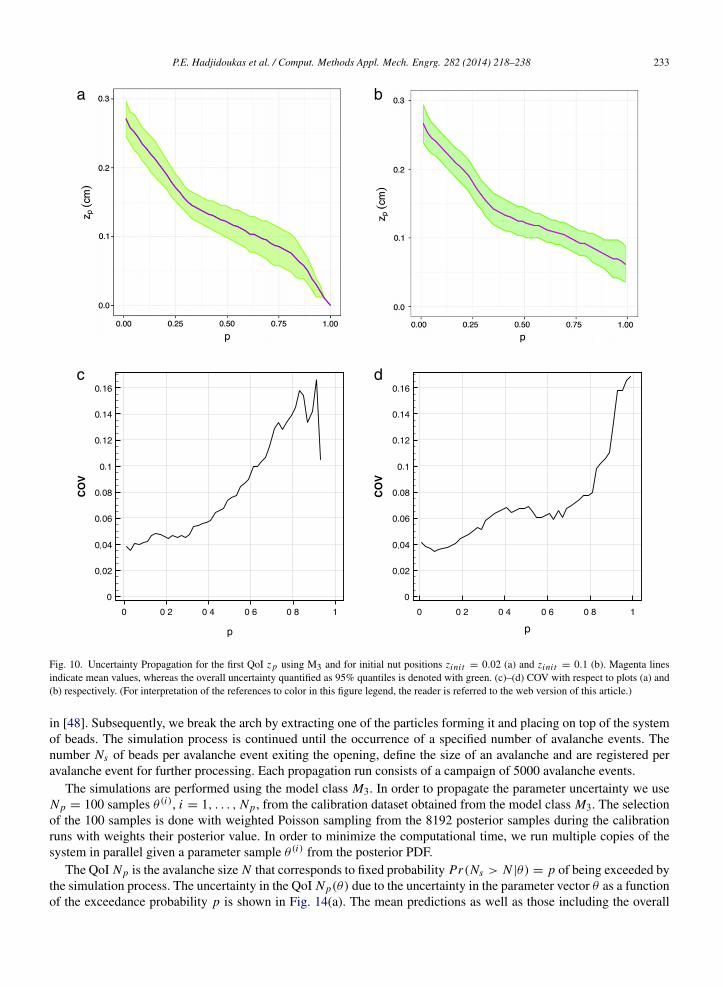
The uncertainty in the height z p(θ) as a function of the fraction of time p of exceeding the level z p(θ) is given inFigs. 10(a) and (b) for two initial positions of the nut at zini t = 0.02 and zini t = 0.1, respectively. The uncertainty isquantified by the mean value of the height z p(θ) with respect to θ , as well as the 5% and 95% credible intervals. Wehave used 500 samples of the posterior distribution in order to propagate parametric uncertainty. The selection of 500samples is done with weighted Poisson sampling from the 8192 posterior samples with their weight chosen to be theirposterior values. The COV (z p(θ)) of the height z p due to the parametric uncertainty is also shown in Figs. 10(c) and(d) for zini t = 0.02 and 0.1, respectively. As expected, the height z p is a decreasing function of the fraction of timep. From the values of the COV we remark the tendency for the uncertainty in z p to increase as the fraction of timep is increasing. The COV values for these two particular zini t simulation cases range from values as low as 4% forsmall fractions of time p to values as high as 16% for higher p values. It is clear that the uncertainty in the F–D modelparameter values has an effect on this particular QoI.


Fig. 8. Shaking pattern: (a) Initial resting position of the Brazil nut at t = 0. (b)–(c) Snapshots during the shaking at t = 10.04 and 23.04 s.(d) Final resting position of the nut. Smaller steel particles are depicted white, while the “Brazil” nut is red. A video of the shaking can be seen inthe Supplementary Video 1 (see Appendix A). (For interpretation of the references to color in this figure legend, the reader is referred to the webversion of this article.)

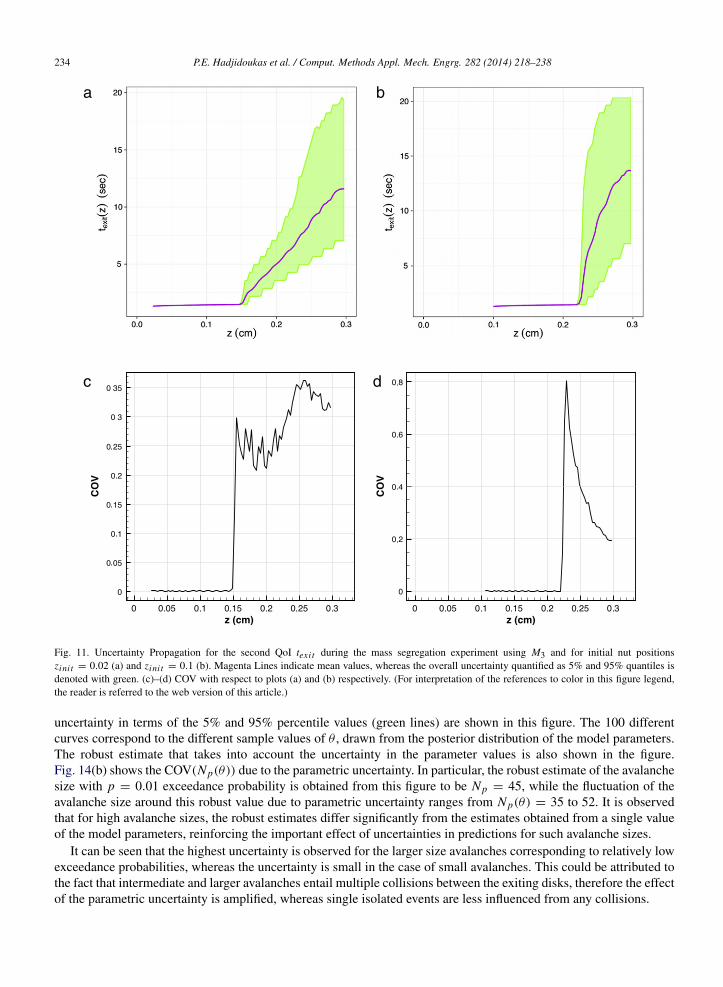
A second QoI is the exit time or the first passage time texi t (z, θ) of the Brazil nut, defined as the time it takes for thenut to reach a height z for the first time. Fig. 11(a) shows the predictions of the uncertainty in the exit time Qt (θ, z)due to the uncertainty in the parameter vector θ as a function of the height z for the case where the initial nut positionis zini t = 0.02. The mean (robust) predictions texi t (z) taking into account the parametric uncertainty as well as thoseincluding the overall uncertainty in terms of the 5% and 95% percentile values are shown in this figure. Fig. 11(c)shows the COV(texi t (θ, z)) of the mean exit time due to the parametric uncertainty. Similar results for zini t = 0.1 areshown in Figs. 11(b) and (d). Note that for the case of zini t = 0.02, the COV is negligible for height values up toz = 0.14, while for height values greater than z = 0.14 the COV is approximately 0.3. The negligible uncertainty forlow height values is due to the violent motion exerted to the box, causing at the first cycle of vibration the particles andthe nut to be lifted inside the box up to a height of 12 cm without interacting with each other. Thus the motion of eachparticle does not depend on the force–displacement model and the uncertainty in the model parameters do not affectthe motion. After the first cycle of box oscillation, the particles and the nut come in contact with each other and theforce–displacement model plays a role in the motion of the particle. As it can be seen in Fig. 11(a), the uncertainty in


Fig. 9. (a) Box shaking pattern. The center of mass of the box is being moved according to Eqs. (16). (b) Sample trajectories regarding the Brazilnut height during a shaking cycle, from the two starting positions at zini t = 0.02 (solid lines) and zini t = 0.1 (dashed lines).

the model parameters plays a significant role in the motion of the particles and the nut, resulting in a large uncertaintywith COV = 0.3 for the exit time of heights higher than z = 0.14. This observation is also confirmed by the resultsobtained for the simulation case for which the nut initiates from zini t = 0.1. In the first cycle of box oscillation, thenut is lifted due to the violent motion to a height z = 0.22 without interacting with the other particles. Thus the exittime for the first cycle and up to height z = 0.22 is not affected by the force–displacement model, yielding negligibleuncertainty in the exit time up to the height z = 0.22. After the first cycle of box oscillation, the nut and the particlesinteract and the force–displacement model is activated and governs the motion of the particle. The exit time for heightshigher than z = 0.22 involves large uncertainty with COV values ranging from 0.2 to 0.8.

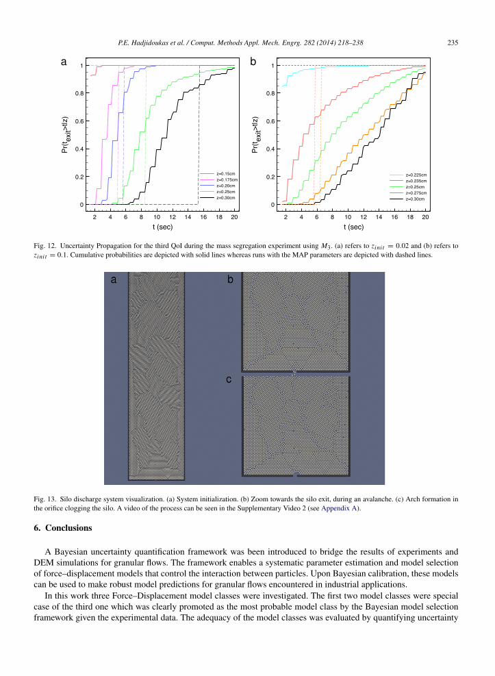
The third QoI is the cumulative probability that the exit time exceeds a time instant t . The cumulative probabilitytaking into account the parameter uncertainty is given by Eq. (11). Using the TMCMC samples, the sample cumulativeprobability, given by Eq. (12), is shown in Figs. 12(a) and (b) for different values of the height z for the two initial nutpositions zini t = 0.02 and zini t = 0.1. A relative high uncertainty in the exit time due to the parameter uncertaintyis also confirmed by these Figures. These high values of uncertainty occur after the first cycle of box oscillation forheight levels greater than z = 0.14 and z = 0.22 for zini t = 0.02 and zini t = 0.1, respectively. For example, for thezini t = 0.02 case, the uncertainty in the exit time of the level z = 0.20 ranges from approximately 3 to 10 s.

From the high uncertainty in the exit time values it can be concluded that this QoI is very sensitive to the uncertaintyin the force–displacement model parameters. In contrast, a significantly lower sensitivity was observed for the fractionof time the nut remains above a certain height.

5.3. Silo discharge

The simulation of a silo-discharge [40] is characterized by the flow of particles through an orifice that is arrested ifthe size of the outlet is not large enough. Such a jam results in a complete and permanent halt of the flow. During theoutpouring of grains, jamming occurs due to the formation of an arch at the outlet (Fig. 13).

The disks are made of the same material as before, and have a diameter of d = 0.2 cm. The simulation domain isa rectangle with width W = 64d, where d is the diameter of all the disks, and height H = 8W , enabling us to neglectany artifacts from boundary effects [40]. Initially 40 × 400 = 16000 particles are placed in a uniform rectangularlattice, almost in contact with each other (inter-particle gaps of neighboring beads are 0.05d) and in a distance d fromthe bottom of the silo. These positions are randomly displaced by a distance of 0.01d to ensure that the initial structurewill break afterwards. The outlet remains closed throughout this equilibration time (Fig. 13(a)).

We let the beads relax for 10 s in the silo after the initial drop, and subsequently open the outlet. To detect the endingof an avalanche cycle, we inspect the exit and wait until 1 s of total time elapses without a particle exiting, as proposed


a b

c d

Fig. 10. Uncertainty Propagation for the first QoI z p using M3 and for initial nut positions zini t = 0.02 (a) and zini t = 0.1 (b). Magenta linesindicate mean values, whereas the overall uncertainty quantified as 95% quantiles is denoted with green. (c)–(d) COV with respect to plots (a) and(b) respectively. (For interpretation of the references to color in this figure legend, the reader is referred to the web version of this article.)

in [48]. Subsequently, we break the arch by extracting one of the particles forming it and placing on top of the systemof beads. The simulation process is continued until the occurrence of a specified number of avalanche events. Thenumber Ns of beads per avalanche event exiting the opening, define the size of an avalanche and are registered peravalanche event for further processing. Each propagation run consists of a campaign of 5000 avalanche events.

The simulations are performed using the model class M3. In order to propagate the parameter uncertainty we useNp = 100 samples θ (i), i = 1, . . . , Np, from the calibration dataset obtained from the model class M3. The selectionof the 100 samples is done with weighted Poisson sampling from the 8192 posterior samples during the calibrationruns with weights their posterior value. In order to minimize the computational time, we run multiple copies of thesystem in parallel given a parameter sample θ (i) from the posterior PDF.

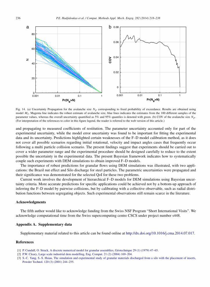
The QoI Np is the avalanche size N that corresponds to fixed probability Pr(Ns > N |θ) = p of being exceeded bythe simulation process. The uncertainty in the QoI Np(θ) due to the uncertainty in the parameter vector θ as a functionof the exceedance probability p is shown in Fig. 14(a). The mean predictions as well as those including the overall


a b

c d

Fig. 11. Uncertainty Propagation for the second QoI texi t during the mass segregation experiment using M3 and for initial nut positionszini t = 0.02 (a) and zini t = 0.1 (b). Magenta Lines indicate mean values, whereas the overall uncertainty quantified as 5% and 95% quantiles isdenoted with green. (c)–(d) COV with respect to plots (a) and (b) respectively. (For interpretation of the references to color in this figure legend,the reader is referred to the web version of this article.)

uncertainty in terms of the 5% and 95% percentile values (green lines) are shown in this figure. The 100 differentcurves correspond to the different sample values of θ , drawn from the posterior distribution of the model parameters.The robust estimate that takes into account the uncertainty in the parameter values is also shown in the figure.Fig. 14(b) shows the COV(Np(θ)) due to the parametric uncertainty. In particular, the robust estimate of the avalanchesize with p = 0.01 exceedance probability is obtained from this figure to be Np = 45, while the fluctuation of theavalanche size around this robust value due to parametric uncertainty ranges from Np(θ) = 35 to 52. It is observedthat for high avalanche sizes, the robust estimates differ significantly from the estimates obtained from a single valueof the model parameters, reinforcing the important effect of uncertainties in predictions for such avalanche sizes.

It can be seen that the highest uncertainty is observed for the larger size avalanches corresponding to relatively lowexceedance probabilities, whereas the uncertainty is small in the case of small avalanches. This could be attributed tothe fact that intermediate and larger avalanches entail multiple collisions between the exiting disks, therefore the effectof the parametric uncertainty is amplified, whereas single isolated events are less influenced from any collisions.


Fig. 12. Uncertainty Propagation for the third QoI during the mass segregation experiment using M3. (a) refers to zini t = 0.02 and (b) refers tozini t = 0.1. Cumulative probabilities are depicted with solid lines whereas runs with the MAP parameters are depicted with dashed lines.

Fig. 13. Silo discharge system visualization. (a) System initialization. (b) Zoom towards the silo exit, during an avalanche. (c) Arch formation inthe orifice clogging the silo. A video of the process can be seen in the Supplementary Video 2 (see Appendix A).

6. Conclusions

A Bayesian uncertainty quantification framework was been introduced to bridge the results of experiments andDEM simulations for granular flows. The framework enables a systematic parameter estimation and model selectionof force–displacement models that control the interaction between particles. Upon Bayesian calibration, these modelscan be used to make robust model predictions for granular flows encountered in industrial applications.

In this work three Force–Displacement model classes were investigated. The first two model classes were specialcase of the third one which was clearly promoted as the most probable model class by the Bayesian model selectionframework given the experimental data. The adequacy of the model classes was evaluated by quantifying uncertainty


a b

Fig. 14. (a) Uncertainty Propagation for the avalanche size Np corresponding to fixed probability of exceedance. Results are obtained usingmodel M3. Magenta line indicates the robust estimate of avalanche size, blue lines indicates the estimates from the 100 different samples of theparameter values, whereas the overall uncertainty quantified as 5% and 95% quantiles is denoted with green. (b) COV of the avalanche size Np .(For interpretation of the references to color in this figure legend, the reader is referred to the web version of this article.)

and propagating to measured coefficients of restitution. The parameter uncertainty accounted only for part of theexperimental uncertainty, while the model error uncertainty was found to be important for fitting the experimentaldata and its uncertainty. Predictions highlighted certain weaknesses of the F–D model calibration method, as it doesnot cover all possible scenarios regarding initial rotational, velocity and impact angles cases that frequently occurfollowing a multi particle collision scenario. The present findings suggest that experiments should be carried out tocover a wider parameter range and the experimental procedure should be designed carefully to reduce to the extentpossible the uncertainty in the experimental data. The present Bayesian framework indicates how to systematicallycouple such experiments with DEM simulations to obtain improved F–D models.

The importance of robust predictions for granular flows using DEM simulations was illustrated, with two appli-cations: the Brazil nut effect and Silo discharge for steel particles. The parametric uncertainties were propagated andtheir significance was demonstrated for the selected QoI for these two problems.

Current work involves the development of hierarchical F–D models for DEM simulations using Bayesian uncer-tainty criteria. More accurate predictions for specific applications could be achieved not by a bottom-up approach ofinferring the F–D model by pairwise collisions, but by calibrating with a collective observable, such as radial distri-bution functions between segregating objects. Such experimental observations still remain scarce in the literature.

Acknowledgments

The fifth author would like to acknowledge funding from the Swiss NSF Program “Short International Visits”. Weacknowledge computational time from the Swiss supercomputing centre CSCS under project number s448.

Appendix A. Supplementary data

Supplementary material related to this article can be found online at http://dx.doi.org/10.1016/j.cma.2014.07.017.

References

[1] P. Cundall, O. Strack, A discrete numerical model for granular assemblies, Geotechnique 29 (1) (1979) 47–65.[2] P.W. Cleary, Large scale industrial dem modelling, Eng. Comput. 21 (2) (2004) 169–204.[3] S.-C. Yang, S.-S. Hsiau, The simulation and experimental study of granular materials discharged from a silo with the placement of inserts,

Powder Technol. 120 (3) (2001) 244–255.


http://refhub.elsevier.com/S0045-7825(14)00249-7/sbref1




[4] T.J. Goda, F. Ebert, Three-dimensional discrete element simulations in hoppers and silos, Powder Technol. 158 (1–3) (2005) 58–68.[5] C. Gonzalez-Montellano, A. Ramırez, E. Gallego, F. Ayuga, Validation and experimental calibration of 3d discrete element models for the

simulation of the discharge flow in silos, Chem. Eng. Sci. 66 (21) (2011) 5116–5126.[6] P.A. Langston, U. Tuzun, D.M. Heyes, Discrete element simulation of granular flow in 2d and 3d hoppers: dependence of discharge rate and

wall stress on particle interactions, Chem. Eng. Sci. 50 (6) (1995) 967–987.[7] G. Marketos, C. O’Sullivan, A micromechanics-based analytical method for wave propagation through a granular material, Soil Dyn. Earthq.

Eng. 45 (2013) 25–34.[8] B. Peters, A. Dzuiugys, H. Hunsinger, L. Krebs, An approach to qualify the intensity of mixing on a forward acting grate, Chem. Eng. Sci. 60

(6) (2005) 1649–1659.[9] G.J. Finnie, N.P. Kruyt, M. Ye, C. Zeilstra, J.A.M. Kuipers, Longitudinal and transverse mixing in rotary kilns: a discrete element method

approach, Chem. Eng. Sci. 60 (15) (2005) 4083–4091.[10] H. Kruggel-Emden, E. Simsek, S. Wirtz, V. Scherer, A comparative numerical study of particle mixing on different grate designs through the

discrete element method, J. Press. Vessel Technol. 129 (4) (2007) 593–600.[11] Y. Tsuji, T. Kawaguchi, T. Tanaka, Discrete particle simulation of two-dimensional fluidized bed, Powder Technol. 77 (1) (1993) 79–87.[12] W. Zhong, Y. Xiong, Z. Yuan, M. Zhang, Dem simulation of gas–solid flow behaviors in spout-fluid bed, Chem. Eng. Sci. 61 (5) (2006)

1571–1584.[13] Y. Tsuji, Multi-scale modeling of dense phase gas–particle flow, Chem. Eng. Sci. 62 (13) (2007) 3410–3418.[14] H.P. Kuo, P.C. Knight, D.J. Parker, Y. Tsuji, M.J. Adams, J.P.K. Seville, The influence of dem simulation parameters on the particle behaviour

in a v-mixer, Chem. Eng. Sci. 57 (17) (2002) 3621–3638.[15] E. Dintwa, M. Van Zeebroeck, E. Tijskens, H. Ramon, Determination of parameters of a tangential contact force model for viscoelastic

spheroids (fruits) using a rheometer device, Biosystems Eng. 91 (3) (2005) 321–327.[16] C.J. Coetzee, D.N.J. Els, Calibration of discrete element parameters and the modelling of silo discharge and bucket filling, Comput. Electron.

Agric. 65 (2) (2009) 198–212.[17] E. Alizadeh, F. Bertrand, J. Chaouki, Development of a granular normal contact force model based on a non-newtonian liquid filled dashpot,

Powder Technol. 237 (2013) 202–212.[18] F.P. Di Maio, A. Di Renzo, Modelling particle contacts in distinct element simulations: linear and non-linear approach, Chem. Eng. Res. Des.

83 (11) (2005) 1287–1297.[19] H. Kruggel-Emden, S. Wirtz, V. Scherer, A study on tangential force laws applicable to the discrete element method (dem) for materials with

viscoelastic or plastic behavior, Chem. Eng. Sci. 63 (6) (2008) 1523–1541.[20] J.L. Beck, K.-V. Yuen, Model selection using response measurements: Bayesian probabilistic approach, J. Eng. Mech. 130 (2) (2004) 192–203.[21] J.T. Oden, A. Hawkins, S. Prudhomme, General diffuse interface theories and an approach to predictive tumor growth modeling, Math. Models

Methods Appl. Sci. 20 (3) (2010) 477–517.[22] K.-V. Yuen, Bayesian Methods for Structural Dynamics and Civil Engineering, Wiley-Vch Verlag, 2010.[23] J.L. Beck, S.K. Au, Bayesian updating of structural models and reliability using Markov chain monte carlo simulation, J. Eng. Mech. 128 (4)

(2002) 380–391.[24] X. Ma, N. Zabaras, A stochastic mixed finite element heterogeneous multiscale method for flow in porous media, J. Comput. Phys. 230 (12)

(2011) 4696–4722.[25] S.H. Cheung, T.A. Oliver, E.E. Prudencio, S. Prudhomme, R.D. Moser, Bayesian uncertainty analysis with applications to turbulence

modeling, Rel. Eng. Sys. Saf. 96 (9) (2011) 1137–1149.[26] P.M. Congedo, P. Colonna, C. Corre, J.A.S. Witteveen, G. Iaccarino, Backward uncertainty propagation method in flow problems: application

to the prediction of rarefaction shock waves, Comp. Meth. Appl. Sci. Eng. 213–216 (2012) 314–326.[27] P.L. Garrido, J. Marro, H.J. Herrmann, 3rd Granada Lectures in Computational Physics, vol. 448, Springer, Berlin, Heidelberg, 1995,

pp. 67–114 (Chapter 2).[28] J. Ching, Y.C. Chen, Transitional Markov chain monte carlo method for Bayesian model updating, model class selection, and model averaging,

J. Eng. Mech. 133 (7) (2007) 816–832.[29] P. Angelikopoulos, C. Papadimitriou, P. Koumoutsakos, Bayesian uncertainty quantification and propagation in molecular dynamics

simulations: a high performance computing framework, J. Chem. Phys. 137 (14) (2012) 144103.[30] P.E. Hadjidoukas, E. Lappas, V.V. Dimakopoulos, A runtime library for platform-independent task parallelism, in: 20th Euromicro

International Conference on Parallel, Distributed and Network-Based Processing (PDP), IEEE Computer Society, Munich, Germany, 2012,pp. 229–236.

[31] T. Poschel, T. Schwager, Computational Granular Dynamics—Models and Algorithms, Springer-Verlag, New York, 2005.[32] H. Kruggel-Emden, M. Sturm, S. Wirtz, V. Scherer, Selection of an appropriate time integration scheme for the discrete element method

(dem), Comput. Chem. Eng. 32 (10) (2008) 2263–2279.[33] H. Hertz, Ueber die beruhrung fester elastischer korper, J. Reine Angew. Math. 1882 (1882) 156.[34] S. Timoshenko, J.N. Goodier, Theory of elasticity, in: Engineering Societies Monographs, McGraw-Hill, New York, 1969.[35] H. Kruggel-Emden, F. Stepanek, A. Munjiza, Performance of integration schemes in discrete element simulations of particle systems involving

consecutive contacts, Comput. Chem. Eng. 35 (10) (2011) 2152–2157.[36] Y. Tsuji, T. Tanaka, T. Ishida, Lagrangian numerical simulation of plug flow of cohesionless particles in a horizontal pipe, Powder Technol.

71 (3) (1992) 239–250.[37] G. Kuwabara, K. Kono, Restitution coefficient in a collision between two spheres, Japan. J. Appl. Phys. 26 (1987) 1230–1233. Part 1, No. 8.[38] N.V. Brilliantov, F. Spahn, J.-M. Hertzsch, T. Poschel, Model for collisions in granular gases, Phys. Rev. E 53 (1996) 5382–5392.[39] L. Brendel, S. Dippel, Lasting contacts in molecular dynamics simulations, in: Physics of Dry Granular Media, Kluwer Academic Publishers,

1998, pp. 31–33.






































[40] D. Hirshfeld, D. Rapaport, Granular flow from a silo: discrete-particle simulations in three dimensions, Eur. Phys. J. E 4 (2) (2001) 193–199.[41] H. Jeffreys, Theory of Probability, third ed., Oxford University Press, USA, 1961.[42] E. Simoen, C. Papadimitriou, G. Lombaert, On prediction error correlation in Bayesian model updating, J. Sound Vib. 332 (18) (2013)

4136–4152.[43] A. Doucet, N. De Freitas, N. Gordon, Sequential Monte Carlo Methods in Practice, Springer, 2001.[44] C. Papadimitriou, J.L. Beck, L.S. Katafygiotis, Updating robust reliability using structural test data, Prob. Eng. Mech. 16 (2) (2001) 103–113.[45] A. Taflanidis, J.L. Beck, Prior and posterior robust stochastic predictions for dynamical systems using probability logic, Int. J. Unc. Qu. 3 (4)

(2013) 271–288.[46] H. Dong, M.H. Moys, Experimental study of oblique impacts with initial spin, Powder Technol. 161 (1) (2006) 22–31.[47] T. Schwager, V. Becker, T. Poschel, Coefficient of tangential restitution for viscoelastic spheres, Eur. Phys. J. E 27 (1) (2008) 107–114.[48] I. Zuriguel, A. Garcimartın, D. Maza, L. Pugnaloni, J. Pastor, Jamming during the discharge of granular matter from a silo, Phys. Rev. E 71

(2005) 051303.










Documents

Bayesian uncertainty quantification and …Bayesian uncertainty quantification and propagation for the DEM We consider a parametrized class M of a Force–Displacement model, and let