Embed Size (px)
Citation preview
Bayesian Vector Autoregressions
Lawrence J. Christiano
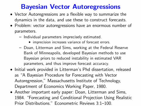
Bayesian Vector Autoregressions• Vector Autoregressions are a flexible way to summarize thedynamics in the data, and use these to construct forecasts.
• Problem: vector autoregressions have an enormous number ofparameters.— Individual parameters imprecisely estimated.
• imprecision increases variance of forecast errors.— Doan, Litterman and Sims, working at the Federal ReserveBank of Minneapolis, developed Bayesian methods to useBayesian priors to reduced instability in estimated VARparameters, and thus improve forecast accuracy.
• Initial work provided in Litterman’s Phd dissertation, releasedas “A Bayesian Procedure for Forecasting with VectorAutoregression,”Massachusetts Institute of Technology,Department of Economics Working Paper, 1980.
• Another important early paper: Doan, Litterman and Sims,1984. “Forecasting and Conditional Projection Using RealisticPrior Distributions.”Econometric Reviews 3:1—100.
Bayesian Vector Autoregressions
• Of course, much has been written to describe BVARs.— Classic treatment: Arnold Zellner, An Introduction to BayesianInference in Econometrics, John Wiley & Sons, 1971.
— Hamilton’s textbook, Time Series Analysis has a very goodchapter.
— Here is an accessible discussion: Robertson and Tallman,‘Vectors Autoregressions: Forecasting and Reality’, FederalReserve Bank of Atlanta, Economic Reviews, First Quarter,1999.
— Rigorous recent reviews of the subject: Del Negro andSchorfheide, ‘Bayesian Macroeconometrics,’chapter inHandbook Bayesian Econometrics, Oxford University Press,2011.
Outline• Normal Likelihood, Illustrated with Simple AR(2)representation.— conditional versus unconditional likelihood.— maximum likelihood with level GDP data.— the Hurwicz bias.
• Three representations of a VAR.— Standard Representation— Matrix Representation— Vectorized Representation.
• Priors, posteriors and marginal likelihood— Dummy observations.— Conjugate Priors.
• Forecasting with BVARs— stochastic simulations, versus non-stochastic.— forecast probability intervals.
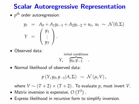
Scalar Autoregressive Representation• pth order autoregression:
yt = A0 +A1yt−1 +A2yt−2 + ut, ut ∼ N (0, Σ)
Y =
y1...
yT
.
• Observed data:
Y,initial conditions︷ ︸︸ ︷
y0, y−1 .
• Normal likelihood of observed data:
p (Y, y0, y−1|A, Σ) ∼ N (µ, V) ,
where V ∼ (T+ 2)× (T+ 2) . To evaluate p, must invert V.• Matrix inversion is expensive, O
(T3) .
• Express likelihood in recursive form to simplify inversion.
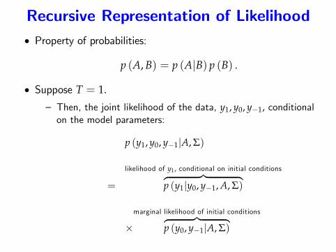
Recursive Representation of Likelihood• Property of probabilities:
p (A, B) = p (A|B) p (B) .
• Suppose T = 1.
— Then, the joint likelihood of the data, y1, y0, y−1, conditionalon the model parameters:
p (y1, y0, y−1|A, Σ)
=
likelihood of y1, conditional on initial conditions︷ ︸︸ ︷p (y1|y0, y−1, A, Σ)
×marginal likelihood of initial conditions︷ ︸︸ ︷
p (y0, y−1|A, Σ)
Recursive Representation of Likelihood
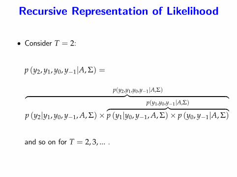
• Consider T = 2:
p (y2, y1, y0, y−1|A, Σ) =
p(y2,y1,y0,y−1|A,Σ)︷ ︸︸ ︷p (y2|y1, y0, y−1, A, Σ)×
p(y1,y0,y−1|A,Σ)︷ ︸︸ ︷p (y1|y0, y−1, A, Σ)× p (y0, y−1|A, Σ) ,
and so on for T = 2, 3, ... .
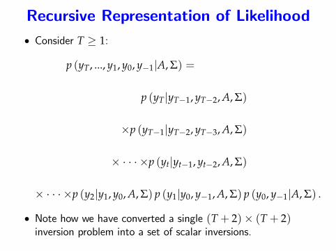
Recursive Representation of Likelihood• Consider T ≥ 1:
p (yT, ..., y1, y0, y−1|A, Σ) =
p (yT|yT−1, yT−2, A, Σ)
×p (yT−1|yT−2, yT−3, A, Σ)
× · · · ×p (yt|yt−1, yt−2, A, Σ)
× · · · ×p (y2|y1, y0, A, Σ) p (y1|y0, y−1, A, Σ) p (y0, y−1|A, Σ) .
• Note how we have converted a single (T+ 2)× (T+ 2)inversion problem into a set of scalar inversions.
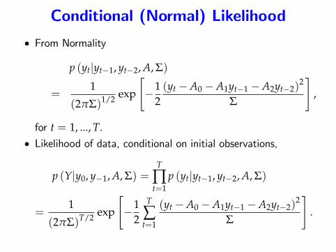
Conditional (Normal) Likelihood
• From Normality
p (yt|yt−1, yt−2, A, Σ)
=1
(2πΣ)1/2 exp
[−1
2(yt −A0 −A1yt−1 −A2yt−2)
2
Σ
],
for t = 1, ..., T.• Likelihood of data, conditional on initial observations,
p (Y|y0, y−1, A, Σ) =T
∏t=1
p (yt|yt−1, yt−2, A, Σ)
=1
(2πΣ)T/2 exp
[−1
2
T
∑t=1
(yt −A0 −A1yt−1 −A2yt−2)2
Σ
].
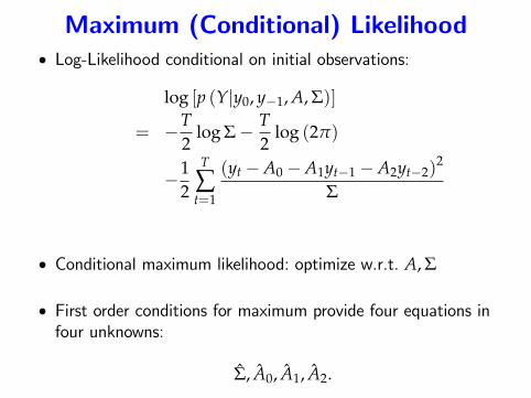
Maximum (Conditional) Likelihood• Log-Likelihood conditional on initial observations:
log [p (Y|y0, y−1, A, Σ)]
= −T2
log Σ− T2
log (2π)
−12
T
∑t=1
(yt −A0 −A1yt−1 −A2yt−2)2
Σ
• Conditional maximum likelihood: optimize w.r.t. A, Σ
• First order conditions for maximum provide four equations infour unknowns:
Σ, A0, A1, A2.
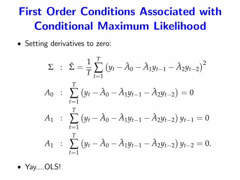
First Order Conditions Associated withConditional Maximum Likelihood
• Setting derivatives to zero:
Σ : Σ =1T
T
∑t=1
(yt − A0 − A1yt−1 − A2yt−2
)2
A0 :T
∑t=1
(yt − A0 − A1yt−1 − A2yt−2
)= 0
A1 :T
∑t=1
(yt − A0 − A1yt−1 − A2yt−2
)yt−1 = 0
A1 :T
∑t=1
(yt − A0 − A1yt−1 − A2yt−2
)yt−2 = 0.
• Yay....OLS!
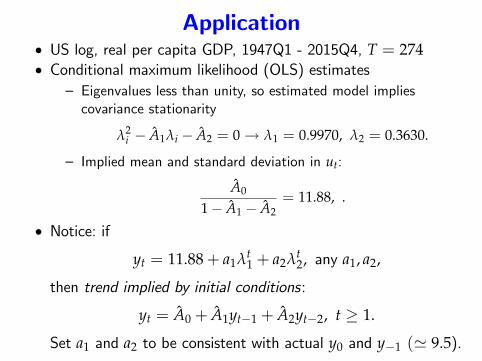
Application• US log, real per capita GDP, 1947Q1 - 2015Q4, T = 274• Conditional maximum likelihood (OLS) estimates
— Eigenvalues less than unity, so estimated model impliescovariance stationarity
λ2i − A1λi − A2 = 0→ λ1 = 0.9970, λ2 = 0.3630.
— Implied mean and standard deviation in ut:
A0
1− A1 − A2= 11.88, .
• Notice: if
yt = 11.88+ a1λt1 + a2λt
2, any a1, a2,
then trend implied by initial conditions:
yt = A0 + A1yt−1 + A2yt−2, t ≥ 1.
Set a1 and a2 to be consistent with actual y0 and y−1 (' 9.5).
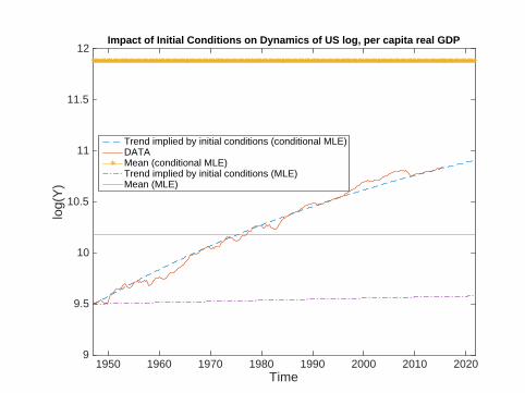
Time1950 1960 1970 1980 1990 2000 2010 2020
log(
Y)
9
9.5
10
10.5
11
11.5
12Impact of Initial Conditions on Dynamics of US log, per capita real GDP
Trend implied by initial conditions (conditional MLE)DATAMean (conditional MLE)Trend implied by initial conditions (MLE)Mean (MLE)
Message of Application
• Illustrates how maximum of conditional likelihood is computedby OLS.
• Maximum of conditional likelihood with growing data.— tends to ‘explain’data as emerging from covariance stationarymodel (roots inside unit circle).
• related to ‘Hurwicz bias’, tendency for roots of VAR to shrinktowards zero.
— interprets growth as reflecting transition from unusual initialconditions.
• initial conditions account for a very large portion of datadynamics (see previous figure).
• most researchers view this as implausible.
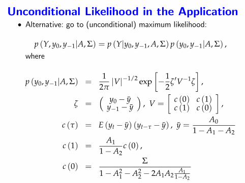
Unconditional Likelihood in the Application• Alternative: go to (unconditional) maximum likelihood:
p (Y, y0, y−1|A, Σ) = p (Y|y0, y−1, A, Σ) p (y0, y−1|A, Σ) ,where
p (y0, y−1|A, Σ) =1
2π|V|−1/2 exp
[−1
2ζ ′V−1ζ
],
ζ =( y0 − y
y−1 − y)
, V =
[c (0) c (1)c (1) c (0)
],
c (τ) = E (yt − y) (yt−τ − y) , y =A0
1−A1 −A2
c (1) =A1
1−A2c (0) ,
c (0) =Σ
1−A21 −A2
2 − 2A1A2A1
1−A2
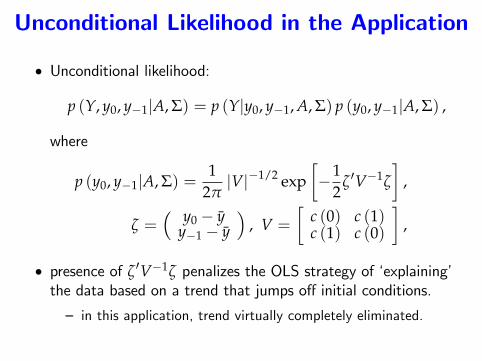
Unconditional Likelihood in the Application
• Unconditional likelihood:
p (Y, y0, y−1|A, Σ) = p (Y|y0, y−1, A, Σ) p (y0, y−1|A, Σ) ,
where
p (y0, y−1|A, Σ) =1
2π|V|−1/2 exp
[−1
2ζ ′V−1ζ
],
ζ =( y0 − y
y−1 − y)
, V =
[c (0) c (1)c (1) c (0)
],
• presence of ζ ′V−1ζ penalizes the OLS strategy of ‘explaining’the data based on a trend that jumps off initial conditions.
— in this application, trend virtually completely eliminated.
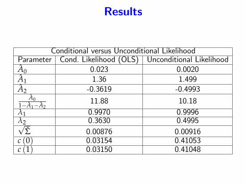
Results
Conditional versus Unconditional LikelihoodParameter Cond. Likelihood (OLS) Unconditional LikelihoodA0 0.023 0.0020A1 1.36 1.499A2 -0.3619 -0.4993
A01−A1−A2
11.88 10.18λ1 0.9970 0.9996λ2 0.3630 0.4995√
Σ 0.00876 0.00916c (0) 0.03154 0.41053c (1) 0.03150 0.41048
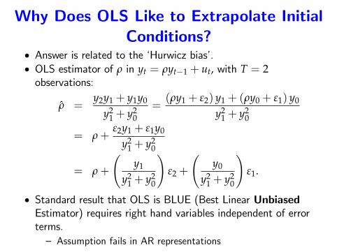
Why Does OLS Like to Extrapolate InitialConditions?
• Answer is related to the ‘Hurwicz bias’.• OLS estimator of ρ in yt = ρyt−1 + ut, with T = 2observations:
ρ =y2y1 + y1y0
y21 + y2
0=(ρy1 + ε2) y1 + (ρy0 + ε1) y0
y21 + y2
0
= ρ+ε2y1 + ε1y0
y21 + y2
0
= ρ+
(y1
y21 + y2
0
)ε2 +
(y0
y21 + y2
0
)ε1.
• Standard result that OLS is BLUE (Best Linear UnbiasedEstimator) requires right hand variables independent of errorterms.— Assumption fails in AR representations
Why Does OLS Like to Extrapolate InitialConditions?
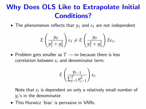
• The phenomenon reflects that y1 and ε1 are not independent
E
(y0
y21 + y2
0
)ε1 6= E
(y0
y21 + y2
0
)Eε1.
• Problem gets smaller as T → ∞ because there is lesscorrelation between εt and denominator term:
E
(yt−1
∑Tj=1 y2
j−1
)εt.
Note that εt is dependent on only a relatively small number ofyj’s in the denominator.
• This Hurwicz ‘bias’is pervasive in VARs.
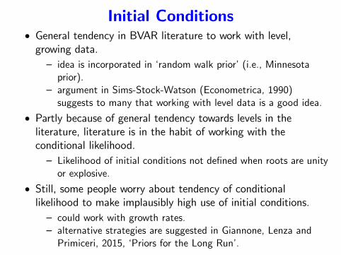
Initial Conditions• General tendency in BVAR literature to work with level,growing data.— idea is incorporated in ‘random walk prior’(i.e., Minnesotaprior).
— argument in Sims-Stock-Watson (Econometrica, 1990)suggests to many that working with level data is a good idea.
• Partly because of general tendency towards levels in theliterature, literature is in the habit of working with theconditional likelihood.— Likelihood of initial conditions not defined when roots are unityor explosive.
• Still, some people worry about tendency of conditionallikelihood to make implausibly high use of initial conditions.— could work with growth rates.— alternative strategies are suggested in Giannone, Lenza andPrimiceri, 2015, ‘Priors for the Long Run’.
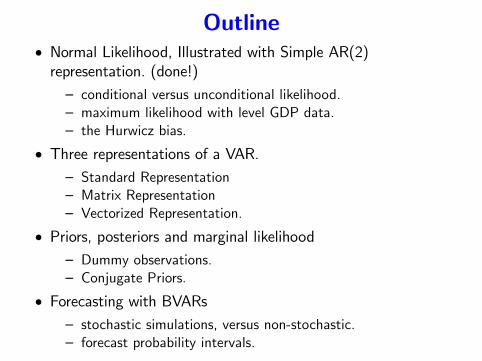
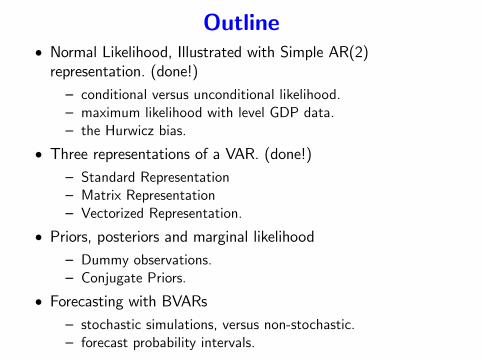
Outline• Normal Likelihood, Illustrated with Simple AR(2)representation. (done!)— conditional versus unconditional likelihood.— maximum likelihood with level GDP data.— the Hurwicz bias.
• Three representations of a VAR.— Standard Representation— Matrix Representation— Vectorized Representation.
• Priors, posteriors and marginal likelihood— Dummy observations.— Conjugate Priors.
• Forecasting with BVARs— stochastic simulations, versus non-stochastic.— forecast probability intervals.
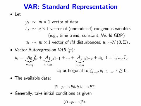
VAR: Standard Representation• Let
yt ∼ m× 1 vector of dataζt ∼ q× 1 vector of (unmodeled) exogenous variables
(e.g., time trend, constant, World GDP)
ut ∼ m× 1 vector of iid disturbances, ut ∼N (0, Σ) .
• Vector Autoregression VAR (p):
yt = A0︸︷︷︸m×q
ξt + A1︸︷︷︸m×m
yt−1 + ...+ Ap︸︷︷︸m×m
yt−p + ut, t = 1, ..., T,
ut orthogonal to ξt−s, yt−1−s, s ≥ 0.
• The available data:
y1−p, ..., y0, y1, ...., yT.
• Generally, take initial conditions as given
y1−p, ..., y0.
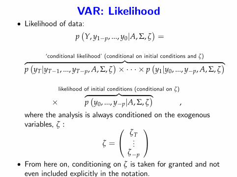
VAR: Likelihood• Likelihood of data:
p(Y, y1−p, ..., y0|A, Σ, ζ
)=
‘conditional likelihood’(conditional on initial conditions and ζ)︷ ︸︸ ︷p(yT|yT−1, ..., yT−p, A, Σ, ζ
)× · · · × p
(y1|y0, ..., y−p, A, Σ, ζ
)
×likelihood of initial conditions (conditional on ζ)︷ ︸︸ ︷
p(y0, ..., y−p|A, Σ, ζ
),
where the analysis is always conditioned on the exogenousvariables, ζ :
ζ =
ζT...
ζ−p
• From here on, conditioning on ζ is taken for granted and noteven included explicitly in the notation.
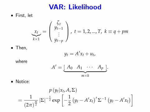
VAR: Likelihood• First, let
xt︸︷︷︸k×1
=
ζt
yt−1...
yt−p
, t = 1, 2, ..., T, k ≡ q+ pm
• Then,yt = A′xt + ut,
whereA′ = [ A0 A1 · · · Ap ]︸ ︷︷ ︸
m×k
.
• Notice:
p (yt|xt, A, Σ)
=1
(2π)m2|Σ|−
12 exp
[−1
2(yt −A′xt
)′ Σ−1 (yt −A′xt)]
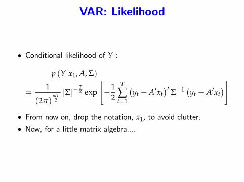
VAR: Likelihood
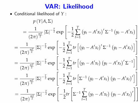
• Conditional likelihood of Y :
p (Y|x1, A, Σ)
=1
(2π)mT2|Σ|−
T2 exp
[−1
2
T
∑t=1
(yt −A′xt
)′ Σ−1 (yt −A′xt)]
• From now on, drop the notation, x1, to avoid clutter.• Now, for a little matrix algebra....
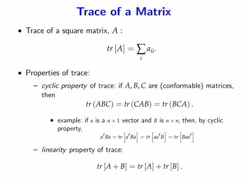
Trace of a Matrix• Trace of a square matrix, A :
tr [A] = ∑i
aii.
• Properties of trace:— cyclic property of trace: if A, B, C are (conformable) matrices,then
tr (ABC) = tr (CAB) = tr (BCA) .
• example: if a is a n× 1 vector and B is n× n, then, by cyclicproperty,
a′Ba = tr[a′Ba
]= tr
[aa′B
]= tr
[Baa′
]— linearity property of trace:
tr [A+ B] = tr [A] + tr [B] .
VAR: Likelihood• Conditional likelihood of Y :
p (Y|A, Σ)
=1
(2π)mT2|Σ|−
T2 exp
[−1
2
T
∑t=1
(yt −A′xt
)′ Σ−1 (yt −A′xt)]
=1
(2π)mT2|Σ|−
T2 exp
[−1
2
T
∑t=1
tr[(
yt −A′xt)′ Σ−1 (yt −A′xt
)]]
=1
(2π)mT2|Σ|−
T2 exp
[−1
2
T
∑t=1
tr[(
yt −A′xt) (
yt −A′xt)′ Σ−1
]]
=1
(2π)mT2|Σ|−
T2 exp
[−1
2
T
∑t=1
tr[Σ−1 (yt −A′xt
) (yt −A′xt
)′]]
=1
(2π)mT2|Σ|−
T2 exp
[−1
2tr
[Σ−1
T
∑t=1
(yt −A′xt
) (yt −A′xt
)′]]
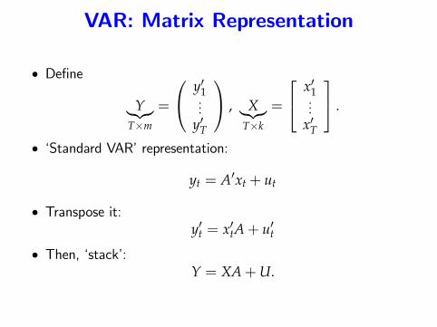
VAR: Matrix Representation
• Define
Y︸︷︷︸T×m
=
y′1...
y′T
, X︸︷︷︸T×k
=
x′1...
x′T
.
• ‘Standard VAR’representation:
yt = A′xt + ut
• Transpose it:y′t = x′tA+ u′t
• Then, ‘stack’:Y = XA+U.
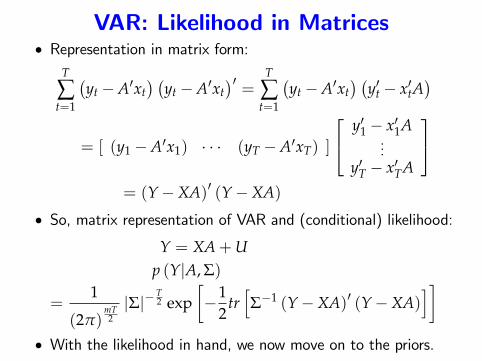
VAR: Likelihood in Matrices• Representation in matrix form:
T
∑t=1
(yt −A′xt
) (yt −A′xt
)′=
T
∑t=1
(yt −A′xt
) (y′t − x′tA
)= [ (y1 −A′x1) · · · (yT −A′xT) ]
y′1 − x′1A...
y′T − x′TA
= (Y−XA)′ (Y−XA)
• So, matrix representation of VAR and (conditional) likelihood:
Y = XA+Up (Y|A, Σ)
=1
(2π)mT2|Σ|−
T2 exp
[−1
2tr[Σ−1 (Y−XA)′ (Y−XA)
]]• With the likelihood in hand, we now move on to the priors.
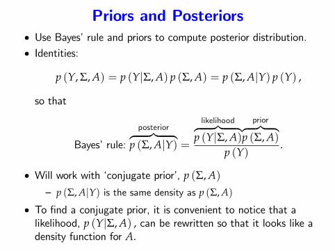
Priors and Posteriors• Use Bayes’rule and priors to compute posterior distribution.• Identities:
p (Y, Σ, A) = p (Y|Σ, A) p (Σ, A) = p (Σ, A|Y) p (Y) ,
so that
Bayes’rule:
posterior︷ ︸︸ ︷p (Σ, A|Y) =
likelihood︷ ︸︸ ︷p (Y|Σ, A)
prior︷ ︸︸ ︷p (Σ, A)
p (Y).
• Will work with ‘conjugate prior’, p (Σ, A)— p (Σ, A|Y) is the same density as p (Σ, A)
• To find a conjugate prior, it is convenient to notice that alikelihood, p (Y|Σ, A) , can be rewritten so that it looks like adensity function for A.
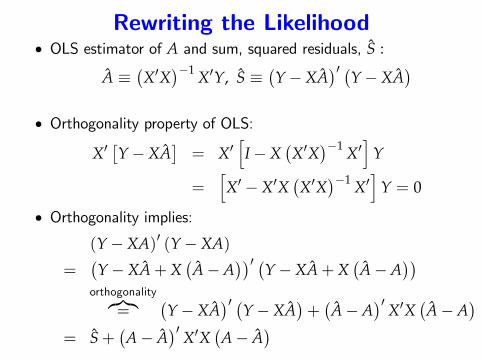
Rewriting the Likelihood• OLS estimator of A and sum, squared residuals, S :
A ≡(X′X
)−1 X′Y, S ≡(Y−XA
)′ (Y−XA)
• Orthogonality property of OLS:
X′[Y−XA
]= X′
[I−X
(X′X
)−1 X′]
Y
=[X′ −X′X
(X′X
)−1 X′]
Y = 0
• Orthogonality implies:
(Y−XA)′ (Y−XA)
=(Y−XA+X
(A−A
))′ (Y−XA+X(A−A
))orthogonality︷︸︸︷
=(Y−XA
)′ (Y−XA)+(A−A
)′ X′X (A−A)
= S+(A− A
)′ X′X (A− A)
Rewriting the Likelihood
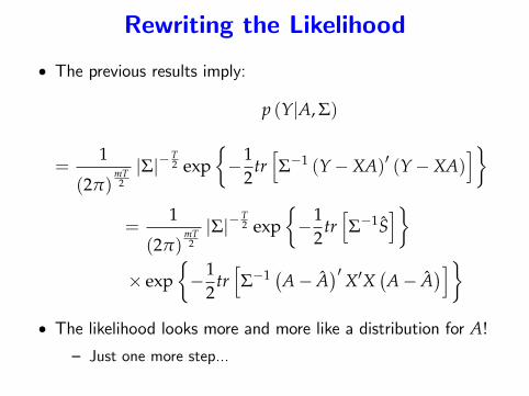
• The previous results imply:
p (Y|A, Σ)
=1
(2π)mT2|Σ|−
T2 exp
{−1
2tr[Σ−1 (Y−XA)′ (Y−XA)
]}
=1
(2π)mT2|Σ|−
T2 exp
{−1
2tr[Σ−1S
]}× exp
{−1
2tr[Σ−1 (A− A
)′ X′X (A− A)]}
• The likelihood looks more and more like a distribution for A!
— Just one more step...
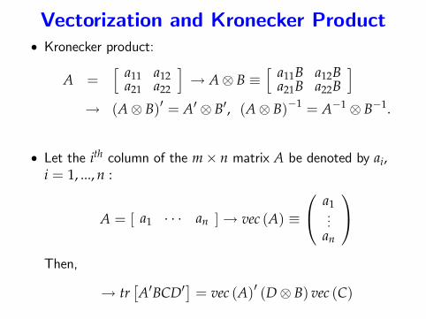
Vectorization and Kronecker Product• Kronecker product:
A =[ a11 a12
a21 a22
]→ A⊗ B ≡
[ a11B a12Ba21B a22B
]→ (A⊗ B)′ = A′ ⊗ B′, (A⊗ B)−1 = A−1 ⊗ B−1.
• Let the ith column of the m× n matrix A be denoted by ai,i = 1, ..., n :
A = [ a1 · · · an ]→ vec (A) ≡
a1...
an
Then,
→ tr[A′BCD′
]= vec (A)′ (D⊗ B) vec (C)
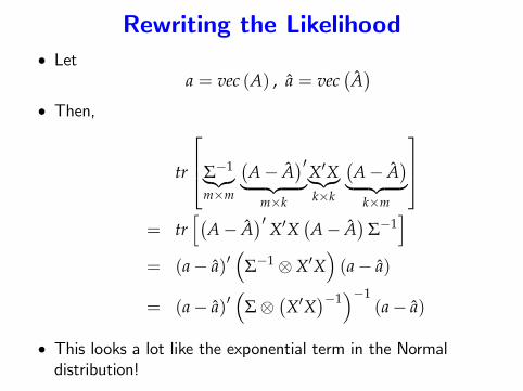
Rewriting the Likelihood• Let
a = vec (A) , a = vec(A)
• Then,
tr
Σ−1︸︷︷︸m×m
(A− A
)′︸ ︷︷ ︸m×k
X′X︸︷︷︸k×k
(A− A
)︸ ︷︷ ︸k×m
= tr
[(A− A
)′ X′X (A− A)
Σ−1]
= (a− a)′(
Σ−1 ⊗X′X)(a− a)
= (a− a)′(
Σ⊗(X′X
)−1)−1
(a− a)
• This looks a lot like the exponential term in the Normaldistribution!
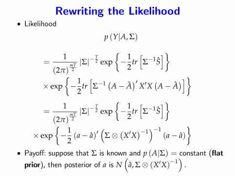
Rewriting the Likelihood• Likelihood
p (Y|A, Σ)
=1
(2π)mT2|Σ|−
T2 exp
{−1
2tr[Σ−1S
]}× exp
{−1
2tr[Σ−1 (A− A
)′ X′X (A− A)]}
=1
(2π)mT2|Σ|−
T2 exp
{−1
2tr[Σ−1S
]}× exp
{−1
2(a− a)′
(Σ⊗
(X′X
)−1)−1
(a− a)}
• Payoff: suppose that Σ is known and p (A|Σ) = constant (flatprior), then posterior of a is N
(a, Σ⊗ (X′X)−1
).
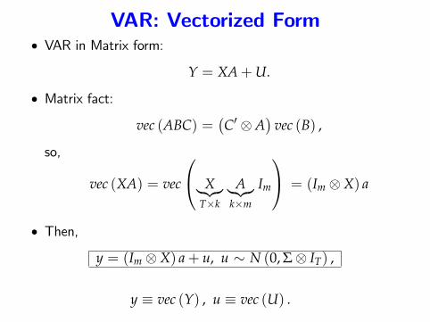
VAR: Vectorized Form• VAR in Matrix form:
Y = XA+U.
• Matrix fact:
vec (ABC) =(C′ ⊗A
)vec (B) ,
so,
vec (XA) = vec
X︸︷︷︸T×k
A︸︷︷︸k×m
Im
= (Im ⊗X) a
• Then,
y = (Im ⊗X) a+ u, u ∼ N (0, Σ⊗ IT) ,
y ≡ vec (Y) , u ≡ vec (U) .
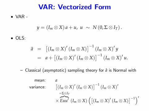
VAR: Vectorized Form• VAR -
y = (Im ⊗X) a+ u, u ∼ N (0, Σ⊗ IT) .
• OLS:
a =[(Im ⊗X)′ (Im ⊗X)
]−1(Im ⊗X)′ y
= a+[(Im ⊗X)′ (Im ⊗X)
]−1(Im ⊗X)′ u.
— Classical (asymptotic) sampling theory for a is Normal with
mean: avariance:
[(Im ⊗X)′ (Im ⊗X)
]−1(Im ⊗X)′
×=Σ⊗IT︷︸︸︷Euu′ (Im ⊗X)
([(Im ⊗X)′ (Im ⊗X)
]−1)′
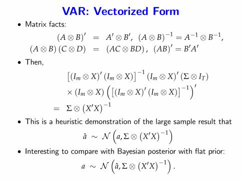
VAR: Vectorized Form• Matrix facts:
(A⊗ B)′ = A′ ⊗ B′, (A⊗ B)−1 = A−1 ⊗ B−1,(A⊗ B) (C⊗D) = (AC⊗ BD) , (AB)′ = B′A′
• Then, [(Im ⊗X)′ (Im ⊗X)
]−1(Im ⊗X)′ (Σ⊗ IT)
× (Im ⊗X)([(Im ⊗X)′ (Im ⊗X)
]−1)′
= Σ⊗(X′X
)−1
• This is a heuristic demonstration of the large sample result that
a ∼ N(
a, Σ⊗(X′X
)−1)
• Interesting to compare with Bayesian posterior with flat prior:
a ∼ N(
a, Σ⊗(X′X
)−1)
.
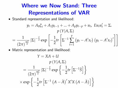
Where we Now Stand: ThreeRepresentations of VAR
• Standard representation and likelihood:
yt = A0ξt +A1yt−1 + ...+Apyt−p + ut, Eutu′t = Σ.p (Y|A, Σ)
=1
(2π)mT2|Σ|−
T2 exp
[−1
2tr
[Σ−1
T
∑t=1
(yt −A′xt
) (yt −A′xt
)′]]• Matrix representation and likelihood:
Y = XA+Up (Y|A, Σ)
=1
(2π)mT2|Σ|−
T2 exp
{−1
2tr[Σ−1S
]}× exp
{−1
2tr[Σ−1 (A− A
)′ X′X (A− A)]}
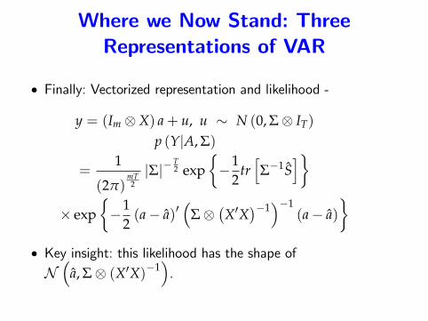
Where we Now Stand: ThreeRepresentations of VAR
• Finally: Vectorized representation and likelihood -
y = (Im ⊗X) a+ u, u ∼ N (0, Σ⊗ IT)
p (Y|A, Σ)
=1
(2π)mT2|Σ|−
T2 exp
{−1
2tr[Σ−1S
]}× exp
{−1
2(a− a)′
(Σ⊗
(X′X
)−1)−1
(a− a)}
• Key insight: this likelihood has the shape ofN(
a, Σ⊗ (X′X)−1).
Outline• Normal Likelihood, Illustrated with Simple AR(2)representation. (done!)— conditional versus unconditional likelihood.— maximum likelihood with level GDP data.— the Hurwicz bias.
• Three representations of a VAR. (done!)— Standard Representation— Matrix Representation— Vectorized Representation.
• Priors, posteriors and marginal likelihood— Dummy observations.— Conjugate Priors.
• Forecasting with BVARs— stochastic simulations, versus non-stochastic.— forecast probability intervals.
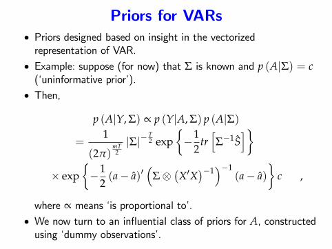
Priors for VARs• Priors designed based on insight in the vectorizedrepresentation of VAR.
• Example: suppose (for now) that Σ is known and p (A|Σ) = c(‘uninformative prior’).
• Then,
p (A|Y, Σ) ∝ p (Y|A, Σ) p (A|Σ)
=1
(2π)mT2|Σ|−
T2 exp
{−1
2tr[Σ−1S
]}× exp
{−1
2(a− a)′
(Σ⊗
(X′X
)−1)−1
(a− a)}
c ,
where ∝ means ‘is proportional to’.• We now turn to an influential class of priors for A, constructedusing ‘dummy observations’.
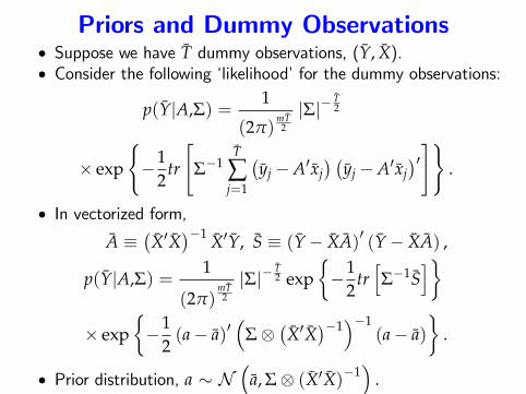
Priors and Dummy Observations• Suppose we have T dummy observations, (Y, X).• Consider the following ‘likelihood’for the dummy observations:
p(Y|A,Σ) =1
(2π)mT2
|Σ|−T2
× exp
{−1
2tr
[Σ−1
T
∑j=1
(yj −A′xj
) (yj −A′xj
)′]} .
• In vectorized form,
A ≡(X′X
)−1 X′Y, S ≡ (Y− XA)′ (Y− XA) ,
p(Y|A,Σ) =1
(2π)mT2
|Σ|−T2 exp
{−1
2tr[Σ−1S
]}× exp
{−1
2(a− a)′
(Σ⊗
(X′X
)−1)−1
(a− a)}
.
• Prior distribution, a ∼ N(
a, Σ⊗ (X′X)−1)
.
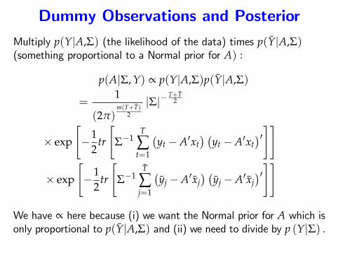
Dummy Observations and PosteriorMultiply p(Y|A,Σ) (the likelihood of the data) times p(Y|A,Σ)(something proportional to a Normal prior for A) :
p(A|Σ, Y) ∝ p(Y|A,Σ)p(Y|A,Σ)
=1
(2π)m(T+T)
2
|Σ|−T+T
2
× exp
[−1
2tr
[Σ−1
T
∑t=1
(yt −A′xt
) (yt −A′xt
)′]]
× exp
[−1
2tr
[Σ−1
T
∑j=1
(yj −A′xj
) (yj −A′xj
)′]]
We have ∝ here because (i) we want the Normal prior for A which isonly proportional to p(Y|A,Σ) and (ii) we need to divide by p (Y|Σ) .
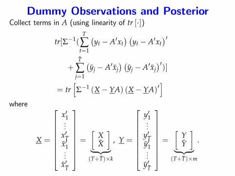
Dummy Observations and PosteriorCollect terms in A (using linearity of tr [·])
tr[Σ−1(T
∑t=1
(yt −A′xt
) (yt −A′xt
)′+
T
∑j=1
(yj −A′xj
) (yj −A′xj
)′)]
= tr[Σ−1 (X− YA) (X− YA)′
]where
X =
x′1...
x′Tx′1...
x′T
=
[XX
]︸ ︷︷ ︸(T+T)×k
, Y =
y′1...
y′Ty′1...
y′T
=
[YY
]︸ ︷︷ ︸(T+T)×m
.
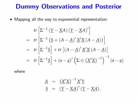
Dummy Observations and Posterior
• Mapping all the way to exponential representation:
tr[Σ−1 (Y−XA) (Y−XA)′
]= tr
[Σ−1 (S+ (A−A)′ X′X (A−A)
)]= tr
[Σ−1S
]+ tr
[(A−A)′ X′X (A−A)
]= tr
[Σ−1S
]+ (a− a)′
(Σ⊗
(X′X
)−1)−1
(a− a)
where
A =(X′X
)−1 X′Y
S = (Y−XA)′ (Y−XA) .
Dummy Observations and Posterior
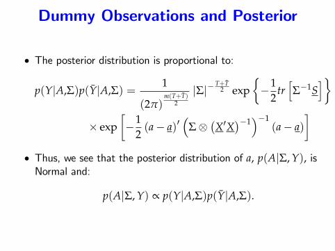
• The posterior distribution is proportional to:
p(Y|A,Σ)p(Y|A,Σ) =1
(2π)m(T+T)
2
|Σ|−T+T
2 exp{−1
2tr[Σ−1S
]}
× exp[−1
2(a− a)′
(Σ⊗
(X′X
)−1)−1
(a− a)]
• Thus, we see that the posterior distribution of a, p(A|Σ, Y), isNormal and:
p(A|Σ, Y) ∝ p(Y|A,Σ)p(Y|A,Σ).
Interpreting the Posterior
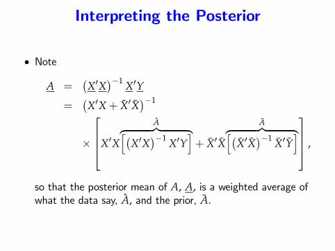
• Note
A =(X′X
)−1 X′Y
=(X′X+ X′X
)−1
×
X′X
A︷ ︸︸ ︷[(X′X
)−1 X′Y]+ X′X
A︷ ︸︸ ︷[(X′X
)−1 X′Y] ,
so that the posterior mean of A, A, is a weighted average ofwhat the data say, A, and the prior, A.
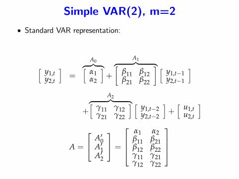
Simple VAR(2), m=2
• Standard VAR representation:
[ y1,ty2,t
]=
A0︷ ︸︸ ︷[α1α2
]+
A1︷ ︸︸ ︷[β11 β12β21 β22
] [ y1,t−1y2,t−1
]
+
A2︷ ︸︸ ︷[γ11 γ12γ21 γ22
] [ y1,t−2y2,t−2
]+[ u1,t
u2,t
]
A =
A′0A′1A′2
=
α1 α2β11 β21β12 β22γ11 γ21γ12 γ22
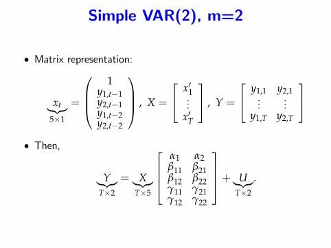
Simple VAR(2), m=2
• Matrix representation:
xt︸︷︷︸5×1
=
1
y1,t−1y2,t−1y1,t−2y2,t−2
, X =
x′1...
x′T
, Y =
y1,1 y2,1...
...y1,T y2,T
• Then,
Y︸︷︷︸T×2
= X︸︷︷︸T×5
α1 α2β11 β21β12 β22γ11 γ21γ12 γ22
+ U︸︷︷︸T×2
.
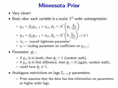
Minnesota Prior• Very clever!• Basic idea: each variable is a scalar 1st order autoregression:
— yi,t = βiiyi,t−1 + ui,t, βii ∼ N(
φi,Σii
λ21s2
i
)— yi,t = βijyj,t−1 + ui,t, βij ∼ N
(0, Σii
λ21s2
j
), j 6= i
— λ1 ∼ ‘overall tightness parameter’— si ∼ ‘scaling parameter on coeffi cient on yj,t−1’
• Parameter, φi :— if yi,t is in levels, then φi = 1 (random walk).— if yi,t is in first difference, then φi = 0 (again, random walk).— could have φi 6= 1.
• Analogous restrictions on lags 2, ..., p parameters.— Prior assumes that the data has less information on parametersat higher order lags.
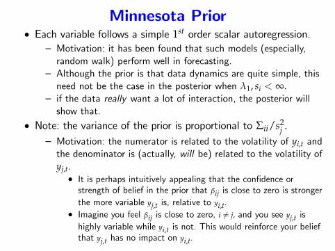
Minnesota Prior• Each variable follows a simple 1st order scalar autoregression.
— Motivation: it has been found that such models (especially,random walk) perform well in forecasting.
— Although the prior is that data dynamics are quite simple, thisneed not be the case in the posterior when λ1, si < ∞.
— if the data really want a lot of interaction, the posterior willshow that.
• Note: the variance of the prior is proportional to Σii/s2j .
— Motivation: the numerator is related to the volatility of yi,t andthe denominator is (actually, will be) related to the volatility ofyj,t.• It is perhaps intuitively appealing that the confidence orstrength of belief in the prior that βij is close to zero is strongerthe more variable yj,t is, relative to yi,t.
• Imagine you feel βij is close to zero, i 6= j, and you see yj,t ishighly variable while yi,t is not. This would reinforce your beliefthat yj,t has no impact on yi,t.
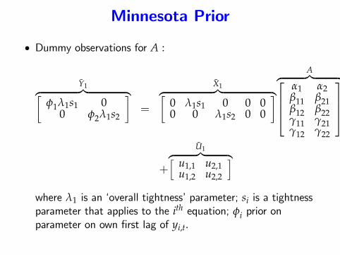
Minnesota Prior
• Dummy observations for A :
Y1︷ ︸︸ ︷[φ1λ1s1 0
0 φ2λ1s2
]=
X1︷ ︸︸ ︷[0 λ1s1 0 0 00 0 λ1s2 0 0
]A︷ ︸︸ ︷
α1 α2β11 β21β12 β22γ11 γ21γ12 γ22
+
U1︷ ︸︸ ︷[ u1,1 u2,1u1,2 u2,2
]where λ1 is an ‘overall tightness’parameter; si is a tightnessparameter that applies to the ith equation; φi prior onparameter on own first lag of yi,t.
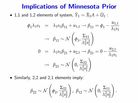
Implications of Minnesota Prior• 1,1 and 1,2 elements of system, Y1 = X1A+ U1 :
φ1λ1s1 = λ1s1β11 + u1,1 → β11 = φ1 −u1,1
λ1s1
→ β11 ∼ N(
φ1,Σ11
λ21s2
1
)0 = λ1s1β21 + u2,1 → β21 = 0− u2,1
λ1s1
→ β21 ∼ N(
0,Σ22
λ21s2
1
)• Similarly, 2,2 and 2,1 elements imply:
β22 ∼ N(
φ2,Σ22
λ21s2
2
), β12 ∼ N
(0,
Σ11
λ21s2
2
).
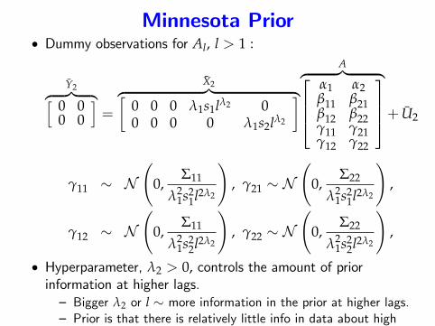
Minnesota Prior• Dummy observations for Al, l > 1 :
Y2︷ ︸︸ ︷[ 0 00 0
]=
X2︷ ︸︸ ︷[0 0 0 λ1s1lλ2 00 0 0 0 λ1s2lλ2
]A︷ ︸︸ ︷
α1 α2β11 β21β12 β22γ11 γ21γ12 γ22
+ U2
γ11 ∼ N(
0,Σ11
λ21s2
1l2λ2
), γ21 ∼ N
(0,
Σ22
λ21s2
1l2λ2
),
γ12 ∼ N(
0,Σ11
λ21s2
2l2λ2
), γ22 ∼ N
(0,
Σ22
λ21s2
2l2λ2
),
• Hyperparameter, λ2 > 0, controls the amount of priorinformation at higher lags.— Bigger λ2 or l ∼ more information in the prior at higher lags.— Prior is that there is relatively little info in data about highorder lags.
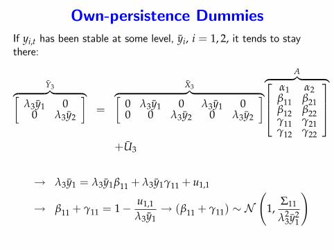
Own-persistence DummiesIf yi,t has been stable at some level, yi, i = 1, 2, it tends to staythere:
Y3︷ ︸︸ ︷[λ3y1 0
0 λ3y2
]=
X3︷ ︸︸ ︷[0 λ3y1 0 λ3y1 00 0 λ3y2 0 λ3y2
]A︷ ︸︸ ︷
α1 α2β11 β21β12 β22γ11 γ21γ12 γ22
+U3
→ λ3y1 = λ3y1β11 + λ3y1γ11 + u1,1
→ β11 + γ11 = 1− u1,1
λ3y1→ (β11 + γ11) ∼ N
(1,
Σ11
λ23y2
1
)
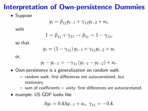
Interpretation of Own-persistence Dummies• Suppose
yt = β11yt−1 + γ11yt−2 + ut,
with1 = β11 + γ11 → β11 = 1− γ11,
so thatyt = (1− γ11) yt−1 + γ11yt−2 + ut
or,yt − yt−1 = −γ11 (yt−1 − yt−2) + ut.
• Own-persistence is a generalization on random walk.— random walk: first differences not autocorrelated, butstationary.
— sum of coeffi cients = unity: first differences are autocorrelated.
• example: US GDP looks like
∆yt = 0.4∆y−1 + ut, γ11 = −0.4.
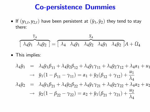
Co-persistence Dummies
• If (y1,t, y2,t) have been persistent at (y1, y2) they tend to staythere:
Y4︷ ︸︸ ︷[ λ4y1 λ4y2 ] =
X4︷ ︸︸ ︷[ λ4 λ4y1 λ4y2 λ4y1 λ4y2 ]A+ U4
• This implies:
λ4y1 = λ4y1β11 + λ4y2β12 + λ4y1γ11 + λ4y2γ12 + λ4α1 + u1
→ y1(1− β11 − γ11) = α1 + y2(β12 + γ12) +u1
λ4λ4y2 = λ4y1β21 + λ4y2β22 + λ4y1γ21 + λ4y2γ22 + λ4α2 + u2
→ y2(1− β22 − γ22) = α2 + y1(β21 + γ21) +u2
λ4
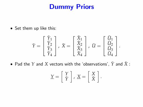
Dummy Priors
• Set them up like this:
Y =
Y1Y2Y3Y4
, X =
X1X2X3X4
, U =
U1U2U3U4
.
• Pad the Y and X vectors with the ‘observations’, Y and X :
Y =[
YY
], X =
[XX
].
Prior for Variance-Covariance Matrix
• Up to now, we’ve focused on the prior and posterior for theVAR parameters in A.
• We’ve supposed that the analyst ‘knows’the value of Σ.
• Next, we consider the more plausible case that the analyst alsodoes not know Σ.
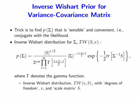
Inverse Wishart Prior forVariance-Covariance Matrix
• Trick is to find p (Σ) that is ‘sensible’and convenient, i.e.,conjugate with the likelihood.
• Inverse Wishart distribution for Σ, IW (S, ν) :
p (Σ) =|S|ν/2
2νmm
∏i=1
Γ[
ν+1−i2
] |Σ|− ν+m+12 exp
{−1
2tr[Σ−1S
]},
where Γ denotes the gamma function.
— Inverse Wishart distribution, IW (ν, S) , with ‘degrees offreedom’, ν, and ‘scale matrix’S.
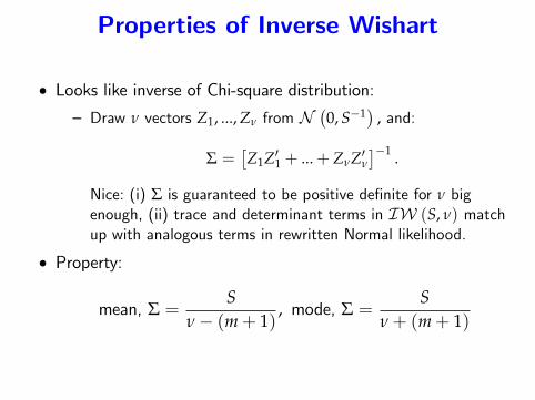
Properties of Inverse Wishart
• Looks like inverse of Chi-square distribution:— Draw ν vectors Z1, ..., Zν from N
(0, S−1) , and:
Σ =[Z1Z′1 + ...+ ZνZ′ν
]−1 .
Nice: (i) Σ is guaranteed to be positive definite for ν bigenough, (ii) trace and determinant terms in IW (S, ν) matchup with analogous terms in rewritten Normal likelihood.
• Property:
mean, Σ =S
ν− (m+ 1), mode, Σ =
Sν+ (m+ 1)
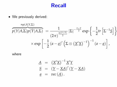
Recall
• We previously derived:
∝p(A|Y,Σ)︷ ︸︸ ︷p(Y|A,Σ)p(Y|A,Σ) =
1
(2π)m(T+T)
2
|Σ|−T+T
2 exp{−1
2tr[Σ−1S
]}
× exp[−1
2(a− a)′
(Σ⊗
(X′X
)−1)−1
(a− a)]
,
where
A =(X′X
)−1 X′Y
S = (Y−XA)′ (Y−XA)a = vec (A) .
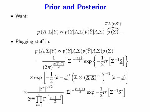
Prior and Posterior• Want:
p (A, Σ|Y) ∝ p(Y|A,Σ)p(Y|A,Σ)
IW(ν,S∗)︷ ︸︸ ︷p (Σ) .
• Plugging stuff in:
p (A, Σ|Y) ∝ p(Y|A,Σ)p(Y|A,Σ)p (Σ)
=1
(2π)m(T+T)
2
|Σ|−T+T
2 exp{−1
2tr[Σ−1S
]}
× exp[−1
2(a− a)′
(Σ⊗
(X′X
)−1)−1
(a− a)]
× |S∗|ν/2
2νmm
∏i=1
Γ[
ν+1−i2
] |Σ|− ν+m+12 exp−1
2tr[Σ−1S∗
]
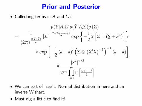
Prior and Posterior• Collecting terms in A and Σ :
p(Y|A,Σ)p(Y|A,Σ)p (Σ)
=1
(2π)m(T+T)
2
|Σ|−T+T+ν+m+1
2 exp{−1
2tr[Σ−1 (S+ S∗)
]}
× exp[−1
2(a− a)′
(Σ⊗
(X′X
)−1)−1
(a− a)]
× |S∗|ν/2
2νmm
∏i=1
Γ[
ν+1−i2
]• We can sort of ‘see’a Normal distribution in here and aninverse Wishart.
• Must dig a little to find it!
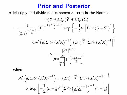
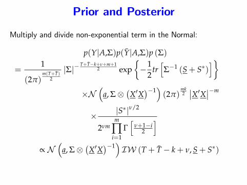
Prior and Posterior• Multiply and divide non-exponential term in the Normal:
p(Y|A,Σ)p(Y|A,Σ)p (Σ)
=1
(2π)m(T+T)
2
|Σ|−T+T+ν+m+1
2 exp{−1
2tr[Σ−1 (S+ S∗)
]}
×N(
a, Σ⊗(X′X
)−1)(2π)
mk2
∣∣∣Σ⊗ (X′X)−1∣∣∣ 1
2
× |S∗|ν/2
2νmm
∏i=1
Γ[
ν+1−i2
]where
N(
a, Σ⊗(X′X
)−1)= (2π)−
mk2
∣∣∣Σ⊗ (X′X)−1∣∣∣− 1
2
× exp[−1
2(a− a)′
(Σ⊗
(X′X
)−1)−1
(a− a)]
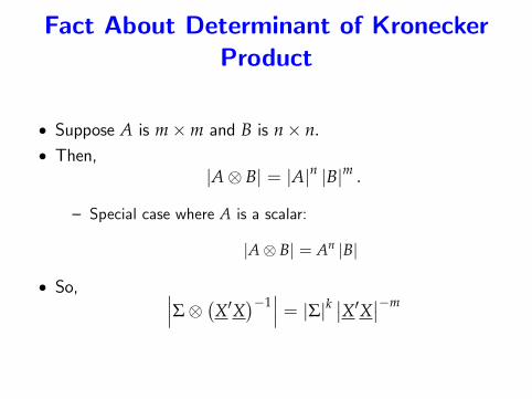
Fact About Determinant of KroneckerProduct
• Suppose A is m×m and B is n× n.• Then,
|A⊗ B| = |A|n |B|m .
— Special case where A is a scalar:
|A⊗ B| = An |B|
• So, ∣∣∣Σ⊗ (X′X)−1∣∣∣ = |Σ|k ∣∣X′X∣∣−m
Prior and Posterior
Multiply and divide non-exponential term in the Normal:
p(Y|A,Σ)p(Y|A,Σ)p (Σ)
=1
(2π)m(T+T)
2
|Σ|−T+T−k+ν+m+1
2 exp{−1
2tr[Σ−1 (S+ S∗)
]}×N
(a, Σ⊗
(X′X
)−1)(2π)
mk2∣∣X′X∣∣−m
× |S∗|ν/2
2νmm
∏i=1
Γ[
ν+1−i2
]∝ N
(a, Σ⊗
(X′X
)−1)IW (T+ T− k+ ν, S+ S∗)
Prior and Posterior
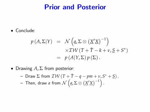
• Conclude:
p (A, Σ|Y) = N(
a, Σ⊗(X′X
)−1)
×IW (T+ T− k+ ν, S+ S∗)= p (A|Y, Σ) p (Σ) .
• Drawing A, Σ from posterior:
— Draw Σ from IW (T+ T− q− pm+ ν, S∗ + S) .— Then, draw a from N
(a, Σ⊗
(X′X
)−1)
.
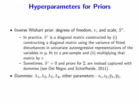
Hyperparameters for Priors
• Inverse Wishart prior: degrees of freedom, ν, and scale, S∗.— In practice, S∗ is a diagonal matrix constructed by (i)constructing a diagonal matrix using the variance of fitteddisturbances in univariate autoregressive representations of thevariables in yt fit to a pre-sample and (ii) multiplying thatmatrix by ν.
— Sometimes, S∗ = 0 and priors for Σ are instead captured withdummies (see Del Negro and Schorfheide, 2011).
• Dummies: λ1, λ2, λ3, λ4, other parameters - s1, s2, y1, y2.
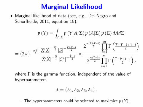
Marginal Likelihood• Marginal likelihood of data (see, e.g., Del Negro andSchorfheide, 2011, equation 15):
p (Y) =∫
A,Σp (Y|A, Σ) p (A|Σ) p (Σ) dAdΣ
= (2π)−mT2
∣∣X′X∣∣−m2 |S|−
T+T−k2
|X′X|−m2 |S∗|−
T−k2
×2
m(T+T−k)2
m
∏i=1
Γ(
T+T−k+1−i2
)2
m(T−k)2
m
∏i=1
Γ(
T−k+1−i2
),
where Γ is the gamma function, independent of the value ofhyperparameters,
λ = (λ1, λ2, λ3, λ4) .
— The hyperparameters could be selected to maximize p (Y) .
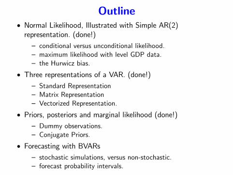
Outline• Normal Likelihood, Illustrated with Simple AR(2)representation. (done!)— conditional versus unconditional likelihood.— maximum likelihood with level GDP data.— the Hurwicz bias.
• Three representations of a VAR. (done!)— Standard Representation— Matrix Representation— Vectorized Representation.
• Priors, posteriors and marginal likelihood (done!)— Dummy observations.— Conjugate Priors.
• Forecasting with BVARs— stochastic simulations, versus non-stochastic.— forecast probability intervals.
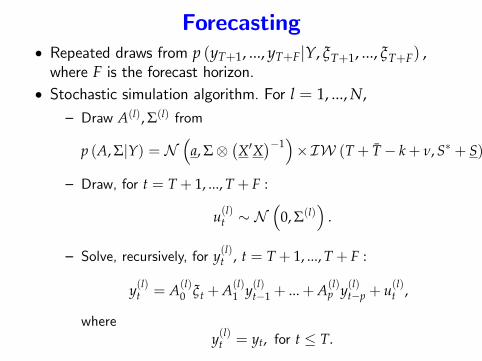
Forecasting• Repeated draws from p (yT+1, ..., yT+F|Y, ξT+1, ..., ξT+F) ,where F is the forecast horizon.
• Stochastic simulation algorithm. For l = 1, ..., N,— Draw A(l), Σ(l) from
p (A, Σ|Y) = N(
a, Σ⊗(X′X
)−1)×IW (T+ T− k+ ν, S∗ + S) .
— Draw, for t = T+ 1, ..., T+ F :
u(l)t ∼ N(
0, Σ(l))
.
— Solve, recursively, for y(l)t , t = T+ 1, ..., T+ F :
y(l)t = A(l)0 ξt +A(l)1 y(l)t−1 + ...+A(l)p y(l)t−p + u(l)t ,
wherey(l)t = yt, for t ≤ T.
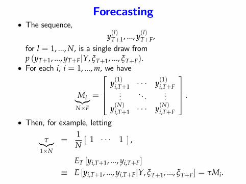
Forecasting• The sequence,
y(l)T+1, ..., y(l)T+F,for l = 1, ..., N, is a single draw fromp (yT+1, ..., yT+F|Y, ξT+1, ..., ξT+F).
• For each i, i = 1, ..., m, we have
Mi︸︷︷︸N×F
=
y(1)i,T+1 · · · y(1)i,T+F...
. . ....
y(N)i,T+1 · · · y(N)i,T+F
.
• Then, for example, letting
τ︸︷︷︸1×N
=1N[ 1 · · · 1 ] ,
ET [yi,T+1, ..., yi,T+F]
≡ E [yi,T+1, ..., yi,T+F|Y, ξT+1, ..., ξT+F] = τMi.
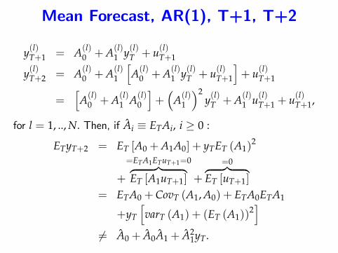
Mean Forecast, AR(1), T+1, T+2
y(l)T+1 = A(l)0 +A(l)1 y(l)T + u(l)T+1
y(l)T+2 = A(l)0 +A(l)1
[A(l)0 +A(l)1 y(l)T + u(l)T+1
]+ u(l)T+1
=[A(l)0 +A(l)1 A(l)0
]+(
A(l)1
)2y(l)T +A(l)1 u(l)T+1 + u(l)T+1,
for l = 1, .., N. Then, if Ai ≡ ETAi, i ≥ 0 :
ETyT+2 = ET [A0 +A1A0] + yTET (A1)2
+
=ETA1ETuT+1=0︷ ︸︸ ︷ET [A1uT+1] +
=0︷ ︸︸ ︷ET [uT+1]
= ETA0 + CovT (A1, A0) + ETA0ETA1
+yT
[varT (A1) + (ET (A1))
2]
6= A0 + A0A1 + A21yT.
Message of Previous Slide
• To obtain mathematically correct mean forecast, ETyT+i,i = 1, ..., F,
— must do stochastic simulations of future.— simple non-stochastic simulations not enough:
y(l)t = A0ξt + A1yt−1 + ...+ Apyt−p,
setting ETuT+i = 0 for i = 1, ..., F.
• Problem with non-stochastic simulation procedure isquantitatively large if there is a lot of uncertainty at T about Aand Σ (e.g., posterior second moments of A are large).
— Whether it is worth the extra time to do stochastic simulationmust be assessed on case by case basis.
Forecast Probability Interval
• After stochastic simulation, we have:
Mi︸︷︷︸N×F
=
y(1)i,T+1 · · · y(1)i,T+F...
. . ....
y(N)i,T+1 · · · y(N)i,T+F
,
for i = 1, ..., m.• To obtain the date T conditional distribution of yi,T+j displayhistogram of jth column of Mi.
• 90% probability interval for yi,T+j obtained by:
— sorting contents of ith column of Mi from smallest to largest— reporting 50th and 950th elements (say, N = 1, 000).