Embed Size (px)
Citation preview

BeamPROP 8.0 User Guide
RSoft Design Group, Inc. 400 Executive Blvd. • Suite 100 Ossining, NY 10562 Phone: 1•914•923•2164 Fax: 1•914•923•2169 [email protected] www.rsoftdesign.com Copyright © 1993 - 2007 All Rights Reserved.

BeamPROP 8.0 User Guide Contents • iii
Contents
Preface 1 What’s new in version 8.0 .........................................................................................................3 What was new in version 7.0 .....................................................................................................3 Notices .......................................................................................................................................3
Limited Warranty ........................................................................................................3 Copyright Notice .........................................................................................................3 RSoft Design Group™ Trademarks ............................................................................4 Acknowledgments .......................................................................................................4
System Requirements ................................................................................................................4 How to read this manual ............................................................................................................5
What should I read and when? ....................................................................................5 Where can I find the documentation for…..................................................................5
Conventions ...............................................................................................................................6 Physics Conventions.................................................................................................... 6
Chapter 1: Installation 9 1.A. Main Program Installation .................................................................................................9
1.A.1. Installation Overview .......................................................................................9 1.A.2. Backing up the Examples ................................................................................. 9
1.B. Testing the BeamPROP installation ................................................................................10 1.C. What Next? ......................................................................................................................12
README File...........................................................................................................12 Technical Support & Software Upgrades ..................................................................12
Chapter 2: Background 15 2.A. Background......................................................................................................................15 2.B. Review of the Beam Propagation Method (BPM) ...........................................................16
2.B.1. Scalar, Paraxial BPM......................................................................................16 2.B.2. Numerical Solution and Boundary Conditions ...............................................18 2.B.3. Including Polarization - Vector BPM .............................................................19 2.B.4. Removing Paraxiality – Wide-Angle BPM.....................................................20 2.B.5. Handling Reflections – Bi-directional BPM...................................................21 2.B.6. Additional BPM Techniques...........................................................................21 2.B.7. Mode Solving via BPM ..................................................................................21 2.B.8. References.......................................................................................................23
2.C. General guidelines for Using BPM .................................................................................. 25 2.C.1. Overview......................................................................................................... 26 2.C.2. General Philosophy for Choosing Parameters ................................................ 26
Chapter 3: A First Tour of BeamPROP 29 3.A. Component Programs and Files .......................................................................................29
3.A.1. Component Executables .................................................................................29 3.A.2. Example Files .................................................................................................30
iv • Contents BeamPROP 8.0 User Guide
3.B. Program Operation ...........................................................................................................30 3.B.1. GUI Program Operation..................................................................................31 3.B.2. CLI Operation .................................................................................................33
Chapter 4: Using BeamPROP 35 4.A. Spatial Grid ......................................................................................................................35 4.B. The Launch Condition......................................................................................................36
4.B.1. Creating a Launch Field..................................................................................37 4.B.2. Polarization Manipulation...............................................................................42 4.B.3. Launching Multiple Fields..............................................................................42
4.C. Advanced & Bidirectional BPM Options.........................................................................42 4.D. Display and Output Options.............................................................................................42
4.D.1. Display Options .............................................................................................. 43 4.D.2. Output Options ...............................................................................................46
Chapter 5: Monitoring and Analysis of Simulation Results 49 5.A. Defining a Pathway..........................................................................................................49 5.B. Creating a Monitor ...........................................................................................................49 5.C. Assigning a Pathway to the Monitor ................................................................................50 5.D. Choosing a Monitor Type ................................................................................................50
Note for Phase Monitors............................................................................................52 5.E. Monitor Options ...............................................................................................................52
Chapter 6: Mode Solving 55 6.A. Background......................................................................................................................55 6.B. Mode Solving Overview ..................................................................................................55
Step 1: Create the index structure in the RSoft CAD tool. .......................................55 Step 2: Choose the appropriate mode solver and related options. ............................55 Step 3: Choose Launch Field....................................................................................56 Step 3: Choose the mode calculation parameters ......................................................57 Step 5: Perform the mode calculation.......................................................................57
6.C. Using the Iterative Method...............................................................................................58 6.C.1. Computing Modes...........................................................................................58 6.C.2. Additional Notes .............................................................................................58
6.D. Using the Correlation Method..........................................................................................59 6.D.1. Computing only the Mode Spectrum..............................................................59 6.D.2. Computing the Mode Profiles and Propagation Constants .............................59 6.D.3. Additional Notes............................................................................................. 60
6.E. Additional Comments.......................................................................................................61 6.E.1. Finding Asymmetric Higher Order Modes with the Iterative Method ............61 6.E.2. Calculating Modes from the Command Line .................................................. 61 6.E.3. Saving the Magnetic Field ..............................................................................61 6.E.4. Parameter Scans ..............................................................................................61 6.E.5. Setting the Mode Calculation Length..............................................................62
6.F. References ........................................................................................................................62
Chapter 7: Advanced Simulation Features 63 7.A. Incorporating Polarization Effects (Vector BPM) ........................................................... 63
7.A.1. Vector Simulation Options .............................................................................63 7.A.2. 2D Vector BPM..............................................................................................64 7.A.3. 3D Vector BPM..............................................................................................65 7.A.4. Manipulating the Polarization of the Launch Field ........................................65 7.A.5. Vector BPM and the Effective Index Calculation Option ..............................68

BeamPROP 8.0 User Guide Contents • v
7.B. Advanced Numerical Options ..........................................................................................68 7.B.1. BPM Options .................................................................................................. 69 7.B.2. Boundary Conditions ......................................................................................72
7.C. Bidirectional Calculation Options.................................................................................... 73 7.C.1. Background..................................................................................................... 73 7.C.2. Enabling a Bidirectional BPM Simulation......................................................74 7.C.3. Bidirectional Parameters................................................................................. 74
7.D. Defining Simulation Regions...........................................................................................76 7.D.1. Why Use a Simulation Region?...................................................................... 76 7.D.2. Defining a Simulation Region ........................................................................76
7.E. Anisotropy, Non-Linearity, and Dispersion .....................................................................77 7.F. Calculation Electrodes/Heater Effects ..............................................................................77
7.F.1. Defining Electro-Optic Material...................................................................... 78 7.F.2. Creating Electrodes/Heaters in the CAD.........................................................79 7.F.3. Using the Electrode/Heater Utility ..................................................................80 7.F.4. Additional Notes ............................................................................................. 80
7.G. Radial BPM......................................................................................................................81 7.G.1 Using Radial BPM...........................................................................................81 7.G.2. Displaying 3D Results ....................................................................................81
7.H. Effective Index Calculations............................................................................................82
Chapter 8: Basic Tutorials 83 Basic Tutorial 1: Basic 2D Simulation ...................................................................................83
CAD Window Basics ................................................................................................83 Creating a New Circuit ..............................................................................................85 Creating Variables via the Symbol Table..................................................................87 Adding the Waveguide ..............................................................................................88 Choosing the Excitation ............................................................................................90 Adding a Pathway .....................................................................................................92 Adding a Monitor ......................................................................................................92 Performing the Simulation ........................................................................................93 The Simulation Window............................................................................................94 Accessing Saved Data ...............................................................................................95 Areas for Further Exploration: ..................................................................................97
Basic Tutorial 2: Basic 3D Simulation ...................................................................................99 3D Specific CAD Options .........................................................................................99 Creating Variables ................................................................................................... 100 Adding the Fiber Segment....................................................................................... 101 Viewing the Structure in 3D.................................................................................... 101 Checking the Index Profile ...................................................................................... 102 Choosing the Excitation Field ................................................................................. 104 Adding a Pathway and Monitor............................................................................... 104 Performing the Simulation ......................................................................................105 Accessing Saved Data ............................................................................................. 107 Areas for Further Exploration..................................................................................107
Chapter 9: Tutorial Examples 109 Tutorial 1 - Using the Multilayer Structure Type .................................................................. 109
The Multilayer Geometry ........................................................................................109 Device Layout ......................................................................................................... 109 Analysis Setup.........................................................................................................116 Performing the Simulation ......................................................................................117 Performing A Mode Calculation .............................................................................120 Further Exploration .................................................................................................122
vi • Contents BeamPROP 8.0 User Guide
Tutorial 2 - Simulating S-Bends ............................................................................................123 Device Layout via Actual Bends .............................................................................123 Device Layout via Simulated Bend Feature ............................................................128 Simulation (Offset Optimization)............................................................................ 131 Performing the Simulation ......................................................................................138 Using the Actual S-Bend ......................................................................................... 138
Tutorial 3 - Multimode Interference or MMI Devices........................................................... 141 Device Layout ......................................................................................................... 141 Analysis Setup.........................................................................................................145 Performing the Simulation ......................................................................................150
Tutorial 4 - Using User-Defined Index Profiles..................................................................... 153 Device Layout ......................................................................................................... 153 Computing a Mode..................................................................................................156
Tutorial 5 - Using Multiple Launch Fields ............................................................................159 Device Layout ......................................................................................................... 159 Drawing the Waveguides ........................................................................................ 159 Performing the Simulation ......................................................................................164
Tutorial 6 - Leaky Modes in a Hollow Fiber .........................................................................169 Device Layout ......................................................................................................... 169 Calculating the Mode .............................................................................................. 174
Tutorial 7 - Using Wide-Angle BPM.....................................................................................179 Device Layout ......................................................................................................... 179 Analysis Setup.........................................................................................................181 Experimenting with Wide Angle Propagation.........................................................183 Final Remarks.......................................................................................................... 187
Tutorial 8 - Using Bidirectional BPM for Modeling Gratings............................................... 189 Device Layout ......................................................................................................... 189 Analysis Setup.........................................................................................................194 Simulation ............................................................................................................... 195 Further Exploration .................................................................................................199
Tutorial 9 - Using the Electrode Feature................................................................................201 Device Layout ......................................................................................................... 201 Electrode Layer and Electrode Setup and Simulation ............................................. 207 Analysis Setup.........................................................................................................212 Simulation ............................................................................................................... 213
Tutorial 10 - Using The WDM Router (AWG) Utility ......................................................... 217 Tutorial 11: Using The Simulation Region Feature.............................................................. 219
Device Layout ......................................................................................................... 219 Analysis Setup.........................................................................................................222 Simulation ............................................................................................................... 224 Using Simulation Region Feature............................................................................ 228 Summary ................................................................................................................. 232
References ............................................................................................................................. 233
Chapter 10: Mode Solving Tutorials 235 Mode Tutorial 1: Using the Iterative Method ....................................................................... 235
Modes of a Simple 2D Slab..................................................................................... 235 Modes of a Simple 3D Buried Channel...................................................................238 Performing Convergence Studies ............................................................................239 Areas for Further Exploration..................................................................................243
Mode Tutorial 2: Using the Correlation Method .................................................................. 245 Modes of a Simple 2D Slab..................................................................................... 245 Modes of a Simple Fiber Structure..........................................................................248 Areas for Further Exploration..................................................................................250
Mode Tutorial 3: Computing the Mode Cutoff..................................................................... 251
BeamPROP 8.0 User Guide Contents • vii
Creating the Structure.............................................................................................. 251 Setting Simulation Parameters................................................................................. 251 Parameter Scan for Mode Cutoff.............................................................................252 Areas for Further Exploration..................................................................................253
Mode Tutorial 4: Dispersion in Single Mode Silica Fibers .................................................. 255 Creating the Structure.............................................................................................. 255 Computing Dispersion with MOST ......................................................................... 256 Areas for Further Exploration..................................................................................259
Mode Tutorial 5: Index Guided Photonic Crystal Fibers...................................................... 261 Creating the PCF Structure...................................................................................... 261 Computing the PCF Mode.......................................................................................262 Exploring the Single-Mode Condition.....................................................................263 Areas for Further Exploration..................................................................................266
Mode Tutorial 6: Leaky Modes of a Rib Waveguide ...........................................................267 Creating the Structure.............................................................................................. 267 Computing the Mode............................................................................................... 269 Areas for Further Exploration..................................................................................271
Mode Tutorial 7: Modes with a Non-Uniform Grid ............................................................. 273 Structure Overview.................................................................................................. 273 Advantages of Using a Non-Uniform Grid for this Structure.................................. 273 Creating a Non-Uniform Grid ................................................................................. 274 Modes with a Non-Uniform Grid ............................................................................ 275 Modes with a Uniform Grid .................................................................................... 276 Comparing the Results ............................................................................................ 276 Αρεασ φορ Φυρτηερ Εξπλορατιον ..................................................................... 277
Appendix A: Tips and Traps in BeamPROP 279 Common BeamPROP mistakes ............................................................................................. 279 Some Good BeamPROP habits to learn................................................................................. 279
Appendix B: BeamPROP File Formats 281 Index (*.ind) File Format....................................................................................................... 281 Graph File Format.................................................................................................................. 281 Standard RSoft File Format ................................................................................................... 282
Supported Output Types.......................................................................................... 283 Example Files .......................................................................................................... 284
Monitor File Format .............................................................................................................. 287 Correlation File Format ......................................................................................................... 287 Mode Spectrum File Format .................................................................................................. 287 Mode Results (Effective Index) File Format .........................................................................288 *.mds File Format.................................................................................................................. 288 Mode Field File Format ......................................................................................................... 289 Refractive Index and Loss Profile File Formats .................................................................... 289 Electrode/Heater Formats ......................................................................................................289
Appendix C: Symbol Table Variables 291 BPM Simulation Parameters.................................................................................................. 291 Advanced Grid Parameters ....................................................................................................292 Advanced Numerical Parameters........................................................................................... 292 Bi-Directional Parameters...................................................................................................... 293 Display Options ..................................................................................................................... 293 Output Options ...................................................................................................................... 294 Launch Parameters................................................................................................................. 294
viii • Contents BeamPROP 8.0 User Guide
Mode Solving ........................................................................................................................ 295 Mode Calculation Options....................................................................................... 295 Advanced Mode Solving Features........................................................................... 295
Boundary Conditions ............................................................................................................. 295 Additional Features................................................................................................................ 296 Compute Index Profile........................................................................................................... 296
Appendix D: BeamPROP Release Notes 297 Changes from Version 7.0 to Version 7.1.............................................................................. 297
New Capabilities and Improvements to the Program .............................................. 297 Significant Changes in Program Behavior .............................................................. 297
Changes from Version 6.0 to Version 7.0.............................................................................. 297 New Capabilities and Improvements to the Program .............................................. 298 Significant Changes in Program Behavior .............................................................. 298
Changes from Version 5.1 to Version 6.0.............................................................................. 298 New Capabilities and Improvements to the Program .............................................. 298 Significant Changes in Program Behavior .............................................................. 299
Changes from Version 5.0 to Version 5.1.............................................................................. 299 New Capabilities and Improvements to the Program .............................................. 300 Significant Changes in Program Behavior .............................................................. 300
Changes from Version 4.0 to Version 5.0.............................................................................. 301 New Capabilities and Improvements to the Program .............................................. 301 Significant Changes in Program Behavior .............................................................. 303
Changes from Version 3.0 to Version 4.0.............................................................................. 304 New Capabilities and Improvements to the Program .............................................. 304 Significant Changes in Program Behavior .............................................................. 307
Changes from Version 2.1 to Version 3.0.............................................................................. 308 New Capabilities and Improvements to the Program .............................................. 308 Significant Changes in Program Behavior .............................................................. 309
Changes from Version 2.0 to Version 2.1.............................................................................. 309 New Capabilities and Improvements to the Program .............................................. 309 Significant Changes in Program Behavior .............................................................. 310
Changes from Version 1.1 to Version 2.0.............................................................................. 310 New Capabilities and Improvements to the Program .............................................. 310 Significant Changes in Program Behavior .............................................................. 310
Changes from Version 1.0 to Version 1.1.............................................................................. 311 New Capabilities and Improvements to the Program .............................................. 311 Significant Changes in Program Behavior .............................................................. 312
Index 313

BeamPROP 8.0 User Guide Preface • 1
Preface
The BeamPROP simulation engine is a part of the RSoft Photonics Suite, and is based on advanced finite-difference beam propagation (BPM) techniques. It is fully integrated into the RSoft CAD environment which allows the user to define the material properties and structural geometry of a device. It is ideal for the design and modeling of photonic devices and photonic integrated circuits. The benefit of good design and modeling tools is well known in the electronics industry, where both device and circuit simulation programs, such as PICSES and SPICE have been instrumental in advancing the availability and use of integrated electronic circuits. BeamPROP brings this important capability to the photonics area, and can be an extremely useful tool for research and development groups in both university and industrial environments.
To use BeamPROP effectively, it is critical to have a working knowledge of the RSoft CAD interface. The CAD tool is described in full in the RSoft CAD manual, which is included in the BeamPROP package. The reader is strongly encouraged to study the CAD manual before reading beyond Chapter 3 of this manual.
As a member of the RSoft Photonics Suite, BeamPROP is designed to work with RSoft’s other passive device simulation modules FullWAVE, BandSOLVE, GratingMOD, DiffractMOD, and FemSIM. This modular approach to the design and simulation of photonic devices is one of RSoft’s Photonic Suite’s greatest strengths. Each program in the suite is designed to “play nice” with the other programs, creating an environment in which data can be shared between the modules. Virtually all the input and output files are in a simple ASCII text format, which allows even greater user control over program operation as well as third-party programs to be integrated into the suite.
While the RSoft Photonics Suite is designed to be used via the GUI (Graphical User Interface), command line operation is also possible. This, coupled with the modularity of the Suite, allows for complex scripting capability. The Suite is not limited to a single scripting language, but rather uses the native scripting language of your operating system. For example, Windows users can use DOS batch files, while Unix users can use bash scripts. Additionally, users familiar with languages such as Perl, Python, C, or C++ can create custom scripts in these languages. The RSoft Photonics Suite provides the best of both worlds: it allows for simulations to be performed via the GUI, and for complicated custom simulations to be performed via a script. New and advanced users alike are able to realize the full power of the Suite.

2 • Preface BeamPROP 8.0 User Guide

BeamPROP 8.0 User Guide Preface • 3
What’s new in version 8.0 Version 8.0 of BeamPROP contains a large number of new features. These are the highlights:
• Updated CAD Interface
The CAD interface has been updated to include a 3D editing capability as well as other improvements. See the CAD manual for more details.
What was new in version 7.0 Version 7.0 of BeamPROP contains a large number of new features. These are the highlights:
• New Non-Uniform Grid Options
The CAD contains a major new feature for non-uniform grid simulation. See Chapter 9 in the CAD manual.
• Improved Grid Generation
The index generation algorithms used by the CAD to compute the refractive index of a structure have been improved resulting in increased simulation accuracy. Grid points that lie at material interfaces are computed accurately, structure types can be freely mixed, and support for polygons has been improved.
• New Material Editor
The material editor is a completely new way to specify material parameters. Once defined, the material can be assigned to individual segments in a design. The user can define both linear and non-linear relative permittivity epsilon as a function of frequency. See Chapter 8 in the CAD manual for details.
Of course, a number of minor improvements have been added.
For full details on all changes, please consult the complete changelog for the RSoft CAD which is available in the README file, readmebp.txt, in the README subdirectory in the main installation directory.
Notices This section has a list of legal and other miscellaneous information pertaining to the software.
Limited Warranty RSoft Design Group, Inc. warrants that under normal use, the physical media (diskette and documentation) will be free of material defects for a period of thirty days from the date of purchase. Upon written notice, RSoft Design Group, Inc. will replace any defective media. No other warranty of any sort, either expressed or implied, is provided with this software. No liability for damage to equipment or data, or any other liability, is assumed by RSoft Design Group, Inc.
Copyright Notice Copyright © 1993-2007 RSoft Design Group, Inc. All Rights Reserved.
Copyright is claimed for both this manual and the software described in it.

4 • Preface BeamPROP 8.0 User Guide
RSoft Design Group™ Trademarks RSoft Design Group, RSoft Inc., RSoft, The RSoft CAD Environment, BeamPROP, FullWAVE, BandSOLVE, GratingMOD, DiffractMOD, FemSIM, LaserMOD, OptSIM, LinkSIM, EDFA for Vendors, ModeSYS, Artifex, MetroWAND, SWAT, WinPLOT, and RPlot are trademarks of RSoft Design Group, Inc.
Acknowledgments IBM is a registered trademark and IBM PC, PS/2, and OS/2 are trademarks of International Business Machines Corporation. Intel is a trademark of Intel Corporation. Microsoft and MS- DOS are registered trademarks and Windows is a trademark of Microsoft Corporation. UNIX and Motif are registered trademarks and X Windows is a trademark of The Open Group. Linux is a registered trademark of Linus Torvolds. Xfree86 is a registered trademark of the The Xfree86 Project. All other product names referred to in this document are trademarks or registered trademarks of their respective manufacturers.
System Requirements The RSoft Passive Device Suite will run on an IBM compatible personal computer with an Intel Pentium III or higher processor (or AMD equivalent), 256 MB RAM or higher depending on the application, and 250 MB of hard-disk space. Versions for 32-bit and 64-bit Windows and Linux are available. The Windows versions require Windows 2000/XP/Vista. Linux versions have been tested on the standard Red Hat configuration using X Windows or Xfree86 and Motif.

BeamPROP 8.0 User Guide Preface • 5
How to read this manual The following are some guidelines on the contents of this manual and the conventions used within it.
What should I read and when? You should begin by reading Chapters 1 and 2 to ensure that the installation was successful and to gain some initial impressions of its capabilities. Chapter 3 gives an overview of the package and program operation. Before proceeding to Chapter 4 and further, it is recommended that you gain a working familiarity with the RSoft CAD tool. The CAD manual and exercises should be studied until the user is reasonably familiar with the CAD interface, and is comfortable laying out simple photonic structures in the CAD tool.
Several Appendices at the end of this manual contain additional information.
Where can I find the documentation for… The documentation for the RSoft Photonics Suite is divided into several manuals. The manuals are structured using a simple rule:
Anything defining geometry and/or material parameters is in the CAD manual. Anything else is in an appropriate simulation manual.
Using this rule, almost any topic can be found. As with any rule, there are a few exceptions. The major exceptions are:
• Installation
The installation procedure for RSoft software, including the CAD and all simulation modules, is covered in the separate document entitled “RSoft Installation Guide”. Specific installation instructions for BeamPROP can be found in Chapter 1 of the this document.
• Using a Non-Uniform Grid
The creation of a non-uniform grid is covered in Chapter 9 of the CAD manual.
• Material Editor
The definition of advanced materials via the Material Editor is covered in Chapter 8 of the CAD manual.
• Parameter Scanning/Scripting/Batch Operation
These topics are very similar, and are shared by all the simulation modules. They are discussed in Chapter 10 of the CAD manual.
• Computing the Index Profile
Computing the index profile is discussed in the CAD manual.
• Pathways
Pathways define the location and geometry of launch, or initial fields in BeamPROP and FullWAVE. They are also used to define the locations of BeamPROP monitors. They are documented in the CAD manual.
• Command Line Utilities
The RSoft Photonics CAD Suite ships with several command line utilities which perform a variety of tasks. These utilities are documented in an Appendix in the CAD manual..
• RSoft Expressions

6 • Preface BeamPROP 8.0 User Guide
Virtually any numeric field in any RSoft product can accept an analytical expression involving pre-defined and user-defined variables. The form of these expressions, including valid arithmetic operators and functions can be found in an Appendix in the CAD manual.
Anytime this rule is violated, a note will direct the reader to the proper section in the proper manual. The location of these manuals is described in the next section.
Where are these manuals located? While each of the simulation modules are licensed separately, the documentation for each module is placed on your computer during installation.
Online versions can be accessed through the RSoft CAD via the Help menu item, or the two help buttons on the right of the top toolbar. The actual files can be found in the subdirectory help in the installation directory. Additionally, PDF versions can be found in the subdirectory docs. These files require the Adobe Acrobat Reader, which can be obtained from Adobe (www.acrobat.com) at no charge.
Conventions This section describes various conventions concerning the physics, the manual, and the product names.
Physics Conventions As with any branch of science, there are a number of concepts in the study of photonic devices for which there exist several different definitions exist in the literature. There are the conventions adopted in this tool:
Polarization Polarization is defined, in terms of the E field, as follows in BeamPROP: Simulation Type TE TM
2D (in XZ plane) Ey Ex
3D Ex Ey
Additional details on the RSoft Polarization convention can be found in the CAD manual Appendices
Units • All units of length are measured in microns [µm].
• All angular units are in degrees.
• The units of imaginary refractive index are defined as:
4imagn γλπ
=
where λ is the wavelength and γ is the usual exponential loss coefficient defined such that the power
decays as ze γ− , and is given in units of µm.
Manual Conventions A number of typeface and layout conventions are followed in this manual.
• Actions to be performed in the graphical interfaces are usually indented in bulleted or numbered lists.

BeamPROP 8.0 User Guide Preface • 7
• The names of fields and controls in the GUI dialogs are written in boldface Courier
• The values of pull-down menus and radio button controls are written in Roman italics.
• Symbol table variables and formulas, and expressions to be typed into the GUI edit fields are written in Courier.
• In referring to example CAD files, the installation directory for the CAD tool is specified as <rsoft_dir>, and should be replaced with the correct value for your installation. On Windows machines this is typically c:\Rsoft.
Product Name Conventions The executable files for the various RSoft products have different names under Windows and Unix/Linux. In the manual, we normally use the Windows names. The following table shows the corresponding names that should be used under Linux:
Product Windows Name Linux Name
RSoft CAD tool bcadw32.exe xbcad
BeamPROP simulation tool bsimw32.exe xbeam
FullWAVE simulation tool fullwave.exe xfullwave
WinPLOT graphing tool winplot.exe xplot
MOST rsmost.exe xrsmost


BeamPROP 8.0 User Guide Chapter 1: Installation • 9
Chapter 1: Installation
This chapter explains the installation procedure for BeamPROP, and provides a quick example to test the installation.
1.A. Main Program Installation This section details the installation of BeamPROP.
1.A.1. Installation Overview
Existing RSoft users Provided you have purchased and installed a license for RSoft software such as FullWAVE, BandSOLVE, or GratingMOD, there is a minimal amount of additional installation required to use BeamPROP. This is because BeamPROP shares the same CAD interface with these products.
You will have to replace the license file you are currently using with the one RSoft has sent you with your purchase. If your copy of RSoft software does not use a license file, please see the section under First-time RSoft users below for instructions on installing the license file. Note that if the existing version of BeamPROP, FullWAVE, BandSOLVE, GratingMOD, DiffractMOD, and/or FemSIM that you have is not the current version, you may also have to upgrade to the new version.
First-time RSoft users If you have not previously installed RSoft software, you should turn to the RSoft CAD manual and follow the installation instructions found there.
1.A.2. Backing up the Examples BeamPROP comes with a large set of examples and tutorial files which we use extensively in this manual. Since it is easy to accidentally overwrite these files in the course of experimenting with the tool, we recommend copying the entire examples directory in the BeamPROP install directory to another location, perhaps a subdirectory of your own home directory. Then you can perform the exercises and tutorials and retrieve the original versions when necessary. We suggest you do this now if you have not already.
• Windows:
Copy the directory <rsoft_dir>\examples to a suitable location.
• Linux:
Copy the directory /usr/local/rsoft/examples to a suitable subdirectory of your home directory.
10 • Chapter 1: Installation BeamPROP 8.0 User Guide
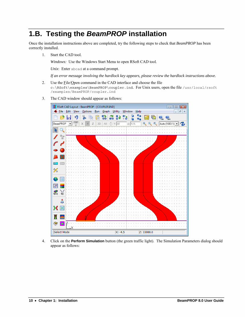
1.B. Testing the BeamPROP installation Once the installation instructions above are completed, try the following steps to check that BeamPROP has been correctly installed.
1. Start the CAD tool.
Windows: Use the Windows Start Menu to open RSoft CAD tool.
Unix: Enter xbcad at a command prompt.
If an error message involving the hardlock key appears, please review the hardlock instructions above.
2. Use the File/Open command in the CAD interface and choose the file c:\RSoft\examples\BeamPROP\coupler.ind. For Unix users, open the file /usr/local/rsoft /examples/BeamPROP/coupler.ind
3. The CAD window should appear as follows:
4. Click on the Perform Simulation button (the green traffic light). The Simulation Parameters dialog should
appear as follows:
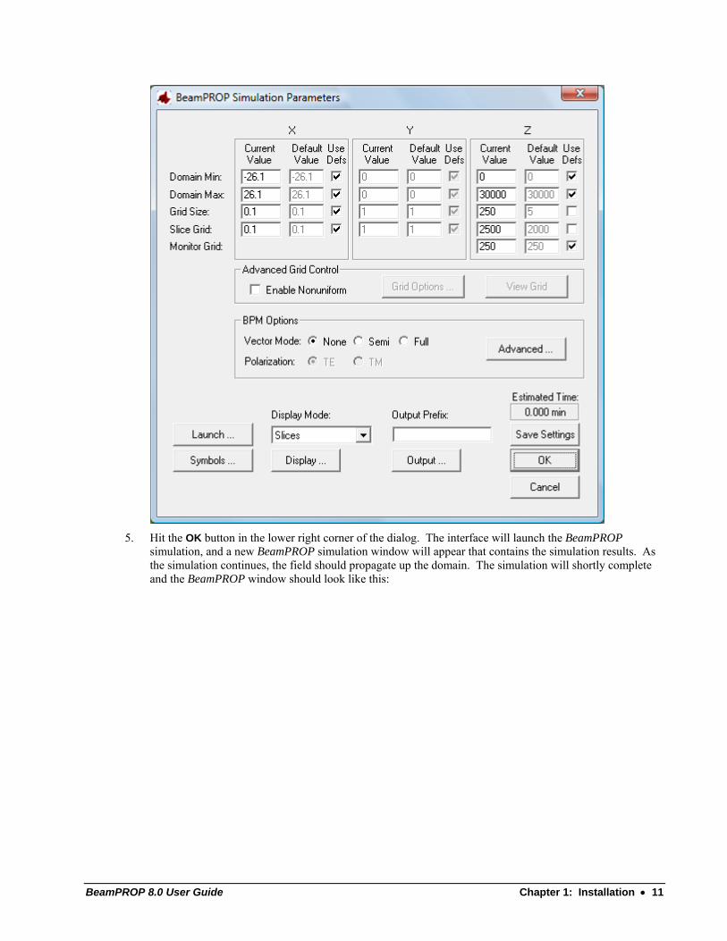
BeamPROP 8.0 User Guide Chapter 1: Installation • 11
5. Hit the OK button in the lower right corner of the dialog. The interface will launch the BeamPROP
simulation, and a new BeamPROP simulation window will appear that contains the simulation results. As the simulation continues, the field should propagate up the domain. The simulation will shortly complete and the BeamPROP window should look like this:
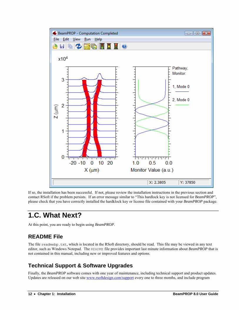
12 • Chapter 1: Installation BeamPROP 8.0 User Guide
If so, the installation has been successful. If not, please review the installation instructions in the previous section and contact RSoft if the problem persists. If an error message similar to “This hardlock key is not licensed for BeamPROP”, please check that you have correctly installed the hardklock key or license file contained with your BeamPROP package.
1.C. What Next? At this point, you are ready to begin using BeamPROP.
README File The file readmebp.txt, which is located in the RSoft directory, should be read. This file may be viewed in any text editor, such as Windows Notepad. The README file provides important last minute information about BeamPROP that is not contained in this manual, including new or improved features and options.
Technical Support & Software Upgrades Finally, the BeamPROP software comes with one year of maintenance, including technical support and product updates. Updates are released on our web site www.rsoftdesign.com/support every one to three months, and include program

BeamPROP 8.0 User Guide Chapter 1: Installation • 13
corrections as well as new features. To access updates, you must contact RSoft after receiving the software to obtain a username and password. Information regarding each update is located in the README file, which can be accessed on the website to determine if you need or want to upgrade, and should be read thoroughly after downloading and installing any update. If you have any questions regarding your maintenance contract, or to renew your maintenance, please contact RSoft Design Group.

BeamPROP 8.0 User Guide Chapter 2: Background • 15
Chapter 2: Background
This chapter provides technical information on the simulation methods used in BeamPROP. This material may be skipped initially, however it introduces terminology and notation which is important for understanding other discussions in the manual.
First, a general background of the BPM algorithm is given. In the following section, the essential numerical methods used in BeamPROP are described in more detail, and further references are given. It should be noted that the actual methods and implementations used in BeamPROP are proprietary adaptations of the following, thus not all details are presented. In the subsequent section, general guidelines for using these numerical methods are given, with particular emphasis on options relevant to BeamPROP. Finally, general guidelines for the selection of numerical parameters are discussed.
2.A. Background The objective of BeamPROP is to provide a general simulation package for computing the propagation of light waves in arbitrary waveguide geometries. This is a complex problem, in general, and several assumptions are made at the outset (many of which are subsequently relaxed). The computational core of the program is based on a finite difference beam propagation method as described in [3,25] and references therein. This technique uses finite difference methods to solve the well-known parabolic or paraxial approximation of the Helmholtz equation. In addition, the program uses "transparent" boundary conditions following [26].
The fundamental physical limitation of the above approach results from the parabolic approximation to the Helmholtz equation, which implies a paraxiality condition on the primary direction of propagation. These limitations can be reduced using more accurate approximations to the Helmholtz equation as outlined in [34]. BeamPROP has the option of implementing this technique, and includes (1,0), (1,1), (2,2), (3,3), and (4,4) Padé approximations.
A second limitation of the above approach results from the assumption of scalar waves, and prevents polarization effects from being considered. BeamPROP Version 2.0, however, introduced several vector beam propagation techniques to overcome this limitation. These methods are based in part on the approach described in [32,41] and related references. Use of this technique is discussed in Section 7.A.
The third key limitation of the BPM approach described above is that it can not account for backward reflections since the one-way wave equation on which it is based does not admit both positive and negative traveling waves. BeamPROP Version 3.0, however, introduced a new bidirectional BPM algorithm as described in [40], which considers coupled forward and backward traveling waves, and can account for reflection phenomenon, including resonant effects as found in grating structures. Use of this technique is discussed in Section 7.B.
The physical propagation problem requires two key pieces of information:
1. The refractive index distribution, n(x,y,z).
2. The input wave field, u(x,y,z=0).
From these, the physics dictates the wave field throughout the rest of the domain, u(x,y,z>0). Naturally, the software provides a way to specify this information; this will be discussed in the following chapters.
16 • Chapter 2: Background BeamPROP 8.0 User Guide
The solution algorithm requires additional input in the form of numerical simulation parameters such as:
• A finite computational domain, {x ∈ (xmin,xmax)}, {y ∈ (ymin,ymax)}, and {z ∈ (zmin,zmax)}.
• The transverse grid sizes, Δx; and Δy.
• The longitudinal step size, Δz.
The software attempts to estimate appropriate values for these parameters, but allows the user to override them. As with any simulation, confidence in the accuracy of the numerical solution requires experimentation to determine the sensitivity to the numerical parameters. For general guidelines on choosing parameters refer to Section 2.C below, as well as the examples in the tutorial chapter and any other notes given throughout the manual.
BeamPROP also has capabilities for computing modes (Chapter 6), handling nonlinear and anisotropic materials (Section 7.E), and incorporating the effects of electrodes and heaters (Section 7.F).
2.B. Review of the Beam Propagation Method (BPM) In this section the concept and capabilities of the beam propagation method, or BPM,[1-3] are reviewed. BPM is the most widely used propagation technique for modeling integrated and fiber optic photonic devices, and most commercial software for such modeling is based on it.
There are several reasons for the popularity of BPM; perhaps the most significant being that it is conceptually straightforward, allowing rapid implementation of the basic technique. This conceptual simplicity also benefits the user of a BPM-based modeling tool as well as the implementer, since an understanding of the results and proper usage of the tool can be readily grasped by a non-expert in numerical methods. In addition to its relative simplicity, BPM is generally a very efficient method, and has the characteristic that its computational complexity can, in most cases, be optimal, that is to say the computational effort is directly proportional to the number of grid points used in the numerical simulation. Another characteristic of BPM is that the approach is readily applied to complex geometries without having to develop specialized versions of the method. Furthermore the approach automatically includes the effects of both guided and radiating fields as well as mode coupling and conversion. Finally, the BPM technique is very flexible and extensible, allowing inclusion of most effects of interest (e.g. polarization, nonlinearities) by extensions of the basic method that fit within the same overall framework.
Numerous applications of BPM to modeling different aspects of photonic devices or circuits have appeared in literature. Examples from the authors’ own experience include various passive waveguiding devices,[4] channel-dropping filters,[5] electro-optic modulators,[6] multimode waveguide devices,[7,8] ring lasers,[9] optical delay line circuits,[10,11] novel y-branches,[12] optical interconnects,[13] polarization splitters,[14] multimode interference devices,[15-19] adiabatic couplers,[20] waveguide polarizers,[21] and polarization rotators.[22] Most of the above references involve experimental demonstrations of novel device concepts designed in whole or in part via BPM.
In the following subsections, the basic ideas involved in the BPM as well as the main extensions to the technique are explained and selected theoretical references are given.
2.B.1. Scalar, Paraxial BPM BPM is essentially a particular approach for approximating the exact wave equation for monochromatic waves, and solving the resulting equations numerically. In this section the basic approach is illustrated by formulating the problem under the restrictions of a scalar field (i.e. neglecting polarization effects) and paraxiality (i.e. propagation restricted to a narrow range of angles). Subsequent sections will describe how these limitations may be removed.
The scalar field assumption allows the wave equation to be written in the form of the well-known Helmholtz equation for monochromatic waves:
( )2, ,2 2 2
22 2+ + k x y z = 0
yx zφ φ φ φ∂ ∂ ∂+
∂ ∂∂
(1)
BeamPROP 8.0 User Guide Chapter 2: Background • 17
Here the scalar electric field has been written as tiezyxtzyxE ωφ −= ),,(),,,( and the notation
( , , ) ( , , )0k x y z = n x y zk has been introduced for the spatially dependent wavenumber, with 20 k π λ= being the wavenumber in free space. The geometry of the problem is defined entirely by the refractive index distribution
),,( zyxn .
Aside from the scalar assumption, the above equation is exact. Considering that in typical guided-wave problems the most rapid variation in the field φ is the phase variation due to propagation along the guiding axis, and assuming that axis is predominantly along the z direction, it is beneficial to factor this rapid variation out of the problem by introducing a so-called slowly varying field u via the ansatz
( ) ( ), , , , i k zx y z u x y z eφ =
(2)
Here k is a constant number to be chosen to represent the average phase variation of the field φ , and is referred to as the reference wavenumber. The reference wavenumber is frequently expressed in terms of a reference refractive index, n , via nkk 0= . Introducing the above expression into the Helmholtz equation yields the following equation for the slowly varying field:
( )2 02 2 2
22222
u u u u ik - uk kz yxz∂∂ ∂ ∂+ + + + =
∂ ∂ ∂ ∂
(3)
At this point the above equation is completely equivalent to the exact Helmholtz equation, except that it is expressed in terms of u. It is now assumed that the variation of u with z is sufficiently slow so that the first term above can be neglected with respect to the second; this is the familiar slowly varying envelope approximation and in this context it is also referred to as the paraxial or parabolic approximation. With this assumption and after slight rearrangement, the above equation reduces to:
( )2 2
2222
u i u u= + + - uk kz 2k yx⎛ ⎞∂ ∂ ∂⎜ ⎟∂ ∂ ∂⎝ ⎠
(4)
This is the basic BPM equation in three dimensions (3D); simplification to two dimensions (2D) is obtained by omitting any dependence on y. Given an input field, u(x,y,z=0), the above equation determines the evolution of the field in the space z>0.
It is important to recognize what has been gained and lost in the above approach. First, the factoring of the rapid phase variation allows the slowly varying field to be represented numerically on a longitudinal grid (i.e. along z) that can be much coarser than the wavelength for many problems, contributing in part to the efficiency of the technique. Second, the elimination of the second derivative term in z reduces the problem from a second order boundary value problem requiring iteration or eigenvalue analysis, to a first order initial value problem that can be solved by simple "integration" of the above equation along the propagation direction z. This latter point is also a major factor in determining the efficiency of BPM, implying a time reduction by a factor of at least of the order of Nz (the number of longitudinal grid points) compared to full numerical solution of the Helmholtz equation.
The above benefits have not come without a price. The slowly varying envelope approximation limits consideration to fields that propagate primarily along the z axis (i.e. paraxiality), and also places restrictions on the index contrast (more precisely, the rate of change of index with z, which is a combination of index contrast and propagation angle). In addition, fields which have a complicated superposition of phase variation, such as exist in multimode devices such as MMI's, may not be accurately modeled if the phase variation is critical to device behavior. A second key issue beyond the above restrictions on the variation of u is that the elimination of the second derivative also eliminates the possibility for backward travelling wave solutions; thus devices for which reflection is significant will not be accurately modeled.
18 • Chapter 2: Background BeamPROP 8.0 User Guide
Fortunately, the above issues, which should be considered inherent in the BPM approach, can be eliminated or significantly relaxed in many problems through the use of so-called wide-angle and bi-directional extensions to BPM discussed below. Other restrictions in the above formulation, such as neglect of polarization and simplification of materials properties (e.g. isotropic, linear), are not specific to the BPM approach. Extension of the formulation to address these situations is also considered in subsequent sections. In the following section the numerical solution of the basic BPM equation derived above is considered.
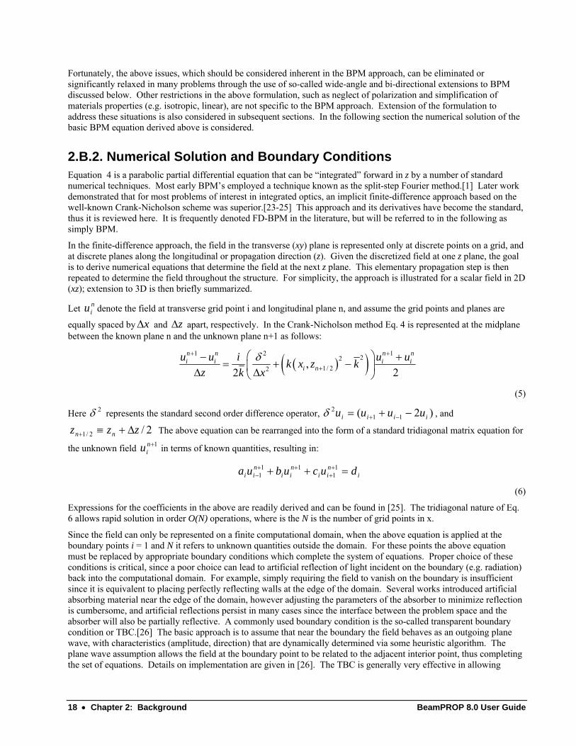
2.B.2. Numerical Solution and Boundary Conditions Equation 4 is a parabolic partial differential equation that can be “integrated” forward in z by a number of standard numerical techniques. Most early BPM’s employed a technique known as the split-step Fourier method.[1] Later work demonstrated that for most problems of interest in integrated optics, an implicit finite-difference approach based on the well-known Crank-Nicholson scheme was superior.[23-25] This approach and its derivatives have become the standard, thus it is reviewed here. It is frequently denoted FD-BPM in the literature, but will be referred to in the following as simply BPM.
In the finite-difference approach, the field in the transverse (xy) plane is represented only at discrete points on a grid, and at discrete planes along the longitudinal or propagation direction (z). Given the discretized field at one z plane, the goal is to derive numerical equations that determine the field at the next z plane. This elementary propagation step is then repeated to determine the field throughout the structure. For simplicity, the approach is illustrated for a scalar field in 2D (xz); extension to 3D is then briefly summarized.
Let niu denote the field at transverse grid point i and longitudinal plane n, and assume the grid points and planes are
equally spaced by xΔ and zΔ apart, respectively. In the Crank-Nicholson method Eq. 4 is represented at the midplane between the known plane n and the unknown plane n+1 as follows:
( )( )1 2 122
1/ 22 ,22
n n n ni i i i
i nu u i u uk x z k
z xkδ+ +
+
⎛ ⎞− += + −⎜ ⎟Δ Δ⎝ ⎠
(5)
Here 2δ represents the standard second order difference operator, )2( 112
iiii uuuu −+= −+δ , and
2/2/1 zzz nn Δ+≡+ The above equation can be rearranged into the form of a standard tridiagonal matrix equation for
the unknown field 1+niu in terms of known quantities, resulting in:
inii
nii
nii ducubua =++ +
+++
−1
111
1
(6)
Expressions for the coefficients in the above are readily derived and can be found in [25]. The tridiagonal nature of Eq. 6 allows rapid solution in order O(N) operations, where is the N is the number of grid points in x.
Since the field can only be represented on a finite computational domain, when the above equation is applied at the boundary points i = 1 and N it refers to unknown quantities outside the domain. For these points the above equation must be replaced by appropriate boundary conditions which complete the system of equations. Proper choice of these conditions is critical, since a poor choice can lead to artificial reflection of light incident on the boundary (e.g. radiation) back into the computational domain. For example, simply requiring the field to vanish on the boundary is insufficient since it is equivalent to placing perfectly reflecting walls at the edge of the domain. Several works introduced artificial absorbing material near the edge of the domain, however adjusting the parameters of the absorber to minimize reflection is cumbersome, and artificial reflections persist in many cases since the interface between the problem space and the absorber will also be partially reflective. A commonly used boundary condition is the so-called transparent boundary condition or TBC.[26] The basic approach is to assume that near the boundary the field behaves as an outgoing plane wave, with characteristics (amplitude, direction) that are dynamically determined via some heuristic algorithm. The plane wave assumption allows the field at the boundary point to be related to the adjacent interior point, thus completing the set of equations. Details on implementation are given in [26]. The TBC is generally very effective in allowing
BeamPROP 8.0 User Guide Chapter 2: Background • 19
radiation to freely escape the computational domain, however there are problems for which it does not perform well. To address this several other boundary conditions have recently been explored.[27-29]
The above numerical solution can be readily extended to 3D, however the direct extension of the Crank-Nicholson approach leads to a system of equations that is not tridiagonal, and requires ( )2 2
x yO N N⋅ operations to solve directly which is non-optimal. Fortunately there is a standard numerical approach referred to as the alternating direction implicit or ADI method,[30] which allows the 3D problem to be solved with optimal ( )x yO N N⋅ efficiency.
In this and the previous section the concept and implementation details of the basic BPM method have been reviewed. In the following sections various methods for extending BPM are summarized, and details of numerical implementation can be found in the corresponding references.
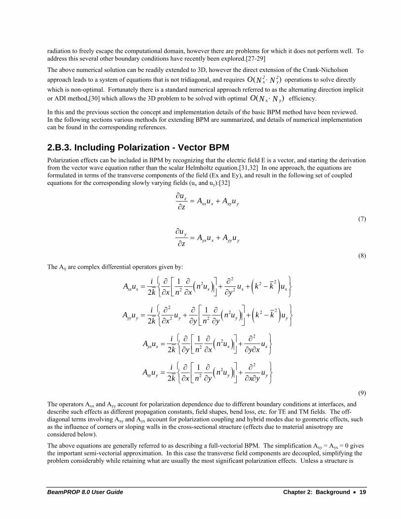
2.B.3. Including Polarization - Vector BPM Polarization effects can be included in BPM by recognizing that the electric field E is a vector, and starting the derivation from the vector wave equation rather than the scalar Helmholtz equation.[31,32] In one approach, the equations are formulated in terms of the transverse components of the field (Ex and Ey), and result in the following set of coupled equations for the corresponding slowly varying fields (ux and uy):[32]
yxyxxxz uAuA
zu
+=∂
∂
(7)
yyyxyxy uAuA
zu
+=∂
∂
(8)
The Aij are complex differential operators given by:
( ) ( )2 22 2
2 21
2xx x x x xiA u n u u k k u
x n x yk⎧ ⎫∂ ∂ ∂⎡ ⎤= + + −⎨ ⎬⎢ ⎥∂ ∂ ∂⎣ ⎦⎩ ⎭
( ) ( )2 22 22 2
12yy y y y yiA u u n u k k u
x y n yk⎧ ⎫⎡ ⎤∂ ∂ ∂
= + + −⎨ ⎬⎢ ⎥∂ ∂ ∂⎣ ⎦⎩ ⎭
( )2
22
12yx x x xiA u n u u
y n x y xk⎧ ⎫∂ ∂ ∂⎡ ⎤= +⎨ ⎬⎢ ⎥∂ ∂ ∂ ∂⎣ ⎦⎩ ⎭
( )2
22
12xy y y yiA u n u u
x n y x yk⎧ ⎫⎡ ⎤∂ ∂ ∂
= +⎨ ⎬⎢ ⎥∂ ∂ ∂ ∂⎣ ⎦⎩ ⎭
(9)
The operators Axx and Ayy account for polarization dependence due to different boundary conditions at interfaces, and describe such effects as different propagation constants, field shapes, bend loss, etc. for TE and TM fields. The off-diagonal terms involving Axy and Ayx account for polarization coupling and hybrid modes due to geometric effects, such as the influence of corners or sloping walls in the cross-sectional structure (effects due to material anisotropy are considered below).
The above equations are generally referred to as describing a full-vectorial BPM. The simplification Axy = Ayx = 0 gives the important semi-vectorial approximation. In this case the transverse field components are decoupled, simplifying the problem considerably while retaining what are usually the most significant polarization effects. Unless a structure is
20 • Chapter 2: Background BeamPROP 8.0 User Guide
specifically designed to induce coupling, the effect of the off-diagonal terms is extremely weak and the semi-vectorial approximation is an excellent one.
2.B.4. Removing Paraxiality – Wide-Angle BPM The paraxiality restriction on the BPM, as well as the related restrictions on index-contrast and multimode propagation noted earlier, can be relaxed through the use of extensions that have been referred to as wide-angle BPM.[33-35] The essential idea behind the various approaches is to reduce the paraxial limitations by incorporating the effect of the
z/u 22 ∂∂ term that was neglected in the derivation of the basic BPM. The different approaches vary in the method and degree of approximation by which they accomplish this. The most popular formulation is referred to as the multistep Padé-based wide-angle technique,[34] and is summarized below.
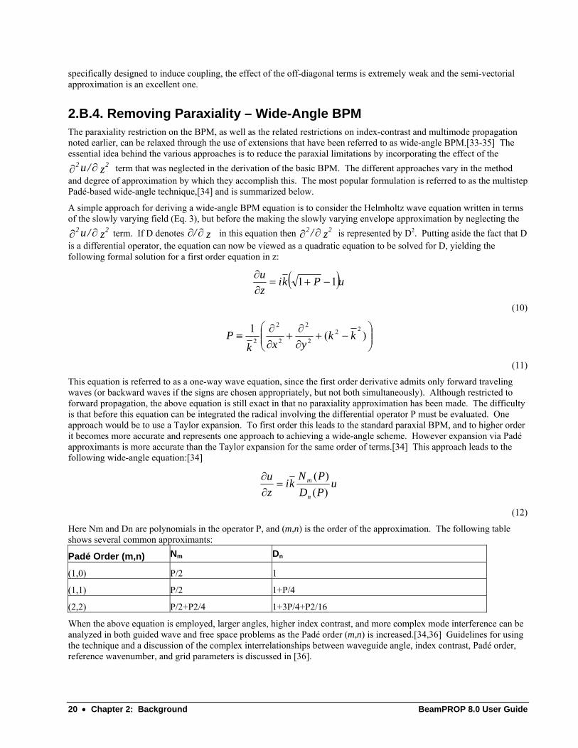
A simple approach for deriving a wide-angle BPM equation is to consider the Helmholtz wave equation written in terms of the slowly varying field (Eq. 3), but before the making the slowly varying envelope approximation by neglecting the
z/u 22 ∂∂ term. If D denotes z/ ∂∂ in this equation then z/ 22 ∂∂ is represented by D2. Putting aside the fact that D is a differential operator, the equation can now be viewed as a quadratic equation to be solved for D, yielding the following formal solution for a first order equation in z:
( )uPkizu 11 −+=
∂∂
(10)
⎟⎟⎠
⎞⎜⎜⎝
⎛−+
∂∂
+∂∂
≡ )(1 222
2
2
2
2 kkyxk
P
(11)
This equation is referred to as a one-way wave equation, since the first order derivative admits only forward traveling waves (or backward waves if the signs are chosen appropriately, but not both simultaneously). Although restricted to forward propagation, the above equation is still exact in that no paraxiality approximation has been made. The difficulty is that before this equation can be integrated the radical involving the differential operator P must be evaluated. One approach would be to use a Taylor expansion. To first order this leads to the standard paraxial BPM, and to higher order it becomes more accurate and represents one approach to achieving a wide-angle scheme. However expansion via Padé approximants is more accurate than the Taylor expansion for the same order of terms.[34] This approach leads to the following wide-angle equation:[34]
uPDPN
kizu
n
m
)()(
=∂∂
(12)
Here Nm and Dn are polynomials in the operator P, and (m,n) is the order of the approximation. The following table shows several common approximants:
Padé Order (m,n) Nm Dn
(1,0) P/2 1
(1,1) P/2 1+P/4
(2,2) P/2+P2/4 1+3P/4+P2/16
When the above equation is employed, larger angles, higher index contrast, and more complex mode interference can be analyzed in both guided wave and free space problems as the Padé order (m,n) is increased.[34,36] Guidelines for using the technique and a discussion of the complex interrelationships between waveguide angle, index contrast, Padé order, reference wavenumber, and grid parameters is discussed in [36].
BeamPROP 8.0 User Guide Chapter 2: Background • 21
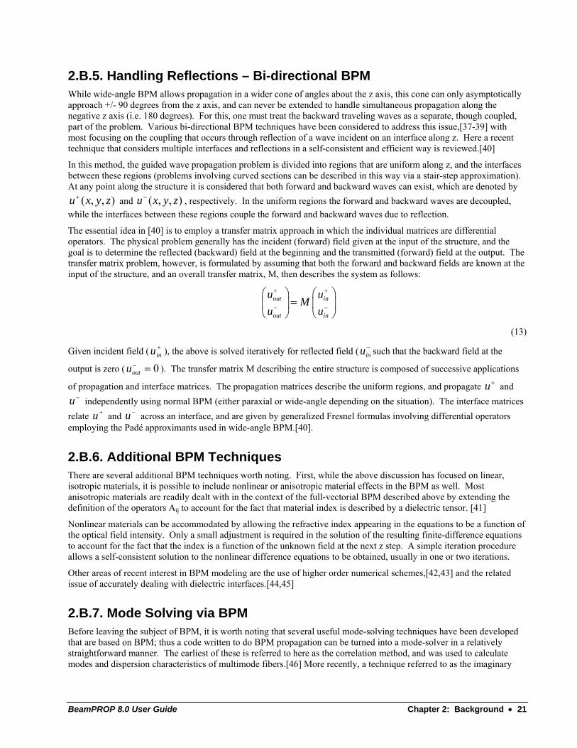
2.B.5. Handling Reflections – Bi-directional BPM While wide-angle BPM allows propagation in a wider cone of angles about the z axis, this cone can only asymptotically approach +/- 90 degrees from the z axis, and can never be extended to handle simultaneous propagation along the negative z axis (i.e. 180 degrees). For this, one must treat the backward traveling waves as a separate, though coupled, part of the problem. Various bi-directional BPM techniques have been considered to address this issue,[37-39] with most focusing on the coupling that occurs through reflection of a wave incident on an interface along z. Here a recent technique that considers multiple interfaces and reflections in a self-consistent and efficient way is reviewed.[40]
In this method, the guided wave propagation problem is divided into regions that are uniform along z, and the interfaces between these regions (problems involving curved sections can be described in this way via a stair-step approximation). At any point along the structure it is considered that both forward and backward waves can exist, which are denoted by
),,( zyxu+ and ),,( zyxu− , respectively. In the uniform regions the forward and backward waves are decoupled, while the interfaces between these regions couple the forward and backward waves due to reflection.
The essential idea in [40] is to employ a transfer matrix approach in which the individual matrices are differential operators. The physical problem generally has the incident (forward) field given at the input of the structure, and the goal is to determine the reflected (backward) field at the beginning and the transmitted (forward) field at the output. The transfer matrix problem, however, is formulated by assuming that both the forward and backward fields are known at the input of the structure, and an overall transfer matrix, M, then describes the system as follows:
out in
out in
u uM
u u
+ +
− −
⎛ ⎞ ⎛ ⎞=⎜ ⎟ ⎜ ⎟
⎝ ⎠ ⎝ ⎠
(13)
Given incident field ( +inu ), the above is solved iteratively for reflected field ( −
inu such that the backward field at the
output is zero ( 0=−outu ). The transfer matrix M describing the entire structure is composed of successive applications
of propagation and interface matrices. The propagation matrices describe the uniform regions, and propagate +u and −u independently using normal BPM (either paraxial or wide-angle depending on the situation). The interface matrices
relate +u and −u across an interface, and are given by generalized Fresnel formulas involving differential operators employing the Padé approximants used in wide-angle BPM.[40].
2.B.6. Additional BPM Techniques There are several additional BPM techniques worth noting. First, while the above discussion has focused on linear, isotropic materials, it is possible to include nonlinear or anisotropic material effects in the BPM as well. Most anisotropic materials are readily dealt with in the context of the full-vectorial BPM described above by extending the definition of the operators Aij to account for the fact that material index is described by a dielectric tensor. [41]
Nonlinear materials can be accommodated by allowing the refractive index appearing in the equations to be a function of the optical field intensity. Only a small adjustment is required in the solution of the resulting finite-difference equations to account for the fact that the index is a function of the unknown field at the next z step. A simple iteration procedure allows a self-consistent solution to the nonlinear difference equations to be obtained, usually in one or two iterations.
Other areas of recent interest in BPM modeling are the use of higher order numerical schemes,[42,43] and the related issue of accurately dealing with dielectric interfaces.[44,45]
2.B.7. Mode Solving via BPM Before leaving the subject of BPM, it is worth noting that several useful mode-solving techniques have been developed that are based on BPM; thus a code written to do BPM propagation can be turned into a mode-solver in a relatively straightforward manner. The earliest of these is referred to here as the correlation method, and was used to calculate modes and dispersion characteristics of multimode fibers.[46] More recently, a technique referred to as the imaginary
22 • Chapter 2: Background BeamPROP 8.0 User Guide
distance BPM has been developed which is generally significantly faster.[47,48] It should be noted that the imaginary distance BPM technique is formally equivalent to many other iterative mode solving techniques;[49,50] the description in terms of BPM is simply a convenience that allows one to leverage existing code and concepts. The results in [50], which can be duplicated via imaginary distance BPM, have shown excellent agreement with other published data.
In both BPM-based mode-solving techniques a given incident field is launched into a geometry that is z-invariant, and some form of BPM propagation is performed. Since the structure is uniform along z, the propagation can be equivalently described in terms of the modes and propagation constants of the structure. Considering 2D propagation of a scalar field for simplicity, the incident field, )(xinφ , can be expanded in the modes of the structure as
( ) ( )in m mm
x c xφ φ= ∑
(14)
The summation should of course consist of a true summation over guided modes and integration over radiation modes, but for brevity the latter is not explicitly shown. Propagation through the structure can then be expressed as
( ) ( ), mi zm m
mx z c x e βφ φ= ∑
(15)
In each BPM-based mode-solving technique, the propagating field obtained via BPM is conceptually equated with the above expression to determine how to extract mode information from the BPM results.
As the name implies, in the imaginary distance BPM the longitudinal coordinate z is replaced by z'=iz, so that propagation along this imaginary axis should follow
( ) ( ) ', ' m zm m
mx z c x eβφ φ= ∑
(16)
The propagation implied by the exponential term in Eq. 15 has become exponential growth in Eq. 16, with the growth rate of each mode being equal to its real propagation constant. The essential idea of the method is to launch an arbitrary field, say a Gaussian, and propagate the field through the structure along the imaginary axis. Since the fundamental mode (m=0) has by definition the highest propagation constant, its contribution to the field will have the highest growth rate and will dominate all other modes after a certain distance, leaving only the field pattern )(0 xφ , The propagation constant can then be obtained by the following variational-type expression:
*
2*
22
2 + dxkx
dx
φφ φβ
φ φ
⎛ ⎞∂⎜ ⎟∂⎝ ⎠=
∫∫
(17)
Higher order modes can be obtained by using an orthogonalization procedure to subtract contributions from lower order modes while performing the propagation.[51] Issues such as optimal choice of launch field, reference wavenumber, and step size are discussed in [48,50]. Also, an additional correction is added which removes the error due to the fact that we have solved for the eigenvalues of the paraxial
It is important to note that the imaginary distance BPM is not the same as the common technique of performing a standard propagation and waiting for the solution to reach steady state. The latter will only obtain the fundamental mode if the structure is single mode, and generally takes longer to converge. The imaginary distance BPM is closely related to the shifted inverse power method for finding eigenvalues and eigenvectors of a matrix.
In the correlation method, an arbitrary field is launched into the structure and propagated via normal BPM. During the propagation the following correlation function between the input field and the propagating field is computed:
BeamPROP 8.0 User Guide Chapter 2: Background • 23
( ) ( ) ( )* ,inP z x x z dxφ φ= ∫
(18)
Using Eq. 14 and Eq. 15, the correlation function can also be expressed as:
( ) 2mi z
mm
P z c e β= ∑
(19)
From this expression one can see that a Fourier transform of the computed correlation function should have a spectrum with peaks at the modal propagation constants. The corresponding modal fields can be obtained with a second propagation by beating the propagating field against the known propagation constants via:
( ) ( )0
1 , m
Li z
m x x z eL
βφ φ −= ∫
(20)
Several corrections to the propagation constants can be made:
• A correction is made which accounts for the error introduced by solving the paraxial equation, and not the exact Helmholtz equation. Further details on the technique are found in [46].
• Second, the imaginary part of the propagation constant can be found by substituting the mode profile in the wave equation and solving for the propagation constant. This not only results in an imaginary value, but a corrected real value as well.
While the correlation method is generally slower than the imaginary distance BPM, it has the advantage that it is sometimes applicable to problems that are difficult or impossible for imaginary distance BPM, such as leaky or radiating modes.
2.B.8. References [1] M.D. Feit and J.A. Fleck, “Light propagation in graded-index optical fibers”, Appl. Opt. 17, 3990 (1978).
[2] See references in D. Yevick, “A guide to electric field propagation techniques for guided-wave optics”, Opt. and Quant. Elec. 26, S185 (1994).
[3] R. Scarmozzino, A. Gopinath, R. Pregla, and S. Helfert, “Numerical Techniques for Modeling Guided-Wave Photonic Devices,” J. Selected Topics in Quantum Electronics 6, 150 (2000).
[4] L. Eldada, M.N. Ruberto, R. Scarmozzino, M. Levy, and R.M. Osgood, Jr., “Laser-Fabricated Low-Loss Single-Mode Waveguiding Devices in GaAs”, J. Lightwave Tech. 10, 1610 (1992).
[5] M. Levy, L. Eldada, R. Scarmozzino, R.M. Osgood, Jr., P.S.D. Lin, and F. Tong, “Fabrication of Narrow-Band Channel-Dropping Filters”, Photon. Tech. Lett. 4, 1378 (1992).
[6] L. Eldada, M.N. Ruberto, M. Levy, R. Scarmozzino, and R.M. Osgood, Jr., “Rapid Direct Fabrication of Active Electro-Optic Modulators in GaAs”, J. Lightwave Tech. 12, 1588 (1994).
[7] I. Ilic, R. Scarmozzino, R.M. Osgood, Jr., J.T. Yardley, K.W. Beeson, and M.J. McFarland, “Modeling Multimode-Input Star Couplers in Polymers”, J. Lightwave Tech. 12, 996 (1994).
[8] I. Ilic, R. Scarmozzino, R.M. Osgood, Jr., J.T. Yardley, K.W. Beeson, and M.J. McFarland, and J. Schweyen, “Photopattermed Polymer Multimode 8x8 Star Couplers: Comparative Design Methodologies and Device Measurements”, IEICE Trans. Commun. E80-B (1997).
[9] M.C. Shih, M. Hu, M.B. Freiler, M. Levy, R. Scarmozzino, R.M. Osgood, Jr., I.W. Tao, and W.I. Wang, “Fabrication of an InGaAs SQW Circular Ring Laser By Direct Laser Patterning”, Appl. Phys. Lett. 66, 2608 (1995).

24 • Chapter 2: Background BeamPROP 8.0 User Guide
[10] L. Eldada, R. Scarmozzino, R.M. Osgood, Jr., D.C. Scott, Y. Chang, and H.R. Fetterman, “Laser-Fabricated Delay Lines in GaAs for Optically-Steered Phased-Array Radar”, J. Lightwave Tech. 13, 2034 (1995).
[11] M.H. Hu, Z. Huang, K.L. Hall, R. Scarmozzino, and R.M. Osgood, Jr., “An Integrated Two-Stage Cascaded Mach–Zehnder Device in GaAs”, J. Lightwave Tech. 16, 1447 (1998).
[12] M. Hu, R. Scarmozzino, M. Levy, and R.M. Osgood, Jr., “A low-loss and compact waveguide y-branch using refractive index tapering”, Photon. Tech. Lett., 9, 203 (1997).
[13] R. Scarmozzino, R.M. Osgood, Jr., L. Eldada, J.T. Yardley, Y. Liu, J. Bristow, J. Stack, J. Rowlette, and Y.S. Liu, “Design and Fabrication of Passive Optical Components for Multimode Parallel Optical Links”, SPIE Photonic West Meeting, San Jose, CA, 3005, 257 (1997).
[14] M. Hu, J.Z. Huang, R. Scarmozzino, M. Levy, and R.M. Osgood, Jr., “Tunable Mach-Zehnder polarization splitter using height-tapered y-branches”, Photon. Tech. Lett. 9, 773 (1997).
[15] D.S. Levy, Y.M. Li, R. Scarmozzino, and R.M. Osgood, Jr., “A Multimode Interference-Based Variable Power Splitter in GaAs–AlGaAs”, Photon. Tech. Lett. 9, 1373 (1997).
[16] D.S. Levy, R. Scarmozzino, Y.M. Li, and R.M. Osgood, Jr., “A New Design for Ultracompact Multimode Interference-Based 2x2 Couplers”, Photon. Tech. Lett. 10, 96 (1998).
[17] J. Z. Huang, M. H. Hu, J. Fujita, R. Scarmozzino, and R. M. Osgood, Jr., “High-Performance Metal-Clad Multimode Interference Devices for Low-Index-Contrast Material Systems”, Photon. Tech. Lett. 10, 561 (1998).
[18] J. Z. Huang, R. Scarmozzino, and R. M. Osgood, Jr., “A New Design Approach to Large Input/Output-Number Multimode Interference Couplers and Its Application to Low-Crosstalk WDM Routers”, Photon. Tech. Lett. 10, 1292 (1998).
[19] D.S. Levy, K.H. Park, R. Scarmozzino, R.M. Osgood, Jr., C. Dries, P. Studenkov, and S. Forrest, “Fabrication of ultracompact 3-dB 2x2 MMI power splitters”, Photon. Tech. Lett. 11, 1009 (1999).
[20] T.A. Ramadan, R. Scarmozzino, and R.M. Osgood, Jr., “Adiabatic Couplers: Design Rules and Optimization”, J. Lightwave Tech. 16, 277 (1998).
[21] J. Fujita, M. Levy, R. Scarmozzino, R.M. Osgood, Jr., L. Eldada, and J.T. Yardley, “Integrated Multistack Waveguide Polarizer”, Photon. Tech. Lett. 10, 93 (1998).
[22] J. Z. Huang, R. Scarmozzino, G. Nagy, M. J. Steel and R. M. Osgood, Jr., “Realization of a compact and single-mode optical passive polarization converter”, Photon. Tech. Lett. 12, 317 (2000).
[23] D. Yevick and B. Hermansson, “Efficient beam propagation techniques”, J. Quantum Electron. 26, 109 (1990).
[24] Y. Chung and N. Dagli, “An assessment of finite difference beam propagation method”, J. Quantum Electron 26, 1335 (1990).
[25] R. Scarmozzino and R.M. Osgood, Jr., “Comparison of finite-difference and Fourier-transform solutions of the parabolic wave equation with emphasis on integrated-optics applications”, J. Opt. Soc. Amer. A 8, 724 (1991).
[26] G.R. Hadley, “Transparent boundary condition for the beam propagation method”, Opt. Lett. 16, 624, (1991); G.R. Hadley, “Transparent boundary condition for the beam propagation method”, J. Quantum Electron 28, 363 (1992).
[27] C. Vassalo and F. Collino, “Highly efficient absorbing boundary condition for the beam propagation method”, J. Lightwave Technol.14, 1570 (1996).
[28] W.P. Huang, C.L. Xu, W. Lui, and K. Yokoyama, “The perfectly matched layer (PML) boundary condition for the beam propagation method”, Photon. Technol. Lett. 8, 649 (1996).
[29] Y.P. Chiou and H.C. Chang, “Complementary operators method as the absorbing boundary condition for the beam propagation method”, Photon. Technol. Lett. 8, 976 (1998).
[30] W.H. Press, B.P. Flannery, S.A. Teuklsky, and W.T. Vetterling, Numerical Recipes: The Art of Scientific Computing, (Cambridge Univ., New York, 1986).
[31] R. Clauberg and P. Von Allmen, “Vectorial beam propagation method for integrated optics”, Electron. Lett. 27, 654 (1991).
BeamPROP 8.0 User Guide Chapter 2: Background • 25
[32] W.P. Huang and C.L. Xu, “Simulation of three-dimensional optical waveguides by a full-vector beam propagation method”, J. Quantum Electron. 29, 2639 (1993).
[33] D. Yevick and M. Glasner, “Analysis of forward wide-angle light propagation in semiconductor rib waveguides and integrated-optic structures”, Electron. Lett. 25, 1611 (1989).
[34] G.R. Hadley, “Wide-angle beam propagation using Pade approximant operators”, Optics Letters 17, 1426, (1992); G.R. Hadley, “Multistep method for wide-angle beam propagation”, Optics Letters 17, 1743 (1992).
[35] H.J.W.M. Hoekstra, G.J.M. Krijnen, and P.V. Lambeck, “New formulations of the beam propagation method based on the slowly varying envelope approximation”, Optics Communications, 97, 301 (1993).
[36] I. Ilic, R. Scarmozzino, and R.M. Osgood, Jr., “Investigation of the Pade approximant-based wide-angle beam propagation method for accurate modeling of waveguiding circuits”, J. Lightwave Technol. 14, 2813 (1996).
[37] P. Kaczmarski and P.E. Lagasse, “Bidirectional beam propagation method”, Electron. Lett. 24, 675 (1988).
[38] Y. Chung and N. Dagli, “Modeling of guided-wave optical components with efficient finite-difference beam propagation methods”, Tech. Dig. IEEE AP-S Int. Symp., 1992 1, 248 (1992).
[39] Y. Chiou and H. Chang, “Analysis of optical waveguide discontinuities using the Pade approximants”, Photon. Technol. Lett. 9, 964 (1997).
[40] H. Rao, R. Scarmozzino, and R.M. Osgood, Jr., “A bidirectional beam propagation method for multiple dielectric interfaces”, Photon. Technol. Lett. 11,830 (1999).
[41] C.L. Xu, W.P. Huang, J. Chrostowski, and S.K. Chaudhuri, “A full-vectorial beam propagation method for anisotropic waveguides”, J. Lightwave Tech. 12, 1926 (1994).
[42] J. Yamauchi, J. Shibayama, and H. Nakano, “Modified finite-difference beam propagation method based on the generalized Douglas scheme for variable coefficients”, Photon. Technol. Lett. 7, 661 (1995).
[43] G.R. Hadley, “Low-truncation-error finite difference equations for photonics simulation I: beam propagation”, J. Lightwave Technol. 16, 134 (1998).
[44] H.J.W.M. Hoekstra, G.J.M. Krijnen, and P.V. Lambeck, “Efficient interface conditions for the finite difference beam propagation method”, J. Lightwave Technol. 10, 1352 (1992).
[45] J. Yamauchi, M. Sekiguchi, O. Uchiyama, J. Shibayama, and H. Nakano, “Modified finite-difference formula for the analysis of semivectorial modes in step-index optical waveguides”, Photon. Technol. Lett. 9, 961 (1997).
[46] M.D. Feit and J.A. Fleck, “Computation of mode properties in optical fiber waveguides by a propagating beam method”, Applied Optics, 19, 1154 (1980).
[47] D. Yevick and B. Hermansson, “New formulations of the matrix beam propagation method: Application to rib waveguides”, J. Quantum Electron., 25, 221 (1989).
[48] S. Jungling and J.C. Chen, “A study and optimization of eigenmode calculations using the imaginary-distance beam-propagation method”, J. Quantum Electron. 30, 2098 (1994).
[49] D. Yevick and Witold Bardyszewski, “Correspondence of variational finite-difference (relaxation) and imaginary-distance propagation methods for modal analysis”, Opt. Lett. 17, 329 (1992).
[50] G.R. Hadley and R.E. Smith, “Full-vector waveguide modeling using an iterative finite-difference method with transparent boundary conditions”, J. Quantum Electron. (1995).
[51] J.C. Chen and S. Jungling, “Computation of higher-order waveguide modes by the imaginary-distance beam propagation method”, Optical and Quantum Electron. 26, S199 (1994).
2.C. General guidelines for Using BPM In this section several general guidelines for using BPM, including choosing relevant numerical simulation parameters, are given. While the discussion for the most part applies to BPM in general, some of the comments and terminology are specific to BeamPROP.

26 • Chapter 2: Background BeamPROP 8.0 User Guide
2.C.1. Overview The guidelines for using BPM presented in this section consider several parameters or options that can be chosen when performing the simulation, and the influences that these parameters have on the results of the calculation. The parameters and influences considered in each section are as noted below. Also noted is an expression for the scaling of the simulation time, since choosing numerical parameters is always in some sense a tradeoff between accuracy/stability and computational resources.
Parameters: Grid Sizes, Δx and Δy
Step Size, Δz
Reference Wavenumber, k
Pade Order
Computational Domain / Boundary Conditions
Polarization Options
Scheme Parameter (Full-Vector BPM only)
Influences: Accuracy/Stability of BPM
Accuracy/Stability of Mode Solving
Accuracy/Stability of Boundary Conditions
Computation Time: Approximately proportional to Nx*Ny*Nz*m,
where Nx = (domain in x)/Δ x, etc. and m is the first number in the Pade Order
Full-vector BPM is approximately 4 times scalar or semi-vector normal BPM
Bi-directional BPM is N times normal BPM, where N is the number of iterations (2-100)
2.C.2. General Philosophy for Choosing Parameters If estimated time with BeamPROP defaults is “reasonable”, start with the defaults and then “refine” as needed to obtain accuracy, or “coarsen” to optimize performance if many runs are to be done.
If not, coarsen the defaults until the time is reasonable, and run the problem to see if it makes physical sense. Then refine as needed to obtain accuracy.
Effect of Grid Sizes (Δx and Δy) Smaller grid sizes improve the accuracy of both BPM and mode solving. Stability is not affected except in the case of full-vector BPM.
Smaller grid sizes produce difficulty with transparent boundary conditions (unwanted reflections) or with fields at interfaces (artifacts such as energy “stuck” near an interface). These problems are alleviated with the use of smaller step size.
Effect of Step Size (Δz) BPM and mode solving based on normal BPM (i.e. correlation method)
BeamPROP 8.0 User Guide Chapter 2: Background • 27
• Smaller step size improves accuracy; stability is unaffected.
• Smaller step size also alleviates performance problems of transparent boundary conditions and propagation near interfaces at small grid sizes.
• To some extent, the step size can be traded against the reference wavenumber, since accuracy is in part related to:
( )k k zz− ⋅ Δ
Mode solving based on imaginary distance BPM. (i.e. iterative method)
• Smaller step size has no significant effect on accuracy/stability.
• Larger step size improves rate of convergence, but too large a step size causes convergence to unwanted modes. BeamPROP chooses a default near this limit; if problems occur, reduce the step size by factors of 2 until the problems resolves.
Effect of Reference Wavenumber BPM and mode solving based on normal BPM (i.e. correlation method)
• More accurate reference wavenumber (i.e. k close to kZ, where kZ represents actual behavior of field) leads to more accurate results. Best choice is usually θβ cos , where β is the propagation constant of the main mode involved in the propagation, and θ is the angle of propagation relative to the z axis.
• To some extent, the reference wavenumber can be traded against the step size, since accuracy is in part related to
( )k k zz− ⋅ Δ
• Similarly (for BPM only), to some extent the reference wavenumber can be traded against the Pade Order, since higher Pade Order reduces the effect of the above error term.
Mode solving based on imaginary distance BPM (i.e. iterative method)
Reference wavenumber choice has no significant effect, since internally it is updated dynamically to match mode. Best initial choice is the default, kext.
Effect of Pade Order Normal BPM
• Higher Pade Order improves accuracy at “large” angles, “large” index contrast, and when a “large” range of propagation constants is involved (e.g. multimode devices). The three parameters are intermixed, making it impossible to say what is “large” in general.
• The effect of Pade Order is also intermixed with the effect of the grid and step sizes, as well as the reference wavenumber. A careful convergence study must be undertaken to optimize all the parameters.
Mode Solving (either method)
• Higher Pade Order has no effect on accuracy and should not be used.
Effect of Computational Domain / Boundary Conditions The effect of these options is generally less critical, since the transparent boundary condition (TBC), when it is working properly, should make the effect of the boundary position immaterial. However there are several caveats for each.
Computational Domain
• When the TBC has difficulty, it can sometimes help to choose a larger computational domain.

28 • Chapter 2: Background BeamPROP 8.0 User Guide
• Even if the TBC is working properly, and the field is accurately being calculated in the domain, if you are computing overlap integrals (e.g. via monitors) with fields that significantly extend beyond the domain, the results may not be accurate. In this case, extend the domain to encompass the important fields.
Boundary Conditions
• There are two forms of the TBC, Full and Simple. The default Full TBC attempts to be more intelligent, and is sometimes more accurate, but is sometimes fooled and performs worse than the Simple TBC. When having difficulties, particularly with multimode problems or problems with large amounts of radiation, the Simple TBC should be tried, followed by choosing a smaller step size. If these fail, BeamPROP has several undocumented options which control finer aspects of the transparent boundary conditions; contact RSoft for additional information.
Effect of Polarization Options The primary polarization options are None (i.e. scalar), Semi-Vector, and Full-Vector, and affect the accuracy with which BPM can treat certain effects as noted below. Section 7.A should be read for additional detail on these and other options which control simulation of polarization before doing any simulation involving polarization.
A general guideline is to start with scalar simulations, even if your problem requires more sophistication, and only after your problem starts making sense, work your way up to semi- or full-vector as needed.
• None (Scalar): Polarization effects are ignored. This is appropriate for “small” index contrast such that polarization effects are “weak”, or as a starting point to determine whether a device concept (not based on polarization) will work in principle.
• Semi-Vector: Polarization dependent effects are included, but polarization coupling and hybrid polarization effects are ignored. This is appropriate and sufficient for almost all “large” index contrast problems for which polarization effects are of interest. Simulations are only slightly more complicated and time-consuming than the scalar case.
• Full-Vector: All polarization effects are included, but simulations are significantly more complicated and time consuming than the scalar or semi-vector case. Generally not much more information is obtained, except for devices designed to couple polarizations. Stability is an issue and is controlled by the scheme parameter (see next section).
Effect of Scheme Parameter The scheme parameter should only be used for full-vector simulations to control stability, which becomes an issue for “large” index contrast and/or “small” grid sizes.
To overcome the above instability, the scheme parameter must be set to a value greater than its default of 0.5, and less than 1.0.
A side effect of using a scheme parameter is artificial numerical dissipation; an eigenmode launched into the structure will attenuate instead of propagating without loss. To minimize this dissipation, choose a scheme parameter as close to 0.5 as possible while maintaining stability. To reduce the dissipation at a given scheme parameter, reduce the step size Δz.

BeamPROP 8.0 User Guide Chapter 3: A First Tour of BeamPROP • 29
Chapter 3: A First Tour of BeamPROP
This chapter provides a general overview of the BeamPROP software and its use. We will describe the various programs that make up the package, including their functions and how to run them through both the Graphical User Interface (GUI) and Command Line Interface (CLI)
As noted earlier, BeamPROP uses the RSoft CAD Environment for performing device layout and controlling the simulation. For information about the creation of design files in the CAD, please consult the CAD manual.
3.A. Component Programs and Files After completing the installation procedures described in Chapter 1, the CAD package, the BeamPROP simulation module and examples, and the accompanying WinPLOT technical graphing package will have been placed on your hard disk.
The installation directory (referred to as <rsoft_dir>) of the RSoft Photonics Suite contains several subdirectories. The most important subdirectories will be described in this section; the other sub directions are described in the RSoft Installation Guide.
3.A.1. Component Executables The subdirectory <rsoft_dir>\bin contains the following executable files, among others. Linux users can find the corresponding executable names in the Preface. Executable Description
bcadw32.exe This file is the Windows version of the RSoft CAD. This is the main control program for BeamPROP, and is usually started from the Start menu on the taskbar. Please refer to your operating system manual for information on general procedures for starting programs.
bsimw32.exe This file is the Windows version of the BeamPROP Simulation Program, and is launched automatically by the main program whenever you initiate a simulation.
winplot.exe This file is the Windows version of the WinPLOT technical graphing package. Please consult the WinPLOT manual for more information on its proper usage.
These programs can be run from the command line and used in batch or zcript files in order to initiate a series of simulations automatically. See the next section for details.
30 • Chapter 3: A First Tour of BeamPROP BeamPROP 8.0 User Guide
3.A.2. Example Files The subdirectory <rsoft_dir>\examples\BeamPROP contains example files for BeamPROP. These files have an extension *.ind (named for the refractive index distribution which describes the circuit). A partial listing of these files is as follows:
Example File Description
autoscan.ind A y-branch setup for automatic parameter scanning branch.ind A simple y-branch structure coupler.ind A directional coupler fullvect.ind A full vector waveguide mode calculation (3D) electrod.ind A Mach-Zehnder modulator using electrodes grating.ind A grating structure demonstrating bidirectional BPM guass.ind A Gaussian beam diffracting in free space lens.ind A diffracting Gaussian beam focused by a lens machzndr.ind A Mach-Zehnder modulator in the off state modes2d.ind A slab waveguide setup for mode calculations (2D) modes3d.ind An optical fiber setup for mode calculations (3D) qcoupl3d.ind A pair of coupled waveguides in 3D Fiber or Rib geometry switches.ind An array of directional coupler switches userprof.ind A single waveguide with a user-defined index profile xcoupl3d.ind A crossed pair of waveguides using 3D Multilayer geometry
In addition to these examples, there is a Tutorials subdirectory which contains the index files described in the Tutorial chapters of this manual.
Running an Example The structures described by these files can be viewed by selecting File/Open from within the main program, and choosing the desired index file from the dialog that appears. A simulation can be initiated by clicking on the Perform Simulation (green light) icon, and pressing OK in the simulation parameters dialog.
Alternatively, a simulation can be started from command line by going into the examples directory, and typing bsimw32 followed by the name of the desired index file (the *.ind extension is optional).
If you would like an example for a specific problem, contact RSoft by faxing or e-mailing a complete description of the problem and we will create an appropriate example file to assist you if possible.
3.B. Program Operation A BeamPROP simulation can be started via either the Graphical User Interface (GUI) or a command line interface. Both of these methods are equally powerful, and are useful in different circumstances. Beginning users are encouraged to use BeamPROP via the GUI interface in order to understand the usage of the program. Advanced users who with to incorporate BeamPROP into scripts/batch operations are encouraged to use the scripting capabilities of BeamPROP.

BeamPROP 8.0 User Guide Chapter 3: A First Tour of BeamPROP • 31
3.B.1. GUI Program Operation The GUI operation of BeamPROP is a very straightforward process, and can be broken down into 5 basic steps:
Step 1: Laying out the structure We begin by assuming that a CAD window has been started, and that a layout window has been opened which contains the circuit to be simulated; this could be a newly created circuit, or a previously saved circuit that was loaded via the File/Open menu item. The general operation of the CAD program is described in the RSoft CAD manual.
Step 2: Choosing the BeamPROP simulation engine The first step in initiating a BeamPROP simulation is to ensure that the Simulation Tool has been set to BeamPROP/BPM in the Global Settings dialog box. This indicates to the CAD program that a BeamPROP BPM simulation engine is to be used, rather than another of RSoft’s simulation engines.
Figure 3-1: The Simulation Tool option as shown in the Global Settings dialog box.
Step 3: Setting up the Simulation Parameters The next step in initiating a simulation is to click on Perform Simulation, or green light icon, in the left toolbar. This brings up the simulation parameters dialog as shown in Fig. 3- 2. This dialog allows the basic parameters required for a numerical simulation to be entered, and controls other important aspects of the simulation as well. For clarity in understanding the basic procedures, the detailed description of the input fields for this complex dialog is relegated to the next sections.
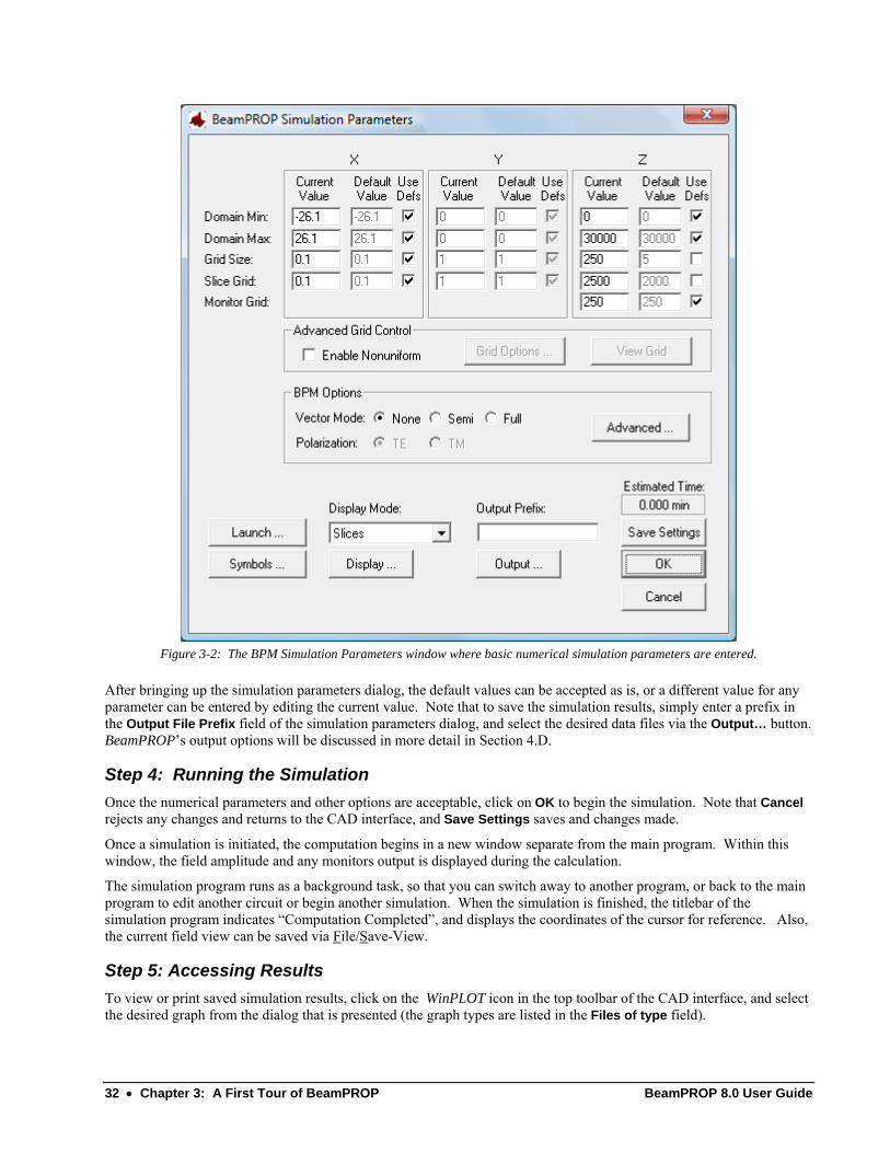
32 • Chapter 3: A First Tour of BeamPROP BeamPROP 8.0 User Guide
Figure 3-2: The BPM Simulation Parameters window where basic numerical simulation parameters are entered.
After bringing up the simulation parameters dialog, the default values can be accepted as is, or a different value for any parameter can be entered by editing the current value. Note that to save the simulation results, simply enter a prefix in the Output File Prefix field of the simulation parameters dialog, and select the desired data files via the Output… button. BeamPROP’s output options will be discussed in more detail in Section 4.D.
Step 4: Running the Simulation Once the numerical parameters and other options are acceptable, click on OK to begin the simulation. Note that Cancel rejects any changes and returns to the CAD interface, and Save Settings saves and changes made.
Once a simulation is initiated, the computation begins in a new window separate from the main program. Within this window, the field amplitude and any monitors output is displayed during the calculation.
The simulation program runs as a background task, so that you can switch away to another program, or back to the main program to edit another circuit or begin another simulation. When the simulation is finished, the titlebar of the simulation program indicates “Computation Completed”, and displays the coordinates of the cursor for reference. Also, the current field view can be saved via File/Save-View.
Step 5: Accessing Results To view or print saved simulation results, click on the WinPLOT icon in the top toolbar of the CAD interface, and select the desired graph from the dialog that is presented (the graph types are listed in the Files of type field).
BeamPROP 8.0 User Guide Chapter 3: A First Tour of BeamPROP • 33
Each output is contained in two ASCII files: one file contains the raw data, and the other contains WinPLOT plotting commands. The file chosen via the above method is the WinPLOT command file so as to correctly display the raw data. To access the raw data, the data file can be opened in any text editor.
3.B.2. CLI Operation As an alternative to using the main BeamPROP program to initiate a simulation, it can sometimes be useful to run the simulation program from the command line. This is particularly true when a series of simulations needs to be run in which some parameter is to be varied, or when incorporating BeamPROP into a larger scripting environment. In this case a batch file can be used to automatically initiate each simulation in turn, without user intervention, freeing the user to perform other tasks.
When operating BeamPROP from the command line, it is important to note that the user can access the exact same feature set as if they were running BeamPROP through the GUI. All simulation options within the GUI are controlled by variables. A list of variables can be found in Appendix C.
Program Syntax The simulation program can be started from the command line with the same functionality as the GUI version.
The standard syntax is the program name, bsimw32, followed by the index file name, and optionally by a series of variable assignments of the form name=value. The syntax is thus:
bsimw32 index-file-name [name=value name=value ...]
A simulation of the circuit is immediately initiated using any parameters stored in the index file, along with any additional parameters specified on the command line (which override those in the index file). The parameters are the same as those used in the main program, and correspond to the input fields documented in the next section. The pre-defined variable names are documented in Appendix C. In addition, any user-defined variable names can also be used in a parameter specification.
Batch File Operation As noted above, a benefit of command line usage is the ability to use batch files to automate a series of simulations. For example, assume that a circuit has been stored in the file wg.ind, and that it is desired to initiate a series of simulations with step sizes of 1, 2, and 5 μ, storing the results in files beginning with the names myruna, myrunb, and myrunc respectively. This might be done under Windows by creating a batch file called runall.bat containing the lines:
start /w bsimw32 wg prefix=myruna step_size=1 slice_display_mode=0 wait=0
start /w bsimw32 wg prefix=myrunb step_size=2 slice_display_mode=0 wait=0
start /w bsimw32 wg prefix=myrunc step_size=5 slice_display_mode=0 wait=0
In the above, the start /w command is used to start the program bsimw32.exe and wait for it to complete before proceeding to the next line in the batch file. The word delay is the name of the index file (without the .ind extension which is optional). The prefix parameter specifies the name to be used for any output files that may be generated, which will be differentiated by their extension, and is equivalent to entering an Output File Prefix in the GUI. Note the prefix must not include an extension. The step_size parameter sets the Z step size for the simulation to the indicated value. Finally, the slice_display_mode=0 specification disables graphing for quiet operation, and wait=0 causes the program to exit immediately after completing the simulation instead of waiting for the user to close the program. To execute the batch file, simply type runall at a DOS prompt.
The above example is intended to illustrate how to use the operating systems native batch capability for performing a series of simulations. Alternatively, BeamPROP provides its own built-in scripting capability to achieve this task which

34 • Chapter 3: A First Tour of BeamPROP BeamPROP 8.0 User Guide
has several advantages, including platform-independence and the fact that the program does not have to be constantly reloaded into memory for each simulation. Furthermore, BeamPROP provides an automated approach generating and running scripts. These capabilities are described in the RSoft CAD manual.
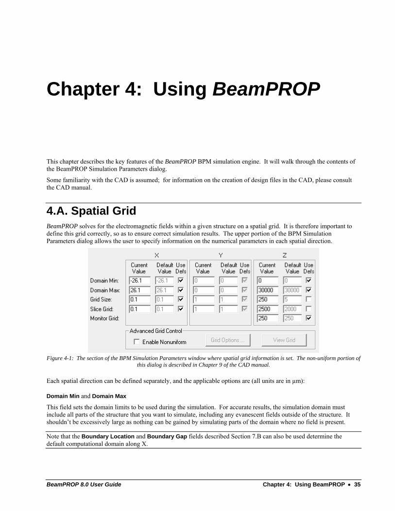
BeamPROP 8.0 User Guide Chapter 4: Using BeamPROP • 35
Chapter 4: Using BeamPROP
This chapter describes the key features of the BeamPROP BPM simulation engine. It will walk through the contents of the BeamPROP Simulation Parameters dialog.
Some familiarity with the CAD is assumed; for information on the creation of design files in the CAD, please consult the CAD manual.
4.A. Spatial Grid BeamPROP solves for the electromagnetic fields within a given structure on a spatial grid. It is therefore important to define this grid correctly, so as to ensure correct simulation results. The upper portion of the BPM Simulation Parameters dialog allows the user to specify information on the numerical parameters in each spatial direction.
Figure 4-1: The section of the BPM Simulation Parameters window where spatial grid information is set. The non-uniform portion of
this dialog is described in Chapter 9 of the CAD manual.
Each spatial direction can be defined separately, and the applicable options are (all units are in µm):
Domain Min and Domain Max
This field sets the domain limits to be used during the simulation. For accurate results, the simulation domain must include all parts of the structure that you want to simulate, including any evanescent fields outside of the structure. It shouldn’t be excessively large as nothing can be gained by simulating parts of the domain where no field is present.
Note that the Boundary Location and Boundary Gap fields described Section 7.B can also be used determine the default computational domain along X.

36 • Chapter 4: Using BeamPROP BeamPROP 8.0 User Guide
Grid Size
These fields set the grid size for each dimension. It is recommended that you perform a convergence study with the grid size to ensure accurate results.
When starting a project, you can save time during initial exploratory studies by using a coarse grid and sacrificing accuracy. General results for your structure can often be obtained with remarkably coarse grids. You have not completed your design project until you have confirmed the convergence of your results at a higher resolution.
BeamPROP supports the use of a non-uniform grid. For further details about this, please read through Chapter 9 in the CAD manual.
Slice Grid
These fields set the grid on which simulation results are displayed and saved. Setting these fields to values higher than the Grid Size can save time, but can also hide potentially valuable simulation information.
Monitor Grid
This field, which can only be set for the Z coordinate, specifies the grid size along Z which is used for displaying and saving the monitor results. Setting this field to a value higher than the Grid Size can save time, but can also hide potentially valuable simulation results.
4.B. The Launch Condition The launch field, or excitation, is the initial condition for the simulation, and is set via the Launch Parameters dialog shown in Fig. 4-2 which can be accessed via the Launch… button located in the Simulation Parameters dialog box, or the Edit Launch Field button in the left menu in the CAD interface.
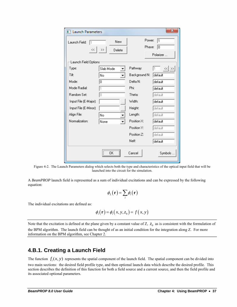
BeamPROP 8.0 User Guide Chapter 4: Using BeamPROP • 37
Figure 4-2. The Launch Parameters dialog which selects both the type and characteristics of the optical input field that will be
launched into the circuit for the simulation.
A BeamPROP launch field is represented as a sum of individual excitations and can be expressed by the following equation:
( ) ( )L ii
φ φ= ∑r r
The individual excitations are defined as:
( ) ( ) ( )0, , ,i i x y z f x yφ φ= =r
Note that the excitation is defined at the plane given by a constant value of Z, 0z as is consistent with the formulation of the BPM algorithm. The launch field can be thought of as an initial condition for the integration along Z. For more information on the BPM algorithm, see Chapter 2.
4.B.1. Creating a Launch Field The function ( , )if x y represents the spatial component of the launch field. The spatial component can be divided into two main sections: the desired field profile type, and then optional launch data which describe the desired profile. This section describes the definition of this function for both a field source and a current source, and then the field profile and its associated optional parameters.
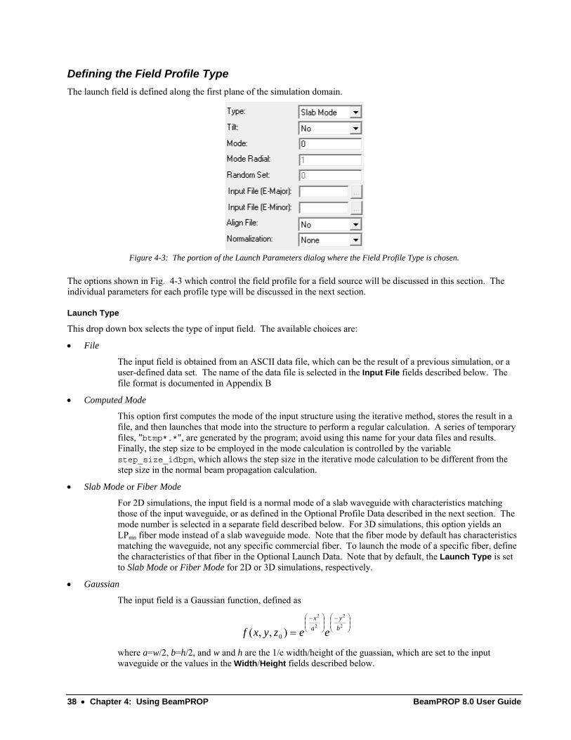
38 • Chapter 4: Using BeamPROP BeamPROP 8.0 User Guide
Defining the Field Profile Type The launch field is defined along the first plane of the simulation domain.
Figure 4-3: The portion of the Launch Parameters dialog where the Field Profile Type is chosen.
The options shown in Fig. 4-3 which control the field profile for a field source will be discussed in this section. The individual parameters for each profile type will be discussed in the next section.
Launch Type
This drop down box selects the type of input field. The available choices are:
• File
The input field is obtained from an ASCII data file, which can be the result of a previous simulation, or a user-defined data set. The name of the data file is selected in the Input File fields described below. The file format is documented in Appendix B
• Computed Mode
This option first computes the mode of the input structure using the iterative method, stores the result in a file, and then launches that mode into the structure to perform a regular calculation. A series of temporary files, "btmp*.*", are generated by the program; avoid using this name for your data files and results. Finally, the step size to be employed in the mode calculation is controlled by the variable step_size_idbpm, which allows the step size in the iterative mode calculation to be different from the step size in the normal beam propagation calculation.
• Slab Mode or Fiber Mode
For 2D simulations, the input field is a normal mode of a slab waveguide with characteristics matching those of the input waveguide, or as defined in the Optional Profile Data described in the next section. The mode number is selected in a separate field described below. For 3D simulations, this option yields an LPmn fiber mode instead of a slab waveguide mode. Note that the fiber mode by default has characteristics matching the waveguide, not any specific commercial fiber. To launch the mode of a specific fiber, define the characteristics of that fiber in the Optional Launch Data. Note that by default, the Launch Type is set to Slab Mode or Fiber Mode for 2D or 3D simulations, respectively.
• Gaussian
The input field is a Gaussian function, defined as
⎟⎟⎠
⎞⎜⎜⎝
⎛ −⎟⎟⎠
⎞⎜⎜⎝
⎛ −
=2
2
2
2
),,( 0by
ax
eezyxf
where a=w/2, b=h/2, and w and h are the 1/e width/height of the guassian, which are set to the input waveguide or the values in the Width/Height fields described below.

BeamPROP 8.0 User Guide Chapter 4: Using BeamPROP • 39
• Rectangle
The input field is a rectangular step function of unit value, and with a width and/or height of the input waveguide or the values in the Width/Height field described below.
• MultiMode
This is a specialized option useful for studying highly multimode waveguides. The input field is a superposition of all slab (2D) or fiber (3D) waveguide modes supported by the input waveguide, with equal power in each mode, and a random phase for each mode. The set of random phases is determined by a pseudo-random number generator, and does not vary from run to run; however, the user can select different sets of random phases through the Random Setfield described below. The set of modes that is launched may be controlled through the Mode field described below.
Tilt
This field selects whether or not the input optical field will be tilted so as to enter the circuit at an angle. By default, this option is set to No, and the optical field is launched along the Z axis with no angle. If this option is set to Yes, the optical wavefront is tilted to an angle equal to that of the input waveguide, unless it is overridden by the value in the Phi and Thetafields described below.
Mode
If the Launch Type is set to Slab Mode, this integer input field selects the mode number, counting from 0 which represents the fundamental mode and is the default. If the Launch Type is set to Multimode, this is a text input field which selects the mode set. The syntax is "low-high:step". The default is "*" which represents all modes. For example, "0-5" selects the first 6 modes, "*:2" selects all even modes, and "1-:2" selects all odd modes. In 3D, Slab Mode becomes Fiber Mode, and this field corresponds to the azimuthal mode number, m, of the corresponding LPmn fiber mode. Positive m corresponds to a cos(mϕφ)dependence and negative m corresponds to a sin(mϕφ) dependence.
Mode Radial
If the Launch Type is set to Fiber Mode, this integer input field selects the radial mode number, n, of the corresponding LPmn fiber mode.
Random Set
If the Launch Type is set to MultiMode, this integer input field selects the particular random set to be used for the random phases. The first set is numbered 0, and this is the default.
Input File (E-Major)
If the Launch Type is set to File, this text input field determines the file name for the input data corresponding to the major components of the electric field. The file format is described in Appendix B. The definition of the major component is discussed further in Section 7.A
Note that if a 2D data file is launched into a 3D simulation it is interpreted as a radial profile (as might be obtained via the Radial BPM option), and a corresponding 3D field distribution is automatically generated. The Mode field determines the azimuthal mode number as described above.
Input File (E-Minor)
If the Launch Type is set to File, this text input field determines the file name for the input data corresponding to the minor components of the electric field. The file format is described in Appendix B. The definition of the major component is discussed further in Section 7.A
Note that if a 2D data file is launched into a 3D simulation it is interpreted as a radial profile (as might be obtained via the Radial BPMoption), and a corresponding 3D field distribution is automatically generated. The Mode field determines the azimuthal mode number as described above.
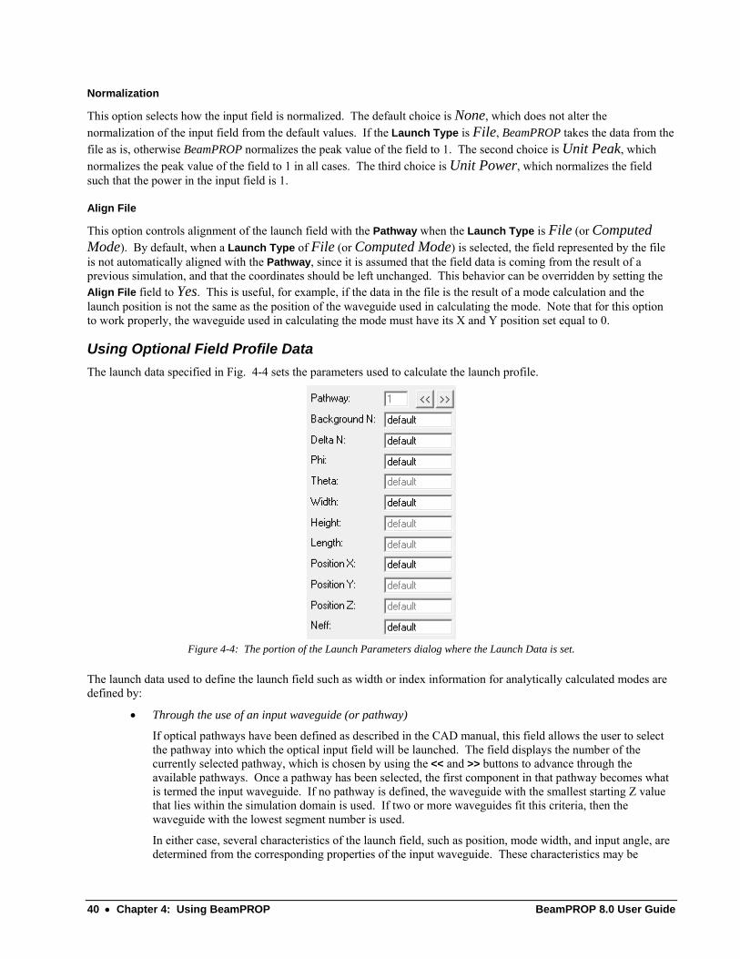
40 • Chapter 4: Using BeamPROP BeamPROP 8.0 User Guide
Normalization
This option selects how the input field is normalized. The default choice is None, which does not alter the normalization of the input field from the default values. If the Launch Type is File, BeamPROP takes the data from the file as is, otherwise BeamPROP normalizes the peak value of the field to 1. The second choice is Unit Peak, which normalizes the peak value of the field to 1 in all cases. The third choice is Unit Power, which normalizes the field such that the power in the input field is 1.
Align File
This option controls alignment of the launch field with the Pathway when the Launch Type is File (or Computed Mode). By default, when a Launch Type of File (or Computed Mode) is selected, the field represented by the file is not automatically aligned with the Pathway, since it is assumed that the field data is coming from the result of a previous simulation, and that the coordinates should be left unchanged. This behavior can be overridden by setting the Align File field to Yes. This is useful, for example, if the data in the file is the result of a mode calculation and the launch position is not the same as the position of the waveguide used in calculating the mode. Note that for this option to work properly, the waveguide used in calculating the mode must have its X and Y position set equal to 0.
Using Optional Field Profile Data The launch data specified in Fig. 4-4 sets the parameters used to calculate the launch profile.
Figure 4-4: The portion of the Launch Parameters dialog where the Launch Data is set.
The launch data used to define the launch field such as width or index information for analytically calculated modes are defined by:
• Through the use of an input waveguide (or pathway)
If optical pathways have been defined as described in the CAD manual, this field allows the user to select the pathway into which the optical input field will be launched. The field displays the number of the currently selected pathway, which is chosen by using the << and >> buttons to advance through the available pathways. Once a pathway has been selected, the first component in that pathway becomes what is termed the input waveguide. If no pathway is defined, the waveguide with the smallest starting Z value that lies within the simulation domain is used. If two or more waveguides fit this criteria, then the waveguide with the lowest segment number is used.
In either case, several characteristics of the launch field, such as position, mode width, and input angle, are determined from the corresponding properties of the input waveguide. These characteristics may be

BeamPROP 8.0 User Guide Chapter 4: Using BeamPROP • 41
overridden individually by entering explicit values into the Optional Launch Data portion of the dialog. Note that by default, pathway #1 will be selected. Also note that by default, when a Launch Type of File (or Computed Mode) is selected, the field represented by the file is not automatically aligned with the Pathway, but this behavior can be overridden by the Align File option. Refer to that option for further discussion.
• By directly setting the launch data
The relevant launch parameters can individually be specified so to override the default settings.
These fields control optional aspects of the launch field. For all these fields, the keyword default indicates that the default value will be used. To use a custom value, simply enter the desired value in the appropriate box.
Background N
This numeric input field selects the background index for the slab waveguide mode(s) to be launched. The default value corresponds to the background index of the circuit.
Delta N
This numeric input field selects the index difference for the slab waveguide mode(s) to be launched. The default value corresponds to the global index difference of the circuit.
Phi
This numeric input field selects the input angle in the XZ plane at which the input optical field is launched. The default value of this parameter is 0, and is measured from the Z axis. Note that this option must be used with the Tilt option described in the previous section.
Theta
This numeric input field selects the input angle in the YZ plane at which the input optical field is launched. The default value of this parameter is 0, and is measured from the Z axis. Note that this option must be used with the Tilt option described in the previous section.
Width
This numeric input field selects the lateral width along X of the optical input field to be launched. The default value corresponds to the global waveguide width.
Height
This numeric input field selects the vertical height along Y of the optical input field to be launched. The default value corresponds to the global waveguide height.
Length
This field is not used by BeamPROP.
Position X
This numeric input field selects the lateral (X) position at which the input optical field is launched. Note that if the Launch Type is set to File, the interpretation of this field assumes that the mode in the data file is centered at 0. In effect, the value in this field corresponds to an offset of the launch file data. Also note the comments under Pathway regarding the default value for this option.
Position Y
This numeric input field selects the vertical (Y) position at which the input optical field is launched (3D only). Note that if the Launch Type is set to File, the interpretation of the Position assumes that the mode in the data file is centered at
42 • Chapter 4: Using BeamPROP BeamPROP 8.0 User Guide
0. In effect, the value in this field corresponds to an offset of the launch file data. Also note the comments under Pathway regarding the default value for this option.
Position Z
This field is not used by BeamPROP.
Neff
This numeric input field selects the effective index corresponding to the propagation constant of the input light. This is required only when launching the field at an angle. The default corresponds to the actual propagation constant when the Launch Type is set to Slab Mode or Fiber Mode. When the Launch Type is File, and the data file is the result of a mode calculation, the default is to use the mode effective index stored in the file. Otherwise the default is the background index, and may need to be changed appropriately.
4.B.2. Polarization Manipulation BeamPROP allows for the inclusion of polarization effects in a simulation through the use of Vector BPM. The polarization of the launch field is defined within the context of the polarization of the simulation. and so the discussion on their use has been relegated to Section 7.A.
4.B.3. Launching Multiple Fields As noted above, the launch dialog shown in Fig. 4-4 allows the user to define multiple launch fields which can be linearly combined with different powers and phases. This multiple launch feature is controlled by several fields at the top of the dialog. The Launch Field setting indicates the number of the individual launch field currently being edited, and initially shows the value 1, corresponding to the default single launch field. To add one or more additional launch fields, click on the New button, and select the characteristic of that individual field in the remaining fields of the launch dialog as documented above. Use the << and >> buttons below the Launch Field field to switch between different individual fields to change their characteristics. To delete an individual launch field, click on the Delete button. Note that at least one launch field must be defined, so the program will not allow deletion of launch field #1 if it is the only launch field.
When performing a simulation, the individual launch fields are calculated and linearly combined to create the actual launch field that is used to initialize the simulation as described in Section 5.A. The coefficients used in performing the linear combination, the power and the phase, are determined from the Power and Phase fields in the upper right of the dialog respectively.
It is essential to note that when interpreting the power, the setting of the Normalization field plays a critical role. If two individual launch fields are combined without first being normalized to Unit Power, the values in the Power field will not in general reflect the actual relative power unless the individual fields have the same amplitude and shape.
4.C. Advanced & Bidirectional BPM Options The Advanced… and Bidirectional… button in the BPM Simulation Parameters dialog controls detailed aspects of the BPM algorithm and the bidirectional simulation feature. The Advanced BPM options are discussed in Section 7.B, and the Bidirectional BPM options in Section 7.C.
4.D. Display and Output Options The lower portion of the BPM Simulation Parameters dialog box defines the display and output of simulation results.
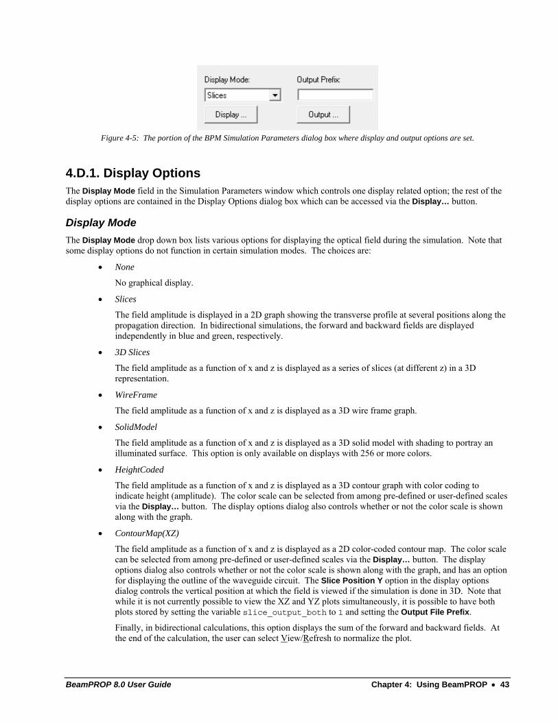
BeamPROP 8.0 User Guide Chapter 4: Using BeamPROP • 43
Figure 4-5: The portion of the BPM Simulation Parameters dialog box where display and output options are set.
4.D.1. Display Options The Display Mode field in the Simulation Parameters window which controls one display related option; the rest of the display options are contained in the Display Options dialog box which can be accessed via the Display… button.
Display Mode The Display Mode drop down box lists various options for displaying the optical field during the simulation. Note that some display options do not function in certain simulation modes. The choices are:
• None
No graphical display.
• Slices
The field amplitude is displayed in a 2D graph showing the transverse profile at several positions along the propagation direction. In bidirectional simulations, the forward and backward fields are displayed independently in blue and green, respectively.
• 3D Slices
The field amplitude as a function of x and z is displayed as a series of slices (at different z) in a 3D representation.
• WireFrame
The field amplitude as a function of x and z is displayed as a 3D wire frame graph.
• SolidModel
The field amplitude as a function of x and z is displayed as a 3D solid model with shading to portray an illuminated surface. This option is only available on displays with 256 or more colors.
• HeightCoded
The field amplitude as a function of x and z is displayed as a 3D contour graph with color coding to indicate height (amplitude). The color scale can be selected from among pre-defined or user-defined scales via the Display… button. The display options dialog also controls whether or not the color scale is shown along with the graph.
• ContourMap(XZ)
The field amplitude as a function of x and z is displayed as a 2D color-coded contour map. The color scale can be selected from among pre-defined or user-defined scales via the Display… button. The display options dialog also controls whether or not the color scale is shown along with the graph, and has an option for displaying the outline of the waveguide circuit. The Slice Position Y option in the display options dialog controls the vertical position at which the field is viewed if the simulation is done in 3D. Note that while it is not currently possible to view the XZ and YZ plots simultaneously, it is possible to have both plots stored by setting the variable slice_output_both to 1 and setting the Output File Prefix.
Finally, in bidirectional calculations, this option displays the sum of the forward and backward fields. At the end of the calculation, the user can select View/Refresh to normalize the plot.
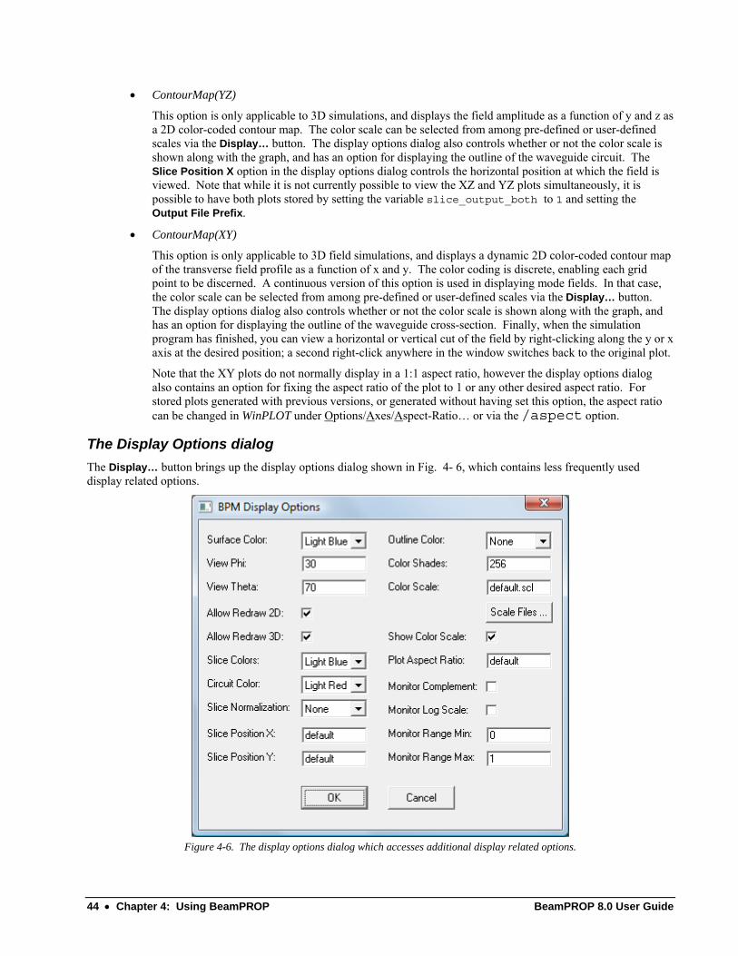
44 • Chapter 4: Using BeamPROP BeamPROP 8.0 User Guide
• ContourMap(YZ)
This option is only applicable to 3D simulations, and displays the field amplitude as a function of y and z as a 2D color-coded contour map. The color scale can be selected from among pre-defined or user-defined scales via the Display… button. The display options dialog also controls whether or not the color scale is shown along with the graph, and has an option for displaying the outline of the waveguide circuit. The Slice Position X option in the display options dialog controls the horizontal position at which the field is viewed. Note that while it is not currently possible to view the XZ and YZ plots simultaneously, it is possible to have both plots stored by setting the variable slice_output_both to 1 and setting the Output File Prefix.
• ContourMap(XY)
This option is only applicable to 3D field simulations, and displays a dynamic 2D color-coded contour map of the transverse field profile as a function of x and y. The color coding is discrete, enabling each grid point to be discerned. A continuous version of this option is used in displaying mode fields. In that case, the color scale can be selected from among pre-defined or user-defined scales via the Display… button. The display options dialog also controls whether or not the color scale is shown along with the graph, and has an option for displaying the outline of the waveguide cross-section. Finally, when the simulation program has finished, you can view a horizontal or vertical cut of the field by right-clicking along the y or x axis at the desired position; a second right-click anywhere in the window switches back to the original plot.
Note that the XY plots do not normally display in a 1:1 aspect ratio, however the display options dialog also contains an option for fixing the aspect ratio of the plot to 1 or any other desired aspect ratio. For stored plots generated with previous versions, or generated without having set this option, the aspect ratio can be changed in WinPLOT under Options/Axes/Aspect-Ratio… or via the /aspect option.
The Display Options dialog The Display… button brings up the display options dialog shown in Fig. 4- 6, which contains less frequently used display related options.
Figure 4-6. The display options dialog which accesses additional display related options.

BeamPROP 8.0 User Guide Chapter 4: Using BeamPROP • 45
Surface Color
This pulldown menu sets the surface color for plots produced when the Display Mode is set to SolidModel.
View Phi
This option sets the viewing angle Phi of the plots in the simulation window when the Display Mode is set to either SolidModel or HeightCoded
View Theta
This option sets the viewing angle Theta of the plots in the simulation window when the Display Mode is set to either SolidModel or HeightCoded.
Allow Redraw 2D
This option indicates that 2D plots displayed in the simulation window should be stored in memory so that the plots can be redrawn if needed. This option was used in early versions of BeamPROP to optimize memory usage on computer systems with minimal RAM. Today’s systems allow for this option to always be left on.
Allow Redraw 3D
This option indicates that 3D plots displayed in the simulation window should be stored in memory so that the plots can be redrawn if needed. This option was used in early versions of BeamPROP to optimize memory usage on computer systems with minimal RAM. Today’s systems allow for this option to always be left on. Slice Color
This field sets the color of the field slices displayed in the simulation window.
Circuit Color
This field sets the color of the circuit displayed behind the simulated fields in the simulation window.
Slice Normalization
This field has two options: None and Constant Peak. This choice indicates whether the slices should be normalized such that they all have the same peak or not.
Slice Position X
This field sets the slice position when the Display Mode in the Simulation Parameters window is set to ContourMap(YZ).
Slice Position Y
This field sets the slice position when the Display Mode in the Simulation Parameters window is set to ContourMap(XZ).
Outline Color
This pulldown menu sets the color of the circuit outline to be displayed over the simulated fields. By default, this option is set to None.
Color Shades
This option sets the number of color shades used to render plots in the simulation window.
Color Scale
This option sets the color scale used to render plots in the simulation window. Color Scale files can be chosen via the Color Scales… button.
Show Color Scale
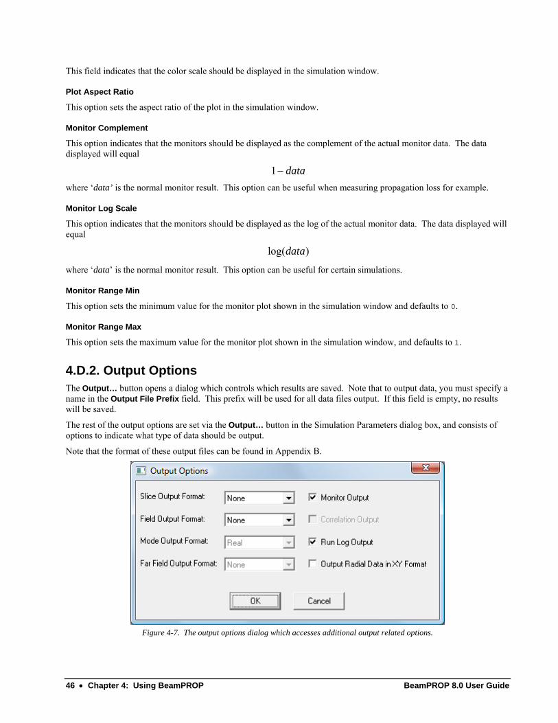
46 • Chapter 4: Using BeamPROP BeamPROP 8.0 User Guide
This field indicates that the color scale should be displayed in the simulation window.
Plot Aspect Ratio
This option sets the aspect ratio of the plot in the simulation window.
Monitor Complement
This option indicates that the monitors should be displayed as the complement of the actual monitor data. The data displayed will equal
1 data−
where ‘data’ is the normal monitor result. This option can be useful when measuring propagation loss for example.
Monitor Log Scale
This option indicates that the monitors should be displayed as the log of the actual monitor data. The data displayed will equal
log( )data
where ‘data’ is the normal monitor result. This option can be useful for certain simulations.
Monitor Range Min
This option sets the minimum value for the monitor plot shown in the simulation window and defaults to 0.
Monitor Range Max
This option sets the maximum value for the monitor plot shown in the simulation window, and defaults to 1.
4.D.2. Output Options The Output… button opens a dialog which controls which results are saved. Note that to output data, you must specify a name in the Output File Prefix field. This prefix will be used for all data files output. If this field is empty, no results will be saved.
The rest of the output options are set via the Output… button in the Simulation Parameters dialog box, and consists of options to indicate what type of data should be output.
Note that the format of these output files can be found in Appendix B.
Figure 4-7. The output options dialog which accesses additional output related options.

BeamPROP 8.0 User Guide Chapter 4: Using BeamPROP • 47
The following options are available:
Slice Output Format
This option sets the format for the field stored at each slice step. The default depends on the simulation options and display mode. Note that it can be useful to set this option to None to avoid large amounts of unwanted data to be saved, however certain graphs may not be generated. Slice data is saved in files with the names <prefix>.###, where ### is the number of the slice and <prefix> is the Output File Prefix selected. Additionally, the file <prefix>.pcs contains is a WinPLOT command file for graphing the standard display (slices and monitors).
Field Output Format
This option sets the format for saving the output field (field at final Z position). By default, it is set to None. The field is saved in a data file <prefix>.fld, with accompanying WinPLOT command file <prefix>.pfd where <prefix> is the Output File Prefix selected.
Mode Output Format
This option sets the format in which calculated modes, if any, are saved. By default it is set to Real. However if it is expected that the mode is complex, then a complex format such as Amp/Phase should be chosen. Mode files are saved in data files <prefix>.m## with WinPLOT command files <prefix>.p## where <prefix> is the Output File Prefix and ## is the mode number. Foe example, the file <prefix>.m00 corresponds to the fundamental mode.
Far Field Output
This option instructs the program to calculate both the amplitude and phase of the far field of either the output field or the mode field, depending on the type of simulation. Please note that the Field Output Format or Mode Output Format need to be set to a complex type (e.g. Amp/Phase) if the data they contain is expected to be complex (usually the case for field output, but not for mode output). By default far field output is set to No.
If an output prefix is specified when doing a mode calculation, this option will generate far field data files with the extension .f##, and corresponding graphs with the extension .pf#. For a propagation calculation, the user must also select an appropriate Field Output Format in the output options dialog (usually a complex format, such as Amp/Phase 2D or 3D as appropriate). Then, if an output prefix is specified when doing a propagation calculation, this option will generate far field data files with the extension .far, and corresponding graphs with the extension *.pfr. In both cases, the far field results are presented as intensity as a function of angle.
There are several additional options which control the far field calculations. First, the angular resolution can be controlled by setting the variable farfield_da to the required resolution in degrees. The resolution is normally set by the domain of the calculation, however this feature extends the domain during the far field calculation to attempt to achieve the requested resolution. Second, the far field is normally calculated by assuming the propagation is into air. To have the far field calculated assuming propagation into a different medium, set the farfield_index variable to the desired refractive index. Also, the variables farfield_axmin, farfieldax_max, farfield_axmin, and farfield_aymax allow user control over the angular range used in far-field plots.
Finally, we note that the far field calculations can also be performed on previously generated mode or field files via the command line utility bdutil noted in the RSoft CAD manual.
Monitor Output
This option instructs the program to save the monitor output if monitors have been defined. By default it is set to Yes. The raw monitor data is saved in a file <prefix>.mon, with a WinPLOT command file <prefix>.pmn where <prefix> is the Output File Prefix selected. See Chapter 5 for more information on the use of monitors.
Correlation Output
This option instructs the program to save the correlation function data from either a mode spectrum calculation, or a mode calculation using the correlation method. By default it is set to No. Note that this option is only provided for backward compatibility and may be removed in future versions since it is virtually never used.
Run Log Output

48 • Chapter 4: Using BeamPROP BeamPROP 8.0 User Guide
This option instructs the program to save a so-called run log, which is essentially a copy of the .ind file as it existed at the time of the simulation, with default simulation parameters replaced by the specific values used in the run. The run log is stored in the file prefix.run, and may be opened by clicking on the open file icon in the top toolbar, selecting Run Log Files in the Files of type field, and selecting the desired file. By default, this option is set to Yes.
Output Radial Data in XY Format
This option instructs the program to save output from a radial computation in XY format in addition to radial format.
BeamPROP 8.0 User Guide Chapter 5: Monitoring and Analysis of Simulation Results • 49
Chapter 5: Monitoring and Analysis of Simulation Results
The BeamPROP simulation program calculate the optical field as it propagates down the waveguide circuit. However, it is frequently useful to analyze the field in terms of certain physical quantities, such as the optical power in a particular region of the circuit. In order to meet this need, we introduce the concept of monitors in BeamPROP.
A BeamPROP monitor can produce various types of output:
• Field Power Output - These monitor types record the power in propagating fields either via an overlap integral or a power integral.
• Field Phase Output - These monitor types record the phase of a propagating field relative to a test field.
• Other Output - These monitor types record output such as spot size and 1/e width/height.
This chapter will discuss the steps for creating a monitor along with a detailed description of the usage of monitors.
5.A. Defining a Pathway The first step to create a time monitor is to define a pathway. This is done via the Edit Pathways button located in the left toolbar of the CAD interface. More details can be found in the RSoft CAD manual.
Note that pathways can include inactive components. An inactive component has its Profile Type set to Inactive as described in the RSoft CAD manual. This can be useful if it is necessary to monitor the power in a region which does not contain or is otherwise different from a true waveguide region.
5.B. Creating a Monitor To add a monitor to a pathway that has just been defined, click on the Monitors… button in the Pathway Edit Mode toolbar. If the pathway has previously been defined, enter Pathway Edit Mode by clicking on the pathways icon or choosing Edit/Tables/Edit-Pathways from the menu, select the desired pathway by clicking on the << or >> buttons, and then click on the Monitors… button. Alternatively, to access the monitors for all pathways, click on the monitors icon in the left toolbar (the power coupling graph), or select Edit/Tables/Edit-Monitors from the menu. In all cases, the monitors dialog appears as in Fig. 5-1.
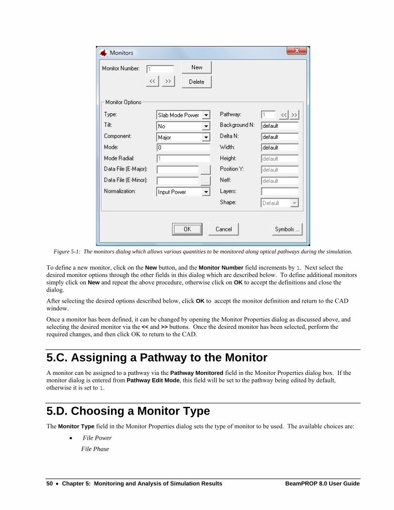
50 • Chapter 5: Monitoring and Analysis of Simulation Results BeamPROP 8.0 User Guide
Figure 5-1: The monitors dialog which allows various quantities to be monitored along optical pathways during the simulation.
To define a new monitor, click on the New button, and the Monitor Number field increments by 1. Next select the desired monitor options through the other fields in this dialog which are described below. To define additional monitors simply click on New and repeat the above procedure, otherwise click on OK to accept the definitions and close the dialog.
After selecting the desired options described below, click OK to accept the monitor definition and return to the CAD window.
Once a monitor has been defined, it can be changed by opening the Monitor Properties dialog as discussed above, and selecting the desired monitor via the << and >> buttons. Once the desired monitor has been selected, perform the required changes, and then click OK to return to the CAD.
5.C. Assigning a Pathway to the Monitor A monitor can be assigned to a pathway via the Pathway Monitored field in the Monitor Properties dialog box. If the monitor dialog is entered from Pathway Edit Mode, this field will be set to the pathway being edited by default, otherwise it is set to 1.
5.D. Choosing a Monitor Type The Monitor Type field in the Monitor Properties dialog sets the type of monitor to be used. The available choices are:
• File Power
File Phase

BeamPROP 8.0 User Guide Chapter 5: Monitoring and Analysis of Simulation Results • 51
These options compute the overlap integral between the calculated field at the current z position and the mode field specified by a data file, and use this result to determine the power in, or phase of, the specified mode, respectively. The data file in specified in the Data File(E-Major/E-Minor) fields described in Section 5.E. The phase is given in degrees from 0 to 360.
• Slab Mode Power or Fiber Mode Power
Slab Mode Phase or Fiber Mode Phase
These options compute the overlap integral between the calculated field at the current Z position and the local slab waveguide mode at that position, and use this result to determine the power in, or phase of, the specified mode, respectively. The mode number is selected in a separate field described below. The phase is given in degrees from 0 to 360. For 3D simulations, this option uses an LPmn fiber mode instead of a slab waveguide mode. Note that the fiber mode by default has characteristics matching the waveguide, not any specific commercial fiber. To monitor the mode of a specific fiber, define the characteristics of that fiber in the appropriate fields on the right side of the monitor dialog.
• Gaussian Power
Gaussian Phase
These options compute the overlap integral between the calculated field at the current Z position and a Gaussian mode field, and use this result to determine the power in, or phase of, the specified mode, respectively. The phase is given in degrees from 0 to 360.
• Launch Power
Launch Phase
These options compute the overlap integral between the calculated field at the current Z position and the input field for the simulation (i.e., the field defined in the launch parameters dialog), and use this result to determine the power in, or phase of, the specified mode, respectively. The phase is given in degrees from 0 to 360. Note that before doing the overlap, the input field is translated to align with the center of the pathway being monitored.
• Partial Power
This option computes the integral power in the calculated field at the current Z position over the waveguide cross section. The integral is computed between +/- (w/2 + f/γ), where w is the waveguide width, γ is a characteristic transverse decay constant for the waveguide, and f is a fractional parameter set by the internal variable monitor_decay_fraction, which defaults to 0. The characteristic decay length is determined from the highest supported slab waveguide mode, but is appropriately limited if that mode is nearly cutoff.
In 3D, the integration area depends in the type of waveguide structure. If the geometry of the waveguide in the pathway being monitored is a Fiber, the program will integrate over an ellipse (or circle if the width and height are equal). Otherwise, the program will integrate over a rectangle with width and height determined by the waveguide parameters or the Width/Height fields if they are other than default. The Monitors dialog also has a field for Shape, in which you can select Default, Rectangular, or Elliptical. (Default is Rectangular or Elliptical depending on the structure type as noted above).
• Total Power
This option computes the total power in the calculated optical field at the current Z position, and is therefore independent of pathway. In fact, pathways do not need to be defined in order to use this monitor, providing the Pathwayfield is set to 0.
• Effective Index
This is an advanced feature which should only be used by experienced users.
This option computes the mode effective index of the calculated optical field at the current Z, and must be used in conjunction with an iterative mode calculation. This option is useful when doing a parameter scan to obtain a plot of the effective index versus some parameter. Note this option is independent of the pathway. Also note that for most situations the use this option has been superceded by the fact that when
52 • Chapter 5: Monitoring and Analysis of Simulation Results BeamPROP 8.0 User Guide
doing a mode calculation inside parameter scan, the mode effective index versus the scanned variables is now automatically stored in the .nes/.pne data and plot files, respectively.
• Field 1/e Width
Field 1/e Height
These options compute the 1/e width and height of the calculated optical field at the current Z position. Note these options are independent of the pathway.
Note for Phase Monitors The value returned by the phase monitor is the phase of the slowly varying field ( ), ,u x y z described in Section 2.B.1.
In order to derive the phase of the physical field ( ), ,x y zφ , we can use the following relation introduced in Section 2.B.1
( ) ( ), , , , i k zx y z u x y z eφ =
The phase of the physical field is therefore equal to
180Monitor Result kzπ
+
The value returned by the phase monitor is normalized to the kbar value, and equals
( )zk k z− ⋅
5.E. Monitor Options Once the Monitor Type has been chosen, the relevant monitor options can be set in the Monitor Properties dialog box.
Tilt
If the Monitor Type involves an overlap integral, this field selects whether or not the local monitor field will be tilted to the local waveguide angle before calculating the integral.
Component
This option selects which field components are used in calculating the monitor value, and is relevant for full-vector calculations and/or bidirectional calculations. With respect to full-vector calculations, the choices Major, Minor, and Both correspond to the stated components of the field. With respect to bidirectional calculations, the options Major, Minor, and Both refer to the corresponding component of the forward field, while Major - Backward, Minor - Backward, and Both - Backward refer to the corresponding component of the backward field.
Mode
If the Monitor Type is set to Slab Mode Power or Phase, this integer input field selects the mode number, counting from 0 which represents the fundamental mode and is the default. Note that specifying a "*" in this field requests that all supported modes be included in the power calculation. In 3D, Slab Mode becomes Fiber Mode, and this field corresponds to the azimuthal mode number, m, of the corresponding LPmn fiber mode. Positive m corresponds to a cos(mϕ) dependence and negative m corresponds to a sin(mϕ) dependence.
Mode Radial
If the Monitor Type is set to Fiber Mode, this integer input field selects the radial mode number, n, of the corresponding LPmn fiber mode.

BeamPROP 8.0 User Guide Chapter 5: Monitoring and Analysis of Simulation Results • 53
Data File (E-Major/E-Minor)
If the Monitor Type is set to File Power or File Phase, these text input fields determine the file name(s) for the input data corresponding to the major and minor components of the electric field, respectively. The file format is described in Appendix B. The file is assumed to be centered at x = 0 and y = waveguide center. The Position Y field can be used to offset the field in the vertical direction if necessary. Note that if a 2D data file is specified in a 3D simulation, it is interpreted as a radial profile (as might be obtained via the Radial BPM option for example), and a corresponding 3D field distribution is automatically generated. The Mode field determines the azimuthal mode number as described above.
Normalization
This option selects how the monitor values are normalized. The default choice is Input Power, which normalizes power monitors to the total power in the input field. Another choice is Local Power, which normalizes power monitors to the total power in the calculated field at the current Z position. This is useful when trying to obtain the fraction of the field inside a region, where the total power may be decaying or has otherwise changed from the input power. An example would be in trying to obtain the local confinement factor of a tapered structure.
Background N
This numeric input field selects the background index for the slab or fiber mode to be used as the monitor field. The default is to use the background index of the circuit, and is specified by the keyword default.
Delta N
This numeric input field selects the index difference for the slab or fiber mode to be used as the monitor field. The default is to use the local waveguide index difference, and is specified by the keyword default.
Width
This numeric input field selects the lateral width of the monitor field (or integration area for Partial Power). The default is to use the local waveguide width, and is specified by the keyword default.
Height
This numeric input field selects the vertical height of the monitor field (or integration area for Partial Power). The default is to use the local waveguide height, and is specified by the keyword default.
Position Y
This numeric input field selects the vertical position of the monitor field. The default is at the center of the local waveguide structure, and is specified by the keyword default. Note that while there is currently no option to alter the lateral position of the monitor field (which is always centered on the pathway), it is usually possible to achieve the desired effect by defining an inactive series of waveguides, and a corresponding pathway, along the desired path to be monitored. To make a waveguide inactive, set its Profile Type to Inactive.
Neff
This numeric input field selects the effective index corresponding to the propagation constant of the monitor field. This is required only when monitoring the field at an angle. The default (specified by the keyword default) corresponds to the actual propagation constant when the Monitor Type is set to Slabor Fiber Mode (Power or Phase). When the Monitor Type is File (Power or Phase), and the data file is the result of a mode calculation, the default is to use the mode effective index stored in the file. Otherwise the default is the background index, and may need to be changed appropriately.
Layers
This option is relevant for Multilayer structures, and must be used with a Monitor Type of Partial Power. It allows you to select a range of layers to be included in the calculation. The range is specified as either a single layer number, or a starting layer number, a hyphen, and an ending layer number (e.g. “2-5”). This option, in conjunction with Normalization, is useful for determining confinement factors.

54 • Chapter 5: Monitoring and Analysis of Simulation Results BeamPROP 8.0 User Guide
Shape
This option selects the shape of the domain for a Partial Power monitor. Its default behavior is Rectangular for channel structure types, and Elliptical for fiber structure types.

BeamPROP 8.0 User Guide Chapter 6: Mode Solving • 55
Chapter 6: Mode Solving
BeamPROP includes two fully functional mode solvers: the iterative method and the correlation method. Both of these methods are based on the Beam Propagation Method, or BPM.
The mode solvers can be to solve for the propagating modes of a structure with an arbitrary 2D or 3D index cross section. The formulation and usage of the mode solvers will be discussed.
6.A. Background Both mode solvers in BeamPROP are based on the BPM algorithm used in the BeamPROP simulation tool. The mathematical background for these mode solvers can be found in Section 2.B.7.
6.B. Mode Solving Overview Mode solving can be thought of as a six step process. These steps are:
Step 1: Create the index structure in the RSoft CAD tool. In order to solve for the mode of a structure, the structure has to be created. The structure should be uniform in Z, and have the desired index profile. Be sure to use the Compute Index Profile option to check that the profile is indeed correct.
Step 2: Choose the appropriate mode solver and related options. As discussed above, BeamPROP contains two mode solvers. The one you choose depends on the type of modes you want to find. Generally:
• The iterative method is the default choice and is recommended for most standard waveguide problems.
• The correlation method can have advantages for problems such as antiguiding, leaky, lossy, or radiating modes, or when large numbers of modes need to be calculated.
The desired mode solver, along with several related options, can be found in the Mode Calculation Options dialog shown in Fig. 6-1 which can be opened by clicking the Mode Options… button in the Compute Mode dialog.
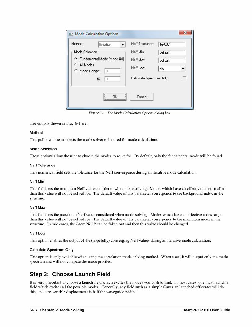
56 • Chapter 6: Mode Solving BeamPROP 8.0 User Guide
Figure 6-1. The Mode Calculation Options dialog box.
The options shown in Fig. 6-1 are:
Method
This pulldown menu selects the mode solver to be used for mode calculations.
Mode Selection
These options allow the user to choose the modes to solve for. By default, only the fundamental mode will be found.
Neff Tolerance
This numerical field sets the tolerance for the Neff convergence during an iterative mode calculation.
Neff Min
This field sets the minimum Neff value considered when mode solving. Modes which have an effective index smaller than this value will not be solved for. The default value of this parameter corresponds to the background index in the structure.
Neff Max
This field sets the maximum Neff value considered when mode solving. Modes which have an effective index larger than this value will not be solved for. The default value of this parameter corresponds to the maximum index in the structure. In rare cases, the BeamPROP can be faked out and then this value should be changed.
Neff Log
This option enables the output of the (hopefully) converging Neff values during an iterative mode calculation.
Calculate Spectrum Only
This option is only available when using the correlation mode solving method. When used, it will output only the mode spectrum and will not compute the mode profiles.
Step 3: Choose Launch Field It is very important to choose a launch field which excites the modes you wish to find. In most cases, one must launch a field which excites all the possible modes. Generally, any field such as a simple Gaussian launched off center will do this, and a reasonable displacement is half the waveguide width.
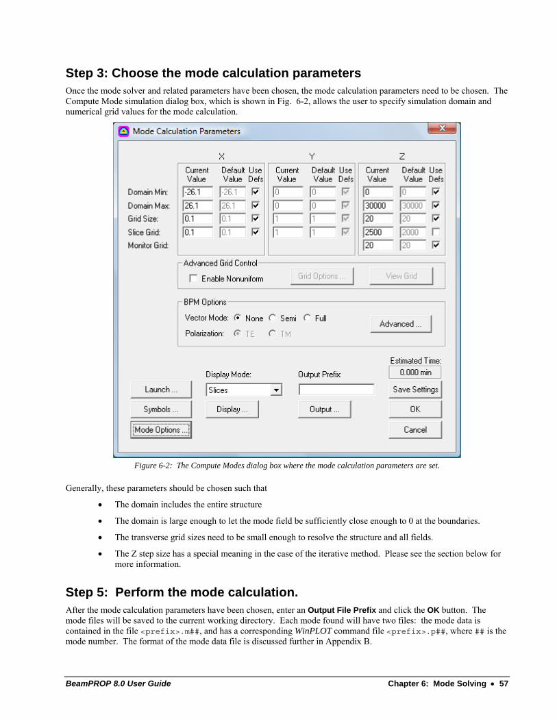
BeamPROP 8.0 User Guide Chapter 6: Mode Solving • 57
Step 3: Choose the mode calculation parameters Once the mode solver and related parameters have been chosen, the mode calculation parameters need to be chosen. The Compute Mode simulation dialog box, which is shown in Fig. 6-2, allows the user to specify simulation domain and numerical grid values for the mode calculation.
Figure 6-2: The Compute Modes dialog box where the mode calculation parameters are set.
Generally, these parameters should be chosen such that
• The domain includes the entire structure
• The domain is large enough to let the mode field be sufficiently close enough to 0 at the boundaries.
• The transverse grid sizes need to be small enough to resolve the structure and all fields.
• The Z step size has a special meaning in the case of the iterative method. Please see the section below for more information.
Step 5: Perform the mode calculation. After the mode calculation parameters have been chosen, enter an Output File Prefix and click the OK button. The mode files will be saved to the current working directory. Each mode found will have two files: the mode data is contained in the file <prefix>.m##, and has a corresponding WinPLOT command file <prefix>.p##, where ## is the mode number. The format of the mode data file is discussed further in Appendix B.

58 • Chapter 6: Mode Solving BeamPROP 8.0 User Guide
In addition, the correlation method has several other output files which are discussed below.
6.C. Using the Iterative Method This section describes how to obtain modal characteristics using the iterative function method as described in [1]. The iterative method is an alternative and significantly faster approach (in general) for obtaining the field shape and propagation constant for the fundamental mode, as well as higher order modes, than the correlation method. The computations are performed using the so-called imaginary distance beam propagation method as described in [2,3].
The length of the Z-independent index structure can be made arbitrary, provided it is at least about 1-10 mm long, since the method is iterative and will automatically stop if it converges before the specified length. If it fails to converge before the specified length a warning is issued, and the length should be increased. This warning can be disabled by setting the variable idbpm_convergence_warning to 0, although it is still noted in the log file, log.txt.
6.C.1. Computing Modes To perform the calculation, either click on the mode field icon in the left toolbar to solve for the fundamental mode, or select Run/Compute-Fundamental-Mode from the menu. Note that the mode files will only be saved if an Output File Prefix is specified. Additionally, the lowest order mode found will be displayed on-screen when the simulation has completed. To access other modes, use the View Graphs button.
The effective index of the modes can be found in the file <prefix>.nef file. See Appendix B for the format of this file.
6.C.2. Additional Notes There are several considerations that must be taken into account when computing mode eigenvalues and eigenfunctions via the iterative method.
The Launch Field One must launch a field which excites all the possible modes. Generally, any field such as a simple guassian launched off center will do this, and a reasonable displacement is half the waveguide width.
The Step Size The recommended step size is different than for the case of a BPM standard field propagation. Usually this recommendation is the maximum stable step size which yields the most rapid convergence. However, too large a step size can sometimes cause the iteration to converge to an undesired or unphysical mode. These modes are usually distinguished by unphysical discontinuities in the field pattern, best observed in scalar mode where all fields are continuous. If this occurs, reduce the step size by factors of about two until convergence to the desired mode is obtained. Note that reducing the step size further will provide no benefit in accuracy, only slower convergence. Since the ideal step size for the iterative mode calculation is usually different from that for BPM propagation, the program maintains both settings for convenience.
The default step size is determined from a theoretical ideal, and multiplied by a safety factor which should normally be less than one. This safety factor is controlled by the variable step_size_idbpm_factor which defaults to 0.5. The advantage of this over simply setting the step size for the iterative method is that when using the automatic setting of the step size, it will scale properly as other variables, such as the index, change.
Convergence Tolerance The default convergence criterion is that the normalized effective index change by less than 10-7 between iterations. The Neff Tolerance field in the Mode Calculation Options dialog controls this parameter. Note that in some cases the effective index can oscillate and fail to converge. If this occurs, set the tolerance to a less stringent value, such as 10-6.
BeamPROP 8.0 User Guide Chapter 6: Mode Solving • 59
In other cases, the effective index will converge, but the mode pattern may not. If this appears to be the case, set the tolerance to a more stringent value, such as 10-8.
6.D. Using the Correlation Method This section describes how to obtain modal characteristics using the correlation function method as described in [1]. Two example files, MODES2D.IND and MODES3D.IND, have been defined to illustrate this feature.
The correlation method uses two full BPM propagations in order to solve for the modes of a structure. In the first propagation, the mode spectrum is found. From this spectrum, the eigenvalues, or neff values for each mode are found. In the second simulation, the mode profiles, or eigenfunctions, are found.
First we will discuss the calculation of the mode spectrum, and then the calculation of the mode field profiles.
6.D.1. Computing only the Mode Spectrum To compute only the mode spectrum, select the appropriate option in the Mode Options dialog.
This step is automatically done if calculating the mode profiles as discussed in the next section.
If Compute Mode Spectrum is chosen, BeamPROP will first perform a field computation and display the results as usual. At the end of the field computation the field display will clear and the mode spectrum will be graphed. The mode spectrum represents the FFT of the correlation function, as described in the above reference. It exhibits one or more peaks at the frequencies of the guided modes, each with a height equal to the fraction of power in the input field contained in that mode.
The frequency axis in this graph is defined by the mode effective index minus the reference index, or
0
bareff bar
kn nk
β −− =
If an output prefix is specified the results will be saved in the following files: Filename Description
<prefix>.cor The correlation function. This file is not saved by default.
<prefix>.fft The FFT of the correlation function
<prefix>.pft An WinPLOT command file for the mode spectrum graph
<prefix>.nef A list of the mode frequencies that were found.
See Appendix B for the format of these files. Note that the mode spectrum contains the uncorrected propagation constants as discussed in the next section.
When performing a mode spectrum calculation inside parameter scan, as described in the CAD manual, the mode effective index versus the scanned variables is automatically stored in the <prefix>.nes and <prefix>.pne data and WinPLOT plot files, respectively.
6.D.2. Computing the Mode Profiles and Propagation Constants If Compute Mode is chosen, BeamPROP first performs a mode spectrum calculation as described above. At the end of the first field computation the mode spectrum display flashes on screen, and a second field computation begins. At the end of the second field computation the desired mode will be graphed. For a 2D simulation the real and imaginary parts of the mode will be displayed as a line plot, and for a 3D simulation the amplitude will be displayed as a contour plot. The user must specify which modes should be solved for via the options described in Section 6.B.
60 • Chapter 6: Mode Solving BeamPROP 8.0 User Guide
The mode files will only be saved if an Output File Prefix is specified. Additionally, the lowest order mode found will be displayed on-screen when the simulation has completed. To access other modes, use the View Graphs button.
Corrections Used To Calculate Effective Indices As discussed in Section 2.B.7, two corrections can be applied which results in more accurate effective index values. The first correction accounts for the fact that the paraxial equation was solved, and not the exact Helmholtz equation.
Another correction uses the mode profiles to calculate the propagation constants by substituting the mode profiles into the wave equation. This method not only results in a more accurate effective index, but also allows the imaginary part of the propagation constant to be found. This method is controlled by the variable neff_method, and is enabled by default.
The effective index values displayed in any output files such as the .nef file or any mode files (.m##) or plots (.p##) uses the corrected value, and not the value in the mode spectrum. If needed, the three real propagation constant values (uncorrected, first correction only, first and second correction), and the imaginary value can be found in the .mds file described in Appendix B.
The Imaginary Propagation Constant If the variable neff_method is enabled, which it is by default, the program will save the imaginary part of the effective index. This output can be disabled via the variable neff_method. Note, however, that the first correction to the real effective index described above is still taken.
The imaginary part of the propagation constant, ( )Im effn represents the propagation loss of the mode. This parameters
is expressed as:
( )Im4effn γλπ
=
where λ is the wavelength and γ is the usual exponential loss coefficient defined such that the power decays as ze γ− , and is given in units of μm-1.
6.D.3. Additional Notes There are several considerations that must be taken into account when computing mode eigenvalues and eigenfunctions via the correlation method.
The Launch Field One must launch a field which excites all the possible modes. Generally, any field such as a simple guassian launched off center will do this, and a reasonable displacement is half the waveguide width.
FFT Related Considerations Second, since the computation of the mode frequencies is performed using an FFT of the correlation function, the accuracy and bandwidth of the spectrum are determined by standard Fourier sampling principles. Namely, the narrowness of the peaks, which determines how well closely spaced peaks can be resolved, is determined by the propagation length - the longer the propagation the better the resolution. Furthermore, the range of frequencies is determined by the sampling period - the shorter the sampling period the wider the range of frequencies. Note that the sampling period is not the same as the computational step size, but is equal to the monitor step size. Thus a fine computational step size may be employed, but the monitor step size can be adjusted to reduce the range of frequencies (and the memory and time requirements for the FFT). This is important since the bound eigenmodes are limited in bandwidth (i.e. nmin<neff<nmax), thus there is no need for the frequency range to be infinitely large.

BeamPROP 8.0 User Guide Chapter 6: Mode Solving • 61
Finding Eigenvalues from the Spectrum Note that while the search algorithm limits the mode peaks to the frequency range specified by the Neff Min and Neff Max values, care must be taken to experiment with the propagation length and numerical parameters to ensure that spurious modes are not determined. The search algorithm enumerates peaks above a certain fraction of the maximum peak height. This fraction defaults to 0.01, and can be controlled by the symbol table variable mode_threshold.
6.E. Additional Comments This section contains additional comments about the mode solvers included with BeamPROP.
6.E.1. Finding Asymmetric Higher Order Modes with the Iterative Method There is an alternative method to compute the first order asymmetric mode of a structure symmetric about x=0. This mode has a null at x=0, and the field for x>=0 can be considered the fundamental mode of the structure in the corresponding half plane which satisfies Dirichlet boundary conditions at the left boundary. Since the imaginary distance BPM technique finds the fundamental mode of a structure consistent with the applied boundary conditions, we can obtain the desired mode by
• Restrict the domain of the computation to x>=0 by setting the X Domain Min field in the simulation parameters dialog to 0.
• Set the boundary condition at the left boundary to Dirichlet by setting the variable bc_type_left to BC_DIRICHLET.
After making these settings, selecting Run/Compute-Fundamental-Mode will compute the propagation constant and positive half of the field for the desired asymmetric mode.
6.E.2. Calculating Modes from the Command Line The mode solving features can be accessed from the command line using the symbol table variables mode_method, mode_spectrum and mode_set. The mode_method variable sets the mode solver to be used. A value of 0 corresponds to the correlation method, and 1 corresponds to the iterative method. The mode_spectrum variable should be set to 1 to compute the mode spectrum instead of the optical field. The mode_set variable can be a single integer to select one mode, or a range specification (low-high) to select several modes, or an asterisk (*) to select all modes.
6.E.3. Saving the Magnetic Field The H field can also be saved when performing a mode calculation. To do this, set the variable hfield_output = 1. This will derive and save the H field corresponding to the E field that is determined in the mode calculation. The H field will be saved in data files with the extension .mh# (or .nh# for the minor component).
6.E.4. Parameter Scans When performing a mode calculation inside parameter scan, the mode effective index versus the scanned variables is automatically stored in the data file <prefix>.nes and the WinPLOT plot file <prefix>.pne. This output is controlled by the variable neff_scan_output. Its possible values are: Value Description
0 Disables any effective index output during a scan.
1 Saves the real part of the effective index to the .nes file. This is the default value for this parameter.
2 Saves both the real and imaginary parts of the effective index to the .nes file..

62 • Chapter 6: Mode Solving BeamPROP 8.0 User Guide
Please see the CAD manual for more information about parameter scans.
6.E.5. Setting the Mode Calculation Length By default, the mode computation will be performed from the Domain Min value in Z until the Domain Max is reached or, for the iterative method only, when a converged result is found. This behavior can be changed via the variable mode_length. When this variable is defined, any mode computation will start at the Domain Min and continue for a length equal to mode_length, or for the iterative method only, when a converged result is found.
This option does not require the structure to be defined over the entire length since the program will use the structure at Z Domain Min to find the mode. This variable can have several special values: Value Description
undefined or -1 The values given in Domain Min and Domain Max determine the length.
default The program will automatically determine a length. Currently, this length is set to 1000 propagation steps for the iterative method. For the correlation method, the variable neff_tol_cor is used to set a desired tolerance for the effective indices. The default value for this parameters is 1e-4. Based on this variable, the a default length will be chosen which attempt to satisfy this tolerance. Note that this is only one factor determining final accuracy - step size and grid size must be considered as well.
any other value This sets the mode calculation length to the value given in µm.
Also, when the correlation method is used and mode_length is set either explicitly or to default, the length will be rounded to the nearest power of 2 multiple of the step size, as required by the method.
6.F. References [1] M.D. Feit and J.A. Fleck, “Computation of Mode Properties in Optical Fiber Waveguides by a Propagating Beam Method,” Applied Optics, 19, 1154 (1980)
[2] D. Yevick and B. Hermansson, “New formulations for the Beam Propagation Method: Application to Rib Waveguides,” J. Quantum Electronics, 25, 221 (1989)
[3] D. Yevick and Witold Bardyszewski, “Correspondence of Variational Finite-Difference (Relaxation) and Imaginary-Distance Propagation Methods for Modal Analysis,” Optical Letters, 17, 328 (1992)
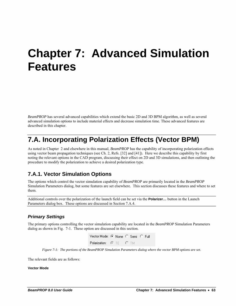
BeamPROP 8.0 User Guide Chapter 7: Advanced Simulation Features • 63
Chapter 7: Advanced Simulation Features
BeamPROP has several advanced capabilities which extend the basic 2D and 3D BPM algorithm, as well as several advanced simulation options to include material effects and decrease simulation time. These advanced features are described in this chapter.
7.A. Incorporating Polarization Effects (Vector BPM) As noted in Chapter 2 and elsewhere in this manual, BeamPROP has the capability of incorporating polarization effects using vector beam propagation techniques (see Ch. 2, Refs. [32] and [41]). Here we describe this capability by first noting the relevant options in the CAD program, discussing their effect on 2D and 3D simulations, and then outlining the procedure to modify the polarization to achieve a desired polarization type.
7.A.1. Vector Simulation Options The options which control the vector simulation capability of BeamPROP are primarily located in the BeamPROP Simulation Parameters dialog, but some features are set elsewhere. This section discusses these features and where to set them.
Additional controls over the polarization of the launch field can be set via the Polarizer… button in the Launch Parameters dialog box. These options are discussed in Section 7.A.4.
Primary Settings The primary options controlling the vector simulation capability are located in the BeamPROP Simulation Parameters dialog as shown in Fig. 7-1. These option are discussed in this section.
Figure 7-1: The portions of the BeamPROP Simulation Parameters dialog where the vector BPM options are set.
The relevant fields are as follows:
Vector Mode
64 • Chapter 7: Advanced Simulation Features BeamPROP 8.0 User Guide
This radio button field has three options: None, Semi, and Full. When this field is set to None, BeamPROP uses the scalar BPM as described in Chapter 2. The Semi and Full options correspond to the so-called semi-vectorial and full-vectorial methods commonly noted in the literature (see, for example, Ch. 2, Ref. [32]). The precise meaning of these options is described in the following sections.
Polarization
This radio button field has two options: TE and TM. These describe the polarization of the optical field (or predominant polarization in the case of full-vector where the fields are hybrid). The precise meaning of these options is described in the following sections. Note that depending on the Vector Mode and other settings, the Polarization options may be grayed out as appropriate if they are not applicable or not available.
Other Settings In addition to the polarization options in the startup/global settings dialogs, BeamPROP has several options which control advanced aspects of the methods used for vector BPM.
• The software has the option to use a formulation based on the magnetic field rather than the electric field. This option is enabled through the Formulation option in the Advanced Parameters dialog. See Section 7.B for more details.
• Anisotropic Calculations can be enabled via a checkbox in the Advanced Parameters dialog which can be opened by clicking the Advanced… button in the BeamPROP Simulation Parameters dialog. See Section 7.B for details.
• The Vector Conserve option can help conserve power in some cases. See Section 7.B for details.
• As stated earlier, the polarization field as defined above can be manipulated to achieve a custom polarization. This can be accomplished for each launch field separately via the Polarizer… button in the Launch Parameters dialog.
7.A.2. 2D Vector BPM This section covers the geometry, orientation, and definition of the various Vector Mode options for 2D vector BPM.
Geometry and Orientation The index gradient is along x, and the structure is considered infinite and uniform along y. As always, the primary direction of propagation is along z. These conventions, along with Maxwell's equations, imply that TE polarization is along y and TM polarization is along x. This determines the meaning of the Polarization field.
Vector Modes The nature of Maxwell's equations for 2D geometry is such that:
• A scalar calculation is equivalent to a TE calculation.
• There is no difference between semi-vectorial and full-vectorial calculations.
Thus, the vector modes are as follows: Vector Mode Description
None A TE calculation is performed independent of the Polarization Setting
Semi or Full The Polarization field determines the polarization used in the beam propagation calculation. A semi-vectorial simulation simulates each polarization separately, while a full-vectorial simulation simulates both polarizations and the coupling between them.

BeamPROP 8.0 User Guide Chapter 7: Advanced Simulation Features • 65
7.A.3. 3D Vector BPM This section covers the geometry, orientation, and definition of the various Vector Mode options for 3D vector BPM.
Geometry and Orientation The index gradient is along both x and y, thus no particular orientation is necessarily selected out. However, in the case of multilayer structures the primary index gradient is along y. As always, the primary direction of propagation is along z. These conventions, along with Maxwell's equations, imply that quasi-TE polarization is along x and quasi-TM polarization is along y. This determines the meaning of the Polarization field.
Vector Modes The nature of Maxwell's equations for 3D geometry is such that:
• A scalar calculation is not equivalent to either polarization. However, in the case of a Fiber, it is equivalent to the so-called LP modes.
• A pure TE or TM wave does not exist, however for most structures quasi-TE and quasi-TM waves exist in which the most of the field energy is in one polarization (the major component) and only a small fraction (less than one percent) is in the other polarization (the minor component).
The vector modes are as follows: Vector Mode Description
None A scalar calculation is performed which is an approximation that is accurate when the index difference is small.
Semi A semi-vectorial calculation is performed in which the minor component of the field is neglected (set to zero), and polarization is partially taken into account by employing the proper field equations for the major component. This approximation is very accurate in many cases since, as noted above, the minor component of the field is frequently negligible. This option can discriminate between quasi-TE and quasi-TM fields and can be used to determine differences in field shapes and propagation constants.
Full A full-vectorial calculation is performed in which both components of the field, and the coupling between them, are taken into account. Generally this option only needs to be employed if it is desired to estimate the amplitude of the minor field component or the coupling between polarizations. Note that this option is significantly slower than the other options. In addition, it is not unconditionally stable with respect to grid size, and the Scheme Parameter in the advanced numerical parameters dialog may need to be adjusted to ensure stability (see Ch. 2, Ref. [32] for the definition of the scheme parameter).
7.A.4. Manipulating the Polarization of the Launch Field As stated earlier, the polarization of the launch field is defined within the context of the default polarization for the simulation. These defaults will first be discussed, followed by several options which allow these defaults to be changed.
These options are only valid when Vector Mode is set to Full. For semi-vectorial simulations, the polarization of the launch is set equal to the Polarization set in the Global Settings, and for scalar simulations, the polarization does not need to be defined.
Assuming a Waveguide Dimension and Polarization option in the Global Settings dialog have been chosen, the default launch polarization can be manipulated. There are two polarization manipulation options:
• Transformer Mode
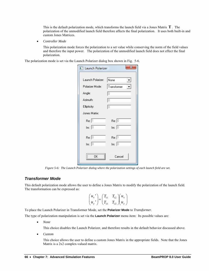
66 • Chapter 7: Advanced Simulation Features BeamPROP 8.0 User Guide
This is the default polarization mode, which transforms the launch field via a Jones Matrix Τ . The polarization of the unmodified launch field therefore affects the final polarization. It uses both built-in and custom Jones Matrices.
• Controller Mode
This polarization mode forces the polarization to a set value while conserving the norm of the field values and therefore the input power. The polarization of the unmodified launch field does not effect the final polarization.
The polarization mode is set via the Launch Polarizer dialog box shown in Fig. 5-6.
Figure 5-6: The Launch Polarizer dialog where the polarization settings of each launch field are set.
Transformer Mode This default polarization mode allows the user to define a Jones Matrix to modify the polarization of the launch field. The transformation can be expressed as:
11 12
21 22
''
x x
y y
u uT Tu uT T
⎛ ⎞ ⎛ ⎞⎛ ⎞=⎜ ⎟ ⎜ ⎟⎜ ⎟
⎝ ⎠⎝ ⎠ ⎝ ⎠
To place the Launch Polarizer in Transformer Mode, set the Polarizer Mode to Transformer.
The type of polarization manipulation is set via the Launch Polarizer menu item: Its possible values are:
• None
This choice disables the Launch Polarizer, and therefore results in the default behavior discussed above.
• Custom
This choice allows the user to define a custom Jones Matrix in the appropriate fields. Note that the Jones Matrix is a 2x2 complex-valued matrix.

BeamPROP 8.0 User Guide Chapter 7: Advanced Simulation Features • 67
• Linear
This choice enables a linear polarization at a specified angle. The Jones Matrix is therefore real, and can be expressed as
2
2
cos cos sincos sin sin
φ φ φφ φ φ
⎛ ⎞= ⎜ ⎟
⎝ ⎠T
where φ is the angle specified in the Angle field.
• Circular Left
This choice enables a left circularly polarized field. The Jones Matrix is therefore
11
12i
i−⎛ ⎞
= ⎜ ⎟⎝ ⎠
T
• Circular Right
This choice enables a right circularly polarized field. The Jones Matrix is therefore
11
12i
i⎛ ⎞
= ⎜ ⎟−⎝ ⎠T
• Rotation
This choice performs a simple rotation based on the value specified in the Angle field. The Jones Matrix is therefore real valued and can be expressed as:
cos sinsin cos
φ φφ φ
⎛ ⎞= ⎜ ⎟−⎝ ⎠
T
Controller Mode This polarization mode allows the user to set the polarization of the launch field directly while preserving the input power. This is achieved mathematically as:
( ) ( )2 2' 1
'
x
x
ix
x y iy
u keu u
u ke
φ
φ φ+Δ
⎛ ⎞−⎛ ⎞= + ⎜ ⎟⎜ ⎟ ⎜ ⎟⎝ ⎠ ⎝ ⎠
where xφ is the actual phase of the field xu , k is the power splitting parameter, and φΔ is the desired phase difference
between the fields xu and yu ,
The power splitting parameter k is defined as:
( ) ( )1 1 cos 2 cos 22
k η ε⎡ ⎤= −⎣ ⎦
where η is the azimuth and ε is the ellipticity. The desired phase difference φΔ is defined as:
( )
1 2arcsin2 1k k
εφ⎛ ⎞⎜ ⎟Δ =⎜ ⎟−⎝ ⎠

68 • Chapter 7: Advanced Simulation Features BeamPROP 8.0 User Guide
Both the azimuth and ellipticity of the desired polarization of the launch field can be set. The type of polarization manipulation is set via the Launch Polarizer menu item: Its possible values are:
• None
This choice disables the Launch Polarizer, and therefore results in the default behavior discussed above.
• Custom
This choice allows the user to define arbitrary values of the Azimuth and Ellipticity in the appropriate fields.
• Linear
This choice sets the polarization to linear at an angle set by the Azimuth field. The ellipticity is forced to equal zero.
• Circular Left
This choice sets the polarization to be left circular. The azimuth is forced to 45 degrees resulting in k =0.5 and φΔ =90. The azimuth setting has no effect and is disabled.
• Circular Right
This choice sets the polarization to be right circular. The azimuth is forced to -45 degrees resulting in k =0.5 and φΔ =-90. The azimuth setting has no effect and is disabled.
7.A.5. Vector BPM and the Effective Index Calculation Option In the case where vector BPM is used with the Effective Index Method (EIM) discussed in Section 7.H the geometry and orientation are as noted above for 3D Vector BPM. However the simulation is in 2D, thus the meanings of the Vector Mode options are as described for 2D Vector BPM.
Note that in addition to its meaning with regard to vector beam propagation, the Polarization field is used in determining the effective indices used in the calculation. Thus even if the Vector Mode field is set to None, polarization is partially accounted for through the effective indices.
7.B. Advanced Numerical Options Additional options which control the numerical simulation and affect its accuracy and reliability are found under the Advanced…button in the simulation parameters dialog. Clicking on this button brings up the advanced parameters dialog shown in Fig. 7-2.
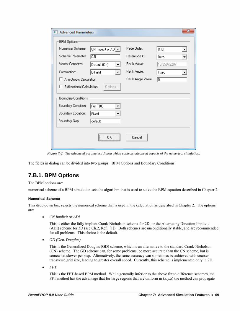
BeamPROP 8.0 User Guide Chapter 7: Advanced Simulation Features • 69
Figure 7-2. The advanced parameters dialog which controls advanced aspects of the numerical simulation.
The fields in dialog can be divided into two groups: BPM Options and Boundary Conditions:
7.B.1. BPM Options The BPM options are:
numerical scheme of a BPM simulation sets the algorithm that is used to solve the BPM equation described in Chapter 2.
Numerical Scheme
This drop down box selects the numerical scheme that is used in the calculation as described in Chapter 2. The options are:
• CN Implicit or ADI
This is either the fully implicit Crank-Nicholson scheme for 2D, or the Alternating Direction Implicit (ADI) scheme for 3D (see Ch.2, Ref. [1]). Both schemes are unconditionally stable, and are recommended for all problems. This choice is the default.
• GD (Gen. Douglas)
This is the Generalized Douglas (GD) scheme, which is an alternative to the standard Crank-Nicholson (CN) scheme. The GD scheme can, for some problems, be more accurate than the CN scheme, but is somewhat slower per step. Alternatively, the same accuracy can sometimes be achieved with coarser transverse grid size, leading to greater overall speed. Currently, this scheme is implemented only in 2D.
• FFT
This is the FFT-based BPM method. While generally inferior to the above finite-difference schemes, the FFT method has the advantage that for large regions that are uniform in (x,y,z) the method can propagate

70 • Chapter 7: Advanced Simulation Features BeamPROP 8.0 User Guide
the field in one step (provided also that the field does not significantly impinge on the boundary since transparent boundary conditions can not be employed). This method is most useful in conjunction with the simulation region feature discussed in Section 7.D and the tutorial example referenced there. Note that this method requires that the number of grid points in the transverse direction be a power of 2. This is automatically enforced by the program by padding the simulation domain. In addition, as noted above, this method does not employ transparent boundary conditions. This method is not recommended except for special circumstances as in the example referred to above.
Scheme Parameter
This sets the scheme parameter for the beam propagation calculation. In general it should be left at the default value of 0.5, except for 3D full-vector calculations where it may be necessary to choose a value between 0.5 and 1.0 to ensure stability. Refer to Section 7.A for further details on vector beam propagation. Refer to the guidelines in Section 2.C.2 for additional comments on use of the scheme parameter. Please contact RSoft if you have any questions about its use.
Vector Conserve
the basic vector BPM formulation described in Chapter 2 can have difficulty conserving power in some cases such as 2D TM or TE/TM for semi- or full-vector calculations. The software offers an improved vector BPM formulation that is enabled through the Vector Conserve option which can in many cases remedy the difficulties with power conservation, at a moderate cost in efficiency. This option is enabled by default, and can be also controlled by setting the variable vector_conserve to 0 or 1. This option is not currently enabled for full-vector or nonlinear calculations.
Formulation
This option sets whether the formulation is based on the electric field or magnetic field. While using the magnetic field formulation can sometimes offers better performance with respect to convergence and boundary conditions, not all capabilities of the program are enabled for this formulation. This option should be used by advanced users only.
Anisotropic Calculation
This option indicates that an anisotropic calculation should be performed. It requires that the Vector Mode be set to Full in the BeamPROP Simulation Parameters dialog. One or more refractive index tensors corresponding to the properties of the media can be defined as discussed in the CAD manual.
Bidirectional Calculation
This enables the use of the bidirectional feature in BeamPROP, and is discussed in Section 7.C.
Padé Order
The Padé Order drop down box selects the order of the Padé approximation that is used in the calculation. As described in Chapter 2, higher order approximations increase the accuracy of the results for large angles or large refractive index differences, but the computation time increases in proportion to the first number in the Padé order. The available choices are:
• (1,0)
This (1,0) approximation is equivalent to the standard paraxial or parabolic approximation, as described in Chapter 1.
• (1,1)
This (1,1) approximation generally produces better results than the (1,0) case, and takes no more computation time.
• (2,2)
• (3,3)
(4,4)
These approximations offer more accuracy at the expense of computation time as noted above.
BeamPROP 8.0 User Guide Chapter 7: Advanced Simulation Features • 71
In 3D, the wide-angle feature is generally not currently available. However for scalar 3D calculations an approximate version of the (1,1) option, valid for low-index contrast, has been implemented. In some test cases, this option has produced marked improvement over the (1,0) option, but should be used with caution since it can sometimes lead to less accurate results.
Only Padé (1,0) should be used when doing any form of mode calculation.
Reference k The reference k is the characteristic wavenumber used by the beam propagation method as described in Section 2.B.1.
Reference k
This field consists of a drop down box listing the available options, and a numeric input field labeled Reference k Value which contains the actual value to be used. The options are:
• k External
0 0k k n=
where 0k is the free space wavelength and 0n is the background index.
• k Average
0k k n=
where 0k is the free space wavelength and n represents an average index for the circuit.
• Beta
k β=
where β is an estimate of the propagation constant for the fundamental waveguide mode.
• Other
The value is specified by the user in the accompanying Reference k Value field.
Reference k Value
This field displays the value of the reference k to be used for the simulation. This value can only be changed if the Reference k is set to Other.
Reference k Angle
This field allows the characteristic wavenumber to be corrected for propagation at an angle. The characteristic wavenumber determined by the Reference k input field described above is multiplied by the cosine of the reference angle determined by this field, which must be a non-negative number measured in degrees from the Z axis. This field consists of a drop down box listing the available options, and a numeric input field labeled Reference k Angle Value which contains the specified reference angle. The options are:
• Fixed
The reference angle is fixed throughout the calculation and is determined by the value in the Reference k Angle Value field.
• Variable
The reference angle is allowed to vary throughout the calculation and is determined automatically by a weighted average of the local waveguide angles present in the circuit. Alternatively, the user can control

72 • Chapter 7: Advanced Simulation Features BeamPROP 8.0 User Guide
the local reference angle by defining an optical pathway and setting the kbar_path variable in the symbol table to be to desired pathway number.
Reference k Angle Value
This field sets the Reference k Angle Value to be used in conjunction with the Reference k Angle option. This default value for this field is 0.
7.B.2. Boundary Conditions There are several fields which set the type of boundary condition to be used during a simulation.
Boundary Condition
This drop down box selects the type of boundary condition employed in the calculation. The options are:
• Dirichlet
The field is required to be zero on the boundary. This effectively reflects radiation back into the computational domain.
• Simple TBC
This is the simple implementation of the transparent boundary condition as described in Ch. 2, Ref. [2]. It effectively lets radiation pass through the boundary and leave the computational domain. This choice is recommended for highly multimode problems.
• Full TBC This is the full implementation of the transparent boundary condition as described in Ch.2 Ref. [2]. It effectively lets radiation pass through the boundary and leave the computational domain. This choice is the default. However, in problems with a large amount of radiation this option can sometimes behave poorly, and the Simple TBC can perform better. For example, the Simple TBC is recommended for highly multimode problems.
Boundary Location
This drop down box is used in determining the boundary of the computational domain along the x axis. The options are:
• Fixed
The left and right boundary locations are fixed throughout the calculation, and are determined by the Domain Min and Domain Max fields described above. The default values for these fields are determined by the extent of the waveguide circuit and the Boundary Gap field described below.
• Variable
The left and right boundary locations are allowed to vary throughout the calculation, and are determined by the local extent of the waveguide circuit and the Boundary Gap field described below. Alternatively, the user can control the local left and right boundary locations by defining optical pathways and setting the boundary_path or boundary_path_left and boundary_path_right variables in the symbol table.
Please note this option is only implemented in 2D.
Boundary Gap
This numeric input field determines the gap between the extent of the waveguide circuit, and the recommended computational boundary. The default value is estimated by the program and is specified by the keyword default.
Other Boundary Types By default, the boundary condition selected by this option is applied to all boundaries. It can be useful, however, to apply different conditions at different boundaries. BeamPROP has this capability, and it is accessed through the symbol
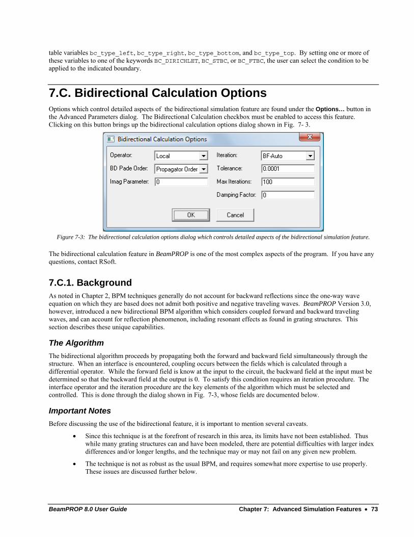
BeamPROP 8.0 User Guide Chapter 7: Advanced Simulation Features • 73
table variables bc_type_left, bc_type_right, bc_type_bottom, and bc_type_top. By setting one or more of these variables to one of the keywords BC_DIRICHLET, BC_STBC, or BC_FTBC, the user can select the condition to be applied to the indicated boundary.
7.C. Bidirectional Calculation Options Options which control detailed aspects of the bidirectional simulation feature are found under the Options… button in the Advanced Parameters dialog. The Bidirectional Calculation checkbox must be enabled to access this feature. Clicking on this button brings up the bidirectional calculation options dialog shown in Fig. 7- 3.
Figure 7-3: The bidirectional calculation options dialog which controls detailed aspects of the bidirectional simulation feature.
The bidirectional calculation feature in BeamPROP is one of the most complex aspects of the program. If you have any questions, contact RSoft.
7.C.1. Background As noted in Chapter 2, BPM techniques generally do not account for backward reflections since the one-way wave equation on which they are based does not admit both positive and negative traveling waves. BeamPROP Version 3.0, however, introduced a new bidirectional BPM algorithm which considers coupled forward and backward traveling waves, and can account for reflection phenomenon, including resonant effects as found in grating structures. This section describes these unique capabilities.
The Algorithm The bidirectional algorithm proceeds by propagating both the forward and backward field simultaneously through the structure. When an interface is encountered, coupling occurs between the fields which is calculated through a differential operator. While the forward field is know at the input to the circuit, the backward field at the input must be determined so that the backward field at the output is 0. To satisfy this condition requires an iteration procedure. The interface operator and the iteration procedure are the key elements of the algorithm which must be selected and controlled. This is done through the dialog shown in Fig. 7-3, whose fields are documented below.
Important Notes Before discussing the use of the bidirectional feature, it is important to mention several caveats.
• Since this technique is at the forefront of research in this area, its limits have not been established. Thus while many grating structures can and have been modeled, there are potential difficulties with larger index differences and/or longer lengths, and the technique may or may not fail on any given new problem.
• The technique is not as robust as the usual BPM, and requires somewhat more expertise to use properly. These issues are discussed further below.
74 • Chapter 7: Advanced Simulation Features BeamPROP 8.0 User Guide
• While this new feature does have its difficulties on some problems, we feel that its remarkable success on other problems which are of practical interest warrants its inclusion in BeamPROP, since it allows the user to accomplish calculations which would otherwise not be done.
• Normally all BeamPROP simulation results represent the electric field, E. However, in the case of bidirectional simulations with TM polarization, the software automatically switches to a calculation mode in which the field being simulated and displayed is the magnetic field, H.
• Currently, the bidirectional feature is only implemented for 2D geometries.
7.C.2. Enabling a Bidirectional BPM Simulation To use the bidirectional BPM feature, first create the desired circuit as usual. If you are creating a grating structure, note that periodic index or dimensional perturbations can be achieved in a single waveguide section by using a user-defined taper with the appropriate periodic functions (e.g. sin(x) or step(x) - see CAD manual appendices for more information on the built in functions available). Refer to the file grating.ind for an example.
Once the circuit has been created, it is recommended that before enabling the bidirectional feature, the circuit be simulated with the standard BPM in order to determine reasonable numerical parameters. One of the restrictions of the current bidirectional implementation is that transparent boundary conditions are not available, therefore it is important at this stage to set the domain large enough so that the amount of radiation hitting the boundary is small.
To perform a bidirectional simulation, first enable the bidirectional feature by selecting the Bidirectional Calculation check box in the Advanced Parameters dialog. Then initiate a simulation as usual by clicking on the green light icon, selecting numerical parameters in the simulation parameters dialog, and pressing OK.
For the simplest problems involving small index differences, the above is sufficient. More complex problems, however, require setting advanced options which is done through the Options… button in the Advanced Parameters dialog. This is discussed further below, but first we consider some more general issues connected with the bidirectional feature.
An Example It would be instructive at this point to open the grating.ind example file, and run the simulation as described above. There are several points to note.
• The display mode is set to Slices, which is the only display currently available with the bidirectional feature.
• The display is the usual one, except that in addition to displaying the forward field in blue, the backward field is displayed in green.
• The calculation proceeds forward and backward one or more times, reflecting the iterative nature of the technique. Note that under some conditions, the display may pause for long periods during internal iterations.
• The monitor has been set to display the power in the reflected field. This is done by setting the Monitor Component field in the monitors dialog to be Major - Backward. See Chapter 5 for a discussion of this option, as well as monitors in general.
7.C.3. Bidirectional Parameters This section documents the fields shown in Fig. 7-3.
Operator
This field selects the operator which is used at longitudinal interfaces to couple the forward and backward fields. The default choice is Local, which is corresponds to an approximation valid for low index contrast structures. The second choice is Padé, which uses that technique to achieve a better approximation appropriate to higher index contrast cases. In this case, it is important to carefully set the BD Padé Order and Imag Parameter fields described below, as well as

BeamPROP 8.0 User Guide Chapter 7: Advanced Simulation Features • 75
the Padé Order field in the advanced numerical parameters dialog which is important for the propagation part of the calculation.
BD Padé Order
This field defines the order of the Padé-based interface operator, and is analogous to the Padé Order field in the Advanced Numerical Parameters dialog. The default choice is Propagator Order, which means that the order used in the interface operator is equal to the order used in propagation set via the Advanced…dialog discussed in Section 7.B.
The other choices are the same as those described in Section 7.B.1 for wide-angle propagation. In general, for high contrast cases the Padé technique must be used for both the interface and the propagation, but the orders need not be the same. The order required for the propagation is that necessary to accurately propagate the phase of the wave between interfaces in order to accurately model resonant reflection effects in a grating for example. The order required for the interface operator is primarily determined by the need to deal with a wide range of k-vectors in the complex plane associated with the Imag Parameter field described below.
Imag Parameter
This field defines a parameter associated with controlling the stability of the Padé-based interface operator. When using this operator, artificial evanescent waves are generated during the calculation which lead to instability. True evanescent waves, however, are also generated which are not a problem.
To circumvent this, an imaginary component is added to the reference wavenumber which effectively damps the artificial evanescent waves. This field controls the stabilization parameter, which must be between 0 and 1. It is best to choose as small a stabilization parameter as possible, since a large value of the parameter affects the true solution in addition to damping the artificial solution. The latter difficulty is circumvented by employing a higher Padé order for the interface operator, which allows accurate computations with a large stabilization parameter. For a high index contrast problem, a typical imaginary parameter is 0.6-0.8, and an appropriate Padé order is (2,2) or (3,3).
Iteration
This field selects the iteration procedure used in the bidirectional calculations. The options are as follows:
• BF-Fixed
BF-Auto
These options refer to a proprietary iteration technique. Each option is controlled by a stabilization parameter (see the Damping Factor field below), which is help fixed in the BF-Fixed option, and is dynamically adjusted in the BF-Auto option. This option generally works best for the simplest problems, and is currently the default. For high index problems the Matrix option described below is recommended.
• Matrix
Matrix-2
Matrix-3
These options uses standard iteration techniques for solving linear systems, the details of which are proprietary. These options are generally more robust than the BF options above, but can be slower on many problems. For high index problems, use of these options is highly recommended. Matrix or Matrix-3 are generally best. Matrix-3 is the most robust, but is sometimes slower than Matrix. Matrix-2 is generally not recommended.
The default is currently BF-Auto, although this may be changed in subsequent releases.
Tolerance
This field defines the convergence criterion for the iteration. The iteration stops when the normalized power in the backward field at the output of the circuit is less than the tolerance value set in this field (the backward power is normalized to the forward input power). The default value is 10e-4. The iteration also terminates after a specified maximum number of iterations, defined in the Max Iterations field described below.
76 • Chapter 7: Advanced Simulation Features BeamPROP 8.0 User Guide
Max Iterations
This field limits the number of iterations to the specified value. The default limit is 100 iterations.
Damping Factor
This field defines a stabilization parameter related to the BF-Fixed and BF-Auto iteration options. The value should be between 0 and 1, and the default of 0 indicates no damping. In the case of the BF-Fixed iteration option, this value defines the damping factor throughout the iteration. For the BF-Auto iteration option, this value defines the initial damping factor, and the damping factor is adjusted dynamically during the simulation as required. If the default of 0 yields difficulties, a good alternative starting value is 0.5.
7.D. Defining Simulation Regions The BPM technique gains much of its speed by leveraging the fact that for many photonic device simulations the variation of the structure along the propagation direction is small to moderate. By choosing an appropriate step size, reference wavenumber, Pade order, etc. one can get accurate results in a reasonable length of time in such structures. Guidelines for the choice of these parameters can be found in Chapter 2.
7.D.1. Why Use a Simulation Region? Some structures can have large variations along the propagation direction. An example would be propagation from a waveguide into free space, through a lens, and back into another waveguide. This type of problem has two difficulties.
• The first problem is that there will be reflections at the interfaces that must be taken into account. This might be amenable to bidirectional BPM; alternatively in many cases it can be accounted for approximately by a simple Fresnel correction.
• The second problem is that the large change in index means that each region along z has a different set of optimum simulation parameters.
To solve the problem, one can find a compromise for the best reference wavenumber, choose a higher Pade order to make the problem less dependent on the index variation, and choose a step size small enough to accommodate all regions. While this generally works, the simulation time suffers.
Fortunately, BeamPROP has a feature called “Simulation Regions” which allows the user to define multiple regions along the propagation direction and within each region provide local control of step size and other simulation parameters. This enables the user to optimize the calculation for a wide variety of structures.
7.D.2. Defining a Simulation Region The procedure for defining a simulation region is similar to that for drawing a waveguide segment. From the left toolbar, select the simulation region icon, or SimRegion Mode. Then use the mouse as if you were drawing a waveguide segment from the starting Z location to the ending Z location over which you want to define the region (the X position does not matter as the simulation region effectively has infinite extent in X).
Features such as logical attachment, referencing, etc. that are available for positioning waveguide segments are also available for simulation regions. Alternatively, a simulation region can be defined by choosing Options/Insert/Simulation-Region. In this dialog, you must define the starting and ending Z position of the region as in the segment properties dialog. After pressing OK, the region is entered. After creating the simulation region via either method, you may want to choose Edit/Change-Order/To-Back if the region obscures any waveguides that were previously drawn.
Creating Local Simulation Parameters Once the region has been created, to define the local simulation properties of the region, right click on the region and select Local Symbols… to open up the familiar symbol table editor. This is just like the normal, global symbol table, which is also accessible in the simulation region properties; however variables defined in the local symbol table override

BeamPROP 8.0 User Guide Chapter 7: Advanced Simulation Features • 77
those in the global table. The local symbol table will initially be empty. To locally set a parameter, such as the Z Compute Step, add the appropriate symbol as a new variable and give it the desired value. Currently, the overrides that are possible are as follows: Variable Definition
step_size Z Compute Step size kbar Reference k kbar_angle Reference k Angle pade_order Padé Order (0-4) simulated_bend Enable/disable Simulated bend (0/1) simulated_bend_radius Set Simulated Bend Radius(can be +/-) scheme Simulation Method (SCHEME_CN,...)
The variables have their usual meaning, as indicated above.
In addition to typical simulation parameters such as step size, control over other simulation aspects, such as the simulation method, is possible. For example, propagation through a long free space region can be done via the FFT-based BPM method by setting scheme = SCHEME_FT in the symbol table.
A tutorial example describing the use of the simulation region feature is given in Tutorial 11.
7.E. Anisotropy, Non-Linearity, and Dispersion BeamPROP supports the following material properties:
A detailed description of how these properties are defined in the CAD can be found in Chapter 8 of the CAD manual.
• Anisotropy
BeamPROP can incorporate anisotropic materials in order to simulation birefringent effects. Note that the Vector Mode must be set to Full as discussed in Section 7.A in order to perform an anisotropic simulation.
• Non-Linearity
BeamPROP can incorporate 3χ or n2 nonlinearity on a single, monochromatic wave in order to address certain types of guided-wave nonlinear optics problems. Thus, devices such as nonlinear directional couplers and spatial solitons, or temporal solitons via a change of variables, can be modeled. The CAD manual describes several methods of defining the non-linear parameters.
• Dispersion
BeamPROP performs monochromatic simulations at single wavelengths. Thus, it cannot include dispersive effects within a single simulation. However, by defining the refractive index as a function of wavelength, a parameter scan over wavelength can be used to analyze dispersive materials. The CAD manual describes several methods to accomplish this.
7.F. Calculation Electrodes/Heater Effects BeamPROP includes a capability for incorporating the effects of electrodes or heaters With this feature, Poisson's equation is solved to determine the potential or temperature profile. The electro-optic or thermo-optic effects are then used to determine the perturbation to the refractive index profile. Finally, this perturbation is incorporated directly into the beam propagation calculations. The example file electrode.ind demonstrates this capability via a Mach-Zehnder
78 • Chapter 7: Advanced Simulation Features BeamPROP 8.0 User Guide
modulator composed of channel waveguides and three electrodes in a push-pull geometry. This section describes the use of this feature.
There are essentially two required parts to defining an electrode/heater problem:
• Define the electro/thermo-optic materials in which the electrodes/heaters are embedded.
• Define the electrodes/heaters themselves.
For simplification, the remainder of the discussion will focus on electrodes, except as noted.
7.F.1. Defining Electro-Optic Material The first step is accomplished via the Electrode Header Layer Table shown in Fig. 7-3. This table can be accessed via the menu option Edit/Tables/Edit-Electrode/Heater-Layers. The model is currently restricted to simple multilayer geometries, so that lateral variations in the dielectric constant are not included in the electrode modeling, although they are included in the optical modeling, and any 3D Structure Type for optical modeling can be used with the electrode feature.
Figure 7-3: The electrode/heater layer table editor dialog, which defines the electro/thermo-optic materials in which the
electrodes/heaters are embedded.
This dialog allows construction of a layer table in which each layer contains the following information: Field Description Height thickness of the layer Eps X relative dielectric constant in X Eps Y relative dielectric constant in Y Rx electro-optic coefficient multiplying Ex Ry electro-optic coefficient multiplying Ey N0 optical index of the layer
Layer 0 corresponds to the substrate, and the last layer defined corresponds to the cover. The thickness of all the layers together determines the computational domain in the vertical direction.

BeamPROP 8.0 User Guide Chapter 7: Advanced Simulation Features • 79
Computing the Index Perturbation The index perturbation is computed from
( )( )( ) ( )( )( )
⎟⎟⎠
⎞⎜⎜⎝
⎛+−=Δ
20
20 33
yx ERYNERXNn
where xE and xE are the horizontal and vertical fields from the electrodes. The fields are calculated in V/μm, so the R coefficients must be given in μm/V.
Heater Definition For the thermal case, Eps is replaced by Kappa, the thermal conductivity. The required units are W/(μm*K). The RX field in the dialog should contain the temperature coefficient for index change, i.e. dn/dT. The remaining fields RY and N0 are not used in the thermal case. The index perturbation is computed from
Tdtdnn Δ=Δ
where TΔ is the computed temperature rise relative to the bottom of the substrate layer, which is held at T=0. The units of RX (dn/dT) are 1/K.
7.F.2. Creating Electrodes/Heaters in the CAD The creation of the electrodes is accomplished via the CAD layout by drawing a straight waveguide segment at the desired position of the electrode and with the desired length.
After drawing the waveguide, it is turned into an electrode by right clicking on it to edit its properties, and performing the following steps:
1. Set the Profile Type to Inactive.
2. Set the Component Width and Component Height of the electrode as desired. The electrode is always rectangular, and the height can be 0. Set the desired vertical position of the electrode via the Y Position field.
3. Click on the More… button to access the Additional Component Properties dialog, and select the desired Electrode/Heater Type and the E/H Control Parameter. These parameters are defined below.
Electrode/Heater Types There are three types of Electrode/Heaters, each with an E/H Control Parameter:
• Electrode – This choice corresponds to an electrode or voltage source. Its E/H Control Parameter is an applied voltage V given in units of Volts.
• Temperature - This choice corresponds to a thermal heater, or temperature source. Its E/H Control Parameter is a temperature rise in degrees Kelvin.
• Heat – This choice corresponds to a thermal heater, or heat source. Its E/H Control Parameter is the following heat parameter:
The heat parameter is given by ρ*I2, where ρ is the resistivity in Ω-μm, and I is the current in A (Amperes). For a surface source (height=0 and located at the top of the cover layer), the heat parameter should be ρ*I2/h, where h is the actual small but finite height of the heater.
The control parameter field can contain an expression using variables, as in all BeamPROP parameter fields. Also, any number of electrodes/heaters may be defined, and that, for calculation efficiency, groups of electrodes may be defined using Pathways.
80 • Chapter 7: Advanced Simulation Features BeamPROP 8.0 User Guide
7.F.3. Using the Electrode/Heater Utility The above steps describe how to set up an electrode problem. By running a normal BeamPROP calculation, the electric field or temperature profile will be computed automatically by the Electrode/Heather utility, and used to add an index perturbation to the rest of the index profile.
You can also run the Electrode/Heater utility separately, as well as set some of the numerical parameters to be used in the simulation, via the Utility/Electrode/Heater option in the CAD menu. This opens the dialog displayed in Fig. 7-4
Figure 7-4: The electrode/heater utility dialog.
After running this utility, the potential or temperature profile will be displayed, and other data will be available from the WinPLOT icon. The available graph files are, where <prefix> is the specified Output File Prefix: File Description
<prefix>.pt Temperature
<prefix>.pv Potential
<prefix>.pex Ex field
<prefix>.pey Ey field
<prefix>.ppf Index Perturbation
The dialog contains several settings for controlling the electrode simulation, which are also used when a normal BeamPROP calculation is performed. These include the tolerance for the iteration and the x and y grid sizes. In addition there is an acceleration parameter that can be controlled by setting the variable electrode_a. If you have difficulty converging, try setting this parameter to a value between 1 and 3 (the default is 1).
7.F.4. Additional Notes There are several additional items to note regarding the electrode feature.
• When the index profile is displayed, the effect of the electrodes is normally not included to avoid the delay due to the electrode calculation. However, by setting the variable electrode_enable to 1, the effect of the electrodes will be included in the display of the index profile. Similarly, setting electrode_enable to 0 will disable the electrode calculation in a normal simulation. The default setting of electrode_enable is 1 when performing a simulation, and 0 when displaying the index.
• The electrode feature can be used in conjunction with mode calculations. The effect of the index perturbation will automatically be included in the effective index of the mode, which is useful for designing the proper voltage/temperature or electrode position to achieve a certain change in effective index.
BeamPROP 8.0 User Guide Chapter 7: Advanced Simulation Features • 81
• Electrodes or heaters may be tilted or curved. This is done internally by automatically translating the center of the potential/temperature profile (which is calculated at the beginning of the electrode/heater group). This is only accurate for shallow angles, and the electrode/heater structure is still required to have constant width and/or spacing. There are also grouping restrictions as noted below.
• The electrodes/heaters may be placed in separate groups which can optimize the calculation by isolating different collections of electrodes which should not interact. Grouping is done by selecting the desired electrodes/heaters into one or more pathways, as described in the CAD manual. All electrodes/heaters not selected into a pathways are placed in the default group. The first pathway containing electrodes/heaters would be group 1, the second would be group 2, etc. The default group would be the number following the last defined group, or 1 if no groups are explicitly defined.
Currently, all electrodes in a group are required to start and end at the same Z position. Thus an electrode consisting of a straight waveguide followed by a tilted waveguide should have each electrode in a separate group. The feature that allows tilted or curved waveguides currently requires this.
7.G. Radial BPM BeamPROP includes an option for Radial BPM, which allows certain 3D problems with aximuthal symmetry to be simulated as 2D problems. This creates a simulation with an efficiency close to a 2D problem since the azimuthal dependence is treated analytically and only the radial (R) and axial (Z) coordinates are treated numerically. To enable the Radial BPM feature, either check Radial Calculation in the Global Settings dialog, or define the variable radial and set it to 1 in the symbol table.
Older versions of BeamPROP selected a Radial BPM simulation via the Numerical Scheme field in the Advanced Simulation Parameters dialog. This is no longer the case, and old files which used the option will automatically be converted as appropriate to use the new method of selection. The method itself has not changed.
Selecting Radial Calculation in the Global Settings dialog enables a radial version of the Crank-Nicholson scheme for 2D, meaning that the propagation is done in cylindrical (r,z) coordinates. For problems with circular symmetry in both the structure and the launch field, this Radial BPM option is equivalent to a full scalar 3D BPM, but significantly faster (usually by several orders of magnitude).
7.G.1 Using Radial BPM To use this option, choose a 2D waveguide model and consider X=0 as the center of symmetry when defining the structure. When this scheme is selected, the transverse coordinate X is then interpreted as the radial coordinate R. Note that while the structure can be defined for X<0 and X >0, and this is in general the optimal things to do , the problem will only be solved in the half space X>0. The user need not select this – the program will automatically enforce it.
While it is implied that the structure is azimuthally symmetric, the field can have other implied azimuthal behavior. The variable azimuthal_mode controls the azimuthal dependence which is assumed to be φime , where m is the value of azimuthal_mode and φ is the polar angle. The azimuthal_mode variable effects the radial propagation, mode shape, and propagation constants appropriately, so that, for example, antisymmetric modes with m=1 can be calculated by setting azimuthal_mode=1.
Note that when using a Launch Type of Fiber Mode for a radial calculation indicates that a LP mode should be used. It is not currently possible to launch a genuine TE or TM mode.
7.G.2. Displaying 3D Results The azimuthal pattern is normally not displayed unless a result from a Radial calculation is launched into a 3D calculation. However, there is a feature which allows modes and output fields calculated using Radial BPM to be

82 • Chapter 7: Advanced Simulation Features BeamPROP 8.0 User Guide
automatically output as 3D data files and graphs. By setting Output Radial Data in XY Format option in the Output Options dialog, in addition to any 2D radial files that are generated, corresponding 3D results will be generated whose file prefix will be the original file prefix with “_3d” appended. Note that it is not necessary to use this option to generate results for input to a 3D calculation, as the 3D BPM will automatically read the 2D radial files and generate the 3D field internally. The main purpose of this option is to allow visualization of the radial fields as contour plots. Note also that any azimuthal behavior that was implicit in the radial calculation is reflected in the 3D data file and graph.
7.H. Effective Index Calculations Both the startup dialog and the global settings dialog contain a check box labeled Effective Index Calculation. When this option is selected, before performing a simulation BeamPROP automatically converts the 3D waveguide circuit that has been defined into an approximately equivalent 2D circuit using the well-known effective index method (EIM).
The EIM technique greatly reduces the computation time and memory requirements of the simulation, however the results will be less accurate than for a full 3D simulation. Note that this feature is currently only supported for the Diffused and Rib/Ridge 3D structures. Finally, note that the 3D to 2D conversion that occurs when selecting this option only affects the simulation; the definition of the original 3D circuit is unaltered. Thus the user can safely switch this feature on and off without changing the circuit that has been defined.
BeamPROP 8.0 User Guide Chapter 8: Basic Tutorials • 83
Chapter 8: Basic Tutorials
This chapter contains several basic tutorial examples which illustrate the basic use of the BeamPROP simulation engine. These tutorials are increasingly complex and many of them build on concepts established in earlier tutorials. It is important that you perform them in order, even if a particular topic is of most interest to you. It is also recommended that users work through the basic tutorials in this chapter before moving to the advanced tutorials in Chapter 9.
These tutorials do not have associated .ind files.
Basic Tutorial 1: Basic 2D Simulation This tutorial illustrates basic CAD layout features by creating a new circuit and demonstrates a sample workflow to perform a simulation and obtain simulation results. Our goal will be to layout and simulate the propagation of a mode at 1.55 µm along a single 2D slab waveguide with a cladding index of 1, a core index of 1.1, and a width of 7 µm. We will calculate the transmitted power along 1000 µm of this waveguide.
This tutorial will introduce basic concepts about the RSoft CAD interface and the BeamPROP simulation engine that are critical for every user to understand; it is recommended that every new user work through this tutorial. For additional information about the RSoft CAD, please consult the CAD manual.
CAD Window Basics We begin by opening up the RSoft CAD window. Windows users can do this via the Start menu and Linux users can issue the command xbcad at a command prompt.
The CAD window, shown in Fig. 1, contains the following elements:
• A menubar near the top of the window
The menubar allows access to various standard file and editing operations such as opening and saving index files and cutting and pasting waveguide components in a circuit.
• Two toolbars with icons just below the menubar
The top toolbars contain icons for standard file, editing, and viewing operations.
•
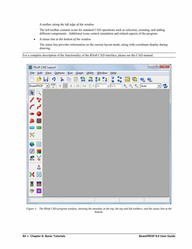
84 • Chapter 8: Basic Tutorials BeamPROP 8.0 User Guide
A toolbar along the left edge of the window
The left toolbar contains icons for standard CAD operations such as selection, zooming, and adding different components. Additional icons control simulation and related aspects of the program.
• A status line at the bottom of the window
The status line provides information on the current layout mode, along with coordinate display during drawing.
For a complete description of the functionality of the RSoft CAD interface, please see the CAD manual.
Figure 1: The RSoft CAD program window, showing the menubar at the top, the top and left toolbars, and the status line at the bottom.
BeamPROP 8.0 User Guide Chapter 8: Basic Tutorials • 85
Creating a New Circuit To create a new circuit, click on the New Circuit icon in the top toolbar (the leftmost icon on the top toolbar). Alternatively, choose File/New from the menu. The startup dialog appears, as shown in Fig. 2. This dialog requests basic information about the circuit to be modeled, including the wavelength of the light, the background refractive index, the default index change between the background material and the structure, and the approximate overall dimensions of the device.
Choosing Initial Settings: For this simulation, we will use the following settings: Parameter Value Description
Simulation Tool BeamPROP Indicates that the BeamPROP simulation engine should be used for this simulation.
Model Dimension 2D Indicates that a 2D simulation should be performed.
Free Space Wavelength 1.55 This is the global wavelength (in µm) to be used for the simulation.
Background Index 1.0 This represents the real refractive index of the background material where no structure has been defined.
Index Difference 0.1 This represents the default difference between a component and the background material. In this case this means that the structure will have an index of 1.1. This is simply the default value to be used for a component; each component can have a unique value if desired.
Component Width 7.0 This represents the default width of a component in µm. This is simply the default value to be used for a component; each component can have a unique value if desired.
Once these settings are made, click OK to continue. Note that changes can be made to these settings via the Global Settings dialog box which can be opened by clicking the ‘Globe’ icon in the left toolbar.
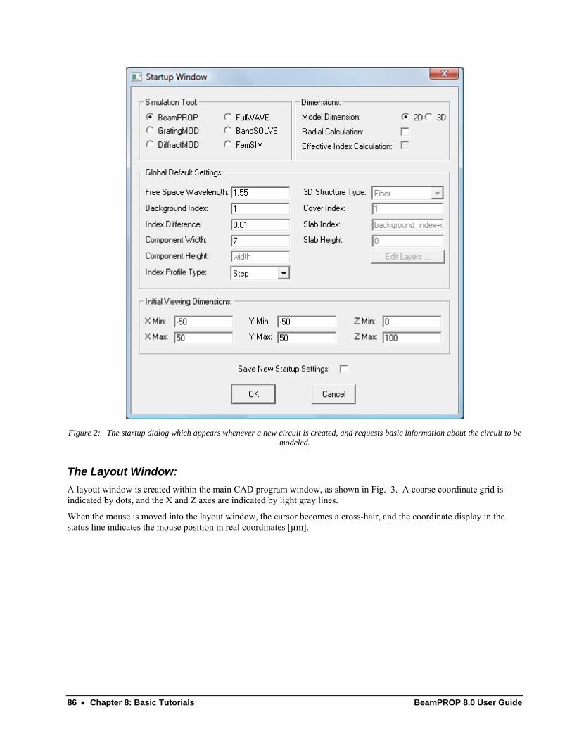
86 • Chapter 8: Basic Tutorials BeamPROP 8.0 User Guide
Figure 2: The startup dialog which appears whenever a new circuit is created, and requests basic information about the circuit to be modeled.
The Layout Window: A layout window is created within the main CAD program window, as shown in Fig. 3. A coarse coordinate grid is indicated by dots, and the X and Z axes are indicated by light gray lines.
When the mouse is moved into the layout window, the cursor becomes a cross-hair, and the coordinate display in the status line indicates the mouse position in real coordinates [µm].
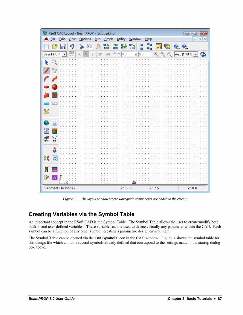
BeamPROP 8.0 User Guide Chapter 8: Basic Tutorials • 87
Figure 3: The layout window where waveguide components are added to the circuit.
Creating Variables via the Symbol Table An important concept in the RSoft CAD is the Symbol Table. The Symbol Table allows the user to create/modify both built-in and user-defined variables. These variables can be used to define virtually any parameter within the CAD. Each symbol can be a function of any other symbol, creating a parametric design environment.
The Symbol Table can be opened via the Edit Symbols icon in the CAD window. Figure 4 shows the symbol table for this design file which contains several symbols already defined that correspond to the settings made in the startup dialog box above.
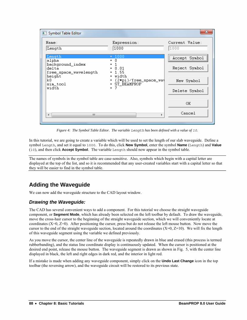
88 • Chapter 8: Basic Tutorials BeamPROP 8.0 User Guide
Figure 4: The Symbol Table Editor. The variable Length has been defined with a value of 10.
In this tutorial, we are going to create a variable which will be used to set the length of our slab waveguide. Define a symbol Length, and set it equal to 1000. To do this, click New Symbol, enter the symbol Name (Length) and Value (10), and then click Accept Symbol. The variable Length should now appear in the symbol table.
The names of symbols in the symbol table are case-sensitive. Also, symbols which begin with a capital letter are displayed at the top of the list, and so it is recommended that any user-created variables start with a capital letter so that they will be easier to find in the symbol table.
Adding the Waveguide We can now add the waveguide structure to the CAD layout window.
Drawing the Waveguide: The CAD has several convenient ways to add a component. For this tutorial we choose the straight waveguide component, or Segment Mode, which has already been selected on the left toolbar by default. To draw the waveguide, move the cross-hair cursor to the beginning of the straight waveguide section, which we will conveniently locate at coordinates (X=0, Z=0). After positioning the cursor, press but do not release the left mouse button. Now move the cursor to the end of the straight waveguide section, located around the coordinates (X=0, Z=10). We will fix the length of this waveguide segment using the variable we defined previously.
As you move the cursor, the center line of the waveguide is repeatedly drawn in blue and erased (this process is termed rubberbanding), and the status line coordinate display is continuously updated. When the cursor is positioned at the desired end point, release the mouse button. The waveguide segment is drawn as shown in Fig. 5, with the center line displayed in black, the left and right edges in dark red, and the interior in light red.
If a mistake is made when adding any waveguide component, simply click on the Undo Last Change icon in the top toolbar (the reversing arrow), and the waveguide circuit will be restored to its previous state.
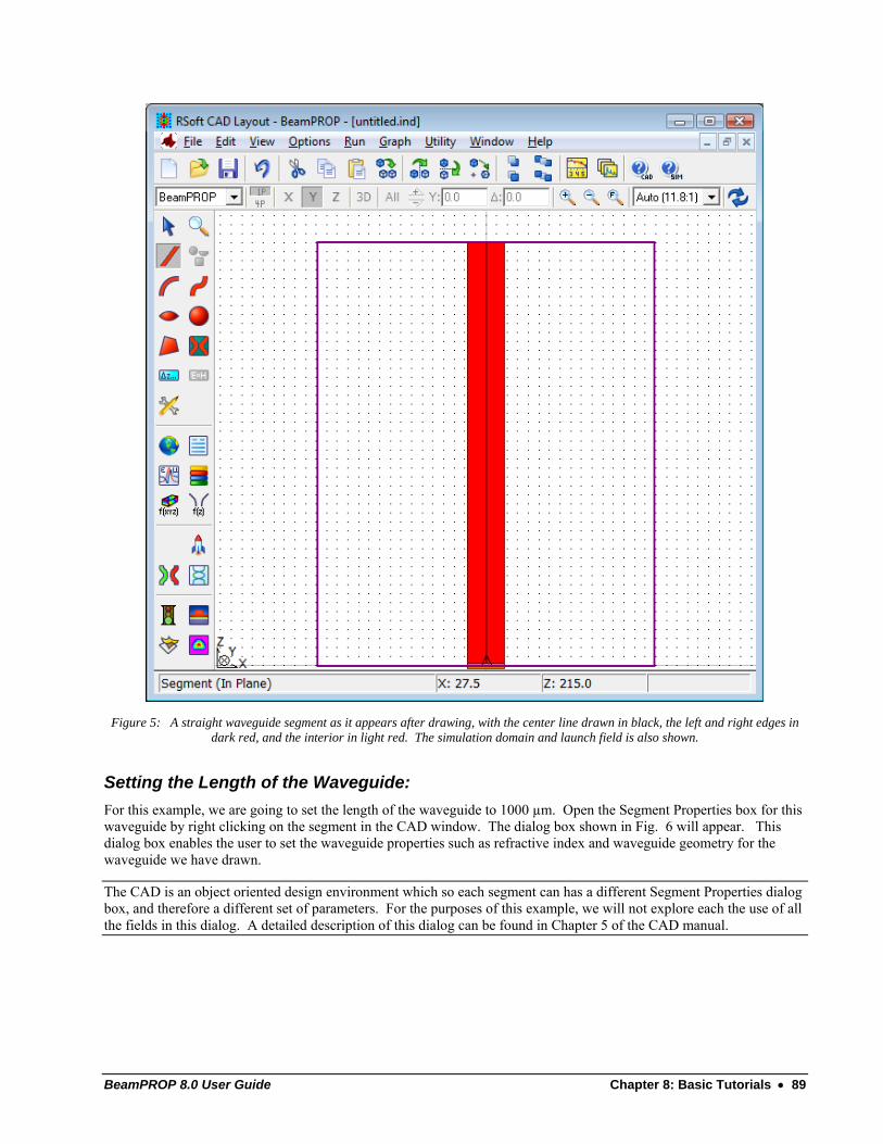
BeamPROP 8.0 User Guide Chapter 8: Basic Tutorials • 89
Figure 5: A straight waveguide segment as it appears after drawing, with the center line drawn in black, the left and right edges in dark red, and the interior in light red. The simulation domain and launch field is also shown.
Setting the Length of the Waveguide: For this example, we are going to set the length of the waveguide to 1000 µm. Open the Segment Properties box for this waveguide by right clicking on the segment in the CAD window. The dialog box shown in Fig. 6 will appear. This dialog box enables the user to set the waveguide properties such as refractive index and waveguide geometry for the waveguide we have drawn.
The CAD is an object oriented design environment which so each segment can has a different Segment Properties dialog box, and therefore a different set of parameters. For the purposes of this example, we will not explore each the use of all the fields in this dialog. A detailed description of this dialog can be found in Chapter 5 of the CAD manual.
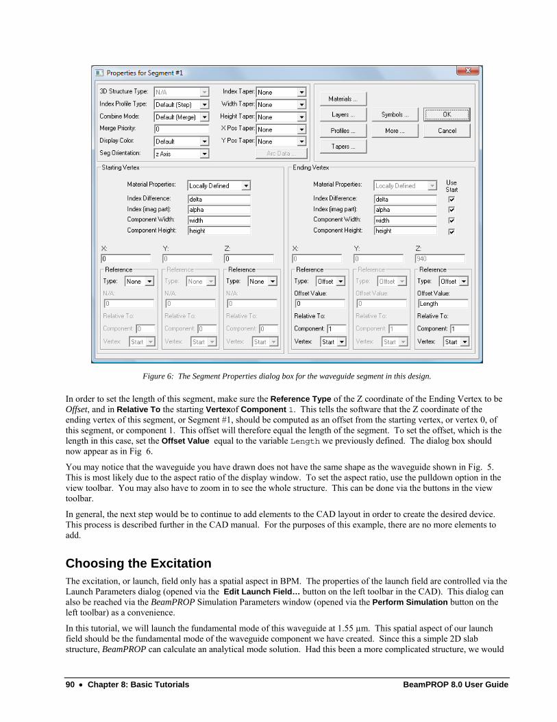
90 • Chapter 8: Basic Tutorials BeamPROP 8.0 User Guide
Figure 6: The Segment Properties dialog box for the waveguide segment in this design.
In order to set the length of this segment, make sure the Reference Type of the Z coordinate of the Ending Vertex to be Offset, and in Relative To the starting Vertexof Component 1. This tells the software that the Z coordinate of the ending vertex of this segment, or Segment #1, should be computed as an offset from the starting vertex, or vertex 0, of this segment, or component 1. This offset will therefore equal the length of the segment. To set the offset, which is the length in this case, set the Offset Value equal to the variable Length we previously defined. The dialog box should now appear as in Fig 6.
You may notice that the waveguide you have drawn does not have the same shape as the waveguide shown in Fig. 5. This is most likely due to the aspect ratio of the display window. To set the aspect ratio, use the pulldown option in the view toolbar. You may also have to zoom in to see the whole structure. This can be done via the buttons in the view toolbar.
In general, the next step would be to continue to add elements to the CAD layout in order to create the desired device. This process is described further in the CAD manual. For the purposes of this example, there are no more elements to add.
Choosing the Excitation The excitation, or launch, field only has a spatial aspect in BPM. The properties of the launch field are controlled via the Launch Parameters dialog (opened via the Edit Launch Field… button on the left toolbar in the CAD). This dialog can also be reached via the BeamPROP Simulation Parameters window (opened via the Perform Simulation button on the left toolbar) as a convenience.
In this tutorial, we will launch the fundamental mode of this waveguide at 1.55 µm. This spatial aspect of our launch field should be the fundamental mode of the waveguide component we have created. Since this a simple 2D slab structure, BeamPROP can calculate an analytical mode solution. Had this been a more complicated structure, we would
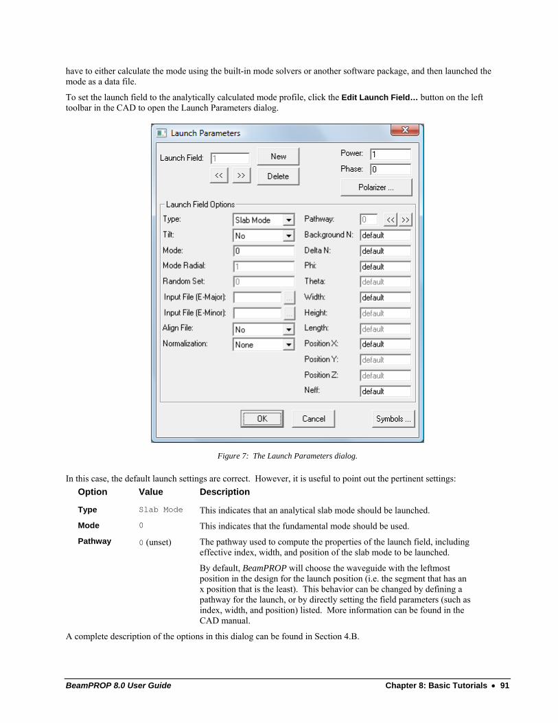
BeamPROP 8.0 User Guide Chapter 8: Basic Tutorials • 91
have to either calculate the mode using the built-in mode solvers or another software package, and then launched the mode as a data file.
To set the launch field to the analytically calculated mode profile, click the Edit Launch Field… button on the left toolbar in the CAD to open the Launch Parameters dialog.
Figure 7: The Launch Parameters dialog.
In this case, the default launch settings are correct. However, it is useful to point out the pertinent settings: Option Value Description
Type Slab Mode This indicates that an analytical slab mode should be launched.
Mode 0 This indicates that the fundamental mode should be used.
Pathway 0 (unset) The pathway used to compute the properties of the launch field, including effective index, width, and position of the slab mode to be launched.
By default, BeamPROP will choose the waveguide with the leftmost position in the design for the launch position (i.e. the segment that has an x position that is the least). This behavior can be changed by defining a pathway for the launch, or by directly setting the field parameters (such as index, width, and position) listed. More information can be found in the CAD manual.
A complete description of the options in this dialog can be found in Section 4.B.
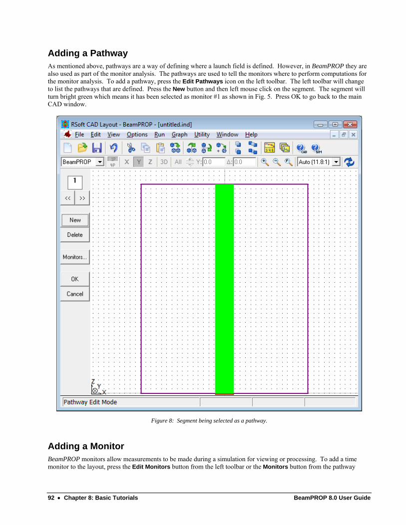
92 • Chapter 8: Basic Tutorials BeamPROP 8.0 User Guide
Adding a Pathway As mentioned above, pathways are a way of defining where a launch field is defined. However, in BeamPROP they are also used as part of the monitor analysis. The pathways are used to tell the monitors where to perform computations for the monitor analysis. To add a pathway, press the Edit Pathways icon on the left toolbar. The left toolbar will change to list the pathways that are defined. Press the New button and then left mouse click on the segment. The segment will turn bright green which means it has been selected as monitor #1 as shown in Fig. 5. Press OK to go back to the main CAD window.
Figure 8: Segment being selected as a pathway.
Adding a Monitor BeamPROP monitors allow measurements to be made during a simulation for viewing or processing. To add a time monitor to the layout, press the Edit Monitors button from the left toolbar or the Monitors button from the pathway
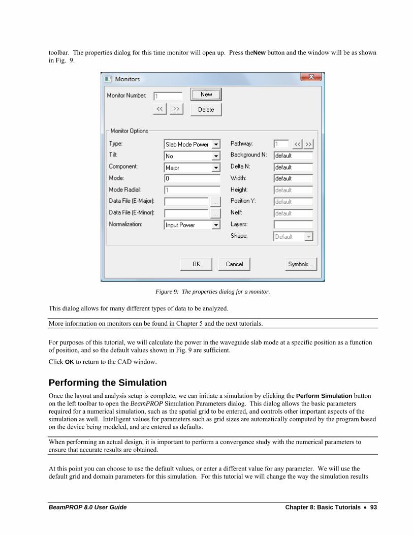
BeamPROP 8.0 User Guide Chapter 8: Basic Tutorials • 93
toolbar. The properties dialog for this time monitor will open up. Press theNew button and the window will be as shown in Fig. 9.
Figure 9: The properties dialog for a monitor.
This dialog allows for many different types of data to be analyzed.
More information on monitors can be found in Chapter 5 and the next tutorials.
For purposes of this tutorial, we will calculate the power in the waveguide slab mode at a specific position as a function of position, and so the default values shown in Fig. 9 are sufficient.
Click OK to return to the CAD window.
Performing the Simulation Once the layout and analysis setup is complete, we can initiate a simulation by clicking the Perform Simulation button on the left toolbar to open the BeamPROP Simulation Parameters dialog. This dialog allows the basic parameters required for a numerical simulation, such as the spatial grid to be entered, and controls other important aspects of the simulation as well. Intelligent values for parameters such as grid sizes are automatically computed by the program based on the device being modeled, and are entered as defaults.
When performing an actual design, it is important to perform a convergence study with the numerical parameters to ensure that accurate results are obtained.
At this point you can choose to use the default values, or enter a different value for any parameter. We will use the default grid and domain parameters for this simulation. For this tutorial we will change the way the simulation results
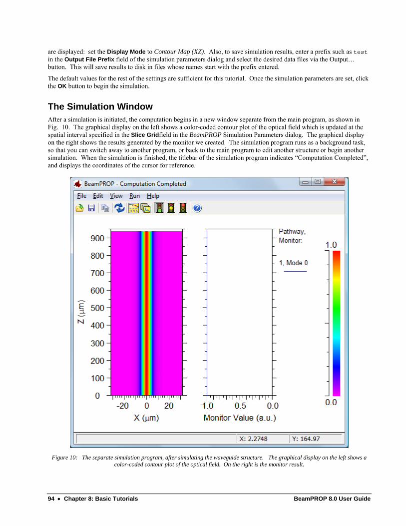
94 • Chapter 8: Basic Tutorials BeamPROP 8.0 User Guide
are displayed: set the Display Mode to Contour Map (XZ). Also, to save simulation results, enter a prefix such as test in the Output File Prefix field of the simulation parameters dialog and select the desired data files via the Output… button. This will save results to disk in files whose names start with the prefix entered.
The default values for the rest of the settings are sufficient for this tutorial. Once the simulation parameters are set, click the OK button to begin the simulation.
The Simulation Window After a simulation is initiated, the computation begins in a new window separate from the main program, as shown in Fig. 10. The graphical display on the left shows a color-coded contour plot of the optical field which is updated at the spatial interval specified in the Slice Gridfield in the BeamPROP Simulation Parameters dialog. The graphical display on the right shows the results generated by the monitor we created. The simulation program runs as a background task, so that you can switch away to another program, or back to the main program to edit another structure or begin another simulation. When the simulation is finished, the titlebar of the simulation program indicates “Computation Completed”, and displays the coordinates of the cursor for reference.
Figure 10: The separate simulation program, after simulating the waveguide structure. The graphical display on the left shows a color-coded contour plot of the optical field. On the right is the monitor result.
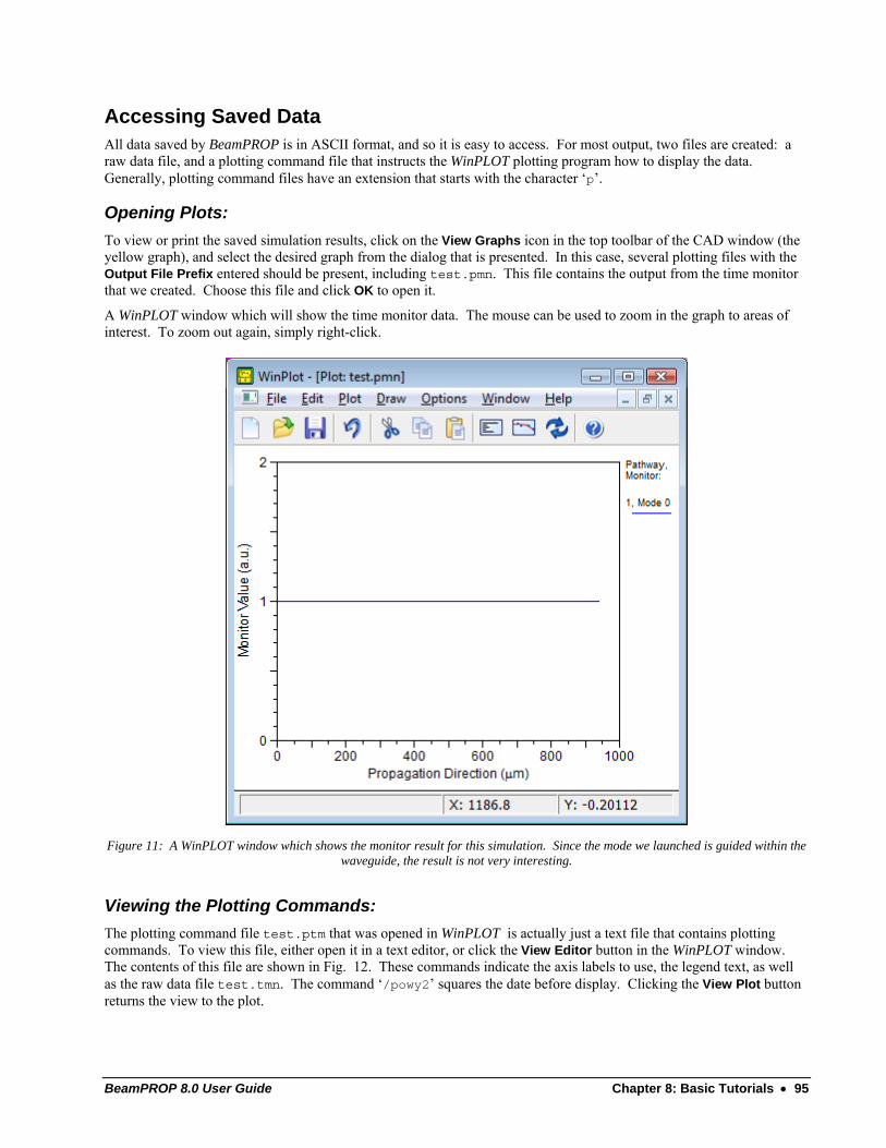
BeamPROP 8.0 User Guide Chapter 8: Basic Tutorials • 95
Accessing Saved Data All data saved by BeamPROP is in ASCII format, and so it is easy to access. For most output, two files are created: a raw data file, and a plotting command file that instructs the WinPLOT plotting program how to display the data. Generally, plotting command files have an extension that starts with the character ‘p’.
Opening Plots: To view or print the saved simulation results, click on the View Graphs icon in the top toolbar of the CAD window (the yellow graph), and select the desired graph from the dialog that is presented. In this case, several plotting files with the Output File Prefix entered should be present, including test.pmn. This file contains the output from the time monitor that we created. Choose this file and click OK to open it.
A WinPLOT window which will show the time monitor data. The mouse can be used to zoom in the graph to areas of interest. To zoom out again, simply right-click.
Figure 11: A WinPLOT window which shows the monitor result for this simulation. Since the mode we launched is guided within the waveguide, the result is not very interesting.
Viewing the Plotting Commands: The plotting command file test.ptm that was opened in WinPLOT is actually just a text file that contains plotting commands. To view this file, either open it in a text editor, or click the View Editor button in the WinPLOT window. The contents of this file are shown in Fig. 12. These commands indicate the axis labels to use, the legend text, as well as the raw data file test.tmn. The command ‘/powy2’ squares the date before display. Clicking the View Plot button returns the view to the plot.
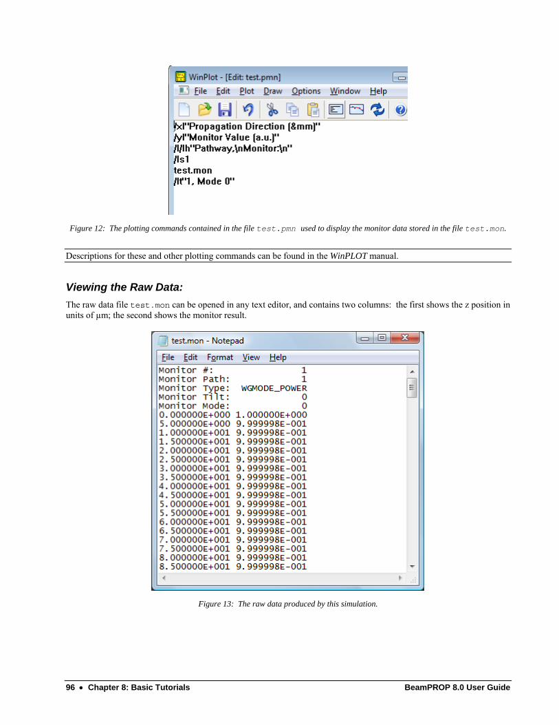
96 • Chapter 8: Basic Tutorials BeamPROP 8.0 User Guide
Figure 12: The plotting commands contained in the file test.pmn used to display the monitor data stored in the file test.mon.
Descriptions for these and other plotting commands can be found in the WinPLOT manual.
Viewing the Raw Data: The raw data file test.mon can be opened in any text editor, and contains two columns: the first shows the z position in units of µm; the second shows the monitor result.
Figure 13: The raw data produced by this simulation.

BeamPROP 8.0 User Guide Chapter 8: Basic Tutorials • 97
Viewing other Types of Output: Most other types of output produced by BeamPROP are controlled by the Output button in the simulation parameters window. A detailed description of the BeamPROP outputs can be found in Section 4.D, and examples of several output types are given in the next tutorials.
Areas for Further Exploration: Several areas to explore include:
• Producing Complex Monitor Plots:
In the above example we used a simple device with no loss. Try creating a simple splitter structure with branches that come out from the waveguide already created. Create pathways and monitors for all the waveguides you add, and rerun the simulation and see how the monitor results change.
• Showing the Structure Outline:
It can be useful to display the structure outline in the simulation window. To do this, open the BeamPROP Simulation Parameters dialog and click the Display… button. Set the Outline Color to Default and click OK twice to perform the simulation. The structure outline will now be displayed in the simulation window.
• Changing the Color Scale
A color scale is used to map the field values displayed during a simulation to particular colors for display. To change the color scale used, open the FullWAVE Simulation Parameters dialog and set the Color Scale field to the desired file. The Scale Files… button can be used to locate the color scale needed. For information regarding the use and creation of color scale files can be found in an Appendix in the CAD manual.

BeamPROP 8.0 User Guide Chapter 8: Basic Tutorials • 99
Basic Tutorial 2: Basic 3D Simulation This tutorial illustrates a basic 3D BeamPROP simulation. Our goal will be to layout and simulate the propagation of a mode at 1.55 µm along a fiber with a cladding index of 1.49, a core index of 1.5, and a diameter of 9 µm.
This tutorial will introduce basic concepts for a 3D simulation. Familiarity with the concepts presented in Basic Tutorial 1 are assumed. If you have not already read through Basic Tutorial 1, please do so now.
3D Specific CAD Options We begin by opening up the RSoft CAD window. Click the New Circuit icon in the top toolbar and make the following settings:
Parameter Value Description
Simulation Tool BeamPROP Indicates that the BeamPROP simulation engine should be used for this simulation.
Model Dimension 3D Indicates that a 3D simulation should be performed.
Free Space Wavelength 1.55 This is the global wavelength (in µm) to be used for the simulation.
Background Index 1.49 This represents the real refractive index of the background material where no structure has been defined.
Index Difference 0.01 This represents the default difference between a component and the background material. In this case this means that the structure will have an index of 1.5. This is simply the default value to be used for a component; each component can have a unique value if desired.
3D Structure Type Fiber This option sets the profile to be used for 3D components. The choice Fiber indicates that, by default, a component should have a circular cross section with a horizontal and vertical diameter given by the Component Width and Component Height fields respectively. By setting these fields equal, a circular cross-section is achieved.
Component Width 9.0 This represents the default width of a component in µm. This is simply the default value to be used for a component; each component can have a unique value if desired.
Component Height width This represents the default height of a component in µm. This is simply the default value to be used for a component; each component can have a unique value if desired. The variable width is the built-in variable which corresponds to the value of the Component Width field.
Once these settings are made, click OK to continue.
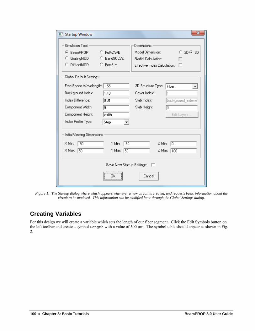
100 • Chapter 8: Basic Tutorials BeamPROP 8.0 User Guide
Figure 1: The Startup dialog where which appears whenever a new circuit is created, and requests basic information about the circuit to be modeled. This information can be modified later through the Global Settings dialog.
Creating Variables For this design we will create a variable which sets the length of our fiber segment. Click the Edit Symbols button on the left toolbar and create a symbol Length with a value of 500 µm. The symbol table should appear as shown in Fig. 2.
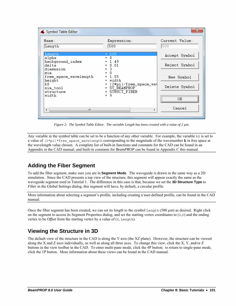
BeamPROP 8.0 User Guide Chapter 8: Basic Tutorials • 101
Figure 2: The Symbol Table Editor. The variable Length has been created with a value of 2 µm.
Any variable in the symbol table can be set to be a function of any other variable. For example, the variable k0 is set to a value of (2*pi)*free_space_wavelength corresponding to the magnitude of the wavenumber k in free space at the wavelength value chosen. A complete list of built-in functions and constants for the CAD can be found in an Appendix in the CAD manual, and built-in constants for BeamPROP can be found in Appendix C this manual.
Adding the Fiber Segment To add the fiber segment, make sure you are in Segment Mode. The waveguide is drawn in the same way as a 2D simulation. Since the CAD presents a top view of the structure, this segment will appear exactly the same as the waveguide segment used in Tutorial 1. The difference in this case is that, because we set the 3D Structure Type to Fiber in the Global Settings dialog, this segment will have, by default, a circular profile.
More information about selecting a segment’s profile, including creating a user-defined profile, can be found in the CAD manual.
Once the fiber segment has been created, we can set its length to the symbol Length (500 µm) as desired. Right click on the segment to access its Segment Properties dialog, and set the starting vertex coordinates to (0,0) and the ending vertex to be Offset from the starting vertex by a value of (0, Length).
Viewing the Structure in 3D The default view of the structure in the CAD is along the Y axis (the XZ plane). However, the structure can be viewed along the X and Z axes individually, as well as along all three axes. To change this view, click the X, Y, and/or Z buttons in the view toolbar in the CAD. To enter multi-pane mode, click the 4P button; to return to single-pane mode, click the 1P button. More information about these views can be found in the CAD manual.
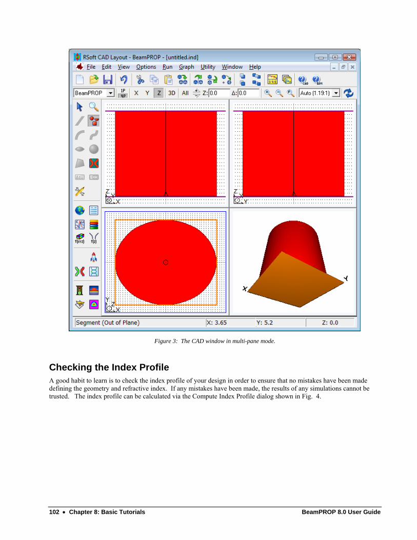
102 • Chapter 8: Basic Tutorials BeamPROP 8.0 User Guide
Figure 3: The CAD window in multi-pane mode.
Checking the Index Profile A good habit to learn is to check the index profile of your design in order to ensure that no mistakes have been made defining the geometry and refractive index. If any mistakes have been made, the results of any simulations cannot be trusted. The index profile can be calculated via the Compute Index Profile dialog shown in Fig. 4.
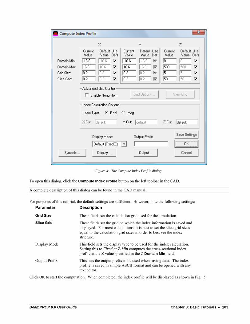
BeamPROP 8.0 User Guide Chapter 8: Basic Tutorials • 103
Figure 4: The Compute Index Profile dialog.
To open this dialog, click the Compute Index Profile button on the left toolbar in the CAD.
A complete description of this dialog can be found in the CAD manual.
For purposes of this tutorial, the default settings are sufficient. However, note the following settings: Parameter Description
Grid Size These fields set the calculation grid used for the simulation.
Slice Grid These fields set the grid on which the index information is saved and displayed. For most calculations, it is best to set the slice grid sizes equal to the calculation grid sizes in order to best see the index stricture.
Display Mode This field sets the display type to be used for the index calculation. Setting this to Fixed at Z-Min computes the cross-sectional index profile at the Z value specified in the Z Domain Min field.
Output Prefix This sets the output prefix to be used when saving data. The index profile is saved in simple ASCII format and can be opened with any text editor.
Click OK to start the computation. When completed, the index profile will be displayed as shown in Fig. 5.
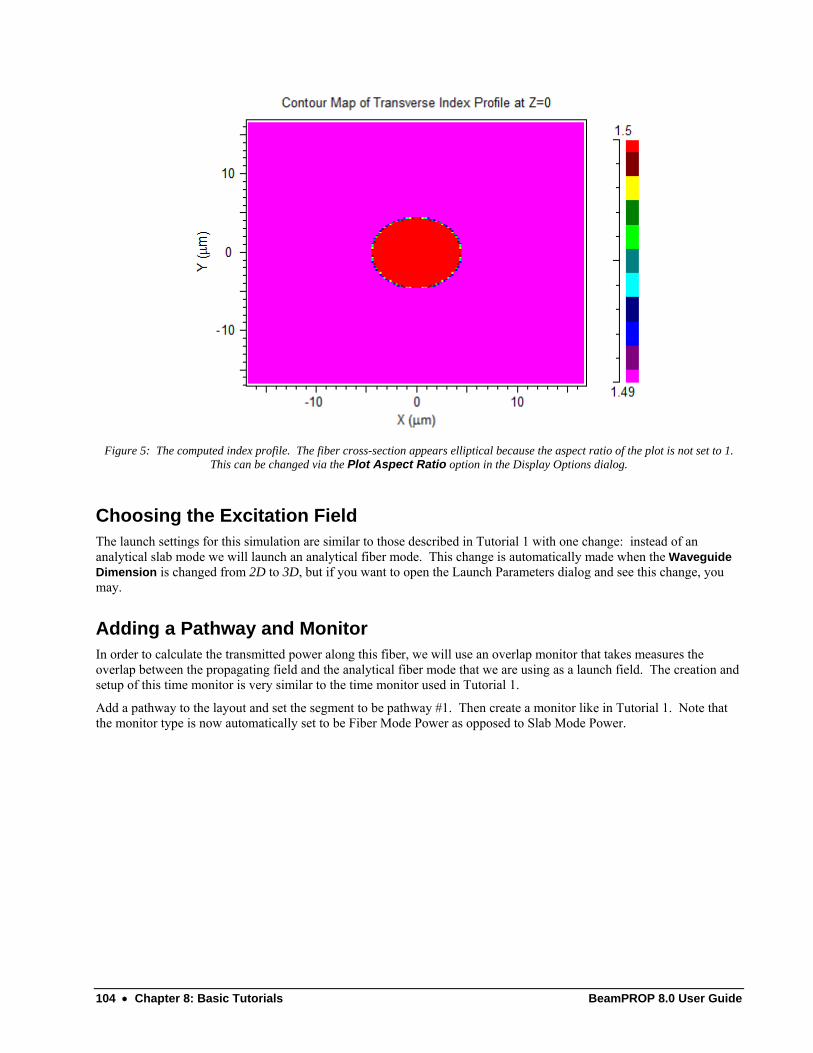
104 • Chapter 8: Basic Tutorials BeamPROP 8.0 User Guide
Figure 5: The computed index profile. The fiber cross-section appears elliptical because the aspect ratio of the plot is not set to 1. This can be changed via the Plot Aspect Ratio option in the Display Options dialog.
Choosing the Excitation Field The launch settings for this simulation are similar to those described in Tutorial 1 with one change: instead of an analytical slab mode we will launch an analytical fiber mode. This change is automatically made when the Waveguide Dimension is changed from 2D to 3D, but if you want to open the Launch Parameters dialog and see this change, you may.
Adding a Pathway and Monitor In order to calculate the transmitted power along this fiber, we will use an overlap monitor that takes measures the overlap between the propagating field and the analytical fiber mode that we are using as a launch field. The creation and setup of this time monitor is very similar to the time monitor used in Tutorial 1.
Add a pathway to the layout and set the segment to be pathway #1. Then create a monitor like in Tutorial 1. Note that the monitor type is now automatically set to be Fiber Mode Power as opposed to Slab Mode Power.
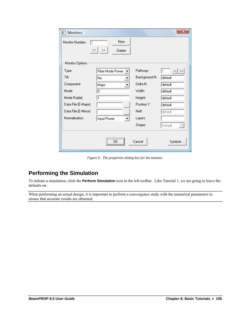
BeamPROP 8.0 User Guide Chapter 8: Basic Tutorials • 105
Figure 6: The properties dialog box for the monitor.
Performing the Simulation To initiate a simulation, click the Perform Simulation icon in the left toolbar. Like Tutorial 1, we are going to leave the defaults on.
When performing an actual design, it is important to perform a convergence study with the numerical parameters to ensure that accurate results are obtained.
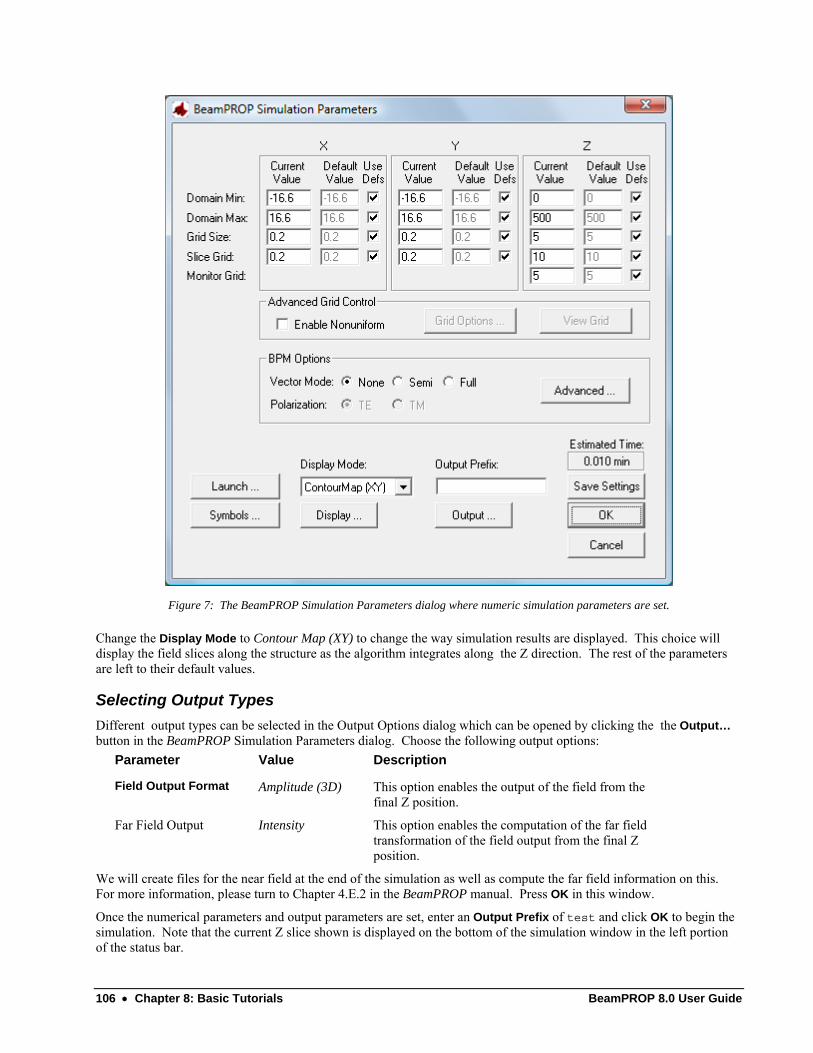
106 • Chapter 8: Basic Tutorials BeamPROP 8.0 User Guide
Figure 7: The BeamPROP Simulation Parameters dialog where numeric simulation parameters are set.
Change the Display Mode to Contour Map (XY) to change the way simulation results are displayed. This choice will display the field slices along the structure as the algorithm integrates along the Z direction. The rest of the parameters are left to their default values.
Selecting Output Types Different output types can be selected in the Output Options dialog which can be opened by clicking the the Output… button in the BeamPROP Simulation Parameters dialog. Choose the following output options: Parameter Value Description
Field Output Format Amplitude (3D) This option enables the output of the field from the final Z position.
Far Field Output Intensity This option enables the computation of the far field transformation of the field output from the final Z position.
We will create files for the near field at the end of the simulation as well as compute the far field information on this. For more information, please turn to Chapter 4.E.2 in the BeamPROP manual. Press OK in this window.
Once the numerical parameters and output parameters are set, enter an Output Prefix of test and click OK to begin the simulation. Note that the current Z slice shown is displayed on the bottom of the simulation window in the left portion of the status bar.
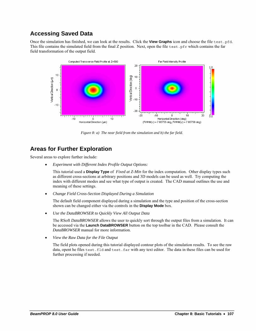
BeamPROP 8.0 User Guide Chapter 8: Basic Tutorials • 107
Accessing Saved Data Once the simulation has finished, we can look at the results. Click the View Graphs icon and choose the file test.pfd. This file contains the simulated field from the final Z position. Next, open the file test.pfr which contains the far field transformation of the output field.
Figure 8: a) The near field from the simulation and b) the far field.
Areas for Further Exploration Several areas to explore further include:
• Experiment with Different Index Profile Output Options:
This tutorial used a Display Type of Fixed at Z-Min for the index computation. Other display types such as different cross-sections at arbitrary positions and 3D models can be used as well. Try computing the index with different modes and see what type of output is created. The CAD manual outlines the use and meaning of these settings.
• Change Field Cross-Section Displayed During a Simulation
The default field component displayed during a simulation and the type and position of the cross-section shown can be changed either via the controls in the Display Mode box.
• Use the DataBROWSER to Quickly View All Output Data
The RSoft DataBROWSER allows the user to quickly sort through the output files from a simulation. It can be accessed via the Launch DataBROWSER button on the top toolbar in the CAD. Please consult the DataBROWSER manual for more information.
• View the Raw Data for the File Output
The field plots opened during this tutorial displayed contour plots of the simulation results. To see the raw data, opent he files test.fld and test.far with any text editor. The data in these files can be used for further processing if needed.

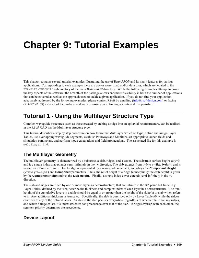
BeamPROP 8.0 User Guide Chapter 9: Tutorial Examples • 109
Chapter 9: Tutorial Examples
This chapter contains several tutorial examples illustrating the use of BeamPROP and its many features for various applications. Corresponding to each example there are one or more .ind and/or data files, which are located in the EXAMPLES\TUTORIAL subdirectory of the main BeamPROP directory. While the following examples attempt to cover the key aspects of the software, the breadth of the package allows enormous flexibility in both the number of applications that can be covered as well as the approach used to tackle a given application. If you do not find your application adequately addressed by the following examples, please contact RSoft by emailing ([email protected]) or faxing (914-923-2169) a sketch of the problem and we will assist you in finding a solution if it is possible.
Tutorial 1 - Using the Multilayer Structure Type Complex waveguide structures, such as those created by etching a ridge into an epitaxial heterostructure, can be realized in the RSoft CAD via the Multilayer structure type.
This tutorial describes a step by step procedure on how to use the Multilayer Structure Type, define and assign Layer Tables, use overlapping waveguide segments, establish Pathways and Monitors, set appropriate launch fields and simulation parameters, and perform mode calculations and field propagations. The associated file for this example is multilayer.ind.
The Multilayer Geometry The multilayer geometry is characterized by a substrate, a slab, ridges, and a cover. The substrate surface begins at y=0, and is a single index that extends semi-infinitely in the –y direction. The slab extends from y=0 to y=Slab Height, and is treated as infinite in x and z. Each ridge is represented by a waveguide segement, and obeys the Component Height (y=0 to y=height) and Componentparameters. Thus, the relief height of a ridge (conceptually the etch depth) is given by the Component Height minus the Slab Height. Finally, a single index cover extends semi-infinitely in the +y direction.
The slab and ridges are filled by one or more layers (a heterostructure) that are infinite in the XZ plane but finite in y. Layer Tables, defined by the user, describe the thickness and complex index of each layer in a heterostructure. The total height of the cumulative layers in a table should be equal to or greater than the height of the ridge(s) or slab which refers to it. Any additional thickness is truncated. Specifically, the slab is described only by Layer Table #0, while the ridges can refer to any of the defined tables. As stated, the slab persists everywhere regardless of whether there are any ridges, and where a ridge exists, it’s index structure has precedence over that of the slab. If ridges overlap with each other, the segment priority determines the precedence.
Device Layout
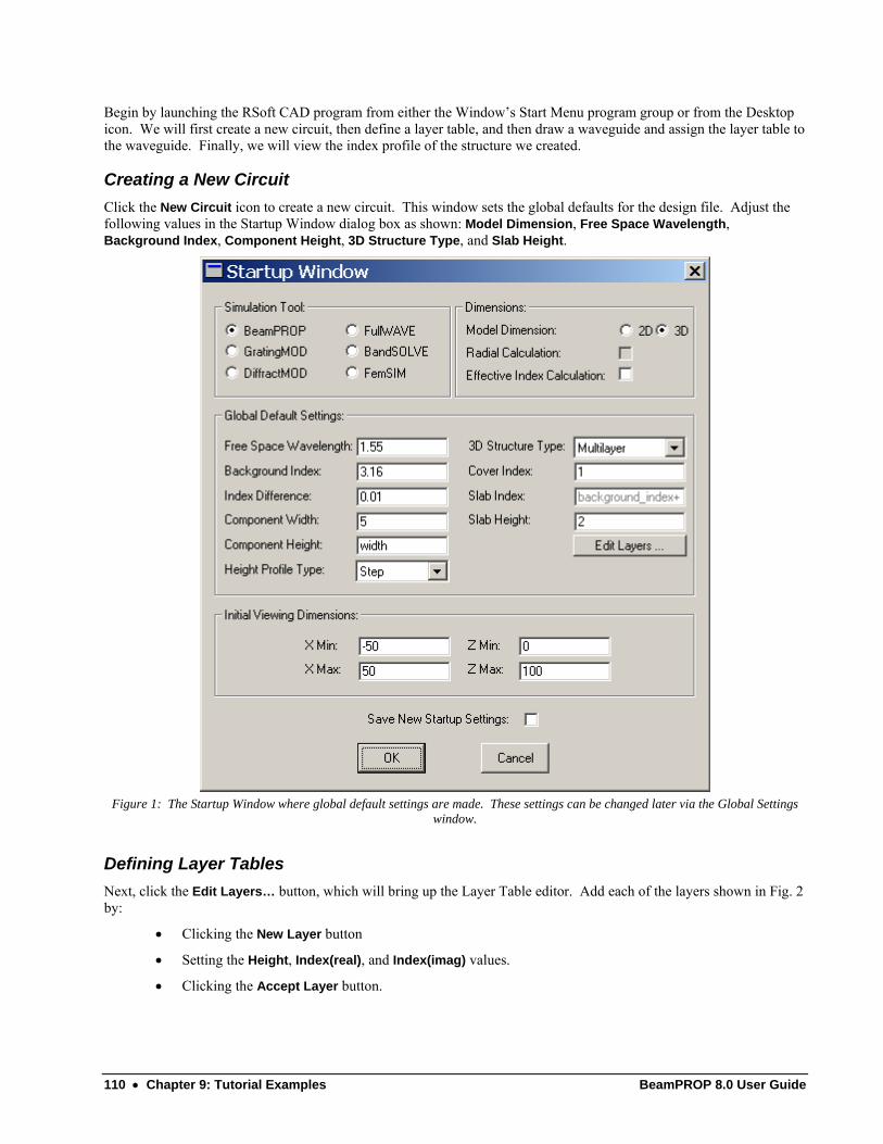
110 • Chapter 9: Tutorial Examples BeamPROP 8.0 User Guide
Begin by launching the RSoft CAD program from either the Window’s Start Menu program group or from the Desktop icon. We will first create a new circuit, then define a layer table, and then draw a waveguide and assign the layer table to the waveguide. Finally, we will view the index profile of the structure we created.
Creating a New Circuit Click the New Circuit icon to create a new circuit. This window sets the global defaults for the design file. Adjust the following values in the Startup Window dialog box as shown: Model Dimension, Free Space Wavelength, Background Index, Component Height, 3D Structure Type, and Slab Height.
Figure 1: The Startup Window where global default settings are made. These settings can be changed later via the Global Settings
window.
Defining Layer Tables Next, click the Edit Layers… button, which will bring up the Layer Table editor. Add each of the layers shown in Fig. 2 by:
• Clicking the New Layer button
• Setting the Height, Index(real), and Index(imag) values.
• Clicking the Accept Layer button.
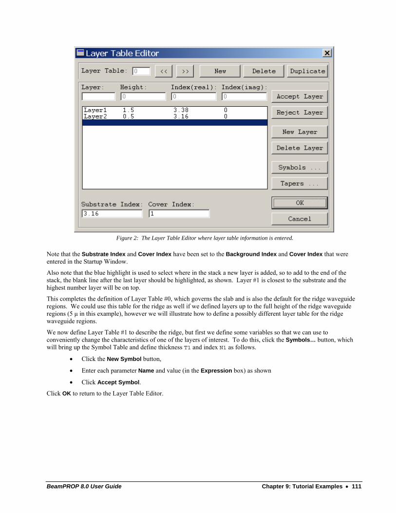
BeamPROP 8.0 User Guide Chapter 9: Tutorial Examples • 111
Figure 2: The Layer Table Editor where layer table information is entered.
Note that the Substrate Index and Cover Index have been set to the Background Index and Cover Index that were entered in the Startup Window.
Also note that the blue highlight is used to select where in the stack a new layer is added, so to add to the end of the stack, the blank line after the last layer should be highlighted, as shown. Layer #1 is closest to the substrate and the highest number layer will be on top.
This completes the definition of Layer Table #0, which governs the slab and is also the default for the ridge waveguide regions. We could use this table for the ridge as well if we defined layers up to the full height of the ridge waveguide regions (5 μ in this example), however we will illustrate how to define a possibly different layer table for the ridge waveguide regions.
We now define Layer Table #1 to describe the ridge, but first we define some variables so that we can use to conveniently change the characteristics of one of the layers of interest. To do this, click the Symbols… button, which will bring up the Symbol Table and define thickness T1 and index N1 as follows.
• Click the New Symbol button,
• Enter each parameter Name and value (in the Expression box) as shown
• Click Accept Symbol.
Click OK to return to the Layer Table Editor.
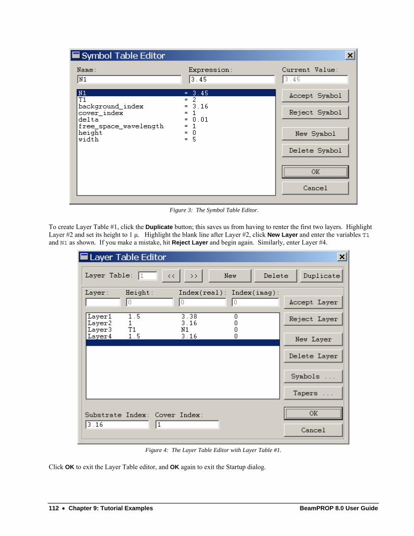
112 • Chapter 9: Tutorial Examples BeamPROP 8.0 User Guide
Figure 3: The Symbol Table Editor.
To create Layer Table #1, click the Duplicate button; this saves us from having to renter the first two layers. Highlight Layer #2 and set its height to 1 μ. Highlight the blank line after Layer #2, click New Layer and enter the variables T1 and N1 as shown. If you make a mistake, hit Reject Layer and begin again. Similarly, enter Layer #4.
Figure 4: The Layer Table Editor with Layer Table #1.
Click OK to exit the Layer Table editor, and OK again to exit the Startup dialog.
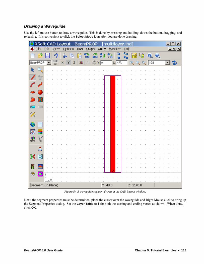
BeamPROP 8.0 User Guide Chapter 9: Tutorial Examples • 113
Drawing a Waveguide Use the left mouse button to draw a waveguide. This is done by pressing and holding down the button, dragging, and releasing. It is convenient to click the Select Mode icon after you are done drawing.
Figure 5: A waveguide segment drawn in the CAD Layout window.
Next, the segment properties must be determined; place the cursor over the waveguide and Right Mouse click to bring up the Segment Properties dialog. Set the Layer Table to 1 for both the starting and ending vertex as shown. When done, click OK.
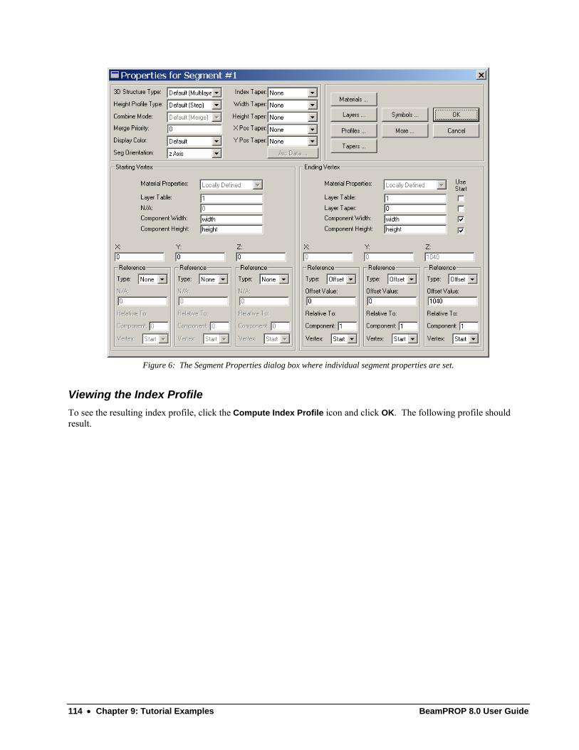
114 • Chapter 9: Tutorial Examples BeamPROP 8.0 User Guide
Figure 6: The Segment Properties dialog box where individual segment properties are set.
Viewing the Index Profile To see the resulting index profile, click the Compute Index Profile icon and click OK. The following profile should result.
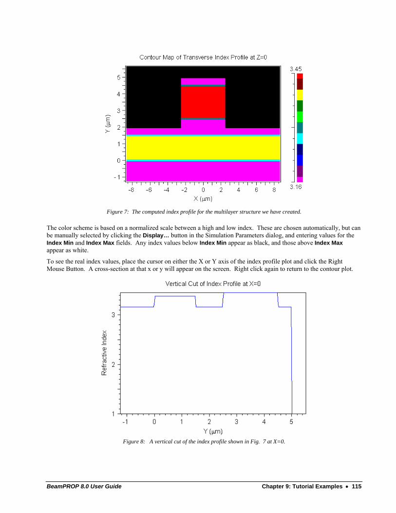
BeamPROP 8.0 User Guide Chapter 9: Tutorial Examples • 115
Figure 7: The computed index profile for the multilayer structure we have created.
The color scheme is based on a normalized scale between a high and low index. These are chosen automatically, but can be manually selected by clicking the Display… button in the Simulation Parameters dialog, and entering values for the Index Min and Index Max fields. Any index values below Index Min appear as black, and those above Index Max appear as white.
To see the real index values, place the cursor on either the X or Y axis of the index profile plot and click the Right Mouse Button. A cross-section at that x or y will appear on the screen. Right click again to return to the contour plot.
Figure 8: A vertical cut of the index profile shown in Fig. 7 at X=0.
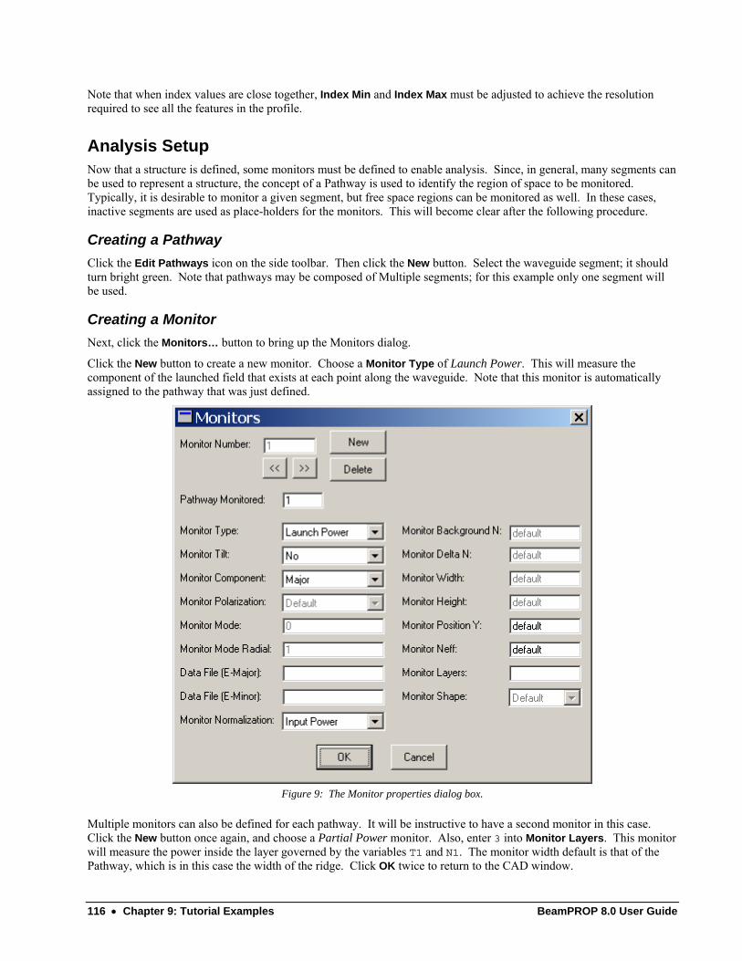
116 • Chapter 9: Tutorial Examples BeamPROP 8.0 User Guide
Note that when index values are close together, Index Min and Index Max must be adjusted to achieve the resolution required to see all the features in the profile.
Analysis Setup Now that a structure is defined, some monitors must be defined to enable analysis. Since, in general, many segments can be used to represent a structure, the concept of a Pathway is used to identify the region of space to be monitored. Typically, it is desirable to monitor a given segment, but free space regions can be monitored as well. In these cases, inactive segments are used as place-holders for the monitors. This will become clear after the following procedure.
Creating a Pathway Click the Edit Pathways icon on the side toolbar. Then click the New button. Select the waveguide segment; it should turn bright green. Note that pathways may be composed of Multiple segments; for this example only one segment will be used.
Creating a Monitor Next, click the Monitors… button to bring up the Monitors dialog.
Click the New button to create a new monitor. Choose a Monitor Type of Launch Power. This will measure the component of the launched field that exists at each point along the waveguide. Note that this monitor is automatically assigned to the pathway that was just defined.
Figure 9: The Monitor properties dialog box.
Multiple monitors can also be defined for each pathway. It will be instructive to have a second monitor in this case. Click the New button once again, and choose a Partial Power monitor. Also, enter 3 into Monitor Layers. This monitor will measure the power inside the layer governed by the variables T1 and N1. The monitor width default is that of the Pathway, which is in this case the width of the ridge. Click OK twice to return to the CAD window.
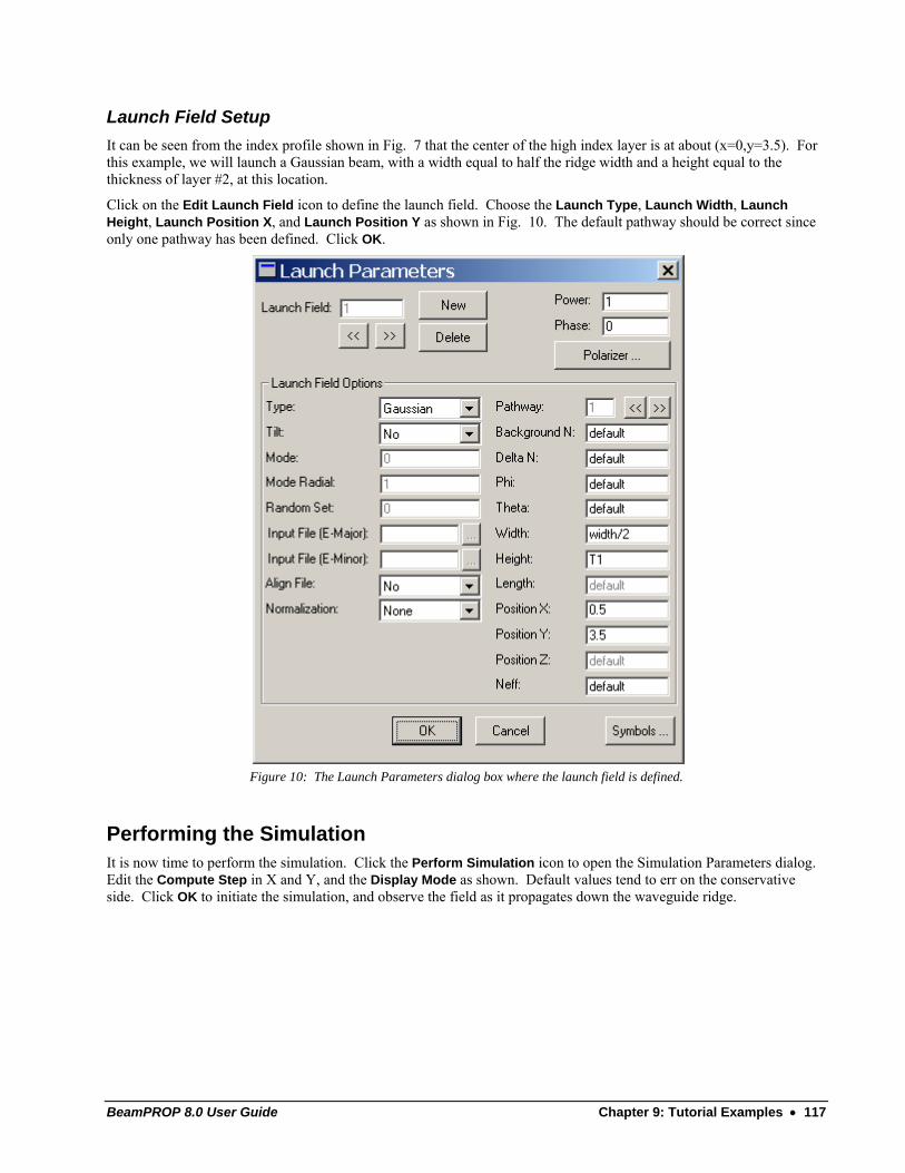
BeamPROP 8.0 User Guide Chapter 9: Tutorial Examples • 117
Launch Field Setup It can be seen from the index profile shown in Fig. 7 that the center of the high index layer is at about (x=0,y=3.5). For this example, we will launch a Gaussian beam, with a width equal to half the ridge width and a height equal to the thickness of layer #2, at this location.
Click on the Edit Launch Field icon to define the launch field. Choose the Launch Type, Launch Width, Launch Height, Launch Position X, and Launch Position Y as shown in Fig. 10. The default pathway should be correct since only one pathway has been defined. Click OK.
Figure 10: The Launch Parameters dialog box where the launch field is defined.
Performing the Simulation It is now time to perform the simulation. Click the Perform Simulation icon to open the Simulation Parameters dialog. Edit the Compute Step in X and Y, and the Display Mode as shown. Default values tend to err on the conservative side. Click OK to initiate the simulation, and observe the field as it propagates down the waveguide ridge.
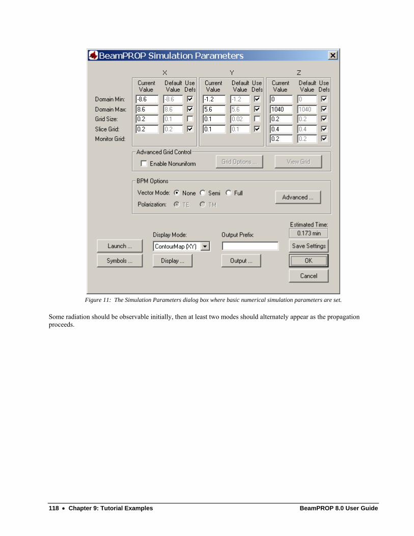
118 • Chapter 9: Tutorial Examples BeamPROP 8.0 User Guide
Figure 11: The Simulation Parameters dialog box where basic numerical simulation parameters are set.
Some radiation should be observable initially, then at least two modes should alternately appear as the propagation proceeds.
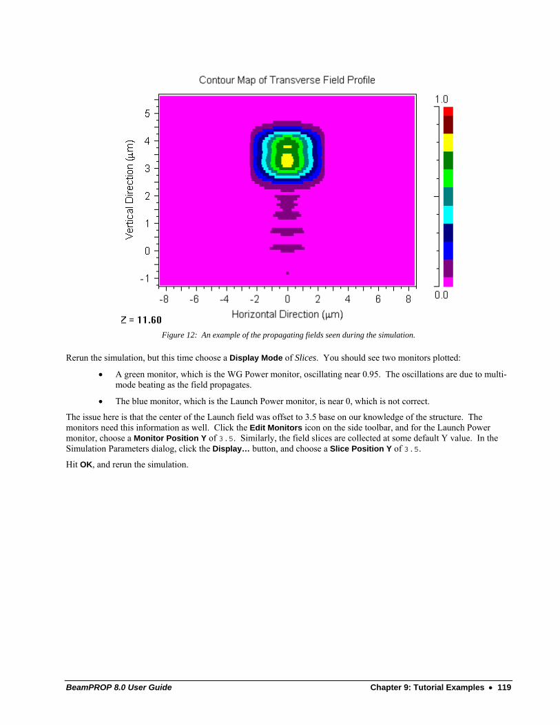
BeamPROP 8.0 User Guide Chapter 9: Tutorial Examples • 119
Figure 12: An example of the propagating fields seen during the simulation.
Rerun the simulation, but this time choose a Display Mode of Slices. You should see two monitors plotted:
• A green monitor, which is the WG Power monitor, oscillating near 0.95. The oscillations are due to multi-mode beating as the field propagates.
• The blue monitor, which is the Launch Power monitor, is near 0, which is not correct.
The issue here is that the center of the Launch field was offset to 3.5 base on our knowledge of the structure. The monitors need this information as well. Click the Edit Monitors icon on the side toolbar, and for the Launch Power monitor, choose a Monitor Position Y of 3.5. Similarly, the field slices are collected at some default Y value. In the Simulation Parameters dialog, click the Display… button, and choose a Slice Position Y of 3.5.
Hit OK, and rerun the simulation.
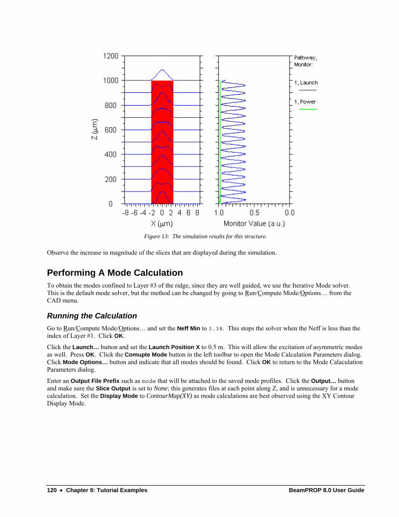
120 • Chapter 9: Tutorial Examples BeamPROP 8.0 User Guide
Figure 13: The simulation results for this structure.
Observe the increase in magnitude of the slices that are displayed during the simulation.
Performing A Mode Calculation To obtain the modes confined to Layer #3 of the ridge, since they are well guided, we use the Iterative Mode solver. This is the default mode solver, but the method can be changed by going to Run/Compute Mode/Options… from the CAD menu.
Running the Calculation Go to Run/Compute Mode/Options… and set the Neff Min to 3.38. This stops the solver when the Neff is less than the index of Layer #1. Click OK.
Click the Launch… button and set the Launch Position X to 0.5 m. This will allow the excitation of asymmetric modes as well. Press OK. Click the Comupte Mode button in the left toolbar to open the Mode Calculation Parameters dialog. Click Mode Options… button and indicate that all modes should be found. Click OK to return to the Mode Calaculation Parameters dialog.
Enter an Output File Prefix such as mode that will be attached to the saved mode profiles. Click the Output… button and make sure the Slice Output is set to None; this generates files at each point along Z, and is unnecessary for a mode calculation. Set the Display Mode to ContourMap(XY) as mode calculations are best observed using the XY Contour Display Mode.

BeamPROP 8.0 User Guide Chapter 9: Tutorial Examples • 121
Figure 14: The Simulation Parameters for the mode calculation.
Click OK in the Simulation Parameters dialog box to run the mode solver.
Note that if the waveguide segment is not long enough to allow convergence, a warning message will occur when the propagation reaches the end of the pathway. This can be simply fixed by lengthening the structure.
Accessing the Calculated Modes The resulting modes can be seen by pressing the View Graphs icon on the top of the screen and selecting the files that begin with the Output File Prefix given, or mode. The modes look like the following:
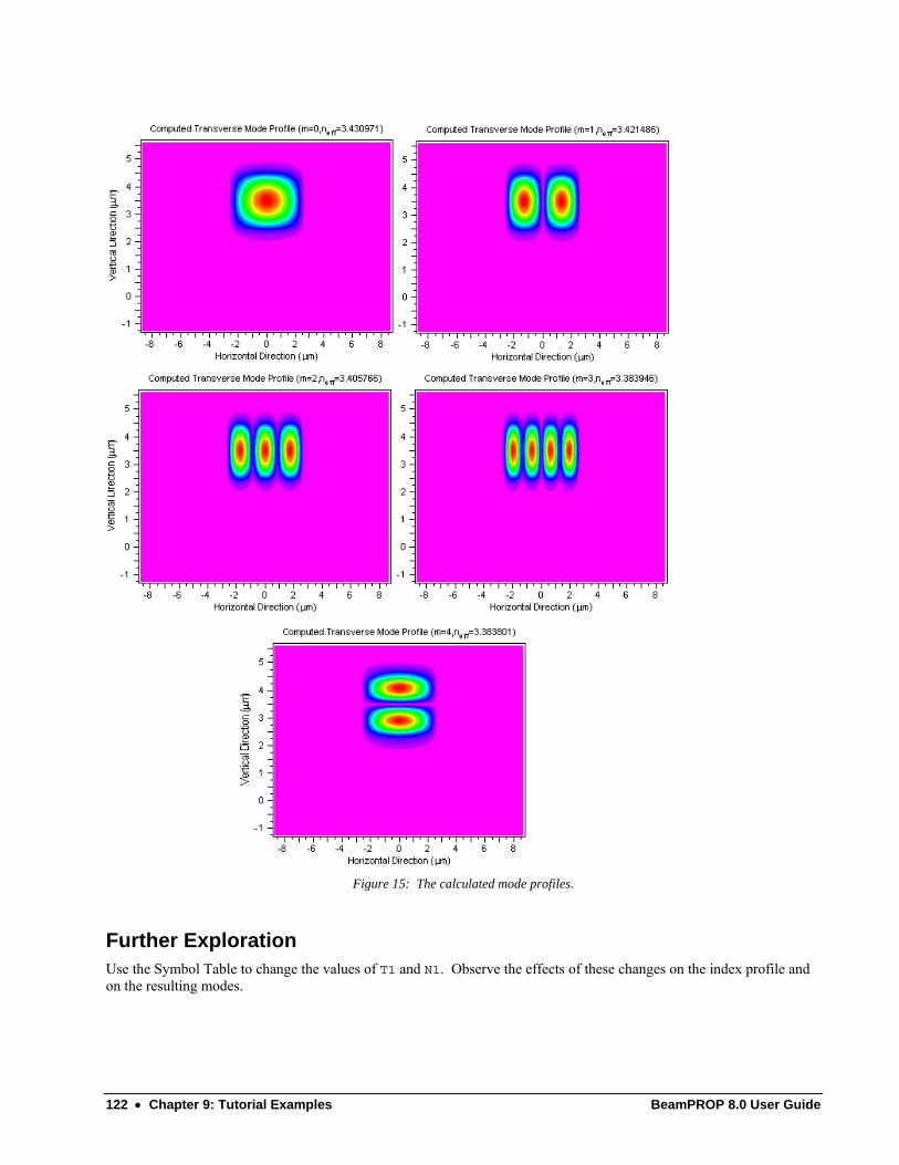
122 • Chapter 9: Tutorial Examples BeamPROP 8.0 User Guide
Figure 15: The calculated mode profiles.
Further Exploration Use the Symbol Table to change the values of T1 and N1. Observe the effects of these changes on the index profile and on the resulting modes.
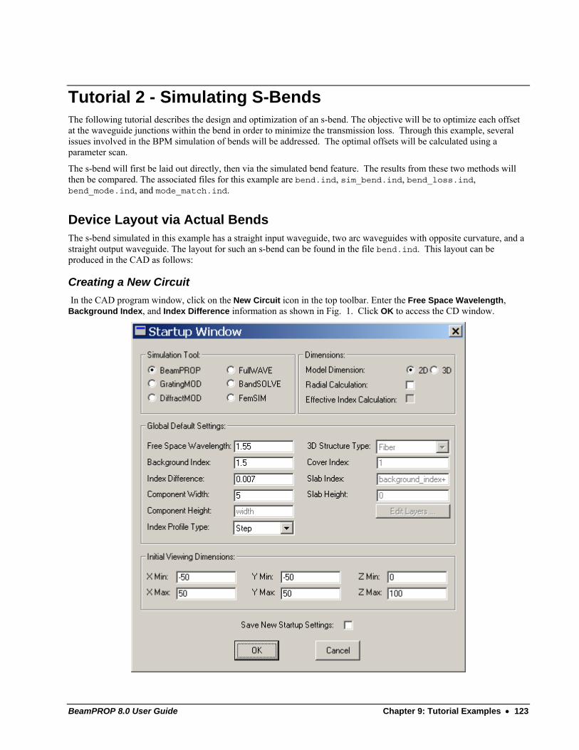
BeamPROP 8.0 User Guide Chapter 9: Tutorial Examples • 123
Tutorial 2 - Simulating S-Bends The following tutorial describes the design and optimization of an s-bend. The objective will be to optimize each offset at the waveguide junctions within the bend in order to minimize the transmission loss. Through this example, several issues involved in the BPM simulation of bends will be addressed. The optimal offsets will be calculated using a parameter scan.
The s-bend will first be laid out directly, then via the simulated bend feature. The results from these two methods will then be compared. The associated files for this example are bend.ind, sim_bend.ind, bend_loss.ind, bend_mode.ind, and mode_match.ind.
Device Layout via Actual Bends The s-bend simulated in this example has a straight input waveguide, two arc waveguides with opposite curvature, and a straight output waveguide. The layout for such an s-bend can be found in the file bend.ind. This layout can be produced in the CAD as follows:
Creating a New Circuit In the CAD program window, click on the New Circuit icon in the top toolbar. Enter the Free Space Wavelength, Background Index, and Index Difference information as shown in Fig. 1. Click OK to access the CD window.
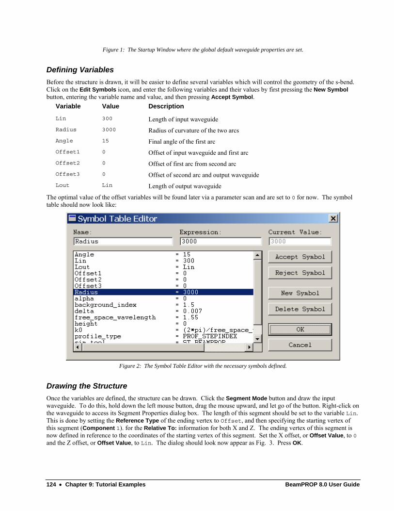
124 • Chapter 9: Tutorial Examples BeamPROP 8.0 User Guide
Figure 1: The Startup Window where the global default waveguide properties are set.
Defining Variables Before the structure is drawn, it will be easier to define several variables which will control the geometry of the s-bend. Click on the Edit Symbols icon, and enter the following variables and their values by first pressing the New Symbol button, entering the variable name and value, and then pressing Accept Symbol. Variable Value Description Lin 300 Length of input waveguide Radius 3000 Radius of curvature of the two arcs Angle 15 Final angle of the first arc Offset1 0 Offset of input waveguide and first arc Offset2 0 Offset of first arc from second arc Offset3 0 Offset of second arc and output waveguide Lout Lin Length of output waveguide
The optimal value of the offset variables will be found later via a parameter scan and are set to 0 for now. The symbol table should now look like:
Figure 2: The Symbol Table Editor with the necessary symbols defined.
Drawing the Structure Once the variables are defined, the structure can be drawn. Click the Segment Mode button and draw the input waveguide. To do this, hold down the left mouse button, drag the mouse upward, and let go of the button. Right-click on the waveguide to access its Segment Properties dialog box. The length of this segment should be set to the variable Lin. This is done by setting the Reference Type of the ending vertex to Offset, and then specifying the starting vertex of this segment (Component 1). for the Relative To: information for both X and Z. The ending vertex of this segment is now defined in reference to the coordinates of the starting vertex of this segment. Set the X offset, or Offset Value, to 0 and the Z offset, or Offset Value, to Lin. The dialog should look now appear as Fig. 3. Press OK.
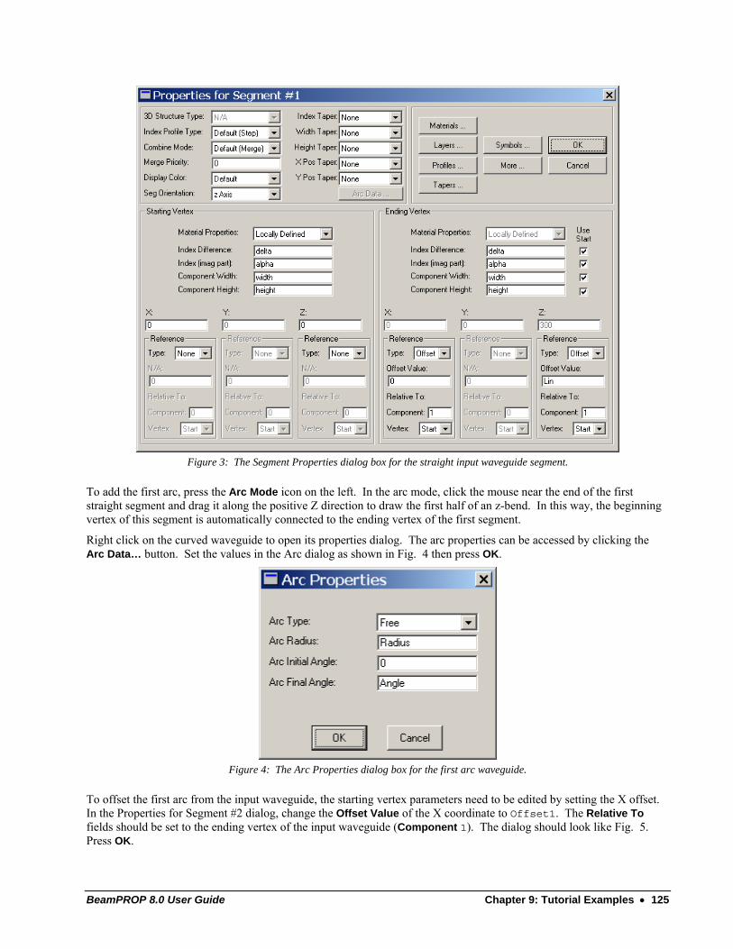
BeamPROP 8.0 User Guide Chapter 9: Tutorial Examples • 125
Figure 3: The Segment Properties dialog box for the straight input waveguide segment.
To add the first arc, press the Arc Mode icon on the left. In the arc mode, click the mouse near the end of the first straight segment and drag it along the positive Z direction to draw the first half of an z-bend. In this way, the beginning vertex of this segment is automatically connected to the ending vertex of the first segment.
Right click on the curved waveguide to open its properties dialog. The arc properties can be accessed by clicking the Arc Data… button. Set the values in the Arc dialog as shown in Fig. 4 then press OK.
Figure 4: The Arc Properties dialog box for the first arc waveguide.
To offset the first arc from the input waveguide, the starting vertex parameters need to be edited by setting the X offset. In the Properties for Segment #2 dialog, change the Offset Value of the X coordinate to Offset1. The Relative To fields should be set to the ending vertex of the input waveguide (Component 1). The dialog should look like Fig. 5. Press OK.
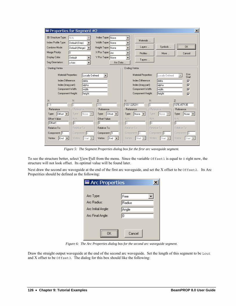
126 • Chapter 9: Tutorial Examples BeamPROP 8.0 User Guide
Figure 5: The Segment Properties dialog box for the firsr arc waveguide segment.
To see the structure better, select View/Full from the menu. Since the variable Offset1 is equal to 0 right now, the structure will not look offset. Its optimal value will be found later.
Next draw the second arc waveguide at the end of the first arc waveguide, and set the X offset to be Offset2. Its Arc Properities should be defined as the following:
Figure 6: The Arc Properties dialog bos for the second arc waveguide segment.
Draw the straight output waveguide at the end of the second arc waveguide. Set the length of this segment to be Lout and X offset to be Offset3. The dialog for this box should like the following:
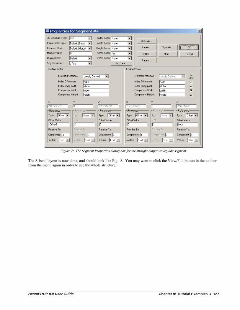
BeamPROP 8.0 User Guide Chapter 9: Tutorial Examples • 127
Figure 7: The Segment Properties dialog box for the straight output waveguide segment.
The S-bend layout is now done, and should look like Fig. 8. You may want to click the View/Full button in the toolbar from the menu again in order to see the whole structure.
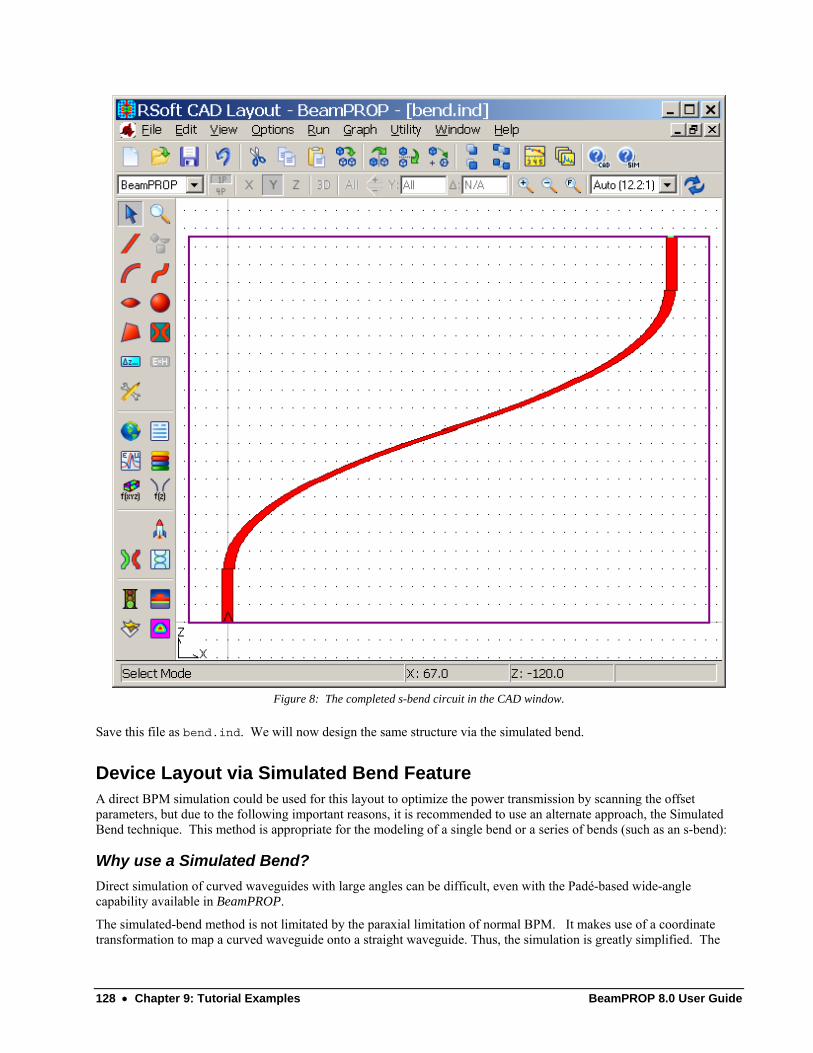
128 • Chapter 9: Tutorial Examples BeamPROP 8.0 User Guide
Figure 8: The completed s-bend circuit in the CAD window.
Save this file as bend.ind. We will now design the same structure via the simulated bend.
Device Layout via Simulated Bend Feature A direct BPM simulation could be used for this layout to optimize the power transmission by scanning the offset parameters, but due to the following important reasons, it is recommended to use an alternate approach, the Simulated Bend technique. This method is appropriate for the modeling of a single bend or a series of bends (such as an s-bend):
Why use a Simulated Bend? Direct simulation of curved waveguides with large angles can be difficult, even with the Padé-based wide-angle capability available in BeamPROP.
The simulated-bend method is not limitated by the paraxial limitation of normal BPM. It makes use of a coordinate transformation to map a curved waveguide onto a straight waveguide. Thus, the simulation is greatly simplified. The
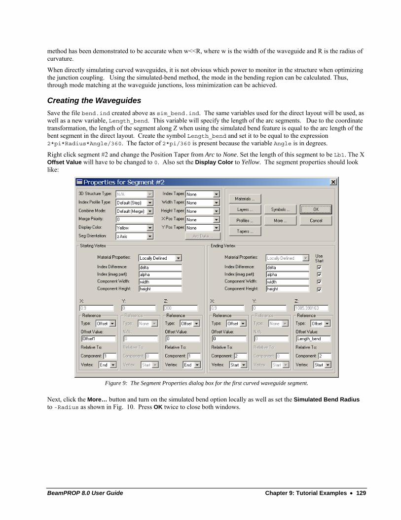
BeamPROP 8.0 User Guide Chapter 9: Tutorial Examples • 129
method has been demonstrated to be accurate when w<<R, where w is the width of the waveguide and R is the radius of curvature.
When directly simulating curved waveguides, it is not obvious which power to monitor in the structure when optimizing the junction coupling. Using the simulated-bend method, the mode in the bending region can be calculated. Thus, through mode matching at the waveguide junctions, loss minimization can be achieved.
Creating the Waveguides Save the file bend.ind created above as sim_bend.ind. The same variables used for the direct layout will be used, as well as a new variable, Length_bend. This variable will specify the length of the arc segments. Due to the coordinate transformation, the length of the segment along Z when using the simulated bend feature is equal to the arc length of the bent segment in the direct layout. Create the symbol Length_bend and set it to be equal to the expression 2*pi*Radius*Angle/360. The factor of 2*pi/360 is present because the variable Angle is in degrees.
Right click segment #2 and change the Position Taper from Arc to None. Set the length of this segment to be Lb1. The X Offset Value will have to be changed to 0. Also set the Display Color to Yellow. The segment properties should look like:
Figure 9: The Segment Properties dialog box for the first curved waveguide segment.
Next, click the More… button and turn on the simulated bend option locally as well as set the Simulated Bend Radius to -Radius as shown in Fig. 10. Press OK twice to close both windows.
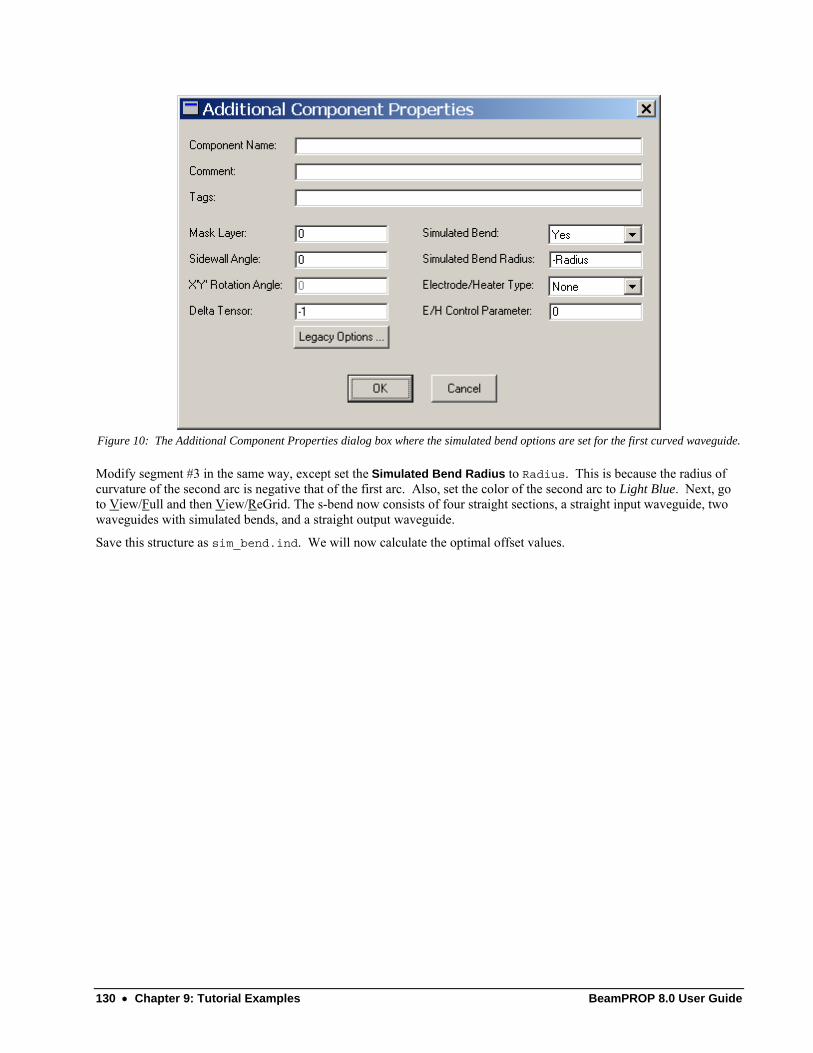
130 • Chapter 9: Tutorial Examples BeamPROP 8.0 User Guide
Figure 10: The Additional Component Properties dialog box where the simulated bend options are set for the first curved waveguide.
Modify segment #3 in the same way, except set the Simulated Bend Radius to Radius. This is because the radius of curvature of the second arc is negative that of the first arc. Also, set the color of the second arc to Light Blue. Next, go to View/Full and then View/ReGrid. The s-bend now consists of four straight sections, a straight input waveguide, two waveguides with simulated bends, and a straight output waveguide.
Save this structure as sim_bend.ind. We will now calculate the optimal offset values.
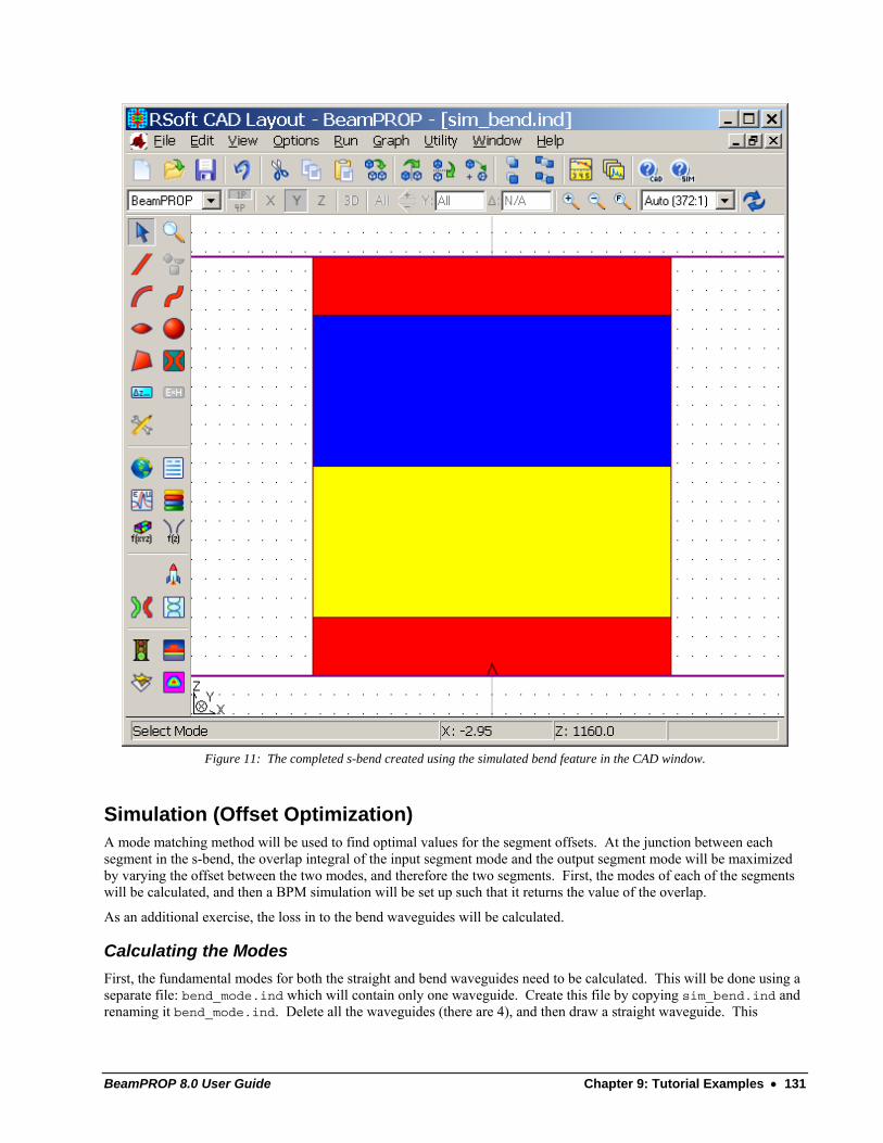
BeamPROP 8.0 User Guide Chapter 9: Tutorial Examples • 131
Figure 11: The completed s-bend created using the simulated bend feature in the CAD window.
Simulation (Offset Optimization) A mode matching method will be used to find optimal values for the segment offsets. At the junction between each segment in the s-bend, the overlap integral of the input segment mode and the output segment mode will be maximized by varying the offset between the two modes, and therefore the two segments. First, the modes of each of the segments will be calculated, and then a BPM simulation will be set up such that it returns the value of the overlap.
As an additional exercise, the loss in to the bend waveguides will be calculated.
Calculating the Modes First, the fundamental modes for both the straight and bend waveguides need to be calculated. This will be done using a separate file: bend_mode.ind which will contain only one waveguide. Create this file by copying sim_bend.ind and renaming it bend_mode.ind. Delete all the waveguides (there are 4), and then draw a straight waveguide. This
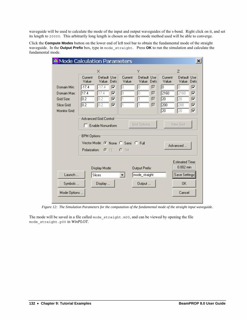
132 • Chapter 9: Tutorial Examples BeamPROP 8.0 User Guide
waveguide will be used to calculate the mode of the input and output waveguides of the s-bend. Right click on it, and set its length to 20000. This arbitrarily long length is chosen so that the mode method used will be able to converge.
Click the Compute Modes button on the lower end of left tool bar to obtain the fundamental mode of the straight waveguide. In the Output Prefix box, type in mode_straight. Press OK to run the simulation and calculate the fundamental mode.
Figure 12: The Simulation Parameters for the computation of the fundamental mode of the straight input waveguide.
The mode will be saved in a file called mode_straight.m00, and can be viewed by opening the file mode_straight.p00 in WinPLOT.
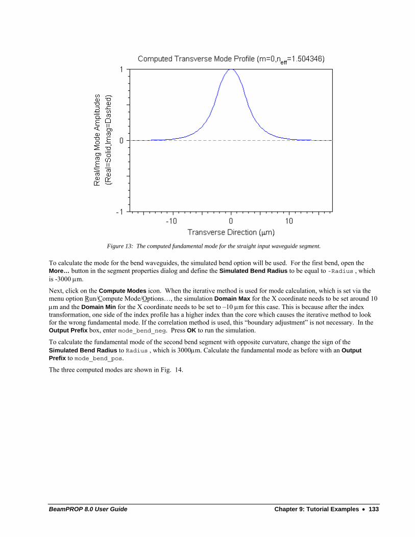
BeamPROP 8.0 User Guide Chapter 9: Tutorial Examples • 133
Figure 13: The computed fundamental mode for the straight input waveguide segment.
To calculate the mode for the bend waveguides, the simulated bend option will be used. For the first bend, open the More… button in the segment properties dialog and define the Simulated Bend Radius to be equal to -Radius , which is -3000 μm.
Next, click on the Compute Modes icon. When the iterative method is used for mode calculation, which is set via the menu option Run/Compute Mode/Options…, the simulation Domain Max for the X coordinate needs to be set around 10 μm and the Domain Min for the X coordinate needs to be set to –10 μm for this case. This is because after the index transformation, one side of the index profile has a higher index than the core which causes the iterative method to look for the wrong fundamental mode. If the correlation method is used, this “boundary adjustment” is not necessary. In the Output Prefix box, enter mode_bend_neg. Press OK to run the simulation.
To calculate the fundamental mode of the second bend segment with opposite curvature, change the sign of the Simulated Bend Radius to Radius , which is 3000μm. Calculate the fundamental mode as before with an Output Prefix to mode_bend_pos.
The three computed modes are shown in Fig. 14.
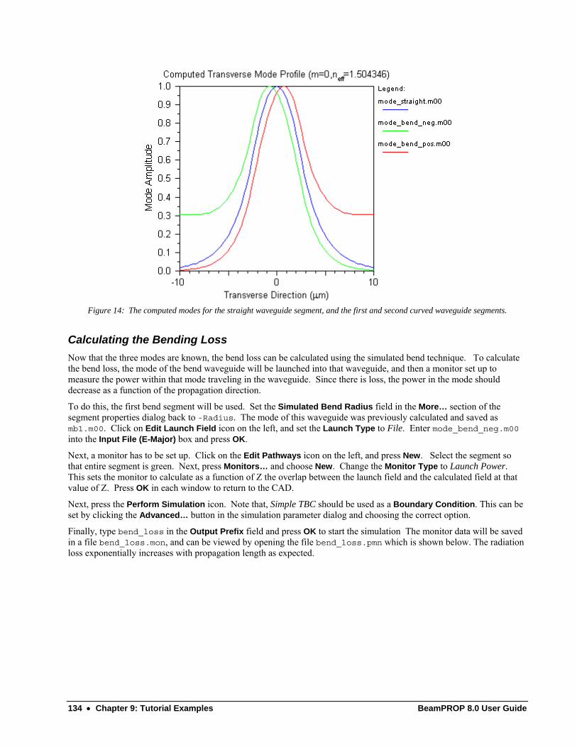
134 • Chapter 9: Tutorial Examples BeamPROP 8.0 User Guide
Figure 14: The computed modes for the straight waveguide segment, and the first and second curved waveguide segments.
Calculating the Bending Loss Now that the three modes are known, the bend loss can be calculated using the simulated bend technique. To calculate the bend loss, the mode of the bend waveguide will be launched into that waveguide, and then a monitor set up to measure the power within that mode traveling in the waveguide. Since there is loss, the power in the mode should decrease as a function of the propagation direction.
To do this, the first bend segment will be used. Set the Simulated Bend Radius field in the More… section of the segment properties dialog back to -Radius. The mode of this waveguide was previously calculated and saved as mb1.m00. Click on Edit Launch Field icon on the left, and set the Launch Type to File. Enter mode_bend_neg.m00 into the Input File (E-Major) box and press OK.
Next, a monitor has to be set up. Click on the Edit Pathways icon on the left, and press New. Select the segment so that entire segment is green. Next, press Monitors… and choose New. Change the Monitor Type to Launch Power. This sets the monitor to calculate as a function of Z the overlap between the launch field and the calculated field at that value of Z. Press OK in each window to return to the CAD.
Next, press the Perform Simulation icon. Note that, Simple TBC should be used as a Boundary Condition. This can be set by clicking the Advanced… button in the simulation parameter dialog and choosing the correct option.
Finally, type bend_loss in the Output Prefix field and press OK to start the simulation The monitor data will be saved in a file bend_loss.mon, and can be viewed by opening the file bend_loss.pmn which is shown below. The radiation loss exponentially increases with propagation length as expected.
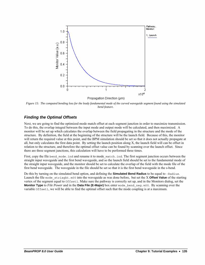
BeamPROP 8.0 User Guide Chapter 9: Tutorial Examples • 135
Figure 15: The computed bending loss for the leady fundamental mode of the curved waveguide segment found using the simulated
bend feature.
Finding the Optimal Offsets Next, we are going to find the optimized mode match offset at each segment junction in order to maximize transmission. To do this, the overlap integral between the input mode and output mode will be calculated, and then maximized. A monitor will be set up which calculates the overlap between the field propagating in the structure and the mode of the structure. By definition, the field at the beginning of the structure will be the launch field. Because of this, the monitor will return the required value at this point, and the BPM simulation should be set so that it does not actually propagate at all, but only calculates the first data point. By setting the launch position along X, the launch field will can be offset in relation to the structure, and therefore the optimal offset value can be found by scanning over the launch offset. Since there are three segment junctions, this calculation will have to be performed three times.
First, copy the file bend_mode.ind and rename it to mode_match.ind. The first segment junction occurs between the straight input waveguide and the first bend waveguide, and so the launch field should be set to the fundamental mode of the straight input waveguide, and the monitor should be set to calculate the overlap of the field with the mode file of the first bend waveguide. The waveguide in the file should be set so that it is the first bend waveguide in the s-bend.
Do this by turning on the simulated bend option, and defining the Simulated Bend Radius to be equal to -Radius. Launch the file mode_striaght.m00 into the waveguide as was done before, but set the X Offset Value of the starting vertex of the segment equal to Offset1. Make sure the pathway is correctly set up, and in the Monitors dialog, set the Monitor Type to File Power and in the Data File (E-Major) box enter mode_bend_neg.m00. By scanning over the variable Offset1, we will be able to find the optimal offset such that the mode coupling is at a maximum.
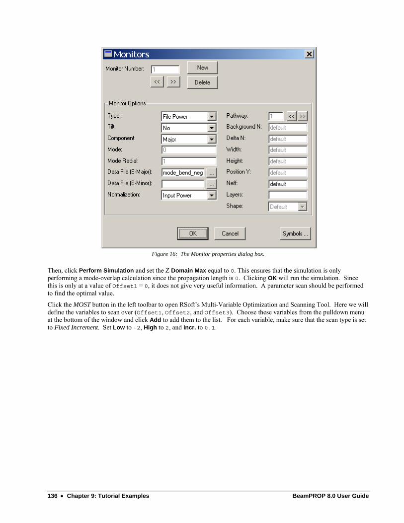
136 • Chapter 9: Tutorial Examples BeamPROP 8.0 User Guide
Figure 16: The Monitor properties dialog box.
Then, click Perform Simulation and set the Z Domain Max equal to 0. This ensures that the simulation is only performing a mode-overlap calculation since the propagation length is 0. Clicking OK will run the simulation. Since this is only at a value of Offset1 = 0, it does not give very useful information. A parameter scan should be performed to find the optimal value.
Click the MOST button in the left toolbar to open RSoft’s Multi-Variable Optimization and Scanning Tool. Here we will define the variables to scan over (Offset1, Offset2, and Offset3). Choose these variables from the pulldown menu at the bottom of the window and click Add to add them to the list. For each variable, make sure that the scan type is set to Fixed Increment. Set Low to -2, High to 2, and Incr. to 0.1.
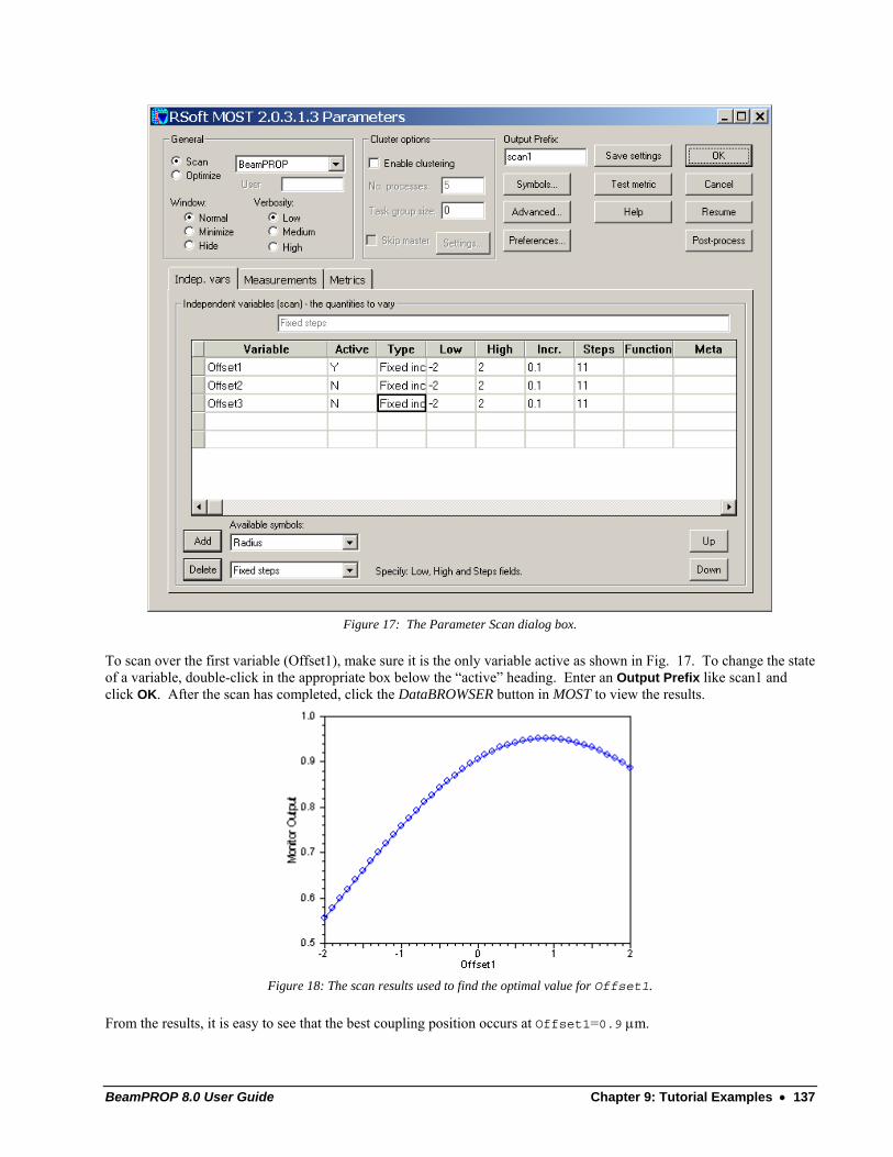
BeamPROP 8.0 User Guide Chapter 9: Tutorial Examples • 137
Figure 17: The Parameter Scan dialog box.
To scan over the first variable (Offset1), make sure it is the only variable active as shown in Fig. 17. To change the state of a variable, double-click in the appropriate box below the “active” heading. Enter an Output Prefix like scan1 and click OK. After the scan has completed, click the DataBROWSER button in MOST to view the results.
Figure 18: The scan results used to find the optimal value for Offset1.
From the results, it is easy to see that the best coupling position occurs at Offset1=0.9 μm.
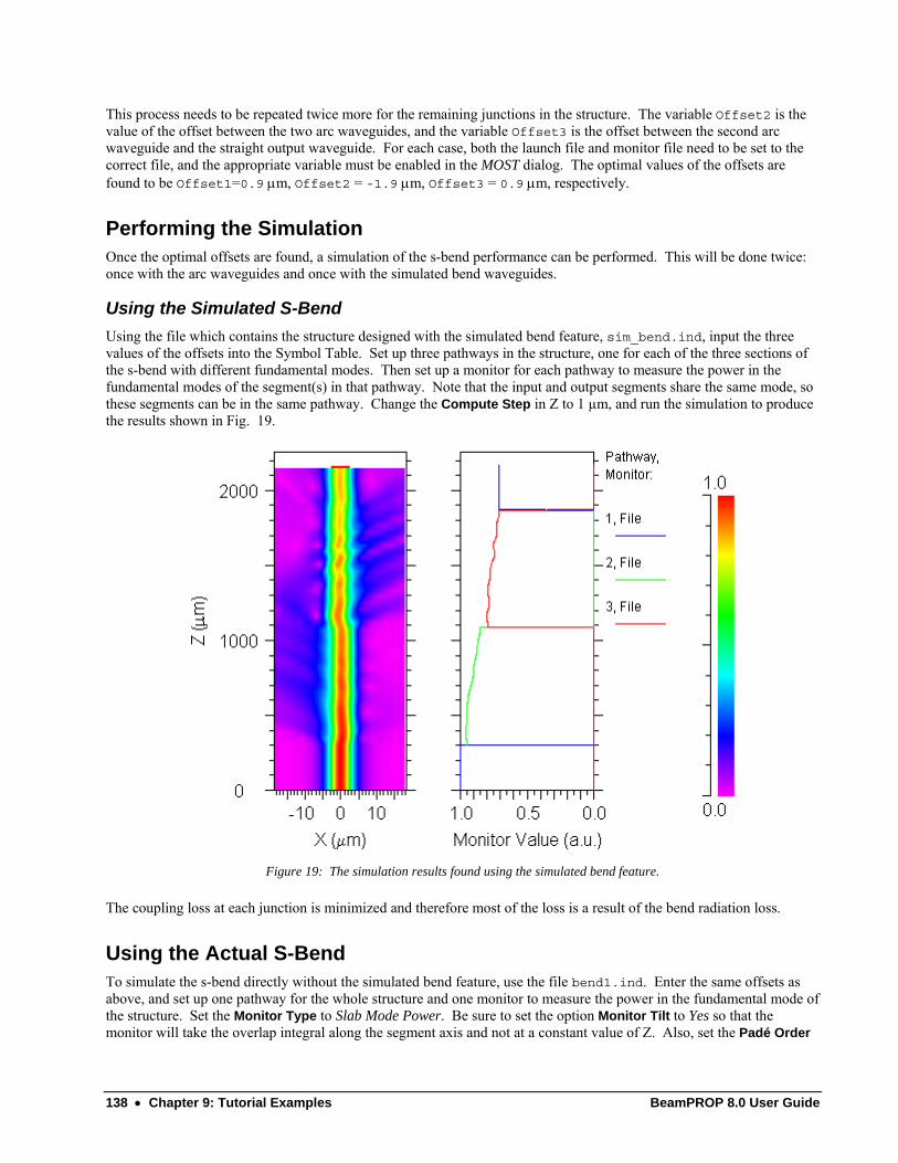
138 • Chapter 9: Tutorial Examples BeamPROP 8.0 User Guide
This process needs to be repeated twice more for the remaining junctions in the structure. The variable Offset2 is the value of the offset between the two arc waveguides, and the variable Offset3 is the offset between the second arc waveguide and the straight output waveguide. For each case, both the launch file and monitor file need to be set to the correct file, and the appropriate variable must be enabled in the MOST dialog. The optimal values of the offsets are found to be Offset1=0.9 μm, Offset2 = -1.9 μm, Offset3 = 0.9 μm, respectively.
Performing the Simulation Once the optimal offsets are found, a simulation of the s-bend performance can be performed. This will be done twice: once with the arc waveguides and once with the simulated bend waveguides.
Using the Simulated S-Bend Using the file which contains the structure designed with the simulated bend feature, sim_bend.ind, input the three values of the offsets into the Symbol Table. Set up three pathways in the structure, one for each of the three sections of the s-bend with different fundamental modes. Then set up a monitor for each pathway to measure the power in the fundamental modes of the segment(s) in that pathway. Note that the input and output segments share the same mode, so these segments can be in the same pathway. Change the Compute Step in Z to 1 µm, and run the simulation to produce the results shown in Fig. 19.
Figure 19: The simulation results found using the simulated bend feature.
The coupling loss at each junction is minimized and therefore most of the loss is a result of the bend radiation loss.
Using the Actual S-Bend To simulate the s-bend directly without the simulated bend feature, use the file bend1.ind. Enter the same offsets as above, and set up one pathway for the whole structure and one monitor to measure the power in the fundamental mode of the structure. Set the Monitor Type to Slab Mode Power. Be sure to set the option Monitor Tilt to Yes so that the monitor will take the overlap integral along the segment axis and not at a constant value of Z. Also, set the Padé Order
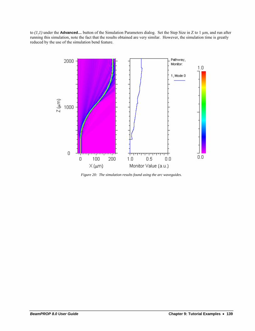
BeamPROP 8.0 User Guide Chapter 9: Tutorial Examples • 139
to (1,1) under the Advanced… button of the Simulation Parameters dialog. Set the Step Size in Z to 1 µm, and run after running this simulation, note the fact that the results obtained are very similar. However, the simulation time is greatly reduced by the use of the simulation bend feature.
Figure 20: The simulation results found using the arc waveguides.

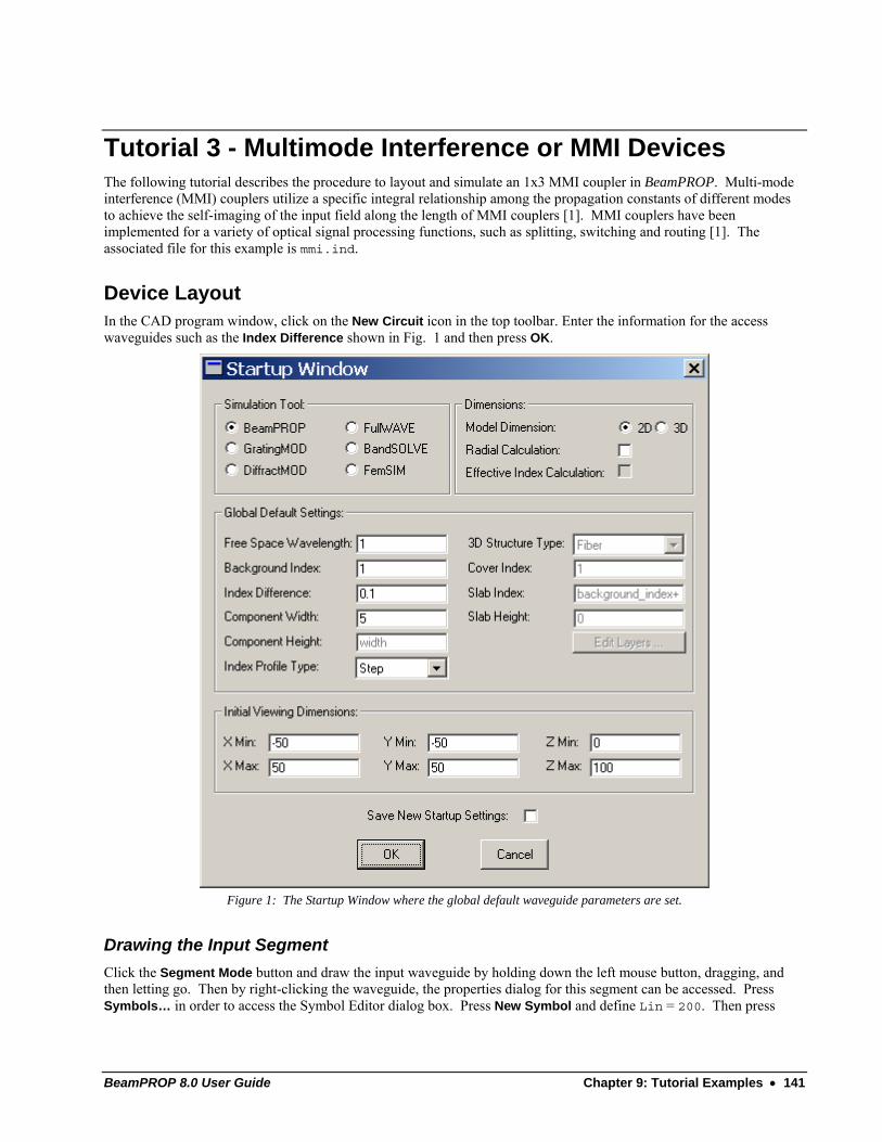
BeamPROP 8.0 User Guide Chapter 9: Tutorial Examples • 141
Tutorial 3 - Multimode Interference or MMI Devices The following tutorial describes the procedure to layout and simulate an 1x3 MMI coupler in BeamPROP. Multi-mode interference (MMI) couplers utilize a specific integral relationship among the propagation constants of different modes to achieve the self-imaging of the input field along the length of MMI couplers [1]. MMI couplers have been implemented for a variety of optical signal processing functions, such as splitting, switching and routing [1]. The associated file for this example is mmi.ind.
Device Layout In the CAD program window, click on the New Circuit icon in the top toolbar. Enter the information for the access waveguides such as the Index Difference shown in Fig. 1 and then press OK.
Figure 1: The Startup Window where the global default waveguide parameters are set.
Drawing the Input Segment Click the Segment Mode button and draw the input waveguide by holding down the left mouse button, dragging, and then letting go. Then by right-clicking the waveguide, the properties dialog for this segment can be accessed. Press Symbols… in order to access the Symbol Editor dialog box. Press New Symbol and define Lin = 200. Then press
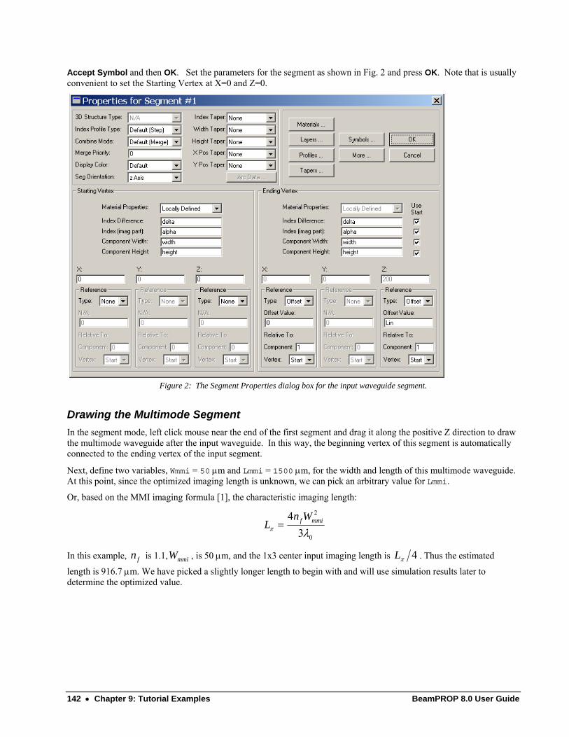
142 • Chapter 9: Tutorial Examples BeamPROP 8.0 User Guide
Accept Symbol and then OK. Set the parameters for the segment as shown in Fig. 2 and press OK. Note that is usually convenient to set the Starting Vertex at X=0 and Z=0.
Figure 2: The Segment Properties dialog box for the input waveguide segment.
Drawing the Multimode Segment In the segment mode, left click mouse near the end of the first segment and drag it along the positive Z direction to draw the multimode waveguide after the input waveguide. In this way, the beginning vertex of this segment is automatically connected to the ending vertex of the input segment.
Next, define two variables, Wmmi = 50 μm and Lmmi = 1500 μm, for the width and length of this multimode waveguide. At this point, since the optimized imaging length is unknown, we can pick an arbitrary value for Lmmi.
Or, based on the MMI imaging formula [1], the characteristic imaging length:
2
0
43f mmin W
Lπ λ=
In this example, fn is 1.1, mmiW , is 50 μm, and the 1x3 center input imaging length is 4πL . Thus the estimated
length is 916.7 μm. We have picked a slightly longer length to begin with and will use simulation results later to determine the optimized value.
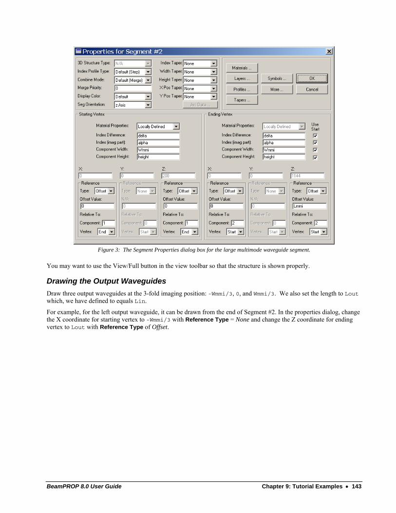
BeamPROP 8.0 User Guide Chapter 9: Tutorial Examples • 143
Figure 3: The Segment Properties dialog box for the large multimode waveguide segment.
You may want to use the View/Full button in the view toolbar so that the structure is shown properly.
Drawing the Output Waveguides Draw three output waveguides at the 3-fold imaging position: -Wmmi/3, 0, and Wmmi/3. We also set the length to Lout which, we have defined to equals Lin.
For example, for the left output waveguide, it can be drawn from the end of Segment #2. In the properties dialog, change the X coordinate for starting vertex to -Wmmi/3 with Reference Type = None and change the Z coordinate for ending vertex to Lout with Reference Type of Offset.
144 • Chapter 9: Tutorial Examples BeamPROP 8.0 User Guide
Figure 4: The Segment Properties dialog box for the left output waveguide.
When the other two output waveguides have been added, the structure will appear in the CAD window as shown in Fig. 5.
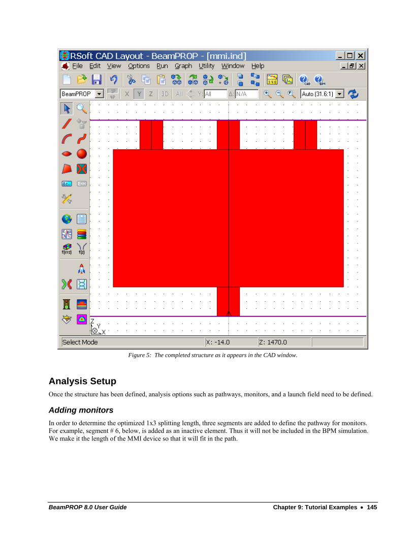
BeamPROP 8.0 User Guide Chapter 9: Tutorial Examples • 145
Figure 5: The completed structure as it appears in the CAD window.
Analysis Setup Once the structure has been defined, analysis options such as pathways, monitors, and a launch field need to be defined.
Adding monitors In order to determine the optimized 1x3 splitting length, three segments are added to define the pathway for monitors. For example, segment # 6, below, is added as an inactive element. Thus it will not be included in the BPM simulation. We make it the length of the MMI device so that it will fit in the path.
146 • Chapter 9: Tutorial Examples BeamPROP 8.0 User Guide
Figure 6: The Segment Properties dialog box for the left inactive segment used only to measure the propagating field. Note that it is
not affect the simulation results in any way.
We make three of these segments. For each one, we change the Starting Vertex, Relative To:, and Offset Value information for both the X and Z coordinates. The structure will now appear as shown in Fig. 7.
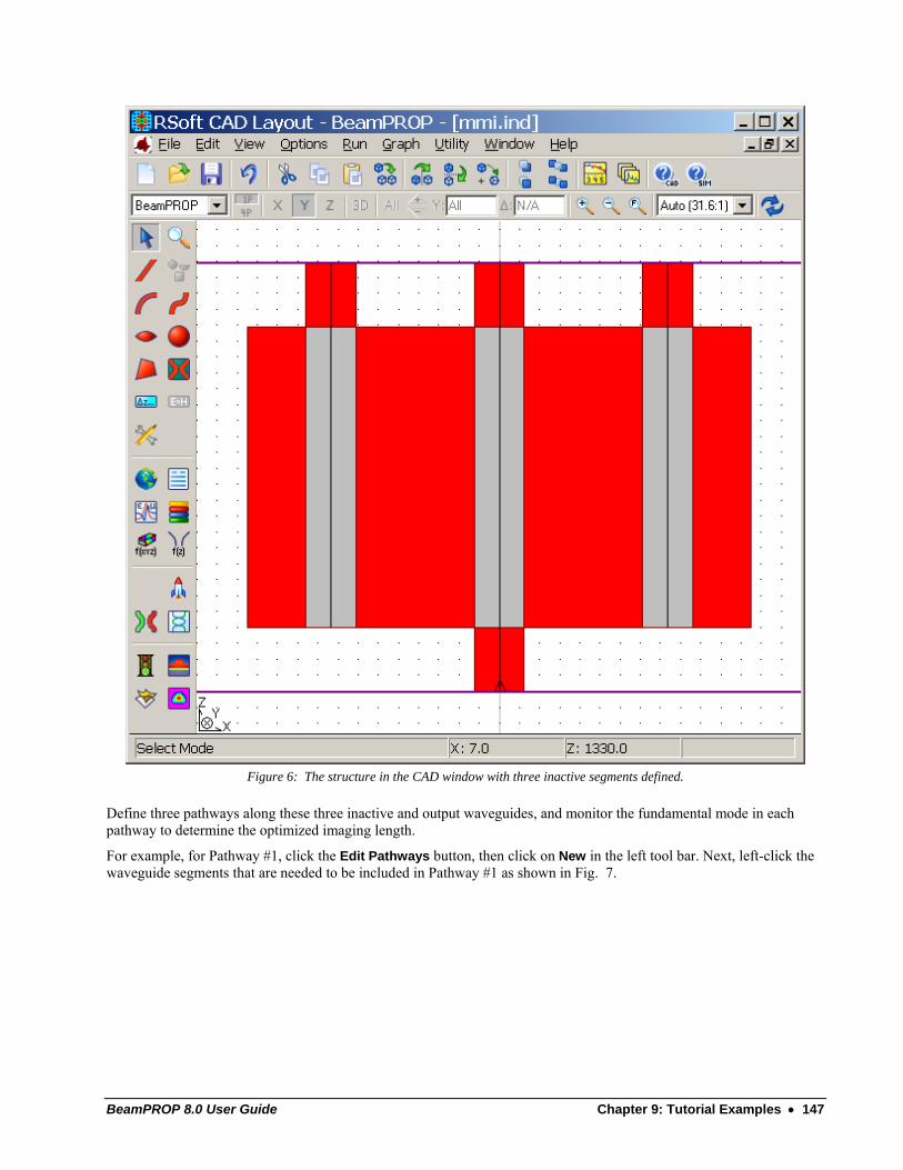
BeamPROP 8.0 User Guide Chapter 9: Tutorial Examples • 147
Figure 6: The structure in the CAD window with three inactive segments defined.
Define three pathways along these three inactive and output waveguides, and monitor the fundamental mode in each pathway to determine the optimized imaging length.
For example, for Pathway #1, click the Edit Pathways button, then click on New in the left tool bar. Next, left-click the waveguide segments that are needed to be included in Pathway #1 as shown in Fig. 7.
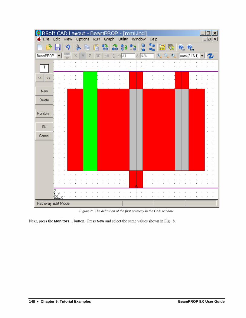
148 • Chapter 9: Tutorial Examples BeamPROP 8.0 User Guide
Figure 7: The definition of the first pathway in the CAD window.
Next, press the Monitors… button. Press New and select the same values shown in Fig. 8.
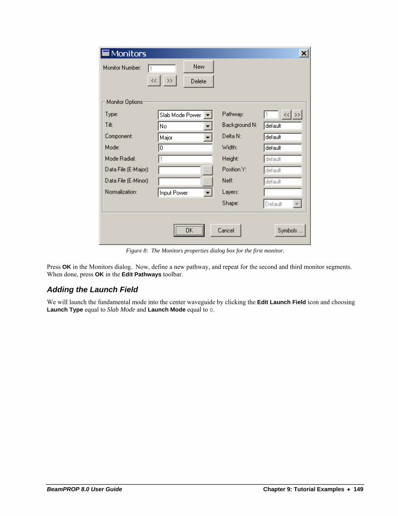
BeamPROP 8.0 User Guide Chapter 9: Tutorial Examples • 149
Figure 8: The Monitors properties dialog box for the first monitor.
Press OK in the Monitors dialog. Now, define a new pathway, and repeat for the second and third monitor segments. When done, press OK in the Edit Pathways toolbar.
Adding the Launch Field We will launch the fundamental mode into the center waveguide by clicking the Edit Launch Field icon and choosing Launch Type equal to Slab Mode and Launch Mode equal to 0.
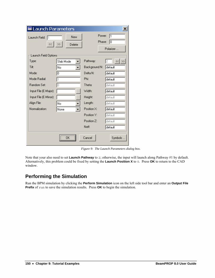
150 • Chapter 9: Tutorial Examples BeamPROP 8.0 User Guide
Figure 9: The Launch Parameters dialog box.
Note that your also need to set Launch Pathway to 2; otherwise, the input will launch along Pathway #1 by default. Alternatively, this problem could be fixed by setting the Launch Position X to 0. Press OK to return to the CAD window.
Performing the Simulation Run the BPM simulation by clicking the Perform Simulation icon on the left side tool bar and enter an Output File Prefix of run to save the simulation results. Press OK to begin the simulation.
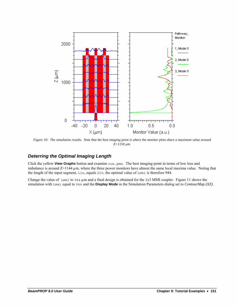
BeamPROP 8.0 User Guide Chapter 9: Tutorial Examples • 151
Figure 10: The simulation results. Note that the best imaging point is where the monitor plots share a maximum value around
Z=1150 μm.
Deterring the Optimal Imaging Length Click the yellow View Graphs button and examine run.pmn. The best imaging point in terms of low loss and imbalance is around Z=1144 μm, where the three power monitors have almost the same local maxima value. Noting that the length of the input segment, Lin, equals 200, the optimal value of Lmmi is therefore 944.
Change the value of Lmmi to 944 μm and a final design is obtained for the 1x3 MMI coupler. Figure 11 shows the simulation with Lmmi equal to 944 and the Display Mode in the Simulation Parameters dialog set to ContourMap (XZ).
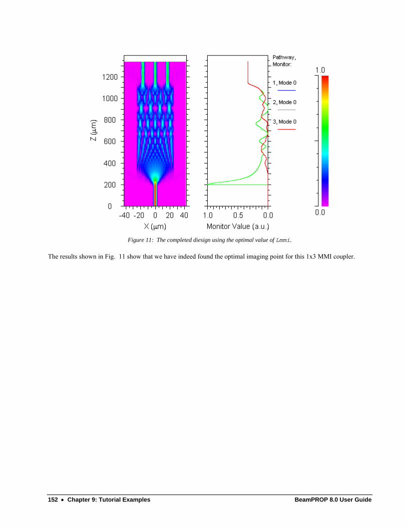
152 • Chapter 9: Tutorial Examples BeamPROP 8.0 User Guide
Figure 11: The completed diesign using the optimal value of Lmmi.
The results shown in Fig. 11 show that we have indeed found the optimal imaging point for this 1x3 MMI coupler.
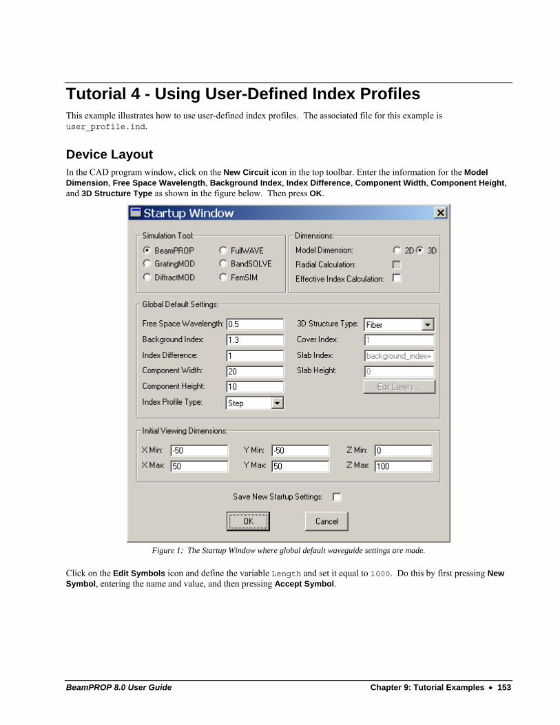
BeamPROP 8.0 User Guide Chapter 9: Tutorial Examples • 153
Tutorial 4 - Using User-Defined Index Profiles This example illustrates how to use user-defined index profiles. The associated file for this example is user_profile.ind.
Device Layout In the CAD program window, click on the New Circuit icon in the top toolbar. Enter the information for the Model Dimension, Free Space Wavelength, Background Index, Index Difference, Component Width, Component Height, and 3D Structure Type as shown in the figure below. Then press OK.
Figure 1: The Startup Window where global default waveguide settings are made.
Click on the Edit Symbols icon and define the variable Length and set it equal to 1000. Do this by first pressing New Symbol, entering the name and value, and then pressing Accept Symbol.
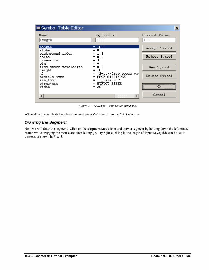
154 • Chapter 9: Tutorial Examples BeamPROP 8.0 User Guide
Figure 2: The Symbol Table Editor diaog box.
When all of the symbols have been entered, press OK to return to the CAD window.
Drawing the Segment Next we will draw the segment. Click on the Segment Mode icon and draw a segment by holding down the left mouse button while dragging the mouse and then letting go. By right-clicking it, the length of input waveguide can be set to Length as shown in Fig. 3.
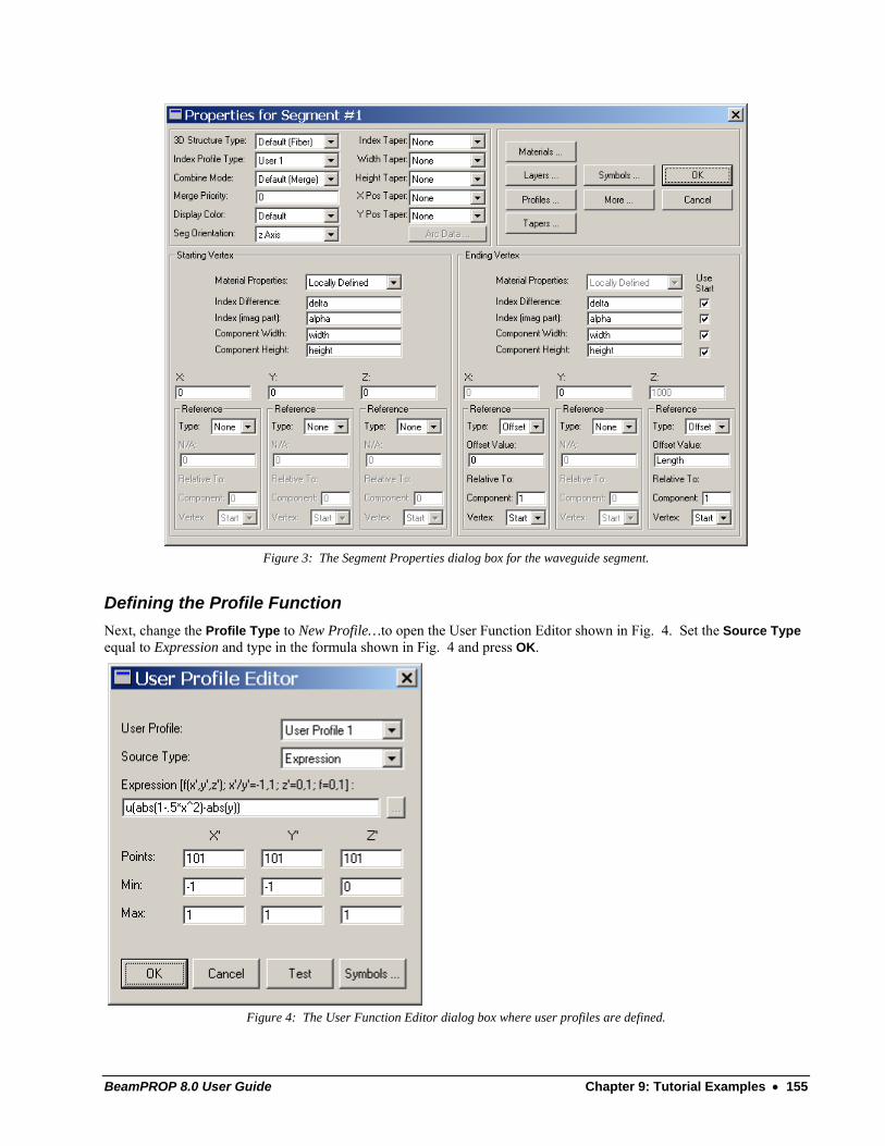
BeamPROP 8.0 User Guide Chapter 9: Tutorial Examples • 155
Figure 3: The Segment Properties dialog box for the waveguide segment.
Defining the Profile Function Next, change the Profile Type to New Profile…to open the User Function Editor shown in Fig. 4. Set the Source Type equal to Expression and type in the formula shown in Fig. 4 and press OK.
Figure 4: The User Function Editor dialog box where user profiles are defined.
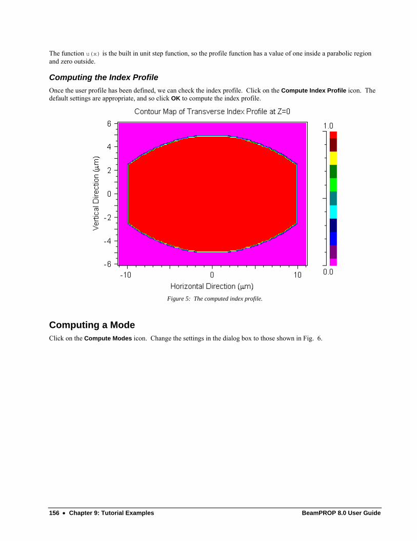
156 • Chapter 9: Tutorial Examples BeamPROP 8.0 User Guide
The function u(x) is the built in unit step function, so the profile function has a value of one inside a parabolic region and zero outside.
Computing the Index Profile Once the user profile has been defined, we can check the index profile. Click on the Compute Index Profile icon. The default settings are appropriate, and so click OK to compute the index profile.
Figure 5: The computed index profile.
Computing a Mode Click on the Compute Modes icon. Change the settings in the dialog box to those shown in Fig. 6.
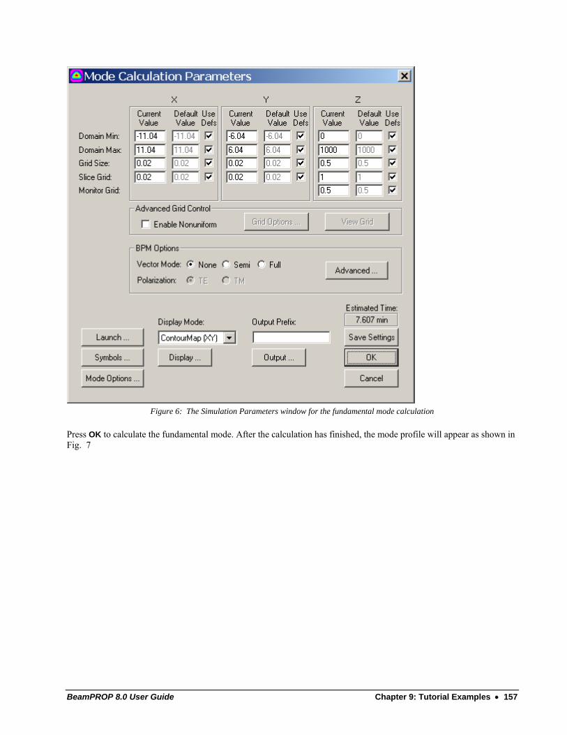
BeamPROP 8.0 User Guide Chapter 9: Tutorial Examples • 157
Figure 6: The Simulation Parameters window for the fundamental mode calculation
Press OK to calculate the fundamental mode. After the calculation has finished, the mode profile will appear as shown in Fig. 7
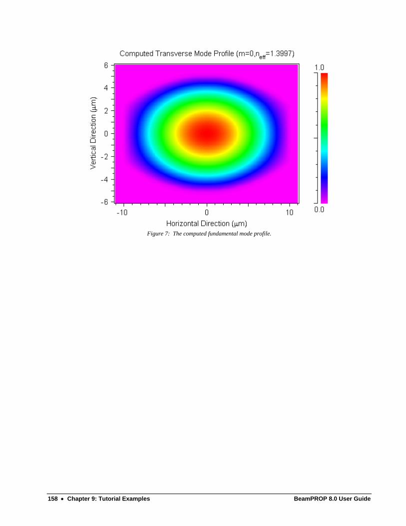
158 • Chapter 9: Tutorial Examples BeamPROP 8.0 User Guide
Figure 7: The computed fundamental mode profile.
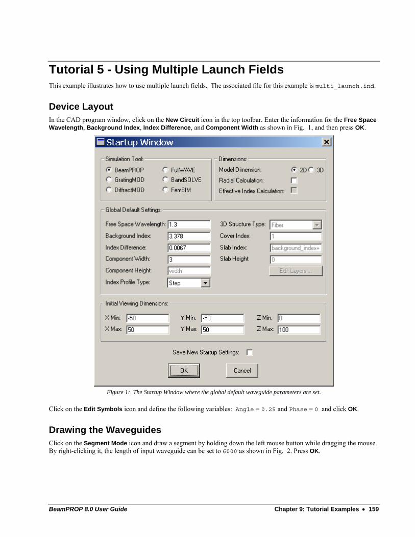
BeamPROP 8.0 User Guide Chapter 9: Tutorial Examples • 159
Tutorial 5 - Using Multiple Launch Fields This example illustrates how to use multiple launch fields. The associated file for this example is multi_launch.ind.
Device Layout In the CAD program window, click on the New Circuit icon in the top toolbar. Enter the information for the Free Space Wavelength, Background Index, Index Difference, and Component Width as shown in Fig. 1, and then press OK.
Figure 1: The Startup Window where the global default waveguide parameters are set.
Click on the Edit Symbols icon and define the following variables: Angle = 0.25 and Phase = 0 and click OK.
Drawing the Waveguides Click on the Segment Mode icon and draw a segment by holding down the left mouse button while dragging the mouse. By right-clicking it, the length of input waveguide can be set to 6000 as shown in Fig. 2. Press OK.
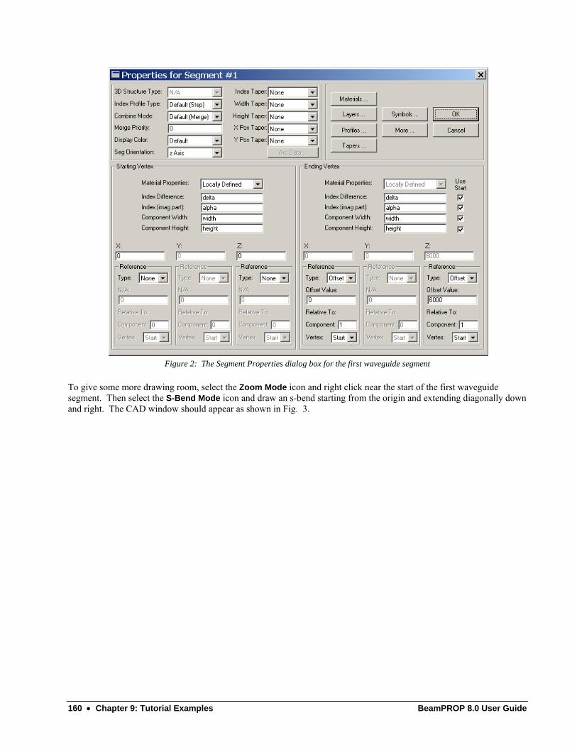
160 • Chapter 9: Tutorial Examples BeamPROP 8.0 User Guide
Figure 2: The Segment Properties dialog box for the first waveguide segment
To give some more drawing room, select the Zoom Mode icon and right click near the start of the first waveguide segment. Then select the S-Bend Mode icon and draw an s-bend starting from the origin and extending diagonally down and right. The CAD window should appear as shown in Fig. 3.
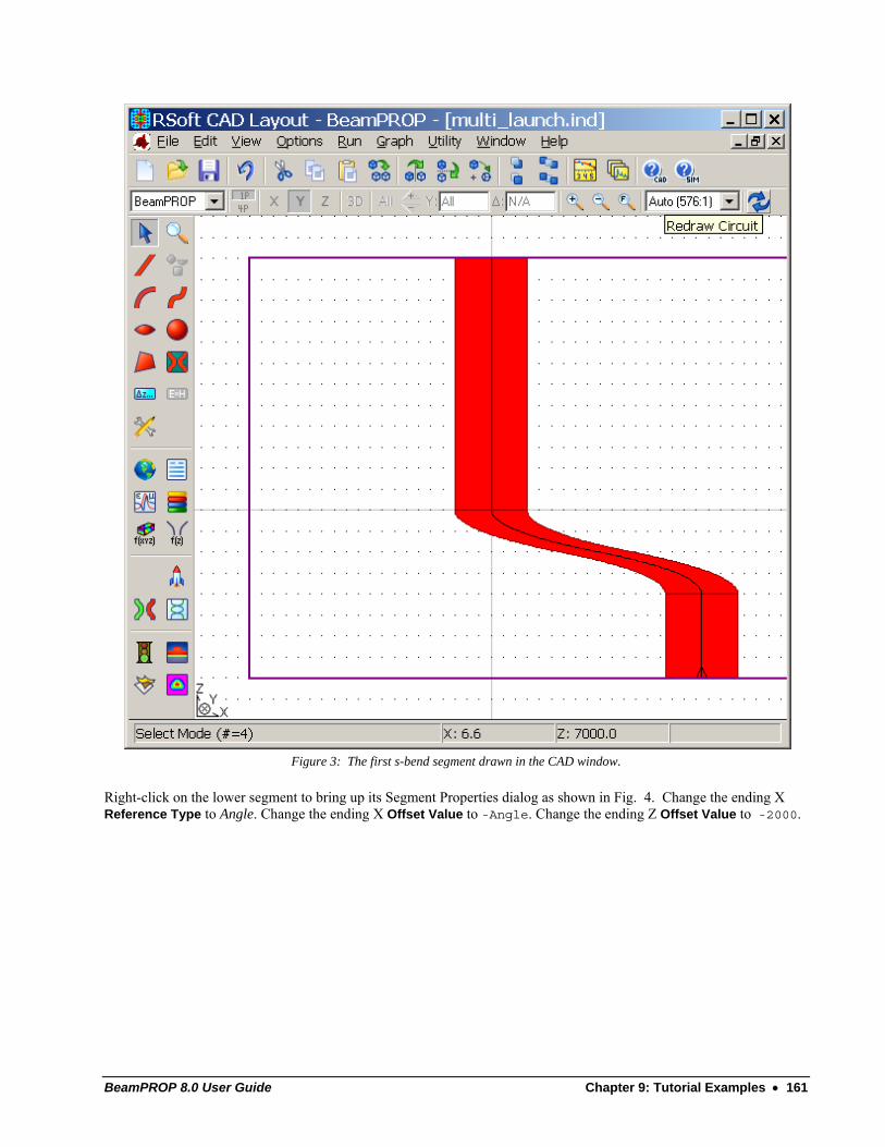
BeamPROP 8.0 User Guide Chapter 9: Tutorial Examples • 161
Figure 3: The first s-bend segment drawn in the CAD window.
Right-click on the lower segment to bring up its Segment Properties dialog as shown in Fig. 4. Change the ending X Reference Type to Angle. Change the ending X Offset Value to -Angle. Change the ending Z Offset Value to -2000.
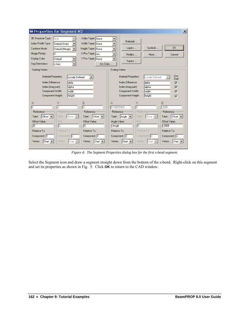
162 • Chapter 9: Tutorial Examples BeamPROP 8.0 User Guide
Figure 4: The Segment Properties dialog box for the first s-bend segment.
Select the Segment icon and draw a segment straight down from the bottom of the s-bend. Right-click on this segment and set its properties as shown in Fig. 5. Click OK to return to the CAD window.
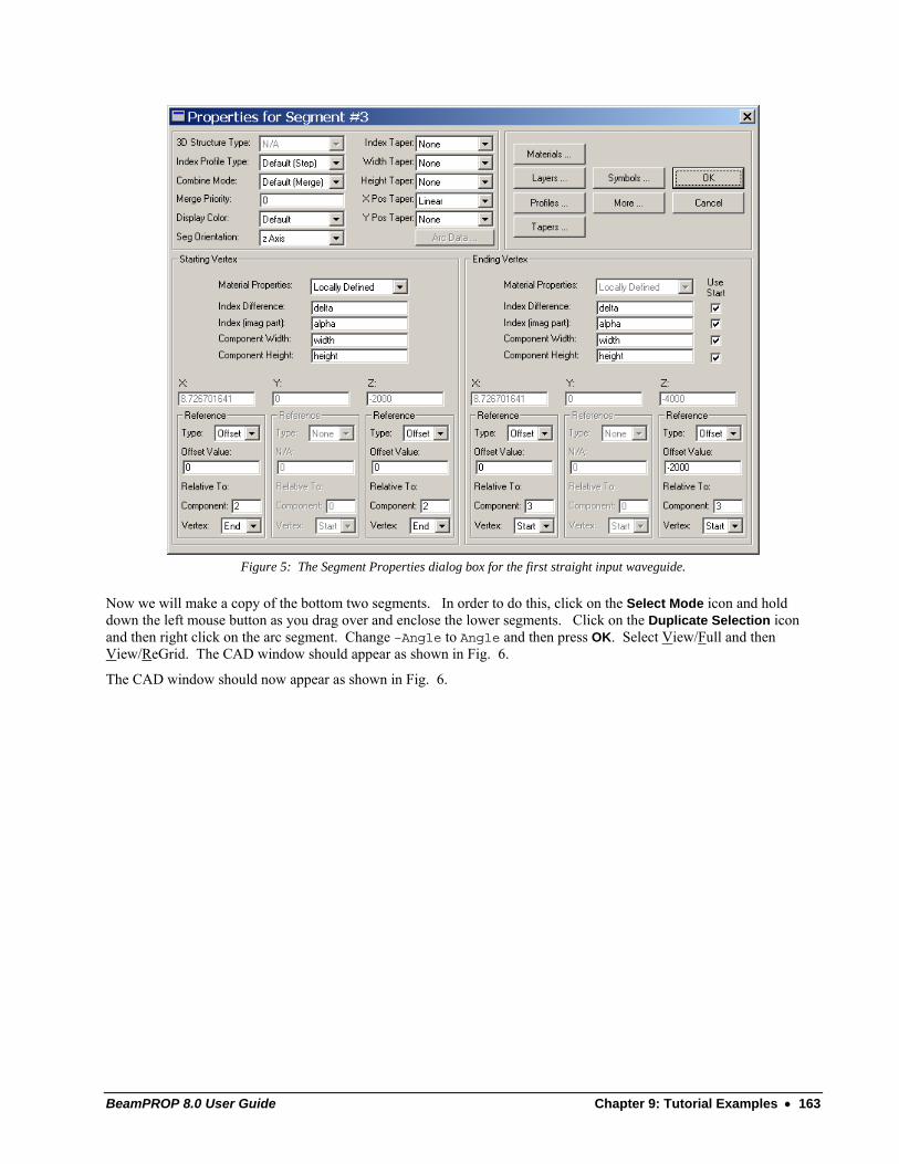
BeamPROP 8.0 User Guide Chapter 9: Tutorial Examples • 163
Figure 5: The Segment Properties dialog box for the first straight input waveguide.
Now we will make a copy of the bottom two segments. In order to do this, click on the Select Mode icon and hold down the left mouse button as you drag over and enclose the lower segments. Click on the Duplicate Selection icon and then right click on the arc segment. Change –Angle to Angle and then press OK. Select View/Full and then View/ReGrid. The CAD window should appear as shown in Fig. 6.
The CAD window should now appear as shown in Fig. 6.
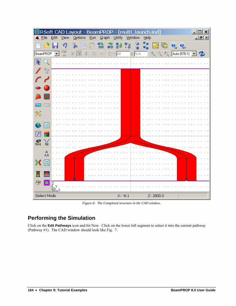
164 • Chapter 9: Tutorial Examples BeamPROP 8.0 User Guide
Figure 6: The Completed structure in the CAD window.
Performing the Simulation Click on the Edit Pathways icon and hit New. Click on the lower left segment to select it into the current pathway (Pathway #1). The CAD window should look like Fig. 7.
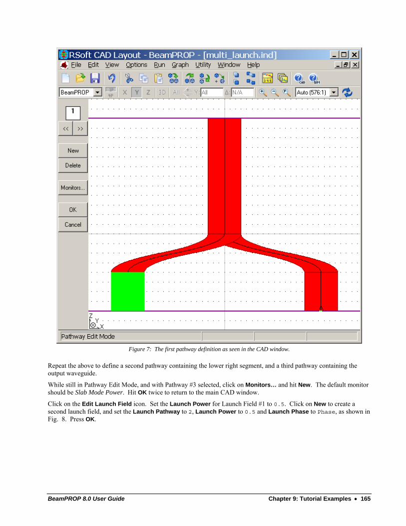
BeamPROP 8.0 User Guide Chapter 9: Tutorial Examples • 165
Figure 7: The first pathway definition as seen in the CAD window.
Repeat the above to define a second pathway containing the lower right segment, and a third pathway containing the output waveguide.
While still in Pathway Edit Mode, and with Pathway #3 selected, click on Monitors… and hit New. The default monitor should be Slab Mode Power. Hit OK twice to return to the main CAD window.
Click on the Edit Launch Field icon. Set the Launch Power for Launch Field #1 to 0.5. Click on New to create a second launch field, and set the Launch Pathway to 2, Launch Power to 0.5 and Launch Phase to Phase, as shown in Fig. 8. Press OK.
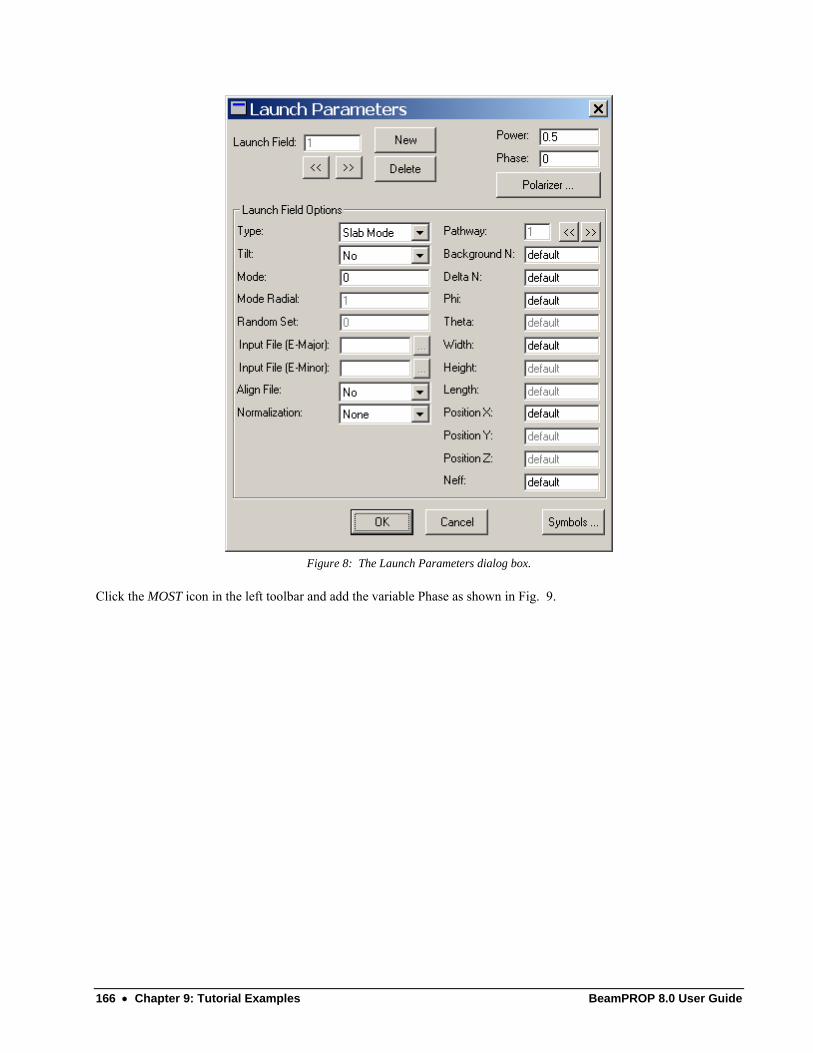
166 • Chapter 9: Tutorial Examples BeamPROP 8.0 User Guide
Figure 8: The Launch Parameters dialog box.
Click the MOST icon in the left toolbar and add the variable Phase as shown in Fig. 9.
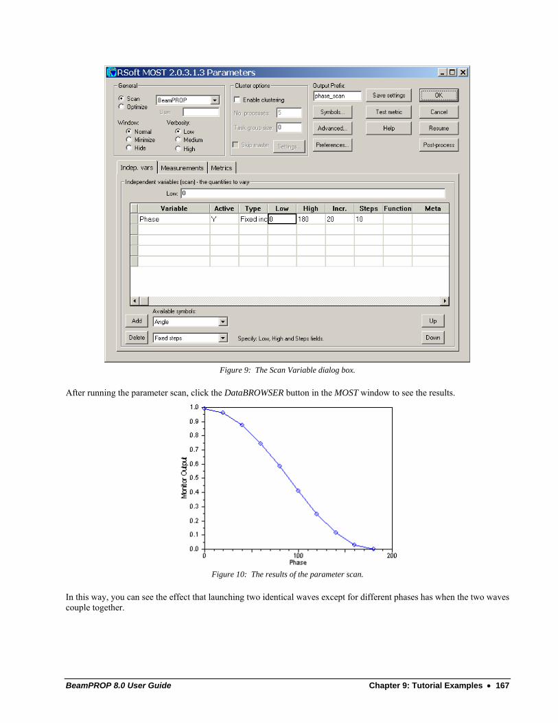
BeamPROP 8.0 User Guide Chapter 9: Tutorial Examples • 167
Figure 9: The Scan Variable dialog box.
After running the parameter scan, click the DataBROWSER button in the MOST window to see the results.
Figure 10: The results of the parameter scan.
In this way, you can see the effect that launching two identical waves except for different phases has when the two waves couple together.

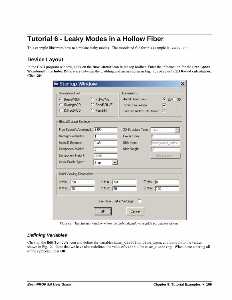
BeamPROP 8.0 User Guide Chapter 9: Tutorial Examples • 169
Tutorial 6 - Leaky Modes in a Hollow Fiber This example illustrates how to simulate leaky modes. The associated file for this example is leaky.ind.
Device Layout In the CAD program window, click on the New Circuit icon in the top toolbar. Enter the information for the Free Space Wavelength, the Index Difference between the cladding and air as shown in Fig. 1, and select a 2D Radial calculation. Click OK.
Figure 1: The Startup Window where the global default waveguide parameters are set.
Defining Variables Click on the Edit Symbols icon and define the variables Diam_Cladding, Diam_Core, and Length to the values shown in Fig. 2. Note that we have also redefined the value of width to be Diam_Cladding. When done entering all of the symbols, press OK.
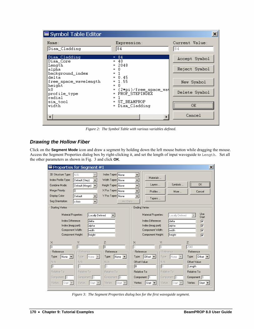
170 • Chapter 9: Tutorial Examples BeamPROP 8.0 User Guide
Figure 2: The Symbol Table with various variables defined.
Drawing the Hollow Fiber Click on the Segment Mode icon and draw a segment by holding down the left mouse button while dragging the mouse. Access the Segment Properties dialog box by right-clicking it, and set the length of input waveguide to Length. Set all the other parameters as shown in Fig. 3 and click OK.
Figure 3: The Segment Properties dialog box for the first waveguide segment.
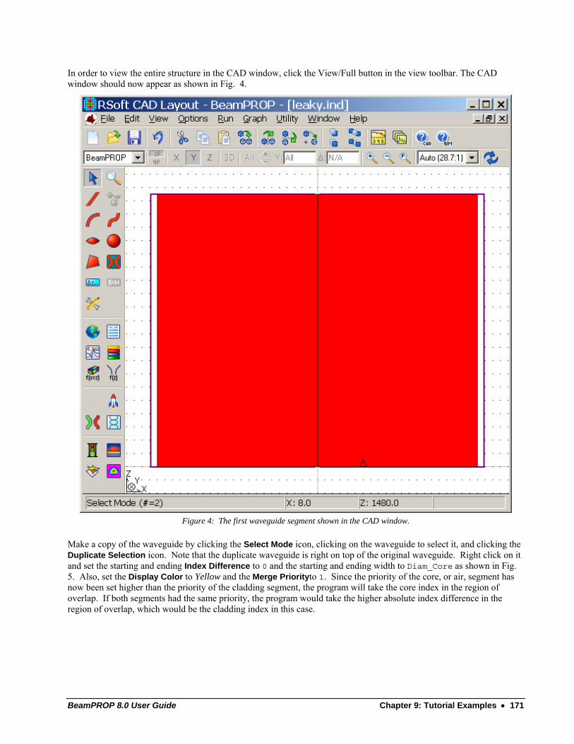
BeamPROP 8.0 User Guide Chapter 9: Tutorial Examples • 171
In order to view the entire structure in the CAD window, click the View/Full button in the view toolbar. The CAD window should now appear as shown in Fig. 4.
Figure 4: The first waveguide segment shown in the CAD window.
Make a copy of the waveguide by clicking the Select Mode icon, clicking on the waveguide to select it, and clicking the Duplicate Selection icon. Note that the duplicate waveguide is right on top of the original waveguide. Right click on it and set the starting and ending Index Difference to 0 and the starting and ending width to Diam_Core as shown in Fig. 5. Also, set the Display Color to Yellow and the Merge Priorityto 1. Since the priority of the core, or air, segment has now been set higher than the priority of the cladding segment, the program will take the core index in the region of overlap. If both segments had the same priority, the program would take the higher absolute index difference in the region of overlap, which would be the cladding index in this case.
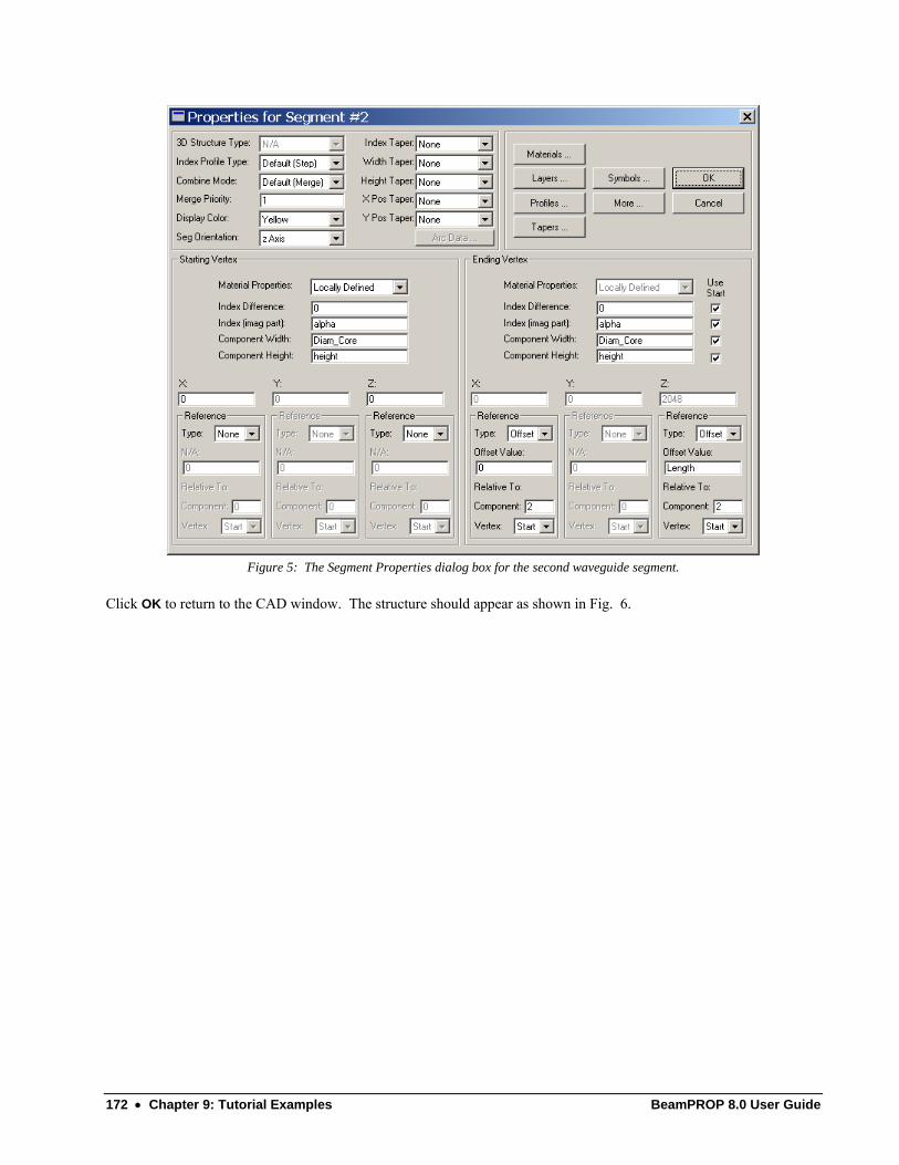
172 • Chapter 9: Tutorial Examples BeamPROP 8.0 User Guide
Figure 5: The Segment Properties dialog box for the second waveguide segment.
Click OK to return to the CAD window. The structure should appear as shown in Fig. 6.
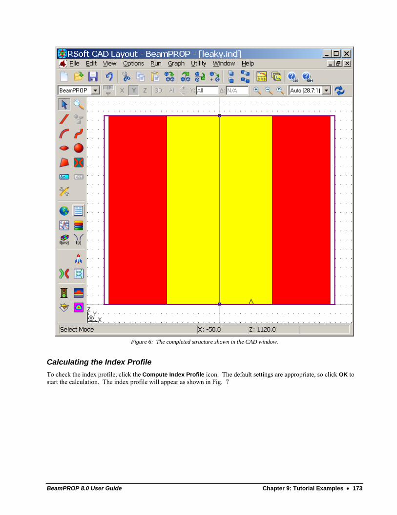
BeamPROP 8.0 User Guide Chapter 9: Tutorial Examples • 173
Figure 6: The completed structure shown in the CAD window.
Calculating the Index Profile To check the index profile, click the Compute Index Profile icon. The default settings are appropriate, so click OK to start the calculation. The index profile will appear as shown in Fig. 7
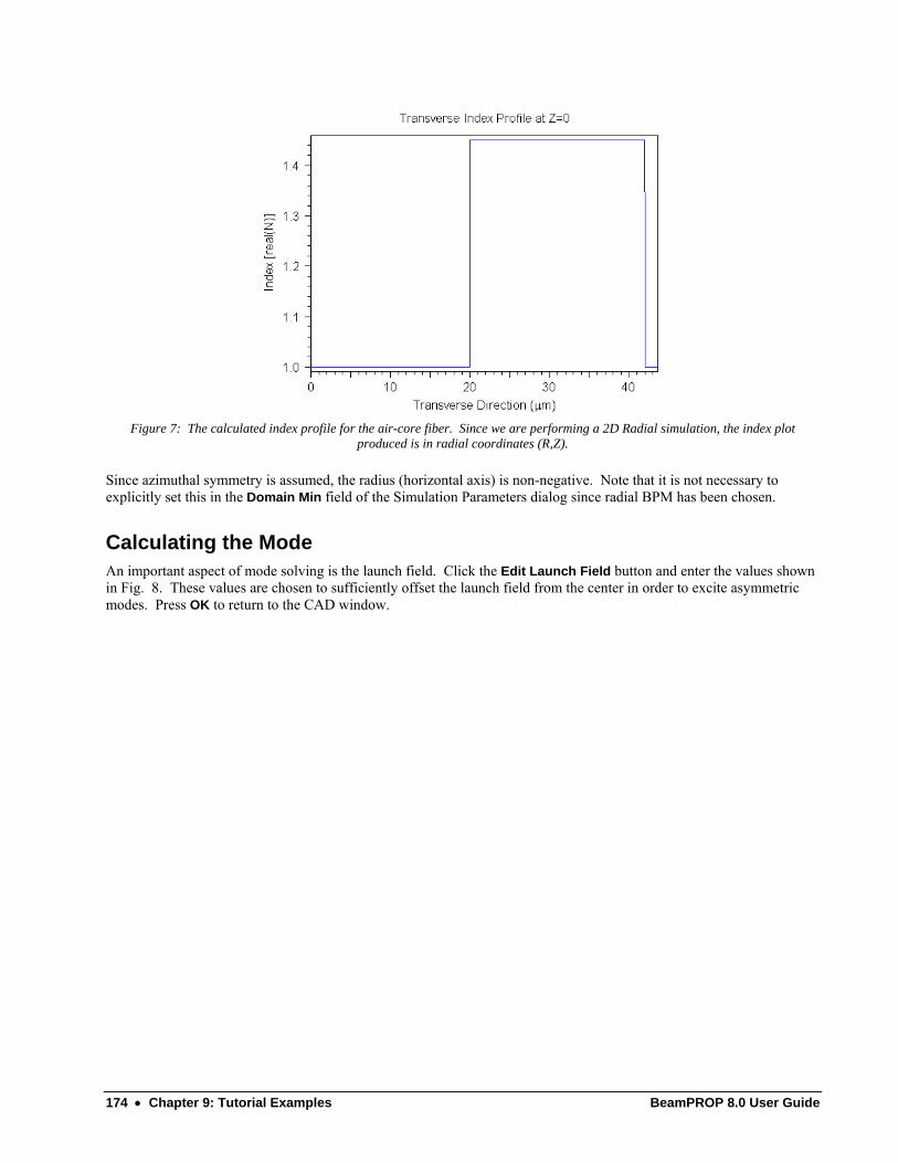
174 • Chapter 9: Tutorial Examples BeamPROP 8.0 User Guide
Figure 7: The calculated index profile for the air-core fiber. Since we are performing a 2D Radial simulation, the index plot
produced is in radial coordinates (R,Z).
Since azimuthal symmetry is assumed, the radius (horizontal axis) is non-negative. Note that it is not necessary to explicitly set this in the Domain Min field of the Simulation Parameters dialog since radial BPM has been chosen.
Calculating the Mode An important aspect of mode solving is the launch field. Click the Edit Launch Field button and enter the values shown in Fig. 8. These values are chosen to sufficiently offset the launch field from the center in order to excite asymmetric modes. Press OK to return to the CAD window.
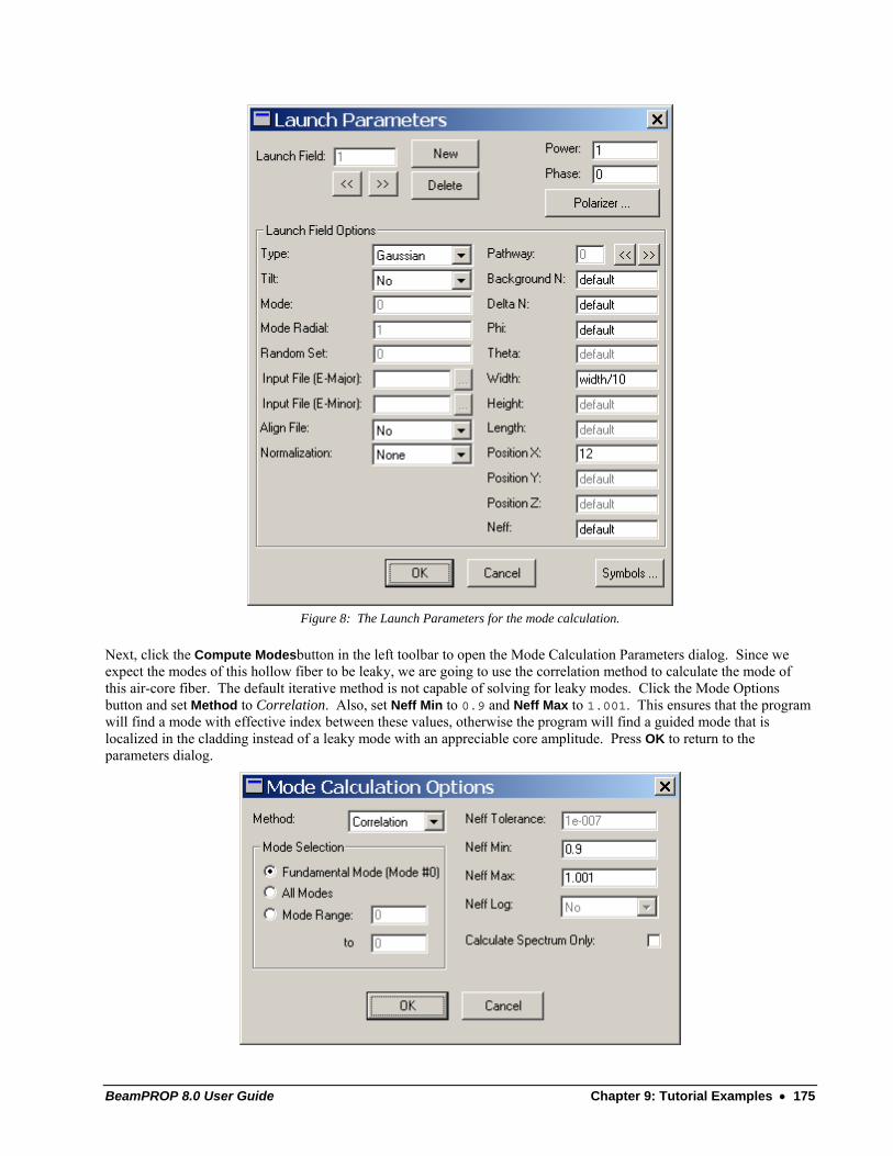
BeamPROP 8.0 User Guide Chapter 9: Tutorial Examples • 175
Figure 8: The Launch Parameters for the mode calculation.
Next, click the Compute Modesbutton in the left toolbar to open the Mode Calculation Parameters dialog. Since we expect the modes of this hollow fiber to be leaky, we are going to use the correlation method to calculate the mode of this air-core fiber. The default iterative method is not capable of solving for leaky modes. Click the Mode Options button and set Method to Correlation. Also, set Neff Min to 0.9 and Neff Max to 1.001. This ensures that the program will find a mode with effective index between these values, otherwise the program will find a guided mode that is localized in the cladding instead of a leaky mode with an appreciable core amplitude. Press OK to return to the parameters dialog.
176 • Chapter 9: Tutorial Examples BeamPROP 8.0 User Guide
Figure 9: The Mode Calculation Options dialog box.
We are use the default grid sizes which are relatively large so as to decrease the simulation time.
Figure 10: The Simulation Parameters for the mode computation.
Next, click the Advanced… button to set the reference k value as well as the boundary condition. Set the Boundary Condition to Simple TBC and change Reference k to k External. This latter step is necessary because the program
would normally attempt to choose a reference wavenumber corresponding to the fundamental guided mode. However, in this case we are interested in leaky modes which have a reference wavenumber near the background index, which is air
in this example.
BeamPROP 8.0 User Guide Chapter 9: Tutorial Examples • 177
Figure 11: The Advanced Parameters dialog box.
Press OK twice to start the mode calculation. The calculated mode will be displayed as shown in Fig. 12.
Figure 12: The computed mode with large grid sizes. Note that the imaginay part of the mode’s effeicve index is displayed on the top
of this window.
178 • Chapter 9: Tutorial Examples BeamPROP 8.0 User Guide
Refining the Calculation If we now set the compute step sizes back to the default, we will see cladding oscillations and get a more accurate value of the effective index, however the simulation will take slightly longer. Click on the Compute Fundamental Mode icon, set the grid sizes to the defaults, and press OK. The computed mode will appear as shown in Fig. 13.
Figure 13: The computed mode found with smaller grid sizes. Again, note the imaginary part of the mode’s effective index at the top
of this window.
BeamPROP 8.0 User Guide Chapter 9: Tutorial Examples • 179
Tutorial 7 - Using Wide-Angle BPM The basic BPM algorithm is fundamentally for paraxial propagation. However, many waveguide structures require propagation at angles larger than ~10-15 degrees from the optical axis, which is the z-axis in the CAD. This is typically the limits of what can be considered paraxial. As discussed in Section 2.B.4, BeamPROP has enhancements to the standard algorithm for wide-angle propagation. This technique uses Padé Approximants to relax, to varying degrees, the paraxial approximation inherent in the BPM, without sacrificing its numerical advantages.
This tutorial describes a step by step procedure on how to adjust the parameters necessary to account for wide-angle propagation. The example circuit will be a straight waveguide that extends at an angle from the optical axis. Various simulations will be conducted to demonstrate the effects of wide-angle propagation and how these effects are ameliorated via use of higher Padé orders. Additionally, appropriate Pathways, Monitors, and launch fields will be chosen. The associated file for this example is wideangle.ind.
Note that this example will be conducted in 2D, though most of the issues also apply to 3D simulations. In 3D, there are fewer Padé orders available.
Additionally, this tutorial illustrates the concept of a convergence study. Please see the closing remarks at the end of the tutorial for more details.
Device Layout Begin by launching the CAD program and click the New Circuit icon and click OK to accept the default parameters, which will suffice for this example.
Before drawing any waveguides, it will be convenient to define several variables in the Symbol Table. To do this, click the Edit Symbols icon, which will bring up the Symbol Table. Define a variable named Angle and set its value to 20. This variable will represent the number of degrees, from the z-axis, along which the waveguide will lie.
Figure 1: The Symbol Table Editor.
Use the left mouse button to draw a waveguide starting from the origin as shown in Fig. 2.
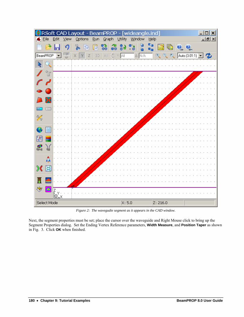
180 • Chapter 9: Tutorial Examples BeamPROP 8.0 User Guide
Figure 2: The wavegudie segment as it appears in the CAD window.
Next, the segment properties must be set; place the cursor over the waveguide and Right Mouse click to bring up the Segment Properties dialog. Set the Ending Vertex Reference parameters, Width Measure, and Position Taper as shown in Fig. 3. Click OK when finished.
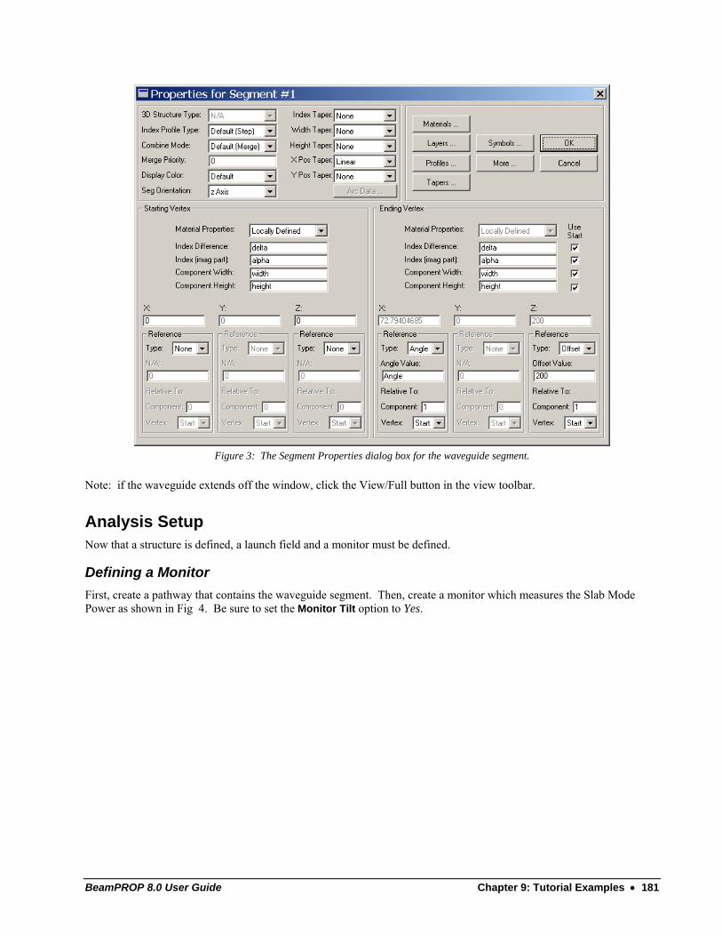
BeamPROP 8.0 User Guide Chapter 9: Tutorial Examples • 181
Figure 3: The Segment Properties dialog box for the waveguide segment.
Note: if the waveguide extends off the window, click the View/Full button in the view toolbar.
Analysis Setup Now that a structure is defined, a launch field and a monitor must be defined.
Defining a Monitor First, create a pathway that contains the waveguide segment. Then, create a monitor which measures the Slab Mode Power as shown in Fig 4. Be sure to set the Monitor Tilt option to Yes.
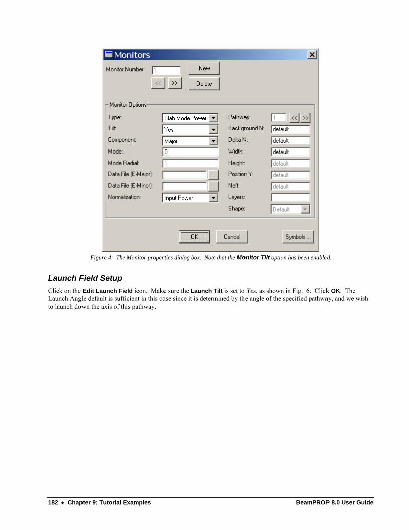
182 • Chapter 9: Tutorial Examples BeamPROP 8.0 User Guide
Figure 4: The Monitor properties dialog box. Note that the Monitor Tilt option has been enabled.
Launch Field Setup Click on the Edit Launch Field icon. Make sure the Launch Tilt is set to Yes, as shown in Fig. 6. Click OK. The Launch Angle default is sufficient in this case since it is determined by the angle of the specified pathway, and we wish to launch down the axis of this pathway.
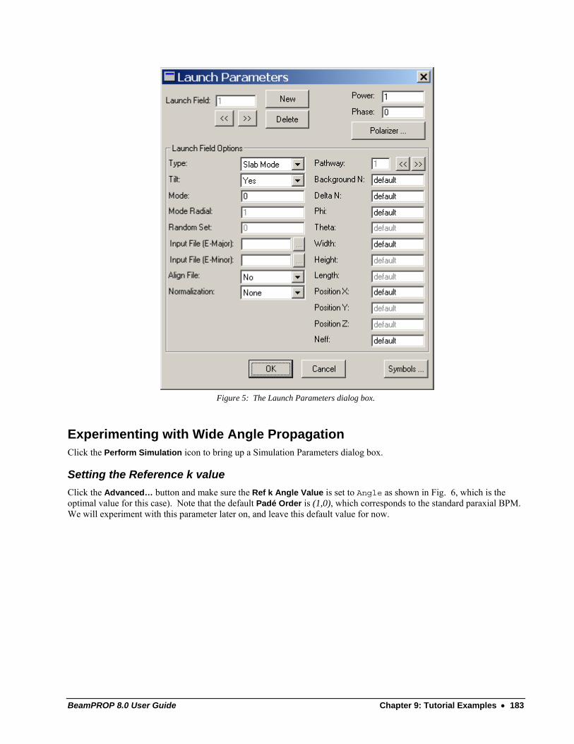
BeamPROP 8.0 User Guide Chapter 9: Tutorial Examples • 183
Figure 5: The Launch Parameters dialog box.
Experimenting with Wide Angle Propagation Click the Perform Simulation icon to bring up a Simulation Parameters dialog box.
Setting the Reference k value Click the Advanced… button and make sure the Ref k Angle Value is set to Angle as shown in Fig. 6, which is the optimal value for this case). Note that the default Padé Order is (1,0), which corresponds to the standard paraxial BPM. We will experiment with this parameter later on, and leave this default value for now.
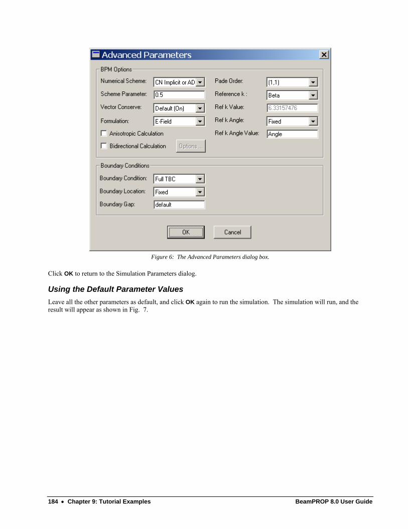
184 • Chapter 9: Tutorial Examples BeamPROP 8.0 User Guide
Figure 6: The Advanced Parameters dialog box.
Click OK to return to the Simulation Parameters dialog.
Using the Default Parameter Values Leave all the other parameters as default, and click OK again to run the simulation. The simulation will run, and the result will appear as shown in Fig. 7.
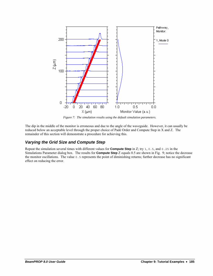
BeamPROP 8.0 User Guide Chapter 9: Tutorial Examples • 185
Figure 7: The simulation results using the default simulation parameters.
The dip in the middle of the monitor is erroneous and due to the angle of the waveguide. However, it can usually be reduced below an acceptable level through the proper choice of Padé Order and Compute Step in X and Z. The remainder of this section will demonstrate a procedure for achieving this.
Varying the Grid Size and Compute Step Repeat the simulation several times with different values for Compute Step in Z; try 1, 0.5, and 0.25 in the Simulations Parameter dialog box. The results for Compute Step Z equals 0.5 are shown in Fig. 9; notice the decrease the monitor oscillations. The value 0.5 represents the point of diminishing returns; further decrease has no significant effect on reducing the error.
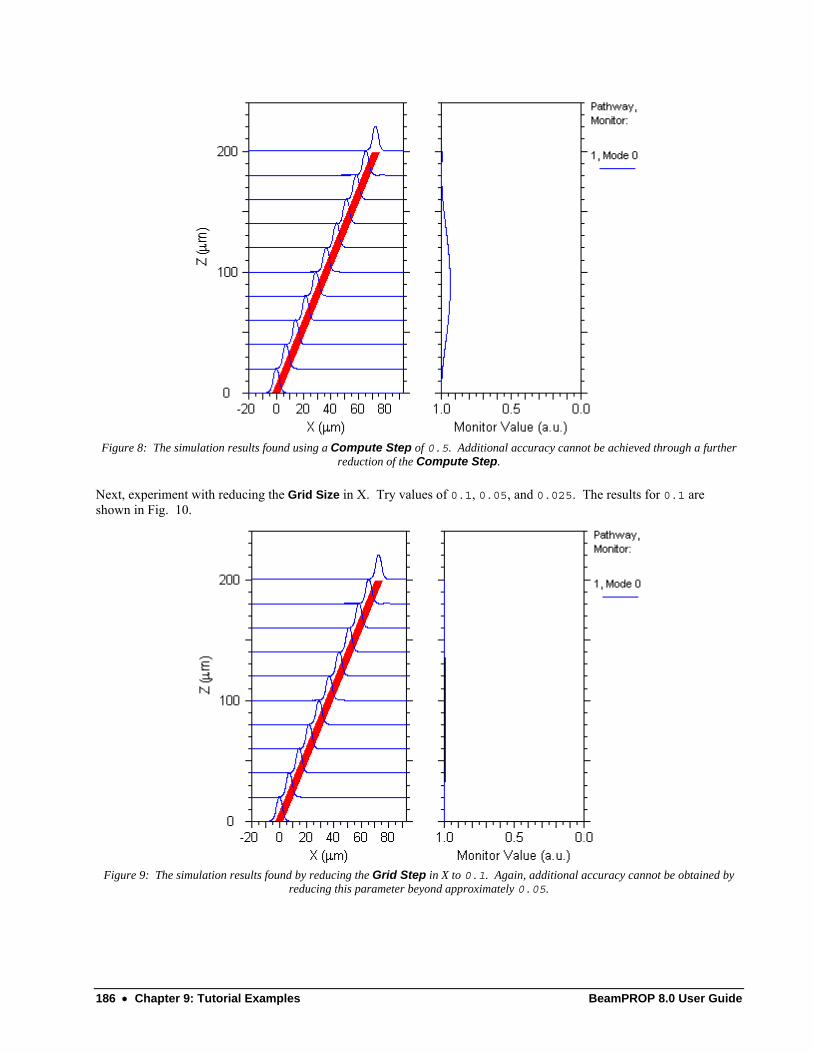
186 • Chapter 9: Tutorial Examples BeamPROP 8.0 User Guide
Figure 8: The simulation results found using a Compute Step of 0.5. Additional accuracy cannot be achieved through a further
reduction of the Compute Step.
Next, experiment with reducing the Grid Size in X. Try values of 0.1, 0.05, and 0.025. The results for 0.1 are shown in Fig. 10.
Figure 9: The simulation results found by reducing the Grid Step in X to 0.1. Again, additional accuracy cannot be obtained by
reducing this parameter beyond approximately 0.05.
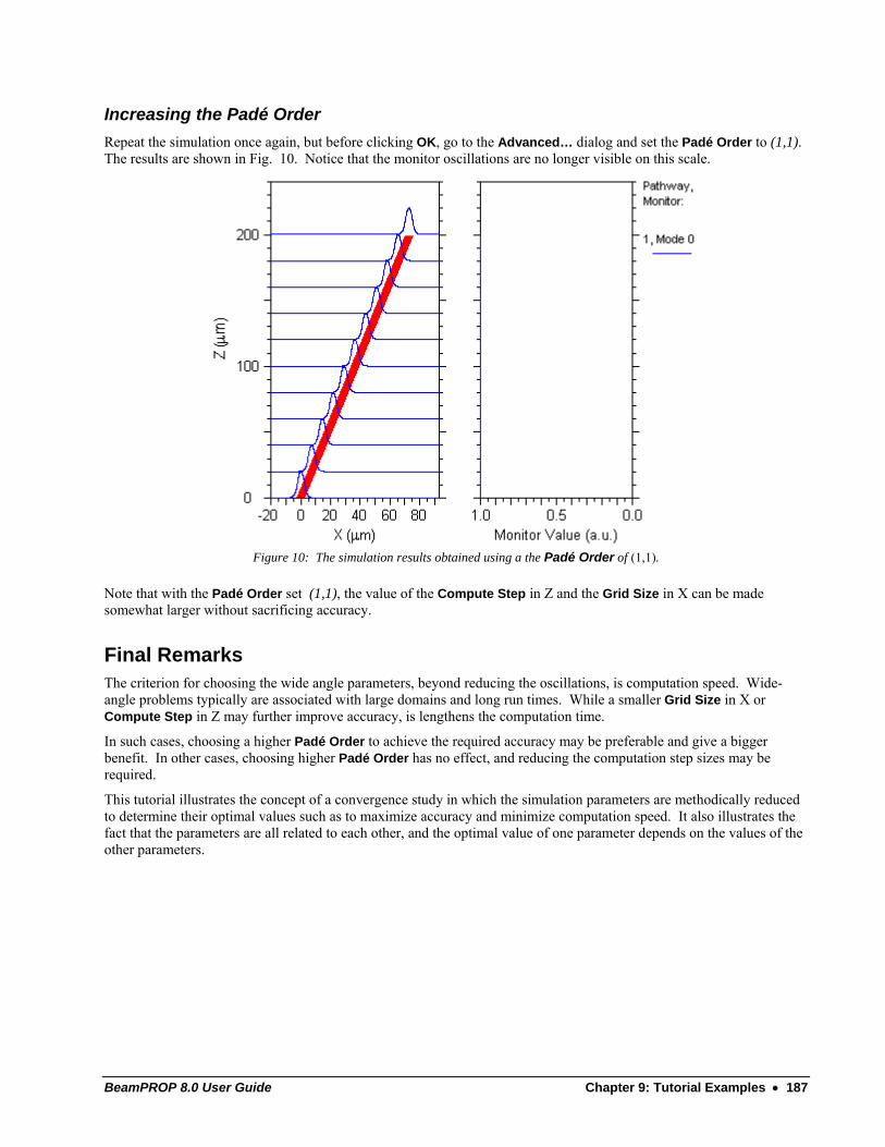
BeamPROP 8.0 User Guide Chapter 9: Tutorial Examples • 187
Increasing the Padé Order Repeat the simulation once again, but before clicking OK, go to the Advanced… dialog and set the Padé Order to (1,1). The results are shown in Fig. 10. Notice that the monitor oscillations are no longer visible on this scale.
Figure 10: The simulation results obtained using a the Padé Order of (1,1).
Note that with the Padé Order set (1,1), the value of the Compute Step in Z and the Grid Size in X can be made somewhat larger without sacrificing accuracy.
Final Remarks The criterion for choosing the wide angle parameters, beyond reducing the oscillations, is computation speed. Wide-angle problems typically are associated with large domains and long run times. While a smaller Grid Size in X or Compute Step in Z may further improve accuracy, is lengthens the computation time.
In such cases, choosing a higher Padé Order to achieve the required accuracy may be preferable and give a bigger benefit. In other cases, choosing higher Padé Order has no effect, and reducing the computation step sizes may be required.
This tutorial illustrates the concept of a convergence study in which the simulation parameters are methodically reduced to determine their optimal values such as to maximize accuracy and minimize computation speed. It also illustrates the fact that the parameters are all related to each other, and the optimal value of one parameter depends on the values of the other parameters.


BeamPROP 8.0 User Guide Chapter 9: Tutorial Examples • 189
Tutorial 8 - Using Bidirectional BPM for Modeling Gratings Many waveguide structures, such as Bragg Gratings, contain perturbations along the direction of propagation (z direction).The standard unidirectional BPM algorithm will fail to account for the coupling caused by these perturbations between the forward and backward propagating fields. To accommodate these situations, several algorithms for Bidirectional BPM are implemented in BeamPROP. These techniques take into account wave propagation in both directions and provide a means for determining the steady state field. This feature is currently only available for 2D problems, and it works best for, but is not restricted to, situations in which the index contrast (perturbation) is small and the paraxiality condition is satisfied (both forward and backward waves propagate along, or nearly along the z axis). The Bidirectional BPM feature is documented in Section 7.C.
This tutorial describes a step by step procedure on how to create and simulate a grating using the bidirectional feature that will entail a scan over the free space wavelength so as to determine the grating spectrum. The tutorial will also discuss how to use such features as “User Tapers,” establishing Pathways and Monitors, and setting the appropriate launch and simulation parameters. The associated file for this example is grating.ind.
Device Layout Begin by launching the CAD program from either the Window’s Start Menu program group or from the Desktop icon.
Creating the Circuit Click the New Circuit icon and adjust the following values for the Free Space Wavelength, Background Index, Index Difference, and Component Width shown in the Startup Window dialog box as shown in Figure 1. Click OK when finished.
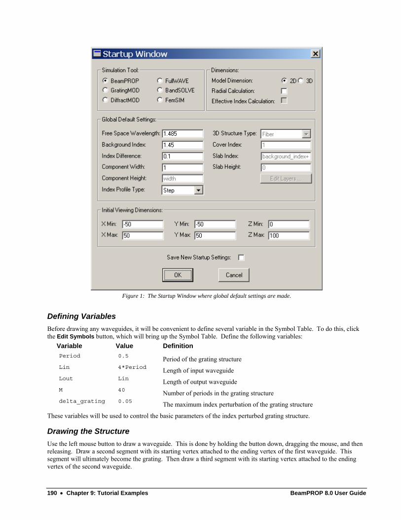
190 • Chapter 9: Tutorial Examples BeamPROP 8.0 User Guide
Figure 1: The Startup Window where global default settings are made.
Defining Variables Before drawing any waveguides, it will be convenient to define several variable in the Symbol Table. To do this, click the Edit Symbols button, which will bring up the Symbol Table. Define the following variables: Variable Value Definition Period 0.5 Period of the grating structure Lin 4*Period Length of input waveguide Lout Lin Length of output waveguide M 40 Number of periods in the grating structure delta_grating 0.05 The maximum index perturbation of the grating structure
These variables will be used to control the basic parameters of the index perturbed grating structure.
Drawing the Structure Use the left mouse button to draw a waveguide. This is done by holding the button down, dragging the mouse, and then releasing. Draw a second segment with its starting vertex attached to the ending vertex of the first waveguide. This segment will ultimately become the grating. Then draw a third segment with its starting vertex attached to the ending vertex of the second waveguide.
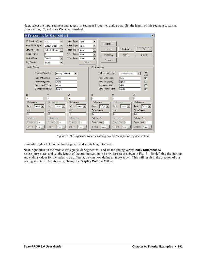
BeamPROP 8.0 User Guide Chapter 9: Tutorial Examples • 191
Next, select the input segment and access its Segment Properties dialog box. Set the length of this segment to Lin as shown in Fig. 2, and click OK when finished.
Figure 2: The Segment Properties dialog box for the input waveguide section.
Similarly, right click on the third segment and set its length to Lout.
Next, right click on the middle waveguide, or Segment #2, and set the ending vertex Index Difference to delta_grating, and set the length of the grating section to be M*Period as shown in Fig. 3. By defining the starting and ending values for the index to be different, we can now define an index taper. This will result in the creation of our grating structure. Additionally, change the Display Color to Yellow.
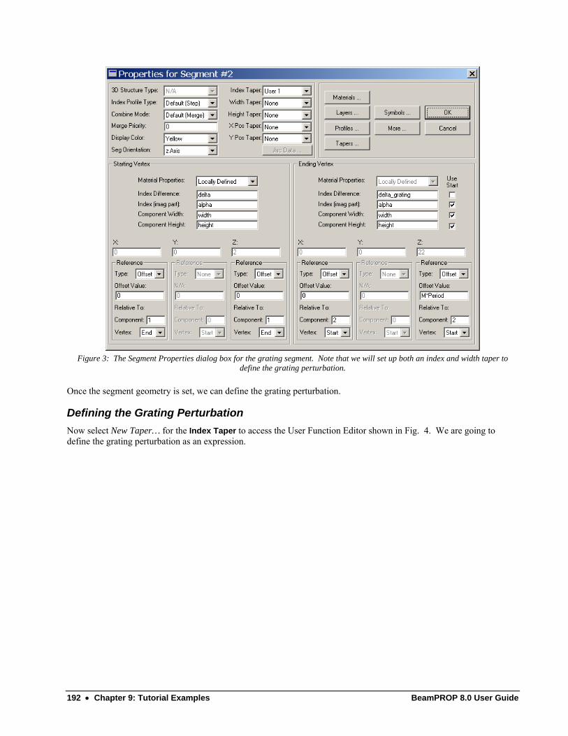
192 • Chapter 9: Tutorial Examples BeamPROP 8.0 User Guide
Figure 3: The Segment Properties dialog box for the grating segment. Note that we will set up both an index and width taper to
define the grating perturbation.
Once the segment geometry is set, we can define the grating perturbation.
Defining the Grating Perturbation Now select New Taper… for the Index Taper to access the User Function Editor shown in Fig. 4. We are going to define the grating perturbation as an expression.
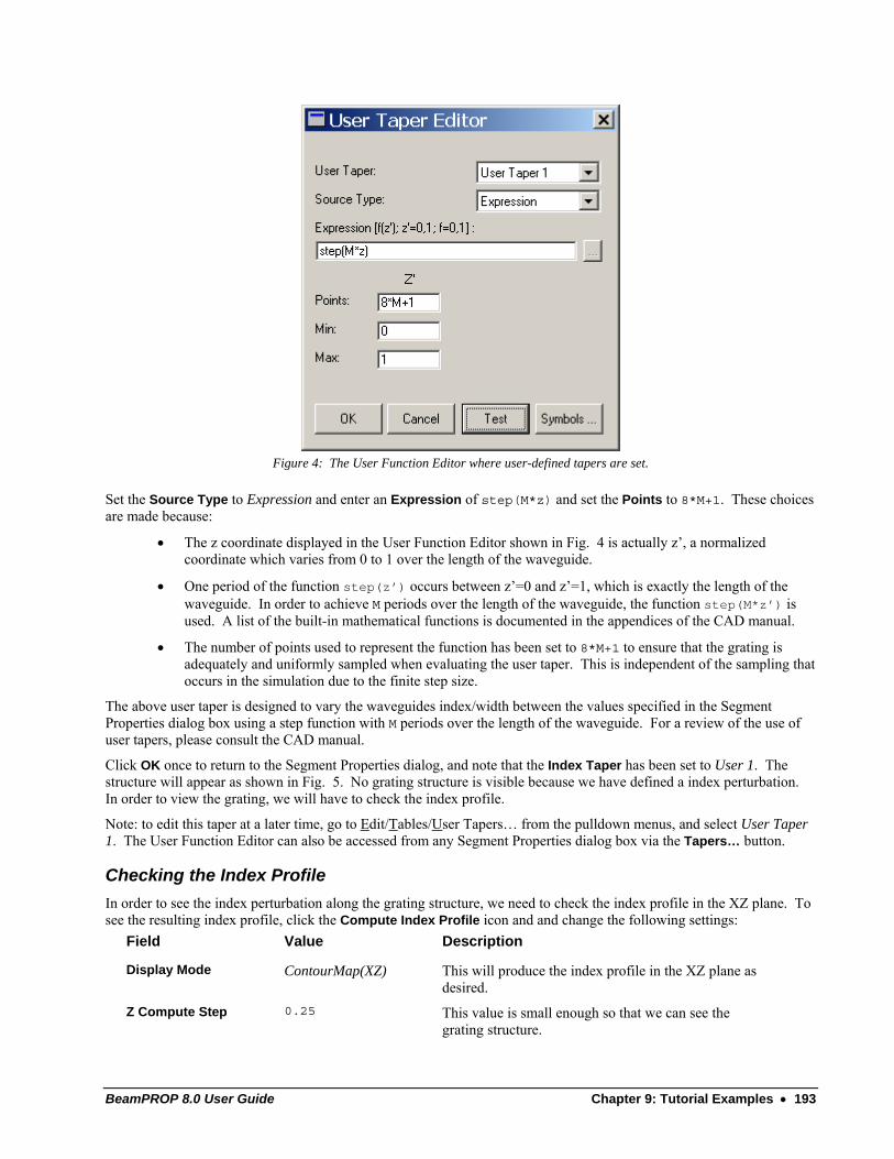
BeamPROP 8.0 User Guide Chapter 9: Tutorial Examples • 193
Figure 4: The User Function Editor where user-defined tapers are set.
Set the Source Type to Expression and enter an Expression of step(M*z) and set the Points to 8*M+1. These choices are made because:
• The z coordinate displayed in the User Function Editor shown in Fig. 4 is actually z’, a normalized coordinate which varies from 0 to 1 over the length of the waveguide.
• One period of the function step(z’) occurs between z’=0 and z’=1, which is exactly the length of the waveguide. In order to achieve M periods over the length of the waveguide, the function step(M*z’) is used. A list of the built-in mathematical functions is documented in the appendices of the CAD manual.
• The number of points used to represent the function has been set to 8*M+1 to ensure that the grating is adequately and uniformly sampled when evaluating the user taper. This is independent of the sampling that occurs in the simulation due to the finite step size.
The above user taper is designed to vary the waveguides index/width between the values specified in the Segment Properties dialog box using a step function with M periods over the length of the waveguide. For a review of the use of user tapers, please consult the CAD manual.
Click OK once to return to the Segment Properties dialog, and note that the Index Taper has been set to User 1. The structure will appear as shown in Fig. 5. No grating structure is visible because we have defined a index perturbation. In order to view the grating, we will have to check the index profile.
Note: to edit this taper at a later time, go to Edit/Tables/User Tapers… from the pulldown menus, and select User Taper 1. The User Function Editor can also be accessed from any Segment Properties dialog box via the Tapers… button.
Checking the Index Profile In order to see the index perturbation along the grating structure, we need to check the index profile in the XZ plane. To see the resulting index profile, click the Compute Index Profile icon and and change the following settings: Field Value Description Display Mode ContourMap(XZ) This will produce the index profile in the XZ plane as
desired. Z Compute Step 0.25 This value is small enough so that we can see the
grating structure.
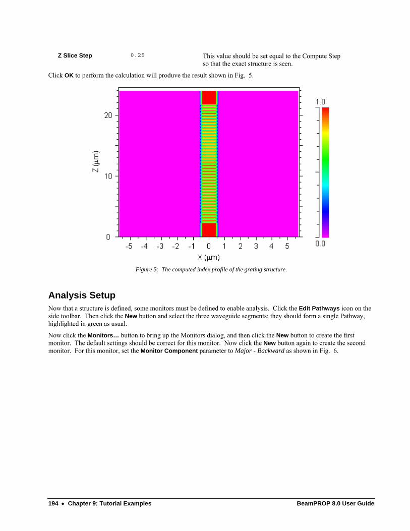
194 • Chapter 9: Tutorial Examples BeamPROP 8.0 User Guide
Z Slice Step 0.25 This value should be set equal to the Compute Step so that the exact structure is seen.
Click OK to perform the calculation will produve the result shown in Fig. 5.
Figure 5: The computed index profile of the grating structure.
Analysis Setup Now that a structure is defined, some monitors must be defined to enable analysis. Click the Edit Pathways icon on the side toolbar. Then click the New button and select the three waveguide segments; they should form a single Pathway, highlighted in green as usual.
Now click the Monitors… button to bring up the Monitors dialog, and then click the New button to create the first monitor. The default settings should be correct for this monitor. Now click the New button again to create the second monitor. For this monitor, set the Monitor Component parameter to Major - Backward as shown in Fig. 6.
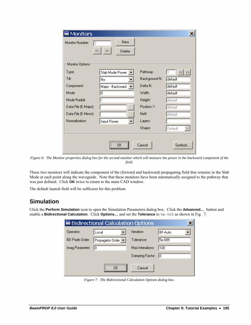
BeamPROP 8.0 User Guide Chapter 9: Tutorial Examples • 195
Figure 6: The Monitor properties dialog box for the second monitor which will measure the power in the backward component of the
field.
These two monitors will indicate the component of the (forward and backward) propagating field that remains in the Slab Mode at each point along the waveguide. Note that these monitors have been automatically assigned to the pathway that was just defined. Click OK twice to return to the main CAD window.
The default launch field will be sufficient for this problem.
Simulation Click the Perform Simulation icon to open the Simulation Parameters dialog box. Click the Advanced… button and enable a Bidirectional Calculation. Click Options… and set the Tolerance to 5e-005 as shown in Fig. 7.
Figure 7: The Bidirectional Calculation Options dialog box.
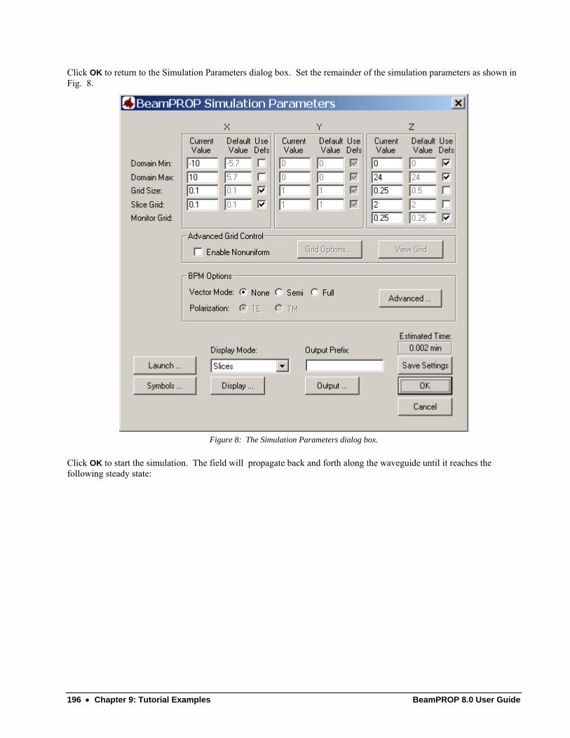
196 • Chapter 9: Tutorial Examples BeamPROP 8.0 User Guide
Click OK to return to the Simulation Parameters dialog box. Set the remainder of the simulation parameters as shown in Fig. 8.
Figure 8: The Simulation Parameters dialog box.
Click OK to start the simulation. The field will propagate back and forth along the waveguide until it reaches the following steady state:
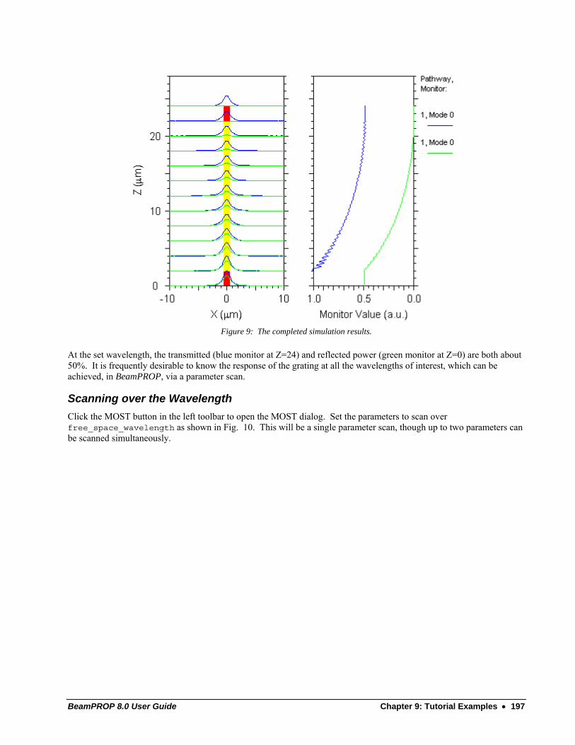
BeamPROP 8.0 User Guide Chapter 9: Tutorial Examples • 197
Figure 9: The completed simulation results.
At the set wavelength, the transmitted (blue monitor at Z=24) and reflected power (green monitor at Z=0) are both about 50%. It is frequently desirable to know the response of the grating at all the wavelengths of interest, which can be achieved, in BeamPROP, via a parameter scan.
Scanning over the Wavelength Click the MOST button in the left toolbar to open the MOST dialog. Set the parameters to scan over free_space_wavelength as shown in Fig. 10. This will be a single parameter scan, though up to two parameters can be scanned simultaneously.
198 • Chapter 9: Tutorial Examples BeamPROP 8.0 User Guide
Figure 10: The Scan Variable dialog box.
Click OK to begin the scan. It will take a few moments; each simulation will flash on the screen in turn. Once it is completed, click the DataBROWSER button to view the results.
Figure 11: The completed scan results.

BeamPROP 8.0 User Guide Chapter 9: Tutorial Examples • 199
For this example, the data points that are collected are, contrary to a non bidirectional scan, taken at the beginning of the structure rather than the end. Thus, the forward power (blue) will always be one, and the reflected spectrum (green) is as one would expect. Note that for the Matrix Iteration methods, the forward power is taken at the end of the structure as usual, and both spectra would be as expected.
Further Exploration Use the Symbol Table to change the value of M and rerun the scan. Observe the change in the width and height of the resonance.

BeamPROP 8.0 User Guide Chapter 9: Tutorial Examples • 201
Tutorial 9 - Using the Electrode Feature The following notes demonstrate an example Mach_Zehnder electro-optical modulator to show how to use the Electrode/Heater Utility in BeamPROP. The associated file for this example is electrode.ind.
Device Layout In the CAD layout window, click on the New Circuit icon in the top toolbar. Enter the information for waveguide as shown in Fig. 1. Set the Model Dimension to 3D and and select Multilayer for the 3D Structure Type.
Figure 1: The Startup Window where the global defaults are set.
Here, a multilayer structure is used to create a 3D channel waveguide. Click the Edit Layers… button, and add a new layer with waveguide height and core index as shown in Fig. 2 using the predefined symbols height, background_index, and delta.
Click the New Layer button to add a new layer. Then enter height in the Height text box, and enter background_index+delta into the Index(real) text box. Finally, press the Accept Layer button, then press OK. Note that the Slab Height equals 0 and the Cover Index equals the background_index are chosen to obtain the channel structure. Finally, press OK to close the startup dialog.
202 • Chapter 9: Tutorial Examples BeamPROP 8.0 User Guide
Figure 2: The Layer Table Editor.
Click the Segment Mode button and draw the input waveguide by holding down the left mouse button, dragging, and then letting go.. Then by right-clicking the waveguide, the properties dialog for this segment can be accessed. The length of input waveguide can be chosen in the dialog by defining a variable Lin = 1000 μm in the symbol table, and then setting the segment properties as shown in Fig. 3. It is usually convenient to set the beginning vertex at x=0 and z=0. You may want to resize the picture and grid by clicking View/Full on the view toolbar.
BeamPROP 8.0 User Guide Chapter 9: Tutorial Examples • 203
Figure 3: The Segment Properties dialog box for the straight input waveguide segment.
Now we will draw the S-bends. Select S-bend Mode from the left tool bar and click the left mouse button near the end of the first segment and drag it to the side. In this way, the beginning vertex of this segment is automatically connected to the ending vertex of the first segment. Then right click the s-bend segment. Click on the Symbols… button. The create several new variables: Sep = 20 and Lbend = 2000. Sep will be the separation between the two arms of the Mach-Zehnder modulator and Lbend will be the length of the S-bend.
Click OK to leave the Symbol Table Editor. Back in the properties dialog, set the following parameters as shown in Fig. 4. For the Ending Vertex, change the X Offset Value to Sep/2. The Z Offset Value should be set to Lbend. By the same procedure, the left S-Band can be drawn with the exact same parameters except the Ending Vertex, X Offset Value should be set to –Sep/2. Click OK to leave the properties dialog.
204 • Chapter 9: Tutorial Examples BeamPROP 8.0 User Guide
Figure 4: The Segment Properties dialog box for one of the S-bend segments.
Next, define a variable Larm equal to 4000 in the symbol table. Click on the Segment Mode button on the left and then draw two straight waveguides connected to the two s-bends. Set their Ending Vertex, Z Offset Value to Larm.
Draw two output S-bends. For each output S-bend, set the Ending Vertex, X Offset Value to 0. Also, make sure it is referenced to the ending vertex of component 1. Then, set the Z Offset Value to Lbend. This can all be seen in Fig. 5.
BeamPROP 8.0 User Guide Chapter 9: Tutorial Examples • 205
Figure 5: The Segment Properties dialog for one of the S-bend segments.
Next, draw a straight waveguide at the end of the current structure. This waveguide will be tapered to cutoff the antisymmetric mode of the Mach-Zehnder. To do this, define Wout = 4 and Ltaper = 1000 in the symbol table, and set the properties of the straight waveguide just drawn as shown in Fig. 6.
206 • Chapter 9: Tutorial Examples BeamPROP 8.0 User Guide
Figure 6: The Segment Properties for the tapered output waveguide segment.
Finally, draw the output straight waveguide and set its length to Lout, analogously to the input waveguide, and set its starting and ending width to Wout.
The final drawing, as of now, should look like Fig. 7.
BeamPROP 8.0 User Guide Chapter 9: Tutorial Examples • 207
Figure 7: The completed structure as seen in the CAD window in multi=pane mode.
Electrode Layer and Electrode Setup and Simulation A simple multilayer geometry for the electrode calculation can be constructed via the Edit/Tables/Edit-Electrode/Heater-Layers menu. For each layer, the layer thickness, dielectric constant and electro-optic coefficient can be defined for the electrical field calculation.
Creating Electrodes First, go to the Electrode/Heater Layer Table Editor and then press Symbols… Create the new variables Eps, equal to background_index^2, and Rcoef, equal to 0.0008. A detailed explanation for these parameters can be found in Section 7.F. Press OK to go back to the Electrode/Heater Layer Table Editor.
Now, enter the layers as shown in Fig. 8 by first pressing New, then entering the info, and then pressing Accept for each layer. Note that the substrate is layer 0 and at the top of layer 0, Y=0. Press OK to leave the Electrode/Heater Layer Table Editor.
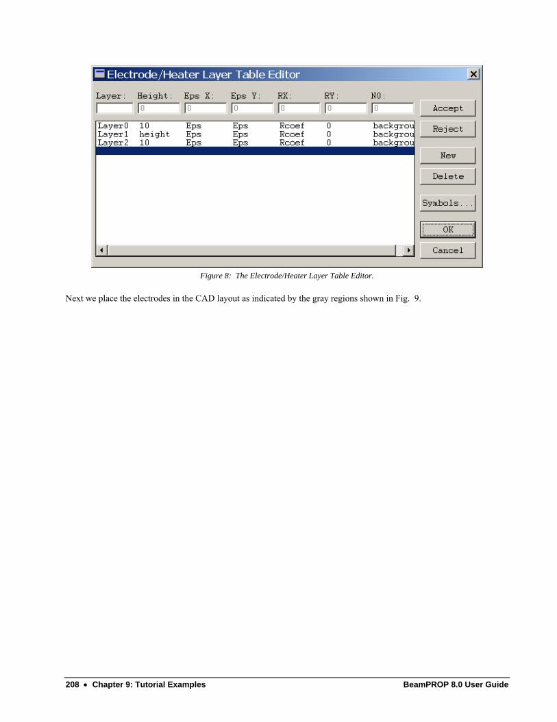
208 • Chapter 9: Tutorial Examples BeamPROP 8.0 User Guide
Figure 8: The Electrode/Heater Layer Table Editor.
Next we place the electrodes in the CAD layout as indicated by the gray regions shown in Fig. 9.
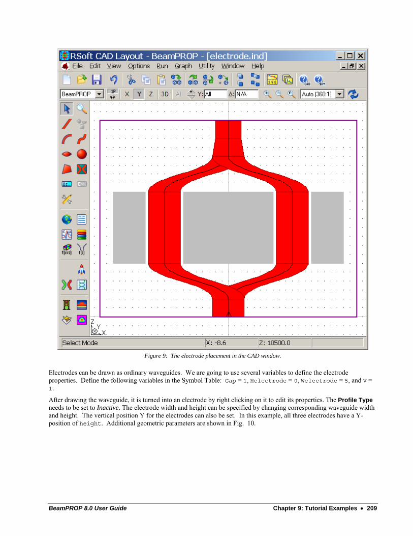
BeamPROP 8.0 User Guide Chapter 9: Tutorial Examples • 209
Figure 9: The electrode placement in the CAD window.
Electrodes can be drawn as ordinary waveguides. We are going to use several variables to define the electrode properties. Define the following variables in the Symbol Table: Gap = 1, Helectrode = 0, Welectrode = 5, and V = 1.
After drawing the waveguide, it is turned into an electrode by right clicking on it to edit its properties. The Profile Type needs to be set to Inactive. The electrode width and height can be specified by changing corresponding waveguide width and height. The vertical position Y for the electrodes can also be set. In this example, all three electrodes have a Y-position of height. Additional geometric parameters are shown in Fig. 10.
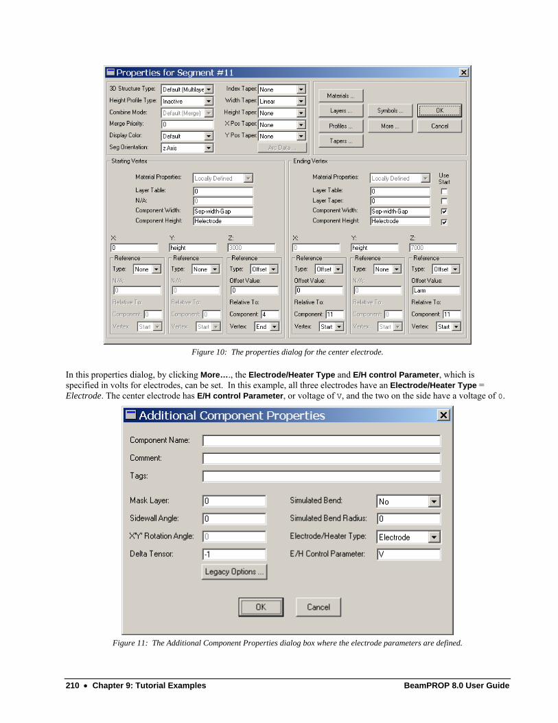
210 • Chapter 9: Tutorial Examples BeamPROP 8.0 User Guide
Figure 10: The properties dialog for the center electrode.
In this properties dialog, by clicking More…., the Electrode/Heater Type and E/H control Parameter, which is specified in volts for electrodes, can be set. In this example, all three electrodes have an Electrode/Heater Type = Electrode. The center electrode has E/H control Parameter, or voltage of V, and the two on the side have a voltage of 0.
Figure 11: The Additional Component Properties dialog box where the electrode parameters are defined.
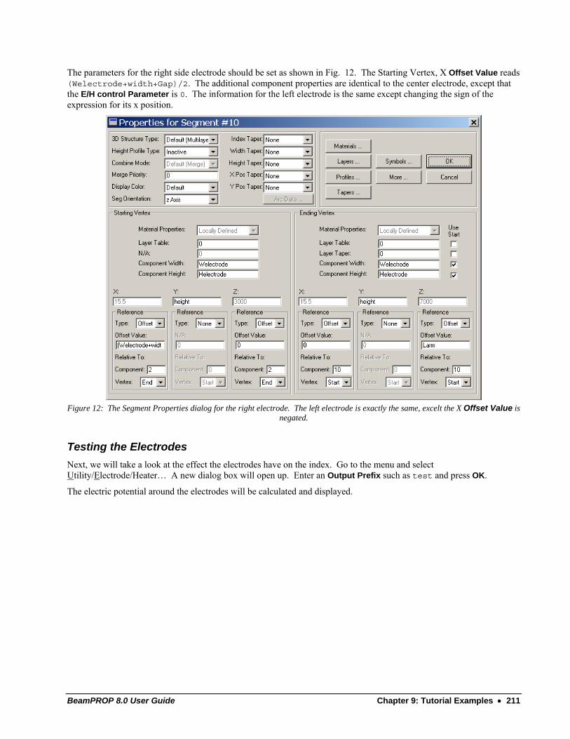
BeamPROP 8.0 User Guide Chapter 9: Tutorial Examples • 211
The parameters for the right side electrode should be set as shown in Fig. 12. The Starting Vertex, X Offset Value reads (Welectrode+width+Gap)/2. The additional component properties are identical to the center electrode, except that the E/H control Parameter is 0. The information for the left electrode is the same except changing the sign of the expression for its x position.
Figure 12: The Segment Properties dialog for the right electrode. The left electrode is exactly the same, excelt the X Offset Value is
negated.
Testing the Electrodes Next, we will take a look at the effect the electrodes have on the index. Go to the menu and select Utility/Electrode/Heater… A new dialog box will open up. Enter an Output Prefix such as test and press OK.
The electric potential around the electrodes will be calculated and displayed.
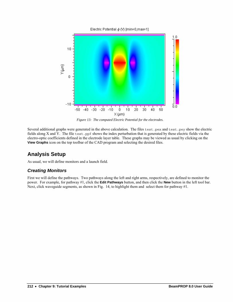
212 • Chapter 9: Tutorial Examples BeamPROP 8.0 User Guide
Figure 13: The computed Electric Potential for the electrodes.
Several additional graphs were generated in the above calculation. The files test.pex and test.pey show the electric fields along X and Y. The file test.ppf shows the index perturbation that is generated by these electric fields via the electro-optic coefficients defined in the electrode layer table. These graphs may be viewed as usual by clicking on the View Graphs icon on the top toolbar of the CAD program and selecting the desired files.
Analysis Setup As usual, we will define monitors and a launch field.
Creating Monitors First we will define the pathways. Two pathways along the left and right arms, respectively, are defined to monitor the power. For example, for pathway #1, click the Edit Pathways button, and then click the New button in the left tool bar. Next, click waveguide segments, as shown in Fig. 14, to highlight them and select them for pathway #1.
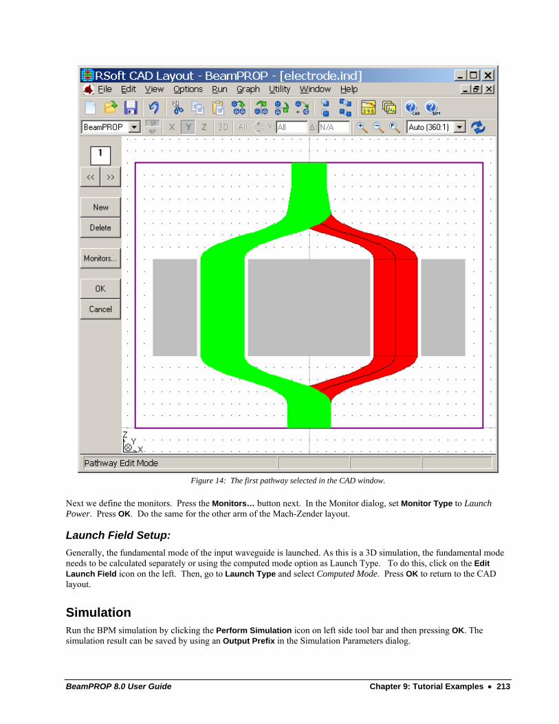
BeamPROP 8.0 User Guide Chapter 9: Tutorial Examples • 213
Figure 14: The first pathway selected in the CAD window.
Next we define the monitors. Press the Monitors… button next. In the Monitor dialog, set Monitor Type to Launch Power. Press OK. Do the same for the other arm of the Mach-Zender layout.
Launch Field Setup: Generally, the fundamental mode of the input waveguide is launched. As this is a 3D simulation, the fundamental mode needs to be calculated separately or using the computed mode option as Launch Type. To do this, click on the Edit Launch Field icon on the left. Then, go to Launch Type and select Computed Mode. Press OK to return to the CAD layout.
Simulation Run the BPM simulation by clicking the Perform Simulation icon on left side tool bar and then pressing OK. The simulation result can be saved by using an Output Prefix in the Simulation Parameters dialog.
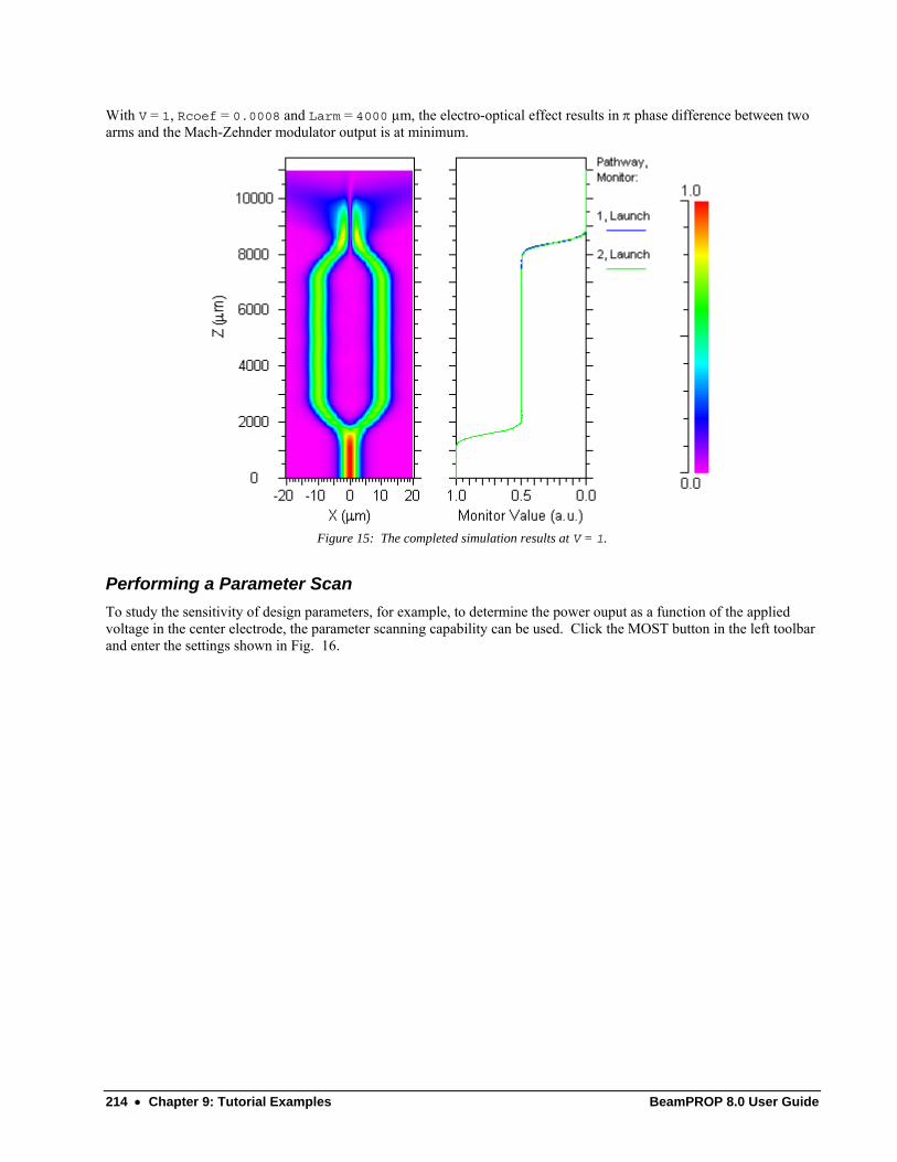
214 • Chapter 9: Tutorial Examples BeamPROP 8.0 User Guide
With V = 1, Rcoef = 0.0008 and Larm = 4000 µm, the electro-optical effect results in π phase difference between two arms and the Mach-Zehnder modulator output is at minimum.
Figure 15: The completed simulation results at V = 1.
Performing a Parameter Scan To study the sensitivity of design parameters, for example, to determine the power ouput as a function of the applied voltage in the center electrode, the parameter scanning capability can be used. Click the MOST button in the left toolbar and enter the settings shown in Fig. 16.
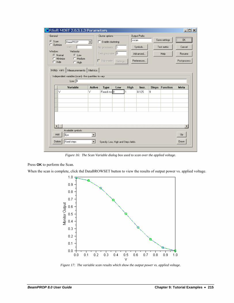
BeamPROP 8.0 User Guide Chapter 9: Tutorial Examples • 215
Figure 16: The Scan Variable dialog box used to scan over the applied voltage.
Press OK to perform the Scan.
When the scan is complete, click thd DataBROWSET button to view the results of output power vs. applied voltage.
Figure 17: The variable scan results which show the output power vs. applied voltage.


BeamPROP 8.0 User Guide Chapter 9: Tutorial Examples • 217
Tutorial 10 - Using The WDM Router (AWG) Utility The tutorial on AWG design has been relocated to a different document which consolidates the tutorial and other information on AWG design in a single location. Please refer to the online help located under the CAD Help menu for information about the AWG Utility.

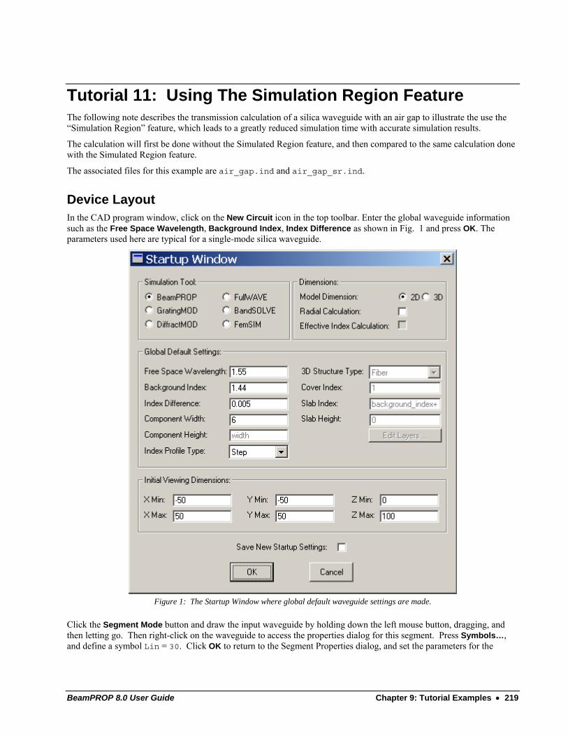
BeamPROP 8.0 User Guide Chapter 9: Tutorial Examples • 219
Tutorial 11: Using The Simulation Region Feature The following note describes the transmission calculation of a silica waveguide with an air gap to illustrate the use the “Simulation Region” feature, which leads to a greatly reduced simulation time with accurate simulation results.
The calculation will first be done without the Simulated Region feature, and then compared to the same calculation done with the Simulated Region feature.
The associated files for this example are air_gap.ind and air_gap_sr.ind.
Device Layout In the CAD program window, click on the New Circuit icon in the top toolbar. Enter the global waveguide information such as the Free Space Wavelength, Background Index, Index Difference as shown in Fig. 1 and press OK. The parameters used here are typical for a single-mode silica waveguide.
Figure 1: The Startup Window where global default waveguide settings are made.
Click the Segment Mode button and draw the input waveguide by holding down the left mouse button, dragging, and then letting go. Then right-click on the waveguide to access the properties dialog for this segment. Press Symbols…, and define a symbol Lin = 30. Click OK to return to the Segment Properties dialog, and set the parameters for the
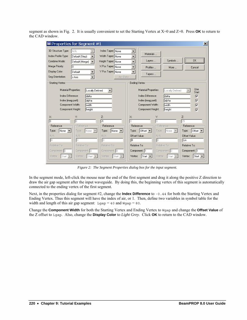
220 • Chapter 9: Tutorial Examples BeamPROP 8.0 User Guide
segment as shown in Fig. 2. It is usually convenient to set the Starting Vertex at X=0 and Z=0. Press OK to return to the CAD window.
Figure 2: The Segment Properties dialog box for the input segment.
In the segment mode, left-click the mouse near the end of the first segment and drag it along the positive Z direction to draw the air gap segment after the input waveguide. By doing this, the beginning vertex of this segment is automatically connected to the ending vertex of the first segment.
Next, in the properties dialog for segment #2, change the Index Difference to -0.44 for both the Starting Vertex and Ending Vertex. Thus this segment will have the index of air, or 1. Then, define two variables in symbol table for the width and length of this air gap segment: Lgap = 40 and Wgap = 80.
Change the Component Width for both the Starting Vertex and Ending Vertex to Wgap and change the Offset Value of the Z offset to Lgap. Also, change the Display Color to Light Grey. Click OK to return to the CAD window.
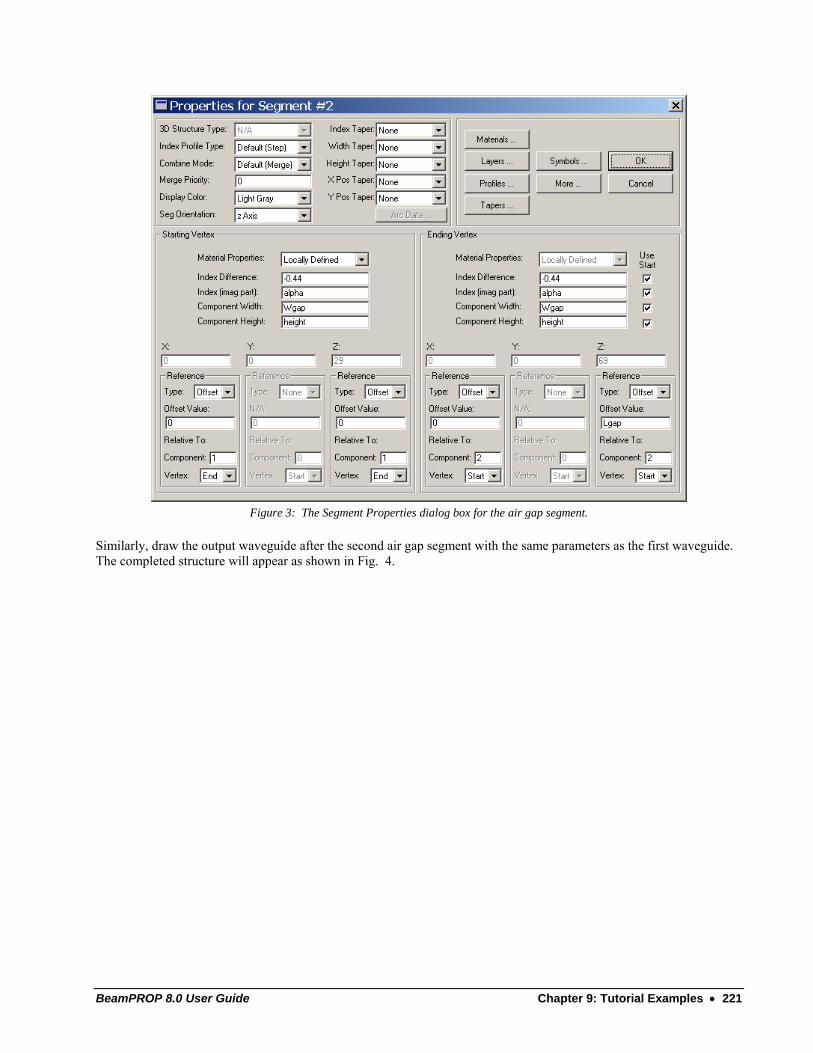
BeamPROP 8.0 User Guide Chapter 9: Tutorial Examples • 221
Figure 3: The Segment Properties dialog box for the air gap segment.
Similarly, draw the output waveguide after the second air gap segment with the same parameters as the first waveguide. The completed structure will appear as shown in Fig. 4.
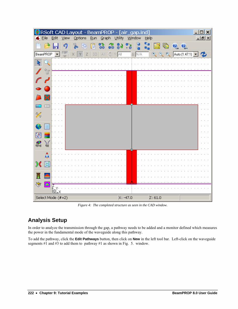
222 • Chapter 9: Tutorial Examples BeamPROP 8.0 User Guide
Figure 4: The completed structure as seen in the CAD window.
Analysis Setup In order to analyze the transmission through the gap, a pathway needs to be added and a monitor defined which measures the power in the fundamental mode of the waveguide along this pathway.
To add the pathway, click the Edit Pathways button, then click on New in the left tool bar. Left-click on the waveguide segments #1 and #3 to add them to pathway #1 as shown in Fig. 5. window.
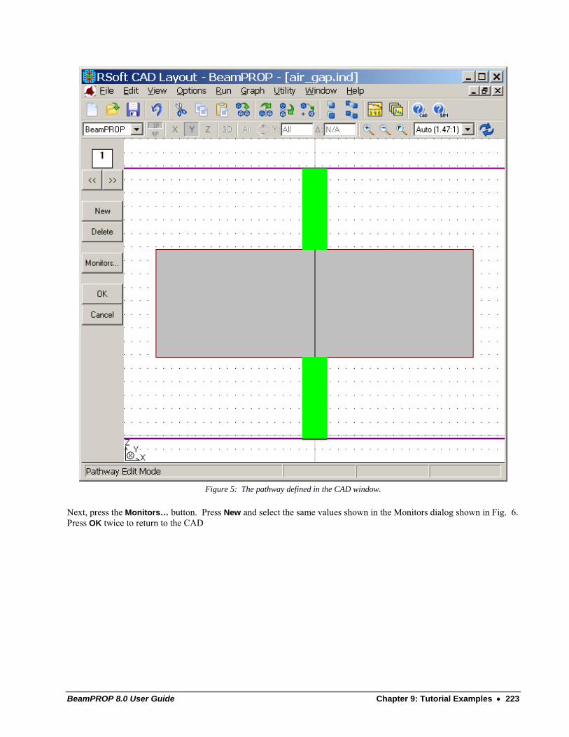
BeamPROP 8.0 User Guide Chapter 9: Tutorial Examples • 223
Figure 5: The pathway defined in the CAD window.
Next, press the Monitors… button. Press New and select the same values shown in the Monitors dialog shown in Fig. 6. Press OK twice to return to the CAD
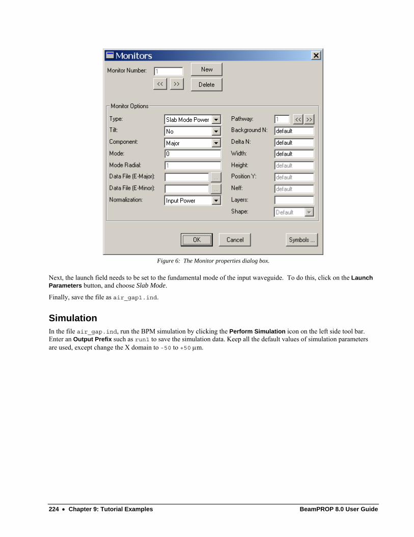
224 • Chapter 9: Tutorial Examples BeamPROP 8.0 User Guide
Figure 6: The Monitor properties dialog box.
Next, the launch field needs to be set to the fundamental mode of the input waveguide. To do this, click on the Launch Parameters button, and choose Slab Mode.
Finally, save the file as air_gap1.ind.
Simulation In the file air_gap.ind, run the BPM simulation by clicking the Perform Simulation icon on the left side tool bar. Enter an Output Prefix such as run1 to save the simulation data. Keep all the default values of simulation parameters are used, except change the X domain to -50 to +50 μm.
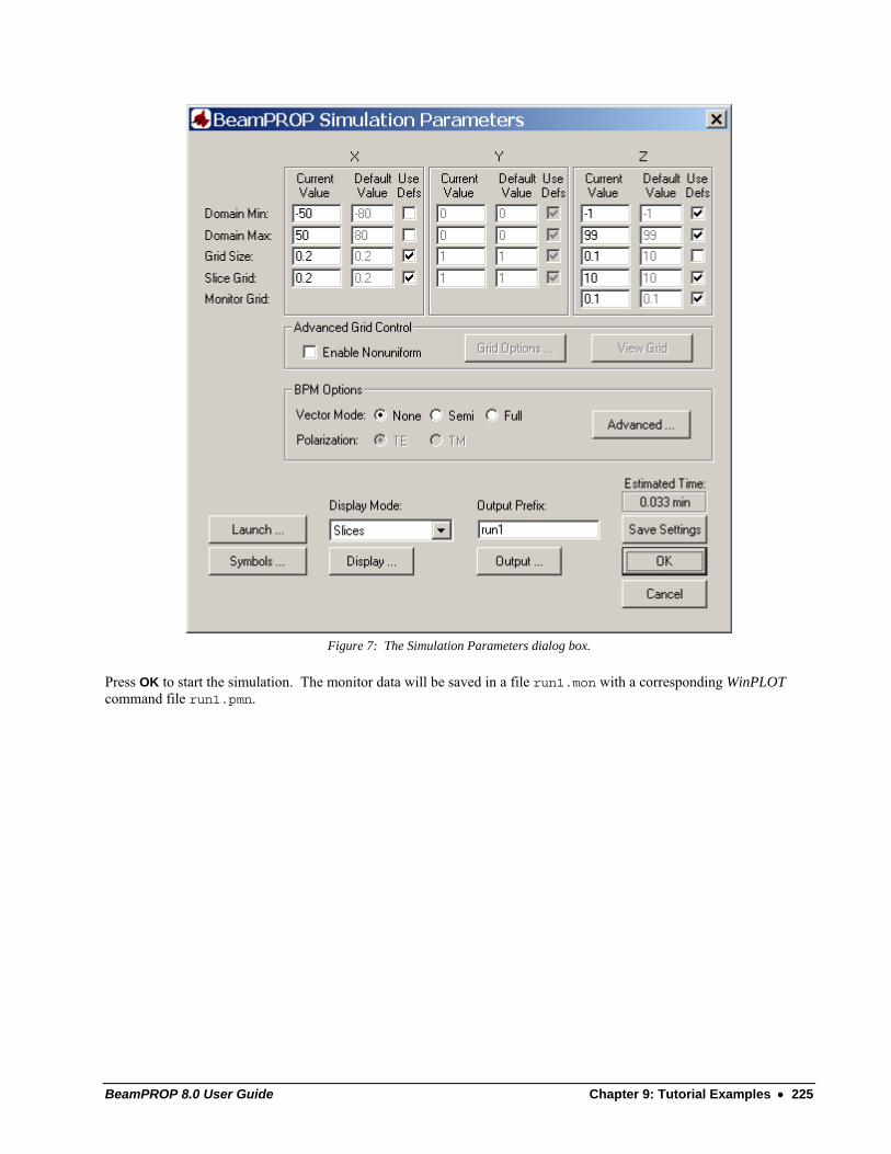
BeamPROP 8.0 User Guide Chapter 9: Tutorial Examples • 225
Figure 7: The Simulation Parameters dialog box.
Press OK to start the simulation. The monitor data will be saved in a file run1.mon with a corresponding WinPLOT command file run1.pmn.
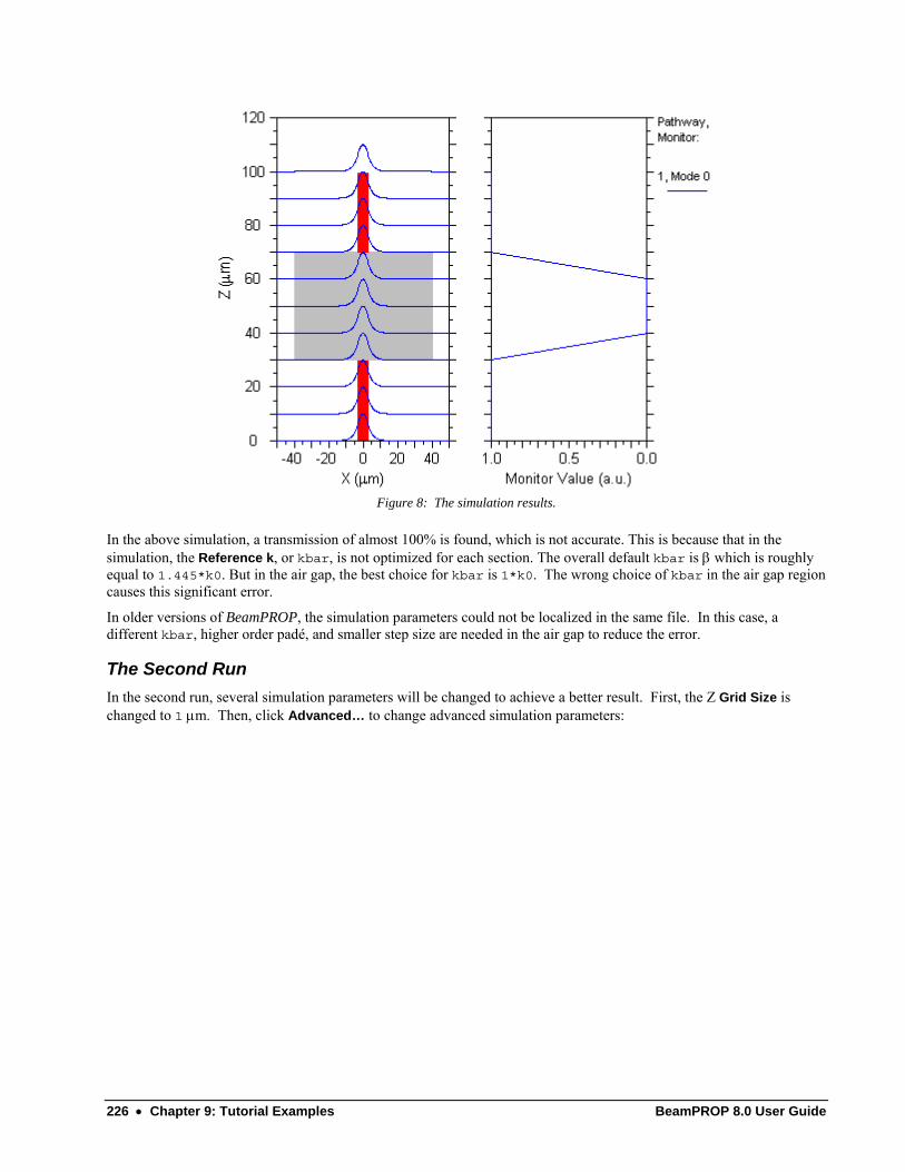
226 • Chapter 9: Tutorial Examples BeamPROP 8.0 User Guide
Figure 8: The simulation results.
In the above simulation, a transmission of almost 100% is found, which is not accurate. This is because that in the simulation, the Reference k, or kbar, is not optimized for each section. The overall default kbar is β which is roughly equal to 1.445*k0. But in the air gap, the best choice for kbar is 1*k0. The wrong choice of kbar in the air gap region causes this significant error.
In older versions of BeamPROP, the simulation parameters could not be localized in the same file. In this case, a different kbar, higher order padé, and smaller step size are needed in the air gap to reduce the error.
The Second Run In the second run, several simulation parameters will be changed to achieve a better result. First, the Z Grid Size is changed to 1 μm. Then, click Advanced… to change advanced simulation parameters:
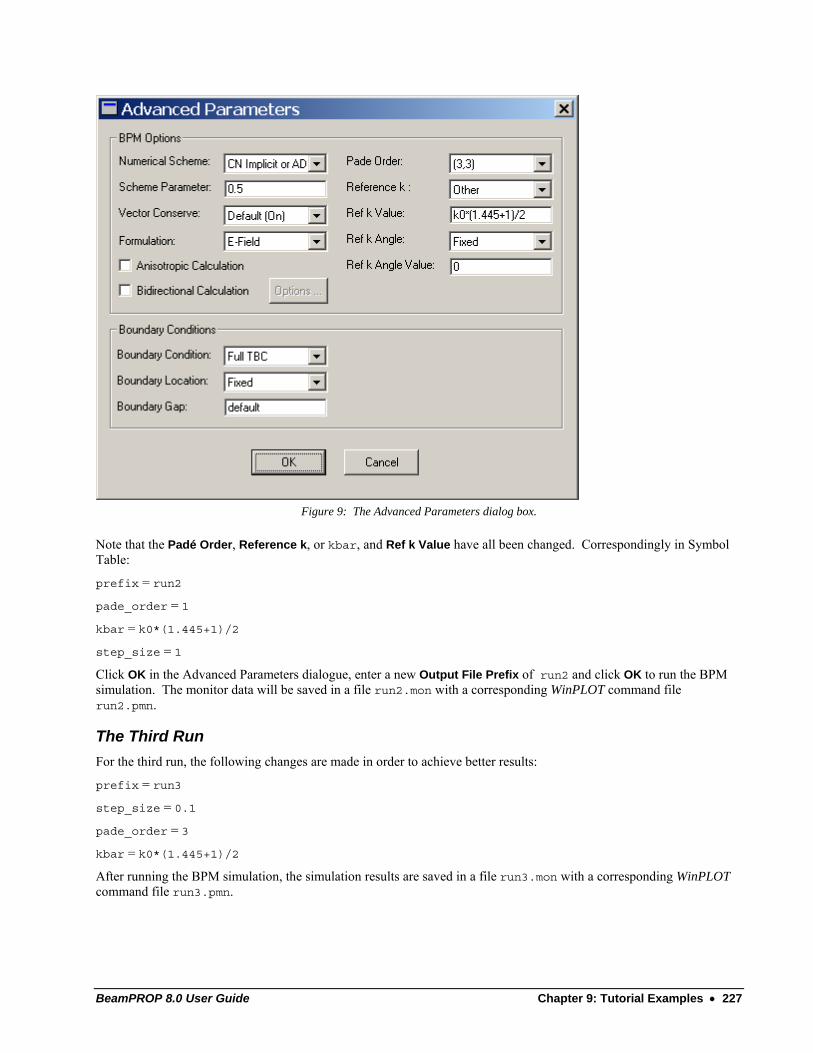
BeamPROP 8.0 User Guide Chapter 9: Tutorial Examples • 227
Figure 9: The Advanced Parameters dialog box.
Note that the Padé Order, Reference k, or kbar, and Ref k Value have all been changed. Correspondingly in Symbol Table:
prefix = run2
pade_order = 1
kbar = k0*(1.445+1)/2
step_size = 1
Click OK in the Advanced Parameters dialogue, enter a new Output File Prefix of run2 and click OK to run the BPM simulation. The monitor data will be saved in a file run2.mon with a corresponding WinPLOT command file run2.pmn.
The Third Run For the third run, the following changes are made in order to achieve better results:
prefix = run3
step_size = 0.1
pade_order = 3
kbar = k0*(1.445+1)/2
After running the BPM simulation, the simulation results are saved in a file run3.mon with a corresponding WinPLOT command file run3.pmn.
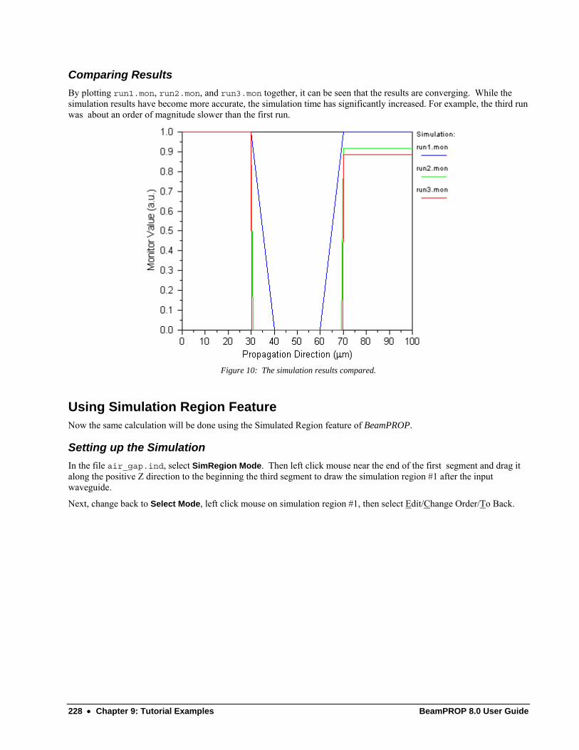
228 • Chapter 9: Tutorial Examples BeamPROP 8.0 User Guide
Comparing Results By plotting run1.mon, run2.mon, and run3.mon together, it can be seen that the results are converging. While the simulation results have become more accurate, the simulation time has significantly increased. For example, the third run was about an order of magnitude slower than the first run.
Figure 10: The simulation results compared.
Using Simulation Region Feature Now the same calculation will be done using the Simulated Region feature of BeamPROP.
Setting up the Simulation In the file air_gap.ind, select SimRegion Mode. Then left click mouse near the end of the first segment and drag it along the positive Z direction to the beginning the third segment to draw the simulation region #1 after the input waveguide.
Next, change back to Select Mode, left click mouse on simulation region #1, then select Edit/Change Order/To Back.
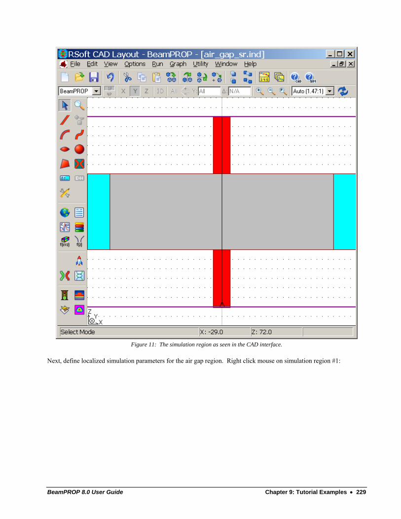
BeamPROP 8.0 User Guide Chapter 9: Tutorial Examples • 229
Figure 11: The simulation region as seen in the CAD interface.
Next, define localized simulation parameters for the air gap region. Right click mouse on simulation region #1:

230 • Chapter 9: Tutorial Examples BeamPROP 8.0 User Guide
Figure 12: The Properties dialog box for the Simulation Region
Click the Local Symbols… button and input the following variables and corresponding values: Variable Value Value free_space_wavelength 1.55
k0 (2*pi)/free_space_wavelength
kbar k0*1
pade_order 1
step_size 1
Note that different pade_order, kbar and step_size from the Global Symbol Table are used here.
These variables in the Local Symbol Table are just like the normal, Global Symbol Table, which is also accessible in the simulation region properties dialog; however variables defined in the local symbol table override those in the global table. Currently, the only variables which can be overridden are: Variable Description step_size Z Grid Size kbar Rreference k kbar_angle Reference k Angle pade_order Padé Order(0-4) simulated_bend Enable/disable Simulated Bend (0/1) simulated_bend_radius Set Simulated Bend Radius (can be +/-) scheme Set Simulation Method (SCHEME_CN,...)
Click OK and save this file as air_gap_sr.ind. Change the Output Prefix to run_sr1 and run the BPM simulation. The simulation results, will be saved in a file run_sr1.mon with a corresponding WinPLOT command file run_sr1.pmn.
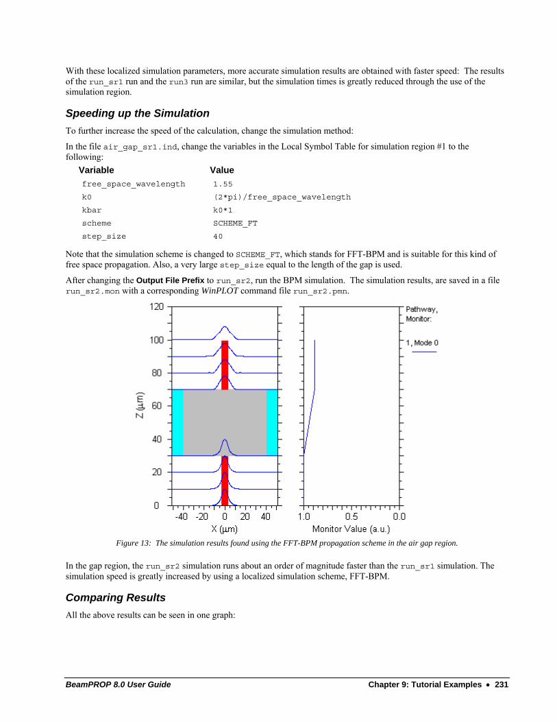
BeamPROP 8.0 User Guide Chapter 9: Tutorial Examples • 231
With these localized simulation parameters, more accurate simulation results are obtained with faster speed: The results of the run_sr1 run and the run3 run are similar, but the simulation times is greatly reduced through the use of the simulation region.
Speeding up the Simulation To further increase the speed of the calculation, change the simulation method:
In the file air_gap_sr1.ind, change the variables in the Local Symbol Table for simulation region #1 to the following: Variable Value free_space_wavelength 1.55
k0 (2*pi)/free_space_wavelength
kbar k0*1
scheme SCHEME_FT
step_size 40
Note that the simulation scheme is changed to SCHEME_FT, which stands for FFT-BPM and is suitable for this kind of free space propagation. Also, a very large step_size equal to the length of the gap is used.
After changing the Output File Prefix to run_sr2, run the BPM simulation. The simulation results, are saved in a file run_sr2.mon with a corresponding WinPLOT command file run_sr2.pmn.
Figure 13: The simulation results found using the FFT-BPM propagation scheme in the air gap region.
In the gap region, the run_sr2 simulation runs about an order of magnitude faster than the run_sr1 simulation. The simulation speed is greatly increased by using a localized simulation scheme, FFT-BPM.
Comparing Results All the above results can be seen in one graph:
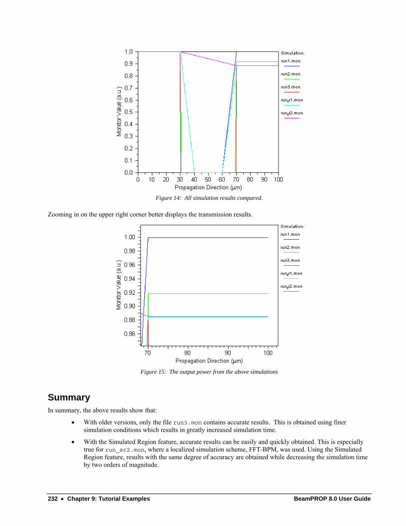
232 • Chapter 9: Tutorial Examples BeamPROP 8.0 User Guide
Figure 14: All simulation results compared.
Zooming in on the upper right corner better displays the transmission results.
Figure 15: The output power from the above simulations
Summary In summary, the above results show that:
• With older versions, only the file run3.mon contains accurate results. This is obtained using finer simulation conditions which results in greatly increased simulation time.
• With the Simulated Region feature, accurate results can be easily and quickly obtained. This is especially true for run_sr2.mon, where a localized simulation scheme, FFT-BPM, was used. Using the Simulated Region feature, results with the same degree of accuracy are obtained while decreasing the simulation time by two orders of magnitude.

BeamPROP 8.0 User Guide Chapter 9: Tutorial Examples • 233
References [1] L. B. Soldano and E. C. M. Pennings, “Optical multi-mode interference devices based on self-imaging: Principles and applications,” J. Lightwave Technol., 13, 615 (1995)

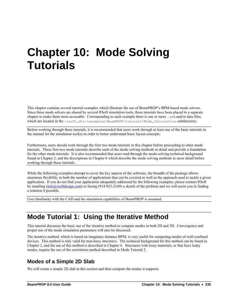
BeamPROP 8.0 User Guide Chapter 10: Mode Solving Tutorials • 235
Chapter 10: Mode Solving Tutorials
This chapter contains several tutorial examples which illustrate the use of BeamPROP’s BPM-based mode solvers. Since these mode solvers are shared by several RSoft simulation tools, these tutorials have been placed in a separate chapter to make them more accusable. Corresponding to each example there is one or more .ind and/or data files, which are located in the <rsoft_dir>\examples\BeamPROP\tutorial\Mode_Calculation subdirectory.
Before working through these tutorials, it is recommended that users work through at least one of the basic tutorials in the manual for the simulation tool(s) in order to better understand basic layout concepts.
Furthermore, users should work through the first two mode tutorials in this chapter before proceeding to other mode tutorials. These first two mode tutorials describe each of the mode solving methods in detail and provide a foundation for the other mode tutorials. It is also recommended that users read through the mode-solving technical background found in Chapter 2, and the descriptions in Chapter 6 which describe the mode solving methods in more detail before working through these tutorials.
While the following examples attempt to cover the key aspects of the software, the breadth of the package allows enormous flexibility in both the number of applications that can be covered as well as the approach used to tackle a given application. If you do not find your application adequately addressed by the following examples, please contact RSoft by emailing ([email protected]) or faxing (914-923-2169) a sketch of the problem and we will assist you in finding a solution if possible.
User familiarity with the CAD and the simulation capabilities of BeamPROP is assumed.
Mode Tutorial 1: Using the Iterative Method This tutorial discusses the basic use of the iterative method to compute modes in both 2D and 3D. Convergence and proper use of the mode simulation parameters will also be discussed.
The iterative method, which is based on imaginary distance BPM, is very useful for computing modes of well-confined devices. This method is only valid for non-lossy structures. The technical background for this method can be found in Chapter 2, and the use of this method is described in Chapter 6. Structures with lossy materials, or that have leaky modes, require the use of the correlation method described in Mode Tutorial 2.
Modes of a Simple 2D Slab We will create a simple 2D slab in this section and then compute the modes it supports.
236 • Chapter 10: Mode Solving Tutorials BeamPROP 8.0 User Guide
Creating the Structure Click the New Circuit button in the CAD window and set the following parameters: Parameter Value Description
Free Space Wavelength 1.55 Sets the simulation wavelength.
Background Index 1.0 This represents the real refractive index of the background material where no structure has been defined.
Index Difference 0.2 This represents the default difference between a component and the background material. In this case this means that the structure will have an index of 1.2.
Once these settings are made, click OK to continue.
In the CAD, draw a straight waveguide segment from (X,Z) = (0,0) to (0,1000). The structure length, in this case 1000 µm, need only be long enough to allow the mode solver to converge. In this case a warning will be displayed and the user should lengthen the structure and retry the simulation.
The index profile of the structure can be computed by click the Display Index Profile in the CAD.
Figure 1: The computed index profile of the simple 2D slab.
Launch Settings The use of an appropriate launch field is critical when computing modes. It is important to excite all the modes of the structure in order to properly compute them. If a particular launch field does not excite a particular mode, the mode solvers will not compute it. As a general rule, a offset Gaussian launch field is usually sufficient to excite a large continuum of modes, including any anti-symmetric modes.
To use an offset Gaussian launch field, click the Edit Launch Field icon in the CAD window. Set the Type to Gaussian and the Position X to be 0.5. Press OK to return to the CAD.
Computing the Fundamental Mode To compute the fundamental mode, click the Compute Modes icon on the left toolbar in the CAD window. This dialog allows the user to set the computation parameters for the mode calculation. The mode method, which is the iterative method described in this tutorial by default, can be chosen via the Mode Options… button. For this example use the
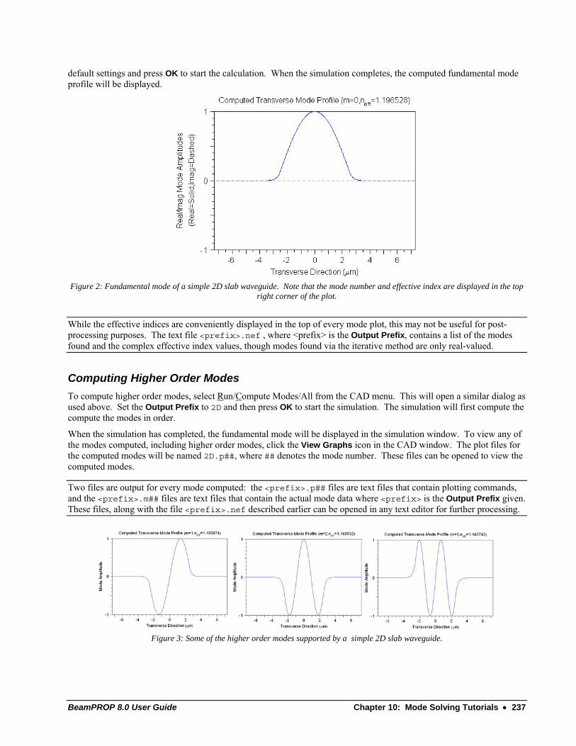
BeamPROP 8.0 User Guide Chapter 10: Mode Solving Tutorials • 237
default settings and press OK to start the calculation. When the simulation completes, the computed fundamental mode profile will be displayed.
Figure 2: Fundamental mode of a simple 2D slab waveguide. Note that the mode number and effective index are displayed in the top
right corner of the plot.
While the effective indices are conveniently displayed in the top of every mode plot, this may not be useful for post-processing purposes. The text file <prefix>.nef , where <prefix> is the Output Prefix, contains a list of the modes found and the complex effective index values, though modes found via the iterative method are only real-valued.
Computing Higher Order Modes To compute higher order modes, select Run/Compute Modes/All from the CAD menu. This will open a similar dialog as used above. Set the Output Prefix to 2D and then press OK to start the simulation. The simulation will first compute the compute the modes in order.
When the simulation has completed, the fundamental mode will be displayed in the simulation window. To view any of the modes computed, including higher order modes, click the View Graphs icon in the CAD window. The plot files for the computed modes will be named 2D.p##, where ## denotes the mode number. These files can be opened to view the computed modes.
Two files are output for every mode computed: the <prefix>.p## files are text files that contain plotting commands, and the <prefix>.m## files are text files that contain the actual mode data where <prefix> is the Output Prefix given. These files, along with the file <prefix>.nef described earlier can be opened in any text editor for further processing.
Figure 3: Some of the higher order modes supported by a simple 2D slab waveguide.
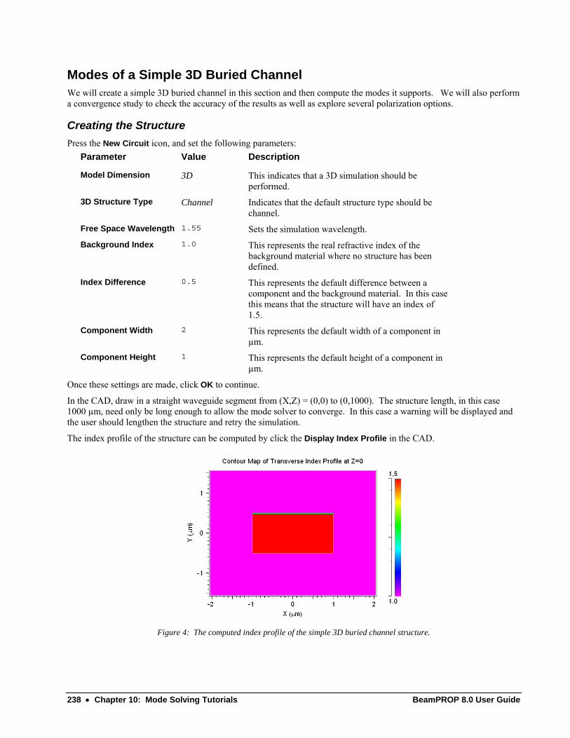
238 • Chapter 10: Mode Solving Tutorials BeamPROP 8.0 User Guide
Modes of a Simple 3D Buried Channel We will create a simple 3D buried channel in this section and then compute the modes it supports. We will also perform a convergence study to check the accuracy of the results as well as explore several polarization options.
Creating the Structure Press the New Circuit icon, and set the following parameters: Parameter Value Description
Model Dimension 3D This indicates that a 3D simulation should be performed.
3D Structure Type Channel Indicates that the default structure type should be channel.
Free Space Wavelength 1.55 Sets the simulation wavelength.
Background Index 1.0 This represents the real refractive index of the background material where no structure has been defined.
Index Difference 0.5 This represents the default difference between a component and the background material. In this case this means that the structure will have an index of 1.5.
Component Width 2 This represents the default width of a component in µm.
Component Height 1 This represents the default height of a component in µm.
Once these settings are made, click OK to continue.
In the CAD, draw in a straight waveguide segment from (X,Z) = (0,0) to (0,1000). The structure length, in this case 1000 µm, need only be long enough to allow the mode solver to converge. In this case a warning will be displayed and the user should lengthen the structure and retry the simulation.
The index profile of the structure can be computed by click the Display Index Profile in the CAD.
Figure 4: The computed index profile of the simple 3D buried channel structure.
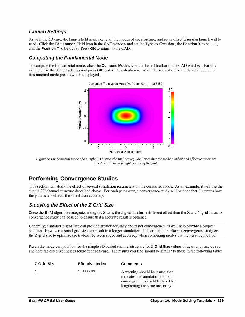
BeamPROP 8.0 User Guide Chapter 10: Mode Solving Tutorials • 239
Launch Settings As with the 2D case, the launch field must excite all the modes of the structure, and so an offset Gaussian launch will be used. Click the Edit Launch Field icon in the CAD window and set the Type to Gaussian , the Position X to be 0.1, and the Position Y to be 0.05. Press OK to return to the CAD.
Computing the Fundamental Mode To compute the fundamental mode, click the Compute Modes icon on the left toolbar in the CAD window. For this example use the default settings and press OK to start the calculation. When the simulation completes, the computed fundamental mode profile will be displayed.
Figure 5: Fundamental mode of a simple 3D buried channel waveguide. Note that the mode number and effective index are
displayed in the top right corner of the plot.
Performing Convergence Studies This section will study the effect of several simulation parameters on the computed mode. As an example, it will use the simple 3D channel structure described above. For each parameter, a convergence study will be done that illustrates how the parameters effects the simulation accuracy.
Studying the Effect of the Z Grid Size Since the BPM algorithm integrates along the Z axis, the Z grid size has a different effect than the X and Y grid sizes. A convergence study can be used to ensure that a accurate result is obtained.
Generally, a smaller Z grid size can provide greater accuracy and faster convergence, as well help provide a proper solution. However, a small grid size can result in a longer simulation. It is critical to perform a convergence study on the Z grid size to optimize the tradeoff between speed and accuracy when computing modes via the iterative method.
Rerun the mode computation for the simple 3D buried channel structure for Z Grid Size values of 1, 0.5, 0.25, 0.125 and note the effective indices found for each case. The results you find should be similar to those in the following table:
Z Grid Size Effective Index Comments
1 1.293697 A warning should be issued that indicates the simulation did not converge. This could be fixed by lengthening the structure, or by

240 • Chapter 10: Mode Solving Tutorials BeamPROP 8.0 User Guide
reducing the Z grid size.
0.5 1.367333
0.25 1.367358
0.125 1.367359 This result should basically be the same as the previous result.
It should be obvious that by consistently reducing the Z grid size, the results converge to a particular solution.
Studying the Effect of the X and Y Grid Sizes As stated before, the BPM algorithm integrates along the Z axis, and so the Y and Y grid sizes have a different effect than the Z grid size. A convergence study can be used to ensure that accurate results are obtained.
Generally, smaller X and Y grid sizes can provide greater accuracy. However, a small grid size also results in a longer simulation. It is critical to perform a convergence study on the X and Y grid sizes to optimize the tradeoff between speed and accuracy.
To perform this convergence study, we will use the scanning capabilities of MOST, RSoft’s scanning and optimization tool. While we could vary the X and Y grid sizes linearly (i.e. values of 0.5, 0.4, 0.3, etc.), it is more efficient to study a wider parameter space by scanning exponentially (i.e. values of 0.5, 0.25, 0.125, etc.). This can easily be done by representing the grid size as:
0.52N
where 0.5 is a suitable starting grid size. To scan exponentially, we can now simply scan linearly over the parameter N from a value of 0 to an arbitrary value.
Open the Symbol Table in the CAD and click the Edit Symbols… button and create/modify the following variables:
Variable Value Comments
N 0
grid_size 0.5/2^N This is the built-in variable for the X grid size which we set as a function of N.
grid_size_y grid_size This is the built-in variable for the Y grid size, which we set to be equal to the X grid size.
step_size 0.125 This sets the Z grid size. This value was shown by the previous convergence study to provide accurate results.
These grid size variables, like any other built-in variables, only appear in the symbol table if a non-default grid size is to be used. If these variables do not exist in the symbol table, they should be defined.
Open MOST by clicking the Launch MOST button in the CAD. To enable a scan of mode computations, choose Scan and BP Mode Solver in the top left portion of the dialog.
To scan over the variable N, choose N under Available Symbols, select Fixed Increments, and click Add. The variable N will be added to the list of variables to be scanned. To scan from a value of 0 to 6 with a step of 1, set Low to 0, High to 6, and Incr. to 1. Set the Output Prefix to converge, and press OK to start the scan.
Since this is a mode computation, we do not have to define measurements or metrics. The effective indices of the computed modes will be automatically saved for each point in the scan.
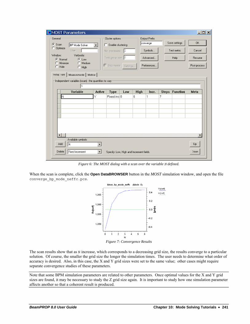
BeamPROP 8.0 User Guide Chapter 10: Mode Solving Tutorials • 241
Figure 6: The MOST dialog with a scan over the variable N defined.
When the scan is complete, click the Open DataBROWSER button in the MOST simulation window, and open the file converge_bp_mode_neffc.pcs.
Figure 7: Convergence Results
The scan results show that as N increase, which corresponds to a decreasing grid size, the results converge to a particular solution. Of course, the smaller the grid size the longer the simulation times. The user needs to determine what order of accuracy is desired. Also, in this case, the X and Y grid sizes were set to the same value; other cases might require separate convergence studies of these parameters.
Note that some BPM simulation parameters are related to other parameters. Once optimal values for the X and Y grid sizes are found, it may be necessary to study the Z grid size again. It is important to study how one simulation parameter affects another so that a coherent result is produced.
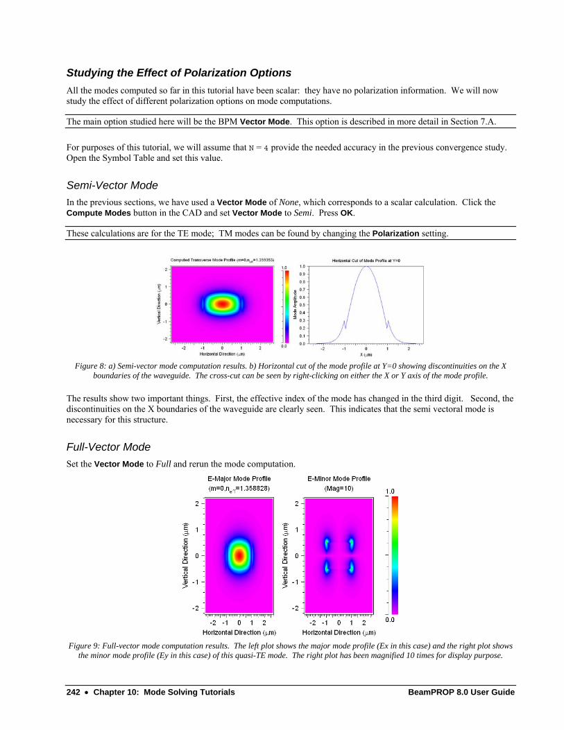
242 • Chapter 10: Mode Solving Tutorials BeamPROP 8.0 User Guide
Studying the Effect of Polarization Options All the modes computed so far in this tutorial have been scalar: they have no polarization information. We will now study the effect of different polarization options on mode computations.
The main option studied here will be the BPM Vector Mode. This option is described in more detail in Section 7.A.
For purposes of this tutorial, we will assume that N = 4 provide the needed accuracy in the previous convergence study. Open the Symbol Table and set this value.
Semi-Vector Mode In the previous sections, we have used a Vector Mode of None, which corresponds to a scalar calculation. Click the Compute Modes button in the CAD and set Vector Mode to Semi. Press OK.
These calculations are for the TE mode; TM modes can be found by changing the Polarization setting.
Figure 8: a) Semi-vector mode computation results. b) Horizontal cut of the mode profile at Y=0 showing discontinuities on the X
boundaries of the waveguide. The cross-cut can be seen by right-clicking on either the X or Y axis of the mode profile.
The results show two important things. First, the effective index of the mode has changed in the third digit. Second, the discontinuities on the X boundaries of the waveguide are clearly seen. This indicates that the semi vectoral mode is necessary for this structure.
Full-Vector Mode Set the Vector Mode to Full and rerun the mode computation.
Figure 9: Full-vector mode computation results. The left plot shows the major mode profile (Ex in this case) and the right plot shows
the minor mode profile (Ey in this case) of this quasi-TE mode. The right plot has been magnified 10 times for display purpose.

BeamPROP 8.0 User Guide Chapter 10: Mode Solving Tutorials • 243
The mode profile from the full-vector computation appears similar to the semi-vector results, except the effective index differs in the fourth or fifth digit. If this accuracy is necessary, then a full vector simulation is necessary. Otherwise, a semi-vector simulation, which is faster and sometimes more robust, is sufficient.
While not explored here, it is typically a good idea to again study the grid size after enabling polarization options to ensure that an accurate result is obtained.
Areas for Further Exploration • Convergence studies and Polarization in 2D
This tutorial performed convergence studies and explored polarization options in 3D only. Try performing similar studies in 2D
• Perform additional convergence studies
This tutorial did not perform a comprehensive convergence study for X, Y, and Z grid sizes and polarization options. Try these on your own and see how each option affects the other.

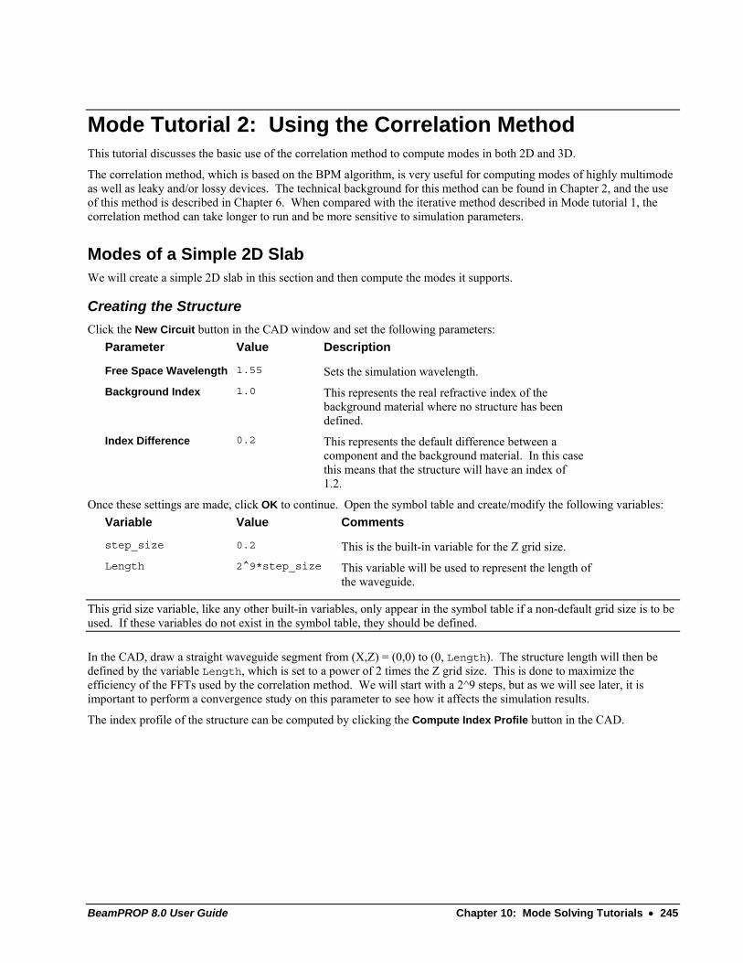
BeamPROP 8.0 User Guide Chapter 10: Mode Solving Tutorials • 245
Mode Tutorial 2: Using the Correlation Method This tutorial discusses the basic use of the correlation method to compute modes in both 2D and 3D.
The correlation method, which is based on the BPM algorithm, is very useful for computing modes of highly multimode as well as leaky and/or lossy devices. The technical background for this method can be found in Chapter 2, and the use of this method is described in Chapter 6. When compared with the iterative method described in Mode tutorial 1, the correlation method can take longer to run and be more sensitive to simulation parameters.
Modes of a Simple 2D Slab We will create a simple 2D slab in this section and then compute the modes it supports.
Creating the Structure Click the New Circuit button in the CAD window and set the following parameters: Parameter Value Description
Free Space Wavelength 1.55 Sets the simulation wavelength.
Background Index 1.0 This represents the real refractive index of the background material where no structure has been defined.
Index Difference 0.2 This represents the default difference between a component and the background material. In this case this means that the structure will have an index of 1.2.
Once these settings are made, click OK to continue. Open the symbol table and create/modify the following variables: Variable Value Comments
step_size 0.2 This is the built-in variable for the Z grid size.
Length 2^9*step_size This variable will be used to represent the length of the waveguide.
This grid size variable, like any other built-in variables, only appear in the symbol table if a non-default grid size is to be used. If these variables do not exist in the symbol table, they should be defined.
In the CAD, draw a straight waveguide segment from (X,Z) = (0,0) to (0, Length). The structure length will then be defined by the variable Length, which is set to a power of 2 times the Z grid size. This is done to maximize the efficiency of the FFTs used by the correlation method. We will start with a 2^9 steps, but as we will see later, it is important to perform a convergence study on this parameter to see how it affects the simulation results.
The index profile of the structure can be computed by clicking the Compute Index Profile button in the CAD.
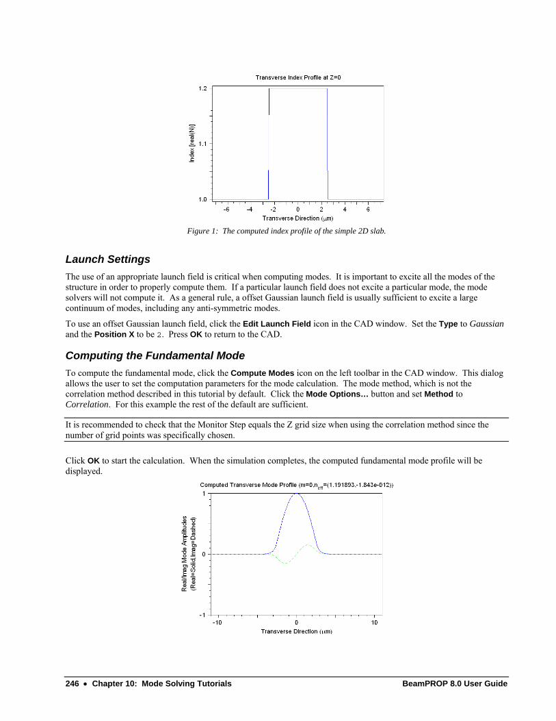
246 • Chapter 10: Mode Solving Tutorials BeamPROP 8.0 User Guide
Figure 1: The computed index profile of the simple 2D slab.
Launch Settings The use of an appropriate launch field is critical when computing modes. It is important to excite all the modes of the structure in order to properly compute them. If a particular launch field does not excite a particular mode, the mode solvers will not compute it. As a general rule, a offset Gaussian launch field is usually sufficient to excite a large continuum of modes, including any anti-symmetric modes.
To use an offset Gaussian launch field, click the Edit Launch Field icon in the CAD window. Set the Type to Gaussian and the Position X to be 2. Press OK to return to the CAD.
Computing the Fundamental Mode To compute the fundamental mode, click the Compute Modes icon on the left toolbar in the CAD window. This dialog allows the user to set the computation parameters for the mode calculation. The mode method, which is not the correlation method described in this tutorial by default. Click the Mode Options… button and set Method to Correlation. For this example the rest of the default are sufficient.
It is recommended to check that the Monitor Step equals the Z grid size when using the correlation method since the number of grid points was specifically chosen.
Click OK to start the calculation. When the simulation completes, the computed fundamental mode profile will be displayed.
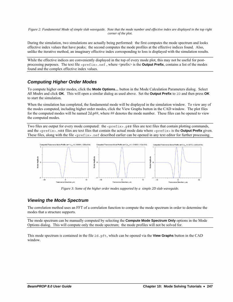
BeamPROP 8.0 User Guide Chapter 10: Mode Solving Tutorials • 247
Figure 2: Fundamental Mode of simple slab waveguide. Note that the mode number and effective index are displayed in the top right corner of the plot.
During the simulation, two simulations are actually being performed: the first computes the mode spectrum and looks effective index values that have peaks; the second computes the mode profiles at the effective indices found. Also, unlike the iterative method, an imaginary effective index corresponding to loss is displayed with the simulation results.
While the effective indices are conveniently displayed in the top of every mode plot, this may not be useful for post-processing purposes. The text file <prefix>.nef , where <prefix> is the Output Prefix, contains a list of the modes found and the complex effective index values.
Computing Higher Order Modes To compute higher order modes, click the Mode Options… button in the Mode Calculation Parameters dialog. Select All Modes and click OK. This will open a similar dialog as used above. Set the Output Prefix to 2D and then press OK to start the simulation.
When the simulation has completed, the fundamental mode will be displayed in the simulation window. To view any of the modes computed, including higher order modes, click the View Graphs button in the CAD window. The plot files for the computed modes will be named 2d.p##, where ## denotes the mode number. These files can be opened to view the computed modes.
Two files are output for every mode computed: the <prefix>.p## files are text files that contain plotting commands, and the <prefix>.m## files are text files that contain the actual mode data where <prefix> is the Output Prefix given. These files, along with the file <prefix>.nef described earlier can be opened in any text editor for further processing.
Figure 3: Some of the higher order modes supported by a simple 2D slab waveguide.
Viewing the Mode Spectrum The correlation method uses an FFT of a correlation function to compute the mode spectrum in order to determine the modes that a structure supports.
The mode spectrum can be manually computed by selecting the Compute Mode Spectrum Only options in the Mode Options dialog. This will compute only the mode spectrum; the mode profiles will not be solved for.
This mode spectrum is contained in the file 2d.pft, which can be opened via the View Graphs button in the CAD window.
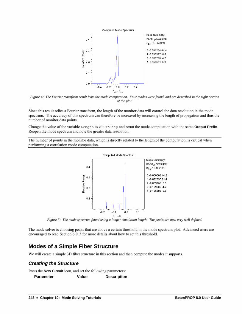
248 • Chapter 10: Mode Solving Tutorials BeamPROP 8.0 User Guide
Figure 4: The Fourier transform result from the mode computation. Four modes were found, and are described in the right portion
of the plot.
Since this result relies a Fourier transform, the length of the monitor data will control the data resolution in the mode spectrum. The accuracy of this spectrum can therefore be increased by increasing the length of propagation and thus the number of monitor data points.
Change the value of the variable Length to 2^13*Step and rerun the mode computation with the same Output Prefix. Reopen the mode spectrum and note the greater data resolution.
The number of points in the monitor data, which is directly related to the length of the computation, is critical when performing a correlation mode computation.
Figure 5: The mode spectrum found using a longer simulation length. The peaks are now very well defined.
The mode solver is choosing peaks that are above a certain threshold in the mode spectrum plot. Advanced users are encouraged to read Section 6.D.3 for more details about how to set this threshold.
Modes of a Simple Fiber Structure We will create a simple 3D fiber structure in this section and then compute the modes it supports.
Creating the Structure Press the New Circuit icon, and set the following parameters: Parameter Value Description
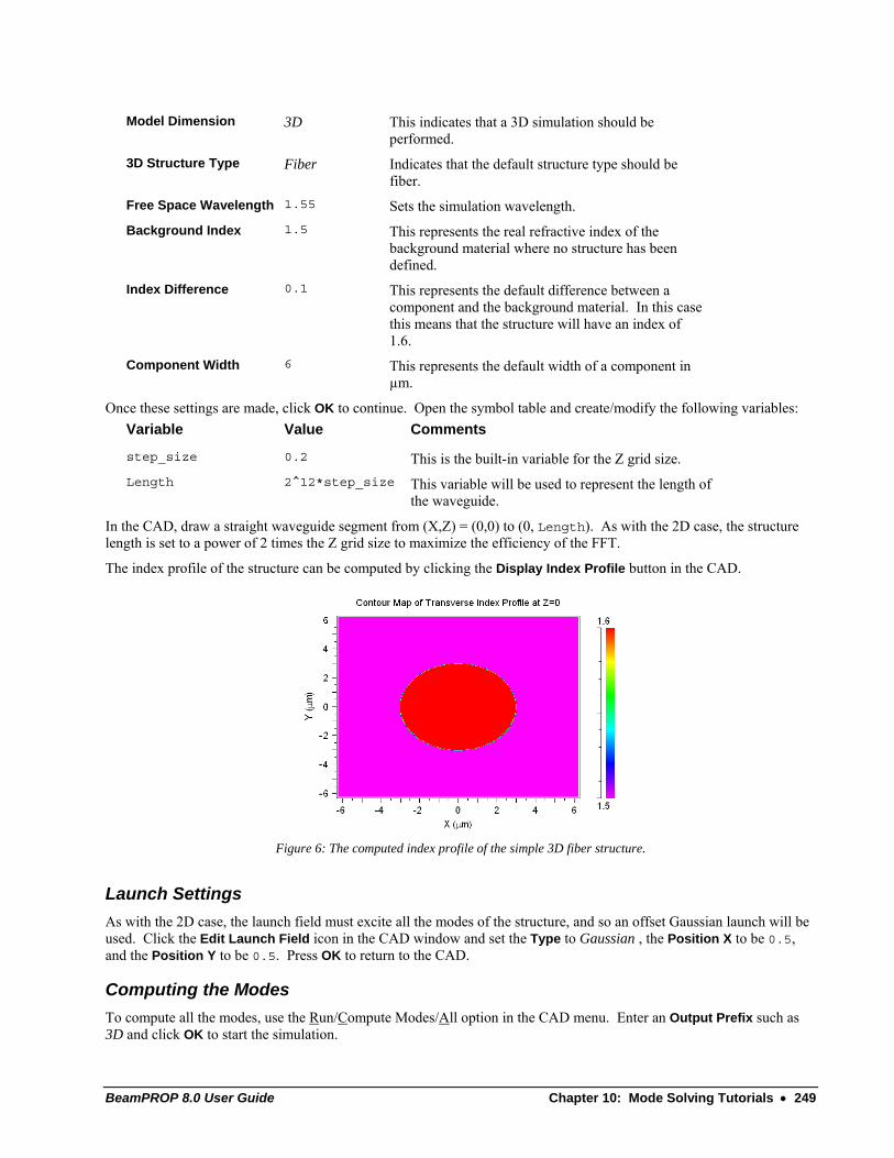
BeamPROP 8.0 User Guide Chapter 10: Mode Solving Tutorials • 249
Model Dimension 3D This indicates that a 3D simulation should be performed.
3D Structure Type Fiber Indicates that the default structure type should be fiber.
Free Space Wavelength 1.55 Sets the simulation wavelength.
Background Index 1.5 This represents the real refractive index of the background material where no structure has been defined.
Index Difference 0.1 This represents the default difference between a component and the background material. In this case this means that the structure will have an index of 1.6.
Component Width 6 This represents the default width of a component in µm.
Once these settings are made, click OK to continue. Open the symbol table and create/modify the following variables: Variable Value Comments
step_size 0.2 This is the built-in variable for the Z grid size.
Length 2^12*step_size This variable will be used to represent the length of the waveguide.
In the CAD, draw a straight waveguide segment from (X,Z) = (0,0) to (0, Length). As with the 2D case, the structure length is set to a power of 2 times the Z grid size to maximize the efficiency of the FFT.
The index profile of the structure can be computed by clicking the Display Index Profile button in the CAD.
Figure 6: The computed index profile of the simple 3D fiber structure.
Launch Settings As with the 2D case, the launch field must excite all the modes of the structure, and so an offset Gaussian launch will be used. Click the Edit Launch Field icon in the CAD window and set the Type to Gaussian , the Position X to be 0.5, and the Position Y to be 0.5. Press OK to return to the CAD.
Computing the Modes To compute all the modes, use the Run/Compute Modes/All option in the CAD menu. Enter an Output Prefix such as 3D and click OK to start the simulation.
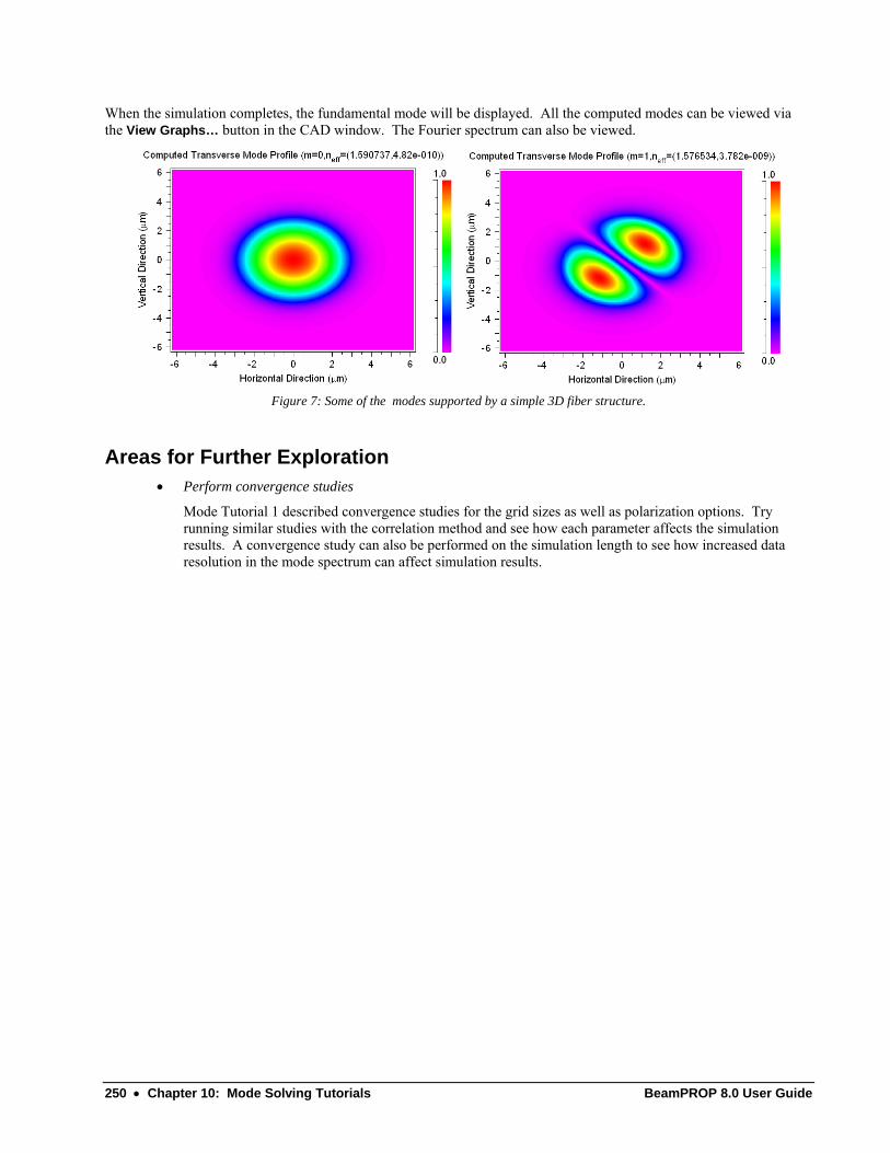
250 • Chapter 10: Mode Solving Tutorials BeamPROP 8.0 User Guide
When the simulation completes, the fundamental mode will be displayed. All the computed modes can be viewed via the View Graphs… button in the CAD window. The Fourier spectrum can also be viewed.
Figure 7: Some of the modes supported by a simple 3D fiber structure.
Areas for Further Exploration • Perform convergence studies
Mode Tutorial 1 described convergence studies for the grid sizes as well as polarization options. Try running similar studies with the correlation method and see how each parameter affects the simulation results. A convergence study can also be performed on the simulation length to see how increased data resolution in the mode spectrum can affect simulation results.

BeamPROP 8.0 User Guide Chapter 10: Mode Solving Tutorials • 251
Mode Tutorial 3: Computing the Mode Cutoff This tutorial illustrates the computation of the mode cutoff at which a structure becomes single-mode. This tutorial uses the correlation mode solving method, but the iterative method could be used as well.
The modes of a channel structure will be studied as the waveguide dimensions are changed. This type of analysis could also be done for any other parameter including wavelength and refractive index.
User familiarity with the correlation method is assumed. See Mode Tutorial 2 for more details on the correlation method.
Creating the Structure Press the New Circuit icon and set the following parameters: Parameter Value Description Model Dimension 3D Enables a 3D simulation. 3D Structure Type Channel Sets the default structure type to channel. Free Space Wavelength 1.55 Sets the simulation wavelength. Background Index 1.48 This represents the real refractive index of
the background material where no structure has been defined.
Index Difference 0.02 This represents the default difference between a component and the background material. In this case this means that the structure will have an index of 1.5.
Component Width 7 Sets the width of the channel segment.
Once these settings are made, click OK to continue. Open the symbol table and create/modify the following variables: Variable Value Description step_size 1 Sets the Z grid size. Length 2^10*step_size This variable will be used to set the length o
the segment. It’s value has been chose tn maximize the efficiency of the FFTs used by the correlation method.
This grid size variable, like any other built-in variables, only appear in the symbol table if a non-default grid size is to be used. If these variables do not exist in the symbol table, they should be defined.
In the CAD, draw a straight waveguide segment from (X,Z) = (0,0) to (0, Length). The structure length will then be defined by the variable Length.
Setting Simulation Parameters This tutorial will use the correlation method. To enable this method, click the Compute Modes button I the left toolbar and then click the Mode Options… button. Set Method to Correlation and press OK twice to return to the CAD.
To set the launch parameters, click the Edit Launch Field button on the CAD toolbar and set the following parameters: Parameter Value Description
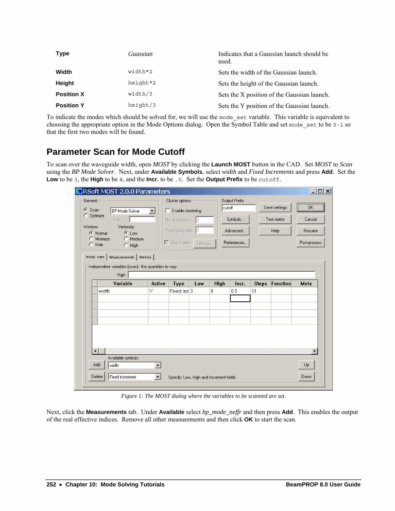
252 • Chapter 10: Mode Solving Tutorials BeamPROP 8.0 User Guide
Type Guassian Indicates that a Gaussian launch should be used.
Width width*2 Sets the width of the Gaussian launch. Height height*2 Sets the height of the Gaussian launch. Position X width/3 Sets the X position of the Gaussian launch. Position Y height/3 Sets the Y position of the Gaussian launch.
To indicate the modes which should be solved for, we will use the mode_set variable. This variable is equivalent to choosing the appropriate option in the Mode Options dialog. Open the Symbol Table and set mode_set to be 0-1 so that the first two modes will be found.
Parameter Scan for Mode Cutoff To scan over the waveguide width, open MOST by clicking the Launch MOST button in the CAD. Set MOST to Scan using the BP Mode Solver. Next, under Available Symbols, select width and Fixed Increments and press Add. Set the Low to be 3, the High to be 8, and the Incr. to be .5. Set the Output Prefix to be cutoff.
Figure 1: The MOST dialog where the variables to be scanned are set.
Next, click the Measurements tab. Under Available select bp_mode_neffr and then press Add. This enables the output of the real effective indices. Remove all other measurements and then click OK to start the scan.
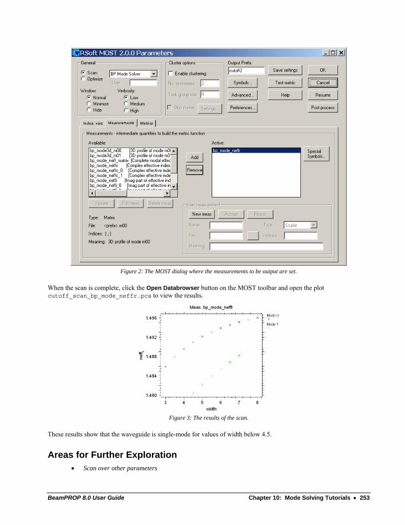
BeamPROP 8.0 User Guide Chapter 10: Mode Solving Tutorials • 253
Figure 2: The MOST dialog where the measurements to be output are set.
When the scan is complete, click the Open Databrowser button on the MOST toolbar and open the plot cutoff_scan_bp_mode_neffr.pcs to view the results.
Figure 3: The results of the scan.
These results show that the waveguide is single-mode for values of width below 4.5.
Areas for Further Exploration • Scan over other parameters

254 • Chapter 10: Mode Solving Tutorials BeamPROP 8.0 User Guide
This example scanned over the waveguide dimensions. Try scanning over other parameters such as the wavelength or refractive index.
• Determine the cutoff point more accurately
This scan used a coarse step of 0.5. Try rerunning the scan to find the cutoff point more accurately.
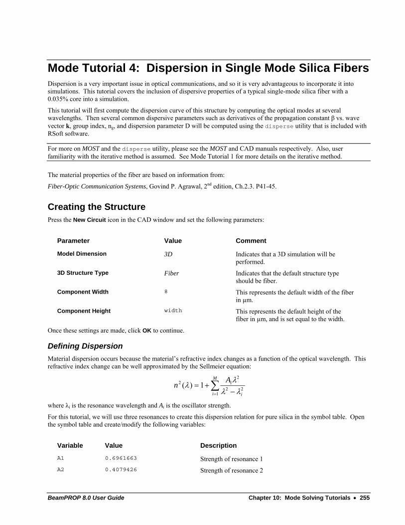
BeamPROP 8.0 User Guide Chapter 10: Mode Solving Tutorials • 255
Mode Tutorial 4: Dispersion in Single Mode Silica Fibers Dispersion is a very important issue in optical communications, and so it is very advantageous to incorporate it into simulations. This tutorial covers the inclusion of dispersive properties of a typical single-mode silica fiber with a 0.035% core into a simulation.
This tutorial will first compute the dispersion curve of this structure by computing the optical modes at several wavelengths. Then several common dispersive parameters such as derivatives of the propagation constant β vs. wave vector k, group index, ng, and dispersion parameter D will be computed using the disperse utility that is included with RSoft software.
For more on MOST and the disperse utility, please see the MOST and CAD manuals respectively. Also, user familiarity with the iterative method is assumed. See Mode Tutorial 1 for more details on the iterative method.
The material properties of the fiber are based on information from:
Fiber-Optic Communication Systems, Govind P. Agrawal, 2nd edition, Ch.2.3. P41-45.
Creating the Structure Press the New Circuit icon in the CAD window and set the following parameters:
Parameter Value Comment Model Dimension 3D Indicates that a 3D simulation will be
performed. 3D Structure Type Fiber Indicates that the default structure type
should be fiber. Component Width 8 This represents the default width of the fiber
in µm. Component Height width This represents the default height of the
fiber in µm, and is set equal to the width.
Once these settings are made, click OK to continue.
Defining Dispersion Material dispersion occurs because the material’s refractive index changes as a function of the optical wavelength. This refractive index change can be well approximated by the Sellmeier equation:
∑= −
+=M
i i
iAn
122
22 1)(
λλλ
λ
where λi is the resonance wavelength and Ai is the oscillator strength.
For this tutorial, we will use three resonances to create this dispersion relation for pure silica in the symbol table. Open the symbol table and create/modify the following variables:
Variable Value Description A1 0.6961663 Strength of resonance 1 A2 0.4079426 Strength of resonance 2
256 • Chapter 10: Mode Solving Tutorials BeamPROP 8.0 User Guide
A3 0.8974794 Strength of resonance 3 L1 0.0684043 Location of resonance 1 (in µm) L2 0.1162414 Location of resonance 2 (in µm) L3 9.896161 Location of resonance 3 (in µm) L free_space_wavelength The built-in variable free_space_wavelength
defines the simulation wavelength. This definition defines the variable L as a convenient way to reference this wavelength.
R1 A1*L^2/(L^2-L1^2) Resonance 1 R2 A2*L^2/(L^2-L2^2) Resonance 2 R3 A3*L^2/(L^2-L3^2) Resonance 3
Once these parameters have been defined, we can define the index of the fiber. For this fiber, we will define the cladding index equal to the equation given above, and the index of the core will be 0.035% higher. Modify the following variables in the symbol table:
Variable Value Description background_index sqrt(1+R1+R2+R3) Sets the index of the fiber cladding. Note
that in this example, we are only considering the core/cladding interface, which is generally a very good approximation since the modes are well-guided.
delta .035*background_index Sets the core index as a function of the cladding index.
The definition of the material index (background_index, delta) is now logically tied to the simulation wavelength (free_space_wavelength): when the value of the wavelength is changed, the index values will change according to the equation above.
While in this case we used an equation to define the material dispersion, the user can also use data files or the Material Editor to define material dispersion. See Section 5.G.3. of the CAD manual for more details.
Once these variables have been defined, click OK to return to the CAD.
Creating the Fiber In the CAD, draw in a straight segment from (X,Z)= (0,0) to (0, 1000). The structure length, in this case 1000 µm, need only be long enough to allow the iterative mode solver to converge.
Computing Dispersion with MOST Once the fiber has been created so that its refractive index is a function of wavelength, we can use MOST to scan over the wavelength and compute the fiber mode. MOST can also be used to perform post-processing with the disperse utility to compute several common dispersion parameters.
Click the MOST button in the CAD toolbar to open the MOST dialog.
Creating the Parameter Scan We are going to compute the mode of the fiber over a wavelength range of 1.1 µm to 1.8 µm with an increment of 0.01. Create a scan with these parameters in the MOST dialog, including an Output Prefix of fiber.
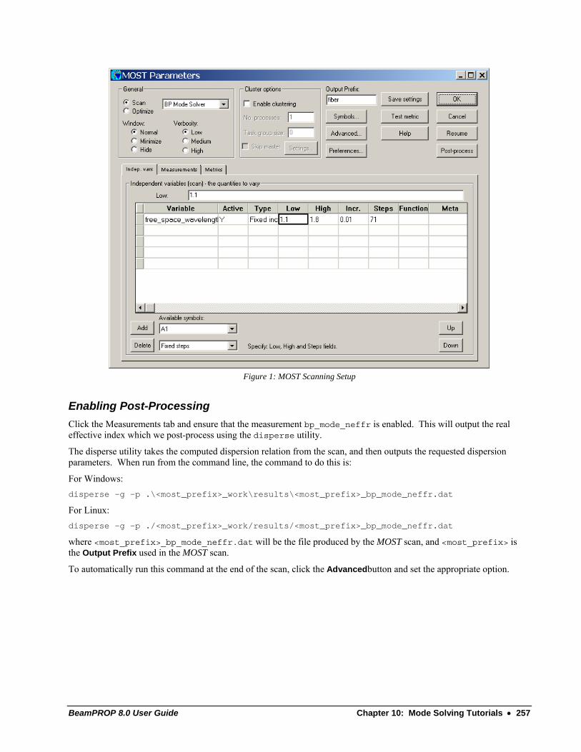
BeamPROP 8.0 User Guide Chapter 10: Mode Solving Tutorials • 257
Figure 1: MOST Scanning Setup
Enabling Post-Processing Click the Measurements tab and ensure that the measurement bp_mode_neffr is enabled. This will output the real effective index which we post-process using the disperse utility.
The disperse utility takes the computed dispersion relation from the scan, and then outputs the requested dispersion parameters. When run from the command line, the command to do this is:
For Windows: disperse –g –p .\<most_prefix>_work\results\<most_prefix>_bp_mode_neffr.dat
For Linux: disperse –g –p ./<most_prefix>_work/results/<most_prefix>_bp_mode_neffr.dat
where <most_prefix>_bp_mode_neffr.dat will be the file produced by the MOST scan, and <most_prefix> is the Output Prefix used in the MOST scan.
To automatically run this command at the end of the scan, click the Advancedbutton and set the appropriate option.
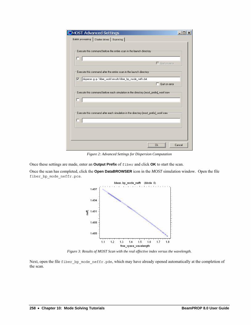
258 • Chapter 10: Mode Solving Tutorials BeamPROP 8.0 User Guide
Figure 2: Advanced Settings for Dispersion Computation
Once these settings are made, enter an Output Prefix of fiber and click OK to start the scan.
Once the scan has completed, click the Open DataBROWSER icon in the MOST simulation window. Open the file fiber_bp_mode_neffr.pcs.
Figure 3: Results of MOST Scan with the real effective index versus the wavelength.
Next, open the file fiber_bp_mode_neffr.pde, which may have already opened automatically at the completion of the scan.
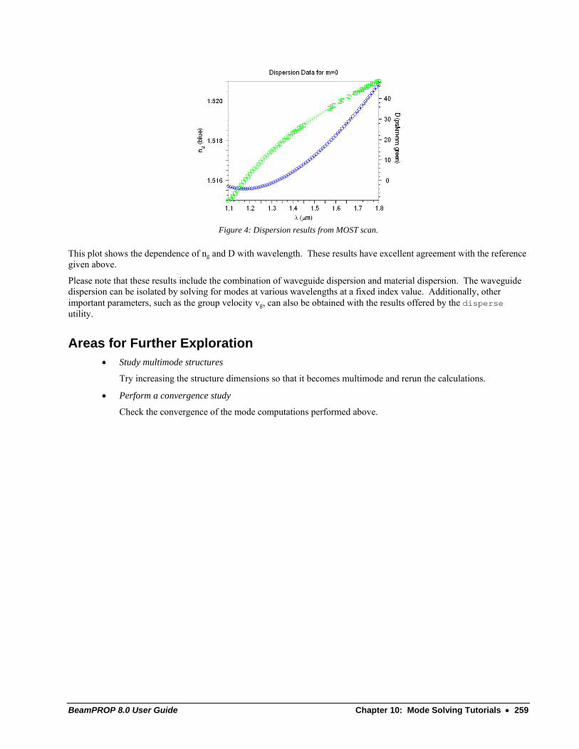
BeamPROP 8.0 User Guide Chapter 10: Mode Solving Tutorials • 259
Figure 4: Dispersion results from MOST scan.
This plot shows the dependence of ng and D with wavelength. These results have excellent agreement with the reference given above.
Please note that these results include the combination of waveguide dispersion and material dispersion. The waveguide dispersion can be isolated by solving for modes at various wavelengths at a fixed index value. Additionally, other important parameters, such as the group velocity vg, can also be obtained with the results offered by the disperse utility.
Areas for Further Exploration • Study multimode structures
Try increasing the structure dimensions so that it becomes multimode and rerun the calculations.
• Perform a convergence study
Check the convergence of the mode computations performed above.

BeamPROP 8.0 User Guide Chapter 10: Mode Solving Tutorials • 261
Mode Tutorial 5: Index Guided Photonic Crystal Fibers Photonic crystal fibers (PCFs) rely on various repeated defects in order to confine light in a core. The BPM mode solvers have the capability of solving for the modes of index guided PCFs since the confinement is due to Bragg reflection effects. Air guided PCFs, however, must be solved by other tools, such as RSoft’s FemSIM and BandSOLVE packages.
In this tutorial, we will solve for the modes of a PCF at different ratios of the period to wavelength. We will then determine ratios at which the fiber is single-moded for all wavelengths. It is based on:
T.A. Birks, J.C. Knight, and P. St. J. Russell, “Endlessly single-mode photonic crystal fiber,” Optics Letters, 22, 961 (1997)
This tutorial uses the iterative method. However, when looking to compute the modes of lossy PCFs, the correlation method should be used. User familiarity with the iterative method is assumed. See Mode Tutorial 1 for more details on the iterative method.
Creating the PCF Structure The creation of periodic arrays is greatly simplified through the use of the Array Layout Utility. Choose Utility/Array Layout from the CAD menu and set the following parameters:
Parameter Value Comment
Dimensions 2D (XY) This indicates that a 2D array should be created. In this array, the objects will represent air holes.
Lattice type Hexagonal Rings This indicates that a hexagonal ring lattice should be used.
L 0
M 4
Contents Ellipse Indicates that a elliptical object should be used in each unit cell. These objects will represent air holes.
Output Prefix pcf The name of the .ind file to be created by the utility.
Click OK to close the utility and open the new design file. Open the symbol table and create/modify the following variables:
Variable Value Comment Q 1 This variable will be used to easily
scan logarithmically over the wavelength.
R 0.3 This variable will be used to set the ratio of the Period to hole diameter.
Period 2.3 width R*Period Sets the diameter of the air holes. height width free_space_wavelength Period/(10^Q) The simulation wavelength. The
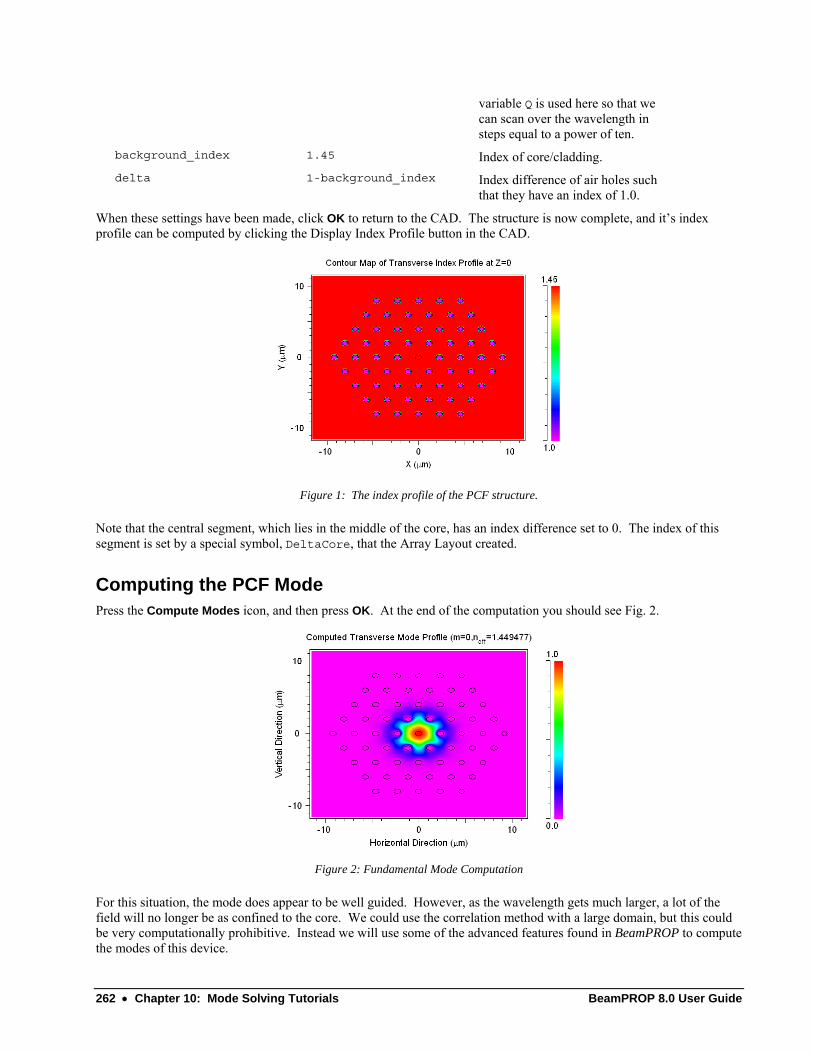
262 • Chapter 10: Mode Solving Tutorials BeamPROP 8.0 User Guide
variable Q is used here so that we can scan over the wavelength in steps equal to a power of ten.
background_index 1.45 Index of core/cladding. delta 1-background_index Index difference of air holes such
that they have an index of 1.0.
When these settings have been made, click OK to return to the CAD. The structure is now complete, and it’s index profile can be computed by clicking the Display Index Profile button in the CAD.
Figure 1: The index profile of the PCF structure.
Note that the central segment, which lies in the middle of the core, has an index difference set to 0. The index of this segment is set by a special symbol, DeltaCore, that the Array Layout created.
Computing the PCF Mode Press the Compute Modes icon, and then press OK. At the end of the computation you should see Fig. 2.
Figure 2: Fundamental Mode Computation
For this situation, the mode does appear to be well guided. However, as the wavelength gets much larger, a lot of the field will no longer be as confined to the core. We could use the correlation method with a large domain, but this could be very computationally prohibitive. Instead we will use some of the advanced features found in BeamPROP to compute the modes of this device.
BeamPROP 8.0 User Guide Chapter 10: Mode Solving Tutorials • 263
Exploring the Single-Mode Condition In order to explore the single-mode condition, we need to solve for the fundamental mode over a wide range of wavelengths. In a conventional fiber, the number of bound modes is governed by the V number, which increases without limit as the wavelength decreases. The reference above shows that it is possible to define an effective V number for a PCF that indicates reasonably accurately whether or not a fiber is single-moded:
2 22eff o effV n nπλΛ
= −
where Λ is the lattice period (Period), n0 is the glass index and neff is an “effective cladding index.” The effective cladding index can be considered as the effective index of the first radiation state, which is equivalent to finding the lowest mode in the band structure of the plain lattice. The reference shows that in contrast to step-index fibers, the Veff for a PCF converges to a finite value as the wavelength decreases. If the finite value is less than approximately 2.405, the PCF is single-moded.
Setting Simulation Parameters In order to compute the parameter neff in the above equation, we will solve for the mode of the plain lattice with no defect. This can be done by choosing boundary positions such that only a single unit cell lies within the domain, the use of symmetric boundary conditions, and a plane wave launch.
To do this, we will set all the simulation parameters via the symbol table. Open the symbol table and create/modify the following variables:
Variable Value Description boundary_min -Period/2 Sets the minimum X boundary location. boundary_max Period/2 Sets the maximum X boundary location. boundary_min_y -PeriodY Sets the minimum Y boundary location. boundary_max_y PeriodY Sets the maximum Y boundary location. bc_type_bottom BC_SYMMETRIC Sets the X minimum boundary type to symmetric. bc_type_top BC_SYMMETRIC Sets the X maximum boundary type to
symmetric. bc_type_left BC_SYMMETRIC Sets the Y minimum boundary type to symmetric. bc_type_right BC_SYMMETRIC Sets the Y maximum boundary type to
symmetric. DeltaCore delta The variable created by the Array Layout to set
the index of the central air hole. This value enables the presence of the central air hole.
grid_size width/16 Sets the grid size in X direction grid_size_y width/16 Sets the grid size in Y direction launch_type LAUNCH_RECTANGLE Enables a rectangular launch which will be used
to represent a plane wave. launch_width inf Launch size to excite mode. launch_height inf Launch size to excite mode. step_size_idbpm 0.005 Sets the grid size in the Z direction for the
iterative method. neff_tol 1e-009 Sets the Neff Tolerance used by the iterative
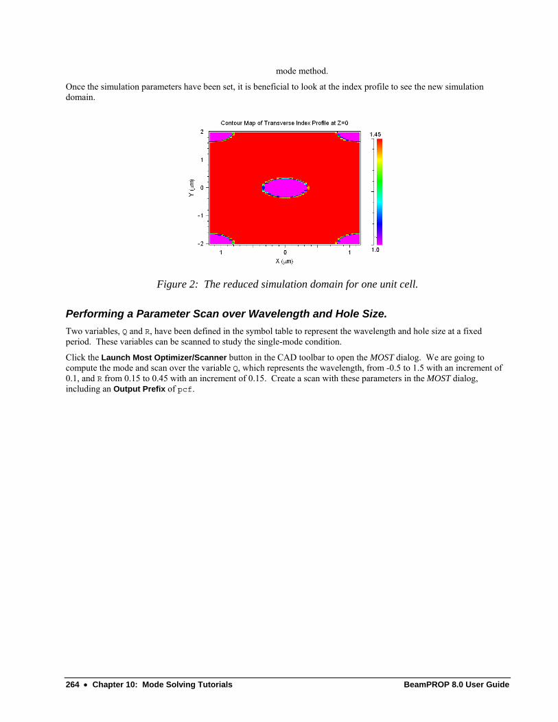
264 • Chapter 10: Mode Solving Tutorials BeamPROP 8.0 User Guide
mode method.
Once the simulation parameters have been set, it is beneficial to look at the index profile to see the new simulation domain.
Figure 2: The reduced simulation domain for one unit cell.
Performing a Parameter Scan over Wavelength and Hole Size. Two variables, Q and R, have been defined in the symbol table to represent the wavelength and hole size at a fixed period. These variables can be scanned to study the single-mode condition.
Click the Launch Most Optimizer/Scanner button in the CAD toolbar to open the MOST dialog. We are going to compute the mode and scan over the variable Q, which represents the wavelength, from -0.5 to 1.5 with an increment of 0.1, and R from 0.15 to 0.45 with an increment of 0.15. Create a scan with these parameters in the MOST dialog, including an Output Prefix of pcf.
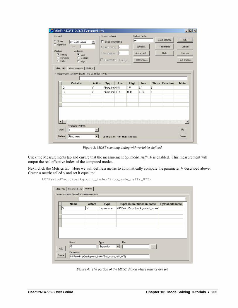
BeamPROP 8.0 User Guide Chapter 10: Mode Solving Tutorials • 265
Figure 3: MOST scanning dialog with variables defined.
Click the Measurements tab and ensure that the measurement bp_mode_neffr_0 is enabled. This measurement will output the real effective index of the computed modes.
Next, click the Metrics tab. Here we will define a metric to automatically compute the parameter V described above. Create a metric called V and set it equal to:
k0*Period*sqrt(background_index^2-bp_mode_neffr_0^2)
Figure 4: The portion of the MOST dialog where metrics are set.
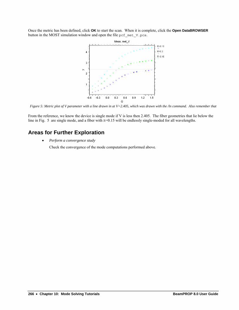
266 • Chapter 10: Mode Solving Tutorials BeamPROP 8.0 User Guide
Once the metric has been defined, click OK to start the scan. When it is complete, click the Open DataBROWSER button in the MOST simulation window and open the file pcf_met_V.pcs.
Figure 5: Metric plot of V parameter with a line drawn in at V=2.405, which was drawn with the /ln command. Also remember that
From the reference, we know the device is single mode if V is less then 2.405. The fiber geometries that lie below the line in Fig. 5 are single mode, and a fiber with R=0.15 will be endlessly single-moded for all wavelengths.
Areas for Further Exploration • Perform a convergence study
Check the convergence of the mode computations performed above.
BeamPROP 8.0 User Guide Chapter 10: Mode Solving Tutorials • 267
Mode Tutorial 6: Leaky Modes of a Rib Waveguide The iterative mode computation method, while it is very useful for fast mode computations of well-defined modes, it is not capable of finding lossy or leaky modes. This tutorial illustrates the use of the correlation method to solve for the leaky modes of a high index contrast rib waveguide with a thin silica buffer layer between the core and substrate.
User familiarity with the correlation method is assumed. See Mode Tutorial 2 for more details on the correlation method.
Creating the Structure Click the New Circuit button in the CAD toolbar, and set the following parameters:
Parameter Value Comment
Model Dimensions 3D This indicates that a 3D structure will be created.
3D Structure Type Multilayer Indicates that the default structure type should be multilayer.
Free Space Wavelength 1.55 Sets the simulation wavelength.
Background Index 3.5 For the case of a multilayer structure type, this sets the substrate index.
Index Difference 0.45
Component Width 5 This sets the width of a waveguide segment.
Component Height 1.75 This sets the height of a waveguide segment.
Cover Index 1.0 This sets the cover index.
Slab Height 1.0 This sets the height of the slab around the waveguide.
For more information about how a multilayer structure is defined, please see the CAD manual.
Next, press the Edit Layers… button and modify Layer Table 0 as follows:
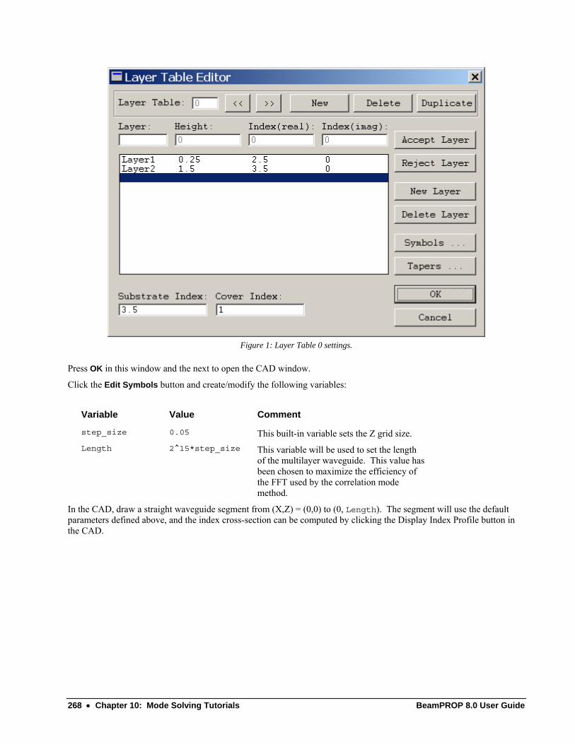
268 • Chapter 10: Mode Solving Tutorials BeamPROP 8.0 User Guide
Figure 1: Layer Table 0 settings.
Press OK in this window and the next to open the CAD window.
Click the Edit Symbols button and create/modify the following variables:
Variable Value Comment
step_size 0.05 This built-in variable sets the Z grid size.
Length 2^15*step_size This variable will be used to set the length of the multilayer waveguide. This value has been chosen to maximize the efficiency of the FFT used by the correlation mode method.
In the CAD, draw a straight waveguide segment from (X,Z) = (0,0) to (0, Length). The segment will use the default parameters defined above, and the index cross-section can be computed by clicking the Display Index Profile button in the CAD.
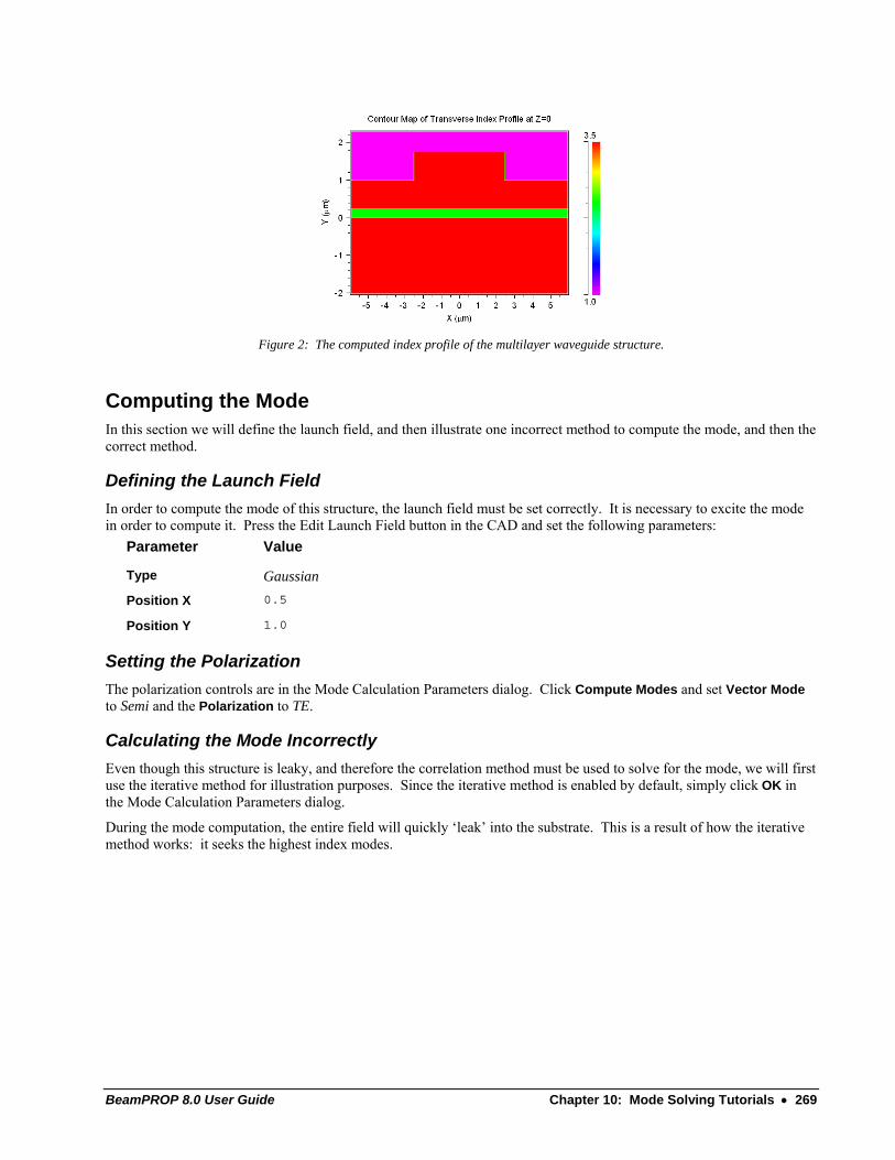
BeamPROP 8.0 User Guide Chapter 10: Mode Solving Tutorials • 269
Figure 2: The computed index profile of the multilayer waveguide structure.
Computing the Mode In this section we will define the launch field, and then illustrate one incorrect method to compute the mode, and then the correct method.
Defining the Launch Field In order to compute the mode of this structure, the launch field must be set correctly. It is necessary to excite the mode in order to compute it. Press the Edit Launch Field button in the CAD and set the following parameters: Parameter Value
Type Gaussian
Position X 0.5
Position Y 1.0
Setting the Polarization The polarization controls are in the Mode Calculation Parameters dialog. Click Compute Modes and set Vector Mode to Semi and the Polarization to TE.
Calculating the Mode Incorrectly Even though this structure is leaky, and therefore the correlation method must be used to solve for the mode, we will first use the iterative method for illustration purposes. Since the iterative method is enabled by default, simply click OK in the Mode Calculation Parameters dialog.
During the mode computation, the entire field will quickly ‘leak’ into the substrate. This is a result of how the iterative method works: it seeks the highest index modes.
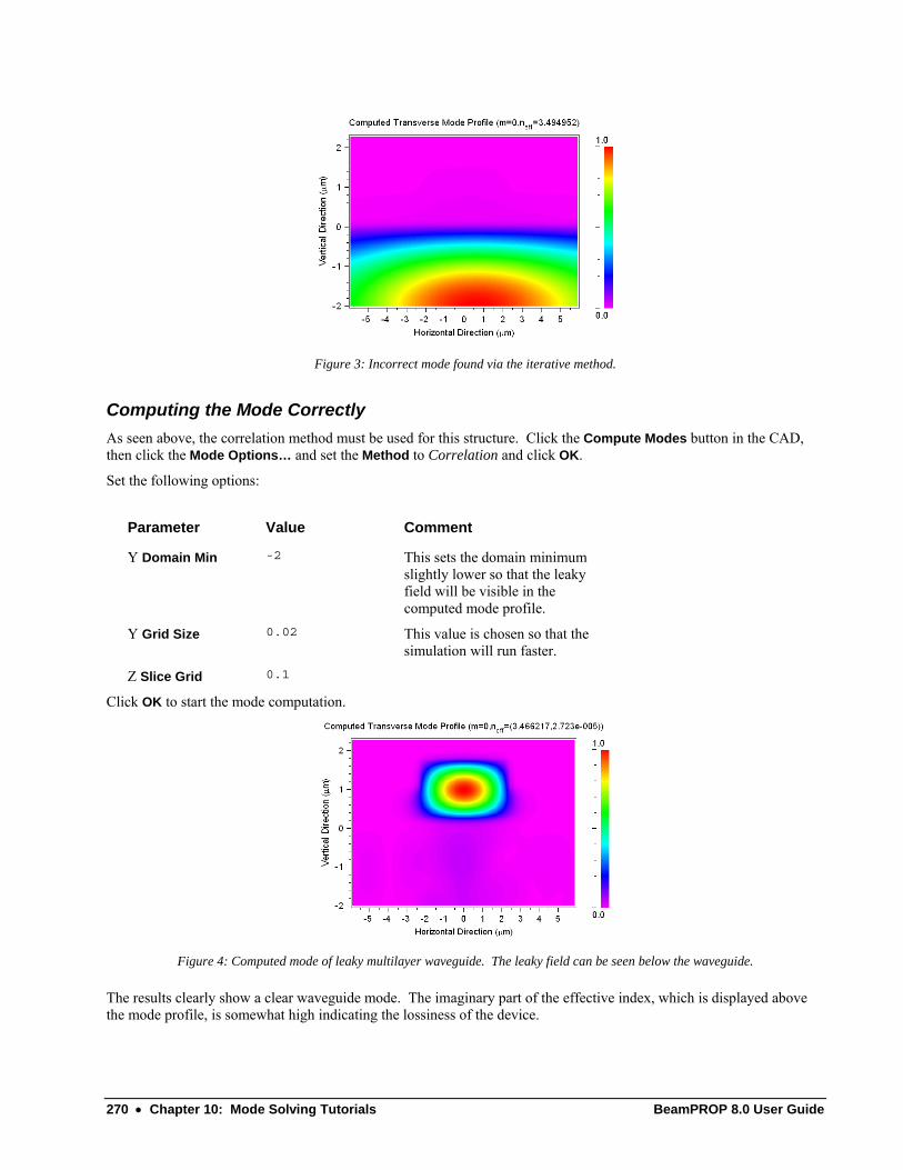
270 • Chapter 10: Mode Solving Tutorials BeamPROP 8.0 User Guide
Figure 3: Incorrect mode found via the iterative method.
Computing the Mode Correctly As seen above, the correlation method must be used for this structure. Click the Compute Modes button in the CAD, then click the Mode Options… and set the Method to Correlation and click OK.
Set the following options:
Parameter Value Comment
Y Domain Min -2 This sets the domain minimum slightly lower so that the leaky field will be visible in the computed mode profile.
Y Grid Size 0.02 This value is chosen so that the simulation will run faster.
Z Slice Grid 0.1
Click OK to start the mode computation.
Figure 4: Computed mode of leaky multilayer waveguide. The leaky field can be seen below the waveguide.
The results clearly show a clear waveguide mode. The imaginary part of the effective index, which is displayed above the mode profile, is somewhat high indicating the lossiness of the device.

BeamPROP 8.0 User Guide Chapter 10: Mode Solving Tutorials • 271
Areas for Further Exploration • Perform a convergence study
The example in this tutorial was run with slightly coarse simulation parameters in order to speed up the simulations. Try refining the parameters via a convergence study and see if the results change.

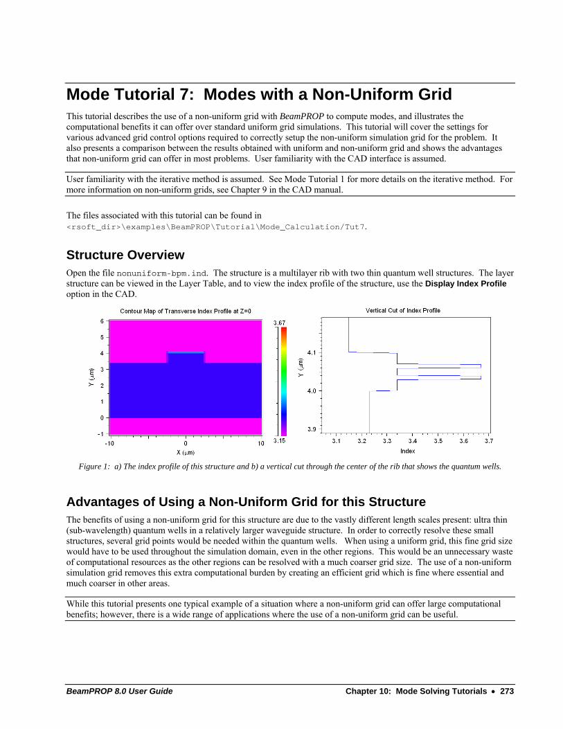
BeamPROP 8.0 User Guide Chapter 10: Mode Solving Tutorials • 273
Mode Tutorial 7: Modes with a Non-Uniform Grid This tutorial describes the use of a non-uniform grid with BeamPROP to compute modes, and illustrates the computational benefits it can offer over standard uniform grid simulations. This tutorial will cover the settings for various advanced grid control options required to correctly setup the non-uniform simulation grid for the problem. It also presents a comparison between the results obtained with uniform and non-uniform grid and shows the advantages that non-uniform grid can offer in most problems. User familiarity with the CAD interface is assumed.
User familiarity with the iterative method is assumed. See Mode Tutorial 1 for more details on the iterative method. For more information on non-uniform grids, see Chapter 9 in the CAD manual.
The files associated with this tutorial can be found in <rsoft_dir>\examples\BeamPROP\Tutorial\Mode_Calculation/Tut7.
Structure Overview Open the file nonuniform-bpm.ind. The structure is a multilayer rib with two thin quantum well structures. The layer structure can be viewed in the Layer Table, and to view the index profile of the structure, use the Display Index Profile option in the CAD.
Figure 1: a) The index profile of this structure and b) a vertical cut through the center of the rib that shows the quantum wells.
Advantages of Using a Non-Uniform Grid for this Structure The benefits of using a non-uniform grid for this structure are due to the vastly different length scales present: ultra thin (sub-wavelength) quantum wells in a relatively larger waveguide structure. In order to correctly resolve these small structures, several grid points would be needed within the quantum wells. When using a uniform grid, this fine grid size would have to be used throughout the simulation domain, even in the other regions. This would be an unnecessary waste of computational resources as the other regions can be resolved with a much coarser grid size. The use of a non-uniform simulation grid removes this extra computational burden by creating an efficient grid which is fine where essential and much coarser in other areas.
While this tutorial presents one typical example of a situation where a non-uniform grid can offer large computational benefits; however, there is a wide range of applications where the use of a non-uniform grid can be useful.
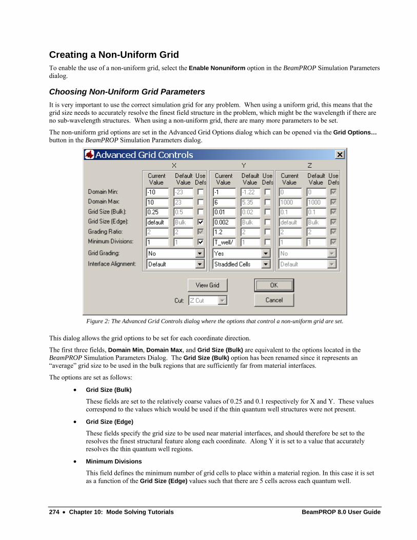
274 • Chapter 10: Mode Solving Tutorials BeamPROP 8.0 User Guide
Creating a Non-Uniform Grid To enable the use of a non-uniform grid, select the Enable Nonuniform option in the BeamPROP Simulation Parameters dialog.
Choosing Non-Uniform Grid Parameters It is very important to use the correct simulation grid for any problem. When using a uniform grid, this means that the grid size needs to accurately resolve the finest field structure in the problem, which might be the wavelength if there are no sub-wavelength structures. When using a non-uniform grid, there are many more parameters to be set.
The non-uniform grid options are set in the Advanced Grid Options dialog which can be opened via the Grid Options… button in the BeamPROP Simulation Parameters dialog.
Figure 2: The Advanced Grid Controls dialog where the options that control a non-uniform grid are set.
This dialog allows the grid options to be set for each coordinate direction.
The first three fields, Domain Min, Domain Max, and Grid Size (Bulk) are equivalent to the options located in the BeamPROP Simulation Parameters Dialog. The Grid Size (Bulk) option has been renamed since it represents an “average” grid size to be used in the bulk regions that are sufficiently far from material interfaces.
The options are set as follows:
• Grid Size (Bulk)
These fields are set to the relatively coarse values of 0.25 and 0.1 respectively for X and Y. These values correspond to the values which would be used if the thin quantum well structures were not present.
• Grid Size (Edge)
These fields specify the grid size to be used near material interfaces, and should therefore be set to the resolves the finest structural feature along each coordinate. Along Y it is set to a value that accurately resolves the thin quantum well regions.
• Minimum Divisions
This field defines the minimum number of grid cells to place within a material region. In this case it is set as a function of the Grid Size (Edge) values such that there are 5 cells across each quantum well.
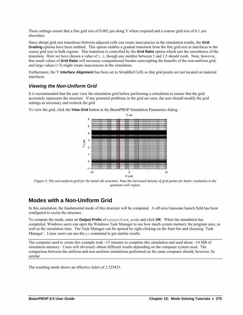
BeamPROP 8.0 User Guide Chapter 10: Mode Solving Tutorials • 275
These settings ensure that a fine grid size of 0.002 μm along Y where required and a coarser grid size of 0.1 μm elsewhere.
Since abrupt grid size transitions between adjacent cells can create inaccuracies in the simulation results, the Grid Grading options have been enabled. This option enables a gradual transition from the fine grid size at interfaces to the coarse grid size in bulk regions. This transition is controlled by the Grid Ratio option which sets the smoothness of the transition. Here we have chosen a value of 1.2, though any number between 1 and 1.5 should work. Note, however, that small values of Grid Ratio will increases computational burden outweighing the benefits of the non-uniform grid, and large values (>2) might create inaccuracies in the simulation.
Furthermore, the Y Interface Alignment has been set to Straddled Cells so that grid points are not located on material interfaces.
Viewing the Non-Uniform Grid It is recommended that the user view the simulation grid before performing a simulation to ensure that the grid accurately represents the structure. If any potential problems in the grid are seen, the user should modify the grid settings as necessary and recheck the grid.
To view the grid, click the View Grid button in the BeamPROP Simulation Parameters dialog.
Figure 3: The non-uniform grid for the metal slit structure. Note the increased density of grid points for better resolution in the
quantum well region.
Modes with a Non-Uniform Grid In this simulation, the fundamental mode of this structure will be computed. A off-axis Gaussian launch field has been configured to excite the structure.
To compute the mode, enter an Output Prefix of nonuniform_mode and click OK. When the simulation has completed, Windows users can open the Windows Task Manager to see how much system memory the program uses, as well as the simulation time. The Task Manager can be opened by right-clicking on the Start bar and choosing ‘Task Manager’. Linux users can use the ps command to get similar results.
The computer used to create this example took ~15 minutes to complete this simulation and used about ~14 MB of simulation memory. Users will obviously obtain different results depending on the computer system used. The comparison between the uniform and non-uniform simulations performed on the same computer should, however, be similar.
The resulting mode shows an effective index of 3.225423.
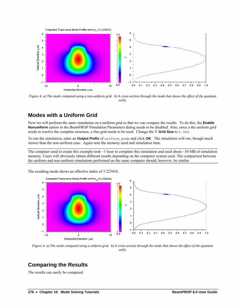
276 • Chapter 10: Mode Solving Tutorials BeamPROP 8.0 User Guide
Figure 4: a) The mode computed using a non-uniform grid. b) A cross-section through the mode that shows the effect of the quantum
wells.
Modes with a Uniform Grid Next we will perform the same simulation on a uniform grid so that we can compare the results. To do this, the Enable Nonuniform option in the BeamPROP Simulation Parameters dialog needs to be disabled. Also, since a the uniform grid needs to resolve the complete structure, a fine grid needs to be used. Change the Y Grid Size to 0.002.
To run the simulation, enter an Output Prefix of uniform_mode and click OK. The simulation will run, though much slower than the non-uniform case. Again note the memory used and simulation time.
The computer used to create this example took ~1 hour to complete this simulation and used about ~30 MB of simulation memory. Users will obviously obtain different results depending on the computer system used. The comparison between the uniform and non-uniform simulations performed on the same computer should, however, be similar.
The resulting mode shows an effective index of 3.225434.
Figure 4: a) The mode computed using a uniform grid. b) A cross-section through the mode that shows the effect of the quantum
wells.
Comparing the Results The results can easily be compared:

BeamPROP 8.0 User Guide Chapter 10: Mode Solving Tutorials • 277
• Total Simulation Time:
The use of a non-uniform grid decreased the total simulation time from about 60 minutes to 15 minutes, resulting in a simulation that is about 4 times faster. Remember that results may vary depending on the computer system used. but a similar speedup should be seen.
• Required Simulation Memory:
The use of a non-uniform grid decreased the required simulation memory from about 34 MB to 14 MB. This is because the non-uniform grid uses less grid points than a uniform grid.
• Accuracy of the result:
The effective indices of the modes differ on the 7th digit, even though the non-uniform grid was coarse in the bulk regions. Furthermore, the mode profiles are very similar as can be seen by comparing Fig. 3 and Fig. 4.
Note that the comparison of a non-uniform and uniform grid are highly problem dependent. Some problems will see a dramatic increase in speed and memory usage, while others might only see marginal improvements.
Αρεασ φορ Φυρτηερ Εξπλορατιον
• Experiment with the grid options
Try changing the grid options to see how the resulting grid changes.
• Perform a convergence study with the grid options
While the simulation results found above were close, it is possible to make them closer by tweaking the grid options. Try to improve the accuracy of the non-uniform grid without substantially increasing the simulation time.


BeamPROP 8.0 User Guide Appendix A: Tips and Traps in BeamPROP • 279
Appendix A: Tips and Traps in BeamPROP
This appendix contains some advice on good habits and sources of confusion for novices and experienced BeamPROP users alike.
Common BeamPROP mistakes • Choosing large grid/step sizes results in inaccurate results.
The grid sizes used for a simulation should be small enough to resolve the fields present in the simulation. Since BeamPROP essentially solves for a steady state solution at one frequency, the smallest field feature is not the wavelength, but usually given by the index distribution and geometry of your structure. For instance, a large index contrast indicates sharp field features which then have to be resolved via the simulation grid sizes. A convergence study should be used to determine an optimal value of a simulation parameter.
• Misuse of advanced features.
The advanced features in BeamPROP must be used properly in order to achieve correct results. As discussed in Chapter 2, many of the advanced features extend the basic BPM algorithm to include additional physical effects. If these effects are of interest to you, these advanced features are necessary. However, if these effects are not of interest to you, these features add unnecessary complications to the computation and increase simulation time. These features should not be used unless necessary.
Some Good BeamPROP habits to learn Developing the following habits will save you trouble and time in the long run.
• Use the Check Index Profile option frequently.
When setting up a structure, it is easy to make mistakes with geometry and refractive index information. Many apparently bizarre results are simply the result of simulating the wrong structure.
• Check the launch condition.
In order to obtain the desired results from a simulation, it is important to use the correct launch condition.
• Check the monitor configurations.
Again, in order to obtain desired results from a simulation, the monitors need to be configured properly. If they are not, the results they return will of course be incorrect.

280 • Appendix A: Tips and Traps in BeamPROP BeamPROP 8.0 User Guide
• Use too few grid points at first; use too many at the end.
General results for your structure can often be obtained with remarkably coarse grids. You can save time when doing initial exploratory studies by not worrying too much about accuracy. At the same time, when a structure includes fine features, the results can be quite inaccurate with an overly coarse grid. You have not completed your design project until you have confirmed the convergence of your results at a higher grid resolution.
• Don’t use an excessively large computational domain.
Nothing can be gained by simulating a part of your structure where no field is present. You can cut down on simulation time by making an intelligent choice for your computational domain.
• Increase the slice time for long simulations.
It is usually unnecessary to have BeamPROP continually update the graphical display of the fields during a long simulation. While it can be beneficial to watch the fields evolve for short simulations, the continual update of the simulation window steals valuable CPU time from the actual simulation. Increase the value of the Slice Step in X, Y, and/or Z in order to avoid making a long simulation even longer. Of course, if you need to save the fields, you cannot do this.
• Learn the scripting capabilities of BeamPROP.
While BeamPROP is designed to be used via a graphical interface (GUI), a long series of simulations can be tedious to perform through the GUI. These types of calculations can easily be automated through the use of a script. BeamPROP’s scripting capabilities are based on the fact that simulations can be run from the command line. Because of this unique capability, BeamPROP can utilize any native scripting language within the OS you are using. For instance, Windows users can use simple DOS batch files to run BeamPROP, while advanced users who may have standard scripting languages installed on their systems such as PERL can write powerful scripts in these languages.
• Read the WinPLOT manual.
WinPLOT’s rather terse command syntax can be daunting at first, but allows complex plotting features to be described quickly in just a few lines. Being able to quickly launch plots with old command files from the command line can be a huge time saver.
• Use color scales to produce attractive plots.
WinPLOT is capable of producing many types of plots beyond the standard output usually displayed. color scales files can be found in the installation directory, and are used to change the default scale used when displaying contour plots. These files are easy to create, and provide a quick way to customize the display of data for presentation purposes.

BeamPROP 8.0 User Guide Appendix B: BeamPROP File Formats • 281
Appendix B: BeamPROP File Formats
This appendix documents the file formats used in BeamPROP. Except where noted, all files are in ASCII text format. For further information, contact RSoft.
Index (*.ind) File Format Index files are generated by the CAD program and used as input to the simulation program. They can also be generated manually using any ASCII text editor. These files have the extension *.ind. They contain information describing the waveguide circuit and any related parameters, as well as information controlling the simulation.
The index file begins with a list of variable assignments of the form "name=value" which correspond to the information in the symbol table of the CAD program. While this information is normally changed via the CAD program, it can be useful to edit this list manually in order to alter or delete existing variable definitions, as well as add new ones. This can also be accomplished on the command line of the simulation program as described in Section 3.B, however limitations on the length of the command line can make it necessary to edit the index file.
The remainder of the index file consists of lists of records describing the waveguide components, pathways, and monitors that have been defined via the CAD program. Contact RSoft for further information on the format of these records.
Graph File Format The graphs that are displayed during simulation are saved as WinPLOT command files with extensions .p*. The general format of these files is documented in the WinPLOT manual. The following table lists some of the WinPLOT command files which may be generated by BeamPROP, and shows the file extension followed by the data each one graphs: File Extension Description <prefix>.pcs The standard display with slices plus monitor <prefix>.psl The slice data, <prefix>.###, displayable as slices <prefix>.pct The slice data, <prefix>.###, displayable as a surface plot <prefix>.pct The slice data, <prefix>.###, displayable as a contour map <prefix>.pcy The YZ slice data, <prefix>.y##, displayable as a contour map <prefix>.pmr The monitor data, <prefix>.mon, rotated as in the standard display <prefix>.pmn The monitor data, <prefix>.mon, graphed normally

282 • Appendix B: BeamPROP File Formats BeamPROP 8.0 User Guide
<prefix>.pfd The field output data <prefix>.fld <prefix>.pfr The far field output data <prefix>.far <prefix>.pft The calculated mode spectrum <prefix>.fft <prefix>.p## The calculated mode field <prefix>.m## <prefix>.ppf The refractive index profile <prefix>.ipf <prefix>.ppl The material loss profile <prefix>.lpf <prefix>.psc The parameter scan data <prefix>.scn <prefix>.pne The mode effective index scan data <prefix>.nes <prefix>.pds The derivative of mode effective index scan data <prefix>.der
produced by DISPERSE.EXE
Standard RSoft File Format This is the main file format which is used to represent functions of one or two variables, including field profiles, index profiles, and other output types.
This section describes data files with a uniform grid. Specific notes about data files with a non-uniform grid are described below.
The correct syntax for this file format is:
/rn,a,b/nx0/ls1
/r,qa,qb
Nx Xmin Xmax Zpos Output_Type Optional_Data
Ny Ymin Ymax
Data1(Xmin, Ymin)
… Data(Xmin, Ymax)
… …
Data(Xmax, Ymin)
… Data(Xmax, Ymax)
The first several lines of the field file are WinPLOT directives, and though required for WinPLOT use, can be considered as comments and ignored for all other uses. They begin with a slash (‘/’) character and can be identified and parsed by that characteristic. Also, note that this format describes a function as (x,y,z0). However, note that these coordinates do not have to correspond to the coordinates actually used in a simulation, and are only local to the data file.
The parameters shown above are: Parameter Description Nx Number of data points in the X direction.
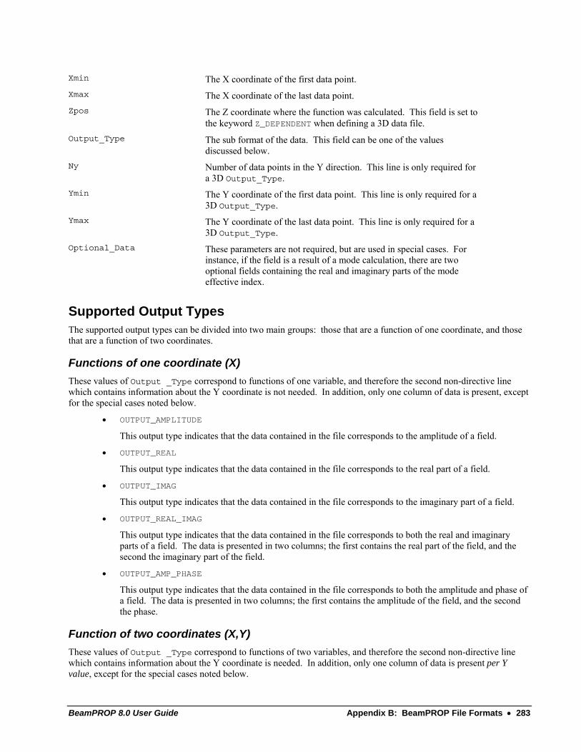
BeamPROP 8.0 User Guide Appendix B: BeamPROP File Formats • 283
Xmin The X coordinate of the first data point. Xmax The X coordinate of the last data point. Zpos The Z coordinate where the function was calculated. This field is set to
the keyword Z_DEPENDENT when defining a 3D data file. Output_Type The sub format of the data. This field can be one of the values
discussed below. Ny Number of data points in the Y direction. This line is only required for
a 3D Output_Type. Ymin The Y coordinate of the first data point. This line is only required for a
3D Output_Type. Ymax The Y coordinate of the last data point. This line is only required for a
3D Output_Type. Optional_Data These parameters are not required, but are used in special cases. For
instance, if the field is a result of a mode calculation, there are two optional fields containing the real and imaginary parts of the mode effective index.
Supported Output Types The supported output types can be divided into two main groups: those that are a function of one coordinate, and those that are a function of two coordinates.
Functions of one coordinate (X) These values of Output _Type correspond to functions of one variable, and therefore the second non-directive line which contains information about the Y coordinate is not needed. In addition, only one column of data is present, except for the special cases noted below.
• OUTPUT_AMPLITUDE
This output type indicates that the data contained in the file corresponds to the amplitude of a field.
• OUTPUT_REAL
This output type indicates that the data contained in the file corresponds to the real part of a field.
• OUTPUT_IMAG
This output type indicates that the data contained in the file corresponds to the imaginary part of a field.
• OUTPUT_REAL_IMAG
This output type indicates that the data contained in the file corresponds to both the real and imaginary parts of a field. The data is presented in two columns; the first contains the real part of the field, and the second the imaginary part of the field.
• OUTPUT_AMP_PHASE
This output type indicates that the data contained in the file corresponds to both the amplitude and phase of a field. The data is presented in two columns; the first contains the amplitude of the field, and the second the phase.
Function of two coordinates (X,Y) These values of Output _Type correspond to functions of two variables, and therefore the second non-directive line which contains information about the Y coordinate is needed. In addition, only one column of data is present per Y value, except for the special cases noted below.

284 • Appendix B: BeamPROP File Formats BeamPROP 8.0 User Guide
• OUTPUT_AMPLITUDE_3D
This output type indicates that the data contained in the file corresponds to the amplitude of a field.
• OUTPUT_REAL_3D
This output type indicates that the data contained in the file corresponds to the real part of a field.
• OUTPUT_IMAG_3D
This output type indicates that the data contained in the file corresponds to the imaginary part of a field.
• OUTPUT_REAL_IMAG_3D
This output type indicates that the data contained in the file corresponds to both the real and imaginary parts of a field. The data is presented in two columns per Y value; the first contains the real part of the field, and the second the imaginary part of the field.
• OUTPUT_AMP_PHASE_3D
This output type indicates that the data contained in the file corresponds to both the amplitude and phase of a field. The data is presented in two columns per Y value; the first contains the amplitude of the field, and the second the phase.
Functions of three coordinates (X,Y,Z) Functions of three coordinates are similar to the functions of two coordinates. The differences are:
• The keyword Z_DEPENDENT in the typical Z position field.
• An additional header line that defines the range of z data and the number of z slices is required (Nz Zmin Zmax)
• The data is given in matrices one after another corresponding to the multiple Z cross-sections. The actual user profile will interpolate between cross-sections in Z as it does between data points in X or XY.
See the example field below for the header/data structure.
Data Files with a Non-Uniform Grid The format described above describes a data file with a uniform grid. Data files with a non-uniform grid, such as index profiles produced using the CAD’s non-uniform grid options, have the same header lines described above, but the data has the following format:
0 Ymin … Ymax
Xmin Data1(Xmin, Ymin)
… Data(Xmin, Ymax)
… … …
Xmax Data(Xmax, Ymin)
… Data(Xmax, Ymax)
where the first column contains the X coordinates of each row of data, and the first line has the Y cooridnates of each column of data. The value 0 in the upper right corner is necessary as a spacer, though the value doesn’t necessarily have to be 0.
Example Files In order to better illustrate the field file format, several examples are given. In each case, a function will be given, and then a corresponding data file.
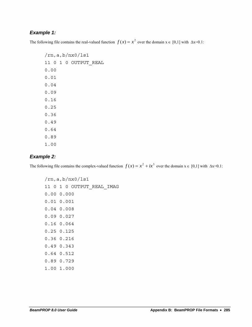
BeamPROP 8.0 User Guide Appendix B: BeamPROP File Formats • 285
Example 1:
The following file contains the real-valued function 2)( xxf = over the domain x ∈ [0,1] with Δx=0.1:
/rn,a,b/nx0/ls1
11 0 1 0 OUTPUT_REAL
0.00
0.01
0.04
0.09
0.16
0.25
0.36
0.49
0.64
0.89
1.00
Example 2:
The following file contains the complex-valued function 32)( ixxxf += over the domain x ∈ [0,1] with Δx=0.1:
/rn,a,b/nx0/ls1
11 0 1 0 OUTPUT_REAL_IMAG
0.00 0.000
0.01 0.001
0.04 0.008
0.09 0.027
0.16 0.064
0.25 0.125
0.36 0.216
0.49 0.343
0.64 0.512
0.89 0.729
1.00 1.000
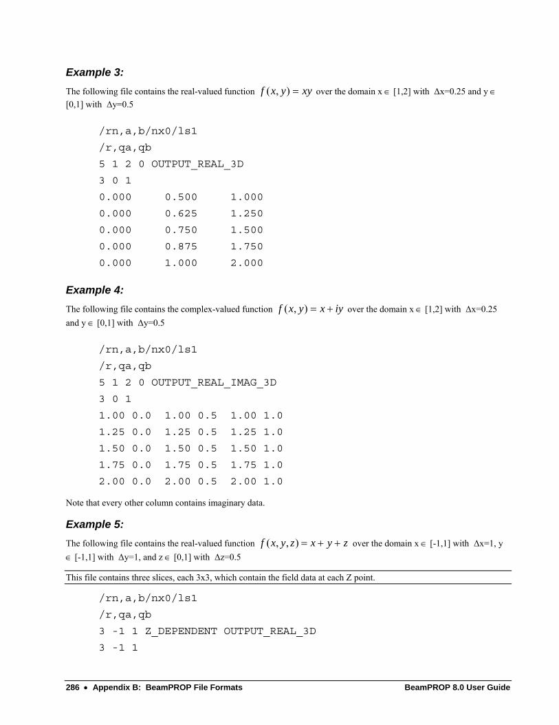
286 • Appendix B: BeamPROP File Formats BeamPROP 8.0 User Guide
Example 3: The following file contains the real-valued function xyyxf =),( over the domain x ∈ [1,2] with Δx=0.25 and y ∈ [0,1] with Δy=0.5
/rn,a,b/nx0/ls1
/r,qa,qb
5 1 2 0 OUTPUT_REAL_3D
3 0 1
0.000 0.500 1.000
0.000 0.625 1.250
0.000 0.750 1.500
0.000 0.875 1.750
0.000 1.000 2.000
Example 4: The following file contains the complex-valued function iyxyxf +=),( over the domain x ∈ [1,2] with Δx=0.25 and y ∈ [0,1] with Δy=0.5
/rn,a,b/nx0/ls1
/r,qa,qb
5 1 2 0 OUTPUT_REAL_IMAG_3D
3 0 1
1.00 0.0 1.00 0.5 1.00 1.0
1.25 0.0 1.25 0.5 1.25 1.0
1.50 0.0 1.50 0.5 1.50 1.0
1.75 0.0 1.75 0.5 1.75 1.0
2.00 0.0 2.00 0.5 2.00 1.0
Note that every other column contains imaginary data.
Example 5: The following file contains the real-valued function ( , , )f x y z x y z= + + over the domain x ∈ [-1,1] with Δx=1, y ∈ [-1,1] with Δy=1, and z ∈ [0,1] with Δz=0.5
This file contains three slices, each 3x3, which contain the field data at each Z point.
/rn,a,b/nx0/ls1
/r,qa,qb
3 -1 1 Z_DEPENDENT OUTPUT_REAL_3D
3 -1 1
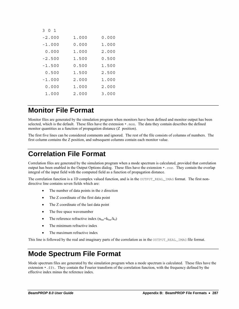
BeamPROP 8.0 User Guide Appendix B: BeamPROP File Formats • 287
3 0 1
-2.000 1.000 0.000
-1.000 0.000 1.000
0.000 1.000 2.000
-2.500 1.500 0.500
-1.500 0.500 1.500
0.500 1.500 2.500
-1.000 2.000 1.000
0.000 1.000 2.000
1.000 2.000 3.000
Monitor File Format Monitor files are generated by the simulation program when monitors have been defined and monitor output has been selected, which is the default. These files have the extension *.mon. The data they contain describes the defined monitor quantities as a function of propagation distance (Z position).
The first five lines can be considered comments and ignored. The rest of the file consists of columns of numbers. The first column contains the Z position, and subsequent columns contain each monitor value.
Correlation File Format Correlation files are generated by the simulation program when a mode spectrum is calculated, provided that correlation output has been enabled in the Output Options dialog. These files have the extension *.cor. They contain the overlap integral of the input field with the computed field as a function of propagation distance.
The correlation function is a 1D complex valued function, and is in the OUTPUT_REAL_IMAG format. The first non-directive line contains seven fields which are:
• The number of data points in the z direction
• The Z coordinate of the first data point
• The Z coordinate of the last data point
• The free space wavenumber
• The reference refractive index (nbar=kbar/k0)
• The minimum refractive index
• The maximum refractive index
This line is followed by the real and imaginary parts of the correlation as in the OUTPUT_REAL_IMAG file format.
Mode Spectrum File Format Mode spectrum files are generated by the simulation program when a mode spectrum is calculated. These files have the extension *.fft. They contain the Fourier transform of the correlation function, with the frequency defined by the effective index minus the reference index.
288 • Appendix B: BeamPROP File Formats BeamPROP 8.0 User Guide
Their format is similar to the field file format described above for the OUTPUT_AMPLITUDE case, except that the units are power not amplitude, and that the first non-directive line contains seven fields which are:
• The number of data points in the "frequency" (neff-nbar) direction
• The "frequency" coordinate of the first data point
• The "frequency" coordinate of the last data point
• The free space wavenumber
• The reference refractive index (nbar=kbar/k0)
• The minimum refractive index
• The maximum refractive index
This line is followed by the power spectrum as in the OUTPUT_AMPLITUDE file format.
Mode Results (Effective Index) File Format A mode result file (<prefix>.nef) is produced by BeamPROP whenever a mode compuation is performed. It contains a list of the modes found, and includes the mode number, the real part of the effective index, and the imaginary part of the effective index. Note that these values are the corrected values discussed in Section 6.D.2.
*.mds File Format A *.mds file contains raw data generated by the simulation program whenever any mode calculation is performed. The first non-directive line contains five fields which are:
• The number of modes found
• The free space wavenumber
• The reference refractive index (nbar=kbar/k0)
• The minimum characteristic refractive index.
• The maximum characteristic refractive index
This line is followed by a list of the mode information, each line corresponding to a mode. Each line has eight columns which represent the following data:
• The mode number, which simply enumerates the peaks from high to low frequency
• The mode effective index, given relative to the reference index (i.e. neff-nbar). This is the uncorrected value.
• The mode effective index, obtained by simply adding the reference index to the above. This again is an uncorrected value.
• The mode effective index, obtained more accurately through the ‘first correction’ discussed in Section 6.D.2. This field is the same as the above field for the iterative method.
• The normalized mode effective index (i.e. the so-called b parameter)
• The mode weight, given as a fraction of power in the input field (0 for iterative method)
• The imaginary part of the mode effective index. This is not valid in all cases and be set to 0. For example, the imaginary part is not calculated if only the mode spectrum is calculated as the method requires the mode profiles themselves be computed. Also, imaginary effective index output is disabled when the variable neff_method is set to 0.

BeamPROP 8.0 User Guide Appendix B: BeamPROP File Formats • 289
• The real part of the mode effective index as obtained via the ‘second correction’ described in Section 6.D.2. For the iterative method, this is just a duplicate of the 3rd and 4th columns. For the correlation method, this is the value found by substituting the mode profiles in the wave equation.
The values displayed in any output data or plot files will correspond to the values in the 7th and 8th columns.
Mode Field File Format Mode field files are generated by the simulation program when one or more modes are calculated. These files have the extension *.m##, where ## is the mode number. Their default format is identical to the field file format described above for the OUTPUT_REAL_IMAG or OUTPUT_REAL_IMAG_3D case.
This default can be changed via the output options dialog. Note that for mode field files, the optional fields in the field file format documented above are used, with the two optional fields containing the real and imaginary parts of the mode effective index. The effective index information is also stored and displayed in the corresponding *.p## graph file that is generated.
Refractive Index and Loss Profile File Formats Refractive index or loss profile files are generated by the simulation program when the index or loss profile is calculated. These files have the extensions *.ipf and *.lpf, respectively. They contain the real or imaginary part of the refractive index as a function of the transverse coordinates. Their format is similar to the field file format for the OUTPUT_REAL or OUTPUT_REAL_3D case.
Electrode/Heater Formats The Electrode/Heater utility in BeamPROP produces data files with extensions *.pv, *.pex, and *.pey and contain the transverse electric potential and electric fields due to the electrode/heaters in the design file. Their format is similar to the field file format for the OUTPUT_REAL_3D case.

BeamPROP 8.0 User Guide Appendix C: Symbol Table Variables • 291
Appendix C: Symbol Table Variables
In this appendix we document the symbol table variable names which control the internal operation of BeamPROP. Most of these variables correspond to dialog fields which have already been documented.
The following table lists the variable names corresponding to these dialog fields.
BPM Simulation Parameters The following variables correspond to the fields found in the BPM Simulation Parameters dialog box: Field Name Variable
X Domain Min boundary_min
X Domain Max boundary_max
X Grid Size grid_size
X Slice Grid slice_grid_size
Y Domain Min boundary_min_y
Y Domain Max boundary_max_y
Y Grid Size grid_size_y
Y Slice Grid slice_grid_size_y
Z Domain Min domain_min
Z Domain Max domain_max
Z Grid Size step_size
Z Slice Grid slice_step_size
Z Monitor Grid monitor_step_size
Display Mode slice_display_mode
Output File Prefix prefix
292 • Appendix C: Symbol Table Variables BeamPROP 8.0 User Guide
Advanced Grid Parameters The following variables correspond to the fields found in the Advanced Grid Parameters dialog box that have not documented in the last section:
Field Name Variable Name X Grid Size (Bulk) grid_size
X Grid Size (Edge) grid_edge_x
X Griding Ratio grid_ratio_x
X Minimum Divisions grid_mindiv_x
X Grid Grading grid_bulk_nonuniform_x
X Interface Alignment grid_align_x
Y Grid Size (Bulk) grid_size_y
Y Grid Size (Edge) grid_edge_y
Y Griding Ratio grid_ratio_y
Y Minimum Divisions grid_mindiv_y
Y Grid Grading grid_bulk_nonuniform_y
Y Interface Alignment grid_align_y
Z Grid Size (Bulk) step_size
Z Grid Size (Edge) grid_edge_z
Z Griding Ratio grid_ratio_z
Z Minimum Divisions grid_mindiv_z
Z Grid Grading grid_bulk_nonuniform_z
Z Interface Alignment grid_align_z
Advanced Numerical Parameters The following variables correspond to the fields found in the Advanced Parameters dialog box: Field Name Variable
Numerical Scheme scheme
Boundary Condition bc_type
Boundary Location boundary
Boundary Gap boundary_gap
Scheme Parameter scheme_parameter
Padé Order pade_order
Reference k kbar
Reference k Value kbar
Reference k Angle kbar_angle
BeamPROP 8.0 User Guide Appendix C: Symbol Table Variables • 293
Reference k Angle Value kbar_angle
Bi-Directional Parameters The following variables correspond to the fields found in the Bi-Directional Parameters dialog box: Fieldname Variable
Operator bd_operator
BD Pade Order bd_pade_order
Imag Parameter bd_imag_parameter
Iteration bd_iteration
Tolerance bd_tol
Max Iterations bd_max_iterations
Damping Factor bd_damp_factor
Display Options The following variables correspond to the fields found in the Display Options dialog box: Field Name Variable
Slice Colors color_slices
Circuit Color color_circuit
Slice Normalization slice_normalization
Slice Position X slice_position_x
Slice Position Y slice_position_y
Monitor Complement monitor_complement
Monitor Log Scale monitor_log_scale
Monitor Range Min monitor_min
Monitor Range Max monitor_max
Index Min index_min
Index Max index_max
Surface Color color_surface
Outline Color color_outline
View Phi view_phi
View Theta view_theta
Color Shades color_shades
Color Scale color_scale
Show Color Scale color_scale_display
Allow Redraw 2D allow_redraw_2d
Allow Redraw 3D allow_redraw_3d

294 • Appendix C: Symbol Table Variables BeamPROP 8.0 User Guide
Plot Aspect Ratio plot_aspectratio
Output Options The following variables correspond to the fields found in the Output Options dialog box: Field Name Variable
Slice Output Format slice_output_format
Field Output Format field_output_format
Mode Output Format mode_output_format
Far Field Output farfield_output
Monitor Output monitor_output
Correlation Output correlation_output
Run Log Output run_output
Launch Parameters The following variables correspond to the fields found in the Launch Parameters dialog. Note that this is only valid for the specification of one launch field. Multiple launch fields are specified directly in the *.ind file. Field Name Variable
Launch Pathway launch_pathway
Launch Type launch_type
Launch Tilt launch_tilt
Launch Polarization launch_polarization
Launch Mode launch_mode
Launch Mode Radial launch_mode_radial
Random Set random_set
Input File (E-Major) launch_file
Input File (E-Minor) launch_file_minor
Launch Normalization launch_normalization
Launch Background N launch_background_index
Launch Delta N launch_delta
Launch Angle launch_angle
Launch Width launch_width
Launch Height launch_height
Launch Position X launch_position
Launch Position Y launch_position_y
Launch Neff launch_neff
Launch Align File launch_align_file
BeamPROP 8.0 User Guide Appendix C: Symbol Table Variables • 295
Launch Power launch_power
Launch Phase launch_phase
Mode Solving The following variables correspond to the mode solving features discussed in Chapter 6.
Mode Calculation Options The following variables correspond to the fields in the Mode Calculation Options dialog: Field Variable
Method mode_method
Neff Log neff_log
Neff Tolerance neff_tol
Neff Min char_nmax
Neff Max char_nmin
Advanced Mode Solving Features The following variables correspond to advanced mode-solving features discussed in Chapter 6: Variable Description
mode_threshold The minimum threshold above which modes peaks are found from a mode spectrum.
idbpm_convergence_warning Toggles on/off the warning that an iterative mode calculation has not converged.
mode_spectrum Indicates that a mode spectrum should be computed. mode_set Indicates the modes to be solved for. idbpm Computes fundamental mode. step_size_idbpm Z Compute Step for mode calculations. step_size_idbpm_factor The safety factor used to determine the default step sized used for
iterative mode solving calculations. This factor should normally be less than one, and defaults to 0.5.
mode_length Sets the domain length for a mode calculation. neff_tol_cor Sets the desired tolerance for the effective indices for a correlation
mode solving calculation. neff_scan_output Sets the type of output for a mode scan. Setting this parameter to 0
disables output, 1 enables output of real indices, and 2 enables output of real and imaginary indices.
Boundary Conditions The following variables correspond to different boundary conditions:
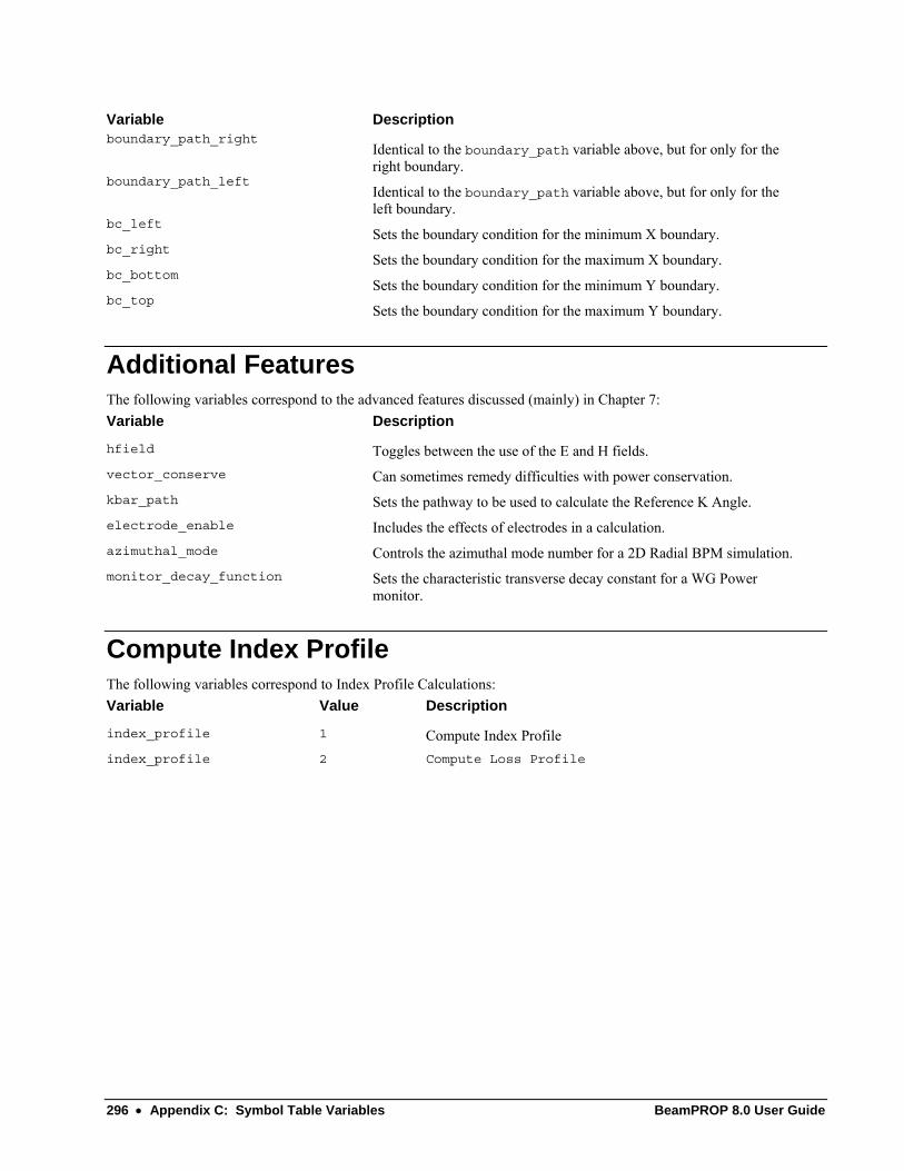
296 • Appendix C: Symbol Table Variables BeamPROP 8.0 User Guide
Variable Description boundary_path_right
Identical to the boundary_path variable above, but for only for the right boundary.
boundary_path_left Identical to the boundary_path variable above, but for only for the left boundary.
bc_left Sets the boundary condition for the minimum X boundary.
bc_right Sets the boundary condition for the maximum X boundary.
bc_bottom Sets the boundary condition for the minimum Y boundary.
bc_top Sets the boundary condition for the maximum Y boundary.
Additional Features The following variables correspond to the advanced features discussed (mainly) in Chapter 7: Variable Description
hfield Toggles between the use of the E and H fields. vector_conserve Can sometimes remedy difficulties with power conservation. kbar_path Sets the pathway to be used to calculate the Reference K Angle. electrode_enable Includes the effects of electrodes in a calculation. azimuthal_mode Controls the azimuthal mode number for a 2D Radial BPM simulation.monitor_decay_function Sets the characteristic transverse decay constant for a WG Power
monitor.
Compute Index Profile The following variables correspond to Index Profile Calculations: Variable Value Description
index_profile 1 Compute Index Profile index_profile 2 Compute Loss Profile
BeamPROP 8.0 User Guide Appendix D: BeamPROP Release Notes • 297
Appendix D: BeamPROP Release Notes
This appendix summarizes the changes from previous versions of BeamPROP. Additionally, since the documentation for the RSoft CAD Layout tool was found in the BeamPROP manual prior to version 5.1, changes in the CAD are also found in this section.
Within each section, the first subsection discusses new or improved features, and the second subsection covers compatibility issues.
Changes from Version 7.0 to Version 7.1 Note that the change log which details the history of changes from Version 7.0 to Version 7.1 is available in the file README71.TXT.
New Capabilities and Improvements to the Program
CAD: • Improved CAD interface. See CAD manual for more details.
Significant Changes in Program Behavior • Added a control for the H-field formulation in the Advanced Parameters dialog.
• Moved polarization and vector mode options to the Simulation Parameters dialog.
• The bidirectional options are now accesible from the Advanced Options dialog.
Changes from Version 6.0 to Version 7.0 Note that the change log which details the history of changes from Version 6.0 to Version 7.0 is available in the file README70.TXT.
298 • Appendix D: BeamPROP Release Notes BeamPROP 8.0 User Guide
New Capabilities and Improvements to the Program
CAD: • Introduction of an entirely new index/grid/mesh generation algorithm which improves accuracy and allows
more flexible layout.
• Added support for non-uniform grids. This can significantly improve accuracy while improving simulation speed.
• Integrated BeamPROP with the Material Editor.
Simulation: • Improved the convergence of the iterative mode solver in some cases.
Other: • Improved dialog for mode computation.
Significant Changes in Program Behavior • Addition of new output file for mode calculations which simplifies the output of mode effective indices.
The new file is named <prefix>.nef.
• Changed the default number of grid points used for the slice grid.
Changes from Version 5.1 to Version 6.0 Note that the change log which details the history of changes from Version 5.1 to Version 6.0 is available in the file README60.TXT.
New Capabilities and Improvements to the Program
CAD: • Correction to index profile for overlapped channel waveguides with negative side slope. Previously, in
some cases, this combination could yield cutoff portions of the channel. The problem has been corrected.
Simulation: • A new simulation variable, step_size_idbpm_factor, has been added. For the iterative mode
calculation method, the default step size is determined from a theoretical ideal, and multiplied by a safety factor (which should normally be less than one). The safety factor was fixed at 0.5, but can now be changed.
• A new simulation variable, mode_length, has been added. This variable sets the length for mode calculations independently of Z Domain Max.
• A new feature to output the imaginary part of the effective index calculated during a mode scan. Normally, only the real part of neff is output. By setting the variable neff_scan_output to the value 2 in the symbol outputs, the imaginary part will be output as well.
BeamPROP 8.0 User Guide Appendix D: BeamPROP Release Notes • 299
Analysis/Results: • Extension of far field output option to include phase.
• New option to output the H field when doing mode calculations via the variable hfield_output.
• A change to the output of the .mds file which accomplishes several things. First, the precision of some columns is improved. Second, the file now regularly includes the 7th column for the imaginary part. Note, however, that this will not be valid in some cases and will just contain 0. Third, the file now includes an 8th column which is the real part of neff.
• Enabled output of imaginary part of index profile for Anisotropic case. Note that to enable output of all tensor components, index_profile_all=1 must be set.
Other: • A small correction to the stargen utility for AWG layout.
• Corrected an error in the disperse utility which produced incorrect results for some combinations of options.
Significant Changes in Program Behavior • The vector_conserve option, introduced in Version 5.0, has been enabled by default and added to the
Advanced Parameters dialog. The default for this option may be changed by the user by setting VectorConserve=1 in the [BSIM] section of the BCADW32.INI file.
• A new method for overlap power calculations in 3D vector BPM has been introduced. This method applies a more rigorous vector formulation to determine overlap integrals, and is enabled by default. If necessary, this method may be disabled by setting overlap_eh=0 in the symbol table for an individual .ind file, or setting OverlapEH=0 in the [BSIM] section of the BCADW32.INI file to disable it by default.
• A change in power calculations for full vector BPM. The new method calculates power more accurately for large minor component, and separates major and minor components of the power in a more useful way.
• Added an option to exclude the boundary points in power or overlap calculations. Rigorously, the theorems for power conservation in BPM exclude the boundary points, however in practice the normally do not contribute significantly. However, in some rare cases, these points can diverge briefly, and the power reported by BeamPROP demonstrates a spike. The new option avoids this problem by excluding these points, and is enabled by default. To disable it, you can set overlap_exclude_boundary=0 in the symbol table of an individual .ind file, or OverlapExcludeBoundary=0 in the [BSIM] section of the BCADW32.INI file to turn it off by default.
• Added an option to improve mode convergence in some cases. Previously, in rare cases, the iterative method would prematurely converge and yield an unphysical value for the effective index. The new option neff_clip=1can be used to avoid this problem. Note that it should only be used if there appears to be a problem, since it can exclude valid modes in some cases.
Changes from Version 5.0 to Version 5.1 Note that the change log which details the history of changes from Version 5.0 to Version 5.1 is available in the file README51.TXT.

300 • Appendix D: BeamPROP Release Notes BeamPROP 8.0 User Guide
New Capabilities and Improvements to the Program
CAD: • Improved export of components employing the new Segment Orientation feature. Previously, these were
only exported correctly if the Export Polygon Mode was Raw; otherwise they were exported more or less as if the Segment Orientation had been ignored. Now they are exported correctly in all cases, however Raw export is always a truer representation but may exceed the 200 point GDS-II polygon limit.
• A new GDS-II import option. Note that the importer does not currently support PATH and NODE elements.
• Support for LWPOLYLINE in DXF import and an improvement allowing import of closed polylines which are missing the final point.
• Improved clipping of objects in the CAD an simulation windows.
• A feature for easier editing of 3D structures involving overlapping components in different y planes using the variable cad_yselect_size.
• Export of concave lens objects has been corrected.
• Updated the Symbol Table Editor dialog to have a wider window for displaying the current value. This avoids cutting off the display of very small or large numbers that need to be shown in scientific form.
• New functions that can be used in expressions for generating random sequences and lines.
Simulation: • Performing a Mode Spectrum scan has been altered to allow the range of modes (i.e. Mode Set) to be
selected. When this is done, only these modes will be output to the .nes/.pne file for the effective index data.
Analysis/Results: • A new option in the scan variable dialog called "Plot Dynamically". This option causes the results of a
single variable scan to be displayed and updated dynamically as each run is completed. Depending on user feedback, this option may become the default.
• The WDM Router Simulation dialog now generates additional scripts.
• Added rotation option to BDUTIL.EXE.
Other: • Updated the XZ and XYZ array generators to enable producing layouts centered at z=0 rather than starting
at z=0.
• Increased the maximum allowed characters per line in WinPLOT to 80,000 from 16,000. This will allow larger data files to be opened in WinPLOT.
• The EXAMPLES directory has been restructured so that it no longer contains any files directly.
• RSoft has developed data file converters between BeamPROP and Zemax, similar to the existing converters between BeamPROP and CODEV. While these will be officially released in an upcoming version, any user requiring these converters may contact RSoft to obtain them by email.
Significant Changes in Program Behavior • Faster calculation for 3D simulations with large numbers of fiber or channel structures (e.g. PBG fibers).

BeamPROP 8.0 User Guide Appendix D: BeamPROP Release Notes • 301
• A new option which allows mode calculations via the correlation method to calculate the imaginary part of the effective index if the mode is leaky. Even for normal guided modes, the new option generally results in slightly more accurate values for the effective index. The new option is enabled by default, but can be controlled by the variable neff_method.
• For radial simulations, updated the 1/e monitor to calculate the width of the field in full Cartesian coordinates, and not in radial coordinates. The monitor will now give values which are double the values obtained with the previous versions. If you experience any difficulty with this new method, please contact RSoft.
• Improvements to the licensing mechanism, especially in the case of Network licenses which now allow multiple copies of the CAD program to be opened on the same machine, even when only one license is available.
• Changed the behavior of the SaveAs dialog to change the working directory to the specified directory.
• The electronic licensing mechanism has been updated. Now all licensing is done through license files which must be obtained by email from RSoft ([email protected]).
• Distribution of new code based on DLL's. This is being done to enable more dynamic updates of dialogs for addons such as BandSOLVE and GratingMOD.
• A major update to the launch capabilities has been made.
• An error which would cause the program to crash if the number of modes found in the iterative method exceeded the maximum mode limit has been corrected. The program will now simply terminates gracefully after finding the largest mode allowed, and prints a warning message to the log file. If more modes are desired, you can change the limit as noted above.
• A change in the behavior of the scan dialog to warn if the scan variable does not exist (or is not an internal variable). This warning can be disabled by setting scan_variable_warning=0.
Changes from Version 4.0 to Version 5.0 Note that the change log which details the history of changes from Version 4.0 to Version 5.0 is available in the file README40.TXT.
New Capabilities and Improvements to the Program
CAD: • Added a major new feature to allow BeamPROP's generalized segment (including most tapers and arcs) to
have a reference orientation along the axis of the segment. Use of this feature provides a means of achieving geometries or effects which were previously awkward or impossible to obtain, including arbitrary segment rotation, endfaces perpendicular to the segment, width tapers referenced to the segment axis, and arcs up to 90 degrees which maintain shape and endface orientation.
• Implemented use of the above in the layouts generated by the WDM Router (AWG) module.
• Eliminated arbitrary limitations on the number of components (previously limited to 20,000).
• Added improvements to the XZ array layout utility, particularly useful for PBG applications in FullWAVE
• Introduced a new XYZ array layout utility, particularly useful for PBG applications in FullWAVE
• The number of user tapers/profiles has been increase to 16 each, and the CAD interface for accessing them has been improved.
• The number of symbols has been increased from 2048 to 3000, and it use configurable if necessary.

302 • Appendix D: BeamPROP Release Notes BeamPROP 8.0 User Guide
• The Polygon and Lens dialogs have been expanded to allow additional control over these objects.
• Added CAD import options for DXF and CIF files.
Simulation: • Implemented a major new feature for "Simulation Regions", which allows, among other things, local
control of many simulation options along z. These include step size, reference k value and angle, Pade order, simulated bend options, and propagation scheme. This feature is discussed in the BeamPROP manual.
• Added an FFT-based BPM which can be used in conjunction with the above for certain special circumstances.
• Added nonlinear capability to 3d for Fiber/Channel structures.
• Added a new option which enables an improved vector BPM that handles a wider range of problems.
• Improved and extended the WGMODE command line program for analyzing simple waveguide structures.
• Improved robustness of the programs parameter estimation.
• Improved logic of the program if the user specifies a domain and grid which are not evenly divisible.
• Several limitations of the PHASECOR component of the AWG design module were removed.
• Corrected a problem in the AWG design capability which occurred when the user incorrectly selected TM in the global settings to attempt to account for polarization. As noted in the AWG documentation, the correct approach is to use the “design” variables described there.
• The command line length allowed in script processing has been increased from 256 to 1024.
• The "radial" variable has been added as an alternate way of specifying Radial BPM (for consistency with FullWAVE).
• Added a new option to disable convergence warnings during iterative mode calculation.
• Extended the Combine Mode Add option to allow the addition of standard index profiles for Fiber, Channel, and Diffused structures to any other structure (previously only user profiles could be added). This allows, for example, more convenient mixing of diffused and multilayer structures.
• Added a new capability to allow fiber and channel components to have their own “delta tensor”. This feature is accessed via the More… dialog of the component properties dialog. Coupled with Combine Mode Add and user profiles, by overlapping multiple waveguides this feature allows different index profiles for different components of the index tensor.
• Improved the calculation of diffused index profiles at substrate/cover interfaces.
• The bdutil BeamPROP data file manipulation utility has been updated to include a new option (-k) for calculating coupling coefficients. Type "bdutil" at the command line to see the new command line options. This feature is also accessed via the new grating analysis feature that is accessed via the Utility/Grating… menu item.
• Added a new utility, grutil, for performing simple grating analysis. Type "grutil" at the command line to see the usage for this utility. This feature is also accessed via the Utility/Grating… menu item.
• General speed improvements.
Analysis/Results: • Added a capability to the WG Power monitor option in 3D to allow the user to choose whether the power
should be integrated over a rectangular or elliptical cross-section.
• Improved power and overlap calculation for 3D vector field calculations.
BeamPROP 8.0 User Guide Appendix D: BeamPROP Release Notes • 303
• Added an option to output Radial BPM results as 3D data files and graphs.
• Added a new option to enable storing of both XZ and YZ data simultaneously when doing a 3D simulation and saving results.
• Added a fixed aspect ratio option to various plots. The option is available under the Display... button. For stored plots generated with previous versions, or generated without having set this option, the aspect ratio can be changed in WinPLOT under Options/Axes/Aspect-Ratio… or via the /aspect option.
• The dispersion utility has been updated with new options to compute derivatives of Beta instead of Neff and with respect to wavenumber instead of wavelength, as will as an option to compute group velocity and dispersion as a function of wavelength. Type "disperse" at the command line to see the new command line options.
Other: • Updated the main documentation and included a new consolidated and improved version of the AWG
Utility documentation.
• Included a new version of WinPLOT (2.5) which, among other things, has a toolbar which allows convenient switching between the edit and plot windows.
Significant Changes in Program Behavior • The method for calculating powers and overlap integrals for 3D vector field calculations has been
improved. This may cause some change in results depending on the problem. Contact RSoft with any questionable change in behavior.
• The default behavior of the WG Power monitor option has been changed in the case of Fiber structures. Previously, the WG Power monitor would integrate the power over a rectangular cross section, independent of the waveguide geometry. Now, if the geometry of the waveguide in the pathway being monitored is a Fiber, the program will integrate over an ellipse (or circle if the width and height are equal). This change in behavior will cause different results, so if you have files which use Fibers and WG Power, they may need to be changed if you prefer the old definition. The monitor dialog now has an option called Monitor Shape to control this.
• The method for calculating diffused index profiles at substrate/cover interfaces has been improved, however it should be noted that this may cause previous results to change if the grid size used was coarse (if the grid size used was sufficiently fine, the results should be essentially the same). While the new behavior should be more accurate, the old behavior can be recovered by setting diffusion_intavg to 0 in the symbol table.
• The old method for selecting Radial BPM, namely through the Numerical Scheme in the Advanced Parameters dialog, has been removed. Files which use this option will automatically be converted where appropriate to use the new "radial" variable introduced in 4.0f, which is also selected in the Global Settings.
• The log file has been renamed to log.txt for compatibility with other RSoft programs.
• The location of the INI file holding the window size and other settings has been changed to the users home directory under Windows NT/2000/XP. This avoids permission problems that sometimes occurred with this file and also allows different users to have different preferences.
• The default color map for WinPLOT line drawings has been changed. The new map avoids the use of harder to see colors and addresses other issues. The old map can be recovered via the /lcm option in the plot.cfg file.
• Internal changes to script processing were made for general improvement. This may cause problems if DOS batch files or rarely used commands were called from BeamPROP scripts. If this is the case, contact RSoft to see if there is a workaround.

304 • Appendix D: BeamPROP Release Notes BeamPROP 8.0 User Guide
Changes from Version 3.0 to Version 4.0 Note that the change log which details the history of changes from Version 3.0 to Version 4.0 is available in the file README30.TXT.
New Capabilities and Improvements to the Program • The electrode/heater feature has been extended to recognize anisotropic dielectric constants or thermal
conductivities.
• An option (electrode_enable) has been added to allow control the automatic electrode calculation feature.
• The electrode/heater feature has been extended to partially allow for tilted/curved structures.
• The wide-angle feature has been partially enabled for 3D.
• New iteration schemes have been added to the bidirectional calculation feature.
• The ContourMap(XZ) display option has been enabled for the bidirectional calculation feature, and displays the sum of the forward and backward fields.
• The precision of the scan output files has been increased.
• A new utility, DISPERSE.EXE, has been added to calculate dispersion from the results of an effective index versus wavelength scan.
• The behavior of the Run menu items and green light icon have been improved to retain default behavior that has been explicitly selected by internal options such as idbpm=1.
• The storage of data for 3D graphics has been turned on by default.
• A new diffused waveguide option has been added, diffusion_gamma, which provides additional control over the diffusion profile shape.
• A new option, Options/Import-Symbols, has been added to allow symbol table information from another file to be imported into the current circuit. One use of this feature is to allow construction of material databases that can be imported into a circuit. An example has been created for TiLiNbO3 in TiLiNbO3.ind, which is documented in TiLiNbO3.doc in the examples directory.
• The Launch Computed Mode option has been corrected to function with the scan feature.
• The scan feature has been extended to automatically produce neff versus the scan parameter when a mode calculation option is selected. The results are stored in prefix.nes (data) and prefix.pne (plot).
• The scan dialog now has an option to select the run type (e.g. propagation or mode calculation).
• An option, electrode_a, has been added to control the acceleration parameter in the electrode/heater feature calculation.
• The router design feature has been updated with a new interface. See Router.doc in the router directory for a description of the new procedure.
• The Run/Run-Script option has been added to allow running BeamPROP script files from inside the CAD program in addition to from the command line.
• Improvements to the nonlinear calculation option at high intensities, including a new nl_iterations option to control the iteration procedure in nonlinear calculations.
• An option for saturable nonlinearities has been added under the More… dialog of the component properties dialogs.
• An option for locking the aspect ratio has been added under View/Set-View-Parameters.

BeamPROP 8.0 User Guide Appendix D: BeamPROP Release Notes • 305
• A field in the symbol table editor has been added which shows the current value of an expression.
• The labels for the imaginary part of the index of refraction have been changed from "Loss Coefficient" to "Index (imag)" to clarify their meaning.
• Access to the More… dialog has been added to the Polygon and Lens elements.
• The maximum number of pathways and monitors has been increased from 32 to 200. The maximum number of components in a pathway has been reduced from 1000 to 200.
• The maximum number of characters in an expression has been increased from 64 to 80.
• Several new function calls have been added. See Appendix for more details.
• The constants "pi" and "e" have been added for use in expressions.
• A radial BPM option has been implemented, which is selected under the Numerical Scheme in the Advanced… section of the simulation dialog. This option can be used to simulate circularly symmetric structures, such as fibers, in 2D rather than 3D. In conjunction with the bidirectional option it can be used to simulate properties of some fiber bragg gratings.
• The Generalized Douglas (CN) scheme, which can sometimes lead to higher accuracy than the Crank-Nicholson (CN) scheme, has been implemented in the 2D, TE case.
• All of the LP fiber modes have been implemented in the launch and monitor dialogs.
• The multimode launch option now functions in 3D, and launches a random combination of LP fiber modes.
• The automatic far field option now applies to the field output in propagation mode as well as in mode calculations.
• The accuracy of far field calculations has been improved, and a new option, farfield_da, has been added to control the accuracy.
• Redraw of circuits with complicated formulas, such as router layouts, has been improved.
• Calculation speed has been improved for various specific structure types.
• The program now stores different step sizes for propagation (step_size) and iterative mode calculation (step_size_idbpm).
• A warning has been added when the iterative mode calculation does not converge.
• New icons have been added in the simulation part of the toolbar.
• Tooltips have been added to the icons in the toolbars.
• In Run Logs, the Ref k Value is now stored as kbar_value, while kbar is retained as originally set.
• A warning has been added to remind users to edit tapers and profiles via the Edit/Tables/… menu.
• For convenience the variable "k0" is now predefined in new circuits to be "(2*pi)/free_space_wavelength". This is mostly of use when defining a Ref k Value to correspond to an effective index as in "k0*Neff".
• A new option has been added under the Edit menu to allow selection/editing of a component by its number, which is useful for components that are "buried" under other overlapping components.
• An option has been added to allow 2D mode fields (coming from radial BPM for example) to be used as launch fields for 3D calculations.
• When an iterative mode calculation is performed, the imaginary part of the index is reported if present.
• The mode effective index is now stored in mode field files, and is used, for example, when a mode field is launched from a file at a tilted angle.
• The length of script files is now unlimited.

306 • Appendix D: BeamPROP Release Notes BeamPROP 8.0 User Guide
• The maximum number of symbols has been increased to 2048.
• The maximum number of electrode groups has been increased to 32.
• Deletion of components now maintains component ordering (component references were always maintained, but so-called depth-ordering would be modified).
• Options have been added under Edit/Change-Order to change the so-called depth-ordering of components.
• Several options have been added to provide an interface to FullWAVE, most notably the FDTD calculation in the startup dialog, and the corresponding simulation dialog that is invoked by the green light when in FDTD calculation mode. In addition, the Options/Insert/Time-Monitor menu item has been added.
• An option to produce registration marks for CAD export has been added under Options/Insert/Mark.
• The Channel structure now has an option (under the More… dialog) for obtaining sloped sidewalls.
• Various improvements and new features to the router design have been made. Refer to Router.doc in the router directory for more details.
• Several new utilities have been added under the Utility menu for creating arrays of waveguides in (XZ) or (XY) for use with photonic bandgap crystals and photonic bandgap fibers.
• A new ContourMap(YZ) display option has been added.
• The display of index profiles has been modified so that if an option other than Fixed at Z-Min is selected, the index instead of the height is plotted. A new option SurfaceRelief recovers the previous behavior.
• Several new color scales have been added.
• Several new options to WinPLOT have been added. These are documented in the README.RPL file.
• The default output option for storing slices has been changed to reflect more common usage. Now, storing of slices is disabled by default in the case of either mode calculations or when using the ContourMap(XY) display mode. Storing slices can be re-enabled via the output options dialog.
• The launch capabilities have been extended to allow multiple launch fields.
• The default vertical positioning of the monitor field has been changed in the case of a monitor type of File so as to attempt to automatically align with the pathway being monitored. Previously, only the horizontal position was automatically aligned.
• An option has been added (launch_align_file=1) to force alignment of the launch field with the pathway being launched into in the case of a launch type of File or (Computed Mode since it is based on File). Other launch types have always been and continue to be automatically aligned, independent of the setting of this new option.
• The launch and monitor polarization options (which only affect 2D slab modes) have been extended to include a Default option, which automatically adapts to the polarization setting in the global settings dialog. This changes the default behavior and may effect some existing .ind files if they were improperly set to begin with.
• The default options for bidirectional simulation in the TM case have been changed to use the undocumented hfield option, as is required for proper simulation in the bidirectional TM case.
• A new arc type has been added. The new Final Angle option complements the operation of the previously existing Initial Angle option.
• A new option controlling whether the lens object represents a cylindrical lens (the default) or a spherical lens, has been added to the lens properties dialog.

BeamPROP 8.0 User Guide Appendix D: BeamPROP Release Notes • 307
Significant Changes in Program Behavior • The default mode calculation option has been changed from the correlation method to the iterative method.
The correlation method can be selected explicitly via Run/Compute-Mode/Options and will be retained when the .ind file is saved.
• The Windows version of RPlot, WINPLOT.EXE, has been changed so that viewer mode is now the default and the /v option is unnecessary. To run the program in edit mode use the new /e option as in "winplot /e".
• The initialization file has been renamed from BCADWIN.INI to BCADW32.INI
• In the startup dialog the Save Settings box is now off by default.
• The option to show color scales has been turned on by default.
• The default coarse color scale has been changed to have 10 levels instead of 11, and more accurately correspond to the default continuous scale.
• The default waveguide display has been changed to Both from Center/Outer (see Options/Preferences dialog).
• The Run Log Output has been turned on by default.
• The default output option for storing slices has been changed to reflect more common usage. Now, storing of slices is disabled by default in the case of either mode calculations or when using the ContourMap(XY) display mode. Storing slices can be re-enabled via the output options dialog.
• The default vertical positioning of the monitor field has been changed in the case of a monitor type of File so as to attempt to automatically align with the pathway being monitored. Previously, only the horizontal position was automatically aligned.
• The launch and monitor polarization options (which only affect 2D slab modes) have been extended to include a Default option, which automatically adapts to the polarization setting in the global settings dialog. This changes the default behavior and may effect some existing .ind files if they were improperly set to begin with.
• The default options for bidirectional simulation in the TM case have been changed to use the undocumented hfield option, as is required for proper simulation in the bidirectional TM case.
• The behavior of user profiles has been changed. Previously, when a user profile was used which had higher priority than other waveguides, it would dominate the index profile, causing other waveguides to disappear. Now, only if the value of the user function is nonzero will it dominate. This new behavior matches what is most likely intended, however it may cause some existing .ind files to function differently. If this is the case, contact RSoft for a workaround.
• The interpretation of data files in the simulation program and various utilities has been modified so that outside the domain of definition, the function is defined to be zero, rather than an extension of the boundary data. In most cases, the data in a file would be near zero anyway and this will not matter, however we find this new behavior to be beneficial in many instances (for example if a mode is calculated on a domain which is not quite large enough, stored to a file, and then launched into the program). Contact RSoft if you notice any difficulties which appear to be related to this new behavior.
• The step size used for propagation and the step size used for iterative mode calculation have been fully separated. Previously, if the step size for iterative mode calculation had not been changed from the default, but the step size for propagation had, the propagation step size would be used for the iterative mode calculation. Now, if the step size for iterative mode calculation has not been changed from the default it will use the proper default, independent of the setting for the propagation step size.

308 • Appendix D: BeamPROP Release Notes BeamPROP 8.0 User Guide
Changes from Version 2.1 to Version 3.0
New Capabilities and Improvements to the Program • A major new feature for bidirectional BPM, which accounts for reflections, has been added. A new
example file, GRATING.IND, is included.
• A major new feature for nonlinear BPM has been added.
• A major new feature for calculating the effects of electrodes/heaters on the index profile has been added. A new example file, ELECTROD.IND, is included.
• A new launch option for automatically computing a mode and launching it into a circuit (Launch Computed Mode).
• A new launch option for controlling the normalization of the input field.
• A new monitor type for calculating the overlap with the input field.
• A new monitor type for calculating the mode effective index when doing an iterative mode calculation. This is useful when doing a parameter scan to get a plot of the effective index versus some parameter.
• Two new monitor types for calculating the 1/e width and height of the field.
• A new monitor option for controlling monitor normalization.
• A new monitor option for monitoring the power in a selected range of layers in a Multilayer structure.
• Improved expression handling with regard to operator precedence.
• Two new functions, step(x) and step2(x,a), which are useful for defining grating structures or segmented waveguides.
• A new option for controlling the vertical profile for Diffused structures (diffusion_shape).
• When selecting the RPlot graph icon in BeamPROP, the Files of type field lists the available graph types.
• The simulation program now indicates the coordinates of the cursor in its titlebar, which is useful for determining monitor values or other coordinates.
• The Outline Color option in the display options dialog has been expanded to show the circuit outline in the ContourMap(XZ) display mode, as well as the cross-section outline in the ContourMap(XY) display mode.
• A new feature for displaying an “isometric” plot of the index profile.
• A new display mode, 3D Slices, has been added.
• An option for viewing horizontal and vertical cuts of contour plots.
• An option for enabling/disabling the saving of settings in the startup dialog.
• The scan variable feature has been extended to allow negative going scans.
• The scanning of two variables has been improved so that separate .scn files are generated for each value of the outer iteration variable.
• A new conversion utility, mat2bp, has been added, and the previous conversion utility, bdconv, has been expanded.
• A new utility, bdutil, is included which can perform power calculations, overlap integrals, field size measurements, and far field calculations.
• The iterative mode solver has been extended for higher order modes.
• A new mode options dialog has been added to allow control over several mode calculation options.
BeamPROP 8.0 User Guide Appendix D: BeamPROP Release Notes • 309
• An output option for automatically computing the far field after a mode calculation has been added.
• The Multilayer option has been enhanced to allow arbitrary tapering of individual layers.
• A new option for duplicating Multilayer layer tables and layer taper tables has been added.
• The priority level option has been extended to different structure types.
• The waveguide display color option has been extended to use the display color in the CAD program as well as the simulation program.
• A new option to allow different waveguide components to be assigned different mask layers when exporting to a standard CAD file.
• The maximum number of components allowed in the CAD tool has been increased to 20,000. Note that the simulation tool is still limited to 1024 components.
• The RPlot graphing tool, WinPLOT, has been upgraded to 32-bit, supports long filenames (note that spaces in file names are still not supported), and includes other miscellaneous improvements.
• Enhancements to the WDM router design package, including an interface from the main program, an option for generating the full CAD layout, the ability to control the taper shape of the input/output arms, and several smaller improvements. These features are documented in ROUTER.DOC.
Significant Changes in Program Behavior • The DOS command line version of RPlot, PLOT.EXE, has been removed. Placing the command “DOSKEY
plot=winplot /v $*” in the AUTOEXEC.BAT file will create an alias which functions similarly, but employs the more complete Windows version of RPlot.
Changes from Version 2.0 to Version 2.1
New Capabilities and Improvements to the Program • Major new utilities and examples for designing Arrayed-Waveguide-Grating WDM Routers (see
ROUTER.DOC in C:\BEAMPROP\ROUTER directory)
• Major new feature for anisotropic or birefringent media (see Global Settings)
• Ability to export the CAD layout in GDS- II as well as AutoCAD DXF format (see File/Export in the CAD program)
• Ability to launch and monitor the minor field component for full-vector simulations
• An optional fast-redraw mode in the simulation program and WinPlot (select View/Settings/Fast-Redraw or Plot/Settings/Fast-Redraw)
• Improved speed for many types of simulations
• Ability to set the display color of individual waveguides (see Segment Properties / More...)
• Options for local waveguide priority and effective background index (see Segment Properties / More...)
• Retaining Scan Variable information in .ind files
• Polygon components can specify a local rotation angle (see Polygon Properties)
• Extended flipping options and new rotation option (Edit menu)
• New convert-to-polygon option (Edit menu)
310 • Appendix D: BeamPROP Release Notes BeamPROP 8.0 User Guide
• Extended simulated bend feature allows different bend radii for different sections of waveguide (see Segment Properties / More...)
• Extended batch/scripting language
• Ability to allow individual waveguide components to act as perturbations (see Segment Properties / Combine Mode)
• Ability to apply different boundary conditions to different sides of the computational domain
• Control over the vertical position in the Fiber and Channel structures (see Segment Properties / More...)
• Extension of user-defined profiles to allow analytic functions of both x and y
• Control over the number of points and range in user-defined functions
• New functions u(x) and clip(x) available in expressions
• More control over display of the index profile
• Fields in the Launch and Simulation Parameters dialog now take formulas
Significant Changes in Program Behavior • The rib-loaded structure has been removed, as it is a subset of the general multilayer option
• The DOS command line simulation program BEAM.EXE has been removed, as the extended batch/scripting capabilities of the graphical simulation program eliminate the need for this option.
Changes from Version 1.1 to Version 2.0
New Capabilities and Improvements to the Program • Major new capability for incorporating polarization via vector beam propagation
• New feature for rapid mode calculation via imaginary distance beam propagation
• New features for dynamic reference wavenumber and dynamic boundary location
• Major new capability for user-defined index profiles and geometric tapers
• Several new pre-defined geometric tapers
• Major new capability for user-defined monitors
• Several new pre-defined monitors
• Enhanced formula capability
• Improved calculation with large index differences
• Major new feature for automatic parameter scanning
• Expanded toolbar access to common features
• Access to RPlot from the CAD program for convenient display of saved results
Significant Changes in Program Behavior • The format for mode effective index files (.mds files) has been changed to provide more information.

BeamPROP 8.0 User Guide Appendix D: BeamPROP Release Notes • 311
• The default launch height and monitor height have been changed to reflect the local waveguide height. This may cause previous files to produce somewhat different results. The old behavior can be restored by appropriate choice of launch or monitor height in the respective dialogs.
• The default boundary gap and default monitor decay length have been changed. This may cause previous files to produce somewhat different results. Previously, the scale length was based on the fundamental mode. This was appropriate for single mode structures, but not for multimode devices. The default scale length is now based on the highest and next to highest modes, and is appropriate for both single and multimode devices.
• The behavior of the Full TBC (transparent boundary condition) has been changed to be more robust. This may cause previous files to produce somewhat different results. Also note that there are several undocumented options which control finer aspects of the TBC; contact RSoft for additional information.
• The index averaging procedure employed at waveguide boundaries has been changed. This may cause previous files to produce somewhat different results. Previously, the refractive index profile was averaged over a computational cell to produce more accurate results. Now the default is to average the square of the refractive index profile as this is more accurate for large index discontinuities. The previous behavior can be recovered by defining the symbol table variable index_averaging and setting its value to 1.
• The interface to the user-defined index profile. feature introduced in Version 1.1 has been changed to allow more flexibility. Files using the old approach will automatically be converted to the new format. The old format will not be supported in future versions.
• The rib-loaded structure will be removed in the next release, since it is can be accomplished equally well via the multilayer option. If there are any questions regarding this, please contact RSoft.
Changes from Version 1.0 to Version 1.1
New Capabilities and Improvements to the Program • Multiplatform support for DOS/Windows, Windows 95 and NT, OS/2, and UNIX/Motif
• Major new feature for computing modal properties (eigenvalues and eigenfunctions) of any 2D or 3D structure supported by BeamPROP
• Major new feature for defining multilayer structures with up to 256 layers, including the ability to have different layer tables for different waveguide components
• New capability for incorporating user-defined index profiles
• Addition of a user-defined polygon component type
• Addition of a lens component type
• Addition of cosine-based s-bend
• Enhanced formula capability allowing nested variable definitions
• Full support for complex refractive indices in all geometries
• Ability to graph the index or loss profile used in the calculation
• Ability to model effects of finite lithographic resolution
• Ability to model effects of waveguide edge roughness. More flexible multimode launch option
• Improved modeling of diffused waveguides (see notes below)
• Improved algorithm for generating AutoCAD DXF files

312 • Appendix D: BeamPROP Release Notes BeamPROP 8.0 User Guide
Significant Changes in Program Behavior • The default for the Multimode launch option is now to launch all supported modes instead of only even
modes. The previous launch option may be obtained using the new capability for selecting the mode set to be launched.
• The accumulation method for Gaussian profile types has been changed. The default is now to sum index or height changes for Gaussian profiles rather than take the local maximum as was previously done. This feature is controlled by the gaussian_accum variable, which defaults to 1, and which when set to 0 recovers the previous behavior.
• The model for diffused waveguides has been altered significantly. These changes are based on field experiences, and lead to a more accurate model for these problems. Note that you may need to modify certain parameters in pre- existing index files to obtain results consistent with the previous model. The previous model can be restored via new options, however the default is to use the new model.
• The most drastic change from the previous model is that the normalization has been changed. The previous model contained the factor 1/erf[w/(2*hx)] in the normalization. With this factor, the index difference that the user specifies is interpreted as the peak index difference at the top- center of the diffused region. While this normalization may be convenient, it leads to incorrect modeling of structures with varying width, if care is not taken to also modify the index difference. For example, in a taper structure, the above model would yield the same index difference at the top- center all along the taper. However, if the taper were fabricated by standard diffusion techniques, the peak index difference should vary along the taper. By removing the above factor in the normalization, the peak index difference is calculated correctly and automatically. Thus the new normalization does not contain the above factor. The index difference that the user specifies is now interpreted as the peak index difference that would be obtained for a one- dimensional diffusion (i.e. infinite width w). The variable diffusion_norm has been introduced to control this behavior, and a value of 0 indicates that the above factor should not be present (the new model), while a value of 1 will include the above factor (the old model). Note that for consistency with previous results, you should multiply any values for the index difference that you obtained previously by the above factor when using the new model. Also note that hx in the above represents the diffusion length in the horizontal direction.
• The second significant change in the diffusion model relates to the method for calculating the net index change when multiple waveguides are present and closely spaced (as in a coupler). In the previous model, the index change at any point was obtained as the maximum index change due to any waveguide component. This approach works well for step- index structures and effectively deals with overlapping waveguides, however for diffused waveguides it is incorrect, as the local dopant concentration must be calculated as the sum of contributions from each waveguide due to the linearity of the diffusion equation. Thus in the new model, for diffused profile types the index changes from multiple waveguides are added, rather than the maximum being taken. The variable diffusion_accum has been introduced to control this behavior, and a value of 0 indicated that index changes should not be summed (the old model), while a value of 1 will accumulate index changes (the new model). Note that in order to deal with overlapping components, which would be handled incorrectly if their contributions were independently accumulated, the program now merges overlapping components internally so that they appear as one diffused region with a wider width. This new component has the properties of the leftmost component that has been merged. Also note that merging takes place only if the Global Settings for either Profile Type or 3D Structure Type are set to Diffused.
• The third change to the diffusion model is really an addition, namely the ability to specify different diffusion lengths in the horizontal and vertical directions. The fourth and final change to the modeling of diffused waveguides concerns the application of the effective index method. Previously, when reducing a 3D diffused structure down to a 2D one, only the peak effective index was calculated, and a pseudo- diffused index profile was used in the 2D calculation. Now, the full neff(x) profile is used, and this can be significantly more accurate in many cases.
BeamPROP 8.0 User Guide Index • 313
Index
( (1,0) 70, 183 (1,1) 70, 139, 187 (2,2) 70, 75 (3,3) 70, 75 (4,4) 70
< << 40, 42, 49, 50
> >> 40, 42, 49, 50
2 2D 85, 104 2D (XY) 261
3 3D 99, 104, 201, 238, 249, 250, 255, 267 3D Slices 43 3D Structure Type 99, 101, 110, 153, 201, 238, 249,
251, 255, 267
A Accept 207 Accept Layer 110, 201 Accept Symbol 88, 111, 124, 142, 153 Add 136, 241, 252 Advanced 257 Advanced… 42, 68, 75, 134, 139, 176, 183, 187, 195,
226 Align File 40, 41 All Modes 247 Allow Redraw 2D 45 Allow Redraw 3D 45
Amp/Phase 47 Amp/Phase 2D 47 Amplitude (3D) 106 Angle 67, 161 Anisotropic Calculation 70 Arc 129 Arc Data… 125 Arc Mode 125 Available 252 Available Symbols 241, 252 Azimuth 68
B Background Index 85, 99, 110, 111, 123, 153, 159, 189,
219, 236, 238, 245, 249, 251, 267 Background N 41, 53 BD Padé Order 75 BeamPROP 85, 99 Beta 71 BF-Auto 75, 76 BF-Fixed 75, 76 Bidirectional Calculation 70, 74, 195 Bidirectional… 42 boldface Courier 7 Both 52 Both - Backward 52 boundary condition 72, 134, 176 boundary gap 35, 72 boundary location 35, 72 BP Mode Solver 241, 252 bp_mode_neffr 252 bp_mode_neffr_0 265
C Calculate Spectrum Only 56 Cancel 32 channel 238, 251 Check Index Profile 279 Circuit Color 45 Circular Left 67, 68 Circular Right 67, 68 CN Implicit or ADI 69 color scale 45, 97 Color Scales… 45 Color Shades 45 Component 52, 90, 109, 124, 125 Component Height 79, 99, 109, 110, 153, 238, 255, 267 Component Width 79, 85, 99, 153, 159, 189, 220, 238,
249, 251, 255, 267 Compute Fundamental Mode 178 Compute Index Profile 55, 103, 114, 156, 173, 193, 245 Compute Mode Spectrum Only 247 Compute Modes 132, 133, 156, 175, 237, 239, 242,
246, 251, 262, 269, 270

314 • Index BeamPROP 8.0 User Guide
Compute Step 77, 117, 138, 185, 186, 187 Computed Mode 38, 213 Comupte Mode 120 Constant Peak 45 Contents 261 Contour Map (XY) 106 Contour Map (XZ) 94 ContourMap (XZ) 151 ContourMap(XY) 44, 120 ContourMap(XZ) 43, 45, 193 ContourMap(YZ) 44, 45 Correlation 175, 246, 251, 270 Correlation Output 47 Cover Index 111, 201, 267 Custom 66, 68
D Damping Factor 75, 76 Data File (E-Major) 135 Data File (E-Major/E-Minor) 53 Data File(E-Major/E-Minor) 51 Default 51, 97 Delete 42 Delta N 41, 53 Dimensions 261 Dirichlet 72 Display Color 129, 171, 191, 220 Display Index Profile 236, 238, 249, 273 Display Mode 43, 45, 94, 103, 106, 107, 117, 119, 120,
151, 193 Display Type 107 Display… 43, 44, 97, 115, 119 Domain Max 35, 62, 72, 133, 136, 274 Domain Min 35, 62, 72, 103, 133, 174, 270, 274 Duplicate 112 Duplicate Selection 163, 171
E E/H Control Parameter 79, 210, 211 Edit Launch Field 36, 117, 134, 149, 165, 174, 182,
213, 236, 239, 246, 249, 251 Edit Launch Field… 90, 91 Edit Layers… 110, 201, 267 Edit Monitors 92, 119 Edit Pathways 49, 92, 116, 134, 147, 149, 164, 194,
212, 222 Edit Symbols 87, 124, 153, 159, 169, 179, 190, 268 Edit Symbols… 240 effective index 51 Effective Index Calculation 82 electrode 79, 210 Electrode/Heater Type 79, 210 Ellipse 261 Elliptical 51, 54
Ellipticity 68 Enable Nonuniform 274, 276 Eps X 78 Eps Y 78 Expression 111, 155, 193
F Far Field Output 47, 106 FFT 69 fiber 99, 101, 249, 255 Fiber Mode 38, 52, 53, 82 Fiber Mode Phase 51 Fiber Mode Power 51 Field 1/e Height 52 Field 1/e Width 52 Field Output Format 47, 106 File 38, 53, 134 File Phase 50, 53 File Power 50, 53, 135 Files of type 33, 48 Fixed 71, 72 Fixed at Z-Min 103, 107 Fixed Increment 136 Fixed Increments 241, 252 Formulation 64, 70 Free Space Wavelength 85, 99, 110, 123, 153, 159, 169,
189, 219, 236, 238, 245, 249, 251, 267 Full 64, 65, 70, 77, 243 Full TBC 72
G gaussian 38, 236, 239, 246, 249, 269 Gaussian Phase 51 Gaussian Power 51 GD (Gen. Douglas) 69 Grid Grading 275 Grid Options… 274 Grid Ratio 275 Grid Size 36, 103, 186, 187, 226, 230, 240, 270, 276 Grid Size (Bulk) 274 Grid Size (Edge) 274 Grid Step 186 Guassian 252
H Heat 79 Height 38, 39, 41, 51, 53, 78, 110, 201, 252 HeightCoded 43, 45 Hexagonal Rings 261 High 136, 241, 252

BeamPROP 8.0 User Guide Index • 315
I Imag Parameter 75 Inactive 49, 53, 79, 209 Incr. 136, 241, 252 Index Difference 85, 99, 123, 141, 153, 159, 169, 171,
189, 191, 219, 220, 236, 238, 245, 249, 251, 267 Index Max 115, 116 Index Min 115, 116 Index Taper 192, 193 Index(imag) 110 Index(real) 110, 201 Input File 38 Input File (E-Major) 39, 134 Input File (E-Minor) 39 Input Power 53 Intensity 106 Interface Alignment 275 iteration 75
K k Average 71 k External 71, 177
L L 261 Lattice type 261 Launch DataBROWSER 107 Launch Field 42 Launch Height 117 Launch Mode 149 Launch MOST 241, 252 Launch Most Optimizer/Scanner 264 Launch Parameters 224 Launch Pathway 150, 165 Launch Phase 51, 165 Launch Polarizer 66, 68 Launch Position X 117, 120, 150 Launch Position Y 117 Launch Power 51, 116, 134, 165, 213 Launch Tilt 182 Launch Type 38, 39, 40, 41, 42, 117, 134, 149, 213 Launch Width 117 Launch… 36, 120 Layer Table 113 Layers 53 Length 41 Light Blue 130 Light Grey 220 Linear 67, 68 Local 74 Local Power 53 Local Symbols… 77, 230 Low 136, 241, 252
M M 261 Major 52 Major - Backward 52, 74, 194 Matrix 75 Matrix-2 75 Matrix-3 75 Max Iterations 76 Measurements 252 Merge Priority 171 Method 56, 175, 246, 251, 270 Minimum Divisions 274 Minor 52 Minor - Backward 52 Mode 39, 52, 53, 91 Mode Options… 55, 120, 237, 246, 247, 251, 270 Mode Output Format 47 Mode Radial 39, 52 Mode Selection 56 Model Dimension 85, 99, 110, 153, 201, 238, 249, 251,
255 Model Dimensions 267 Monitor Complement 46 Monitor Component 74, 194 Monitor Grid 36 Monitor Layers 116 Monitor Log Scale 46 Monitor Number 50 Monitor Output 47 Monitor Position Y 119 Monitor Range Max 46 Monitor Range Min 46 Monitor Tilt 138, 181, 182 Monitor Type 50, 52, 53, 116, 134, 135, 138, 213 monitors 92 Monitors… 49, 116, 134, 148, 165, 194, 213, 223 More… 79, 129, 133, 134, 210 multilayer 201, 267 MultiMode 39
N N 241 N0 79 Name 88, 111 Neff 42, 53 Neff Log 56 Neff Max 56, 61, 175 Neff Min 56, 61, 120, 175 Neff Tolerance 56, 58, 263 New 42, 50, 92, 93, 116, 134, 147, 148, 165, 194, 207,
212, 222, 223 New Circuit 85, 99, 110, 123, 141, 153, 159, 169, 179,
189, 201, 219, 236, 238, 245, 248, 251, 255, 267 New Layer 110, 112, 201
316 • Index BeamPROP 8.0 User Guide
New Profile… 155 New Symbol 88, 111, 124, 141, 153 New Taper… 192 No 47 None 43, 45, 47, 64, 65, 66, 68, 120, 129, 143, 242 Normalization 40, 42, 53, 54 numerical scheme 69, 81
O Offset 90, 101, 143 Offset Value 90, 124, 125, 129, 135, 146, 161, 203,
204, 211, 212, 220 OK 11, 30, 32, 50, 57, 74, 76, 85, 93, 94, 95, 97, 99,
103, 106, 111, 112, 113, 114, 117, 119, 120, 121, 123, 124, 125, 129, 132, 133, 134, 136, 137, 141, 142, 149, 150, 153, 154, 155, 156, 157, 159, 162, 163, 165, 169, 170, 172, 173, 174, 175, 177, 178, 179, 180, 182, 184, 187, 189, 191, 193, 194, 195, 196, 198, 201, 203, 207, 212, 213, 215, 219, 220, 223, 225, 227, 230, 236, 237, 238, 239, 241, 242, 245, 246, 247, 249, 250, 251, 252, 255, 256, 258, 261, 262, 266, 268, 269, 270, 275, 276
Open DataBROWSER 241, 253, 258, 266 Operator 74 Options… 73, 74, 195 Other 71 Outline Color 45, 97 Output File Prefix 32, 33, 43, 44, 46, 47, 57, 58, 60, 80,
94, 95, 120, 121, 150, 227, 231 Output Prefix 103, 106, 132, 133, 134, 137, 212, 213,
224, 230, 237, 241, 247, 248, 250, 252, 256, 257, 258, 261, 264, 275, 276
Output Radial Data in XY Format 48, 82 Output… 32, 46, 106, 120
P Padé 75 Padé Order 70, 75, 77, 138, 183, 187, 227, 230 Partial Power 51, 53, 116 Pathway 40, 41, 42, 51, 91 Pathway Edit Mode 49, 50 Pathway Monitored 50 Perform Simulation 10, 30, 31, 90, 93, 105, 117, 134,
136, 150, 183, 195, 213, 224 Phase 42, 52, 53 Phi 39, 41 Plot Aspect Ratio 46, 104 Points 193 polarization 64, 65, 68, 242, 269 Polarizer Mode 66 Polarizer… 63, 64 Position 41 Position Taper 180 Position X 41, 236, 239, 246, 249, 252, 269
Position Y 41, 53, 239, 249, 252, 269 Position Z 42 Power 42, 53 profile type 49, 53, 79, 155, 209 Propagator Order 75
Q quadratic 20
R Radial Calculation 81, 169 Random Set 39 Real 47 Rectangle 39 Rectangular 51, 54 Ref k Angle Value 183 Ref k Value 227 Reference k 71, 77, 176, 226, 227 Reference k Angle 71, 72, 77, 230 Reference k Angle Value 71, 72 Reference k Value 71 Reference Type 90, 124, 143, 161 Reject Layer 112 Relative To 90, 125 Relative To: 124, 146 Rotation 67 Rreference k 230 Run Log Files 48 Run Log Output 48 RX 78 RY 79
S Save Settings 32 S-Bend Mode 160, 203 Scale Files… 97 Scan 241, 252 Scheme Parameter 65, 70 Segment Mode 88, 101, 124, 141, 154, 159, 170, 202,
204, 219 Select Mode 113, 163, 171, 228 Semi 64, 65, 242, 269 Shape 51, 54 Show Color Scale 45 Simple TBC 72, 134, 176 SimRegion Mode 76, 228 simulated bend 230 Simulated Bend Radius 77, 129, 130, 133, 134, 135,
230 Simulation Method 77, 230 Simulation Tool 31, 85, 99 Slab 53 Slab Height 109, 110, 201, 267

BeamPROP 8.0 User Guide Index • 317
Slab Mode 38, 149, 224 Slab Mode Phase 51 Slab Mode Power 51, 52, 138, 165 Slice Color 45 Slice Grid 36, 94, 103, 270 Slice Normalization 45 Slice Output 120 Slice Output Format 47 Slice Position X 44, 45 Slice Position Y 43, 45, 119 Slice Step 280 Slices 43, 74, 119 SolidModel 43, 45 Source Type 155, 193 Starting Vertex 146 Straddled Cells 275 Substrate Index 111 Surface Color 45 Symbols… 111, 141, 203, 207, 219
T Tapers… 193 TE 64, 269 Temperature 79 Theta 39, 41 Tilt 39, 41, 52 TM 64 Tolerance 75, 195 Total Power 51 Transformer 66 Type 91, 236, 239, 246, 249, 252, 269
U Undo Last Change 88 Unit Power 42 User 1 193 User Taper 1 193
V Value 88 Variable 71, 72 Vector Conserve 64, 70 Vector Mode 63, 64, 65, 68, 70, 77, 242, 243, 269 Vertex 90 View Editor 95 View Graphs 58, 60, 95, 107, 121, 151, 212, 237, 247 View Graphs… 250 View Grid 275 View Phi 45 View Plot 95 View Theta 45
W Waveguide Dimension 65, 104 Width 38, 39, 41, 51, 53, 252 Width Measure 180 WireFrame 43
Y Y Position 79 Yellow 129, 171, 191 Yes 47, 48, 138, 181, 182
Z Z Compute Step 194 Z Slice Step 194 Zoom Mode 160