Embed Size (px)
Citation preview
1
Beliefs about Gender
Pedro Bordalo, Katherine Coffman, Nicola Gennaioli, and Andrei Shleifer1
August 2018
We conduct laboratory experiments that explore how gender stereotypes shape beliefs about
ability of oneself and others in different categories of knowledge. The data reveal two patterns.
First, men’s and women’s beliefs about both oneself and others exceed observed ability on
average, particularly in difficult tasks. Second, overestimation of ability by both men and
women varies across categories. To understand these patterns, we develop a model that
separates gender stereotypes from mis-estimation of ability related to the difficulty of the task.
We find that stereotypes contribute to gender gaps in self-confidence, assessments of others,
and behavior in a cooperative game.
1 Saïd School of Business, [email protected]. Harvard Business School, [email protected]. Universita Bocconi, [email protected]. Harvard University, [email protected]. We are grateful to James Pappas, Annie Kayser, Paulo Costa, and Marema Gaye for excellent research assistance, to Emanuel Vespa and Ryan Oprea for their incredible assistance with the Santa Barbara experiments, to Benjamin Enke, Josh Schwartzstein, and Neil Thakral for comments and to the Pershing Square Venture Fund for Research on the Foundations of Human Behavior and for financial support of this research. Coffman thanks Harvard Business School for their financial support. Gennaioli thanks the European Research Council for financial support.
2
1. Introduction
Beliefs about ourselves and others are at the heart of many economic and social decisions,
with large consequences for welfare. One critical area where such beliefs are often found to
be biased is abilities of men and women. Holding performance constant, women have been
found to be less confident about their own ability in math and science then men, contributing
to economically consequential differences in financial decision-making, academic
performance, and career choices (Barber and Odean 2001, Buser, Niederle, and Oosterbeek
2014). Biased beliefs about others also shape discrimination against both women and
minorities (Bohren, Imas, and Rosenberg 2017, Grover, Pallais, and Pariente 2017). Such
biases are inconsistent with the standard model of statistical discrimination (Arrow 1973,
Phelps 1972), in which equilibrium beliefs are accurate. Identifying the sources of bias in
beliefs about oneself and others is a significant yet insufficiently understood problem.
One hypothesis is that beliefs respond to social stereotypes. For example, women may be
under-confident in math and science, and observers may be biased in judging women, because
these fields are stereotypically male (Kiefer and Sekaquaptewa 2007, Nosek et al 2009, Eccles,
Jacobs, and Harold 1990, Guiso, Monte, Sapienza and Zingales 2008, Carrell, Page and West
2010, Reuben, Sapienza and Zingales 2014, Bohren, Imas, and Rosenberg 2017). However,
because beliefs are influenced by other factors, such as overconfidence, mis-estimation of
probabilities, and self-image concerns, it may be difficult to identify stereotypes. An empirical
strategy must separate alternative belief mechanisms.
To address this challenge, we combine theory and experimental data in an analysis of
beliefs about the ability of oneself and others. Following and extending the experimental setting
of Coffman (2014), participants answer multiple-choice trivia questions in several categories,
including the Kardashians, Disney movies, cooking, art and literature, emotion recognition,
verbal skills, business, mathematics, cars, rock and roll, videogames, and sports and games.
Participants then estimate both their total number of correct answers for each category, and the
probability of answering each particular question correctly. They also provide beliefs about the
performance of a randomly-selected partner. For some participants, the gender of their partner
is revealed, although we take some pains not to focus attention on gender. In this way, for
every participant, we have direct measures of their own performance in multiple domains, but
also their estimates of both their own performance and that of their partner.
A comparison of different categories of knowledge enables us to assess stereotypes, which
are by definition category-specific. A preliminary look at the data reveals that women, in fact,
3
tend to overestimate their own performance in categories that are judged to be female-typed.
Likewise, when evaluating others, participants tend to overestimate the performance of women
in categories that are judged to be female-typed. The reverse is true for men.
These facts, while suggestive, do not allow us to identify the role of stereotypes. The
problem is the presence of confounding belief distortions. Most notably, the data show that
participants tend to overestimate performance for hard questions, where the share of correct
answers is low. This is the case when assessing both self and others, as previously documented
by Moore and Healy (2008). We call this phenomenon difficulty-induced mis-estimation, or
DIM. DIM can obscure the role of stereotypes, because different domains of knowledge exhibit
different levels of difficulty for the two genders. To assess the role of stereotypes, we must
separate them from DIM in the data.
To disentangle these two forces shaping beliefs, we start with a model. We incorporate
gender stereotypes by following the formalization of Bordalo et al. (2016), which builds on the
“kernel of truth” property: beliefs exaggerate the ability of women in categories in which
women are on average more competent than men, while underestimating it in categories where
women are on average less competent than men. In a nutshell, the kernel of truth predicts that
stereotypes exaggerate true gender performance gaps in different categories. We model DIM
as an affine and increasing function relating question difficulty to beliefs. This formalization
captures in reduced form several mechanisms that may give rise to DIM, ranging from
imperfect knowledge of ability (Moore and Healy 2008), random errors or bounded estimates,
over-precision, or overestimation of low probabilities (Kahneman and Tversky 1979).
For empirical identification, the model assumes that the effects of DIM on beliefs about
performance are orthogonal to the effects of stereotypes. DIM depends on task difficulty,
whereas stereotypes depend only on the gender gap at the category level. Comparing easy and
difficult questions in math should reveal the role of DIM. Comparing difficult questions in
math to difficult questions in verbal should reveal the role of stereotypes. While an
approximation, the orthogonality assumption takes an important methodological step toward
isolating stereotypes from other first-order factors shaping beliefs.
We show that – after controlling for DIM – gender stereotypes are an important source of
belief distortions. Stereotypes are especially important for women, and for domains in which
the gender gap in performance is larger. We estimate that a 5 percentage point male advantage
in a domain (roughly the size of the male advantage in math in our sample) reduces a woman’s
believed probability of answering a question correctly by between 2.2 – 2.5 percentage points,
holding her own true ability fixed. Similarly, when we analyze beliefs about others, a 5
4
percentage point male advantage in a domain reduces a participant’s belief of a woman’s ability
by between 0.7 – 2.4 percentage points, holding fixed average female ability. Effects for men
are more mixed. We estimate that a 5 percentage point male advantage increases men’s beliefs
of own ability by between -0.2 – 1.1 percentage points, and other’s beliefs of men’s ability by
0.1 – 2.3 percentage points. We find support for the kernel of truth prediction in explaining
beliefs about both own ability and that of others. Consistent with past work, we also find a
substantial role for DIM in shaping beliefs. Participants on average overestimate the ability of
themselves and others, particularly in more difficult questions and domains.
We estimate that, conditional on item difficulty, the effects of DIM are similar for men
and women. However, because in the data average item difficulty varies by domain and gender,
DIM influences the gender gap in self-confidence. Our estimates actually show that DIM is an
important countervailing force to stereotypes: it causes individuals to be more overconfident
in categories where own gender performance is weaker, which by the kernel of truth are
precisely the categories where stereotypes lower confidence. Stereotypes and DIM are thus two
important but distinct forces shaping beliefs.
We next consider how beliefs about self and others influence decision making, measured
here as a participant’s willingness to contribute ideas, as in Coffman (2014). Participants face
a series of questions in each category and must decide how willing they are to answer the
question for the group. Our experiment goes beyond Coffman (2014) by revealing gender of
partner for some groups. We find two results. First, beliefs about self tend to become more
stereotyped when the partner is known to be of a different gender. Second, stereotypes hurt the
performance of groups in which gender is known. Under rational expectations, revealing the
partner’s gender should be beneficial, for it provides information about relative competence,
fostering better decisions. The data however shows that this is not the case: if anything,
knowledge of the partner’s gender reduces performance, consistent with a negative impact of
more stereotyped beliefs about self and partner.
Our paper follows a large literature on beliefs about gender. Coffman (2014) shows that
decisions about willingness to contribute ideas to a group are predicted by gender stereotypes
in the form of subjective beliefs about a category’s gender-type. While closely following her
paradigm, we make several new contributions. First, we offer a psychologically founded theory
of stereotypes based on observable gender gaps in performance and distinguish it from the
confounding effect of DIM. Second, we identify a role for stereotypes by exogenously varying
whether partner’s gender is revealed. In our data, both stereotypes and DIM shape beliefs, with
substantial predictive power for incentivized beliefs and decisions.
5
Other past work points to a role for both stereotypes and DIM in shaping beliefs about
both one’s own and others’ ability. Many studies find that gender stereotypes in math and
science influence academic performance (see Kiefer and Sekaquaptewa 2007 and Nosek et al
2009 on implicit bias and test performance and Spencer, Steele and Quinn 1999 on stereotype
threat). Both experimental and field evidence document a widespread belief that women have
lower ability than men in math (Eccles, Jacobs, and Harold 1990, Guiso, Monte, Sapienza and
Zingales 2008, Carrell, Page and West 2010, Reuben, Sapienza and Zingales 2014), even
though the differences have been shrinking and now only exist at the upper tail (Goldin, Katz
and Kuziemko 2006). Guiso et al. (2008) find that actual male advantage in math disappears
in cultures where gender stereotypes are weaker.
Many researchers have studied gender differences in overconfidence. While it is difficult
to draw definitive conclusions from this vast literature, a prevalent though far from universal
finding is that men are more overconfident than women, but only, or primarily, in male-typed
domains.2 This finding has been found in research that, like ours, asks participants to estimate
their performance on a task (e.g., estimate your score on a test). Here some studies find no
gender differences (Acker and Duck 2008), while others find men overestimating more than
women when the domain is male-typed (Lundeberg, Fox, and Punćcohaŕ 1994, Deaux and
Farris 1977, Pulford and Colman 1997, Beyer 1990, Beyer and Bowden 1997, Beyer 1998).
By separating different beliefs distortions empirically, our analysis suggests that these prior
results may be due to the category-specific impact of gender stereotypes.
2. Experimental Design
We report three laboratory experiments, one at Ohio State University, one at Harvard
Business School (but with most subjects being Harvard College undergraduates), and one at
the University of California Santa Barbara.3 Our goal is to collect detailed data on beliefs about
both own and others’ ability in different domains and to link these beliefs to strategic decisions.
2 Some of these studies focus on qualitative questions. Campbell and Hackett (1986) ask students to assess their confidence in their performance and find that men provide higher ratings, but only for a number-adding task and not an anagram task. Fennema and Sherman (1978) ask students about their confidence in their ability to learn mathematics, with men on average indicating greater confidence than women. Other studies ask participants to rank themselves relative to others. Here, results are mixed, ranging from no gender differences to more male overplacement in male-typed domains (Niederle and Vesterlund 2007, Grosse and Reiner 2010, Dreber, Essen, and Ranehill 2011, Shurchkov 2012, Acker and Duck 2008). 3 The first draft of this paper included only Experiments 1 and 2 (Ohio State and Harvard). We ran Experiment 3 (UCSB) in response to feedback from an editor and referees, encouraging us to explore more strongly female-typed
6
Overview of Design
All three experiments follow a three-part structure as in Coffman (2014). In Part 1, each
participant answers questions and assesses own performance in each category. We then
randomly assign participants into groups of two. In Part 2, we use the procedure developed by
Coffman (2014) to measure willingness to contribute answers to their group. In Part 3, we
collect incentivized data on beliefs about own and partner’s ability in each category.
The key departure from Coffman’s (2014) experiment is that when participants are
assigned to groups, we randomly vary whether the gender of one’s partner is revealed. This
allows us to: i) collect direct measures of beliefs about male and female performance, and ii)
assess how team performance is influenced by knowing the gender of one’s partner. In
revealing the gender of one’s partner we seek to avoid experimenter demand effects. To this
end, we try to reveal gender in a subtle way. At Ohio State, we use photos of the partner, which
convey gender but may also introduce confounds. For instance, photos may reduce social
distance between partners (Bohnet and Frey 1999) or render race or attractiveness top of mind.
For that reason, in the Harvard and UCSB experiments, we use a subtler method. At the
moment of assignment to groups, the experimenter announces each pairing by calling out the
two participant numbers. In the treatment where gender is not revealed, the experimenter
simply announces the pairings. In the treatment where gender is revealed, participants are asked
to call out, “Here”, when their participant number is announced. Because of the station
partitions in the laboratory, it is highly likely that in this treatment a participant can hear the
voice of his or her assigned partner, but not see them. By restricting to the word, “Here”, we
hope to limit the amount of conveyed information (through tone of voice, friendliness, etc.).
We thus suppose that only gender is likely to be revealed.4 In analyzing the data, we group all
participants who received a photo or heard a voice as our “knew gender” treatment, performing
an intent-to-treat analysis.
We designed the experiment to minimize the extent to which participants are focused on
gender. Participants see no questions that refer to gender until the final demographic questions
categories. In what follows, we analyze all data together. Analysis done separately for each experiment is presented in Appendix D. 4 We validate this approach by asking a subset of participants at the conclusion of the experiment to guess the gender and ethnicity of their partner. Participants are significantly more likely to identify the gender of their partner in treatments where the voice is heard (correctly identified in 92% of cases where voice is revealed at Harvard and 95% of cases where voice is revealed at UCSB compared to 67% of cases where voice is not revealed at Harvard, pairwise p-values of p<0.0001 and p<0.0001, respectively); they are not significantly more likely to identify ethnicity (correctly identified in 45% of cases where voice is revealed at Harvard and 41% of cases where voice is revealed at UCSB compared to 38% of cases where voice is not revealed at Harvard, pairwise p-values of p=0.28 and p=0.59, respectively).
7
at the end of the experiment. Our findings may underestimate the importance of stereotypes,
but we can be more confident that the effects we observe are not due to experimenter demand.
Participants complete the experiment using a laboratory computer at an individual station
and can work at their own pace. In each part, they can earn points. At the end of the experiment,
one part is randomly chosen for payment; participants receive a fixed show-up fee and
additional pay for every point earned in the selected part.5
We describe the experimental design in detail below. The full instructions and materials
for each experiment are provided in Appendix A.
Category Selection
In each experiment, participants answer questions in either four (OSU and Harvard) or six
(UCSB) categories. At Ohio State, the categories are Arts and Literature (Art), Verbal Skills
(Verbal), Mathematics (Math), and Sports and Games (Sports); at Harvard, we use Art,
Emotion Recognition (Emotion), Business (Business), and Sports; at UCSB, we use
Kardashians (Kard), Disney Movies (Disney), Cooking (Cooking), Cars (Cars), Rock and Roll
(Rock), and Videogames (Videogames). All questions for each category can be found in
Appendix A.
We sought to select categories featuring substantial variation in gender gaps in
performance. At OSU and Harvard, our prior was that Art, Emotion, and Verbal would be
categories with female advantages, while Business, Math, and Sports would be categories with
male advantages. For Art and Sports, this prior was informed by the study of Coffman (2014),
which found observed performance differences and consistent perception gaps in her sample.
Our priors for Verbal and Math are guided by observed gender differences on large-scale
standardized tests such as the SAT (see
http://media.collegeboard.com/digitalServices/pdf/research/2013/TotalGroup-2013.pdf for
data). Neuroscientists and psychologists have identified a female advantage in the ability to
recognize emotion (Hall and Matsumoto 2004).6
5 At Ohio State, participants earned a $5 show-up fee plus an additional dollar for every point earned in the selected part. At Harvard, they earned a $10 show-up fee, $15 for completing the experiment, and an additional $0.25 for every point earned in the selected part. At UCSB, participants earned a $10 show-up fee, $5 for completing the experiment, and $0.50 for every point earned in the chosen part. At UCSB, one participant per session was randomly-selected to receive $50 per point earned on one randomly-selected Part 3 question. These differences reflect requirements on the minimum and average payments across the labs (the $50 bonus at UCSB was geared toward increasing attention in later parts of a longer experiment). 6 The Emotion Recognition questions are adapted from a quiz created by The Greater Good Science Center at UC Berkeley (https://greatergood.berkeley.edu/quizzes/take_quiz/ei_quiz), where a model displays an emotion and the
8
While the ordering of gender gaps in performance across categories corresponds closely
to our priors in the first two experiments, none of the categories produced significant female
performance advantages. Because performance gaps are key to estimating our stereotypes
model, we ran a new experiment targeting categories for which the observed gender gap would
be large enough to offer a reliable test of the model, particularly categories displaying a female
advantage. This experiment, conducted at UCSB, included categories that were pre-tested as
displaying larger, consistent gender gaps in performance, both in favor of women
(Kardashians, Disney, Cooking) and in favor of men (Cars, Rock, Videogames).
We also collect a direct measure of the perceived gender-type of the category. Following
Coffman (2014), we ask participants to use a slider scale to indicate which gender, on average,
knows more about each category in general.7 This measure offers a direct measurement of
stereotypes that can be compared to the kernel of truth hypothesis.
Part 1: Measure of Individual Ability
Participants answer a bank of 10 multiple-choice questions in each category, for a total of
40 at OSU and Harvard and 60 at UCSB. Each question has five possible answers. Participants
earn 1 point for a correct answer and lose 1/4 point for an incorrect answer; they must provide
an answer to each question. All questions from a category appear on the same page, in random
order. Here we just collect a measure of individual ability in each category.
Treatment Intervention
Following completion of Part 1, participants are told that they have been randomly
assigned to groups of two. In the control condition, no further information about partners is
given. Treated participants at Ohio State are given a photo of the partner, and at Harvard and
UCSB they hear the partner answer a roll call with the single word “here”.
Bank-Level Belief Elicitation
Following the intervention, participants estimate their own and their partner's total score
in each category in Part 1. For each category, they are asked to guess the total number of correct
respondent is asked to identify it. We follow this quiz and code one answer as being objectively “correct”, though we note that this may be seen as a more subjective category than the others. 7 They use a sliding scale ranging from -1 to 1, where -1 means “women know more” and 1 means “men know more”. Participants report Kardashians, Disney, Art, Cooking, Emotion, and Verbal, as areas of female advantage (means of -0.66, -0.42, -0.30, -0.30, -0.28, and -0.18, , respectively) and Business, Math, Rock, Sports, Videogames, and Cars as areas of male advantage (means of 0.15, 0.18, 0.27, 0.50, 0.56, and 0.60, respectively).
9
Part 1 answers they had, and that their randomly-assigned partner had. That is, they estimate
their own Part 1 score out of 10 (and their partner’s Part 1 score out of 10) in Art, and then in
Verbal Skills, etc. Participants receive an additional point for every correct guess, incentivizing
them to give the guess they think is most likely to be correct. We refer to these guesses as bank-
level beliefs, as they are elicited at the level of the 10-question bank for each category.
Part 2: Place in Line Game
Participants make decisions about their willingness to contribute answers to new questions
in each category to their group. They are given 10 new questions in each category, for a total
of 40 at OSU and Harvard and 60 at UCSB. As in Part 1, all questions appear on the same
page, in a randomized order, labeled with their category. For each question, participants must
indicate their answer to the question and how willing they are to have it count as the group
answer.
We determine group answers as in Coffman (2014). For each question, participants are
asked to choose a “place in line” between 1 and 4. The participant who submits the lower place
in line for that question has her answer submitted as the group answer. To break ties, the
computer flips a coin. Both partners earn 1 point if the group answer is correct and lose 1/4
point if the group answer is incorrect. Choosing a lower place in line weakly increases the
probability that one’s answer is submitted for the group. Thus, we interpret place in line as
“willingness to contribute”.
To maximize bank-level belief data collected per participant, our experiment at UCSB
then elicits another set of bank-level beliefs for each participant following Part 2. For each
category, participants are again asked to estimate their own and their partner’s individual Part
2 score out of 10 on each of the 10-question banks in Part 2.8,9
8 For participants who were not treated prior to Part 2 (i.e., did not hear their partner’s voice), we take this opportunity to treat them following Part 2 and before the elicitation of Part 2 bank-specific beliefs. This gives us a set of bank-specific beliefs of a known gender partner for every participant in the USCB experiment, while still allowing for some groups to not know each other’s gender during the place in line game. We exploit this variation in Section 6. 9 At OSU and Harvard, we used a fixed 40-question block of questions for Part 1 and a fixed 40-question block of questions for Part 2. That is, all participants saw the same block of questions in Part 1 and then they all saw the same new block of questions in Part 2. At UCSB, we use randomization to further increase our statistical power. We created two 60-question blocks and randomly presented (at the session level) one block in Part 1 and one block in Part 2. Thus, while at OSU and Harvard our bank-specific Part 1 beliefs all refer to the same bank of questions for each participant, at UCSB we have bank-specific beliefs for two 10-question banks in each category for each participant, one elicited after Part 1 and one elicited after Part 2, where the order of presentation is randomized at the session level.
10
Part 3: Question-Level Belief Elicitation
We collect data on question-level beliefs from participants. Participants revisit questions
seen in earlier parts of the experiment. For each question, they estimate (a) the probability of
their own answer being correct and/or (b) the probability of their partner's answer being correct.
Participants are not reminded of their previous answers, and are never aware of what answers
their partner has chosen. Depending on the treatment, some participants know their partner’s
gender at this stage and others do not.10
Following the completion of Part 3, participants answer demographic questions about
themselves and the slider scale questions. Participants receive no feedback throughout the
course of the experiment. Participation lasted approximately 90 minutes at OSU and Harvard
and 120 minutes at UCSB. Average earnings were approximately $30 per participant.
3. A Look at the Data
To motivate our model and analysis, we first show some raw data on ability and beliefs,
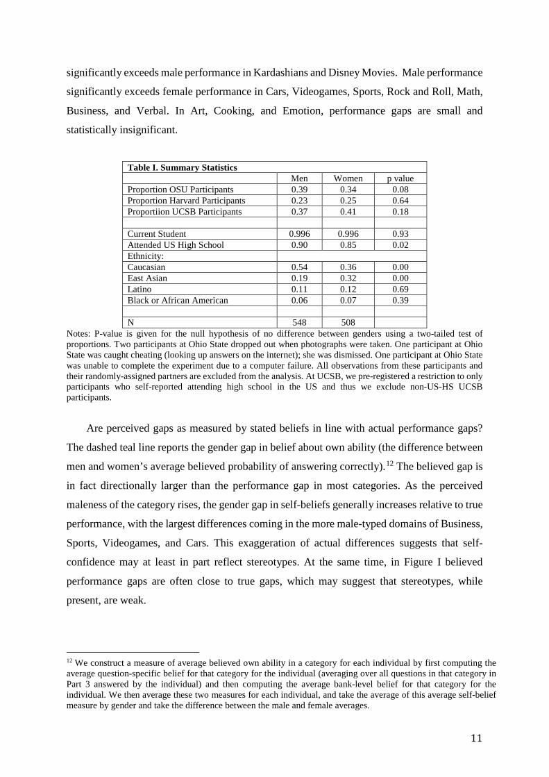
exploring how these measures vary by gender, category, and question difficulty. Table I
presents summary statistics on our participants. In our sample, men are significantly more
likely to have attended a U.S. high school, more likely to be white, and less likely to be East
Asian. Appendix D shows that our results are similar in a more ethnically-balanced sample of
men and women who attended high school in the U.S.
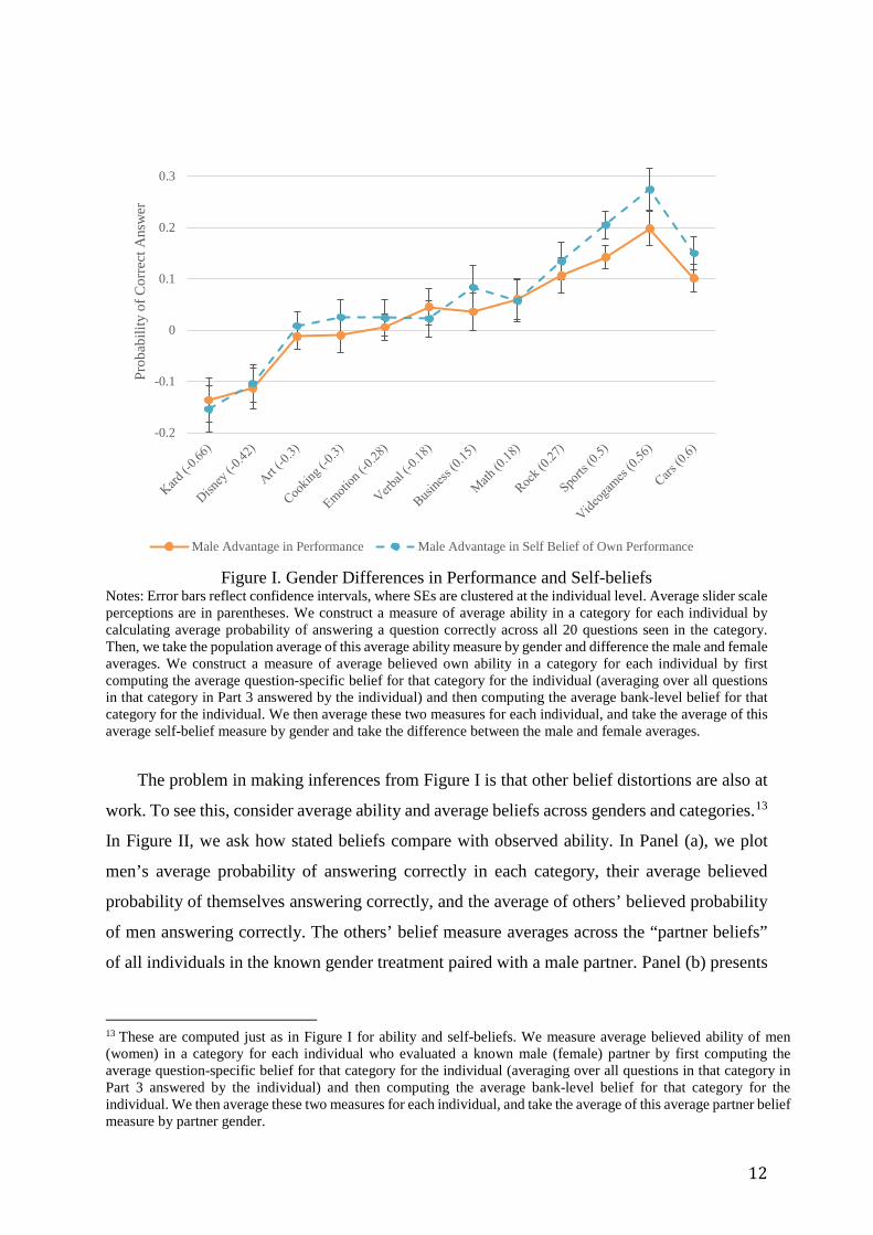
In Figure I, we report actual and believed performance differences between genders. We
have ordered the categories by their average slider scale perception, from most female-typed
to most male-typed. The solid orange line represents the observed male advantage in
performance in each category.11 Categories perceived to be male-typed according to the slider
scale measure tend to also display a male advantage in performance. Female performance
10 We apply the incentive-compatible belief elicitation procedure used by Mobius, Niederle, Niehaus, and Rosenblatt (2014), implemented as in Coffman (2014). At Ohio State, participants see all 40 questions from Part 2 again. For every question they are asked to provide both their believed probability they answered correctly, and their believed probability their partner answered correctly. At Harvard, for 20 of the 40 Part 2 questions, (5 in each category faced by the participant), participants provide their believed probability of answering correctly. For the remaining 20 questions, they provide their believed probability of their partner answering correctly. This is done as a separate section of the experiment. At UCSB, we seek to maximize data collected per participant. We re-present all 120 questions from Parts 1 and 2 (60 for each part). For half the questions, participants provide their own believed probability of answering correctly. For the remaining half of the questions, in a separate block of the experiment, they provide their believed probability of their partner answering correctly. For each mode of belief elicitation, truth-telling is profit-maximizing regardless of the participant’s risk preferences (details in Appendix A). 11 We construct a measure of average ability in a category for each individual by calculating average probability of answering a question correctly across all 20 questions seen in the category. Then, we take the population average of this average ability measure by gender and difference the male and female averages.
11
significantly exceeds male performance in Kardashians and Disney Movies. Male performance
significantly exceeds female performance in Cars, Videogames, Sports, Rock and Roll, Math,
Business, and Verbal. In Art, Cooking, and Emotion, performance gaps are small and
statistically insignificant.
Table I. Summary Statistics Men Women p value Proportion OSU Participants 0.39 0.34 0.08 Proportion Harvard Participants 0.23 0.25 0.64 Proportiion UCSB Participants 0.37 0.41 0.18 Current Student 0.996 0.996 0.93 Attended US High School 0.90 0.85 0.02 Ethnicity: Caucasian 0.54 0.36 0.00 East Asian 0.19 0.32 0.00 Latino 0.11 0.12 0.69 Black or African American 0.06 0.07 0.39 N 548 508
Notes: P-value is given for the null hypothesis of no difference between genders using a two-tailed test of proportions. Two participants at Ohio State dropped out when photographs were taken. One participant at Ohio State was caught cheating (looking up answers on the internet); she was dismissed. One participant at Ohio State was unable to complete the experiment due to a computer failure. All observations from these participants and their randomly-assigned partners are excluded from the analysis. At UCSB, we pre-registered a restriction to only participants who self-reported attending high school in the US and thus we exclude non-US-HS UCSB participants.
Are perceived gaps as measured by stated beliefs in line with actual performance gaps?
The dashed teal line reports the gender gap in belief about own ability (the difference between
men and women’s average believed probability of answering correctly).12 The believed gap is
in fact directionally larger than the performance gap in most categories. As the perceived
maleness of the category rises, the gender gap in self-beliefs generally increases relative to true
performance, with the largest differences coming in the more male-typed domains of Business,
Sports, Videogames, and Cars. This exaggeration of actual differences suggests that self-
confidence may at least in part reflect stereotypes. At the same time, in Figure I believed
performance gaps are often close to true gaps, which may suggest that stereotypes, while
present, are weak.
12 We construct a measure of average believed own ability in a category for each individual by first computing the average question-specific belief for that category for the individual (averaging over all questions in that category in Part 3 answered by the individual) and then computing the average bank-level belief for that category for the individual. We then average these two measures for each individual, and take the average of this average self-belief measure by gender and take the difference between the male and female averages.
12
Figure I. Gender Differences in Performance and Self-beliefs Notes: Error bars reflect confidence intervals, where SEs are clustered at the individual level. Average slider scale perceptions are in parentheses. We construct a measure of average ability in a category for each individual by calculating average probability of answering a question correctly across all 20 questions seen in the category. Then, we take the population average of this average ability measure by gender and difference the male and female averages. We construct a measure of average believed own ability in a category for each individual by first computing the average question-specific belief for that category for the individual (averaging over all questions in that category in Part 3 answered by the individual) and then computing the average bank-level belief for that category for the individual. We then average these two measures for each individual, and take the average of this average self-belief measure by gender and take the difference between the male and female averages.
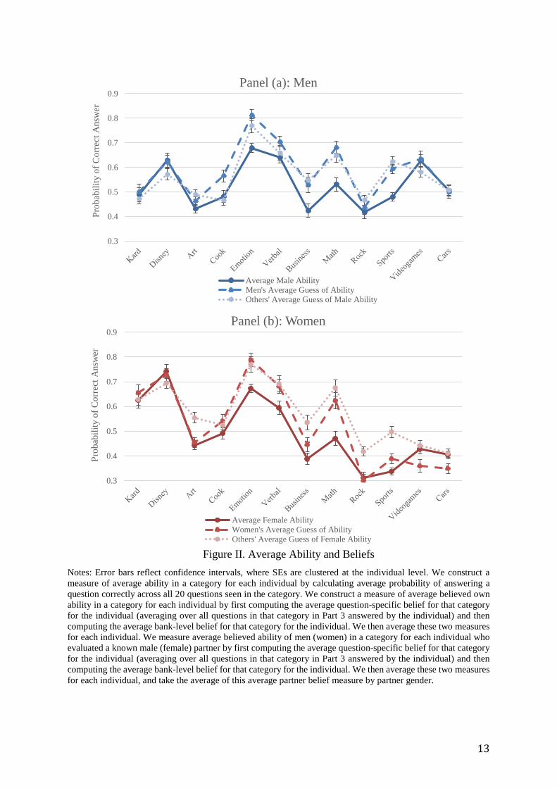
The problem in making inferences from Figure I is that other belief distortions are also at
work. To see this, consider average ability and average beliefs across genders and categories.13
In Figure II, we ask how stated beliefs compare with observed ability. In Panel (a), we plot
men’s average probability of answering correctly in each category, their average believed
probability of themselves answering correctly, and the average of others’ believed probability
of men answering correctly. The others’ belief measure averages across the “partner beliefs”
of all individuals in the known gender treatment paired with a male partner. Panel (b) presents
13 These are computed just as in Figure I for ability and self-beliefs. We measure average believed ability of men (women) in a category for each individual who evaluated a known male (female) partner by first computing the average question-specific belief for that category for the individual (averaging over all questions in that category in Part 3 answered by the individual) and then computing the average bank-level belief for that category for the individual. We then average these two measures for each individual, and take the average of this average partner belief measure by partner gender.
-0.2
-0.1
0
0.1
0.2
0.3
Prob
abili
ty o
f Cor
rect
Ans
wer
Male Advantage in Performance Male Advantage in Self Belief of Own Performance
13
Figure II. Average Ability and Beliefs Notes: Error bars reflect confidence intervals, where SEs are clustered at the individual level. We construct a measure of average ability in a category for each individual by calculating average probability of answering a question correctly across all 20 questions seen in the category. We construct a measure of average believed own ability in a category for each individual by first computing the average question-specific belief for that category for the individual (averaging over all questions in that category in Part 3 answered by the individual) and then computing the average bank-level belief for that category for the individual. We then average these two measures for each individual. We measure average believed ability of men (women) in a category for each individual who evaluated a known male (female) partner by first computing the average question-specific belief for that category for the individual (averaging over all questions in that category in Part 3 answered by the individual) and then computing the average bank-level belief for that category for the individual. We then average these two measures for each individual, and take the average of this average partner belief measure by partner gender.
0.3
0.4
0.5
0.6
0.7
0.8
0.9Pr
obab
ility
of C
orre
ct A
nsw
erPanel (a): Men
Average Male AbilityMen's Average Guess of AbilityOthers' Average Guess of Male Ability
0.3
0.4
0.5
0.6
0.7
0.8
0.9
Prob
abili
ty o
f Cor
rect
Ans
wer
Panel (b): Women
Average Female AbilityWomen's Average Guess of AbilityOthers' Average Guess of Female Ability
14
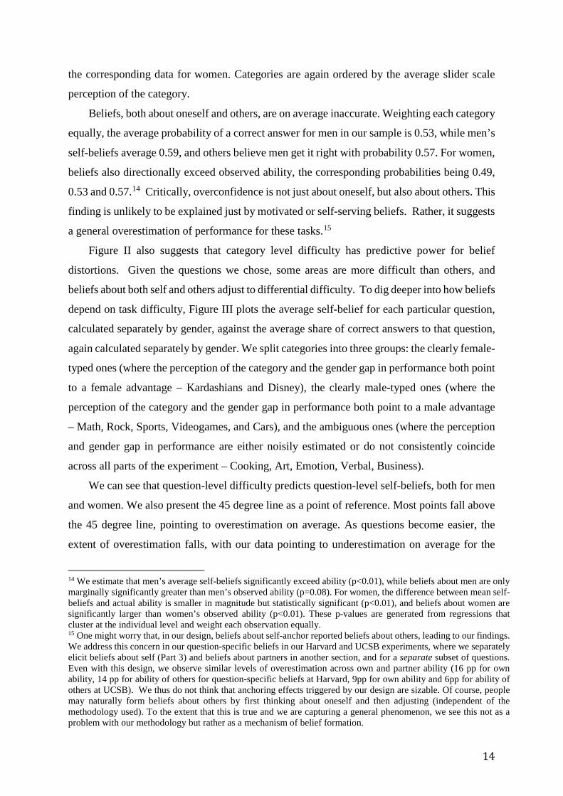
the corresponding data for women. Categories are again ordered by the average slider scale
perception of the category.
Beliefs, both about oneself and others, are on average inaccurate. Weighting each category
equally, the average probability of a correct answer for men in our sample is 0.53, while men’s
self-beliefs average 0.59, and others believe men get it right with probability 0.57. For women,
beliefs also directionally exceed observed ability, the corresponding probabilities being 0.49,
0.53 and 0.57.14 Critically, overconfidence is not just about oneself, but also about others. This
finding is unlikely to be explained just by motivated or self-serving beliefs. Rather, it suggests
a general overestimation of performance for these tasks.15
Figure II also suggests that category level difficulty has predictive power for belief
distortions. Given the questions we chose, some areas are more difficult than others, and
beliefs about both self and others adjust to differential difficulty. To dig deeper into how beliefs
depend on task difficulty, Figure III plots the average self-belief for each particular question,
calculated separately by gender, against the average share of correct answers to that question,
again calculated separately by gender. We split categories into three groups: the clearly female-
typed ones (where the perception of the category and the gender gap in performance both point
to a female advantage – Kardashians and Disney), the clearly male-typed ones (where the
perception of the category and the gender gap in performance both point to a male advantage
– Math, Rock, Sports, Videogames, and Cars), and the ambiguous ones (where the perception
and gender gap in performance are either noisily estimated or do not consistently coincide
across all parts of the experiment – Cooking, Art, Emotion, Verbal, Business).
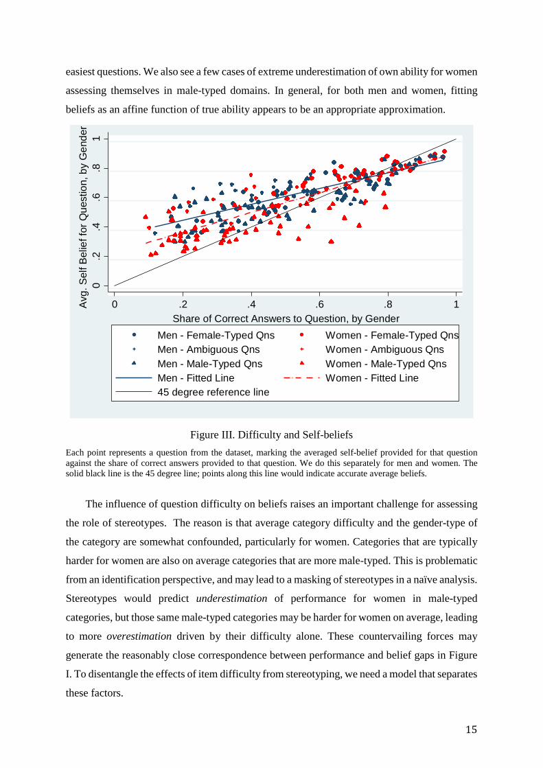
We can see that question-level difficulty predicts question-level self-beliefs, both for men
and women. We also present the 45 degree line as a point of reference. Most points fall above
the 45 degree line, pointing to overestimation on average. As questions become easier, the
extent of overestimation falls, with our data pointing to underestimation on average for the
14 We estimate that men’s average self-beliefs significantly exceed ability (p<0.01), while beliefs about men are only marginally significantly greater than men’s observed ability (p=0.08). For women, the difference between mean self-beliefs and actual ability is smaller in magnitude but statistically significant (p<0.01), and beliefs about women are significantly larger than women’s observed ability (p<0.01). These p-values are generated from regressions that cluster at the individual level and weight each observation equally. 15 One might worry that, in our design, beliefs about self-anchor reported beliefs about others, leading to our findings. We address this concern in our question-specific beliefs in our Harvard and UCSB experiments, where we separately elicit beliefs about self (Part 3) and beliefs about partners in another section, and for a separate subset of questions. Even with this design, we observe similar levels of overestimation across own and partner ability (16 pp for own ability, 14 pp for ability of others for question-specific beliefs at Harvard, 9pp for own ability and 6pp for ability of others at UCSB). We thus do not think that anchoring effects triggered by our design are sizable. Of course, people may naturally form beliefs about others by first thinking about oneself and then adjusting (independent of the methodology used). To the extent that this is true and we are capturing a general phenomenon, we see this not as a problem with our methodology but rather as a mechanism of belief formation.
15
easiest questions. We also see a few cases of extreme underestimation of own ability for women
assessing themselves in male-typed domains. In general, for both men and women, fitting
beliefs as an affine function of true ability appears to be an appropriate approximation.
Figure III. Difficulty and Self-beliefs
Each point represents a question from the dataset, marking the averaged self-belief provided for that question against the share of correct answers provided to that question. We do this separately for men and women. The solid black line is the 45 degree line; points along this line would indicate accurate average beliefs.
The influence of question difficulty on beliefs raises an important challenge for assessing
the role of stereotypes. The reason is that average category difficulty and the gender-type of
the category are somewhat confounded, particularly for women. Categories that are typically
harder for women are also on average categories that are more male-typed. This is problematic
from an identification perspective, and may lead to a masking of stereotypes in a naïve analysis.
Stereotypes would predict underestimation of performance for women in male-typed
categories, but those same male-typed categories may be harder for women on average, leading
to more overestimation driven by their difficulty alone. These countervailing forces may
generate the reasonably close correspondence between performance and belief gaps in Figure
I. To disentangle the effects of item difficulty from stereotyping, we need a model that separates
these factors.
0.2
.4.6
.81
Avg
. Sel
f Bel
ief f
or Q
uest
ion,
by
Gen
der
0 .2 .4 .6 .8 1Share of Correct Answers to Question, by Gender
Men - Female-Typed Qns Women - Female-Typed QnsMen - Ambiguous Qns Women - Ambiguous QnsMen - Male-Typed Qns Women - Male-Typed QnsMen - Fitted Line Women - Fitted Line45 degree reference line
16
4. The Model
There are two groups of participants, 𝐺𝐺 = 𝑀𝑀,𝐹𝐹 (for male and female) and 12 categories
of questions, 𝐽𝐽 ∈{Kardashians, Disney, Art, Cooking, Emotion, Verbal, Business, Math, Rock,
Sports, Cars, Videogames}. Denote by 𝑝𝑝𝑖𝑖,𝑗𝑗 the probability that individual 𝑖𝑖 ∈ 𝐺𝐺 answers the
question 𝑗𝑗 ∈ 𝐽𝐽 correctly. We assume that 𝑝𝑝𝑖𝑖,𝑗𝑗 is given by:
𝑝𝑝𝑖𝑖,𝑗𝑗 = 𝑝𝑝𝐺𝐺,𝐽𝐽 + 𝑎𝑎𝑖𝑖,𝑗𝑗, (1)
where 𝑝𝑝𝐺𝐺,𝐽𝐽 is average performance of gender 𝐺𝐺 in the bank of 10 questions from category 𝐽𝐽
that question j is drawn from. Component 𝑎𝑎𝑖𝑖,𝑗𝑗 captures individual-specific ability and question-
specific difficulty. At the gender-category level, the definition 𝔼𝔼𝑖𝑖𝑗𝑗�𝑝𝑝𝑖𝑖,𝑗𝑗� = 𝑝𝑝𝐺𝐺,𝐽𝐽 imposes
𝔼𝔼𝑖𝑖𝑗𝑗�𝑎𝑎𝑖𝑖,𝑗𝑗� = 0. Individual 𝑖𝑖 ∈ 𝐺𝐺 is better than the average member of group 𝐺𝐺 in category 𝐽𝐽 if
𝔼𝔼𝑗𝑗�𝑎𝑎𝑖𝑖,𝑗𝑗� > 0. Question 𝑗𝑗 ∈ 𝐽𝐽 is easier than the average in category 𝐽𝐽 if 𝔼𝔼𝑖𝑖�𝑎𝑎𝑖𝑖,𝑗𝑗� > 0.
Mis-estimation of Ability and Question Difficulty
In our data, participants systematically overestimate their performance in harder questions.
The cause of this phenomenon is an open question. In a study of overconfidence not focused
on gender, Moore and Healy (MH 2008) attribute it to imperfect information about individual
ability.16 Excess optimism for hard questions may also be due to a mechanical overweighting
of low probability events, possibility related to the probability weighting function of Kahneman
and Tversky’s Prospect Theory (1979). Alternatively, these distortions could be due to over-
precision, or excessive confidence in the accuracy of beliefs (MH 2008). Because our questions
are multiple-choice, an excessive confidence that one’s answer is correct will exactly
overestimate her probability of answering correctly. A fourth possibility is that people
overestimate their performance due to self-serving beliefs about own ability, or image concerns
that motivate them to view themselves favorably. Finally, the larger amount of overestimation
for more difficult questions could be driven by noise in beliefs – if beliefs are random and
constrained to be between 0 and 1, we would also expect more overestimation for the more
difficult questions.
Here we do not seek to distinguish these mechanisms, but call this broad phenomenon
Difficulty Induced Mis-estimation, or DIM. To measure the total role of DIM in the data, and
16 In MH (2008), agents know their average ability in a category, but get a noisy signal of the difficulty of a specific question. Bayesian agents should discount the noisy signal, generating overestimation (underestimation) for questions that are hard (easy) relative to the agents’ expectations. The same mechanism generates similar patterns when assessing others.
17
to separate it from stereotypes, we specify the perceived probability 𝑝𝑝𝑖𝑖,𝑗𝑗𝐷𝐷𝐷𝐷𝐷𝐷 of answering
correctly to be an affine transformation of the true ability 𝑝𝑝𝑖𝑖,𝑗𝑗:
𝑝𝑝𝑖𝑖,𝑗𝑗𝐷𝐷𝐷𝐷𝐷𝐷 = 𝑐𝑐 + 𝜔𝜔𝑝𝑝𝑖𝑖,𝑗𝑗, (2)
where 𝑐𝑐 and 𝜔𝜔 are such that beliefs always lie in [0,1]. This affine approximation appears to
be consistent with the data presented in Figure III. When 𝑐𝑐 > 0 and 𝜔𝜔 ∈ (0,1) participants
overestimate ability in hard questions where 𝑝𝑝𝑖𝑖,𝑗𝑗 is low, and may underestimate it when 𝑝𝑝𝑖𝑖,𝑗𝑗 is
high. Accurate estimation in easy questions occurs if 𝑐𝑐 = 1 − 𝜔𝜔 > 0.
Our belief measures for each participant come from estimation tasks, where participants
are asked to evaluate their absolute ability (either their probability of answering correctly, or
their score on a 10-question bank). We then classify beliefs that on average exceed observed
ability as “overconfidence”. In a critique of the overconfidence literature, Benoit and Dubra
(2011) show that learning from own performance can rationally produce overplacement in
tasks where participants are asked to evaluate themselves relative to others. That is, 𝑦𝑦% of
subjects can rationally believe that they are in the top 𝑥𝑥% of the distribution, with 𝑦𝑦 > 𝑥𝑥. Our
setting is not of this form. Instead, our estimation setting is closer to what Benoit and Dubra
refer to as a “scale experiment”, where beliefs that are too high on average cannot be
rationalized (see Theorem 3 in Benoit Dubra 2011).
Stereotypes
We model stereotypes following BCGS (2016). Consider a decision-maker trying to assess
the distribution of some set of types in a target group, G. These types could be categorical, such
as occupations, hair colors, or political affiliations, or ordered, such as math abilities, heights,
or incomes. In BCGS (2016), when forecasting the distribution of types in some target group
G, the decision-maker compares the target group to a comparison group -G. The model posits
that the decision-maker’s beliefs about the target group are swayed by the representativeness
heuristic (Kahneman and Tversky 1972), the tendency to overestimate the likelihood of types
that are relatively more likely in the target group than in the comparison group.
Take a simple example connected to gender. Suppose a decision maker is trying to assess
the distribution of math abilities among men. The model postulates that the decision maker
compares, perhaps by sampling from memory, the distribution of math abilities among men to
the distribution from a natural comparison group, such as women. The decision maker’s beliefs
about the abilities of men are then shifted toward the more representative types, which are
ability levels that are relatively more frequent among men than women. For instance, if abilities
18
in the two genders are normally distributed with slightly different means, the representative
types occur in the tails. As a result, men may be over-represented in the high-ability tail relative
to women, even if the absolute frequency of these high-ability types is extremely low. In this
case, the decision maker swayed by representativeness would get the direction of the gender
gap right but exaggerate its magnitude. A tiny male advantage in math on average will be
translated into a larger believed advantage.
With this approach, stereotypes contain a “kernel of truth”: they exaggerate true group
differences by focusing on the, often unlikely, features that distinguish one group from the
other. BCGS (2016) show that beliefs about Conservatives and Liberals in the US exhibit such
a kernel of truth: when asked to estimate the average position of a political group on an issue,
participants get the direction of the average difference right, but overestimate its magnitude.17
This overestimation is larger when a party’s extreme types occur with low frequency in
absolute terms, but high relative frequency compared to the other party.
In our setup, stereotypes distort the perceived ability 𝑝𝑝𝐺𝐺,𝐽𝐽 of the average member of a given
gender. In each question within a category 𝐽𝐽, we model each gender as distributed over two
types: “answering correctly” and “answering incorrectly”. Aggregating to the category level,
for gender 𝐺𝐺 (resp. –𝐺𝐺) the probability of these types is 𝑝𝑝𝐺𝐺,𝐽𝐽 and 1 − 𝑝𝑝𝐺𝐺,𝐽𝐽 (resp. 𝑝𝑝−𝐺𝐺,𝐽𝐽 and 1 −
𝑝𝑝−𝐺𝐺,𝐽𝐽). Following BCGS, we say that “answering correctly” is more representative for group
𝐺𝐺 in category 𝐽𝐽 than “answering incorrectly” when 𝑝𝑝𝐺𝐺,𝐽𝐽
𝑝𝑝−𝐺𝐺,𝐽𝐽> 1−𝑝𝑝𝐺𝐺,𝐽𝐽
1−𝑝𝑝−𝐺𝐺,𝐽𝐽, that is, when 𝑝𝑝𝐺𝐺,𝐽𝐽 > 𝑝𝑝−𝐺𝐺,𝐽𝐽.
The stereotypical ability of the average member of 𝐺𝐺 in category 𝐽𝐽 is given by:
𝑝𝑝𝐺𝐺,𝐽𝐽𝑠𝑠𝑠𝑠 = 𝑝𝑝𝐺𝐺,𝐽𝐽 �
𝑝𝑝𝐺𝐺,𝐽𝐽
𝑝𝑝−𝐺𝐺,𝐽𝐽�𝜃𝜃𝜃𝜃 1𝑍𝑍𝐽𝐽,𝐺𝐺
, (3)
where 𝜃𝜃 ≥ 0 is a measure of representativeness-driven distortions and 𝑍𝑍𝐽𝐽,𝐺𝐺 is a normalizing
factor so that 𝑝𝑝𝐺𝐺,𝐽𝐽𝑠𝑠𝑠𝑠 +�1 − 𝑝𝑝𝐺𝐺,𝐽𝐽�
𝑠𝑠𝑠𝑠= 1. Parameter 𝜎𝜎 captures the mental prominence of cross
gender comparisons: the higher is 𝜎𝜎, the more are male-female gender comparisons top of
mind. The case 𝜃𝜃𝜎𝜎 = 0 describes the rational agent. When 𝜃𝜃𝜎𝜎 > 0, representative types are
overweighted. This is different from statistical discrimination, where individuals 𝑖𝑖 ∈ 𝐺𝐺 are
judged as the average member of gender 𝐺𝐺, overweighting 𝑝𝑝𝐺𝐺,𝐽𝐽 relative to 𝑎𝑎𝑖𝑖,𝑗𝑗, but there is no
average distortion in 𝐺𝐺.
17 Other models, including work on naïve realism by Keltner and Robinson (1996), can generate similar exaggeration of differences in political and other contexts. The key distinguishing feature of our approach is its connection to the true distribution of underlying types, and the way representativeness serves to distort beliefs about these distributions.
19
When 𝑝𝑝𝐺𝐺,𝐽𝐽 is close to 𝑝𝑝−𝐺𝐺,𝐽𝐽, Equation (3) can be linearly approximated as18
𝑝𝑝𝐺𝐺,𝐽𝐽𝑠𝑠𝑠𝑠 = 𝑝𝑝𝐺𝐺,𝐽𝐽 + 𝜃𝜃𝜎𝜎�𝑝𝑝𝐺𝐺,𝐽𝐽 − 𝑝𝑝−𝐺𝐺,𝐽𝐽�. (4)
The stereotypical belief of gender 𝐺𝐺 in category 𝐽𝐽 entails an adjustment 𝜃𝜃𝜎𝜎�𝑝𝑝𝐺𝐺,𝐽𝐽 − 𝑝𝑝−𝐺𝐺,𝐽𝐽� in
the direction of the true average gap �𝑝𝑝𝐺𝐺,𝐽𝐽 − 𝑝𝑝−𝐺𝐺,𝐽𝐽� between genders. In domains where men
are on average better than women, 𝑝𝑝𝐷𝐷,𝐽𝐽 > 𝑝𝑝𝐹𝐹,𝐽𝐽, the average ability of men is overestimated and
that of women is underestimated.
The effect of the gender gap in beliefs is stronger when gender comparisons are more top of
mind, namely when 𝜎𝜎 is higher. Although we try to reduce the prominence of gender
comparisons in the experiment, different experimental treatments, in particular the assignment
of a male or female partner, could be expected to influence 𝜎𝜎.
Estimating Equations and Empirical Strategy
Denote by 𝑝𝑝𝑖𝑖,𝑗𝑗𝑏𝑏 the probability that person 𝑖𝑖 believes he or she has correctly answered
question 𝑗𝑗 . We assume that belief 𝑝𝑝𝑖𝑖,𝑗𝑗𝑏𝑏 is distorted by two separate influences: difficulty
induced mis-estimation 𝑝𝑝𝑖𝑖,𝑗𝑗𝐷𝐷𝐷𝐷𝐷𝐷 of true ability and the gender stereotype in category J. Formally,
we write:
𝑝𝑝𝑖𝑖,𝑗𝑗𝑏𝑏 = 𝑐𝑐 + 𝜔𝜔�𝑝𝑝𝐺𝐺,𝐽𝐽 + 𝑎𝑎𝑖𝑖,𝑗𝑗� + 𝜃𝜃𝜎𝜎�𝑝𝑝𝐺𝐺,𝐽𝐽 − 𝑝𝑝−𝐺𝐺,𝐽𝐽�. (5)
This equation nests rational expectation for 𝑐𝑐 = 𝜃𝜃𝜎𝜎 = 0 and 𝜔𝜔 = 1, in which case beliefs only
depend on the objective gender and individual-level abilities. If 𝜃𝜃𝜎𝜎 = 0, but 𝑐𝑐 ≠ 0 or 𝜔𝜔 ≠ 1,
then DIM is the only departure from rational expectations. If instead 𝜃𝜃𝜎𝜎 > 0, but 𝑐𝑐 = 0 and
𝜔𝜔 = 1, distortions are driven only by stereotypes.19
We use Equation (5) to organize our investigation of beliefs both at the question and bank
levels. DIM, characterized by the constant 𝑐𝑐 and slope 𝜔𝜔, can be identified by comparing
beliefs to objective ability either across questions within a given category 𝐽𝐽 or across
individuals with different abilities. This effect is orthogonal to gender stereotypes, which are
identified by comparing beliefs across categories, controlling for question difficulty.
18 To see this, start from 𝑝𝑝𝐺𝐺,𝐽𝐽
𝜃𝜃 = 𝑝𝑝𝐺𝐺 ,𝐽𝐽 �𝑝𝑝𝐺𝐺,𝐽𝐽 + �1 − 𝑝𝑝𝐺𝐺,𝐽𝐽� ∙ �1−𝑝𝑝𝐺𝐺,𝐽𝐽1−𝑝𝑝−𝐺𝐺,𝐽𝐽
�𝜃𝜃∙ � 𝑝𝑝𝐺𝐺,𝐽𝐽
𝑝𝑝−𝐺𝐺,𝐽𝐽�−𝜃𝜃�−1
. Write 𝑝𝑝𝐺𝐺 ,𝐽𝐽 = 𝑝𝑝−𝐺𝐺,𝐽𝐽 + 𝜖𝜖, so that
� 1−𝑝𝑝𝐺𝐺,𝐽𝐽1−𝑝𝑝−𝐺𝐺,𝐽𝐽
�𝜃𝜃
~1 − 𝜃𝜃1−𝑝𝑝−𝐺𝐺,𝐽𝐽
𝜖𝜖 and � 𝑝𝑝𝐺𝐺,𝐽𝐽𝑝𝑝−𝐺𝐺,𝐽𝐽
�−𝜃𝜃
~1 − 𝜃𝜃𝑝𝑝−𝐺𝐺,𝐽𝐽
𝜖𝜖. Then expand 𝑝𝑝𝐺𝐺,𝐽𝐽𝜃𝜃 to first order in 𝜖𝜖 to get the result.
19 Equation (5) can be equivalently derived by assuming that DIM applies to stereotyped beliefs, in the sense that 𝑝𝑝𝑖𝑖,𝑗𝑗𝑏𝑏 = 𝑐𝑐 + 𝜔𝜔�𝑝𝑝𝐺𝐺,𝐽𝐽
𝑠𝑠𝑠𝑠 + 𝑎𝑎𝑖𝑖,𝑗𝑗� . In this case, the coefficient in front of the gender gap is 𝜔𝜔𝜃𝜃𝜎𝜎 and not 𝜃𝜃𝜎𝜎.
20
We next present our estimating equations along these dimensions and discuss econometric
issues. We have two ways of estimating the roles of DIM and stereotypes. First, and most
directly, we can estimate Equation (5) using beliefs about own performance at the question
level. This estimation uses the question-level beliefs data from Part 3 of the experiment. This
approach identifies DIM from variation in question-level difficulty within categories, holding
the category-level stereotype constant.
The second approach is to use assessments at the category level, with the bank-level beliefs
about own score on the 10-question bank provided following Part 1 (and Part 2 for UCSB
participants). Using Equation (5), the belief about own performance at the category level (Part
1 or 2) is:
𝔼𝔼𝑗𝑗∈𝐽𝐽�𝑝𝑝𝑖𝑖,𝑗𝑗𝑏𝑏 � = 𝑐𝑐 + 𝜔𝜔 �𝑝𝑝𝐺𝐺,𝐽𝐽 + 𝔼𝔼𝑗𝑗∈𝐽𝐽�𝑎𝑎𝑖𝑖,𝑗𝑗�� + 𝜃𝜃𝜎𝜎�𝑝𝑝𝐺𝐺,𝐽𝐽 − 𝑝𝑝−𝐺𝐺,𝐽𝐽�, (6)
where 𝔼𝔼𝑗𝑗∈𝐽𝐽�𝑝𝑝𝑖𝑖,𝑗𝑗𝑏𝑏 � is the average probability of answering correctly a question in category 𝐽𝐽. In
Equation (6), the DIM parameters 𝑐𝑐 and 𝜔𝜔 are estimated using variation across individuals
with different abilities, not across specific questions within an individual as in the question-
level estimation. Thus, Equations (5) and (6) use different sources of variation to estimate DIM,
allowing us to assess robustness of our results.
We next consider beliefs about others. We focus on participants who knew the gender of
their partner. The belief 𝑝𝑝𝑖𝑖′→𝑖𝑖,𝑗𝑗𝑏𝑏 held by individual 𝑖𝑖′ about the performance of individual 𝑖𝑖 ∈ 𝐺𝐺
on a given question 𝑗𝑗 (Part 3) is:
𝑝𝑝𝑖𝑖′→𝑖𝑖,𝑗𝑗𝑏𝑏 = 𝑐𝑐 + 𝜔𝜔 �𝑝𝑝𝐺𝐺,𝐽𝐽 + 𝔼𝔼𝑖𝑖�𝑎𝑎𝑖𝑖,𝑗𝑗�� + 𝜃𝜃𝜎𝜎�𝑝𝑝𝐺𝐺,𝐽𝐽 − 𝑝𝑝−𝐺𝐺,𝐽𝐽�. (7)
The term 𝔼𝔼𝑖𝑖�𝑎𝑎𝑖𝑖,𝑗𝑗� reflects the fact that 𝑖𝑖′ has no specific information about the ability of 𝑖𝑖 in
question j, so beliefs should depend on the average hit rate of gender 𝐺𝐺 for the same question.
The average believed score out of 10 for a generic member of 𝐺𝐺 in category 𝐽𝐽 satisfies:
𝔼𝔼𝑗𝑗∈𝐽𝐽�𝑝𝑝𝑖𝑖′→𝑖𝑖,𝑗𝑗𝑏𝑏 � = 𝑐𝑐 + 𝜔𝜔𝑝𝑝𝐺𝐺,𝐽𝐽 + 𝜃𝜃𝜎𝜎�𝑝𝑝𝐺𝐺,𝐽𝐽 − 𝑝𝑝−𝐺𝐺,𝐽𝐽�. (8)
Equations (7, 8) allow us to estimate beliefs about the performance of each gender using
question-level and bank-level data, respectively.
We follow a common empirical strategy and estimate Equations (5-8) separately for men
and women and separately for beliefs about self and others. Allowing parameters 𝑐𝑐,𝜔𝜔, and 𝜃𝜃𝜎𝜎
to vary across genders and belief types can be informative. For instance, this approach can
detect differences in DIM between men and women or in beliefs about self and others (e.g.,
self-serving overconfidence should only affect self-beliefs). The stereotypes coefficient 𝜃𝜃𝜎𝜎
may be higher if gender comparisons become top of mind when the partner is revealed to be
21
of the opposite gender, or when beliefs are elicited about performance in a category as opposed
to a specific question.
Two main econometric issues arise when bringing specifications (5) through (8) to the
data. Estimation relies on finding proxies for: i) the gender gap �𝑝𝑝𝐺𝐺,𝐽𝐽 − 𝑝𝑝−𝐺𝐺,𝐽𝐽� in performance
and ii) individual as well as group level ability. We next discuss how we handle these
explanatory variables, starting with the gender gap.
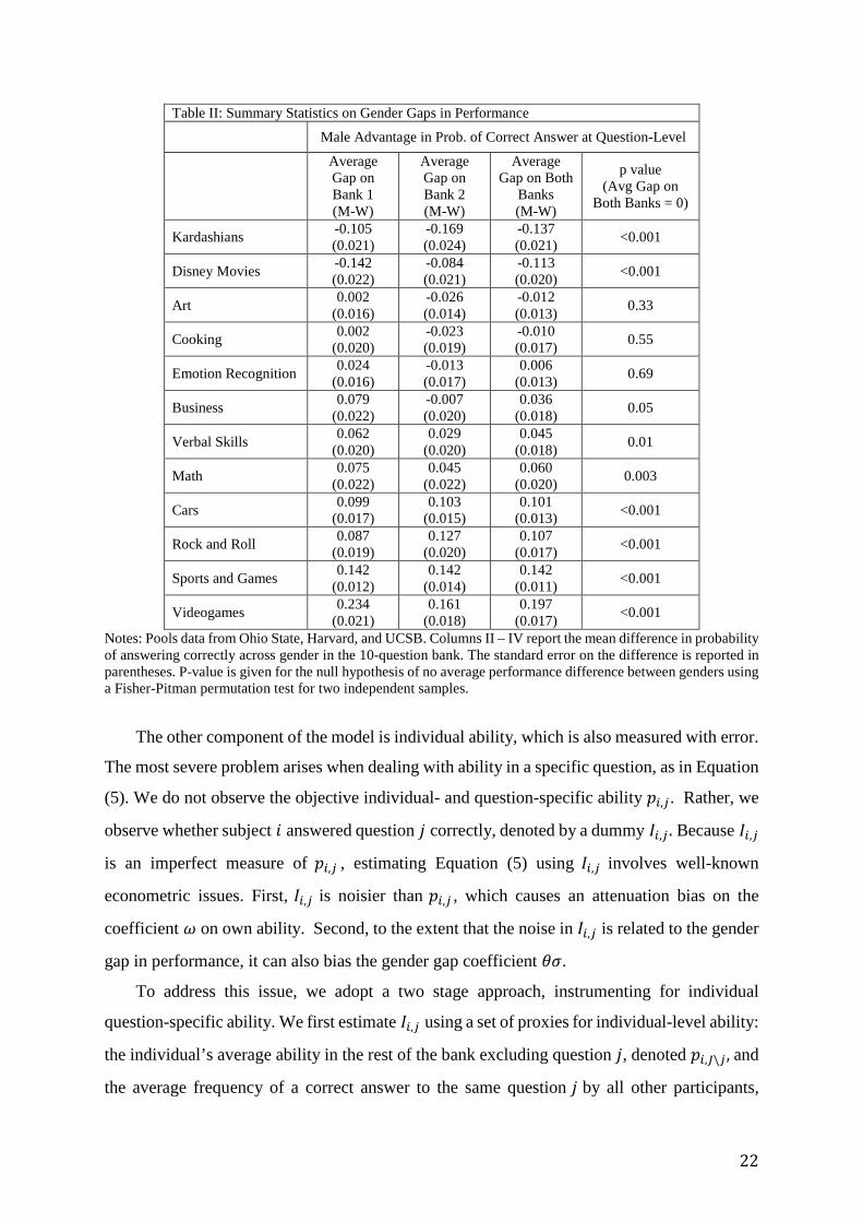
Consider the gender gap in performance in category 𝐽𝐽. Because 𝔼𝔼𝑖𝑖∈𝐺𝐺,𝑗𝑗∈𝐽𝐽�𝑎𝑎𝑖𝑖,𝑗𝑗� = 0, a proxy
for the gap �𝑝𝑝𝐺𝐺,𝐽𝐽 − 𝑝𝑝−𝐺𝐺,𝐽𝐽� in the data is given by the average performance gap between genders
in the bank of 10 questions in category J. With sufficiently large N, this measure should be
reliable. Table II reports these performance gaps measured as the difference in the probability
of answering a question correctly, separated by gender and category, for the two 10-question
banks in each category. Men outperform women significantly in Math, Cars, Rock, Sports, and
Videogames in both banks while women outperform men significantly in Kardashians and
Disney. Gaps in the other categories are mixed. In Business and Verbal Skills, men outperform
women by a significant margin in bank 1, but not in bank 2. In the other stereotypically female
categories (Emotion, Art, and Cooking), performance gaps are small and statistically
insignificant.20
This evidence raises two issues. First, observed gender gaps in some categories are small
and noisily estimated, which introduces noise in our estimation of 𝜃𝜃. Second, and related,
stereotypes may be formed on the basis of gender gaps observed outside of our lab experiment
– e.g. the gender gap in the broader population – which would also affect estimates of 𝜃𝜃. To
address these concerns, we perform two robustness checks. First, we replace observed gaps
with the slider scale perceptions provided by participants, which proxy for gender gaps in the
broader population (Section 5.4). Second, we restrict attention to categories in which the gender
gaps are large and stable across different measurements (see Appendix D). Both of these tests
suggest, if anything, a marginally stronger average impact of stereotypes on beliefs. The fact
that estimates of 𝜃𝜃 remain fairly stable for these various specifications suggests that imperfect
measurement of the relevant gender gap does not pose a substantial threat to our analysis.
20 Our math questions are taken from a practice test for the GMAT Exam. In 2012 – 2013, the gender gap in mean GMAT scores in the United States was 549 vs. 504 (out of 800). See: http://www.gmac.com/~/media/Files/gmac/Research/GMAT%20Test%20Taker%20Data/2013-gmat-profile-exec-summary.pdf. Our verbal questions are taken from practice tests for the Verbal Reasoning and Writing sections of the SAT I. The relative performances we observe are broadly in line with other evidence. In SAT exams, taken by a population in many ways similar to our lab sample, men perform better than women in math (527 vs 496 out of 800) and perform equally in verbal questions (critical reading plus writing, 488 vs 492 out of 800), though these differences are not significant.
22
Table II: Summary Statistics on Gender Gaps in Performance Male Advantage in Prob. of Correct Answer at Question-Level
Average Gap on Bank 1 (M-W)
Average Gap on Bank 2 (M-W)
Average Gap on Both
Banks (M-W)
p value (Avg Gap on
Both Banks = 0)
Kardashians -0.105 (0.021)
-0.169 (0.024)
-0.137 (0.021) <0.001
Disney Movies -0.142 (0.022)
-0.084 (0.021)
-0.113 (0.020) <0.001
Art 0.002 (0.016)
-0.026 (0.014)
-0.012 (0.013) 0.33
Cooking 0.002 (0.020)
-0.023 (0.019)
-0.010 (0.017) 0.55
Emotion Recognition 0.024 (0.016)
-0.013 (0.017)
0.006 (0.013) 0.69
Business 0.079 (0.022)
-0.007 (0.020)
0.036 (0.018) 0.05
Verbal Skills 0.062 (0.020)
0.029 (0.020)
0.045 (0.018) 0.01
Math 0.075 (0.022)
0.045 (0.022)
0.060 (0.020) 0.003
Cars 0.099 (0.017)
0.103 (0.015)
0.101 (0.013) <0.001
Rock and Roll 0.087 (0.019)
0.127 (0.020)
0.107 (0.017) <0.001
Sports and Games 0.142 (0.012)
0.142 (0.014)
0.142 (0.011) <0.001
Videogames 0.234 (0.021)
0.161 (0.018)
0.197 (0.017) <0.001
Notes: Pools data from Ohio State, Harvard, and UCSB. Columns II – IV report the mean difference in probability of answering correctly across gender in the 10-question bank. The standard error on the difference is reported in parentheses. P-value is given for the null hypothesis of no average performance difference between genders using a Fisher-Pitman permutation test for two independent samples.
The other component of the model is individual ability, which is also measured with error.
The most severe problem arises when dealing with ability in a specific question, as in Equation
(5). We do not observe the objective individual- and question-specific ability 𝑝𝑝𝑖𝑖,𝑗𝑗. Rather, we
observe whether subject 𝑖𝑖 answered question 𝑗𝑗 correctly, denoted by a dummy 𝐼𝐼𝑖𝑖,𝑗𝑗 . Because 𝐼𝐼𝑖𝑖,𝑗𝑗
is an imperfect measure of 𝑝𝑝𝑖𝑖,𝑗𝑗 , estimating Equation (5) using 𝐼𝐼𝑖𝑖,𝑗𝑗 involves well-known
econometric issues. First, 𝐼𝐼𝑖𝑖,𝑗𝑗 is noisier than 𝑝𝑝𝑖𝑖,𝑗𝑗 , which causes an attenuation bias on the
coefficient 𝜔𝜔 on own ability. Second, to the extent that the noise in 𝐼𝐼𝑖𝑖,𝑗𝑗 is related to the gender
gap in performance, it can also bias the gender gap coefficient 𝜃𝜃𝜎𝜎.
To address this issue, we adopt a two stage approach, instrumenting for individual
question-specific ability. We first estimate 𝐼𝐼𝑖𝑖,𝑗𝑗 using a set of proxies for individual-level ability:
the individual’s average ability in the rest of the bank excluding question 𝑗𝑗, denoted 𝑝𝑝𝑖𝑖,𝐽𝐽\𝑗𝑗, and
the average frequency of a correct answer to the same question 𝑗𝑗 by all other participants,
23
𝑝𝑝𝐺𝐺∪−𝐺𝐺\𝑖𝑖,𝑗𝑗 . 21 These proxies do not use information about participant 𝑖𝑖 ’s performance on
question 𝑗𝑗, but still capture her ability in the category 𝐽𝐽 and the question’s overall difficulty.
We implement the first stage regression:
𝐼𝐼𝑖𝑖,𝑗𝑗 = 𝛼𝛼0 + 𝛼𝛼1 𝑝𝑝𝑖𝑖,𝐽𝐽\𝑗𝑗 + 𝛼𝛼2𝑝𝑝𝐺𝐺∪−𝐺𝐺\𝑖𝑖,𝑗𝑗 + 𝛼𝛼3�𝑝𝑝𝐺𝐺,𝐽𝐽 − 𝑝𝑝−𝐺𝐺,𝐽𝐽� (9)
where the gender gap 𝑝𝑝𝐺𝐺,𝐽𝐽 − 𝑝𝑝−𝐺𝐺,𝐽𝐽 is also included as a regressor. The fitted values 𝐼𝐼𝑖𝑖,𝑗𝑗 of the
above regressions are then used as proxies for true individual- and question-specific ability
𝑝𝑝𝑖𝑖,𝑗𝑗. Instrumenting helps us reduce biases due to noisy ability measurement while preserving
the interpretation of coefficients as distortions due to stereotypes or DIM.22
Finally, ability at the category level, necessary to estimate Equations (6), (7) and (8), is
proxied for with its sample counterpart. Thus �𝑝𝑝𝐺𝐺,𝐽𝐽 + 𝔼𝔼𝑗𝑗∈𝐽𝐽�𝑎𝑎𝑖𝑖,𝑗𝑗�� in Equation (6) is proxied by
the share of correct answers obtained by individual 𝑖𝑖 in category 𝐽𝐽 . Similarly, the ability
measures in Equations (7) and (8) are proxied by the share of correct answers by gender 𝐺𝐺 in
question 𝑗𝑗 and in category 𝐽𝐽, respectively.
5. Determinants of Beliefs
5.1 Beliefs about own performance
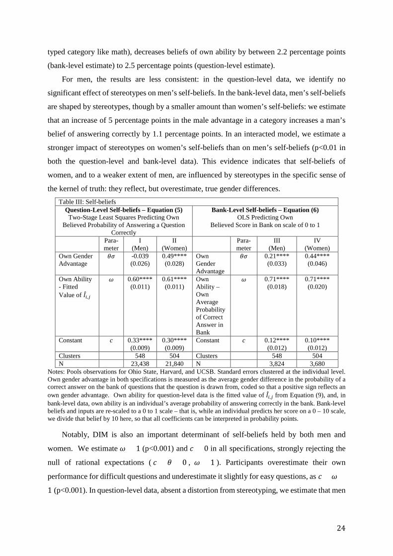
Table III reports the results from specifications (5) and (6) on self-beliefs. Columns I and
II use Part 3 question-level data to estimate Equation (5). We capture ability using the fitted
values 𝐼𝐼𝑖𝑖,𝑗𝑗 described above; first stage estimates appear in Appendix C. Columns III and IV
present the estimates of Equation (6) using bank-level beliefs. To interpret the coefficients in
probability points, we rescale bank-level beliefs (and all inputs) to a probability scale by
dividing by 10.
In three of the four specifications, we identify a significant role for stereotypes in shaping
beliefs about self. For women, the effects are consistent. Specifications II and IV both suggest
that, holding own true ability fixed, a 5 percentage point increase in male advantage in a
category (roughly the size of moving from a gender-neutral category to a moderately male-
21 Alternatively, one could use the share of correct answers to question j by only participants of the same gender, 𝑝𝑝𝐺𝐺\𝑖𝑖,𝑗𝑗. The results of Table III are robust to this alternative specification. 22 In Appendix C, we perform a robustness check of the two-stage approach described above. We separately add the proxies for individual ability, 𝑝𝑝𝑖𝑖,𝐽𝐽\𝑗𝑗 and 𝑝𝑝𝐺𝐺∪−𝐺𝐺\𝑖𝑖,𝑗𝑗 to Equation (5). This provides a simpler method to pinning down the effect of stereotypes; however, we lose the interpretation of 𝑐𝑐 and 𝜔𝜔. Estimated coefficients 𝜃𝜃𝜎𝜎 on the gender gaps are very similar to the two-stage estimates.
24
typed category like math), decreases beliefs of own ability by between 2.2 percentage points
(bank-level estimate) to 2.5 percentage points (question-level estimate).
For men, the results are less consistent: in the question-level data, we identify no
significant effect of stereotypes on men’s self-beliefs. In the bank-level data, men’s self-beliefs
are shaped by stereotypes, though by a smaller amount than women’s self-beliefs: we estimate
that an increase of 5 percentage points in the male advantage in a category increases a man’s
belief of answering correctly by 1.1 percentage points. In an interacted model, we estimate a
stronger impact of stereotypes on women’s self-beliefs than on men’s self-beliefs (p<0.01 in
both the question-level and bank-level data). This evidence indicates that self-beliefs of
women, and to a weaker extent of men, are influenced by stereotypes in the specific sense of
the kernel of truth: they reflect, but overestimate, true gender differences. Table III: Self-beliefs
Question-Level Self-beliefs – Equation (5) Two-Stage Least Squares Predicting Own
Believed Probability of Answering a Question Correctly
Bank-Level Self-beliefs – Equation (6) OLS Predicting Own
Believed Score in Bank on scale of 0 to 1
Para-meter
I (Men)
II (Women)
Para-meter
III (Men)
IV (Women)
Own Gender Advantage
𝜃𝜃𝜎𝜎 -0.039 (0.026)
0.49**** (0.028)
Own Gender Advantage
𝜃𝜃𝜎𝜎 0.21**** (0.033)
0.44**** (0.046)
Own Ability - Fitted Value of 𝐼𝐼𝑖𝑖,𝑗𝑗
𝜔𝜔 0.60**** (0.011)
0.61**** (0.011)
Own Ability –Own Average Probability of Correct Answer in Bank
𝜔𝜔 0.71**** (0.018)
0.71**** (0.020)
Constant c 0.33**** (0.009)
0.30**** (0.009)
Constant c 0.12**** (0.012)
0.10**** (0.012)
Clusters 548 504 Clusters 548 504 N 23,438 21,840 N 3,824 3,680
Notes: Pools observations for Ohio State, Harvard, and UCSB. Standard errors clustered at the individual level. Own gender advantage in both specifications is measured as the average gender difference in the probability of a correct answer on the bank of questions that the question is drawn from, coded so that a positive sign reflects an own gender advantage. Own ability for question-level data is the fitted value of 𝐼𝐼𝑖𝑖,𝑗𝑗 from Equation (9), and, in bank-level data, own ability is an individual’s average probability of answering correctly in the bank. Bank-level beliefs and inputs are re-scaled to a 0 to 1 scale – that is, while an individual predicts her score on a 0 – 10 scale, we divide that belief by 10 here, so that all coefficients can be interpreted in probability points.
Notably, DIM is also an important determinant of self-beliefs held by both men and
women. We estimate 𝜔𝜔 < 1 (p<0.001) and 𝑐𝑐 > 0 in all specifications, strongly rejecting the
null of rational expectations ( 𝑐𝑐 = 𝜃𝜃 = 0 , 𝜔𝜔 = 1 ). Participants overestimate their own
performance for difficult questions and underestimate it slightly for easy questions, as 𝑐𝑐 + 𝜔𝜔 <
1 (p<0.001). In question-level data, absent a distortion from stereotyping, we estimate that men
25
overestimate own performance for questions where own ability is less than or equal to 0.83,
and women overestimate own performance for questions where own ability is less than 0.77.
DIM distortions are smaller in bank-level than in question-level beliefs (𝑐𝑐 is lower and 𝜔𝜔 is
higher in Columns III and IV than in Columns I and II).23
When we compare genders, running an interacted model, we estimate a somewhat smaller
c for women than for men (p<0.01 in the question-level data, n.s. in the bank-level data), but
no significant differences in 𝜔𝜔. Thus, no clear gender differences in DIM emerge in our data
on self-beliefs. While it is difficult to compare this result directly with the earlier work that has
not separated DIM from other sources of belief distortions, such as stereotypes, the null finding
is consistent with the evidence of limited gender differences in overconfidence in neutral-typed
categories. In our data, significant gender differences occur in categories with sizable gender
gaps due to stereotypes.
5.2 Beliefs about others’ performance
Table IV reports estimates of Equations (7) and (8) for beliefs about others’ performance
on individual questions (Columns I and II) and at the bank-level (Columns III and IV). We use
data from participants who knew their partner’s gender, and we pool all evaluators, without
keeping track of their gender. In Appendix C we show effects separately by gender of the
evaluator, finding no consistent differences in how men and women evaluate others.
There are many similarities between Table IV estimates and the self-beliefs estimates of
Table III. Just as in the self-beliefs data, we estimate a significant role for stereotypes in three
out of the four specifications. When evaluating women, stereotypes play a consistent and non-
trivial role in shaping beliefs. Just as increases in male advantage decrease women’s beliefs of
own ability, increases in male advantage also decrease others’ beliefs of women’s ability. This
effect is of roughly the same magnitude in the question-level data: a 5pp increase in male
advantage decreases beliefs of female ability by 2.4pp. In the bank-level beliefs, the effects
are smaller than the effects for self-beliefs, but still significant: an increase in male advantage
of 5pp is estimated to decrease beliefs of female ability by 0.7 pp. The evidence on the role of
stereotypes for beliefs about men is mixed, just as it was for self-beliefs. In the bank-level
data, stereotypes are quite strong, shaping beliefs about men as predicted by the model, just as
they did for self-beliefs. In question-level data, we estimate no significant effect.
23 This is consistent with the Moore and Healy mechanism (subjects perceive a more precise signal of average difficulty after observing 10 questions than after observing a single question) and with overestimation of small probabilities (which exerts a smaller distortion on the average score from several questions).
26
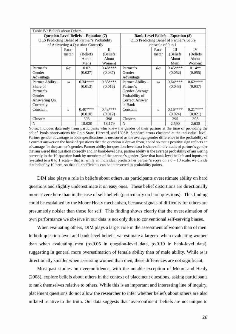
Table IV: Beliefs about Others Question-Level Beliefs – Equation (7)
OLS Predicting Belief of Partner’s Probability of Answering a Question Correctly
Bank-Level Beliefs – Equation (8) OLS Predicting Belief of Partner’s Score
on scale of 0 to 1 Para-
meter I
(Beliefs About Men)
II (Beliefs About
Women)
Para-meter
III (Beliefs About Men)
IV (Beliefs About
Women) Partner’s Gender Advantage
𝜃𝜃𝜎𝜎 0.02 (0.027)
0.48**** (0.037)
Partner’s Gender Advantage
𝜃𝜃𝜎𝜎 0.45**** (0.052)
0.14** (0.055)
Partner Ability - Share of Partner’s Gender Answering Qn. Correctly
𝜔𝜔 0.34**** (0.013)
0.33**** (0.016)
Partner Ability - Partner’s Gender Average Probability of Correct Answer in Bank
𝜔𝜔 0.64**** (0.043)
0.62**** (0.037)
Constant c 0.40**** (0.010)
0.43**** (0.012)
Constant c 0.16**** (0.024)
0.21**** (0.021)
Clusters 395 398 Clusters 395 398 N 18,020 18,179 N 2,590 2,630
Notes: Includes data only from participants who knew the gender of their partner at the time of providing the belief. Pools observations for Ohio State, Harvard, and UCSB. Standard errors clustered at the individual level. Partner gender advantage in both specifications is measured as the average gender difference in the probability of a correct answer on the bank of questions that the question is drawn from, coded so that a positive sign reflects an advantage for the partner’s gender. Partner ability for question-level data is share of individuals of partner’s gender that answered that question correctly and, in bank-level data, partner ability is the average probability of answering correctly in the 10-question bank by members of the partner’s gender. Note that bank-level beliefs and inputs are re-scaled to a 0 to 1 scale – that is, while an individual predicts her partner’s score on a 0 – 10 scale, we divide that belief by 10 here, so that all coefficients can be interpreted in probability points.
DIM also plays a role in beliefs about others, as participants overestimate ability on hard
questions and slightly underestimate it on easy ones. These belief distortions are directionally
more severe here than in the case of self-beliefs (particularly on hard questions). This finding
could be explained by the Moore Healy mechanism, because signals of difficulty for others are
presumably noisier than those for self. This finding shows clearly that the overestimation of
own performance we observe in our data is not only due to conventional self-serving biases.
When evaluating others, DIM plays a larger role in the assessment of women than of men.
In both question-level and bank-level beliefs, we estimate a larger c when evaluating women
than when evaluating men (p<0.05 in question-level data, p<0.10 in bank-level data),
suggesting in general more overestimation of female ability than of male ability. While 𝜔𝜔 is
directionally smaller when assessing women than men, these differences are not significant.
Most past studies on overconfidence, with the notable exception of Moore and Healy
(2008), explore beliefs about others in the context of placement questions, asking participants
to rank themselves relative to others. While this is an important and interesting line of inquiry,
placement questions do not allow the researcher to infer whether beliefs about others are also
inflated relative to the truth. Our data suggests that ‘overconfident’ beliefs are not unique to
27
self-assessments. Note that this is not necessarily inconsistent with past evidence on over-
placement, as beliefs about self could still exceed beliefs about others, even if both are inflated
relative to the truth. We explore the connection between beliefs about absolute and relative
ability in Section 6.
5.3 Taking Stock of Stereotypes and DIM
What do our model and data have to say about gender gaps in confidence? We can use our
estimates to shed light on this question. As a metric for this assessment, we propose the male
overconfidence gap, or MOG, defined as the difference between male and female
overconfidence: MOG = [(Average Male Self-belief – Average Male Ability) – (Average
Female Self-belief – Average Female Ability)]. This measure increases as men become more
overconfident (or less underconfident) about themselves relative to women. In line with our
initial motivation, this measure captures the extent to which self-assessments of confidence
tend to favor men over women relative to real ability.
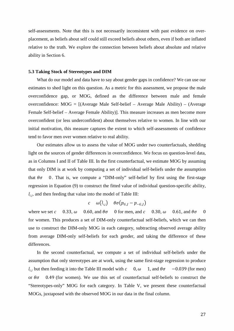
Our estimates allow us to assess the value of MOG under two counterfactuals, shedding
light on the sources of gender differences in overconfidence. We focus on question-level data,
as in Columns I and II of Table III. In the first counterfactual, we estimate MOG by assuming
that only DIM is at work by computing a set of individual self-beliefs under the assumption
that 𝜃𝜃𝜎𝜎 = 0 . That is, we compute a “DIM-only” self-belief by first using the first-stage
regression in Equation (9) to construct the fitted value of individual question-specific ability,
𝐼𝐼𝑖𝑖,𝑗𝑗, and then feeding that value into the model of Table III:
𝑐𝑐 + 𝜔𝜔��̂�𝐼𝑖𝑖,𝑗𝑗� + 𝜃𝜃𝜎𝜎�𝑝𝑝𝐺𝐺,𝐽𝐽 − 𝑝𝑝−𝐺𝐺,𝐽𝐽�
where we set 𝑐𝑐 = 0.33, 𝜔𝜔 = 0.60, and 𝜃𝜃𝜎𝜎 = 0 for men, and 𝑐𝑐 = 0.30, 𝜔𝜔 = 0.61, and 𝜃𝜃𝜎𝜎 = 0
for women. This produces a set of DIM-only counterfactual self-beliefs, which we can then
use to construct the DIM-only MOG in each category, subtracting observed average ability
from average DIM-only self-beliefs for each gender, and taking the difference of these
differences.
In the second counterfactual, we compute a set of individual self-beliefs under the
assumption that only stereotypes are at work, using the same first-stage regression to produce
𝐼𝐼𝑖𝑖,𝑗𝑗 but then feeding it into the Table III model with 𝑐𝑐 = 0,𝜔𝜔 = 1, and 𝜃𝜃𝜎𝜎 = −0.039 (for men)
or 𝜃𝜃𝜎𝜎 = 0.49 (for women). We use this set of counterfactual self-beliefs to construct the
“Stereotypes-only” MOG for each category. In Table V, we present these counterfactual
MOGs, juxtaposed with the observed MOG in our data in the final column.
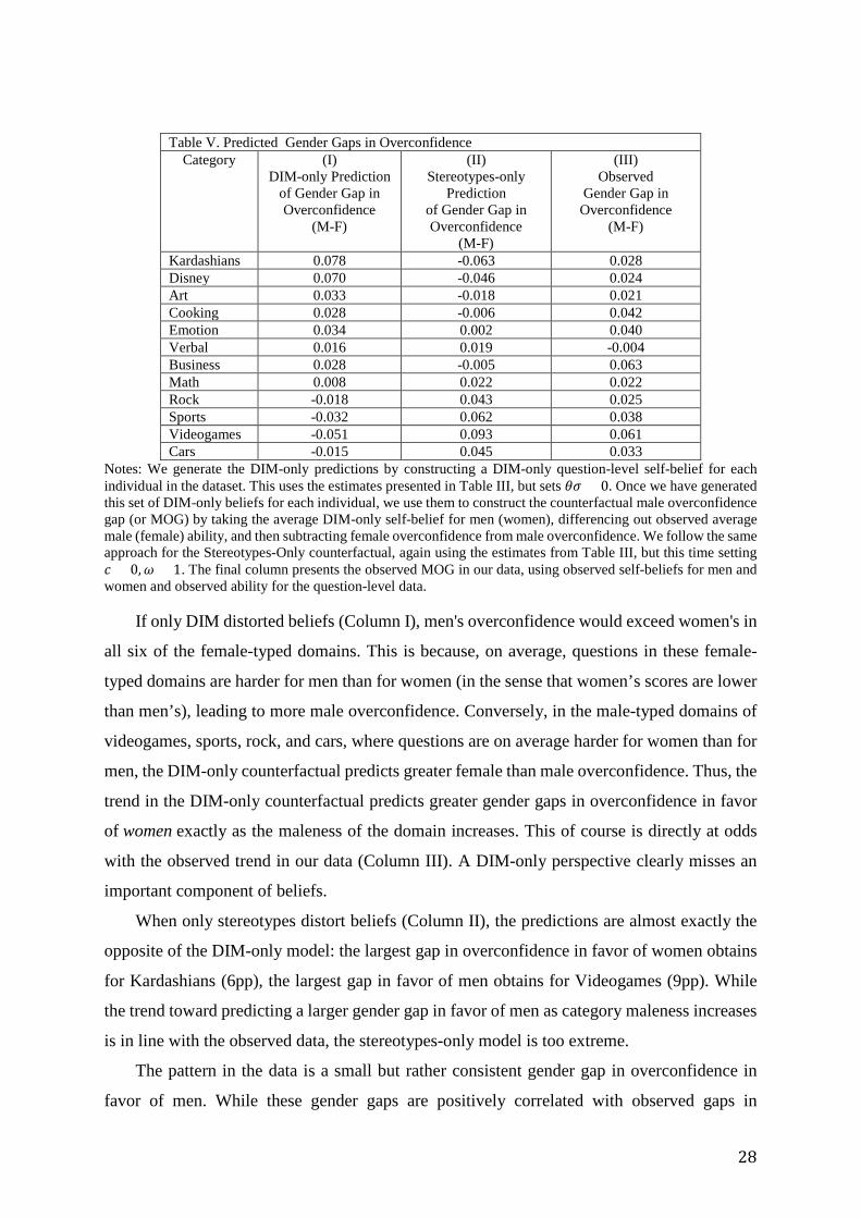
28
Table V. Predicted Gender Gaps in Overconfidence
Category (I) DIM-only Prediction
of Gender Gap in Overconfidence
(M-F)
(II) Stereotypes-only
Prediction of Gender Gap in Overconfidence
(M-F)
(III) Observed
Gender Gap in Overconfidence
(M-F)
Kardashians 0.078 -0.063 0.028 Disney 0.070 -0.046 0.024 Art 0.033 -0.018 0.021 Cooking 0.028 -0.006 0.042 Emotion 0.034 0.002 0.040 Verbal 0.016 0.019 -0.004 Business 0.028 -0.005 0.063 Math 0.008 0.022 0.022 Rock -0.018 0.043 0.025 Sports -0.032 0.062 0.038 Videogames -0.051 0.093 0.061 Cars -0.015 0.045 0.033
Notes: We generate the DIM-only predictions by constructing a DIM-only question-level self-belief for each individual in the dataset. This uses the estimates presented in Table III, but sets 𝜃𝜃𝜎𝜎 = 0. Once we have generated this set of DIM-only beliefs for each individual, we use them to construct the counterfactual male overconfidence gap (or MOG) by taking the average DIM-only self-belief for men (women), differencing out observed average male (female) ability, and then subtracting female overconfidence from male overconfidence. We follow the same approach for the Stereotypes-Only counterfactual, again using the estimates from Table III, but this time setting 𝑐𝑐 = 0,𝜔𝜔 = 1. The final column presents the observed MOG in our data, using observed self-beliefs for men and women and observed ability for the question-level data.
If only DIM distorted beliefs (Column I), men's overconfidence would exceed women's in
all six of the female-typed domains. This is because, on average, questions in these female-
typed domains are harder for men than for women (in the sense that women’s scores are lower
than men’s), leading to more male overconfidence. Conversely, in the male-typed domains of
videogames, sports, rock, and cars, where questions are on average harder for women than for
men, the DIM-only counterfactual predicts greater female than male overconfidence. Thus, the
trend in the DIM-only counterfactual predicts greater gender gaps in overconfidence in favor
of women exactly as the maleness of the domain increases. This of course is directly at odds
with the observed trend in our data (Column III). A DIM-only perspective clearly misses an
important component of beliefs.
When only stereotypes distort beliefs (Column II), the predictions are almost exactly the
opposite of the DIM-only model: the largest gap in overconfidence in favor of women obtains
for Kardashians (6pp), the largest gap in favor of men obtains for Videogames (9pp). While
the trend toward predicting a larger gender gap in favor of men as category maleness increases
is in line with the observed data, the stereotypes-only model is too extreme.
The pattern in the data is a small but rather consistent gender gap in overconfidence in
favor of men. While these gender gaps are positively correlated with observed gaps in
29
performance as predicted by stereotypes (correlation of 0.28), this correlation is muted by the
countervailing force of DIM, which generates greater overconfidence in the more difficult (and
on average less gender congruent) domains for each gender. A correct model of the sources of
gender gaps in overconfidence must include these two distinct but key components. Relying
only on the evidence of Figure I, without separating DIM and stereotypes, leads to erroneous
conclusions on the consequences of gender stereotypes.
At a broad level, our analysis indicates that lack of female self-confidence in certain tasks
such as math does not arise because of their difficulty. If anything, difficulty would lead women
– just like everybody else – to be overconfident. Rather, women seem relatively under-
confident in difficult topics when these are stereotypically male, in the sense that they display
a male advantage in performance. Here stereotypes play a key role.
Two questions remain open. First, does the kernel of truth capture a large chunk of
variation in category-level stereotypes, or are there other mechanisms creating category-level
gender stereotypes that are not considered here? Second, since DIM is important in the data,
what are the forces behind it? While our experiment was not designed to examine the sources
of DIM, our estimation results are somewhat informative.
We can assess the explanatory power of the kernel of truth by examining the correlation
between the slider scale measure of stereotypes, which in principle incorporates several of their
determinants, with the true gender gap in performance. The slider scale perceptions are very
highly correlated with the observed gender gap in performance (corr = 0.92), with the average
gender gap in self-beliefs (corr = 0.93), and with the gender gap in beliefs about others (0.94).
This tight connection between the perception of male advantage, true performance gaps, and
beliefs about ability shows that the kernel of truth hypothesis has strong explanatory power for
category-level gender stereotypes. This evidence lends support to the BCGS (2016) theory of
stereotypes.
With respect to the drivers of DIM, one possibility is that beliefs are unbiased but noisily
reported on a constrained interval. This would lead to overestimation of performance for hard
questions and underestimation for easy ones, and the effects would be concentrated in the
extremes. One problem of this hypothesis is that random beliefs would not be correlated with
actual ability, contrary to the evidence. In addition, self-beliefs on question level performance
suggests a preponderance of overestimation, even for average questions, and little if any
underestimation for easier questions (see Table III, in which approximately 𝑐𝑐 = 0.3 and 𝜔𝜔 =
0.6 for either gender). In fact, in 21% of the observations, subjects state they are 100% sure
their answer is correct. This last argument also goes against an explanation based on a
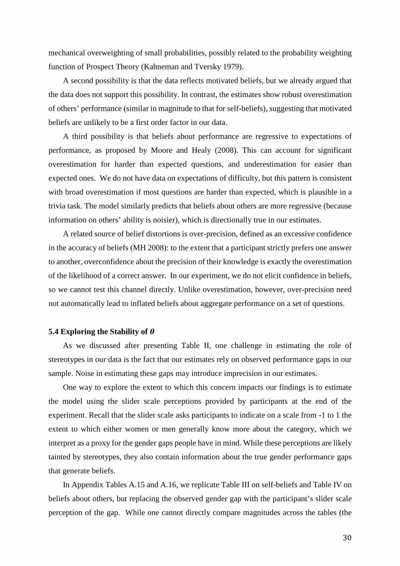
30
mechanical overweighting of small probabilities, possibly related to the probability weighting
function of Prospect Theory (Kahneman and Tversky 1979).
A second possibility is that the data reflects motivated beliefs, but we already argued that
the data does not support this possibility. In contrast, the estimates show robust overestimation
of others’ performance (similar in magnitude to that for self-beliefs), suggesting that motivated
beliefs are unlikely to be a first order factor in our data.
A third possibility is that beliefs about performance are regressive to expectations of
performance, as proposed by Moore and Healy (2008). This can account for significant
overestimation for harder than expected questions, and underestimation for easier than
expected ones. We do not have data on expectations of difficulty, but this pattern is consistent
with broad overestimation if most questions are harder than expected, which is plausible in a
trivia task. The model similarly predicts that beliefs about others are more regressive (because
information on others’ ability is noisier), which is directionally true in our estimates.
A related source of belief distortions is over-precision, defined as an excessive confidence
in the accuracy of beliefs (MH 2008): to the extent that a participant strictly prefers one answer
to another, overconfidence about the precision of their knowledge is exactly the overestimation
of the likelihood of a correct answer. In our experiment, we do not elicit confidence in beliefs,
so we cannot test this channel directly. Unlike overestimation, however, over-precision need
not automatically lead to inflated beliefs about aggregate performance on a set of questions.
5.4 Exploring the Stability of 𝜽𝜽
As we discussed after presenting Table II, one challenge in estimating the role of
stereotypes in our data is the fact that our estimates rely on observed performance gaps in our
sample. Noise in estimating these gaps may introduce imprecision in our estimates.
One way to explore the extent to which this concern impacts our findings is to estimate
the model using the slider scale perceptions provided by participants at the end of the
experiment. Recall that the slider scale asks participants to indicate on a scale from -1 to 1 the
extent to which either women or men generally know more about the category, which we
interpret as a proxy for the gender gaps people have in mind. While these perceptions are likely
tainted by stereotypes, they also contain information about the true gender performance gaps
that generate beliefs.
In Appendix Tables A.15 and A.16, we replicate Table III on self-beliefs and Table IV on
beliefs about others, but replacing the observed gender gap with the participant’s slider scale
perception of the gap. While one cannot directly compare magnitudes across the tables (the
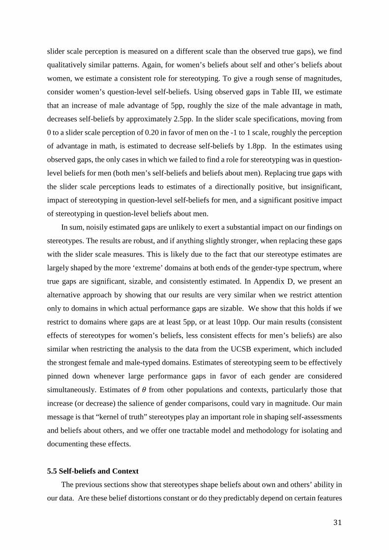
31
slider scale perception is measured on a different scale than the observed true gaps), we find
qualitatively similar patterns. Again, for women’s beliefs about self and other’s beliefs about
women, we estimate a consistent role for stereotyping. To give a rough sense of magnitudes,
consider women’s question-level self-beliefs. Using observed gaps in Table III, we estimate
that an increase of male advantage of 5pp, roughly the size of the male advantage in math,
decreases self-beliefs by approximately 2.5pp. In the slider scale specifications, moving from
0 to a slider scale perception of 0.20 in favor of men on the -1 to 1 scale, roughly the perception
of advantage in math, is estimated to decrease self-beliefs by 1.8pp. In the estimates using
observed gaps, the only cases in which we failed to find a role for stereotyping was in question-
level beliefs for men (both men’s self-beliefs and beliefs about men). Replacing true gaps with
the slider scale perceptions leads to estimates of a directionally positive, but insignificant,
impact of stereotyping in question-level self-beliefs for men, and a significant positive impact
of stereotyping in question-level beliefs about men.
In sum, noisily estimated gaps are unlikely to exert a substantial impact on our findings on
stereotypes. The results are robust, and if anything slightly stronger, when replacing these gaps
with the slider scale measures. This is likely due to the fact that our stereotype estimates are
largely shaped by the more ‘extreme’ domains at both ends of the gender-type spectrum, where
true gaps are significant, sizable, and consistently estimated. In Appendix D, we present an
alternative approach by showing that our results are very similar when we restrict attention
only to domains in which actual performance gaps are sizable. We show that this holds if we
restrict to domains where gaps are at least 5pp, or at least 10pp. Our main results (consistent
effects of stereotypes for women’s beliefs, less consistent effects for men’s beliefs) are also
similar when restricting the analysis to the data from the UCSB experiment, which included
the strongest female and male-typed domains. Estimates of stereotyping seem to be effectively
pinned down whenever large performance gaps in favor of each gender are considered
simultaneously. Estimates of 𝜃𝜃 from other populations and contexts, particularly those that
increase (or decrease) the salience of gender comparisons, could vary in magnitude. Our main
message is that “kernel of truth” stereotypes play an important role in shaping self-assessments
and beliefs about others, and we offer one tractable model and methodology for isolating and
documenting these effects.
5.5 Self-beliefs and Context
The previous sections show that stereotypes shape beliefs about own and others’ ability in
our data. Are these belief distortions constant or do they predictably depend on certain features
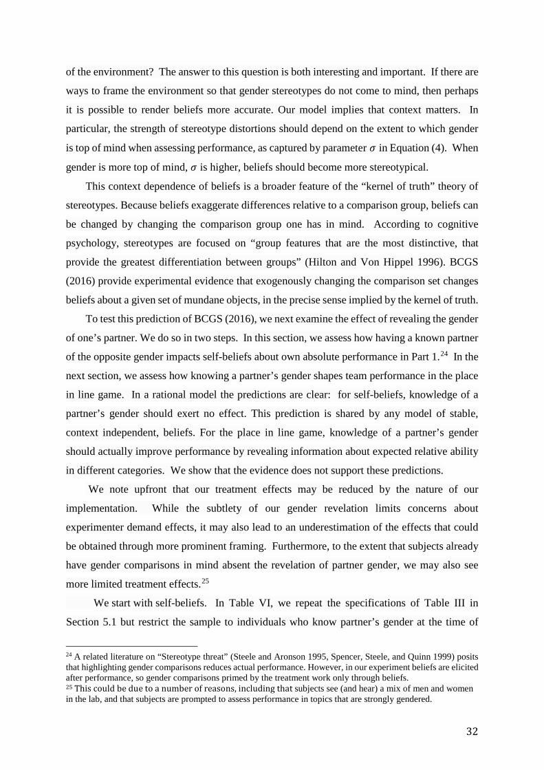
32
of the environment? The answer to this question is both interesting and important. If there are
ways to frame the environment so that gender stereotypes do not come to mind, then perhaps
it is possible to render beliefs more accurate. Our model implies that context matters. In
particular, the strength of stereotype distortions should depend on the extent to which gender
is top of mind when assessing performance, as captured by parameter 𝜎𝜎 in Equation (4). When
gender is more top of mind, 𝜎𝜎 is higher, beliefs should become more stereotypical.
This context dependence of beliefs is a broader feature of the “kernel of truth” theory of
stereotypes. Because beliefs exaggerate differences relative to a comparison group, beliefs can
be changed by changing the comparison group one has in mind. According to cognitive
psychology, stereotypes are focused on “group features that are the most distinctive, that
provide the greatest differentiation between groups” (Hilton and Von Hippel 1996). BCGS
(2016) provide experimental evidence that exogenously changing the comparison set changes
beliefs about a given set of mundane objects, in the precise sense implied by the kernel of truth.
To test this prediction of BCGS (2016), we next examine the effect of revealing the gender
of one’s partner. We do so in two steps. In this section, we assess how having a known partner
of the opposite gender impacts self-beliefs about own absolute performance in Part 1.24 In the
next section, we assess how knowing a partner’s gender shapes team performance in the place
in line game. In a rational model the predictions are clear: for self-beliefs, knowledge of a
partner’s gender should exert no effect. This prediction is shared by any model of stable,
context independent, beliefs. For the place in line game, knowledge of a partner’s gender
should actually improve performance by revealing information about expected relative ability
in different categories. We show that the evidence does not support these predictions.
We note upfront that our treatment effects may be reduced by the nature of our
implementation. While the subtlety of our gender revelation limits concerns about
experimenter demand effects, it may also lead to an underestimation of the effects that could
be obtained through more prominent framing. Furthermore, to the extent that subjects already
have gender comparisons in mind absent the revelation of partner gender, we may also see
more limited treatment effects.25
We start with self-beliefs. In Table VI, we repeat the specifications of Table III in
Section 5.1 but restrict the sample to individuals who know partner’s gender at the time of
24 A related literature on “Stereotype threat” (Steele and Aronson 1995, Spencer, Steele, and Quinn 1999) posits that highlighting gender comparisons reduces actual performance. However, in our experiment beliefs are elicited after performance, so gender comparisons primed by the treatment work only through beliefs. 25 This could be due to a number of reasons, including that subjects see (and hear) a mix of men and women in the lab, and that subjects are prompted to assess performance in topics that are strongly gendered.
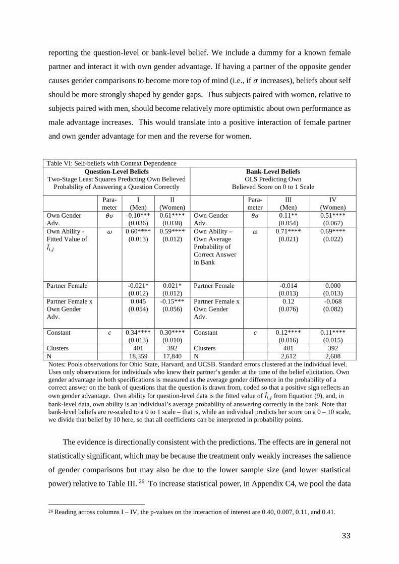
33
reporting the question-level or bank-level belief. We include a dummy for a known female
partner and interact it with own gender advantage. If having a partner of the opposite gender
causes gender comparisons to become more top of mind (i.e., if 𝜎𝜎 increases), beliefs about self
should be more strongly shaped by gender gaps. Thus subjects paired with women, relative to
subjects paired with men, should become relatively more optimistic about own performance as
male advantage increases. This would translate into a positive interaction of female partner
and own gender advantage for men and the reverse for women.
Table VI: Self-beliefs with Context Dependence
Question-Level Beliefs Two-Stage Least Squares Predicting Own Believed
Probability of Answering a Question Correctly
Bank-Level Beliefs OLS Predicting Own
Believed Score on 0 to 1 Scale
Para-meter
I (Men)
II (Women)
Para-meter
III (Men)
IV (Women)
Own Gender Adv.
𝜃𝜃𝜎𝜎 -0.10*** (0.036)
0.61**** (0.038)
Own Gender Adv.
𝜃𝜃𝜎𝜎 0.11** (0.054)
0.51**** (0.067)
Own Ability - Fitted Value of 𝐼𝐼𝑖𝑖,𝑗𝑗
𝜔𝜔 0.60**** (0.013)
0.59**** (0.012)
Own Ability –Own Average Probability of Correct Answer in Bank
𝜔𝜔 0.71**** (0.021)
0.69**** (0.022)
Partner Female -0.021* (0.012)
0.021* (0.012)
Partner Female -0.014 (0.013)
0.000 (0.013)
Partner Female x Own Gender Adv.
0.045 (0.054)
-0.15*** (0.056)
Partner Female x Own Gender Adv.
0.12 (0.076)
-0.068 (0.082)
Constant c 0.34**** (0.013)
0.30**** (0.010)
Constant c 0.12**** (0.016)
0.11**** (0.015)
Clusters 401 392 Clusters 401 392 N 18,359 17,840 N 2,612 2,608 Notes: Pools observations for Ohio State, Harvard, and UCSB. Standard errors clustered at the individual level. Uses only observations for individuals who knew their partner’s gender at the time of the belief elicitation. Own gender advantage in both specifications is measured as the average gender difference in the probability of a correct answer on the bank of questions that the question is drawn from, coded so that a positive sign reflects an own gender advantage. Own ability for question-level data is the fitted value of 𝐼𝐼𝑖𝑖,𝑗𝑗 from Equation (9), and, in bank-level data, own ability is an individual’s average probability of answering correctly in the bank. Note that bank-level beliefs are re-scaled to a 0 to 1 scale – that is, while an individual predicts her score on a 0 – 10 scale, we divide that belief by 10 here, so that all coefficients can be interpreted in probability points.
The evidence is directionally consistent with the predictions. The effects are in general not
statistically significant, which may be because the treatment only weakly increases the salience
of gender comparisons but may also be due to the lower sample size (and lower statistical
power) relative to Table III. 26 To increase statistical power, in Appendix C4, we pool the data
26 Reading across columns I – IV, the p-values on the interaction of interest are 0.40, 0.007, 0.11, and 0.41.
34
for both male and female participants who knew the gender of their partner, regressing self-
beliefs on male advantage in the category, a dummy for female partner, and the interaction of
these two terms. The estimated interaction is of similar magnitude to Table VI, and is now
significant in question-level data and marginally significant in bank-level data.27
To give a sense of magnitudes, we estimate that a woman moving from a gender neutral
category to a moderately male-typed category such as math (male advantage of 0.05) reduces
her believed probability of answering correctly by approximately 2.4pp when paired with a
woman and by 2.9pp when paired with a man. Appendix C4, Table A6 shows that this effect
is not limited to gender: among the sample of participants who received photographs of their
partner, partner ethnicity has an impact on self-beliefs.
The evidence thus points to context dependence in our data. More detailed tests of the
kernel of truth hypothesis and the context dependence of gender stereotypes would involve
finding stronger ways of varying the salience of gender, in particular of reducing gender
comparisons for subjects paired within their own gender. For example, evidence suggests that
women educated at single-sex schools display little if any under-confidence in math (Fryer and
Levitt 2010, Booth and Nolen 2012), perhaps because the gender comparison is less salient
given their experience.
6. Beliefs of Relative Ability and the Consequences for Decision-Making
Our model and our data deal with beliefs of absolute ability: one’s own and partner’s
believed probability of answering correctly. In many decision-making contexts, however, the
beliefs of relative ability may be most predictive. Decisions whether to compete in a
tournament are a function of whether an individual believes she can beat others; decisions
whether to apply for a job or promotion are likely to be a function of believed rank within the
pool of potential candidates. It is then important to check how the patterns in believed absolute
ability we identify translate into beliefs of relative ability. In this section, we first document
how the determinants of beliefs explored in Section 5 – DIM, stereotypes, and context
dependence – combine to produce gender differences in beliefs of relative ability. We then
take this analysis from beliefs to strategic decisions within a group, and examine how our
participants make decisions about when to contribute ideas.
27 In question-level data, the estimated interaction is 0.096 (SE of 0.039, p-value<0.05). In bank level data, the estimated interaction is 0.095 (SE of 0.056, p-value=0.10). See Appendix C4, Table A5 for details.
35
In Figure IV, we present data on beliefs about relative ability, focusing on both partner
gender and category. For each participant who knows the gender of their partner at the time of
belief elicitation, we construct the gap in average beliefs about own ability and average beliefs
about partner’s ability at the category level, weighting the bank-level and question-level data
equally. We ask how this believed ability gap between self and partner varies with partner
gender and category. Panel (a) presents believed relative ability for men with male partners in
blue and with female partners in red. Panel (b) presents the same measures for women. In both
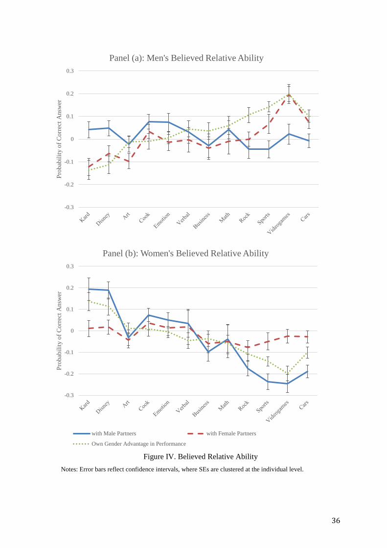
36
Figure IV. Believed Relative Ability Notes: Error bars reflect confidence intervals, where SEs are clustered at the individual level.
-0.3
-0.2
-0.1
0
0.1
0.2
0.3
Prob
abili
ty o
f Cor
rect
Ans
wer
Panel (a): Men's Believed Relative Ability
with Male Partners with Female Partners Male Advantage in Performance
-0.3
-0.2
-0.1
0
0.1
0.2
0.3
Prob
abili
ty o
f Cor
rect
Ans
wer
Panel (b): Women's Believed Relative Ability
with Male Partners with Female Partners
Own Gender Advantage in Performance
37
graphs, we have also added the true gender difference in performance as the dotted green line
for reference. Accurate beliefs for an individual paired with a same gender partner would
average 0 in each category; accurate beliefs for an individual paired with an opposite gender
partner would average the true gender difference in performance – the dotted green line.
Figure IV shows that the patterns of beliefs documented in Section 5 have important
implications for beliefs about relative ability. For men paired with male partners, believed
relative ability is relatively flat across the categories. If anything, men paired with male partners
are relatively more confident in clearly female-typed categories (by an average of 4pp) than in
clearly male-typed categories (by an average of -1pp).28 For men paired with female partners,
the pattern is reversed. Men believe they are less knowledgeable than their female partners in
the clearly female-typed categories (by 9pp on average), and more knowledgeable than their
female partners in male-typed categories (by 9pp on average).29 Relative to the accurate beliefs
benchmark, men are not exaggerating the gender gap in performance – if anything, they
underestimate the extent of their advantage over women in many of the male-typed domains.
When paired with male partners, women believe that they outperform their partner in the
female-typed categories, by 19pp on average, but believe that they are outperformed by their
partner in the male-typed categories – by 20pp. 30 For the extreme categories, there is
exaggeration relative to the true gap (green dotted line). When women are paired with women,
relative beliefs vary less with the category, hovering closer to 0.
These patterns suggest that decisions are likely to be a function of gender stereotypes,
reflected in responsiveness to both the domain, the gender of one’s partner, and the interaction
of the two. We find evidence for this in our data from the place in line game, where measured
beliefs are strongly predictive of willingness to contribute.31 Here, we focus on the implications
of stereotyped beliefs for group performance that follows from place in line decisions.
28 If we regress believed relative ability for men paired with male partners on the gender-type of the category, we can reject that believed relative ability is the same across gender-type with p<0.01. The point estimates and p-value are unchanged if we include all categories (using slider scale to classify male versus female) or only those that are clearly male or female-typed as defined in Section 3. 29 If we regress believed relative ability for men paired with female partners on the gender-type of the category, restricting to clearly male or female-typed, we can reject that believed relative ability is the same across gender-type with p<0.01. If we instead include all categories, the point estimates are 5pp and 8pp, respectively, p<0.01. 30 These estimates are both significantly different from 0, p<0.001, and from each other, p<0.001. Point estimates using all categories are 11p and 19pp, p-value statements unchanged. 31 This is a replication of the findings of Coffman (2014), who finds that beliefs about self and beliefs about partner strongly predict willingness to contribute answers in a very similar paradigm. Appendix Tables A.7 and A.8 in Appendix C explore this relationship in our data, regressing place in line from ability, male advantage in the category, partner gender, and beliefs.
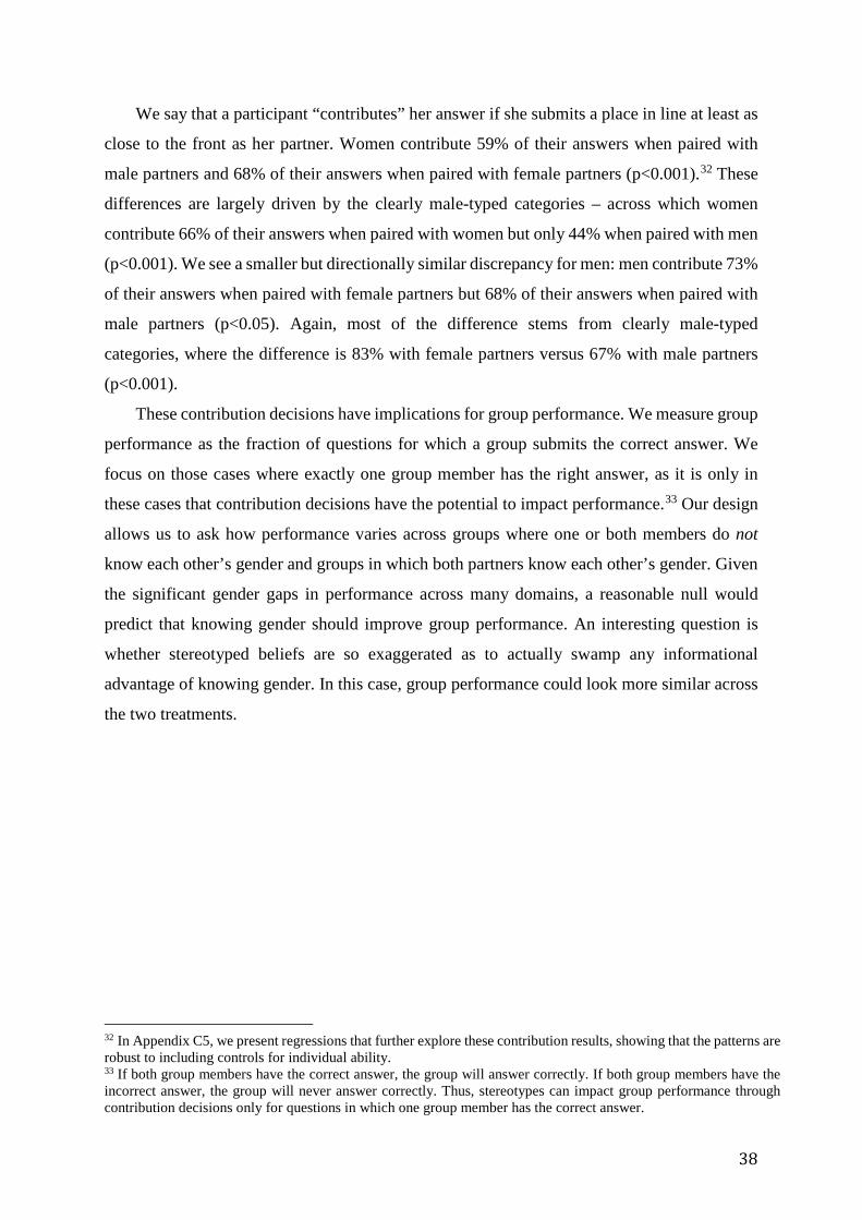
38
We say that a participant “contributes” her answer if she submits a place in line at least as
close to the front as her partner. Women contribute 59% of their answers when paired with
male partners and 68% of their answers when paired with female partners (p<0.001).32 These
differences are largely driven by the clearly male-typed categories – across which women
contribute 66% of their answers when paired with women but only 44% when paired with men
(p<0.001). We see a smaller but directionally similar discrepancy for men: men contribute 73%
of their answers when paired with female partners but 68% of their answers when paired with
male partners (p<0.05). Again, most of the difference stems from clearly male-typed
categories, where the difference is 83% with female partners versus 67% with male partners
(p<0.001).
These contribution decisions have implications for group performance. We measure group
performance as the fraction of questions for which a group submits the correct answer. We
focus on those cases where exactly one group member has the right answer, as it is only in
these cases that contribution decisions have the potential to impact performance.33 Our design
allows us to ask how performance varies across groups where one or both members do not
know each other’s gender and groups in which both partners know each other’s gender. Given
the significant gender gaps in performance across many domains, a reasonable null would
predict that knowing gender should improve group performance. An interesting question is
whether stereotyped beliefs are so exaggerated as to actually swamp any informational
advantage of knowing gender. In this case, group performance could look more similar across
the two treatments.
32 In Appendix C5, we present regressions that further explore these contribution results, showing that the patterns are robust to including controls for individual ability. 33 If both group members have the correct answer, the group will answer correctly. If both group members have the incorrect answer, the group will never answer correctly. Thus, stereotypes can impact group performance through contribution decisions only for questions in which one group member has the correct answer.
39
Figure V. Group Performance
Notes: Error bars reflect confidence intervals, where SEs are clustered at the group level.
Figure V shows the results, both overall and by gender-type of the domain. Overall, both
members knowing each other’s gender has a modest but significant negative impact on group
performance: groups submit the correct answer approximately 2pp less often when they both
know each other’s gender than when they don’t (69% versus 71%, p<0.05). The results for
each sub-group of domains suggest an insignificant, but directionally negative, impact of
knowing gender on group performance. Any advantage of knowing gender is completely
crowded out by the overreaction to information entailed by stereotypes. For instance, just as
Figure IV shows, a woman learning that her partner is male would be too underconfident in
her own relative ability in male-typed categories, translating into fewer contributed answers
and a directionally negative impact on group performance.
7. Conclusion
Despite substantial evidence that, in some domains, men are more overconfident than
women about their ability, the sources of such overconfidence are not completely understood.
Nor do we have a clear understanding of the sources of beliefs about the ability of others, and
why such beliefs are often inaccurate. In this paper, we presented evidence that beliefs about
both oneself and others to a significant extent come from the same two sources. The first
source is stereotyping, and in particular the kernel of truth hypothesis whereby beliefs
exaggerate true aspects of reality. The second source is overestimation of the ability of both
0.5
0.55
0.6
0.65
0.7
0.75
0.8
0.85
Overall Clearly Female-Typed(Kardashian, Disney)
Ambiguous (Verbal,Art, Emotion,
Cooking, Business
Clearly Male-Typed(Math, Rock, Sports,Videogames, Cars)
Shar
e of
Que
stio
ns A
nsw
ered
Cor
rect
ly
Unknown Gender Known Gender
40
oneself and others, which increases with the difficulty of the question, what we called
difficulty-influenced mis-estimation or DIM. Because we collect data not only on beliefs about
oneself but also on beliefs about others, and do so for a variety of difficulties and domains, we
can disentangle these two sources to shed light on beliefs about gender.
Stereotypes cause the participants in our experiments to exaggerate the actual gender
performance gaps, leading women to be much less confident about themselves in domains
where the male advantage is larger. Stereotypes also play a role in explaining men’s
confidence, although not as much as they do for women. Crucially, stereotypes also matter for
beliefs about others. Holding fixed category difficulty, both men and women underestimate the
ability of women relative to men in male-typed domains, and overestimate it in female-typed
domains. We also found that stereotypes are reflected in beliefs about relative and not just
absolute ability, and actually influence behavior. DIM and stereotypes combine to encourage
more self-confident behavior of men, and less self-confident behavior of women, but really
only in male-typed fields.
Disentangling the causes of the gender gap in beliefs may help interpret the existing
evidence, but also inform interventions aimed at narrowing these gaps. To the extent that
stereotypes shape this gap, the reality that actual performance differences between genders are
narrowing, especially at the upper tail, suggests that stereotypes will become less extreme over
time. Role models and other manifestations of similar performance of men and women in the
right tail may have big effects on reducing the gap. Porter and Serra (2017) find a large effect
of female role models on the choice of economics concentration, which is consistent with this
view. In areas where actual differences remain, factors that make gender (or ethnicity, or race)
less top of mind would diminish the effects of stereotypes on beliefs. Although we do not
understand the causes of mis-estimation as well, the Moore Healy model suggests that objective
feedback about ability will diminish the influence of DIM on self-confidence. But if DIM is
driven by factors other than information, such feedback might not help.
Our analysis also suggests that the same factors that shape confidence might also shape
discrimination. Unlike in the standard models of statistical discrimination, our experimental
evidence suggests that beliefs are inaccurate in equilibrium. Recent research on gender
(Behren, Imas, and Rosenberg 2017), ethnicity (Grover, Pallais, and Paviente 2017), and race
(Arnold, Dobbie, and Yang 2017) shows that inaccurate beliefs that look very much like
stereotypes are at the heart of discriminatory practices. Because our evidence shows that
beliefs about oneself and others are shaped by very similar psychological forces, the
mechanisms that reduce the gap in self-confidence are also likely to reduce discrimination.
41
Perhaps the central message of our analysis, then, is the importance of psychological
distortions in beliefs about gender. Research on self-confidence has appreciated the central
role of such distortions for a long time. Stereotypes might be a useful concept for organizing
and developing this analysis, in part because they point to the close relationship between beliefs
and reality that varies across domains. Research on discrimination and the centrality of
inaccurate beliefs about others has been more recent, and here as well stereotypes offer a new
conceptualization. Our principal conclusion is that stereotyping and distortions related to task
difficulty provide a unified framework for the study of distorted beliefs. By showing the role
of these two factors, our analysis suggests a strategy for unification of disparate findings, but
also of moving forward with both empirical research and policy.
Disclosure: We have reported all treatments conducted, all measures and materials are available in Appendix A, and data exclusions are described in Table I. At OSU, we ran 20 sessions, targeting approximately 400 total participants. At Harvard we ran until we had collected data from 250 participants. At UCSB, we ran until we had collected data from at least 200 women and 200 men who had attended high school in the United States.
42
References
Acker, Daniella & Nigel W. Duck. (2008). Cross-cultural overconfidence and biased self-
attribution. The Journal of Socio-Economics, 37, 1815 – 1824.
Arnold, David, Will Dobbie, & Crystal S. Yang. (2017). Racial bias in bail decisions.
Working paper.
Arrow, Kenneth. (1998). What has economics to say about racial discrimination? Journal of
Economic Perspectives, 12(2), 91 – 100.
Barber, Brad M. & Terrance Odean. (2001). Boys will be boys: Gender, overconfidence, and
common stock investment. Quarterly Journal of Economics, 116(1), 261-292.
Benoit, Jean-Pierre & Juan Dubra. (2011). Apparent overconfidence. Econometrica, 79(5),
1591 – 1625.
Beyer, Sylvia. (1990). Gender differences in the accuracy of self-evaluations of
performance. Journal of Personality and Social Psychology, 59(5), 960-970.
Beyer, Sylvia. (1998). Gender differences in self-perception and negative recall biases. Sex
Roles, 38(1-2), 103-133.
Beyer, Sylvia, & Edward M. Bowden. (1997). Gender differences in self-perceptions:
Convergent evidence from three measures of accuracy and bias. Personality and Social
Psychology Bulletin, 23(2), 157-172
Bohnet, Iris, & Bruno S. Frey. (1999). Social distance and other-regarding behavior in
dictator games: Comment. American Economic Review, 89(1), 335-339.
Bohren, J. Aislinn, Alex Imas, and Michael Rosenberg. (2017). The Dynamics of
Discrimination: Theory and Evidence. Working paper.
Bordalo, Pedro, Katherine B. Coffman, Nicola Gennaioli, & Andrei Shleifer. (2016).
Stereotypes. The Quarterly Journal of Economics, 131(4), 1753-1794.
Booth, Allison, and Patrick Nolen. (2012). Choosing to compete: how different are girls and
boys?. Journal of Economic Behavior and Organization, 81 (2): 542 – 555.
Buser, Thomas, Muriel Niederle, & Hessel Oosterbeek. (2014). Gender, competitiveness, and
career choices. The Quarterly Journal of Economics, 129(3), 1409 – 1447.
Campbell, Nancy K. & Gail Hackett. (1986). The effects of mathematics task performance on
math self-efficacy and task interest. Journal of Vocational Behavior, 28(2), 149 – 162.
Carrell, Scott E., Marianne E. Page, & James E. West. (2010). Sex and science: how
professor gender perpetuates the gender gap. The Quarterly Journal of Economics, 3(1),
1101-1144.
43
Coffman, Katherine B. (2014). Evidence on self-stereotyping and the contribution of
ideas. The Quarterly Journal of Economics, 129(4), 1625-1660.
The College Board. (2013). 2013 College-Bound Seniors: Total Group Profile Report.
Retrieved from
http://media.collegeboard.com/digitalServices/pdf/research/2013/TotalGroup-2013.pdf
Deaux, Kay & Elizabeth Farris. (1977). Attributing causes for one's own performance: The
effects of sex, norms, and outcome. Journal of Research in Personality, 11(1), 59-72.
Dreber, Anna, Emma von Essen, & Eva Ranehill. (2011). Outrunning the gender gap—boys
and girls compete equally. Experimental Economics, 14(4), 567-582.
Eccles, Jacquelynne S., Janis E. Jacobs, & Rena D. Harold. (1990). Gender roles stereotypes,
expectancy effects, and parents’ socialization of gender differences. Journal of Social
Issues, 46(2), 183-201.
Fennema, Elizabeth H. & Julia A. Sherman. (1978). Sex-related differences in mathematics
achievement and related factors: a further study. Journal for Research in Mathematics
Education, 9(3), 189-203.
Fryer, Roland, and Steve Levitt. (2010). An empirical analysis of the gender gap in
mathematics. American Economic Journal: applied economics, 2(2), 210 – 240.
Glover, Dylan, Amanda Pallais, & William Pariente. (2017). Discrimination as a self-
fulfilling prophecy: evidence from French grocery stores. Quarterly Journal of
Economics, 132 (3): 1219 – 1260.
Goldin, Claudia, Lawrence F. Katz, & Ilyana Kuziemko. (2006). The homecoming of
American college women: the reversal of the college gender gap. Journal of Economic
Perspectives, 20(4), 133-156.
Grosse, Niels D., & Gerhard Riener. (2010). Explaining gender differences in
competitiveness: Gender-task stereotypes. Jena Economic Research Papers 2010 – 017.
Guiso, Luigi, Ferdinando Monte, Paola Sapienza, & Luigi Zingales. (2008). Culture, gender,
and math. Science, 320(5880), 1164-1165.
Hall, Judith A., & David Matsumoto. (2004). Gender differences in judgments of multiple
emotions from facial expressions. Emotion, 4(2), 201-206.
Lundeberg, Mary A., Paul W. Fox, & Judith Punćcohaŕ. (1994). Highly confident but wrong:
gender differences and similarities in confidence judgments. Journal of Educational
Psychology, 86(1), 114-121.
Kahneman, Daniel, & Amos Tversky. (1972). Subjective probability: A Judgment of
Representativeness. Cognitive Psychology, 3(3), 430 – 454.
44
Kahneman, Daniel, & Amos Tversky. (1979). Prospect theory: An analysis of decision under
risk. Econometrica, 47(2), 263-292.
Keltner, Dacher & Robert J. Robinson. (1996). Extremism, Power, and the Imagined Basis of
Social Conflict. Current Directions in Psychological Science, 5(4), 101 – 105.
Kiefer, Amy K. & Denise Sekaquaptewa. (2007). Implicit stereotypes, gender identification,
and math-related outcomes a prospective study of female college students. Psychological
Science, 18(1), 13-18.
Mobius Markus M., Muriel Niederle, Paul Niehaus, & Tanya S. Rosenblat. (2014).
Managing self-confidence. Working Paper.
Moore, Don A., & Paul J. Healy. (2008). The trouble with overconfidence. Psychological
Review, 115(2), 502-517.
Niederle, Muriel, & Lise Vesterlund. (2007). Do women shy away from competition? Do
men compete too much?, The Quarterly Journal of Economics, 122(3), 1067-1101.
Nosek, Brian A., Frederick L. Smyth, N. Sriram, Nicole M. Lindner, Thierry Devos, Alfonso
Ayala, Yoav Bar-Anan et al. (2009). National differences in gender–science stereotypes
predict national sex differences in science and math achievement. Proceedings of the
National Academy of Sciences, 106(26), 10593-10597.
Phelps, Edmund S. (1972). The statistical theory of racism and sexism. The American
Economic Review, 62(4), 659 – 661.
Porter, Catherine & Danila Serra. (2018). Gender differences in the choice of major: the
importance of female role models. Working paper.
Pulford, Briony D., & Andrew M. Colman. (1997). Overconfidence: Feedback and item
difficulty effects. Personality and Individual Differences, 23(1), 125-133.
Reuben, Ernesto, Paola Sapienza, & Luigi Zingales. (2014). How stereotypes impair
women’s careers in science. Proceedings of the National Academy of Sciences, 111(12),
4403-4408.
Shurchkov, Olga. (2012). Under pressure: gender differences in output quality and quantity
under competition and time constraints. Journal of the European Economic
Association, 10(5), 1189-1213.
Spencer, Steven J., Claude M. Steele, & Diane M. Quinn. (1999). Stereotype threat and
women's math performance. Journal of Experimental Social Psychology, 35(1), 4-28.
Steele, Claude M., & Joshua Aronson. (1995). Stereotype threat and the intellectual test
performance of African Americans. Journal of Personality and Social Psychology,
69(5), 797-811.
45
FOR ONLINE PUBLICATION
Appendix A: Experimental Instructions and Materials (available in separate file)
Appendix B: Online Experiment on Social Desirability Bias
The beliefs reported in the experiment may be partially shaped by social norms, which
may discourage a participant from truthfully reporting believed gender differences in
performance. While we use incentives and anonymity to reduce such concerns, we cannot rule
them out. To examine this issue, we ran an experiment online. We had two main goals. First,
we were interested in understanding whether the patterns of beliefs that we observed in our
samples of college students resembled beliefs patterns from a broader population. Second, we
wanted to collect data on the role that social desirability bias might play in determining stated
beliefs.
The experiment is a simplified version of Part 1 of the laboratory experiments we ran. It
was conducted on Amazon Mechanical Turk. We use the same questions from the six
categories in the OSU and Harvard experiment: Art, Verbal Skills, Emotion Recognition,
Mathematics, Business, and Sports. To reduce the length of the study, each participant answers
a subset of five of the ten questions in each of the six categories. They are paid $0.25 for every
correct answer they submit.
After, they are asked about their own and others’ performance. Specifically, they are asked
to guess their own score (out of 5) in each category. They are then asked to guess the score in
each category for a randomly-drawn female MTurk worker and a randomly-drawn male MTurk
worker. The order of these two beliefs questions about others is randomized at the individual
level. These beliefs questions are unincentivized.
Finally, we attempt to understand whether there may be social desirability bias associated
with stating beliefs about gender differences in ability. We adapt the measure proposed by
Krupka and Weber (2013) to elicit norms. Participants are asked: “Suppose someone thought
that [insert gender] knew more about [insert category] than [insert opposite gender]. How
reluctant do you think they would be to announce this to others?”. Participants use a sliding
scale with 7 places, with 1 labeled “Not at all Reluctant” and 7 labeled “Extremely Reluctant”
to indicate their answer. Each participant sees six of these questions, one for each category. We
randomize at the participant level whether they see versions of each question that ask about
female advantages (women knew more) or male advantages (men knew more). The key is that
we care about how participants perceive the social acceptability of reporting beliefs of gender
differences. We are not interested in whether participants believe these statements are likely to
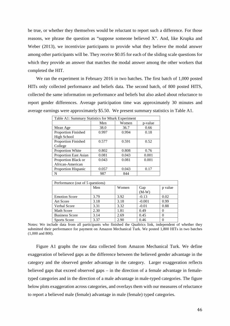
46
be true, or whether they themselves would be reluctant to report such a difference. For those
reasons, we phrase the question as “suppose someone believed X”. And, like Krupka and
Weber (2013), we incentivize participants to provide what they believe the modal answer
among other participants will be. They receive $0.05 for each of the sliding scale questions for
which they provide an answer that matches the modal answer among the other workers that
completed the HIT.
We ran the experiment in February 2016 in two batches. The first batch of 1,000 posted
HITs only collected performance and beliefs data. The second batch, of 800 posted HITS,
collected the same information on performance and beliefs but also asked about reluctance to
report gender differences. Average participation time was approximately 30 minutes and
average earnings were approximately $5.50. We present summary statistics in Table A1. Table A1: Summary Statistics for Mturk Experiment Men Women p-value Mean Age 38.0 36.7 0.66 Proportion Finished High School
0.997 0.994 0.18
Proportion Finished College
0.577 0.591 0.52
Proportion White 0.802 0.808 0.76 Proportion East Asian 0.081 0.043 0.001 Proportion Black or African-American
0.043 0.081 0.001
Proportion Hispanic 0.057 0.043 0.17 N 987 844 Performance (out of 5 questions) Men Women Gap
(M-W) p value
Emotion Score 3.79 3.92 -0.13 0.02 Art Score 3.18 3.18 -0.001 0.99 Verbal Score 3.31 3.32 -0.01 0.88 Math Score 2.30 1.81 0.49 0 Business Score 3.14 2.69 0.45 0 Sports Score 3.37 2.90 0.46 0
Notes: We include data from all participants who finished the Qualtrics link, independent of whether they submitted their performance for payment on Amazon Mechanical Turk. We posted 1,800 HITs in two batches (1,000 and 800).
Figure A1 graphs the raw data collected from Amazon Mechanical Turk. We define
exaggeration of believed gaps as the difference between the believed gender advantage in the
category and the observed gender advantage in the category. Larger exaggeration reflects
believed gaps that exceed observed gaps – in the direction of a female advantage in female-
typed categories and in the direction of a male advantage in male-typed categories. The figure
below plots exaggeration across categories, and overlays them with our measures of reluctance
to report a believed male (female) advantage in male (female) typed categories.
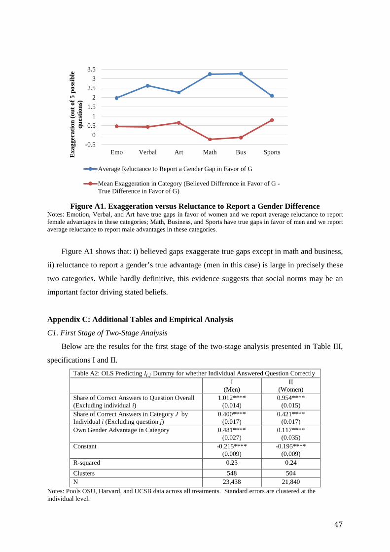
47
Figure A1. Exaggeration versus Reluctance to Report a Gender Difference
Notes: Emotion, Verbal, and Art have true gaps in favor of women and we report average reluctance to report female advantages in these categories; Math, Business, and Sports have true gaps in favor of men and we report average reluctance to report male advantages in these categories.
Figure A1 shows that: i) believed gaps exaggerate true gaps except in math and business,
ii) reluctance to report a gender’s true advantage (men in this case) is large in precisely these
two categories. While hardly definitive, this evidence suggests that social norms may be an
important factor driving stated beliefs.
Appendix C: Additional Tables and Empirical Analysis
C1. First Stage of Two-Stage Analysis
Below are the results for the first stage of the two-stage analysis presented in Table III,
specifications I and II. Table A2: OLS Predicting 𝐼𝐼𝑖𝑖,𝑗𝑗 Dummy for whether Individual Answered Question Correctly I
(Men) II
(Women) Share of Correct Answers to Question Overall (Excluding individual i)
1.012**** (0.014)
0.954**** (0.015)
Share of Correct Answers in Category J by Individual i (Excluding question j)
0.400**** (0.017)
0.421**** (0.017)
Own Gender Advantage in Category 0.481**** (0.027)
0.117**** (0.035)
Constant -0.215**** (0.009)
-0.195**** (0.009)
R-squared 0.23 0.24 Clusters 548 504 N 23,438 21,840
Notes: Pools OSU, Harvard, and UCSB data across all treatments. Standard errors are clustered at the individual level.
-0.50
0.51
1.52
2.53
3.5
Emo Verbal Art Math Bus SportsExa
gger
atio
n (o
ut o
f 5 p
ossi
ble
ques
tions
)
Average Reluctance to Report a Gender Gap in Favor of G
Mean Exaggeration in Category (Believed Difference in Favor of G -True Difference in Favor of G)
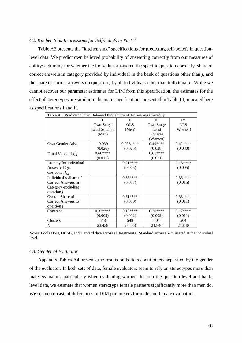
48
C2. Kitchen Sink Regressions for Self-beliefs in Part 3
Table A3 presents the “kitchen sink” specifications for predicting self-beliefs in question-
level data. We predict own believed probability of answering correctly from our measures of
ability: a dummy for whether the individual answered the specific question correctly, share of
correct answers in category provided by individual in the bank of questions other than j, and
the share of correct answers on question j by all individuals other than individual i. While we
cannot recover our parameter estimates for DIM from this specification, the estimates for the
effect of stereotypes are similar to the main specifications presented in Table III, repeated here
as specifications I and II. Notes: Pools OSU, UCSB, and Harvard data across all treatments. Standard errors are clustered at the individual level.
C3. Gender of Evaluator
Appendix Tables A4 presents the results on beliefs about others separated by the gender
of the evaluator. In both sets of data, female evaluators seem to rely on stereotypes more than
male evaluators, particularly when evaluating women. In both the question-level and bank-
level data, we estimate that women stereotype female partners significantly more than men do.
We see no consistent differences in DIM parameters for male and female evaluators.
Table A3: Predicting Own Believed Probability of Answering Correctly I
Two-Stage Least Squares
(Men)
II OLS
(Men)
III Two-Stage
Least Squares
(Women)
IV OLS
(Women)
Own Gender Adv. -0.039 (0.026)
0.093**** (0.025)
0.49**** (0.028)
0.42**** (0.030)
Fitted Value of 𝐼𝐼𝑖𝑖,𝑗𝑗 0.60**** (0.011)
0.61**** (0.011)
Dummy for Individual Answered Qn. Correctly, 𝐼𝐼𝑖𝑖 ,𝑗𝑗
0.21**** (0.005)
0.18**** (0.005)
Individual’s Share of Correct Answers in Category excluding question j
0.36**** (0.017)
0.35**** (0.015)
Overall Share of Correct Answers to question j
0.31**** (0.010)
0.33**** (0.011)
Constant 0.33**** (0.009)
0.19**** (0.012)
0.30**** (0.009)
0.17**** (0.011)
Clusters 548 548 504 504 N 23,438 23,438 21,840 21,840
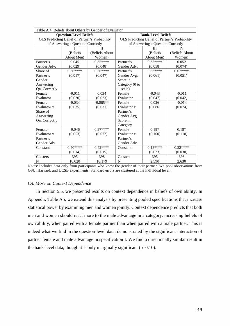
49
Table A.4: Beliefs about Others by Gender of Evaluator Question-Level Beliefs
OLS Predicting Belief of Partner’s Probability of Answering a Question Correctly
Bank-Level Beliefs OLS Predicting Belief of Partner’s Probability
of Answering a Question Correctly I
(Beliefs About Men)
II (Beliefs About
Women)
III (Beliefs
About Men)
IV (Beliefs About
Women) Partner’s Gender Adv.
0.045 (0.029)
0.35**** (0.048)
Partner’s Gender Adv.
0.35**** (0.058)
0.052 (0.074)
Share of Partner’s Gender Answering Qn. Correctly
0.36**** (0.017)
0.36**** (0.047)
Partner’s Gender Avg. Score in Category (0 to 1 scale)
0.63**** (0.061)
0.62**** (0.051)
Female Evaluator
-0.011 (0.020)
0.034 (0.023)
Female Evaluator
-0.043 (0.047)
-0.011 (0.042)
Female Evaluator x Share of Answering Qn. Correctly
-0.034 (0.025)
-0.065** (0.031)
Female Evaluator x Partner’s Gender Avg. Score in Category
0.026 (0.086)
-0.014 (0.074)
Female Evaluator x Partner’s Gender Adv.
-0.046 (0.053)
0.27**** (0.072)
Female Evaluator x Partner’s Gender Adv.
0.19* (0.100)
0.18* (0.110)
Constant 0.40**** (0.014)
0.42**** (0.015)
Constant 0.18**** (0.033)
0.22**** (0.030)
Clusters 395 398 Clusters 395 398 N 18,020 18,179 N 2,590 2,630
Notes: Includes data only from participants who knew the gender of their partner. We pool observations from OSU, Harvard, and UCSB experiments. Standard errors are clustered at the individual level.
C4. More on Context Dependence
In Section 5.5, we presented results on context dependence in beliefs of own ability. In
Appendix Table A5, we extend this analysis by presenting pooled specifications that increase
statistical power by examining men and women jointly. Context dependence predicts that both
men and women should react more to the male advantage in a category, increasing beliefs of
own ability, when paired with a female partner than when paired with a male partner. This is
indeed what we find in the question-level data, demonstrated by the significant interaction of
partner female and male advantage in specification I. We find a directionally similar result in
the bank-level data, though it is only marginally significant (p=0.10).
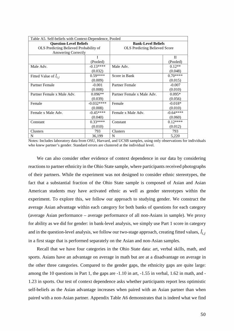
50
Table A5. Self-beliefs with Context-Dependence, Pooled
Question-Level Beliefs OLS Predicting Believed Probability of
Answering Correctly
Bank-Level Beliefs OLS Predicting Believed Score
I (Pooled)
II (Pooled)
Male Adv. -0.13**** (0.032)
Male Adv. 0.12** (0.048)
Fitted Value of 𝐼𝐼𝑖𝑖,𝑗𝑗 0.59**** (0.009)
Score in Bank 0.70**** (0.015)
Partner Female -0.001 (0.008)
Partner Female -0.007 (0.010)
Partner Female x Male Adv. 0.096** (0.039)
Partner Female x Male Adv. 0.095* (0.056)
Female -0.032**** (0.008)
Female -0.018* (0.010)
Female x Male Adv. -0.45**** (0.040)
Female x Male Adv. -0.64**** (0.060)
Constant 0.33**** (0.010)
Constant 0.12**** (0.012)
Clusters 793 Clusters 793 N 36,199 N 5,220
Notes: Includes laboratory data from OSU, Harvard, and UCSB samples, using only observations for individuals who knew partner’s gender. Standard errors are clustered at the individual level.
We can also consider other evidence of context dependence in our data by considering
reactions to partner ethnicity in the Ohio State sample, where participants received photographs
of their partners. While the experiment was not designed to consider ethnic stereotypes, the
fact that a substantial fraction of the Ohio State sample is composed of Asian and Asian
American students may have activated ethnic as well as gender stereotypes within the
experiment. To explore this, we follow our approach to studying gender. We construct the
average Asian advantage within each category for both banks of questions for each category
(average Asian performance – average performance of all non-Asians in sample). We proxy
for ability as we did for gender: in bank-level analysis, we simply use Part 1 score in category
and in the question-level analysis, we follow our two-stage approach, creating fitted values, 𝐼𝐼𝑖𝑖,𝑗𝑗
in a first stage that is performed separately on the Asian and non-Asian samples.
Recall that we have four categories in the Ohio State data: art, verbal skills, math, and
sports. Asians have an advantage on average in math but are at a disadvantage on average in
the other three categories. Compared to the gender gaps, the ethnicity gaps are quite large:
among the 10 questions in Part 1, the gaps are -1.10 in art, -1.55 in verbal, 1.62 in math, and -
1.23 in sports. Our test of context dependence asks whether participants report less optimistic
self-beliefs as the Asian advantage increases when paired with an Asian partner than when
paired with a non-Asian partner. Appendix Table A6 demonstrates that is indeed what we find
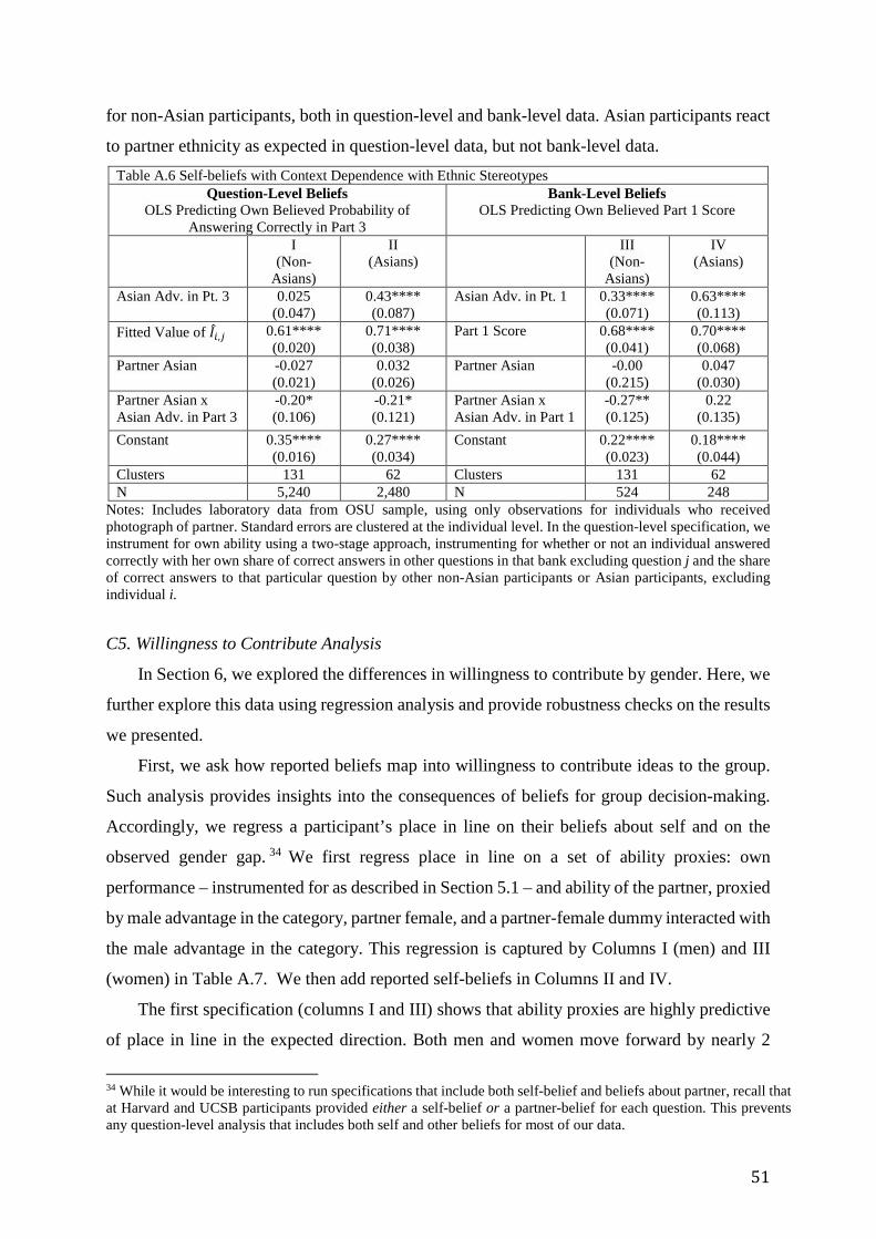
51
for non-Asian participants, both in question-level and bank-level data. Asian participants react
to partner ethnicity as expected in question-level data, but not bank-level data. Table A.6 Self-beliefs with Context Dependence with Ethnic Stereotypes
Question-Level Beliefs OLS Predicting Own Believed Probability of
Answering Correctly in Part 3
Bank-Level Beliefs OLS Predicting Own Believed Part 1 Score
I (Non-
Asians)
II (Asians)
III (Non-
Asians)
IV (Asians)
Asian Adv. in Pt. 3 0.025 (0.047)
0.43**** (0.087)
Asian Adv. in Pt. 1 0.33**** (0.071)
0.63**** (0.113)
Fitted Value of 𝐼𝐼𝑖𝑖,𝑗𝑗 0.61**** (0.020)
0.71**** (0.038)
Part 1 Score 0.68**** (0.041)
0.70**** (0.068)
Partner Asian -0.027 (0.021)
0.032 (0.026)
Partner Asian -0.00 (0.215)
0.047 (0.030)
Partner Asian x Asian Adv. in Part 3
-0.20* (0.106)
-0.21* (0.121)
Partner Asian x Asian Adv. in Part 1
-0.27** (0.125)
0.22 (0.135)
Constant 0.35**** (0.016)
0.27**** (0.034)
Constant 0.22**** (0.023)
0.18**** (0.044)
Clusters 131 62 Clusters 131 62 N 5,240 2,480 N 524 248
Notes: Includes laboratory data from OSU sample, using only observations for individuals who received photograph of partner. Standard errors are clustered at the individual level. In the question-level specification, we instrument for own ability using a two-stage approach, instrumenting for whether or not an individual answered correctly with her own share of correct answers in other questions in that bank excluding question j and the share of correct answers to that particular question by other non-Asian participants or Asian participants, excluding individual i.
C5. Willingness to Contribute Analysis
In Section 6, we explored the differences in willingness to contribute by gender. Here, we
further explore this data using regression analysis and provide robustness checks on the results
we presented.
First, we ask how reported beliefs map into willingness to contribute ideas to the group.
Such analysis provides insights into the consequences of beliefs for group decision-making.
Accordingly, we regress a participant’s place in line on their beliefs about self and on the
observed gender gap. 34 We first regress place in line on a set of ability proxies: own
performance – instrumented for as described in Section 5.1 – and ability of the partner, proxied
by male advantage in the category, partner female, and a partner-female dummy interacted with
the male advantage in the category. This regression is captured by Columns I (men) and III
(women) in Table A.7. We then add reported self-beliefs in Columns II and IV.
The first specification (columns I and III) shows that ability proxies are highly predictive
of place in line in the expected direction. Both men and women move forward by nearly 2
34 While it would be interesting to run specifications that include both self-belief and beliefs about partner, recall that at Harvard and UCSB participants provided either a self-belief or a partner-belief for each question. This prevents any question-level analysis that includes both self and other beliefs for most of our data.
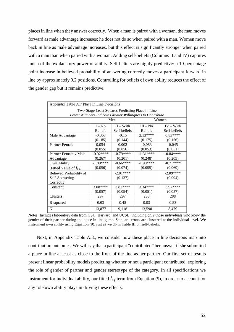
52
places in line when they answer correctly. When a man is paired with a woman, the man moves
forward as male advantage increases; he does not do so when paired with a man. Women move
back in line as male advantage increases, but this effect is significantly stronger when paired
with a man than when paired with a woman. Adding self-beliefs (Columns II and IV) captures
much of the explanatory power of ability. Self-beliefs are highly predictive: a 10 percentage
point increase in believed probability of answering correctly moves a participant forward in
line by approximately 0.2 positions. Controlling for beliefs of own ability reduces the effect of
the gender gap but it remains predictive.
Appendix Table A.7 Place in Line Decisions
Two-Stage Least Squares Predicting Place in Line Lower Numbers Indicate Greater Willingness to Contribute
Men Women I – No
Beliefs II – With
Self-beliefs III – No Beliefs
IV – With Self-beliefs
Male Advantage -0.063 (0.185)
-0.15 (0.144)
2.13**** (0.175)
0.83**** (0.156)
Partner Female 0.054 (0.055)
0.002 (0.056)
-0.083 (0.053)
-0.045 (0.051)
Partner Female x Male Advantage
-0.92**** (0.267)
-0.79**** (0.201)
-1.31**** (0.248)
-0.84**** (0.205)
Own Ability (Fitted Value of 𝐼𝐼𝑖𝑖,𝑗𝑗)
-1.80**** (0.056)
-0.66**** (0.074)
-1.90**** (0.055)
-0.71**** (0.069)
Believed Probability of Self Answering Correctly
-2.01**** (0.137)
-2.09**** (0.094)
Constant 3.08**** (0.057)
3.82**** (0.094)
3.34**** (0.051)
3.97**** (0.057)
Clusters 297 297 288 288 R-squared 0.03 0.48 0.03 0.53 N 13,877 9,118 13,598 8,479
Notes: Includes laboratory data from OSU, Harvard, and UCSB, including only those individuals who knew the gender of their partner during the place in line game. Standard errors are clustered at the individual level. We instrument own ability using Equation (9), just as we do in Table III on self-beliefs.
Next, in Appendix Table A.8., we consider how these place in line decisions map into
contribution outcomes. We will say that a participant “contributed” her answer if she submitted
a place in line at least as close to the front of the line as her partner. Our first set of results
present linear probability models predicting whether or not a participant contributed, exploring
the role of gender of partner and gender stereotype of the category. In all specifications we
instrument for individual ability, our fitted 𝐼𝐼𝑖𝑖,𝑗𝑗 term from Equation (9), in order to account for
any role own ability plays in driving these effects.
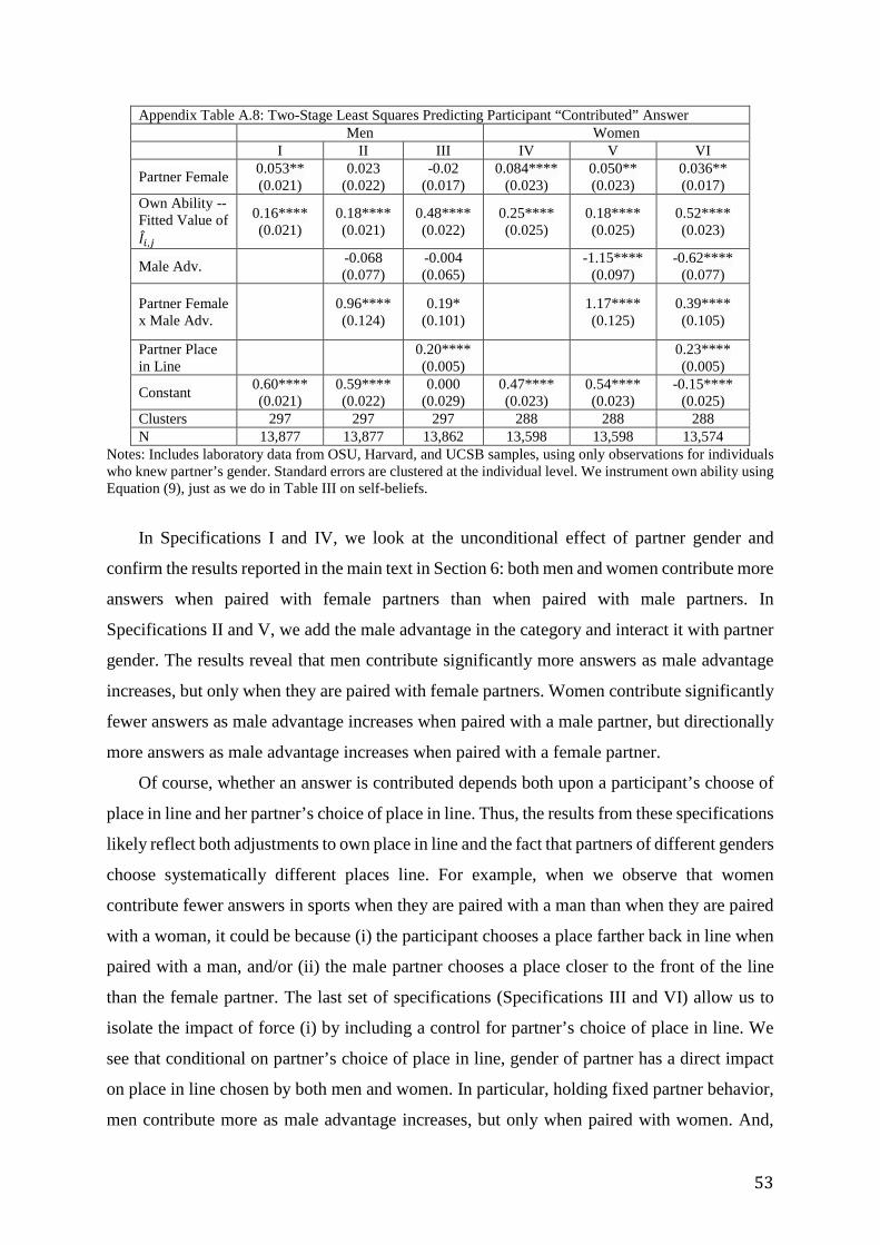
53
Appendix Table A.8: Two-Stage Least Squares Predicting Participant “Contributed” Answer Men Women I II III IV V VI
Partner Female 0.053** (0.021)
0.023 (0.022)
-0.02 (0.017)
0.084**** (0.023)
0.050** (0.023)
0.036** (0.017)
Own Ability -- Fitted Value of 𝐼𝐼𝑖𝑖,𝑗𝑗
0.16**** (0.021)
0.18**** (0.021)
0.48**** (0.022)
0.25**** (0.025)
0.18**** (0.025)
0.52**** (0.023)
Male Adv. -0.068 (0.077)
-0.004 (0.065) -1.15****
(0.097) -0.62****
(0.077)
Partner Female x Male Adv.
0.96**** (0.124)
0.19* (0.101) 1.17****
(0.125) 0.39**** (0.105)
Partner Place in Line 0.20****
(0.005) 0.23**** (0.005)
Constant 0.60**** (0.021)
0.59**** (0.022)
0.000 (0.029)
0.47**** (0.023)
0.54**** (0.023)
-0.15**** (0.025)
Clusters 297 297 297 288 288 288 N 13,877 13,877 13,862 13,598 13,598 13,574
Notes: Includes laboratory data from OSU, Harvard, and UCSB samples, using only observations for individuals who knew partner’s gender. Standard errors are clustered at the individual level. We instrument own ability using Equation (9), just as we do in Table III on self-beliefs.
In Specifications I and IV, we look at the unconditional effect of partner gender and
confirm the results reported in the main text in Section 6: both men and women contribute more
answers when paired with female partners than when paired with male partners. In
Specifications II and V, we add the male advantage in the category and interact it with partner
gender. The results reveal that men contribute significantly more answers as male advantage
increases, but only when they are paired with female partners. Women contribute significantly
fewer answers as male advantage increases when paired with a male partner, but directionally
more answers as male advantage increases when paired with a female partner.
Of course, whether an answer is contributed depends both upon a participant’s choose of
place in line and her partner’s choice of place in line. Thus, the results from these specifications
likely reflect both adjustments to own place in line and the fact that partners of different genders
choose systematically different places line. For example, when we observe that women
contribute fewer answers in sports when they are paired with a man than when they are paired
with a woman, it could be because (i) the participant chooses a place farther back in line when
paired with a man, and/or (ii) the male partner chooses a place closer to the front of the line
than the female partner. The last set of specifications (Specifications III and VI) allow us to
isolate the impact of force (i) by including a control for partner’s choice of place in line. We
see that conditional on partner’s choice of place in line, gender of partner has a direct impact
on place in line chosen by both men and women. In particular, holding fixed partner behavior,
men contribute more as male advantage increases, but only when paired with women. And,
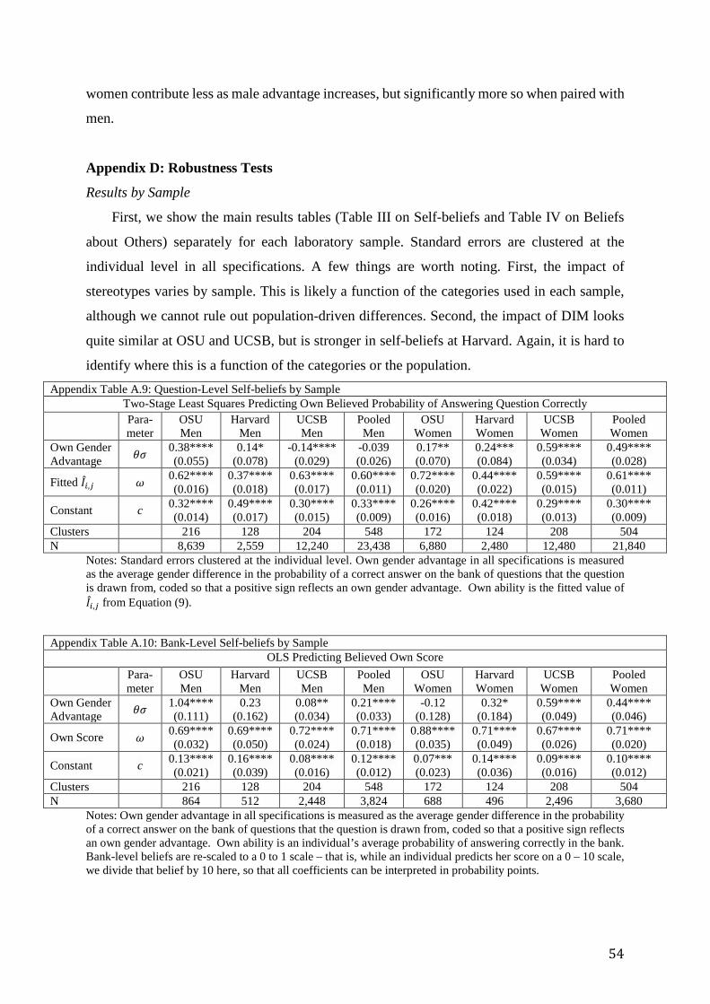
54
women contribute less as male advantage increases, but significantly more so when paired with
men.
Appendix D: Robustness Tests
Results by Sample
First, we show the main results tables (Table III on Self-beliefs and Table IV on Beliefs
about Others) separately for each laboratory sample. Standard errors are clustered at the
individual level in all specifications. A few things are worth noting. First, the impact of
stereotypes varies by sample. This is likely a function of the categories used in each sample,
although we cannot rule out population-driven differences. Second, the impact of DIM looks
quite similar at OSU and UCSB, but is stronger in self-beliefs at Harvard. Again, it is hard to
identify where this is a function of the categories or the population. Appendix Table A.9: Question-Level Self-beliefs by Sample
Two-Stage Least Squares Predicting Own Believed Probability of Answering Question Correctly
Para-meter
OSU Men
Harvard Men
UCSB Men
Pooled Men
OSU Women
Harvard Women
UCSB Women
Pooled Women
Own Gender Advantage 𝜃𝜃𝜎𝜎 0.38****
(0.055) 0.14*
(0.078) -0.14****
(0.029) -0.039 (0.026)
0.17** (0.070)
0.24*** (0.084)
0.59**** (0.034)
0.49**** (0.028)
Fitted 𝐼𝐼𝑖𝑖,𝑗𝑗 𝜔𝜔 0.62**** (0.016)
0.37**** (0.018)
0.63**** (0.017)
0.60**** (0.011)
0.72**** (0.020)
0.44**** (0.022)
0.59**** (0.015)
0.61**** (0.011)
Constant c 0.32**** (0.014)
0.49**** (0.017)
0.30**** (0.015)
0.33**** (0.009)
0.26**** (0.016)
0.42**** (0.018)
0.29**** (0.013)
0.30**** (0.009)
Clusters 216 128 204 548 172 124 208 504 N 8,639 2,559 12,240 23,438 6,880 2,480 12,480 21,840
Notes: Standard errors clustered at the individual level. Own gender advantage in all specifications is measured as the average gender difference in the probability of a correct answer on the bank of questions that the question is drawn from, coded so that a positive sign reflects an own gender advantage. Own ability is the fitted value of 𝐼𝐼𝑖𝑖,𝑗𝑗 from Equation (9).
Appendix Table A.10: Bank-Level Self-beliefs by Sample
OLS Predicting Believed Own Score
Para-meter
OSU Men
Harvard Men
UCSB Men
Pooled Men
OSU Women
Harvard Women
UCSB Women
Pooled Women
Own Gender Advantage 𝜃𝜃𝜎𝜎 1.04****
(0.111) 0.23
(0.162) 0.08** (0.034)
0.21**** (0.033)
-0.12 (0.128)
0.32* (0.184)
0.59**** (0.049)
0.44**** (0.046)
Own Score 𝜔𝜔 0.69**** (0.032)
0.69**** (0.050)
0.72**** (0.024)
0.71**** (0.018)
0.88**** (0.035)
0.71**** (0.049)
0.67**** (0.026)
0.71**** (0.020)
Constant c 0.13**** (0.021)
0.16**** (0.039)
0.08**** (0.016)
0.12**** (0.012)
0.07*** (0.023)
0.14**** (0.036)
0.09**** (0.016)
0.10**** (0.012)
Clusters 216 128 204 548 172 124 208 504 N 864 512 2,448 3,824 688 496 2,496 3,680
Notes: Own gender advantage in all specifications is measured as the average gender difference in the probability of a correct answer on the bank of questions that the question is drawn from, coded so that a positive sign reflects an own gender advantage. Own ability is an individual’s average probability of answering correctly in the bank. Bank-level beliefs are re-scaled to a 0 to 1 scale – that is, while an individual predicts her score on a 0 – 10 scale, we divide that belief by 10 here, so that all coefficients can be interpreted in probability points.
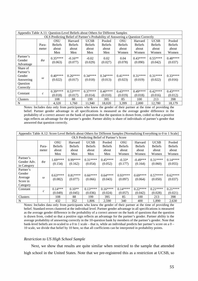
55
Appendix Table A.11: Question-Level Beliefs about Others for Different Samples
OLS Predicting Belief of Partner’s Probability of Answering a Question Correctly
Para-meter
OSU Beliefs about Men
Harvard Beliefs about Men
UCSB Beliefs about Men
Pooled Beliefs about Men
OSU Beliefs about
Women
Harvard Beliefs about
Women
UCSB Beliefs about
Women
Pooled Beliefs about
Women Partner’s Gender Advantage
𝜃𝜃𝜎𝜎 0.35**** (0.063)
-0.16** (0.077)
-0.02 (0.029)
0.02 (0.027)
0.04 (0.078)
0.43**** (0.090)
0.55**** (0.042)
0.48**** (0.037)
Share of Partner’s Gender Answering Question Correctly
𝜔𝜔 0.40**** (0.022)
0.26**** (0.017)
0.34**** (0.018)
0.34**** (0.013)
0.41**** (0.023)
0.31**** (0.019)
0.31**** (0.022)
0.33**** (0.016)
Constant c 0.39**** (0.018)
0.53**** (0.017)
0.37**** (0.014)
0.40**** (0.010)
0.43**** (0.019)
0.49**** (0.018)
0.42**** (0.016)
0.43**** (0.012)
Clusters 108 88 199 395 85 100 213 398 N 4,320 1,760 11,940 18,020 3,399 2,000 12,780 18,179
Notes: Includes data only from participants who knew the gender of their partner at the time of providing the belief. Partner gender advantage in all specifications is measured as the average gender difference in the probability of a correct answer on the bank of questions that the question is drawn from, coded so that a positive sign reflects an advantage for the partner’s gender. Partner ability is share of individuals of partner’s gender that answered that question correctly.
Appendix Table A.12: Score Level Beliefs about Others for Different Samples [Normalizing Everything to 0 to 1 Scale]
OLS Predicting Belief of Partner’s Score
Para-meter
OSU Beliefs about Men
Harvard Beliefs about Men
UCSB Beliefs about Men
Pooled Beliefs about Men
OSU Beliefs about
Women
Harvard Beliefs about
Women
UCSB Beliefs about
Women
Pooled Beliefs about
Women Partner’s Gender Adv. in Category
𝜃𝜃𝜎𝜎 1.69**** (0.154)
0.99**** (0.162)
0.31**** (0.054)
0.45**** (0.052)
-0.33* (0.177)
-0.49*** (0.164)
0.31**** (0.060)
0.14**** (0.055)
Partner’s Gender Average Score in Category
𝜔𝜔 0.63**** (0.082)
0.81**** (0.077)
0.66**** (0.066)
0.64**** (0.043)
0.93**** (0.097)
0.69**** (0.064)
0.57**** (0.050)
0.62**** (0.037)
Constant c 0.14*** (0.049)
0.10** (0.045)
0.13**** (0.036)
0.16**** (0.024)
0.14**** (0.057)
0.22**** (0.042)
0.21**** (0.028)
0.21**** (0.021)
Clusters 108 88 199 395 85 100 213 398 N 432 352 1,806 2,590 340 400 1,890 2,630
Notes: Includes data only from participants who knew the gender of their partner at the time of providing the belief. Standard errors clustered at the individual level. Partner gender advantage in all specifications is measured as the average gender difference in the probability of a correct answer on the bank of questions that the question is drawn from, coded so that a positive sign reflects an advantage for the partner’s gender. Partner ability is the average probability of answering correctly in the 10-question bank by members of the partner’s gender. Note that bank-level beliefs are re-scaled to a 0 to 1 scale – that is, while an individual predicts her partner’s score on a 0 – 10 scale, we divide that belief by 10 here, so that all coefficients can be interpreted in probability points.
Restriction to US High School Sample
Next, we show that results are quite similar when restricted to the sample that attended
high school in the United States. Note that we pre-registered this as a restriction at UCSB, so
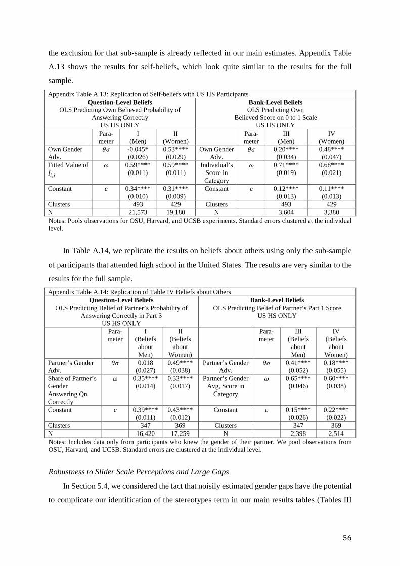
56
the exclusion for that sub-sample is already reflected in our main estimates. Appendix Table
A.13 shows the results for self-beliefs, which look quite similar to the results for the full
sample. Appendix Table A.13: Replication of Self-beliefs with US HS Participants
Question-Level Beliefs OLS Predicting Own Believed Probability of
Answering Correctly US HS ONLY
Bank-Level Beliefs OLS Predicting Own
Believed Score on 0 to 1 Scale US HS ONLY
Para-meter
I (Men)
II (Women)
Para-meter
III (Men)
IV (Women)
Own Gender Adv.
𝜃𝜃𝜎𝜎 -0.045* (0.026)
0.53**** (0.029)
Own Gender Adv.
𝜃𝜃𝜎𝜎 0.20**** (0.034)
0.48**** (0.047)
Fitted Value of 𝐼𝐼𝑖𝑖,𝑗𝑗
𝜔𝜔 0.59**** (0.011)
0.59**** (0.011)
Individual’s Score in Category
𝜔𝜔 0.71**** (0.019)
0.68**** (0.021)
Constant c 0.34**** (0.010)
0.31**** (0.009)
Constant c 0.12**** (0.013)
0.11**** (0.013)
Clusters 493 429 Clusters 493 429 N 21,573 19,180 N 3,604 3,380 Notes: Pools observations for OSU, Harvard, and UCSB experiments. Standard errors clustered at the individual level.
In Table A.14, we replicate the results on beliefs about others using only the sub-sample
of participants that attended high school in the United States. The results are very similar to the
results for the full sample. Appendix Table A.14: Replication of Table IV Beliefs about Others
Question-Level Beliefs OLS Predicting Belief of Partner’s Probability of
Answering Correctly in Part 3 US HS ONLY
Bank-Level Beliefs OLS Predicting Belief of Partner’s Part 1 Score
US HS ONLY
Para-meter
I (Beliefs about Men)
II (Beliefs about
Women)
Para-meter
III (Beliefs about Men)
IV (Beliefs about
Women) Partner’s Gender Adv.
𝜃𝜃𝜎𝜎 0.018 (0.027)
0.49**** (0.038)
Partner’s Gender Adv.
𝜃𝜃𝜎𝜎 0.41**** (0.052)
0.18**** (0.055)
Share of Partner’s Gender Answering Qn. Correctly
𝜔𝜔 0.35**** (0.014)
0.32**** (0.017)
Partner’s Gender Avg, Score in
Category
𝜔𝜔 0.65**** (0.046)
0.60**** (0.038)
Constant c 0.39**** (0.011)
0.43**** (0.012)
Constant c 0.15**** (0.026)
0.22**** (0.022)
Clusters 347 369 Clusters 347 369 N 16,420 17,259 N 2,398 2,514 Notes: Includes data only from participants who knew the gender of their partner. We pool observations from OSU, Harvard, and UCSB. Standard errors are clustered at the individual level.
Robustness to Slider Scale Perceptions and Large Gaps
In Section 5.4, we considered the fact that noisily estimated gender gaps have the potential
to complicate our identification of the stereotypes term in our main results tables (Tables III
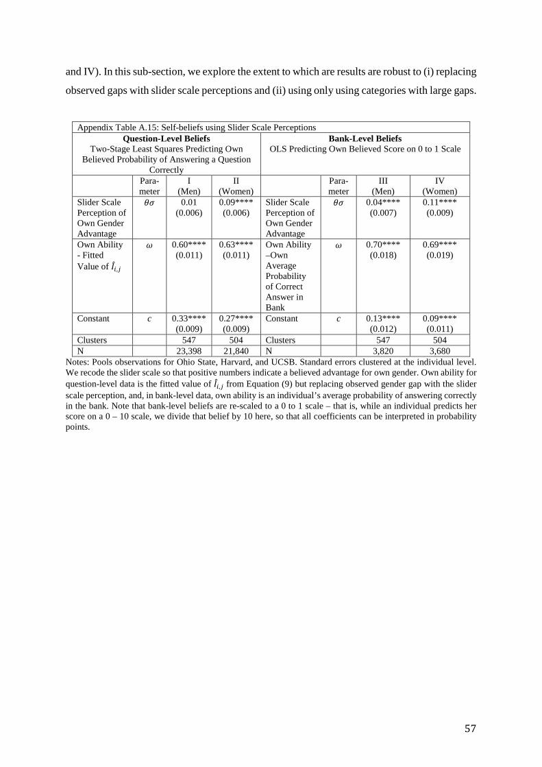
57
and IV). In this sub-section, we explore the extent to which are results are robust to (i) replacing
observed gaps with slider scale perceptions and (ii) using only using categories with large gaps.
Appendix Table A.15: Self-beliefs using Slider Scale Perceptions
Question-Level Beliefs Two-Stage Least Squares Predicting Own
Believed Probability of Answering a Question Correctly
Bank-Level Beliefs OLS Predicting Own Believed Score on 0 to 1 Scale
Para-meter
I (Men)
II (Women)
Para-meter
III (Men)
IV (Women)
Slider Scale Perception of Own Gender Advantage
𝜃𝜃𝜎𝜎 0.01 (0.006)
0.09**** (0.006)
Slider Scale Perception of Own Gender Advantage
𝜃𝜃𝜎𝜎 0.04**** (0.007)
0.11**** (0.009)
Own Ability - Fitted Value of 𝐼𝐼𝑖𝑖,𝑗𝑗
𝜔𝜔 0.60**** (0.011)
0.63**** (0.011)
Own Ability –Own Average Probability of Correct Answer in Bank
𝜔𝜔 0.70**** (0.018)
0.69**** (0.019)
Constant c 0.33**** (0.009)
0.27**** (0.009)
Constant c 0.13**** (0.012)
0.09**** (0.011)
Clusters 547 504 Clusters 547 504 N 23,398 21,840 N 3,820 3,680
Notes: Pools observations for Ohio State, Harvard, and UCSB. Standard errors clustered at the individual level. We recode the slider scale so that positive numbers indicate a believed advantage for own gender. Own ability for question-level data is the fitted value of 𝐼𝐼𝑖𝑖,𝑗𝑗 from Equation (9) but replacing observed gender gap with the slider scale perception, and, in bank-level data, own ability is an individual’s average probability of answering correctly in the bank. Note that bank-level beliefs are re-scaled to a 0 to 1 scale – that is, while an individual predicts her score on a 0 – 10 scale, we divide that belief by 10 here, so that all coefficients can be interpreted in probability points.
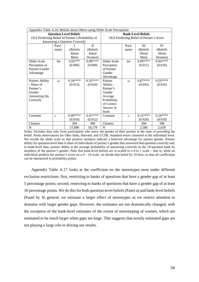
58
Appendix Table A.16: Beliefs about Others using Slider Scale Perceptions
Question-Level Beliefs OLS Predicting Belief of Partner’s Probability of
Answering a Question Correctly
Bank-Level Beliefs OLS Predicting Belief of Partner’s Score
Para-meter
I (Beliefs About Men)
II (Beliefs About
Women)
Para-meter
III (Beliefs About Men)
IV (Beliefs About
Women) Slider Scale Perception of Partner Gender Advantage
𝜃𝜃𝜎𝜎 0.02*** (0.006)
0.08**** (0.009)
Slider Scale Perception of Partner Gender Advantage
𝜃𝜃𝜎𝜎 0.09**** (0.011)
0.06**** (0.010)
Partner Ability - Share of Partner’s Gender Answering Qn. Correctly
𝜔𝜔 0.34**** (0.013)
0.35**** (0.016)
Partner Ability - Partner’s Gender Average Probability of Correct Answer in Bank
𝜔𝜔 0.67**** (0.043)
0.55**** (0.035)
Constant c 0.40**** (0.010)
0.41**** (0.012)
Constant c 0.15**** (0.024)
0.24**** (0.018)
Clusters 394 398 Clusters 394 398 N 17,890 18,179 N 2,586 2,630
Notes: Includes data only from participants who knew the gender of their partner at the time of providing the belief. Pools observations for Ohio State, Harvard, and UCSB. Standard errors clustered at the individual level. We recode the slider scale so that positive numbers indicate a believed advantage for partner gender. Partner ability for question-level data is share of individuals of partner’s gender that answered that question correctly and, in bank-level data, partner ability is the average probability of answering correctly in the 10-question bank by members of the partner’s gender. Note that bank-level beliefs are re-scaled to a 0 to 1 scale – that is, while an individual predicts her partner’s score on a 0 – 10 scale, we divide that belief by 10 here, so that all coefficients can be interpreted in probability points.
Appendix Table A.17 looks at the coefficient on the stereotypes term under different
exclusion restrictions: first, restricting to banks of questions that have a gender gap of at least
5 percentage points; second, restricting to banks of questions that have a gender gap of at least
10 percentage points. We do this for both question-level beliefs (Panel a) and bank-level beliefs
(Panel b). In general, we estimate a larger effect of stereotypes as we restrict attention to
domains with larger gender gaps. However, the estimates are not dramatically changed, with
the exception of the bank-level estimates of the extent of stereotyping of women, which are
estimated to be much larger when gaps are large. This suggests that noisily estimated gaps are
not playing a large role in driving our results.
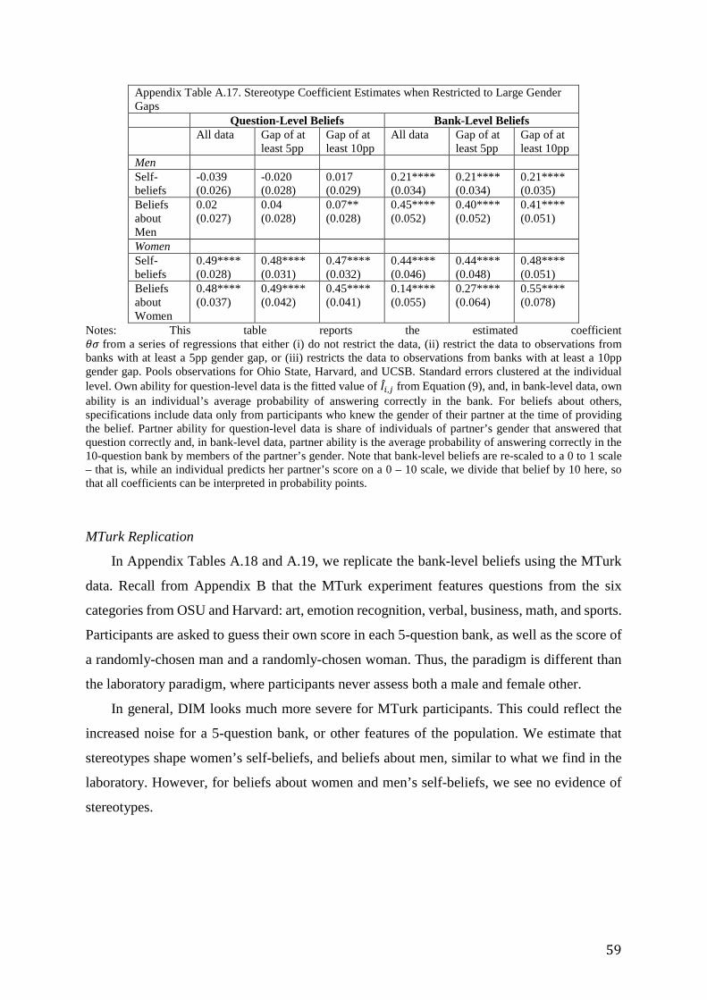
59
Appendix Table A.17. Stereotype Coefficient Estimates when Restricted to Large Gender Gaps Question-Level Beliefs Bank-Level Beliefs All data Gap of at
least 5pp Gap of at least 10pp
All data Gap of at least 5pp
Gap of at least 10pp
Men Self-beliefs
-0.039 (0.026)
-0.020 (0.028)
0.017 (0.029)
0.21**** (0.034)
0.21**** (0.034)
0.21**** (0.035)
Beliefs about Men
0.02 (0.027)
0.04 (0.028)
0.07** (0.028)
0.45**** (0.052)
0.40**** (0.052)
0.41**** (0.051)
Women Self-beliefs
0.49**** (0.028)
0.48**** (0.031)
0.47**** (0.032)
0.44**** (0.046)
0.44**** (0.048)
0.48**** (0.051)
Beliefs about Women
0.48**** (0.037)
0.49**** (0.042)
0.45**** (0.041)
0.14**** (0.055)
0.27**** (0.064)
0.55**** (0.078)
Notes: This table reports the estimated coefficient 𝜃𝜃𝜎𝜎 from a series of regressions that either (i) do not restrict the data, (ii) restrict the data to observations from banks with at least a 5pp gender gap, or (iii) restricts the data to observations from banks with at least a 10pp gender gap. Pools observations for Ohio State, Harvard, and UCSB. Standard errors clustered at the individual level. Own ability for question-level data is the fitted value of 𝐼𝐼𝑖𝑖,𝑗𝑗 from Equation (9), and, in bank-level data, own ability is an individual’s average probability of answering correctly in the bank. For beliefs about others, specifications include data only from participants who knew the gender of their partner at the time of providing the belief. Partner ability for question-level data is share of individuals of partner’s gender that answered that question correctly and, in bank-level data, partner ability is the average probability of answering correctly in the 10-question bank by members of the partner’s gender. Note that bank-level beliefs are re-scaled to a 0 to 1 scale – that is, while an individual predicts her partner’s score on a 0 – 10 scale, we divide that belief by 10 here, so that all coefficients can be interpreted in probability points.
MTurk Replication
In Appendix Tables A.18 and A.19, we replicate the bank-level beliefs using the MTurk
data. Recall from Appendix B that the MTurk experiment features questions from the six
categories from OSU and Harvard: art, emotion recognition, verbal, business, math, and sports.
Participants are asked to guess their own score in each 5-question bank, as well as the score of
a randomly-chosen man and a randomly-chosen woman. Thus, the paradigm is different than
the laboratory paradigm, where participants never assess both a male and female other.
In general, DIM looks much more severe for MTurk participants. This could reflect the
increased noise for a 5-question bank, or other features of the population. We estimate that
stereotypes shape women’s self-beliefs, and beliefs about men, similar to what we find in the
laboratory. However, for beliefs about women and men’s self-beliefs, we see no evidence of
stereotypes.
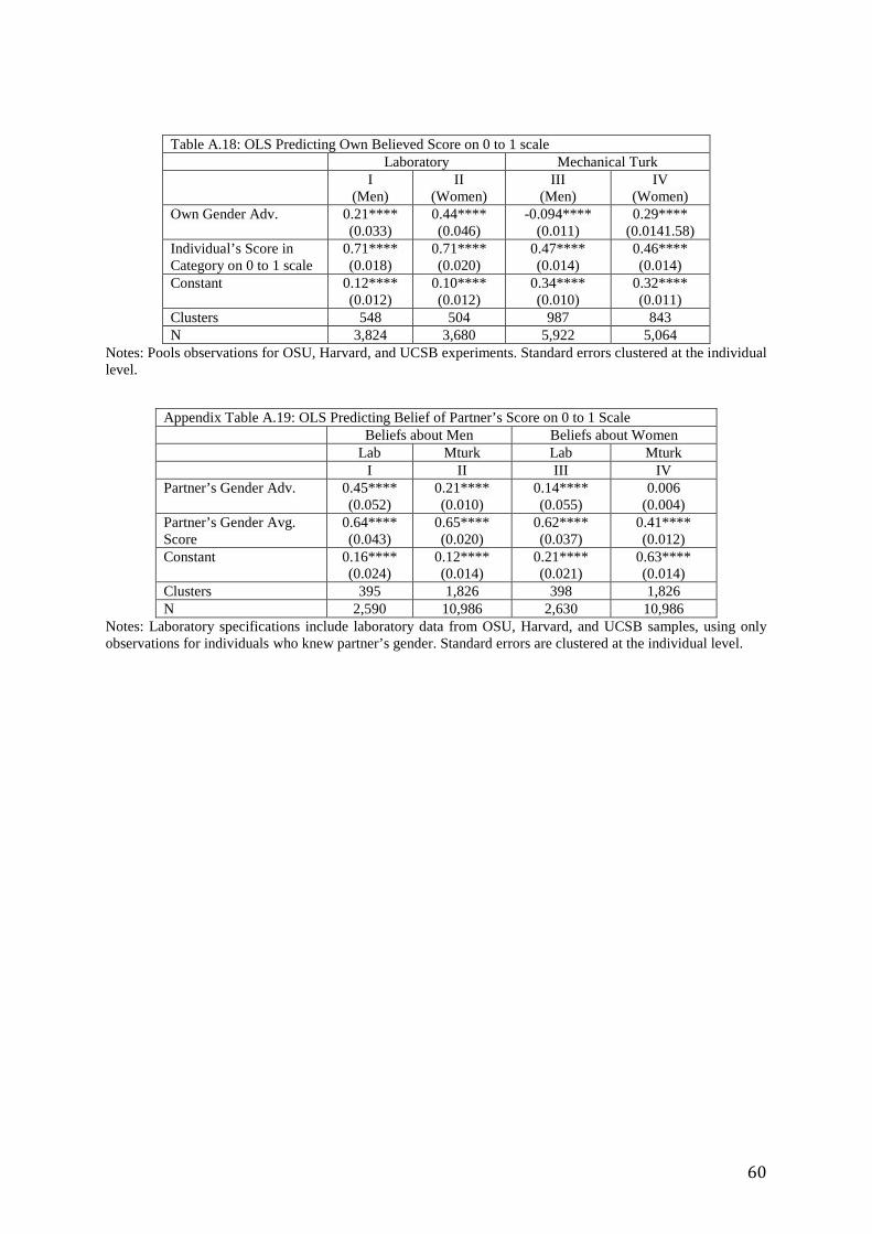
60
Table A.18: OLS Predicting Own Believed Score on 0 to 1 scale Laboratory Mechanical Turk I
(Men) II
(Women) III
(Men) IV
(Women) Own Gender Adv. 0.21****
(0.033) 0.44**** (0.046)
-0.094**** (0.011)
0.29**** (0.0141.58)
Individual’s Score in Category on 0 to 1 scale
0.71**** (0.018)
0.71**** (0.020)
0.47**** (0.014)
0.46**** (0.014)
Constant 0.12**** (0.012)
0.10**** (0.012)
0.34**** (0.010)
0.32**** (0.011)
Clusters 548 504 987 843 N 3,824 3,680 5,922 5,064
Notes: Pools observations for OSU, Harvard, and UCSB experiments. Standard errors clustered at the individual level.
Appendix Table A.19: OLS Predicting Belief of Partner’s Score on 0 to 1 Scale Beliefs about Men Beliefs about Women Lab Mturk Lab Mturk I II III IV Partner’s Gender Adv. 0.45****
(0.052) 0.21**** (0.010)
0.14**** (0.055)
0.006 (0.004)
Partner’s Gender Avg. Score
0.64**** (0.043)
0.65**** (0.020)
0.62**** (0.037)
0.41**** (0.012)
Constant 0.16**** (0.024)
0.12**** (0.014)
0.21**** (0.021)
0.63**** (0.014)
Clusters 395 1,826 398 1,826 N 2,590 10,986 2,630 10,986
Notes: Laboratory specifications include laboratory data from OSU, Harvard, and UCSB samples, using only observations for individuals who knew partner’s gender. Standard errors are clustered at the individual level.


![BELIEFS ABOUT BRILLIANCE UNDERMINE THE CAREERS OF …wc.uchicago.edu/files/2016/04/Beliefs-about-Brilliance-Poster1.pdf · Beliefs about Brilliance Poster v3_FINAL[2] Author: Mary](https://img.pdfslide.net/doc/110x75/5f3136c6074227538e773ebc/beliefs-about-brilliance-undermine-the-careers-of-wc-beliefs-about-brilliance-poster.jpg)