Embed Size (px)
DESCRIPTION
Very useful when dealing with atmospheric fluid dynamics
Citation preview
Meteorological Training Course Lecture Series
ECMWF, 2002 1
The parametrization of the planetary boundarylayerMay 1992
By Anton Beljaars
European Centre for Medium-Range Weather Forecasts
Table of contents
1 . Introduction
1.1 The planetary boundary layer
1.2 Importance of the PBL in large-scale models
1.3 Recommended literature
1.4 General characteristics of the planetary boundary layer
1.5 Conserved quantities and static stability
1.6 Basic equations
1.7 Ekman equation
2 . Similarity theory and surface fluxes
2.1 Surface-layer similarity
2.2 The outer layer
2.3 Matching of surface and outer layer (drag laws)
2.4 Surface boundary conditions and surface fluxes
3 . PBL schemes for atmospheric models
3.1 Geostrophic transfer laws
3.2 Integral models (slab, bulk models)
3.3 Grid point models with�
-closure
3.4�
-profile closures
3.5 TKE-closure
4 . List of symbols
REFERENCES
The parametrization of the planetary boundary layer
2 Meteorological Training Course Lecture Series
ECMWF, 2002
1. INTRODUCTION
1.1 The planetary boundary layer
Theplanetaryboundarylayer (PBL) is the region of theatmospherenearthesurfacewherethe influenceof the
surfaceis felt throughturbulent exchangeof momentum,heatandmoisture.The equationswhich describethe
large-scaleevolutionof theatmospheredonottakeinto accounttheinteractionwith thesurface.Theturbulentmo-
tion responsible for this interaction is small-scale and totally sub-grid and therefore needs to be parametrized.
Thetransitionregionbetweenthesurfaceandthefreeatmosphere,whereverticaldiffusiondueto turbulentmotion
takesplace,variesin depth.ThePBL canbeasshallow as100m duringnightoverlandandgoupto afew thousand
metreswhentheatmosphereis heatedfrom thesurface.ThePBL parametrizationdeterminestogetherwith thesur-
faceparametrizationthesurfacefluxesandredistributesthesurfacefluxesovertheboundarylayerdepth.Boundary
layerprocessesarerelatively quick; thePBL respondsto its forcing within a few hourswhich is fastcomparedto
thetimescaleof thelarge-scaleevolutionof theatmosphere,in otherwords:thePBL isalwaysin quasi-equilibrium
with the large-scale forcing.
1.2 Importance of the PBL in large-scale models
A number of reasons exists to have a realistic representation of the boundary layer in a large scale model:
• The large-scalebudgetsof momentumheatandmoistureareconsiderablyaffectedby the surface
fluxes on time scales of a few days.
• Model variables in the boundary layer are important model products.
• The boundary layer interacts with other processes e.g. clouds and convection.
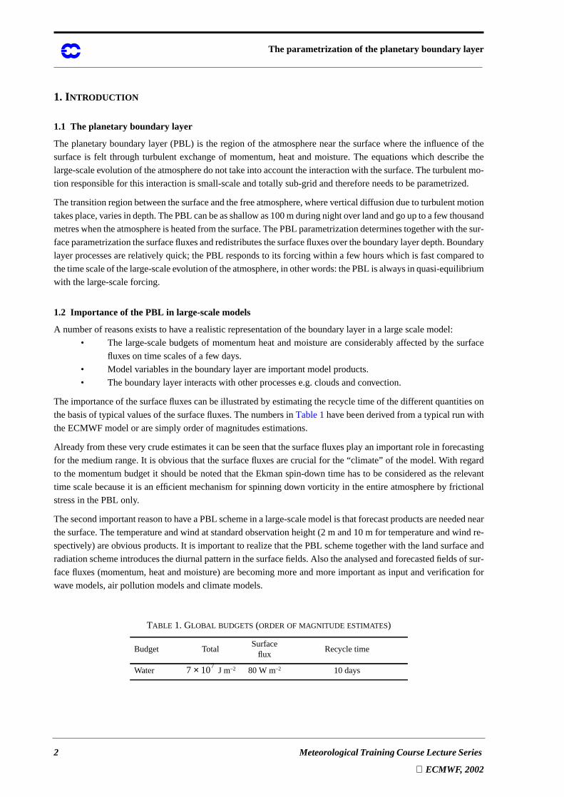
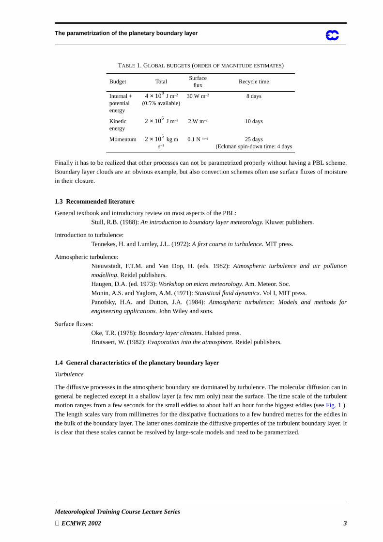
Theimportanceof thesurfacefluxescanbeillustratedby estimatingtherecycle timeof thedifferentquantitieson
thebasisof typicalvaluesof thesurfacefluxes.Thenumbersin Table1 havebeenderivedfrom atypical runwith
the ECMWF model or are simply order of magnitudes estimations.
Alreadyfrom theseverycrudeestimatesit canbeseenthatthesurfacefluxesplayanimportantrole in forecasting
for themediumrange.It is obviousthatthesurfacefluxesarecrucial for the“climate” of themodel.With regard
to themomentumbudgetit shouldbenotedthat theEkmanspin-down time hasto beconsideredastherelevant
time scalebecauseit is anefficient mechanismfor spinningdown vorticity in theentireatmosphereby frictional
stress in the PBL only.
Thesecondimportantreasonto haveaPBL schemein alarge-scalemodelis thatforecastproductsareneedednear
thesurface.Thetemperatureandwind atstandardobservationheight(2 m and10m for temperatureandwind re-
spectively) areobviousproducts.It is importantto realizethatthePBL schemetogetherwith thelandsurfaceand
radiationschemeintroducesthediurnalpatternin thesurfacefields.Also theanalysedandforecastedfieldsof sur-
facefluxes(momentum,heatandmoisture)arebecomingmoreandmoreimportantasinput andverificationfor
wave models, air pollution models and climate models.
TABLE 1. GLOBAL BUDGETS(ORDEROF MAGNITUDE ESTIMATES)
Budget TotalSurface
fluxRecycle time
Water J m–2 80 W m–2 10 days7 107×
The parametrization of the planetary boundary layer
Meteorological Training Course Lecture Series
ECMWF, 2002 3
Finally it hasto berealizedthatotherprocessescannot beparametrizedproperlywithout having a PBL scheme.
Boundarylayercloudsareanobviousexample,but alsoconvectionschemesoftenusesurfacefluxesof moisture
in their closure.
1.3 Recommended literature
General textbook and introductory review on most aspects of the PBL:
Stull, R.B. (1988):An introduction to boundary layer meteorology. Kluwer publishers.
Introduction to turbulence:
Tennekes, H. and Lumley, J.L. (1972):A first course in turbulence. MIT press.
Atmospheric turbulence:
Nieuwstadt,F.T.M. and Van Dop, H. (eds. 1982): Atmosphericturbulence and air pollution
modelling. Reidel publishers.
Haugen, D.A. (ed. 1973):Workshop on micro meteorology. Am. Meteor. Soc.
Monin, A.S. and Yaglom, A.M. (1971):Statistical fluid dynamics. Vol I, MIT press.
Panofsky, H.A. and Dutton, J.A. (1984): Atmosphericturbulence: Models and methodsfor
engineering applications. John Wiley and sons.
Surface fluxes:
Oke, T.R. (1978):Boundary layer climates. Halsted press.
Brutsaert, W. (1982):Evaporation into the atmosphere. Reidel publishers.
1.4 General characteristics of the planetary boundary layer
Turbulence
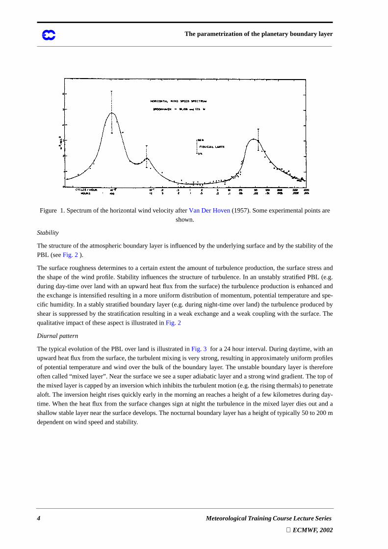
Thediffusiveprocessesin theatmosphericboundaryaredominatedby turbulence.Themoleculardiffusioncanin
generalbeneglectedexceptin a shallow layer (a few mm only) nearthesurface.Thetime scaleof the turbulent
motionrangesfrom a few secondsfor thesmalleddiesto abouthalf anhour for thebiggesteddies(seeFig. 1 ).
Thelengthscalesvary from millimetresfor thedissipative fluctuationsto a few hundredmetresfor theeddiesin
thebulk of theboundarylayer. Thelatteronesdominatethediffusivepropertiesof theturbulentboundarylayer. It
is clear that these scales cannot be resolved by large-scale models and need to be parametrized.
Internal +potentialenergy
J m–2
(0.5%available)30 W m–2 8 days
Kineticenergy
J m–2 2 W m–2 10 days
Momentum kg ms–1
0.1 Nm–2 25 days(Eckman spin-down time: 4 days
TABLE 1. GLOBAL BUDGETS(ORDEROF MAGNITUDE ESTIMATES)
Budget TotalSurface
fluxRecycle time
4 109×
2 106×
2 105×
The parametrization of the planetary boundary layer
4 Meteorological Training Course Lecture Series
ECMWF, 2002
Figure 1. Spectrum of the horizontal wind velocity afterVan Der Hoven (1957). Some experimental points are
shown.
Stability
Thestructureof theatmosphericboundarylayeris influencedby theunderlyingsurfaceandby thestabilityof the
PBL (seeFig. 2).
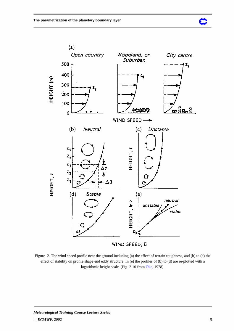
Thesurfaceroughnessdeterminesto a certainextent theamountof turbulenceproduction,thesurfacestressand
theshapeof thewind profile. Stability influencesthestructureof turbulence.In anunstablystratifiedPBL (e.g.
duringday-timeover landwith anupwardheatflux from thesurface)theturbulenceproductionis enhancedand
theexchangeis intensifiedresultingin a moreuniform distribution of momentum,potentialtemperatureandspe-
cific humidity. In a stablystratifiedboundarylayer(e.g.duringnight-timeover land)theturbulenceproducedby
shearis suppressedby thestratificationresultingin a weakexchangeanda weakcouplingwith thesurface.The
qualitative impact of these aspect is illustrated inFig. 2
Diurnal pattern
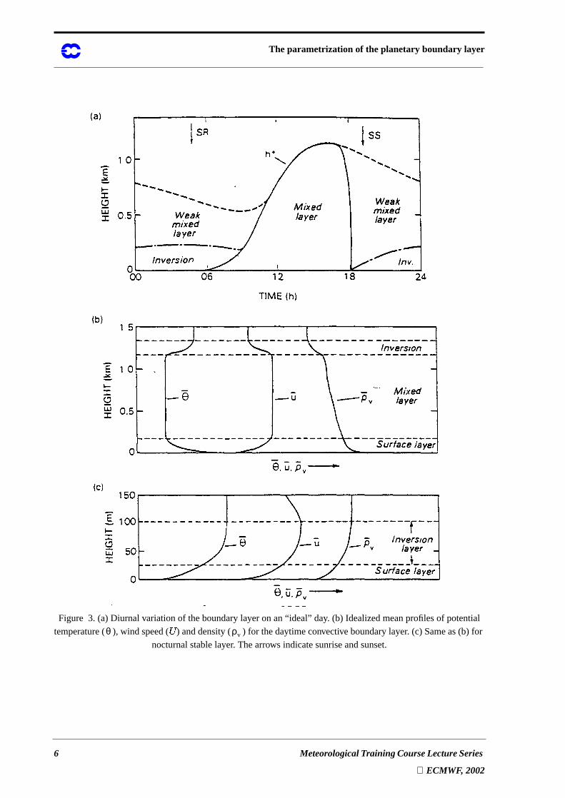
Thetypical evolution of thePBL over landis illustratedin Fig. 3 for a 24 hourinterval. During daytime,with an
upwardheatflux from thesurface,theturbulentmixing is verystrong,resultingin approximatelyuniformprofiles
of potentialtemperatureandwind over thebulk of theboundarylayer. Theunstableboundarylayer is therefore
oftencalled“mixedlayer”. Nearthesurfaceweseeasuperadiabaticlayerandastrongwind gradient.Thetopof
themixedlayeris cappedby aninversionwhichinhibits theturbulentmotion(e.g.therisingthermals)to penetrate
aloft. Theinversionheightrisesquickly early in themorninganreachesa heightof a few kilometresduringday-
time. Whentheheatflux from thesurfacechangessignat night the turbulencein themixed layerdiesout anda
shallow stablelayernearthesurfacedevelops.Thenocturnalboundarylayerhasaheightof typically 50 to 200m
dependent on wind speed and stability.
The parametrization of the planetary boundary layer
Meteorological Training Course Lecture Series
ECMWF, 2002 5
Figure 2. The wind speed profile near the ground including (a) the effect of terrain roughness, and (b) to (e) the
effect of stability on profile shape end eddy structure. In (e) the profiles of (b) to (d) are re-plotted with a
logarithmic height scale. (Fig. 2.10 fromOke, 1978).
The parametrization of the planetary boundary layer
6 Meteorological Training Course Lecture Series
ECMWF, 2002
Figure 3. (a) Diurnal variation of the boundary layer on an “ideal” day. (b) Idealized mean profiles of potential
temperature( ), wind speed( � ) anddensity( ) for thedaytimeconvectiveboundarylayer. (c) Sameas(b) for
nocturnal stable layer. The arrows indicate sunrise and sunset.
θ ρv
The parametrization of the planetary boundary layer
Meteorological Training Course Lecture Series
ECMWF, 2002 7
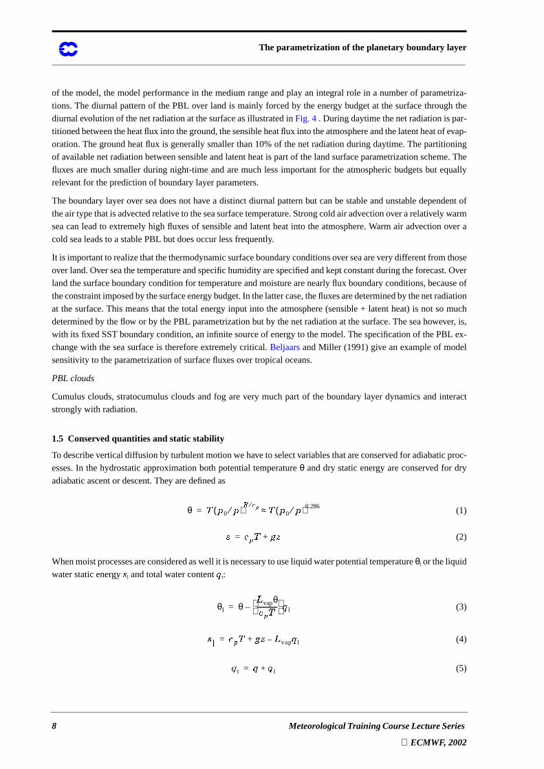
Surface fluxes
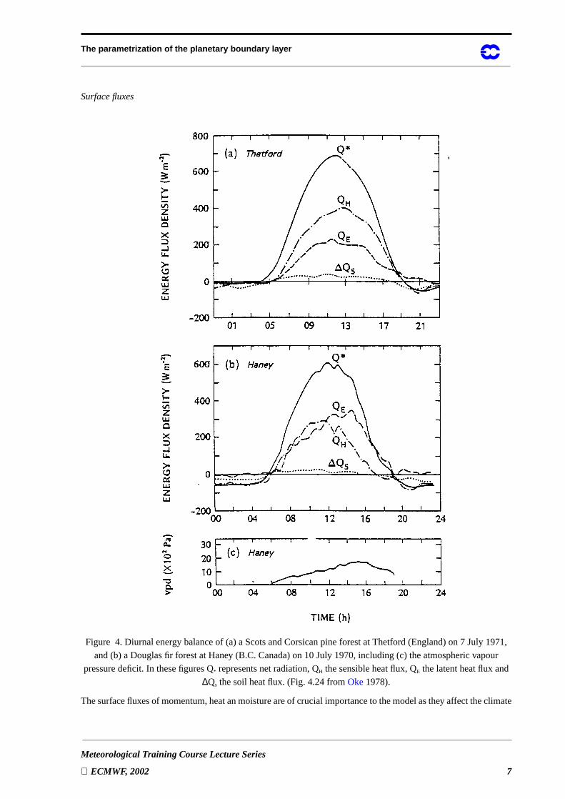
Figure 4. Diurnal energy balance of (a) a Scots and Corsican pine forest at Thetford (England) on 7 July 1971,
and (b) a Douglas fir forest at Haney (B.C. Canada) on 10 July 1970, including (c) the atmospheric vapour
pressure deficit. In these figures Q* represents net radiation, QH the sensible heat flux, QE the latent heat flux and
∆Qs the soil heat flux. (Fig. 4.24 fromOke 1978).
Thesurfacefluxesof momentum,heatanmoistureareof crucialimportanceto themodelasthey affect theclimate
The parametrization of the planetary boundary layer
8 Meteorological Training Course Lecture Series
ECMWF, 2002
of themodel,themodelperformancein themediumrangeandplay an integral role in a numberof parametriza-
tions.Thediurnalpatternof thePBL over land is mainly forcedby theenergy budgetat thesurfacethroughthe
diurnalevolutionof thenetradiationat thesurfaceasillustratedin Fig. 4 . Duringdaytimethenetradiationis par-
titionedbetweentheheatflux into theground,thesensibleheatflux into theatmosphereandthelatentheatof evap-
oration.Thegroundheatflux is generallysmallerthan10%of thenetradiationduringdaytime.Thepartitioning
of availablenetradiationbetweensensibleandlatentheatis partof thelandsurfaceparametrizationscheme.The
fluxesaremuchsmallerduring night-timeandaremuchlessimportantfor the atmosphericbudgetsbut equally
relevant for the prediction of boundary layer parameters.
Theboundarylayerover seadoesnot have a distinctdiurnalpatternbut canbestableandunstabledependentof
theair typethatis advectedrelativeto theseasurfacetemperature.Strongcoldair advectionoverarelatively warm
seacanleadto extremelyhigh fluxesof sensibleandlatentheatinto theatmosphere.Warmair advectionover a
cold sea leads to a stable PBL but does occur less frequently.
It is importantto realizethatthethermodynamicsurfaceboundaryconditionsoverseaareverydifferentfrom those
over land.Overseathetemperatureandspecifichumidityarespecifiedandkeptconstantduringtheforecast.Over
landthesurfaceboundaryconditionfor temperatureandmoisturearenearlyflux boundaryconditions,becauseof
theconstraintimposedby thesurfaceenergybudget.In thelattercase,thefluxesaredeterminedby thenetradiation
at thesurface.This meansthat the total energy input into theatmosphere(sensible+ latentheat)is not somuch
determinedby theflow or by thePBL parametrizationbut by thenetradiationat thesurface.Theseahowever, is,
with its fixedSSTboundarycondition,aninfinite sourceof energy to themodel.Thespecificationof thePBL ex-
changewith theseasurfaceis thereforeextremelycritical. BeljaarsandMiller (1991)give anexampleof model
sensitivity to the parametrization of surface fluxes over tropical oceans.
PBL clouds
Cumulusclouds,stratocumuluscloudsandfog arevery muchpart of the boundarylayer dynamicsandinteract
strongly with radiation.
1.5 Conserved quantities and static stability
To describeverticaldiffusionby turbulentmotionwehaveto selectvariablesthatareconservedfor adiabaticproc-
esses.In thehydrostaticapproximationbothpotentialtemperatureθ anddry staticenergy areconserved for dry
adiabatic ascent or descent. They are defined as
(1)
(2)
Whenmoistprocessesareconsideredaswell it is necessaryto useliquid waterpotentialtemperatureθl or theliquid
water static energy � l and total water content� t:
(3)
(4)
(5)
θ ��� 0 �⁄( )���
⁄ ��� 0 �⁄( )0.286≈=
� �� � ���+=
θl θ�
vap� �-------------
� l–=
� l �� � ��� �vap � l–+=
� t � � l+=
The parametrization of the planetary boundary layer
Meteorological Training Course Lecture Series
ECMWF, 2002 9
Thestaticstability is determinedby thedensityof afluid parcelmovedadiabaticallyto a referenceheightin com-
parisonwith thedensityof thesurroundingfluid. Thevirtual potentialtemperatureθv andthevirtual dry staticen-
ergy are often used for this purpose:
(6)
(7)
1.6 Basic equations
To illustratetheclosureproblemwederivetheReynoldsequationsfor momentum,startingfrom thethreemomen-
tumequationsfor incompressibleflow in arectangularcoordinatesystemwith z perpendicularto theearthsurface:
(8)
(9)
Decomposition of each variable into a mean part and a fluctuating (turbulent) part:
(10)
After averaging,applicationof theBoussinesqapproximation(retaindensityfluctuationsin thebuoyancy terms
only) and applying the hydrostatic approximation:
(11)
(12)
Furthersimplificationsareobtainedby neglectingviscouseffectsfor largeReynoldsnumbers( � � /ν >> 1, where�is a lengthscale)andby assumingthatthe����� -scalesaremuchlargerthanthe� -scales(boundarylayerapprox-
imation):
θv θ 1
�v�------- 1–
� � l–+ θ 1 0.61� � l–+{ }= =
� v �� � 1 0.61� � l–+{ } ���+=
∂ �∂ �------ � ∂ �
∂�------ � ∂ �∂�------ � ∂ �
∂�------ � �–+ + + =1ρ---∂�
∂�------– ν∇2 �+
∂ �∂ �------ � ∂ �
∂�------ � ∂ �∂�------ � ∂ �
∂�------ � �+ + + + =1ρ---∂�
∂�------– ν∇2 �+
∂ �∂ �------- � ∂ �
∂�------- � ∂ �∂�------- � ∂ �
∂�-------+ + + =1ρ---∂�
∂�------– ν∇ � �–+
∂ �∂�------ ∂ �
∂�------ ∂ �∂�-------+ + 0=
� � � ′ , ρ+ ρ0 ρ′ ,+= =
� ! � ′ , �+ " � ′ ,+= =
� # � ′+=
∂ �∂ �-------- � ∂ �
∂�-------- ! ∂ �∂�-------- # ∂ �
∂�-------- � !–+ + + =1ρ0-----∂"
∂�-------– ν∇2 � ∂∂�------ � ′ � ′ ∂
∂�------ � ′ � ′–∂
∂�------ � ′ � ′––+
∂ !∂ �------- � ∂ !
∂�------- ! ∂ !∂�------- # ∂ !
∂�------- � �+ + + + =1ρ0-----∂"
∂�-------– ν∇2 ! ∂∂�------ � ′ � ′ ∂
∂�------ � ′ � ′–∂
∂�------ � ′ � ′––+
� =1ρ0-----∂"
∂�-------–
∂ �∂�-------- ∂ !
∂�------- ∂ #∂�---------+ + 0=
The parametrization of the planetary boundary layer
10 Meteorological Training Course Lecture Series
ECMWF, 2002
(13)
Theseequationsdescribethehorizontalmomentumbudgetof the resolvedflow andhave extra termsdueto the
Reynoldsdecompositionandaveragingprocedure.Theterms and areknown astheReynoldsstresses
andrepresentverticaltransportof horizontalmomentumby unresolvedturbulentmotion.Thesearethetermsthat
need to be parametrized. Similar equations exist for potential temperature and specific humidity.
An equationthatis importantin someparametrizationschemesandgivesinsightin thedynamicsof turbulenceis
theequationfor turbulentkineticenergy. To derive it, theequationsfor thefluctuatingquantitiesaretakenby sub-
tractingtheequationsfor meanmomentumfrom theequationsfor totalmomentum.Thekineticenergy of thefluc-
tuationsis obtainedby multiplying theequationsfor thedifferentcomponentsby thevelocityfluctuationitself and
by adding the three equations for the three components. The result is:
(14)
(15)
Theleft handsideof thisequationrepresentstimedependenceandadvection.Theright handsidehassource,sink
andtransportterms.TermsI representmechanicalproductionof turbulenceby wind shearandconvert energy of
themeanflow into turbulence.Termtwo is theproductionof turbulenceby buoyancy andconvertspotentialenergy
of theatmosphereto turbulenceor vice versa.TermsIII andIV aretransportor turbulentdiffusiontermsbecause
they equalzerowhenvertically integratedover thedomain.They representtheverticaltransportof turbulenceen-
ergyby theturbulentfluctuationsandthepressurefluctuationsrespectively. Thelastterm(V) is thedissipationterm
which converts turbulence kinetic energy into heat by molecular friction at very small scales.
1.7 Ekman equation
To illustratethemechanismof Ekmanpumpingweconsiderthefollowing equationsfor thesteadystateboundary
layer:
(16)
(17)
∂ �∂ �-------- � ∂ �
∂�-------- ! ∂ �∂�-------- # ∂ �
∂�-------- � !–+ + +1ρ0-----∂"
∂�-------– ∂ � ′ � ′∂�---------------–=
∂ !∂ �------- � ∂ !
∂�------- ! ∂ !∂�------- # ∂ !
∂�------- � �+ + + +1ρ0-----∂"
∂�------- ∂ � ′ � ′∂�---------------––=
� 1ρ0-----∂"
∂�-------–=
� ′ � ′ � ′ � ′
$′ � ′
$ 12--- � ′2 � ′2 � ′2+ +( )=
∂$
∂ �------- � ∂$
∂�------- ! ∂$
∂�------- # ∂$
∂�-------+ + + = � ′ � ′∂ �∂�--------– � ′ � ′∂ !∂�-------–�ρ0----- � ′ρ′–
I I II
+∂
∂�------$
′ � ′ +
� ′ � ′ρ
------------ ε–
III IV V
�%! ! G–( )–∂ � ′ � ′
∂�--------------- where �&! G,–1ρ0-----∂"
∂�-------= =
� � � G–( )–∂ � ′ � ′
∂�--------------- where � � G,– 1ρ0-----–
∂"∂�-------= =
The parametrization of the planetary boundary layer
Meteorological Training Course Lecture Series
ECMWF, 2002 11
For a simpleclosurewith , andconstant' we rewrite theequationsin
complex notation:
(18)
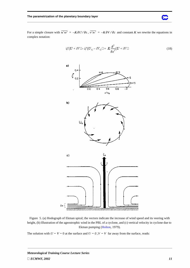
Figure 5. (a) Hodograph of Ekman spiral; the vectors indicate the increase of wind speed and its veering with
height,(b) Illustrationof theageostrophicwind in thePBL of acyclone,and(c) verticalvelocity in cyclonedueto
Ekman pumping (Holton, 1979).
The solution with�%( ! ( 0 at the surface and�%()� ,! ( ! far away from the surface, reads:
� ′ � ′ ' ∂ � ∂�⁄–= � ′ � ′ ' ∂ ! ∂�⁄–=
i � � i !+( ) * � � G i ! G–( )– ' ∂2
∂� 2-------- � i !+( )=
The parametrization of the planetary boundary layer
12 Meteorological Training Course Lecture Series
ECMWF, 2002
(19)
Theverticalvelocity #,+ at thetopof thePBL is derivedfrom thecontinuityequationby integrationfrom thesur-
face to boundary layer depth- , where- is large.
(20)
Weseethattheverticalvelocityat thetopof thePBL is proportionalto thecurl of thesurfacestressandto thecurl
of thegeostrophicwind. This qualitative resultis in fact independentof how ' is exactly specified.Thevertical
velocity canbeeseenasa boundaryconditionfor theinviscid flow above theboundarylayer. Theinflow of air in
acyclonedueto friction at thesurfacecausesanascendingmotionat thetopof thePBL andspinsdown thevortex
by vortex compression(conservationof angularmomentum).This mechanismis very importantbecauseit trans-
fers the effect of boundary layer friction to the entire troposphere. Ekman pumping is illustrated inFig. 5.
2. SIMILARITY THEORY AND SURFACE FLUXES
Many physicalprocessesin theatmospherearetoocomplicatedto enablethederivationof parametrizationsonthe
basisof first principles.Turbulenceis suchanexample:althoughturbulentfluctuationsaredescribedby theequa-
tionsof motionfor acontinuumfluid, it is verydifficult to generatesolutionsof theseequationsandmoreover the
solutionsshow chaoticbehaviour on very shorttime scales.Most of thetime we areonly interestedin statistical
averages.It is thereforecommonpracticeto rely onempiricalrelationshipsbasedonobservations.Similarity the-
ory provides the framework to organize and group the experimental data.
Similarity theorystartswith theidentificationof therelevantphysicalparameters,thendimensionlessgroupsare
formedfrom thetheseparameters,andfinally experimentaldatais usedto find functionalrelationsbetweendimen-
sionlessgroups.Whenthefunctionalrelationsareknown, they canbeusedaspartof a parametrizationscheme.
Becauseexperimentaldatais alwaysnoisyandshowsalot of scatterit is importantto limit asmuchaspossiblethe
numberof dimensionlessgroups.It mayfor instancebedifficult to find anempiricalrepresentationof noisydata
whenmorethanoneor two independentparametersareinvolved.It is thereforeadvantageousto considerdifferent
partsof theboundarylayer(surfacelayer, outerlayer)anddifferentlimiting cases(neutral,veryunstableetc.)sep-
arately, to simplify theproblemandto limit thenumberof dimensionlessgroupsthatarerelevantat thesametime.
Theproceduresarestraightforward in principle(theBuckinghamPi dimensionalanalysismethod;seee.g.Stull,
1988),but requireexperienceandintuition in practice.Thejudgmentof whichparametersareimportantor unim-
portant is a crucial aspect of the analysis.
Similarity theoryis usedin virtually all PBL schemesthathavebeendevelopedfor atmosphericmodels.Different
aspects of the boundary layer similarity are discussed in the following sections.
2.1 Surface-layer similarity
Thesurfacelayer is theshallow fractionof thePBL nearthesurfacewherethefluxesareapproximatelyequalto
thesurfacevalues.Thesurfacelayeris thereforeoftencalledtheconstantflux layer. Althoughthedefinitionimplies
that�/. - is muchsmallerthan1 in thesurfacelayer, in practicetheupperlimit is oftendefinedastheheightwhere
� i !+( ) � G i ! G–( ) � G i ! G–( ) * �'-----
1 2⁄ �exp–=
#0 = ∂ �∂�--------– ∂ !
∂�-------– d�
0
0∫ =
1�---
∂ � ′ � ′∂�--------------- ∂ � ′ � ′
∂�---------------+–
='2�------
1 2⁄ ∂ � G
∂�-----------–∂ ! G
∂�-----------–
The parametrization of the planetary boundary layer
Meteorological Training Course Lecture Series
ECMWF, 2002 13
�1. -2( 0.1.
Therelevantparametersin thesurfacelayer for thewind profilesarethemomentumflux, thebuoyancy flux and
height above the surface
, (21)
, (22)
z (turbulence length scale).
Theheightabovethesurfaceis thelengthscalefor turbulencebecausethesizeof thetransportingeddiesisconfined
by theirdistancefrom thesurface.If thepotentialtemperatureandspecifichumidityareconsidered,wealsoneed
the kinematic fluxes of heat and moisture: and . The following scales are defined:
(23)
(24)
(25)
(26)
Sincethenon-neutralsurfacelayerhastwo relevantlengthscales(� and�
) all dimensionlessquantitiesarewritten
as function of�1. � . Examples of dimensionless gradients and turbulence intensities are:
(27)
(28)
(29)
(30)
(31)
1ρ--- τ0 � ′ � ′( )0
2 � ′ � ′( )02
+{ }1 2⁄
=
�ρ--- � ′ρ′( )0–
�θv----- � ′θ′v( )0=
� ′θ′( )0 � ′ � ′( )0
� *τ0
ρ----
1 2⁄(friction velocity)=
� � *3–
3 �θv----- � ′θv′( )
----------------------------
0
(Obukhov length)=
θ*
� ′θ′( )0–
� *---------------------- (turbulent temperature scale)=
� *
� ′ � ′( )0–
� *---------------------- (turbulent humidity scale)=
3 � � *
� ′ � ′–( )0
------------------------∂ �∂�-------- φM
��---- =
3 � � *
� ′ � ′–( )0
------------------------∂ !∂�------- φM
��---- =
3 �θ*------∂θ
∂�------ φH��----
=
3 �� *------∂ �
∂�------ φQ��----
=
σ 4� *------- f 5 ��----
=
The parametrization of the planetary boundary layer
14 Meteorological Training Course Lecture Series
ECMWF, 2002
(32)
note that (33)
where .
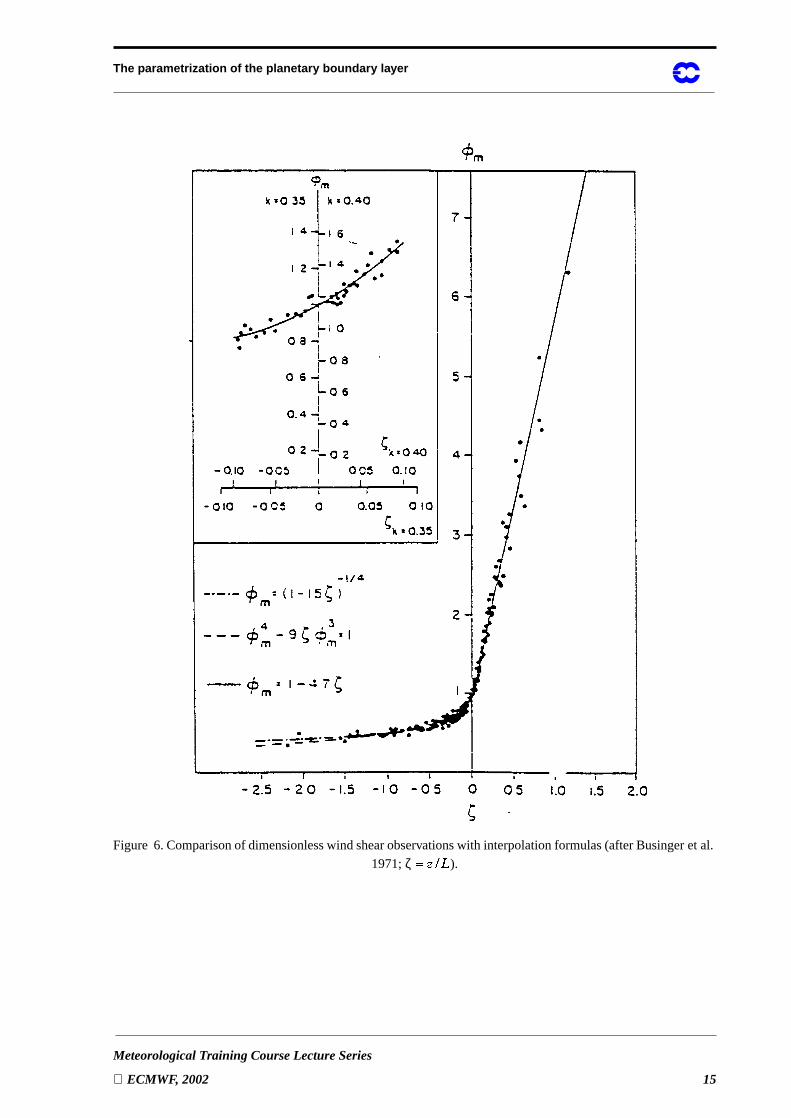
Thedimensionlessgradientfunctions(27)–(30)havebeenstudiedextensively with helpof field experimentsover
homogeneousterrain.Fig. 6 illustratesthis for φΜ with datafrom theKansasexperiment.Many empiricalforms
havebeenproposedfor thedimensionlessfunctions.Theexpressionsfor theunstablesurfacelayer(oftenreferred
to as the Dyer and Hicks profiles; seePaulson 1970,Dyer 1974 andHogstrom 1988 for a review) are:
(34)
(35)
(36)
(37)
and the linear relationship
(38)
asoriginally proposedby Webb(1970)is fairly consistentwith mostdatafor 0 6 �/. � 6 0.5(cf. Hogstrom,1988).
Analysisby Hicks (1976)of stablewind profilesabove theflat homogeneousterrainof the“Wangara”siteandby
Holtslag andDeBruin(1988)of Cabauwdataup to resultedin thefollowing expression(seealsoBel-
jaars and Holtslag, 1991)
(39)
(40)
where78( 1, 9:( 0.667,�;( 5 and<=( 0.35.Thisexpressionbehaveslike(38)for small�/. � valuesandapproaches
φM ~ 7 �1. � for large�1. � . The3/2 power in φH hasbeenintroducedto makeφH /φM proportionalto for
large values of�1. � (see discussion on stability functions in section3.3).
σθ
θ*------ f θ
��---- =
' M3 � � *------------ 1
φM-------=
' M
τ >d � d�⁄------------------
τ?d! d�⁄------------------= =
φM 1 16��----–
14---–
=
φH Q, 1 16��----–
12---–
for��---- 0<=
30.4=
φM φH Q, 1 5��---- for
��---- 0>+= =
� �⁄ 10≈
φM 1 7 ��---- 9 1 �@< ��----+ + < ��----–
exp+ +=
φH 1 123--- 7 ��----+
32---
9 1 � < ��----+ + < ��----–
exp+ +=
� �⁄( )1 2⁄
The parametrization of the planetary boundary layer
Meteorological Training Course Lecture Series
ECMWF, 2002 15
Figure 6.Comparisonof dimensionlesswind shearobservationswith interpolationformulas(afterBusingeretal.
1971;ζ ( �1. � ).
The parametrization of the planetary boundary layer
16 Meteorological Training Course Lecture Series
ECMWF, 2002
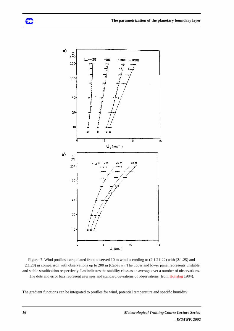
Figure 7. Wind profiles extrapolated from observed 10 m wind according to (2.1.21-22) with (2.1.25) and
(2.1.28) in comparison with observations up to 200 m (Cabauw). The upper and lower panel represents unstable
andstablestratificationrespectively. Lm indicatesthestabilityclassasanaverageoveranumberof observations.
The dots and error bars represent averages and standard deviations of observations (fromHoltslag 1984).
The gradient functions can be integrated to profiles for wind, potential temperature and specific humidity
The parametrization of the planetary boundary layer
Meteorological Training Course Lecture Series
ECMWF, 2002 17
(41)
(42)
(43)
(44)
with
(45)
(46)
where (47)
and
(48)
(49)
This canbederivedfrom thegradientfunctionswith helpof therelationshipφ = 1 – (η) dΨ . dη, whereη=�/. � .
Examplesof wind profilesaccordingto theempiricalformsof (45) and(48) areshown in Fig. 7 in comparison
with data.
It is clearthatthesefunctionsplayacrucialrole in parametrizationschemes.Thegradientfunctionsprovidedirect
expressionsfor exchangecoefficientsasthey relatefluxesto gradients.Theintegralprofile functionsaregenerally
usedin modelsthathave a modellevel in thesurfacelayerto specifytheprofilesbetweenthelowestmodellevel
andthesurface.Theexpressions(41) to (44)canin factbeseenasfinite differenceformsfor thelayerbetweenthe
surface and the lowest model level.
Limiting cases in surface layer similarity
In determininganalyticalformsfor thesimilarity functionsit is oftenusefulto considertheirasymptoticbehaviour.
Theneutrallimit (�/. � = 0) andthefreeconvectionlimit (A �/. � >>1)areof particularinterestbecausethey provide
information to limit the degrees of freedom in choosing analytical expressions.
In theneutrallimit with �/. � = 0, theObukhov lengthdropsoutasarelevantscaleandthereforethedimensionless
� τ >ρ3 � *
-------------�
� 0M---------
ΨM��----
–ln=
! τ?ρ3 � *
-------------�
� 0M---------
ΨM��----
–ln=
θ θs–� ′θ′–( )03 � *
----------------------�
� 0H--------
ΨM��----
–ln=
� � s–� ′ � ′–( )03 � *
----------------------�
� 0Q--------
ΨM��----
–ln=
ΨM 2 1 �+( ) 2⁄{ } 1 � 2+( ) 2⁄{ } �( ) π 2⁄+atan–ln+ln=
ΨH Q, 2 1 � 2+( ) 2⁄{ } for��---- 0<ln=
� 1 16��----–
14---
=
ΨM 7 ��----– 9 ��---- �<---–
< ��----– 9&�
<------–exp–=
ΨH 1 123--- 7 ��----+
32---
– 9 ��---- �<---–
< ��----– 9/�
<------– for��---- 0>exp–=
The parametrization of the planetary boundary layer
18 Meteorological Training Course Lecture Series
ECMWF, 2002
windgradienthastobeconstant.ThedimensionalwindgradientφM isbydefinitionequalto1becausetheempirical
constantis absorbedin thedefinitionandis calledtheVon Karmanconstant.Theexactvalueof theVon Karman
constanthasbeensubjectof considerabledebate.Valuesbetween0.35and0.42havebeenproposed,but 0.4is the
most widely accepted value now (e.g.Hogstrom, 1988).
Theotherlimiting casewith – �/. � >> 1 is calledthefreeconvectionlimit. A largevaluefor – �/. � implies that
theproductionof turbulenceby buoyancy is muchlarger thantheproductionby wind shearandthat the friction
velocity � * is irrelevantasscalingquantity. Theonly way to obtainindependenceof � * in thedimensionlesspo-
tentialtemperaturegradientexpressionis by choosinga1/3power law for – �/. � >> 1, as�
is proportionalto �by definition:
(50)
Alternatively a convective velocity scale can be defined based on the on the buoyancy flux
(51)
resulting in
(52)
The freeconvectionvelocity representsphysically thevelocity that largeeddies(e.g.thermals)typically have in
theconvective boundarylayer. It shouldbenotedthatequation(35) doesnot satisfytheconstraintasimposedby
thefreeconvectionlimit. In practicehowever (35) fits dataasaccuratelyasexpressionsthat tendto
for large –�/. � .
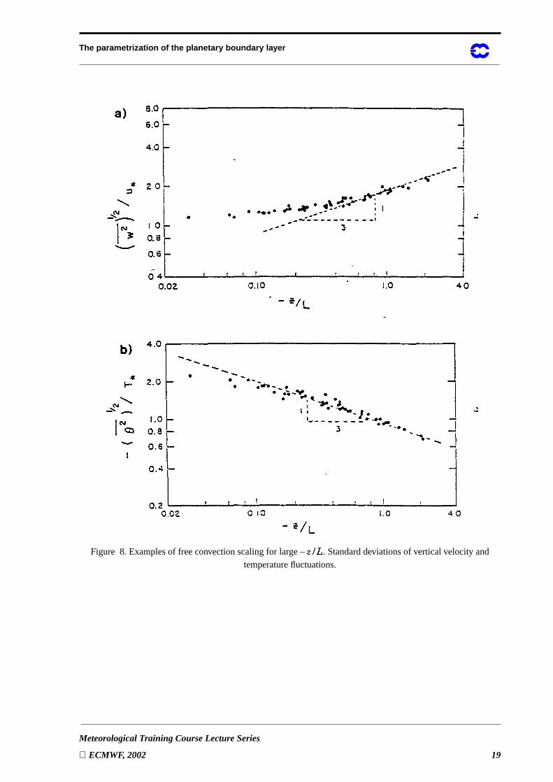
Anotherexampleof thefreeconvectionlimit is thescalingrelationfor thevariancesof velocity andtemperature
fluctuations (see alsoFig. 8):
(53)
(54)
With thedefinitionsof�
andθ* it canbeverifiedthat � * dropsoutof theserelations.Alternatively thesameforms
canbeexpressedin termsof thefreeconvectionvelocitywithoutusing � *. Theadvantageof theexpressionin z/L
is thatit providesa limiting form for large�/. � . Theseexamplesclearlyillustratethestrengthof similarity theory.
For theneutralandfreeconvectionlimit thesimilarity argumentsevenprovide theshapeof thefunctions,experi-
ments are only needed to determine the value of the constants (e.g. the Von Karman constant).
� *3
3 � � *
� ′θ′( )0
-------------------∂θ∂�------ φH
��---- ��----–
13---
∼=
� *s�θv----- � ′θ′v( )0�
13---
=
3 � � *s
� ′θ′( )0
-------------------∂θ∂�------ constant=
� �⁄–( ) 1– 3⁄
� ′2( )
12---
� *---------------- ��4 ��----–
13---
=
θ′2( )
12---
θ*-------------- � θ
��----–
13---–
=
The parametrization of the planetary boundary layer
Meteorological Training Course Lecture Series
ECMWF, 2002 19
Figure 8. Examples of free convection scaling for large –�/. � . Standard deviations of vertical velocity and
temperature fluctuations.
The parametrization of the planetary boundary layer
20 Meteorological Training Course Lecture Series
ECMWF, 2002
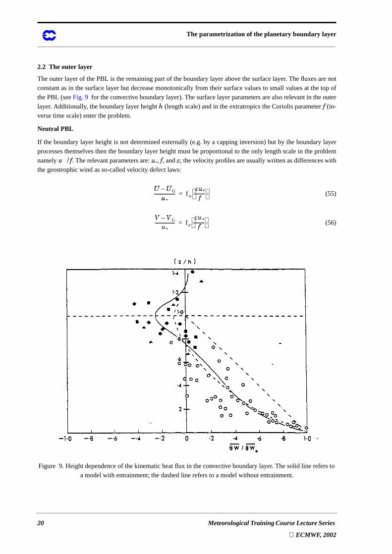
2.2 The outer layer
Theouterlayerof thePBL is theremainingpartof theboundarylayerabove thesurfacelayer. Thefluxesarenot
constantasin thesurfacelayerbut decreasemonotonicallyfrom their surfacevaluesto smallvaluesat thetop of
thePBL (seeFig. 9 for theconvectiveboundarylayer).Thesurfacelayerparametersarealsorelevantin theouter
layer. Additionally, theboundarylayerheight - (lengthscale)andin theextratropicstheCoriolis parameter� (in-
verse time scale) enter the problem.
Neutral PBL
If theboundarylayerheightis not determinedexternally (e.g.by a cappinginversion)but by theboundarylayer
processesthemselvesthentheboundarylayerheightmustbeproportionalto theonly lengthscalein theproblem
namely��B . � . Therelevantparametersare:� *, � , and� ; thevelocityprofilesareusuallywrittenasdifferenceswith
the geostrophic wind as so-called velocity defect laws:
(55)
(56)
Figure 9. Heightdependenceof thekinematicheatflux in theconvectiveboundarylayer. Thesolid line refersto
a model with entrainment; the dashed line refers to a model without entrainment.
� � G–
� *------------------- f 5 � � *
�--------- =
! ! G–
� *------------------ f C � � *
�--------- =
The parametrization of the planetary boundary layer
Meteorological Training Course Lecture Series
ECMWF, 2002 21
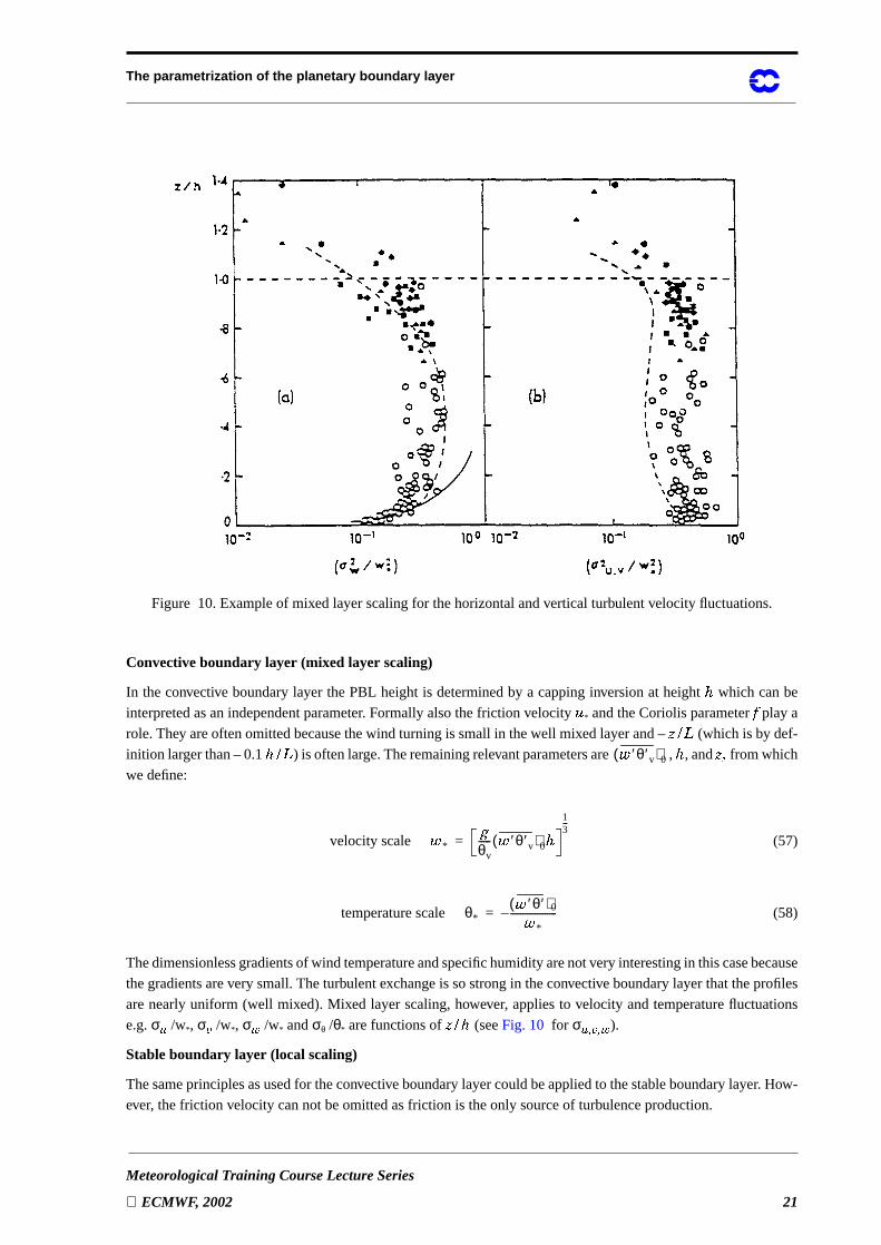
Figure 10. Example of mixed layer scaling for the horizontal and vertical turbulent velocity fluctuations.
Convective boundary layer (mixed layer scaling)
In theconvective boundarylayer thePBL heightis determinedby a cappinginversionat height - which canbe
interpretedasanindependentparameter. Formallyalsothefriction velocity � * andtheCoriolis parameter� playa
role.They areoftenomittedbecausethewind turningis smallin thewell mixedlayerand– �/. � (which is by def-
inition largerthan– 0.1 - . � ) is oftenlarge.Theremainingrelevantparametersare , - , and� � from which
we define:
(57)
(58)
Thedimensionlessgradientsof wind temperatureandspecifichumidityarenotveryinterestingin thiscasebecause
thegradientsareverysmall.Theturbulentexchangeis sostrongin theconvectiveboundarylayerthattheprofiles
arenearlyuniform (well mixed).Mixed layer scaling,however, appliesto velocity andtemperaturefluctuations
e.g.σ D /w*, σ E /w*, σ F /w* andσθ /θ* are functions of�/. - (seeFig. 10 for σ DHGIEJGKF ).
Stable boundary layer (local scaling)
Thesameprinciplesasusedfor theconvectiveboundarylayercouldbeappliedto thestableboundarylayer. How-
ever, the friction velocity can not be omitted as friction is the only source of turbulence production.
� ′θ′v( )0
velocity scale � *�θv----- � ′θ′v( )0 -
13---
=
temperature scale θ*� ′θ′( )0
� *-------------------–=
The parametrization of the planetary boundary layer
22 Meteorological Training Course Lecture Series
ECMWF, 2002
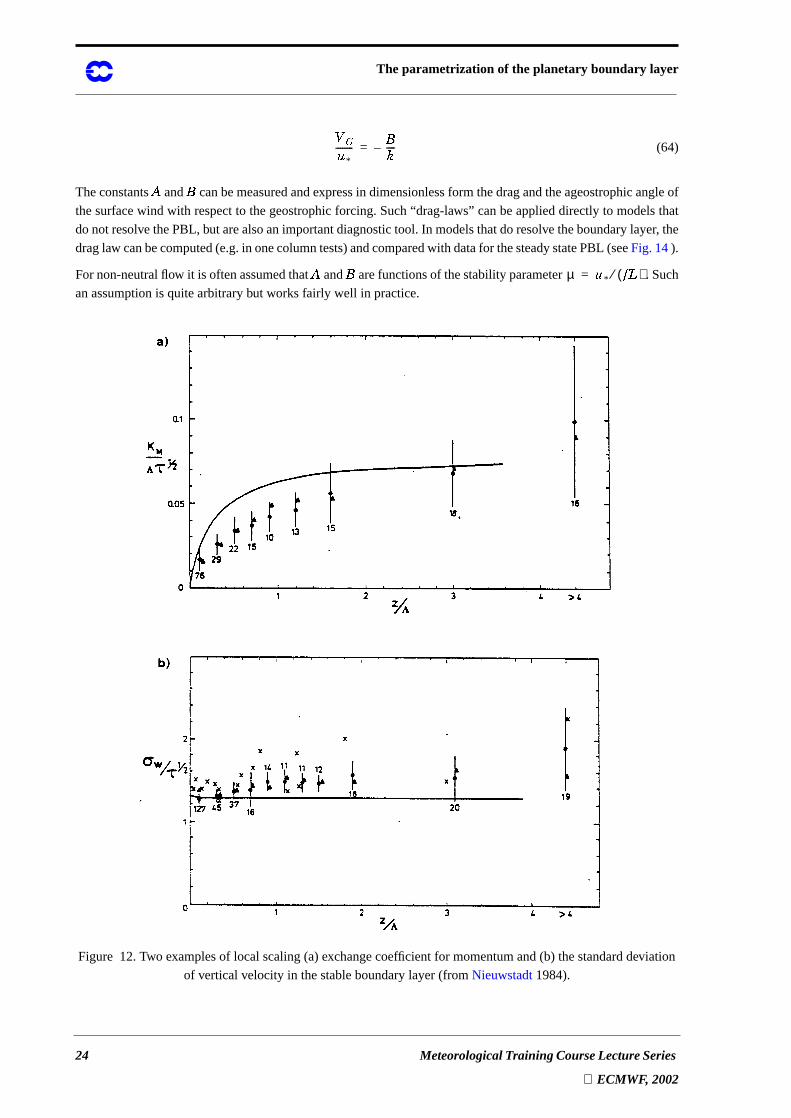
To limit thenumberof independentparametersNieuwstadt(1984)introducedtheideaof local scalingwhich can
bemadeplausiblein thefollowing way. In thestableboundarylayerturbulenceis generatedby shearproduction
anddestroyedby buoyancy andviscousdissipation.Sincebuoyancy is actingin theverticalcomponentit tendsto
limit theverticalextentoverwhichthemixing takesplaceandthereforelimits theturbulencelengthscale.Thede-
couplingof turbulencefrom thesurfacesuggestthat the local fluxesmight bemoresuitableasdirectscalingpa-
rameters.Thestrengthof this idealies in thefactthattheresultingfunctionsarenecessarilythesameastheones
for thesurfacelayersincethelocalfluxesareequalto thesurfacefluxeswhenthesurfaceis approached.Thismeans
thatexperimentaldatafrom thesurfacelayerandtheouterlayercanbecombined.For modelswith local closure
(asin theECMWFmodel)it alsomeansthattheclosureschemefor thesurfacelayerandtheouterlayercanbethe
same.
In theframework of local scalingtherelevantparametersare:the local fluxes and ,thebuoyancy pa-
rameter� /θv and height� . From these we define:
(59)
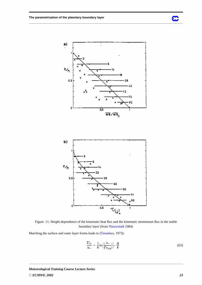
Localscalingimpliesthatdimensionlessquantitiesarefunctionsof �/. Λ insteadof �/. � . Examplesof localscaling
are given inFig. 12; the height dependence of momentum and heat fluxes is illustrated inFig. 11.
For large �/. Λ theturbulencelengthscaleis Λ andthepresenceof thesurfaceshouldhave no influence.This im-
plies that � shoulddropout of thescalingrelations.Theconsequencefor thedimensionlessgradientfunctionsis
thatthey becomelinearin �/. Λ for large�/. Λ becausethey have � asalengthscalein theirdefinition.Theprinciple
thatdimensionlessfunctionsbecomeindependentof � is called� -lessscaling.Theconsequencein Fig. 12 is that
the empirical functions tend to a constant for large�1. Λ.
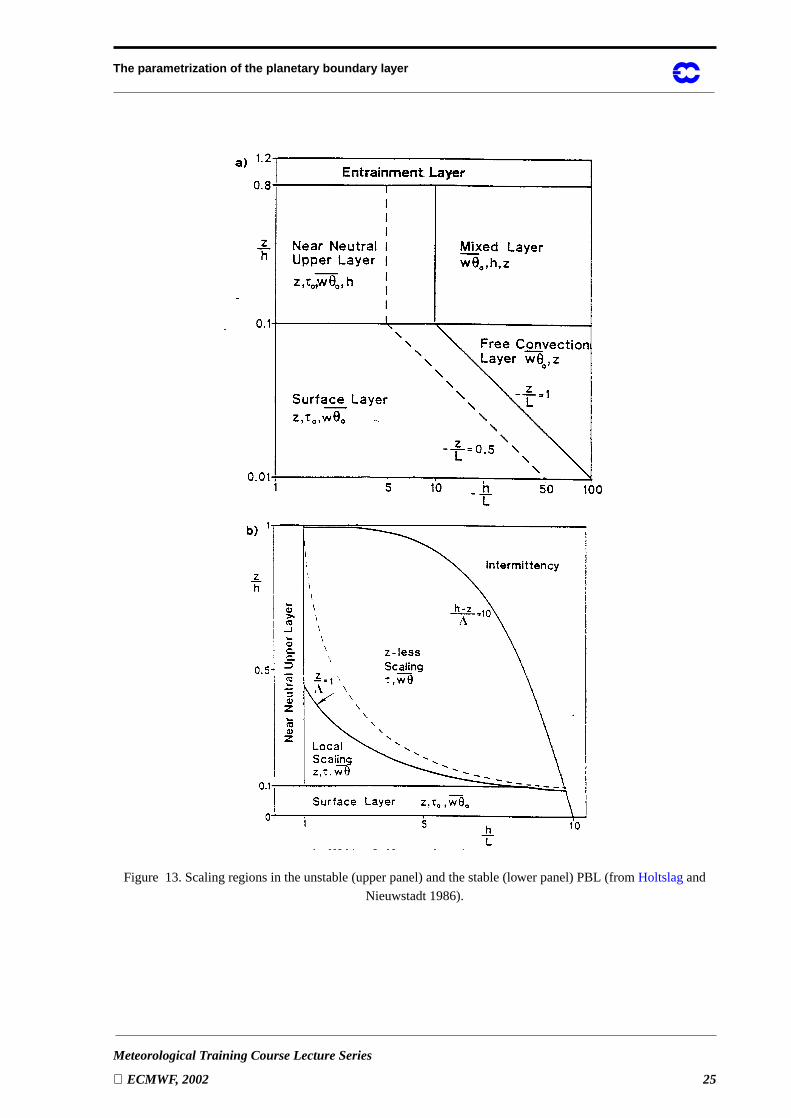
Thedifferentscalingregimesof theboundarylayeraresummarizedin Fig.13 for theunstableandstablePBL.The
dimensionlessheight�/. - andthedimensionlessstabilityparameter- . � areusedto delineatethedifferentscaling
regimes.
2.3 Matching of surface and outer layer (drag laws)
Theprofile functionsfor theneutralouterlayerwritten in velocity defectform mustbelogarithmicfor
andmustmatchthesurfacelayerprofiles.With thecoordinatesystemalignedwith thesurfacewind
and neutral stability:
surface layer limit for :
(60)
outer layer limit for :
(61)
(62)
τ ρ⁄ � ′θ′v
Λ τ ρ⁄ 3 2⁄–3 �
θv----- � ′θ′v
----------------------- (local Obukhov length) .=
� -⁄ 0→� ′ � ′( )0 0=
�L� 0M⁄ ∞→
�� *-----
13--- �� 0M---------
ln=
� -⁄ 0→
� � G–
� *-------------------
13--- � �� *------
const+ln=
! 0=
The parametrization of the planetary boundary layer
Meteorological Training Course Lecture Series
ECMWF, 2002 23
Figure 11. Height dependence of the kinematic heat flux and the kinematic momentum flux in the stable
boundary layer (fromNieuwstadt 1984)
Matching the surface and outer layer forms leads to (Tennekes, 1973):
(63)�NM� *--------
13--- � *
� � 0M------------
O 3----–ln=
The parametrization of the planetary boundary layer
24 Meteorological Training Course Lecture Series
ECMWF, 2002
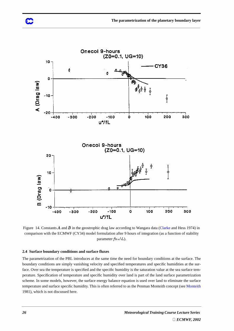
(64)
TheconstantsO andP canbemeasuredandexpressin dimensionlessform thedragandtheageostrophicangleof
thesurfacewind with respectto thegeostrophicforcing.Such“drag-laws” canbeapplieddirectly to modelsthat
donot resolvethePBL, but arealsoanimportantdiagnostictool. In modelsthatdoresolvetheboundarylayer, the
draglaw canbecomputed(e.g.in onecolumntests)andcomparedwith datafor thesteadystatePBL (seeFig.14).
For non-neutralflow it is oftenassumedthatO andP arefunctionsof thestabilityparameter . Such
an assumption is quite arbitrary but works fairly well in practice.
Figure 12.Two examplesof local scaling(a)exchangecoefficient for momentumand(b) thestandarddeviation
of vertical velocity in the stable boundary layer (fromNieuwstadt 1984).
! M� *--------
P 3----–=
µ � * � �( )⁄=
The parametrization of the planetary boundary layer
Meteorological Training Course Lecture Series
ECMWF, 2002 25
Figure 13. Scaling regions in the unstable (upper panel) and the stable (lower panel) PBL (fromHoltslag and
Nieuwstadt 1986).
The parametrization of the planetary boundary layer
26 Meteorological Training Course Lecture Series
ECMWF, 2002
Figure 14.ConstantsO andP in thegeostrophicdraglaw accordingto Wangaradata(ClarkeandHess1974)in
comparison with the ECMWF (CY34) model formulation after 9 hours of integration (as a function of stability
parameter� �RQ . � ).
2.4 Surface boundary conditions and surface fluxes
Theparametrizationof thePBL introducesat thesametime theneedfor boundaryconditionsat thesurface.The
boundaryconditionsaresimply vanishingvelocity andspecifiedtemperaturesandspecifichumiditiesat thesur-
face.Overseathetemperatureis specifiedandthespecifichumidity is thesaturationvalueat theseasurfacetem-
perature.Specificationof temperatureandspecifichumidity over land is partof the landsurfaceparametrization
scheme.In somemodels,however, thesurfaceenergy balanceequationis usedover landto eliminatethesurface
temperatureandsurfacespecifichumidity. This is oftenreferredto asthePenmanMonteithconcept(seeMonteith
1981), which is not discussed here.
The parametrization of the planetary boundary layer
Meteorological Training Course Lecture Series
ECMWF, 2002 27
Lookingmorecarefullyat theboundaryconditions,onerealizesthatanadditionalparametrizationproblemarises.
Theboundaryconditionsareconnectedto thesurfaceroughnesslengthswhichareextremelyimportantto thesur-
facefluxes.To illustratethis we assumethatwe have a modellevel nearthesurfacein theconstantflux layerat a
specifiedheight� 1 (in theECMWF model m). Thesurfacelayerprofilesareusedto specifytheboundary
condition:
(65)
(66)
(67)
(68)
Thelogarithmicprofilesarewritten in away that � , ! , θ and � have theirsurfacevaluesfor � = 0 (adisplacement
heightequalto the roughnesslengthhasbeenaddedto thevertical coordinate).The integrationconstantsin the
logarithmicprofilesarecalledroughnesslengthsbecausethey arerelatedto thesmallscalesurfaceinhomogenei-
tiesthatdeterminethesurfacedrag.In generaltheviscousforcesplaynoroleatall in thesurfacedrag(exceptover
averysmoothsea);thepressureforcesontheroughnesselementstransferthewind stressto thesurface(form drag)
anddosomoreefficiently thanviscousforcesbecausetheheightof roughnesselementstendsto belargerthanthe
thicknessof theviscouslayer. For heatandmoisturethesituationis slightly different.Formdraghasnoequivalent
for scalarquantities.The air-surfacetransferis throughan inter-facial sub-layerwheremoleculartransferdom-
nates. This implies that the roughness lengths for momentum, heat and moisture are generally different.
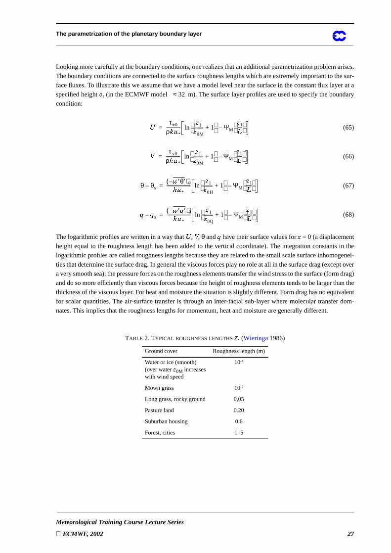
TABLE 2. TYPICAL ROUGHNESSLENGTHS S B (Wieringa1986)
Ground cover Roughness length (m)
Water or ice (smooth)(over waterT 0M increaseswith wind speed
10-4
Mown grass 10-2
Long grass, rocky ground 0,05
Pasture land 0.20
Suburban housing 0.6
Forest, cities 1–5
32≈
� τ > 0
ρ3 � *
-------------� 1
� 0M--------- 1+
ΨM
� 1�----- –ln=
! τ? 0
ρ3 � *
-------------� 1
� 0M--------- 1+
ΨM
� 1�----- –ln=
θ θs–� ′θ′–( )03 � *
----------------------� 1
� 0H-------- 1+
ΨM
� 1�----- –ln=
� � s–� ′ � ′–( )03 � *
----------------------� 1
� 0Q-------- 1+
ΨM
� 1�----- –ln=
The parametrization of the planetary boundary layer
28 Meteorological Training Course Lecture Series
ECMWF, 2002
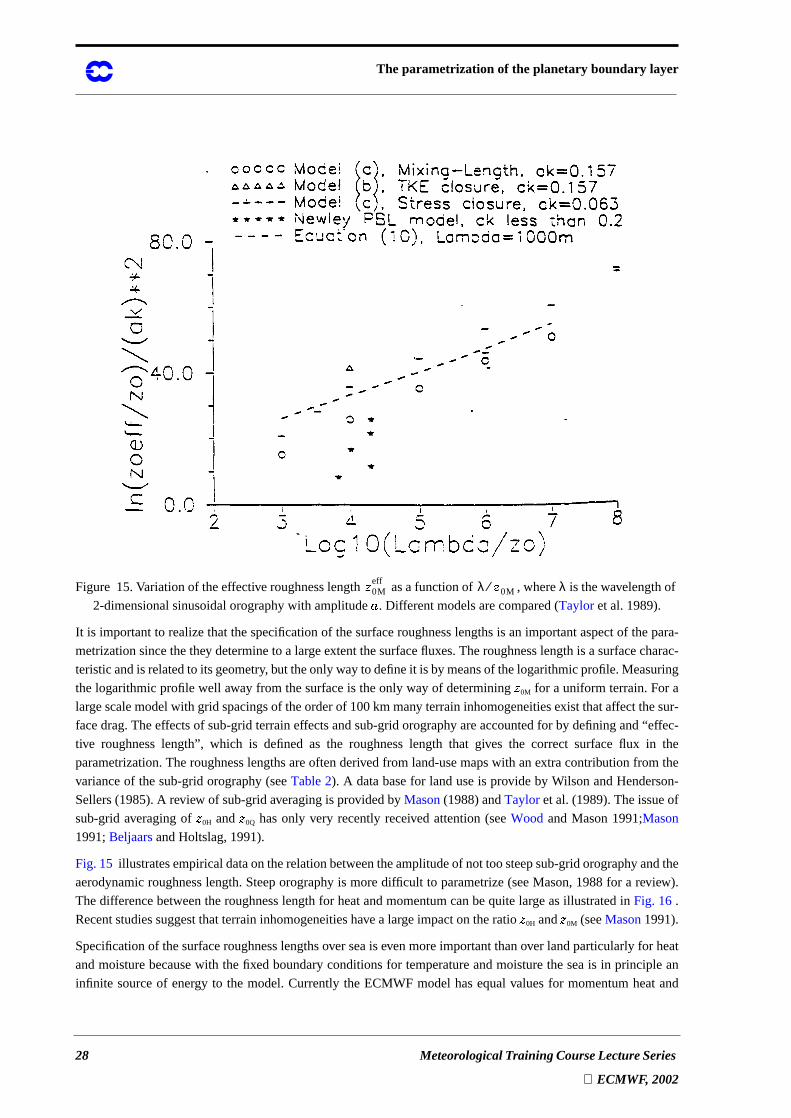
Figure 15.Variationof theeffectiveroughnesslength asafunctionof , whereλ is thewavelengthof
2-dimensional sinusoidal orography with amplitude7 . Different models are compared (Taylor et al. 1989).
It is importantto realizethatthespecificationof thesurfaceroughnesslengthsis animportantaspectof thepara-
metrizationsincethethey determineto a largeextentthesurfacefluxes.Theroughnesslengthis asurfacecharac-
teristicandis relatedto its geometry, but theonly wayto defineit is by meansof thelogarithmicprofile.Measuring
thelogarithmicprofile well away from thesurfaceis theonly way of determining� 0M for a uniform terrain.For a
largescalemodelwith grid spacingsof theorderof 100km many terraininhomogeneitiesexist thataffect thesur-
facedrag.Theeffectsof sub-gridterraineffectsandsub-gridorography areaccountedfor by definingand“effec-
tive roughnesslength”, which is definedas the roughnesslength that gives the correct surface flux in the
parametrization.Theroughnesslengthsareoftenderivedfrom land-usemapswith anextra contribution from the
varianceof thesub-gridorography (seeTable2). A databasefor landuseis provide by Wilson andHenderson-
Sellers(1985).A review of sub-gridaveragingis providedby Mason(1988)andTayloretal. (1989).Theissueof
sub-gridaveragingof � 0H and � 0Q hasonly very recentlyreceived attention(seeWood andMason1991;Mason
1991;Beljaars and Holtslag, 1991).
Fig.15 illustratesempiricaldataontherelationbetweentheamplitudeof nottoosteepsub-gridorography andthe
aerodynamicroughnesslength.Steeporography is moredifficult to parametrize(seeMason,1988for a review).
Thedifferencebetweentheroughnesslengthfor heatandmomentumcanbequitelargeasillustratedin Fig. 16 .
Recentstudiessuggestthatterraininhomogeneitieshavea largeimpacton theratio � 0H and� 0M (seeMason1991).
Specificationof thesurfaceroughnesslengthsoverseais evenmoreimportantthanover landparticularlyfor heat
andmoisturebecausewith thefixedboundaryconditionsfor temperatureandmoisturetheseais in principlean
infinite sourceof energy to the model.Currently the ECMWF modelhasequalvaluesfor momentumheatand
� 0Meff λ � 0M⁄
The parametrization of the planetary boundary layer
Meteorological Training Course Lecture Series
ECMWF, 2002 29
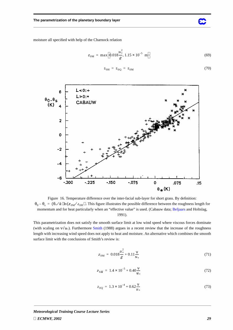
moisture all specified with help of the Charnock relation
(69)
(70)
Figure 16. Temperature difference over the inter-facial sub-layer for short grass. By definition:
. Thisfigureillustratesthepossibledifferencebetweentheroughnesslengthfor
momentum and for heat particularly when an “effective value” is used. (Cabauw data;Beljaars and Holtslag,
1991).
This parametrizationdoesnot satisfythesmoothsurfacelimit at low wind speedwhereviscousforcesdominate
(with scalingon ν . � B ). FurthermoreSmith (1988)arguesin a recentreview that the increaseof the roughness
lengthwith increasingwind speeddoesnotapplyto heatandmoisture.An alternativewhichcombinesthesmooth
surface limit with the conclusions of Smith’s review is:
(71)
(72)
(73)
� 0M max 0.018� *
2
�----- 1.15 10 5–× m, =
� 0H � 0Q � 0M= =
θ0 θs– θ*
3⁄( ) � 0M � 0H⁄( )ln=
� 0M 0.018� *
2
�----- 0.11ν� *-----+=
� 0 U 1.4 10 5–× 0.40ν� *-----+=
� 0Q 1.3 10 4–× 0.62ν� *-----+=
The parametrization of the planetary boundary layer
30 Meteorological Training Course Lecture Series
ECMWF, 2002
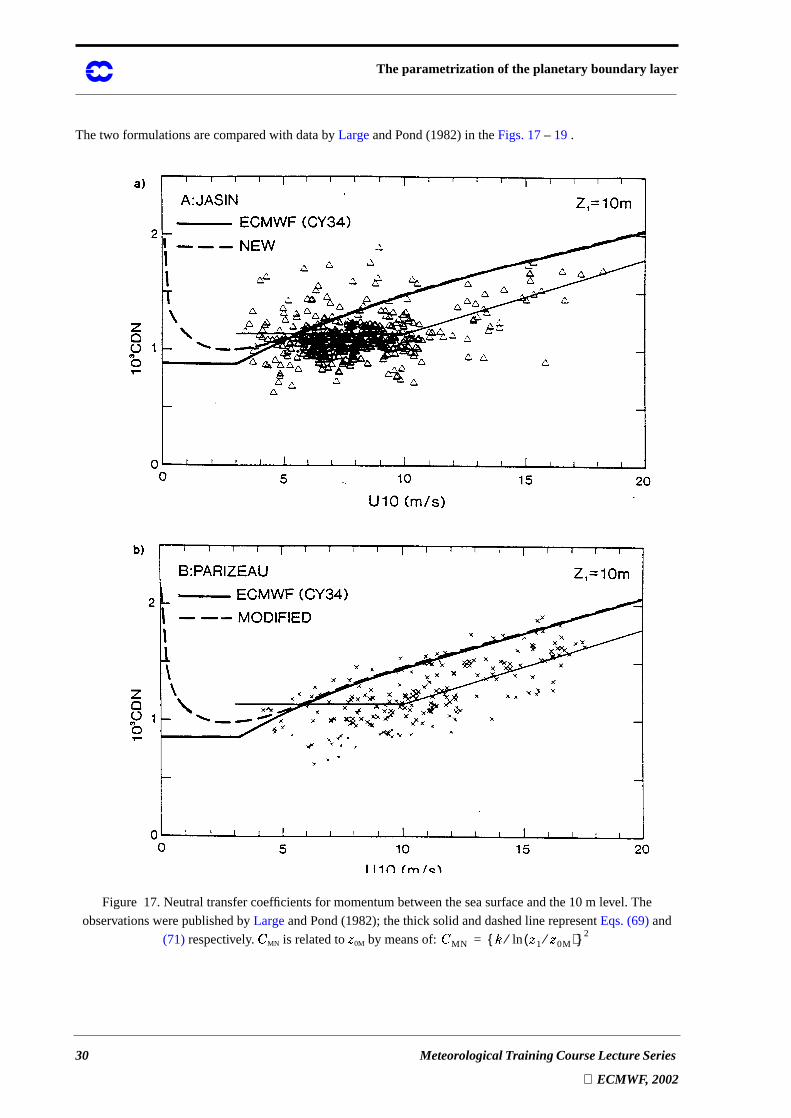
The two formulations are compared with data byLarge and Pond (1982) in theFigs. 17– 19 .
Figure 17. Neutral transfer coefficients for momentum between the sea surface and the 10 m level. The
observations were published byLarge and Pond (1982); the thick solid and dashed line representEqs. (69) and
(71) respectively. V MN is related to� 0M by means of:V MN
3 � 1 � 0M⁄( )ln⁄{ }2=
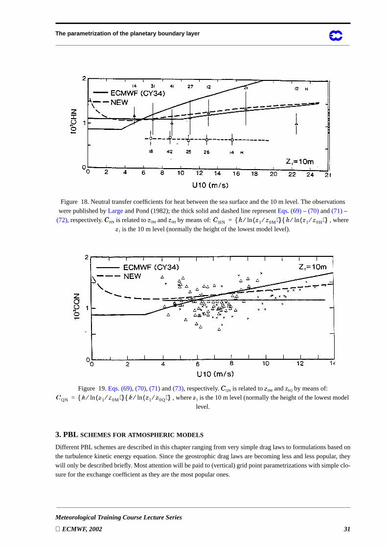
The parametrization of the planetary boundary layer
Meteorological Training Course Lecture Series
ECMWF, 2002 31
Figure 18. Neutral transfer coefficients for heat between the sea surface and the 10 m level. The observations
were published byLarge and Pond (1982); the thick solid and dashed line representEqs. (69) – (70) and(71) –
(72), respectively. V HN is relatedto � 0M and� 0H by meansof: , where� 1 is the 10 m level (normally the height of the lowest model level).
Figure 19.Eqs. (69), (70), (71) and(73), respectively. V QN is related to� 0M and z0Q by means of:
, where� 1 is the10m level (normallytheheightof thelowestmodel
level.
3. PBL SCHEMES FOR ATMOSPHERIC MODELS
DifferentPBL schemesaredescribedin thischapterrangingfrom verysimpledraglaws to formulationsbasedon
theturbulencekinetic energy equation.Sincethegeostrophicdraglaws arebecominglessandlesspopular, they
will only bedescribedbriefly. Mostattentionwill bepaidto (vertical)grid pointparametrizationswith simpleclo-
sure for the exchange coefficient as they are the most popular ones.
V HN
3 � 1 � 0M⁄( )ln⁄{ }3 � 1 � 0H⁄( )ln⁄{ }=
V QN
3 � 1 � 0M⁄( )ln⁄{ }3 � 1 � 0Q⁄( )ln⁄{ }=
The parametrization of the planetary boundary layer
32 Meteorological Training Course Lecture Series
ECMWF, 2002
3.1 Geostrophic transfer laws
Geostrophictransferlaws canbeusedto introducesomeeffectsof surfacefluxesin modelsthathave hardlyany
or no levelsin theboundarylayer. They arebasedonboundarylayersimilarity for thesteadystateboundarylayer.
A relationis assumedbetweenthemodelvariablesat the lowestmodellevel andthefluxesat thesurface,where
thelowestmodellevel is assumedto beat thetop of theboundarylayeror above theboundarylayer. Suchanap-
proachmakesonly sensein modelswith low resolutionnearthesurface.Thesimplestform of a bulk transferlaw
expressesthesurfacefluxesof momentum,heatandmoistureinto themodelvariables� G, ! G, θG, � G above the
boundary layer and surface valuesθs and� s in the following way:
(74)
(75)
(76)
(77)
The index G hasbeenusedhereto indicatevariablesabove theboundarylayer; for wind it canbe thoughtof as
geostrophicwind. Theconstants , and arechosenfrom field dataor adjustedon thebasisof model
performance.Differentvaluescanbechosenfor landandsea.Advantagesof thisschemeare:(i) theschemeis very
simpleand(ii) it is afirst orderapproximationfor theinfluenceof surfacefluxes.Disadvantagesare:(i) thescheme
doesnothaveadiurnalcycle,(ii) therearenoeffectsof stability, (iii) theempiricalcoefficientsareveryuncertain,
(iv) there are no forecast products in the PBL and (v) the physics of the PBL is poorly represented.
A second“bulk” scheme,which is very similar to thefirst one,introducesstability effectsin thetransfercoeffi-
cients , and in accordance with the similarity theory discussed inSection 2.3.
(78)
where , or , (79)
and , . (80)
TheconstantO dependsonstabilityandis thesameoneasin Eq.(63). ExperimentaldataonA is shown in Fig. 14
(ClarkeandHess1974).Thisformulationis slightly morerealisticthanthefirst onebut is verymuchlimited to the
simplesituations,for whichthetransferlawsareknown.However, with anappropriatelandsurfaceschemefor the
surfacetemperature and surfacemoisture , this schemeallows for diurnal variation of the surfacedrag
throughthe stability dependenceof parameterO . The morecomplicatedcaseof the unsteadyPBL, caseswith
strongadvection,baroclinicor inversioncappedPBL’sarenotexpectedto bewell capturedby bulk transferlaws.
� ′ � ′( )0 V M UG � G–=
� ′ � ′( )0 V M UG ! G–=
� ′θ′( )0 V H UG θG θs–( )–=
� ′ � ′( )0 V Q UG � G � s–( )–=
V M V H V Q
V M V H V Q
V M V H V Q13--- � *
� � 0M------------
O 3----–ln2–
= = =
O O � *
� �------ = O O -�----
=
� * � ′ � ′( )02 � ′ � ′( )0
2+{ }
12---
=� � *
3–3 �
θv-----
� ′θv′( )0
------------------------------------=
θs � s
The parametrization of the planetary boundary layer
Meteorological Training Course Lecture Series
ECMWF, 2002 33
3.2 Integral models (slab, bulk models)
In integral modelstheentireboundarylayer is characterizedby a limited numberof parameters(e.g.PBL depth,
meanvelocity, meantemperatureetc.).Prognosticequationsarederivedfor thesePBL characteristicsratherthan
for thebasicvariables.Themainadvantageis thatthePBL doesnothaveto beresolvedby theverticallayerstruc-
ture of the model.
Thebasicassumptionfor integralmodelsis thatasimilarity form existsfor themodelvariablese.g.for potential
temperature:
, (81)
where is a temperaturescaleand - theboundary-layerheight.Whentheform of f is known from field experi-
ments,Eq.(81)canbesubstitutedin theequationsof motionandintegratedfrom thesurfaceto � (W- . Theresulting
differential equations for and- describe the entire PBL without resolving it explicitly in the vertical.
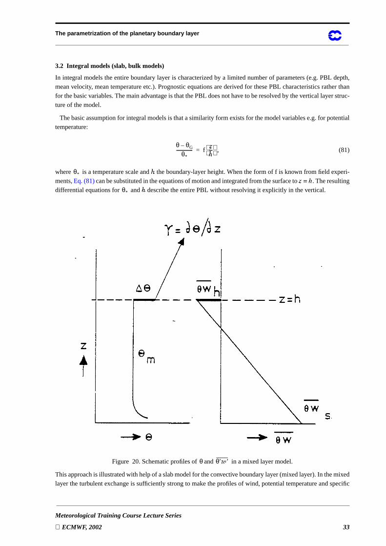
Figure 20. Schematic profiles ofand in a mixed layer model.
Thisapproachis illustratedwith helpof aslabmodelfor theconvectiveboundarylayer(mixedlayer).In themixed
layertheturbulentexchangeis sufficiently strongto make theprofilesof wind, potentialtemperatureandspecific
θ θG–
θ*--------------- f
�----
=
θ*
θ*
θ θ′ � ′
The parametrization of the planetary boundary layer
34 Meteorological Training Course Lecture Series
ECMWF, 2002
humidityapproximatelyuniformin thebulk of theboundarylayer(thesimplestpossibleexpressionfor f). Thenear
surfacepartshows gradients,but thesurfacelayer is relatively shallow anddoesthereforenot contributesignifi-
cantlyto thebudgetsof thetotalboundarylayer. Herewe limit to thebudgetof potentialtemperaturebecauseit is
themainquantitythatfeedsbackto thedynamicsof themixedlayer. Quantity representsthepotentialtemper-
aturein thebulk of themixedlayerandits timeevolution is determinedby heatfluxesat thesurfaceandthetopof
themixedlayer(Fig.20 illustratesthetemperaturestructureof thewell mixedlayer;seeDriedonksandTennekes,
(1984)):
, (82)
, (83)
, (84)
. (85)
In theseequations representsthepotentialtemperaturejumpat thetopof theboundarylayer, theentrain-
mentvelocity, thelargescaleresolvedverticalvelocityatheight- , andγ thestablelapserateabovethemixed
layer. Equations(82)–(85) describetheenergy budget,theheightandthetemperaturestepat thetop of themixed
layerandhaveasimplephysicalinterpretation.Therateof changeof theenergy of themixedlayeris proportional
to thedifferenceof heatflux at thesurfaceandthetop(Eq.(82)); theheightchangeof themixedlayerwith respect
to thelargescaleascentor descentis by definitiontheentrainmentvelocity (Eq.(83)); thetemperaturestepat � (- changesdueto temperaturechangesof the mixed layer andduea shift of the mixed layer with respectto the
stablelapserate(Eq.(84)); andtheentrainmentheatflux is theamountof air thatis entrainedtimesthetemperature
jump (Eq. (84)). This setof equationsis not closed;it hasto besupplementedby equationsfor thesurfacefluxes
andby anentrainmentassumption.Thesurfacefluxescanbeobtainedby usingsurfacelayerformulationsasdis-
cussed inSection 2.4. For the heat flux,Eq. (67) can be used with� somewhere in the mixed layer and .
To parametrize the entrainment we consider the equation for turbulent kinetic energy:
(86)
This equationdescribesthebalancebetweenshearproduction(I), buoyancy productionor destruction(II), trans-
portby turbulentvelocityandpressurefluctuations(III) anddissipation(IV). Theorderof magnitudeof thediffer-
ent terms typical for the entire mixed layer depth can be expressedin terms of velocity and length scales
characteristic for the mixed layer:
I:
II:
θm
- dθm
d�--------- � ′θ′( )0 � ′θ′( )0–=
d-d�------- � e � L+=
d∆θm
d�-------------- γ � e
dθm
d�---------–=
� ′θ′( )0 � e∆θ–=
∆θm � e
� L
θ θm=
∂$
∂ �------- = � ′ � ′∂ �∂�--------– � ′ � ′∂ !∂�-------–�ρ0----- � ′θv′+
I( ) I I( )
∂∂�------
$′ � ′ � ′ � ′
ρ------------+
+ ε .–
I I I( ) IV( )
� *3 -⁄� θv⁄( ) � ′θv′( )0 � *
3 -⁄+
The parametrization of the planetary boundary layer
Meteorological Training Course Lecture Series
ECMWF, 2002 35
III:
IV:
Theseestimateshavebeenmadeby assumingasinglelengthscale- asturbulencelengthscaleandfor theestima-
tion of thederivativesandby assumingthattheturbulentfluctuationshave magnitude (see(57) for its defini-
tion). It is importantto realizeherewhat themechanismof entrainmentis. Theenergy is producedby shearand
buoyancy in thebulk of themixedlayer. Most of theenergy is transferredto smallerandsmallerscalesandulti-
matelyconvertedinto heatby viscousdissipation.Someof it is diffusedupwardsby theturbulentmotionitself (e.g.
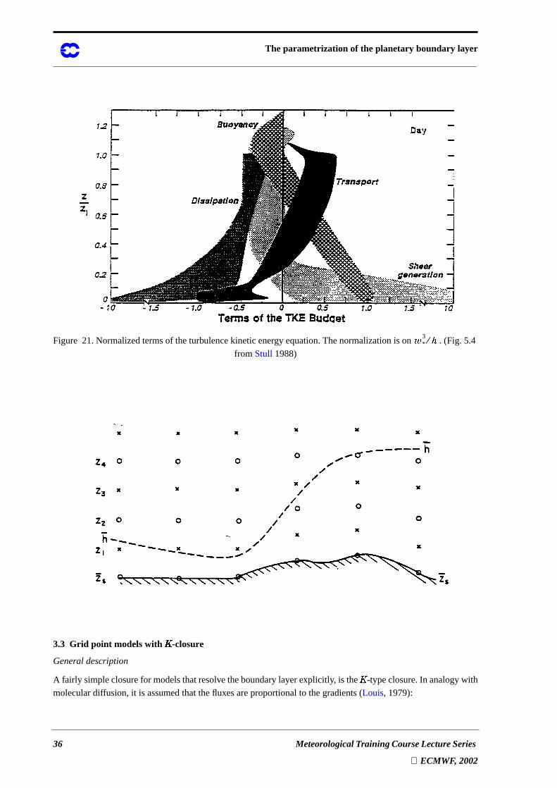
thermals)andpenetratesinto theinversionwhereit is destroyedby thenegative buoyancy (Fig. 21 illustratesthe
energy budgetof themixedlayer).Sotheentrainmentat thetop of themixedlayer is fed by upwarddiffusionof
turbulent kinetic energy produced in the bulk of the mixed layer.
Sincethedominanttermsareof theorderof , it is to beexpectedthat thebuoyancy flux at � (X- is also
proportional to this quantity. An obvious closure therefore is:
(87)
wherethe“entrainment”constant is determinedfrom experimentaldata.Thenumericalvalueof is about
0.2 (Driedonks and Tennekes 1984).
Theadvantagesof integralmodelsareobvious:(i) they arerelatively simple,(ii) they donot rely onverticalreso-
lution and(iii) they arephysically realisticfor simplecasesasthemixedlayer. Disadvantagesare:(i) this typeof
modelsis difficult to implementasthey involve a moving boundarycondition(thetop of theboundarylayer) for
theatmosphereabove thePBL, (ii) thesimilarity profilesarelessobvious for e.g.thestableboundarylayerand
virtually unknown for morecomplicatedboundarylayersase.g.thebaroclinicor cloudyboundarylayerand(iii)
thetransitionbetweendifferentscalingregimes(e.g.fromunstabletostable)aredifficult tohandle.Formixedlayer
modelsin particularit hasto beaddedthatthey performverywell for awell mixedquantityaspotentialtempera-
ture, but quite poorly for less well mixed quantities as momentum and specific humidity.
Becauseof thetechnicalcomplicationsof having a moving lower boundaryconditionin a forecastmodel,Dear-
dorff (1972)proposedto combinethe integral boundarylayerapproachwith a fixedverticalgrid structure.This
schemewasspeciallydesignedfor GCM’swith poorverticalresolution.Thediagnosedboundarylayerheightcan
bebelow andabovethelowestmodellevel (Fig.22). Theboundarylayerheightcanbeseenasanadditionalmodel
level at theheightwherethestructureof theatmospherechangesdrastically. After every time step,with thePBL
scheme the grid points inside the boundary layer are adjusted to the mixed-layer profile.
� *3 � *
3+( ) -⁄� *
3 � *3+( ) -⁄
� *
� *3 -⁄
� ′θv′( )0 V e � ′θv′( )0=
V e V e
The parametrization of the planetary boundary layer
36 Meteorological Training Course Lecture Series
ECMWF, 2002
Figure 21.Normalizedtermsof theturbulencekineticenergy equation.Thenormalizationis on . (Fig. 5.4
from Stull 1988)
Figure 22. Grid point structure inDeardorff’s (1972) PBL model.
3.3 Grid point models with Y -closure
General description
A fairly simpleclosurefor modelsthatresolvetheboundarylayerexplicitly, is the' -typeclosure.In analogywith
molecular diffusion, it is assumed that the fluxes are proportional to the gradients (Louis, 1979):
� *3 -⁄
The parametrization of the planetary boundary layer
Meteorological Training Course Lecture Series
ECMWF, 2002 37
, (88)
. (89)
Theexchangecoefficient ' is notapropertyof thefluid asin moleculardiffusion,but dependsontheflow. Surface
layer similarity provides the formulation for' near the surface (i.e. in the lowest model layer):
, (90)
whereZ[( 3 � . Useof thesameexpressionin theouterlayer (above the lowestmodellevel), would beconsistent
with theideasof local scaling(Section2.2) for thestableboundarylayer, providedthat , and arepro-
portionalto � for large �/. � . In this way thelengthscale� dropsout for large � . Two problemsarisefrom sucha
simpleextensionof surfacelayersimilarity bothrelatedto thelackof anupperboundto Z : (i) thediffusioncoeffi-
cientbecomesverylargein neutralsituationsand(ii) with differentfrom in stablesituations(necessaryfor
reasonsto beexplainedlater),localscalingbreaksdown and Z remainsanessentialpartof theparametrization.To
limit the length scaleBlackadar (1962) proposed the following expression:
(91)
This formulationobeys surfacelayersimilarity andis consistentwith local scalingfor thestableboundarylayer.
Theonly additionalparameterthathasbeenintroducedis theasymptoticlengthscaleλ, which is oftenthesame
for momentumandheat.The ideais that the turbulencelengthscaleis limited by the boundarylayer height.In
someparametrizationsλ ~ �RQ . � or λ ~ - , where- is adiagnosedboundarylayerheight.Sincetheresultsarenot
very sensitive to the exact value ofZ , this parameter is often chosen constant.
Expressions(90) containφ which dependson �/. � in thesurfacelayerandthereforeon thesurfacefluxes.Above
thesurfacelayer theφ-functionsdependon Z . 3 � insteadof �/. � to beconsistentwith the ideasof local scaling.
An inconvenientaspectof Eq. (90) is that it containsfluxeswhich makestheclosurean implicit one.To find an
explicit closure we substitute the closure assumptions in the definition of the Obukhov length and obtain:
(92)
This is a relationbetweenthegradientRichardsonnumberand Z . � which canbesolvednumericallywhentheφ-
functionsarespecified.Insteadof closureassumption(90) it is muchmoreefficient to specifystability functions
that depend on the Richardson number because then we have the fluxes explicitly in terms of model variables:
(93)
where and , and by definition: .
� ′ � ′ ' M∂ �∂�-------- ,–= � ′ � ′ ' M
∂ !∂�-------–=
� ′θ′ ' H∂θ∂�------ ,–= � ′ � ′ ' H
∂ �∂�------=
' MZ 2
φM2
------- dUd�------- , ' M
Z 2
φMφH------------- dU
d�-------= =
φM φH φQ
φM φH
1Z---
13 �------ 1λ---+=
� * �θv-----
dθv
d�--------
dUd�-------
2------------- Z3 �-------
φH
φM2
-------= =
' M Z 2\M
dUd�------- , ' H Z 2\
HdUd�------- ,==
\M
\M
� *( )= \H
\H
� *( )= \M φM
2– , \H φMφH( ) 1–= =
The parametrization of the planetary boundary layer
38 Meteorological Training Course Lecture Series
ECMWF, 2002
Equation(93) is theclosureasit is actuallyusedin many models.Thefunctions and arespecifiedasan-
alytical functionsof� * or aretabulated.In bothcasesthey arederivedfrom empiricaldataon and which
arefunctionsof �/. � (or Z . 3 � ), sotheindependentvariablehasbeentransformedfrom �/. � (or Z . 3 � ) to� * with
Eq. (92).
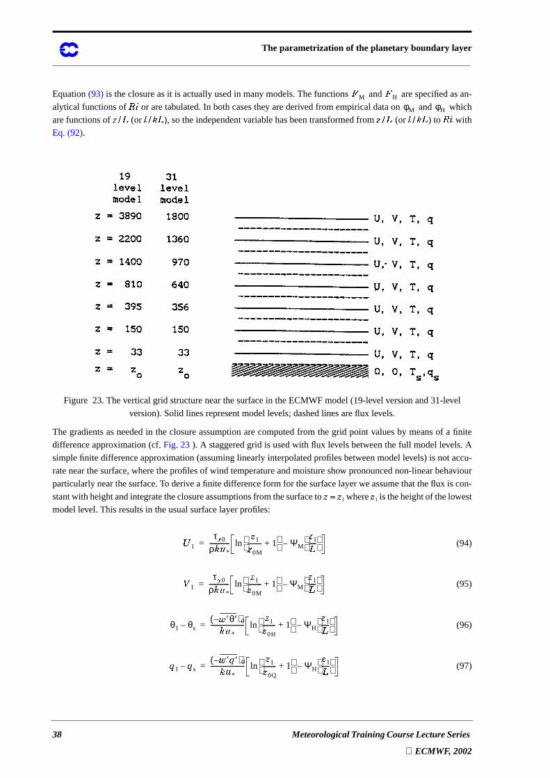
Figure 23. The vertical grid structure near the surface in the ECMWF model (19-level version and 31-level
version). Solid lines represent model levels; dashed lines are flux levels.
Thegradientsasneededin theclosureassumptionarecomputedfrom thegrid point valuesby meansof a finite
differenceapproximation(cf. Fig. 23 ). A staggeredgrid is usedwith flux levelsbetweenthefull modellevels.A
simplefinite differenceapproximation(assuminglinearly interpolatedprofilesbetweenmodellevels)is notaccu-
ratenearthesurface,wheretheprofilesof wind temperatureandmoistureshow pronouncednon-linearbehaviour
particularlynearthesurface.To deriveafinite differenceform for thesurfacelayerweassumethattheflux is con-
stantwith heightandintegratetheclosureassumptionsfrom thesurfaceto � ( � 1 where� 1 is theheightof thelowest
model level. This results in the usual surface layer profiles:
(94)
(95)
(96)
(97)
\M
\H
φM φH
� 1
τ > 0
ρ3 � *
-------------� 1
� 0M--------- 1+
ΨM
� 1�----- –ln=
! 1
τ? 0
ρ3 � *
-------------� 1
� 0M--------- 1+
ΨM
� 1�----- –ln=
θ1 θs–� ′θ′–( )03 � *
----------------------� 1
� 0H-------- 1+
ΨH
� 1�----- –ln=
� 1 � s–� ′ � ′–( )03 � *
----------------------� 1
� 0Q-------- 1+
ΨH
� 1�----- –ln=
The parametrization of the planetary boundary layer
Meteorological Training Course Lecture Series
ECMWF, 2002 39
Theseexpressionscanbeinterpretedasanexactfinite differencerepresentationof thelowestmodellayer. Unfor-
tunatelyit is animplicit formulationasit contains . Again we canrelatethe“flux-stability parameter”
to the bulk Richardson number :
(98)
(99)
Thisequationrelates� * b to � 1 /
�, � 1/� 0H and� 1/� 0M. For computationalefficiency thestability functionsareusually
representedin termsof thebulk Richardsonnumber� * b. Thesurfacefluxesof momentum( and ), heat(]W^
and water vapour_a`�b are expressed in model variables at the lowest model level in the following way:
(100)
(101)
(102)
(103)
where
(104)
(105)
(106)
With the neutral transfer coefficients defined as:
(107)
� �⁄ � �
⁄� * b
� * b�θv-----
� 1 θv1 θv0–( )
U12
--------------------------------=
� 1�-----� 1
� 0H-------- 1+
ΨH
� 1�----- –ln
� 1
� 0M--------- 1+
ΨM
� 1�----- –ln
2----------------------------------------------------------------=
τ > τ?
τ >ρ----- V M U1 � 1=
τ?ρ----- V M U1 ! 1=
]ρ �� ---------– V H U1 θ1 θs–( )=
`ρ----– V Q U1 � 1 � s–( )=
V M V MN\
M
� * b
� 1
� 0M---------
� 1
� 0H--------, ,
=
V H V QN\
Q� * b
� 1
� 0M---------
� 1
� 0H--------, ,
=
V Q V MN\
M
� * b
� 1
� 0M---------
� 1
� 0H--------, ,
=
V MN
3� 1
� 0M---------
ln
--------------------
2
=
The parametrization of the planetary boundary layer
40 Meteorological Training Course Lecture Series
ECMWF, 2002
(108)
(109)
The closureassumptionsarehiddennow in the empirical functionsof the Richardsonnumber, which arenever
measureddirectly. The reasonis that they dependon the surfaceconditions(surfaceroughnesslengths)which
makesit difficult to determinethemdirectlyfrom data.Experiments,however, doprovidedataonthe or func-
tions.Fromtherewe canderive numericallythe \ functionsfor differentsurfaceroughnesslengthsandmake an
empiricalfit to beusedin theforecastmodel.However the\ functions(104)–(106)dependon threedifferentpa-
rametersandit canbedifficult to obtainsimpleempiricalexpressionsthatareaccuratefor all possiblevalesof the
parameters.In many modelsthe threeroughnesslengthsarethesamewhich reducesthenumberof independent
parameters to 2, but the empirical functions can still be fairly inaccurate as will illustrated subsequently.
The stability functions
Themaindifficulty with ' -closureis thespecificationof thestability functions.Louis et al. (1982)give anover-
view of how thesefunctionhaveevolvedin theoperationalECMWFmodelastheresultof adjustmentsonthebasis
physicalargumentsandmodelperformance.ThefunctionsthathavebeenusedsinceDecember1981are(Louiset
al. 1982):
(110)
(111)
(112)
(113)
where9W( 5, �c( 5, and<2( 5, and
V HN
3� 1
� 0H--------
ln
--------------------
2
=
V QN
3� 1
� 0Q--------
ln
--------------------
2
=
φ Ψ
\M 1
29 � * 0
1 V 0 � * 0–( )1 2⁄+----------------------------------------- for
� * 0 0<–=
\H 1
39 � * 0
1 V 0 � * 0–( )1 2⁄+----------------------------------------- for
� * 0 0<–=
\M
1
1 29 � * 0 1 < � * 0+( ) 1 2⁄–+-------------------------------------------------------------- for
� * 0 0>=
\H
1
1 39 � * 0 1 < � * 0+( )1 2⁄+------------------------------------------------------------ for
� * 0 0>=
V 0 39/�3 2 1
� 1
� 0M---------+
1 2⁄
1� 1
� 0M---------+
ln2
------------------------------------- in the surface layer, and=
V 0 Z 2
3� 2-------- above the surface layer.=
The parametrization of the planetary boundary layer
Meteorological Training Course Lecture Series
ECMWF, 2002 41
Extensivediagnosticsof operationalforecastshasshown thatthediffusionwastoostrongin themiddleandupper
troposphere,wherethejet streamwaspartially smearedout by theactionof theverticaldiffusionscheme.It was
thereforedecidedto make a roughestimateof theboundarylayerheightandto switchoff theschemeabove the
boundarylayerin stablesituations.Thischangewasintroducedoperationallyin January1988.Thepoorperform-
anceof theschemeabovetheboundarylayercanbeattributedto theshapeof thestability functionin theRichard-
son number range of 0.1 to 1.
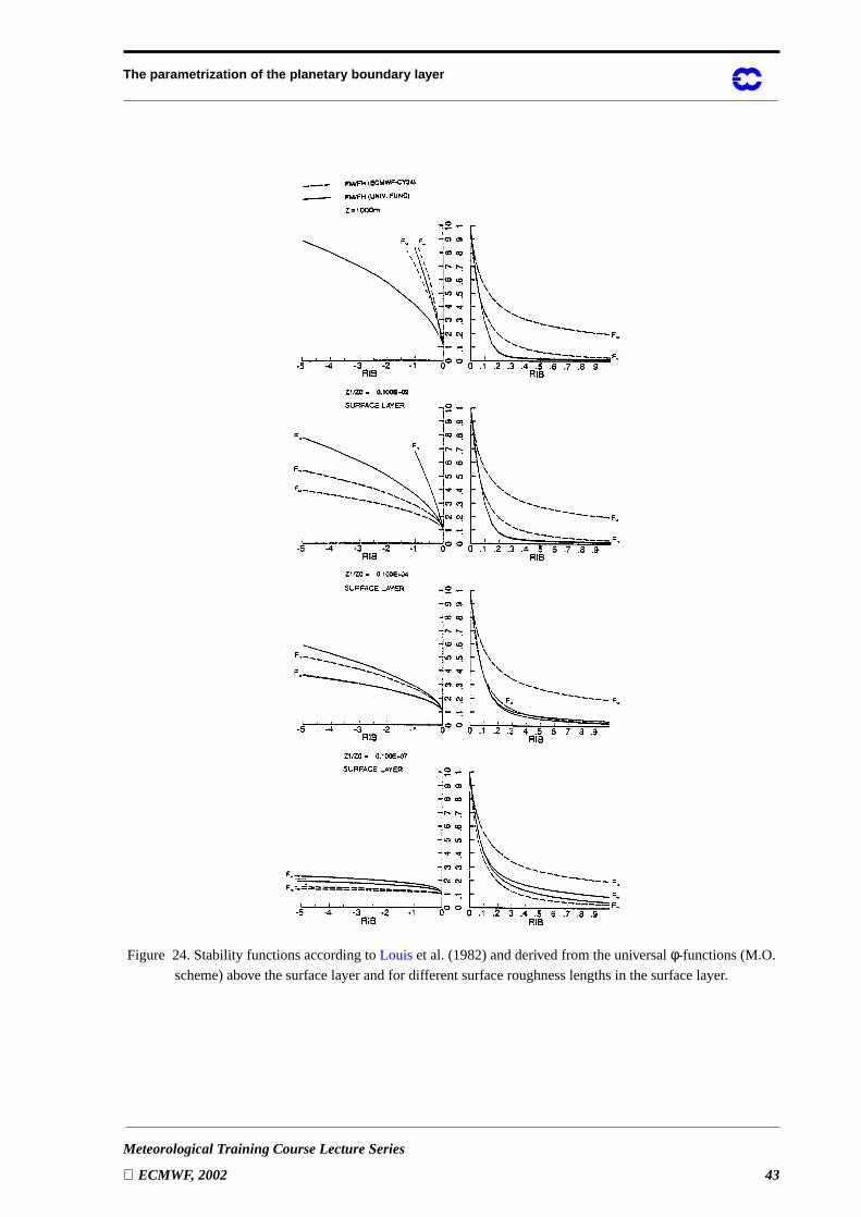
An alternative form of thestability functions(the\ _ � *d^ functions)canbederivedfrom theφ functions(34)–(35)
in unstablesituationsand(39)–(40) in stableflow. We will call themtheM.O. functions.Thecomparisonof the
stability functionsis shown in Fig. 24 . We seethat for positive Richardsonnumbersthe functionsderived from
and dependon thesurfaceroughnesslength.Themostpronounceddifferenceabove thesurfacelayer is
thattheM.O. functionsgivemuchsmallervaluesabove� * = 0.1in comparisonto theLouisetal. (1982)functions.
It shouldberealizedthattheshapeof thestability functionsis subjectto anongoingdebate(Hogstrom1988).The
difficultiesoriginatefrom limitations in theconceptof local diffusionandfrom uncertaintiesin theexperimental
data.An exampleof thefirst difficulty is theunstableor convectiveboundarylayerwherethediffusionis not local.
Thereasonthatalocalschemestill performsreasonablywell is thatthecoefficientsbecomelargeandthereforethe
profilesvirtually uniform irrespective of theexactmagnitudeof thediffusioncoefficients.For quantitiesthatare
not well mixed in theconvective boundarylayerase.g.moistureor wind in a baroclinicPBL, a local schemeis
expectedto belessappropriate.A secondexampleof thesameproblemis diffusionin stablystratifiedflow in the
intermittentregime.Localscalingworksfairly well in thefully turbulentregimeupto Richardsonnumbersof 0.2.
Beyond0.2,turbulencebecomesintermittentandthediffusivecharacteristicsarenotwell understood.Also wave-
turbulenceinteractionis a relevantprocessin this range.The reportedmagnitudeof thediffusioncoefficientsin
clear-air turbulence(Richardsonnumbersbetween0.2and1) variesby andorderof magnitudefrom onestudyto
the other(KennedyandShapiro1980;Uedaet al. 1981;Kondo et al. 1978;Nieuwstadt1984;Kim andMahrt
1991).Theshapeof functions and asexpressedby Eqs.(39)–(40) is reasonablywell documented(seeBel-
jaarsandHoltslag1991)for weakandmoderatestability. Theratio , however, is inspiredby theideathat
this ratio shouldbecomeproportional� * for largeRichardsonnumbers(seeEq. (92)). This particularasymptotic
behaviour is muchlessdocumented,but is quit relevantto thetransformationfrom �/. � to� * in Eq.(92). Another
parameterthatdeterminesto alargeextentthediffusionin theclear-air turbulencedomainis theasymptoticlength
scaleλ. A simpleparametrizationstrategy is to selectstability functionswhich arereasonablywell documented
from� * = 0 to
� * = 0.2,applyphysicalconstraintsfor largeRichardsonnumbersasin Eqs.(39)–(40) andadjust
λ to obtainreasonablediffusioncoefficientsin theclearair turbulencedomaine.g.onthebasisof databy Kennedy
and Shapiro (1980).
One column simulations
To illustratethecharacteristicsof ' -closure,asinglecolumnversionof theverticaldiffusionschemehasbeenin-
tegratedover9 hourswith constantgeostrophicforcingandconstantforcingfrom thesurface.In thisway, anearly
steadystateis obtained.Theselectedforcing is aconstantgeostrophicwind of 10 m/sanda constantsurfaceheat
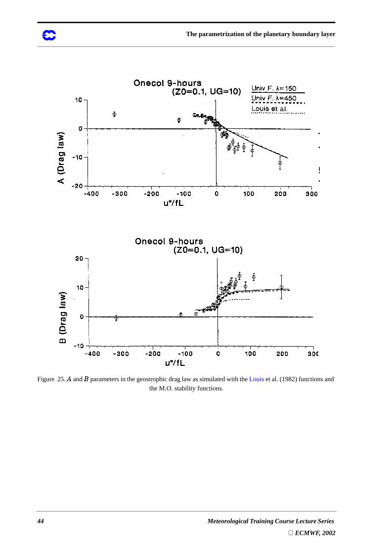
flux. Thesurfaceroughnesslengthis 0.1m. Fig. 25 shows theO andP parametersin thedraglaw of Eqs.(63) –
(64)astheresultof theparametrizationwith Louisetal. (1982)stabilityfunctionsandwith theM.O. stabilityfunc-
tions.Thecomparisonwith empiricaldatashowslittle difference;themaindifferenceis thattheM.O schemecov-
ersa muchlargerdimensionlessstability rangethantheLouis et al. schemefor thesamerangeof surfacefluxes.
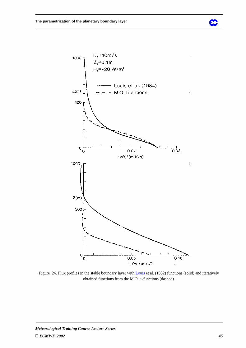
Thedifferencebetweenthetwo schemesis moreobviousin theFigs.26 and27 for a downwardheatflux of 20
W/m.Firstof all weseathatthesurfacestressis muchsmallerwith theM.O. schemeandthatthePBL is lessdeep.
Boundarylayerheightswith theM.O. schemearemuchmorerealisticandcomparemuchbetterwith dataasfor
instanceexpressedby theempiricalequilibriumheightsproposedby Zilitink evich (1972)or observationsby Nieu-
wstadt (1981).
φM φH
φM φH
φM φH⁄
The parametrization of the planetary boundary layer
42 Meteorological Training Course Lecture Series
ECMWF, 2002
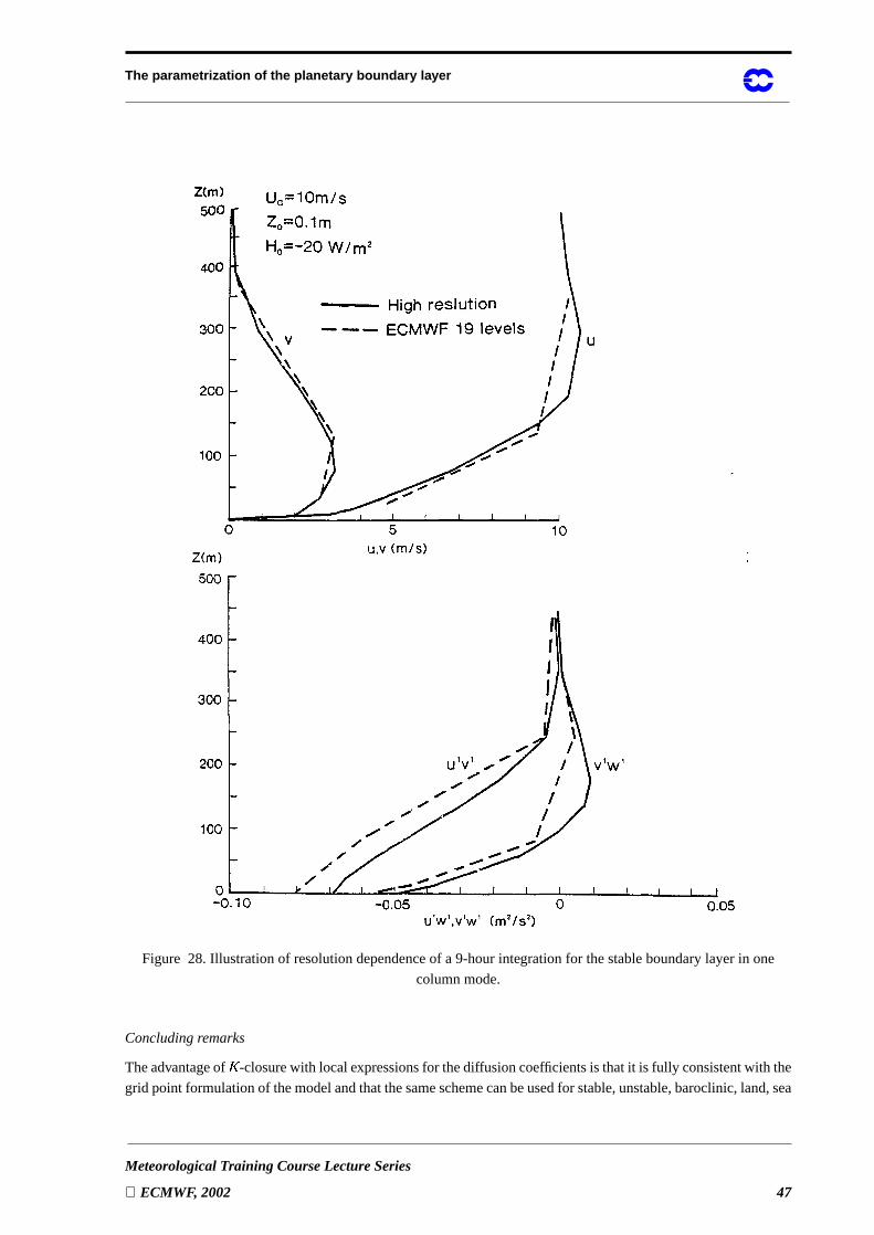
With arelatively low numberof grid pointsin thePBL, significantdiscretizationerrorscanbeexpected.Theshal-
low stableboundarylayercouldbeparticularlyaffectedasit is only resolvedby two or threemodellevels.The
effect of resolutionon thestructureof thestableboundarylayeris shown in Fig. 28 , wherea simulationwith the
19-level modelresolutionis comparedto a simulationwith threetimesasmany levels.We seethattheresultsare
very similar andthatthelow resolutionsimulationis fairly accurate.Theunexpectedrobustnessof thenumerical
schemeis relatedto thetreatmentof thesurfacelayerwhereaconsiderablepartof theshearandtemperaturegra-
dientsareconcentrated.In thesurfacelayertheschemeusestheintegral profile functions(94)–(97) asa bulk for-
mulationratherthanafinite differenceform. It is known from otherapplicationsthattheintegralprofile functions
are quite accurate also when extrapolated outside the surface layer (VanWijk et al. 1990).
The parametrization of the planetary boundary layer
Meteorological Training Course Lecture Series
ECMWF, 2002 43
Figure 24. Stability functions according toLouis et al. (1982) and derived from the universalφ-functions (M.O.
scheme) above the surface layer and for different surface roughness lengths in the surface layer.
The parametrization of the planetary boundary layer
44 Meteorological Training Course Lecture Series
ECMWF, 2002
Figure 25.O andP parametersin thegeostrophicdraglaw assimulatedwith theLouisetal. (1982)functionsand
the M.O. stability functions.
The parametrization of the planetary boundary layer
Meteorological Training Course Lecture Series
ECMWF, 2002 45
Figure 26. Flux profiles in the stable boundary layer withLouis et al. (1982) functions (solid) and iteratively
obtained functions from the M.O.φ-functions (dashed).
The parametrization of the planetary boundary layer
46 Meteorological Training Course Lecture Series
ECMWF, 2002
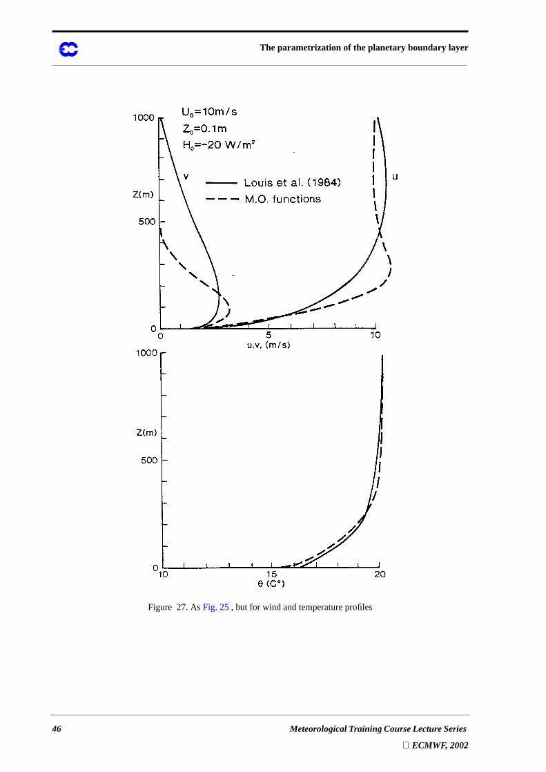
Figure 27. AsFig. 25, but for wind and temperature profiles
The parametrization of the planetary boundary layer
Meteorological Training Course Lecture Series
ECMWF, 2002 47
Figure 28. Illustration of resolution dependence of a 9-hour integration for the stable boundary layer in one
column mode.
Concluding remarks
Theadvantageof ' -closurewith localexpressionsfor thediffusioncoefficientsis thatit is fully consistentwith the
grid point formulationof themodelandthatthesameschemecanbeusedfor stable,unstable,baroclinic,land,sea
The parametrization of the planetary boundary layer
48 Meteorological Training Course Lecture Series
ECMWF, 2002
etc.A disadvantageis thata numberof modellevelsareneededto resolve theboundarylayer. On theotherhand,
it is quite remarkablethat theschemeperformsfairly well with 2 levels in a shallow stableboundarylayer. The
reasonis thatthesurfacelayerapproximationis exactin thesensethatthesurfacelayerprofilebetweenthesurface
andthelowestmodellevel is representedexactly. Theresolutionis only neededto obtainareasonableshearstress
profile,but flux profilesaregenerallyfairly linearasfunctionof heightandcanberepresentedwith a few points
only. Properresolutionis neededhoweverto resolveinversions.Sincethepositionof theinversionis variable,good
resolutionis neededtroughout thelower troposphere(Beljaars1991).This is obviouslyadisadvantagecompared
to mixedlayermodelswherea dedicatedmodelvariableexiststo keeptrackof theinversionheight.Anotherdis-
advantageis thattheclosureis localanddoesnotaccountfor the“integral” aspectsof e.g.theconvectiveboundary
layer. Althoughthephysicsof theconvective boundarylayeris not well describedwith local closure,this is not a
realproblemin practicebecausea well mixedlayer is alwaysproducedwhentheexchangecoefficientsaresuffi-
ciently large.Local closurehasits limitationsof courseasit doesnot describeaspectsascounter-gradientfluxes,
not well-mixedparametersetc.Themaindisadvantageof local closureis that it doesnot describeentrainmentat
thetopof themixedlayer, becausethenon-localmechanismof entrainmentis not representedatall by a localclo-
surescheme.With localclosuretheentrainmentrateis generallyzeroasthelocalclosureproducesverysmallex-
change coefficients in stable stratification.
In summarywecansaythe' -typeclosureis very realisticfor thestablePBL if theresolutionis sufficient;alsoin
the unstable boundary layer, well-mixed quantities are well represented, but entrainment is not modelled at all.
3.4 Y -profile closures
An interestingclosurewhichhasbeenproposedfor low resolutionmodelsis the' -profileclosure(seeTroenand
Mahrt1986andHoltslagetal. 1990).Theexchangecoefficientsarenotexpressedin localgradientsbut asintegral
profilesfor theentirePBL. Theboundarylayerheightandthesurfacefluxesareusedasscalingparameters.Also
countergradienttermsareincludedin theformulation.Theexchangecoefficientsareprescribedasfollowsfor the
stable boundary layer and the unstable surface layer (�/. - < 0.1):
(114)
(115)
(116)
(117)
(118)
(119)
In theunstableouterlayerthesameexpressionsareusedexceptthat and"fe areevaluatedat � = 0.1 - andthat
a counter gradient term is introduced in the heat and moisture equations:
� ′ � ′ ' M∂ �∂�-------- , � ′ � ′ ' M
∂ !∂�------- ,= =
� ′θ′ ' H∂θ∂�------ , � ′ � ′ ' H
∂ �∂�------ ,= =
' M
3 � s� 1�----–
2=
' H
3 � s� 1�----–
2"8e 1–=
� s
� *
φM-------=
"8e φH
φM-------=
� s
The parametrization of the planetary boundary layer
Meteorological Training Course Lecture Series
ECMWF, 2002 49
(120)
(121)
where is evaluatedat the top of thesurfacelayer (�1. - = 0.1). If thestability functionsobey freeconvection
scaling, this closure will automatically provide the usual free convection velocity scale:
(122)
(123)
Thisclosureisagainanimplicit closurein thesensethattheexpressionsfor thefluxescontainthefluxes.In practice
this is solvedby treatingthesurfacelayerexactly asis donein thelocal closurescheme.After thesurfacefluxes
have been computed on the basis of the profiles at the previous time step, the exchange coefficients are specified.
Theboundarylayerheightis anessentialpartof theparametrizationin this schemeandhasto bediagnosed.The
following expression is used
(124)
where� * c is a critical Richardsonnumberwith a numericalvalueof about0.5,θvs is a virtual temperaturesome-
wherein thesurfacelayer(e.g.10m) andθv (h) is thevirtual potentialtemperatureat thetopof theboundarylayer.
For theconvectiveboundarylayerthesurfacetemperatureis augmentedwith thetemperatureexcessthatthether-
mals have with respect to their surroundings:
(125)
Oneof themainadvantagesof this schemeis that it is extremelyrobustwith respectto numericalstability. The
explicit calculationof thediffusioncoefficientsin thelocal ' -closurecanintroducestability problemsevenif the
solutionmethodof thediffusionequationis fully implicit (KalnayandKanamitsu1988;GirardandDelage1990;
Beljaars1991).The' -profilemethodis muchmorestableasit doesnotallow for oscillationsin theprofileof ex-
change coefficients.
A secondadvantageis that the non-localaspectsof this closureallow for the inclusion of entrainmentin the
scheme.However, in theformulationasproposedby TroenandMahrt, theentrainmentis highly dependenton the
details of the numerical formulation and on the vertical resolution.
A disadvantageof theschemeis thatit maybedifficult to developgeneralizationsfor cloudyandbaroclinicbound-
ary layers.
� ′θ′ ' H∂θ∂�------ γ θ–
, � ′ � ′ ' H∂ �∂�------ γ g–
,= =
γ θ V � ′θ′( )0
� s-------------------- , γ g V � ′ � ′( )0
� s-------------------- , V 8≈= =
� s
� s � *3 � 1 � *
3+( )1 3⁄
, V 8 ,= =
� *�θv----- � ′θ′v( )0 -
1 3⁄=
-� * c �h-( )2 ! -( )2+{ }
�θv-----
θv -( ) θvs–{ }------------------------------------------------------=
θvs θv V � ′θ′v( )0
� s---------------------+=
The parametrization of the planetary boundary layer
50 Meteorological Training Course Lecture Series
ECMWF, 2002
3.5 TKE-closure
Thesimplest“higher order” closureis thespecificationof thediffusioncoefficientswith a prognosticvariablefor
theturbulencekineticenergy (TKE). Many differentformulationshavebeenproposed;mostof themare“truncat-
ed” versionsof full 2ndorderclosureschemes.A goodoverview of thedifferentapproximationsis givenby Mellor
andMellor andYamada(1974).Implementationsin thecontext of forecastmodelsarediscussedby Delage(1974),
Miyakodaand Sirutis(1977),Manton(1983),Thierry andLacarrerre(1983),Smith(1984)andDtmenil (1987).
An example of such a closure is the one proposed byThierry and Lacarrerre (1983):
(126)
(127)
(128)
(129)
(130)
(131)
d$
d�------- � ′ � ′∂ �∂ �--------– � ′ � ′∂ !∂ �-------–�ρ0----- � ′ρ′ ∂
∂�------$
′ � ′ � ′ � ′ρ
------------+ – ε ,––=
' M Vfi[Zji $ 1 2⁄ , KH αH'lk , Km α m�' M ,= = =
ε V ε
$ 3 2⁄
Z ε-----------=
$′ � ′ � ′ � ′
ρ------------+ 'lm d
$d�-------–=
1Z ε---- 13 �------
V LE1
------------- 13 �------V LE2
-------------+ n
1n
2–V LE5
Z s------------+ +=
n1 = 1 1 V LE3
-3 �------+ ⁄
n2 = 1 1 Vfopm 4
�-----–
⁄ for�
0<
= 0 for�
0>
1Z s--- = 0 locally unstable
=�θ---
∂θ∂�------
1 2⁄ $ 1 2⁄– locally stable
V ε 0.125 , Vfi 0.5 , αH 1 , α m 1 ,= = = =
V LE1 15 , V LE2 5 , V LE3 0.005 , V LE4 1 , V LE5 1.5 ,= = = = =
1Zji-----
13 �------V LK1
------------- 13 �------V LK2
-------------+ n ′1 n ′2–
V LK5
Z s------------+ +=
The parametrization of the planetary boundary layer
Meteorological Training Course Lecture Series
ECMWF, 2002 51
Thepurposeof usingtheTKE equationis to have a prognosticequationfor theturbulentvelocity scale.A diag-
nosticequationis still neededfor thelengthscales.Moreadvancedmodelsincludeanequationfor thelengthscale
(Mellor andYamada1982)or for thedissipationrate(DeteringandEtling 1985,Beljaarset al. 1987,Duynkerke
and Driedonks 1987). Here we limit to diagnostic length scales.
Thebackgroundof theclosureis relatively simple:wereplacetheunknown termsby dimensionallycorrectexpres-
sionsin known modelvariables.Thenatureof theexpressionsis suchthat they representthephysicsof thecon-
sideredterms.Finally, adjustableconstantsare usedto obtain a good fit with data.In the exampleabove, the
diffusioncoefficientsarechosenproportionalto a turbulentvelocityscaleandaturbulentlengthscale.Bothscales
aresupposedto representthelargetransportingeddies,andthevelocityscaleis derivedfrom theturbulentkinetic
energy. Thelengthscaleis3 � nearthesurface,proportionalto - (boundarylayerheight)in neutralandunstable
PBL’s andlimited by theObukhov�
in very stableflow. Thediffusionof TKE is describedin thesameway as
diffusionof momentumandheati.e.down-gradient.Dissipation(transformationinto heatby viscousforces)takes
placeat the smallestturbulent scaleswhich arenot modelledat all. The conceptof energy cascadeis usedhere
which saysthattheenergy lossat largescalesis equalto thedissipationat smallscalesbecauseno energy canbe
lost in thedecayof turbulencefrom largescalesto smallscales.We thereforecanmodelthedissipationin terms
of largescalevelocity andlengthscales.Theamountof energy lost perunit of time on thecascadeby the large
eddiesis proportionalto$
divide by theeddyturn-over-time . This explainstheparametrizationof ε in
terms of large eddy characteristics.
TheTKE equationincludesadvectionterms,but theturbulencetermshaverelativelyshorttimescaleswhichmakes
thattheequationis in quasi-equilibriummostof thetime.To simplify theequation,theadvectiontermscanbene-
glected,whereasthetimedependencecanberetainedsimplyasa techniqueto “iterate” thesolutiontowardsequi-
librium. The main advantageof TKE closureis that it is the simplestclosurewith somenon-localturbulence
aspects.By meansof thediffusionof turbulencefrom theproductionareain themixedlayertowardsthecapping
inversion,thisclosureis capableof describingentrainment(althoughnotnecessarilyquantitatively correct).Apart
from thisadvantageit alsoenablestheintroductionof moreadvancedcloudparametrizationschemesSmith1984;
DuynkerkeandDriedonks1987).It is disappointing,however, thatexperiencesofaratECMWFhasindicatedthat
theschemeis moredemandingonverticalresolution.Fromtwo differentstudies(Dtmenil 1987;Manton1983)it
wasconcludedthattheTKE closurehashardlyadvantagesover thesimplerLouis (1979)closurewith theresolu-
tion thatis availablein thePBL with the19 level ECMWFmodel.A morefundamentalproblemwith higherorder
closureschemesis thattheseschemesdonotnecessarilyreproducethesurfacelayersimilarity laws.Thesesurface
layerlawsarealwaysneededto specifythesurfaceboundaryconditionat thelowestmodellevel. Thismayresult
in an inconsistency between the lowest model layer and the layers aloft.
4. LIST OF SYMBOLS
Transfer coefficients for momentum, heat and moisture
n ′1 = 1 1 V LK3-3 �------+
⁄
n ′2 = 1 1 V LK4
�-----–
⁄ for�
0<
= 0 for�
0>
V LK1 15 , V LK2 11 , V LK3 0.0025 , V LK4 1 , V LK5 3 .= = = = =
Z $ 1 2⁄⁄
V M V H V Q, ,
The parametrization of the planetary boundary layer
52 Meteorological Training Course Lecture Series
ECMWF, 2002
Neutral transfer coefficients for momentum, heat and moisture
Specific heat at constant pressure
Turbulence kinetic energy
Evaporation
Coriolis parameter
Functional dependence in general
Acceleration of gravity
Boundary layer height
Stability functions of Richardson number
Heat flux
Von Karman constant
Turbulent diffusion coefficients for momentum and heat
Turbulence length scale
Obukhov length
Latent heat of vaporization
Pressure
Surface pressure
Specific humidity of water vapour
Liquid water specific humidity
Total water specific humidity
Gas constant for dry air
Gas constant for water vapour
Richardson number
Bulk Richardson number
Dry static energy
Liquid water static energy
Virtual dry static energy
Temperature
Resolved or mean���q� and� velocities
Horizontal vector _r�q� ! ^Geostrophic wind components
Friction velocity
Total velocities in���s� and� directions
V MN V HN V QN, ,
�� $
`�f
�-\
M\
H,
]3
' M ' H,
Z��
vap
�� 0
�� l
� t��
vap� *� * b
�� l
� v
�� !t#, ,
U
� G ! G,
� *
� �u�, ,
The parametrization of the planetary boundary layer
Meteorological Training Course Lecture Series
ECMWF, 2002 53
Turbulent parts of the���q� and� velocities
Entrainment rate
Resolved vertical velocity
Convective velocity scale in the surface layer
Convective velocity scale in the outer layer
Horizontal coordinate (usually west–east)
Horizontal coordinate (usually north–south)
Vertical coordinate (height above the surface)
Dissipation of turbulence kinetic energy
Dimensionless wind and temperature gradients
Potential temperature gradient above mixed layer
Dimensionless stability corrections in wind and temp. profiles
Potential temperature
Liquid water potential temperature
Virtual potential temperature
Mixed layer temperature
Temperature jump at the top of the mixed layer
Turbulent temperature scale
Asymptotic turbulence length scale
Local Obukhov length
Standard deviation
Turbulent stress
Surface stress
Horizontal components of stress
Horizontal components of surface stress
Kinematic viscosity of air
Density
REFERENCES
Beljaars, A.C.M., Walmsley, J.L. andTaylor, P.A. (1987):A mixedspectralfinite differencemodelfor neutrally
stratified boundary-layer flow over roughness changes and topography, Bound.-Layer Meteor., 38, 273-303.
� ′ � ′ � ′,,
� e
� L
� *s
� *
���
ε
ϕM φH,
γ
ΨM ΨH,
θ
θl
θv
θm
∆θm
θ*
λ
Λ
σ
τ
τ0
τ > τ?,
τ > 0 τ? 0,
ν
ρ
The parametrization of the planetary boundary layer
54 Meteorological Training Course Lecture Series
ECMWF, 2002
Beljaars, A.C.M. andMiller, M. (1991):Thesensitivity of theECMWF modelto theparametrizationof evapora-
tion from the tropical oceans, ECMWF Technical Memo No. 170.
Beljaars, A.C.M. (1991):Numericalschemesfor parametrizations,ECMWF seminarproceedingson: Numerical
methods in atmospheric models Vol II, 1-42.
Beljaars, A.C.M. andHoltslag,A.A.M. (1991):Onflux parametrizationoverlandsurfacesfor atmosphericmodels,
J. Appl. Meteor., 30, 327-341.
Blackadar, A.K. (1962):Theverticaldistributionof windandturbulentexchangein aneutralatmosphere,J.Geoph.
Res., 67, 3095-3102.
Brutsaert, W. (1982): Evaporation into the atmosphere, Reidel publishers.
Businger, J.A., Wyngaard,J.C.,Izumi, Y. andBradley, E.F. (1971):Flux-profile relationshipsin theatmospheric
surface layer, J. Atmos. Sci., 28, 181-189.
Clarke, R.H. andHess,G.D. (1974):GeostrophicdepartureandthefunctionsA andB of Rossby-numbertheory,
Bound.-Layer Meteor., 7, 267-287.
Deardorff, J.W. (1972):Parameterizationof the planetaryboundarylayer for usein generalcirculationmodels,
Month. Weath. Rev., 2, 93-106.
Delage, Y. (1974):A numericalstudyof thenocturnalatmosphericboundarylayer, Quart.J.R. Meteor. Soc.,100,
351-364.
Detering, H.W. andEtling,D. (1985):Applicationof theE-epsturbulenceclosuremodelto theatmosphericbound-
ary layer, Bound.-Layer Meteor., 33, 113-133.
Driedonks, A.G.M. andTennekes,H. (1984):Entrainmenteffectsin thewell mixedatmosphericboundarylayer,
Bound.-Layer Meteor., 30, 75-105.
Dtmenil, L. (1987):Turbulenceclosureappliedto theparameterizationof verticaldiffusionin theECMWFmodel,
ECMWF Technical Memo No. 132.
Duynkerke, P.G. andDriedonks,A.G.M. (1987):A modelfor theturbulentstructureof thestratocumulus-topped
atmospheric boundary layer, J. Atmos. Sci., 44, 43-64.
Dyer, A.J. (1974):A review of flux-profile relationships,Bound.-LayerMeteor., 7, 363-372.Haugen,D.A. (ed.
1973): Workshop on micro meteorology, Am. Meteor. Soc.
Garratt, J.R.andFrancey, R.J.(1978):Bulk characteristicsof heattransferin theunstable,baroclinicatmospheric
boundary layer, Bound.-Layer Meteor., 15, 399-421.
Girard, C. andDelage,Y. (1990):Stableschemesfor the vertical diffusion in atmosphericcirculationmodels,
Moth. Weath. Rev., 118, 737-746.
Hicks, B.B. (1976):Wind profile relationshipsfrom the‘Wangara’experiments,Quart.J.Roy. Meteor. Soc.,102,
535-551.
Hogstrom, U. (1988):Non-dimensionalwind andtemperatureprofilesin theatmosphericsurfacelayer:A re-eval-
uation, Bound.-Layer Meteor., 42, 55-78.
Holton, J.R. (1979): An introduction to dynamic meteorology, Academic Press.
Holtslag, A.A.M. (1984): Estimatesof diabatic wind speedprofiles from near-surface weatherobservations,
Bound.-Layer Meteor., 29, 225-250.
The parametrization of the planetary boundary layer
Meteorological Training Course Lecture Series
ECMWF, 2002 55
Holtslag, A.A.M. andNieuwstadt,F.T.M. (1986):Scalingtheatmosphericboundarylayer, Bound.-LayerMeteor.,
36, 201-209.
Holtslag, A.A.M. andDe Bruin, H.A.R. (1988):Applied modelingof thenight-timesurfaceenergy balanceover
land, J. Appl. Meteor., 27, 689-704.
Holtslag, A.A.M., De Bruin, E.I.F. andPan, H.L. (1990):A high resolutionair masstransformationmodel for
short-range weather forecasting, Month. Weath. Rev., 118, 1561-1575.
Kalnay, E. andKanamitsu,M. (1988):Time schemesfor stronglynonlineardampingequations,Month. Weath.
Rev., 116, 1945-1958.
Kennedy, P.J.andShapiro,M.A. (1980):Furtherencounterswith clearair turbulencein researchaircraft,J.Atmos.
Sci., 37, 986-993.
Kim, J. andMahrt, L. (1991):Turbulentmixing in thestablefreeatmosphereandthenocturnalboundarylayer,
submitted to Tellus.
Kondo, J.,Kanechika,O.andYasuda,N. (1978):Heatandmomentumtransfersunderstrongstabilityin theatmos-
pheric surface layer, J.Atmos. Sci., 35, 1012-1021.
Large, W.G. andPond,S. (1982):Sensibleandlatentheatflux measurementsover theocean,J.Phys.Oceanogr.,
12, 464-482.
Louis, J.F. (1979):A parametricmodelof verticaleddyfluxesin theatmosphere,Bound.-LayerMeteor., 17,187-
202.
Louis, J.F., Tiedtke, M. andGeleyn, J.F. (1982):A shorthistoryof theoperationalPBL-parameterizationat EC-
MWF, Workshop on boundary layer parameterization, November 1981, ECMWF, Reading, England.
Manton, M.J. (1983):On the parametrizationof vertical diffusion in large-scaleatmosphericmodels,Technical
Rep. No. 39, ECMWF, Reading, UK.
Mason. P.J.(1985):Ontheparameterizationof orographicdrag,MET. O. 14,T.D.N. No. 177,MeteorologicalOf-
fice, Bracknell, UK.
Mason, P.J. (1988):Theformationof areally-averagedroughnesslengths,Quart.J. Roy. Meteor. Soc.,114,399-
420.
Mason, P.J.(1991):Boundarylayerparametrizationin heterogeneousterrain,In: ECMWFworkshopproceedings
on Fine-scale modelling and the development of parametrization schemes.
Mellor, G.L. andYamada,T. (1974):A hierarchy of turbulenceclosuremodelsfor planetaryboundarylayers,J.
Atmos. Sci., 31, 1791-1806.
Mellor, G.L. andYamada,T. (1982):Developmentof a turbulenceclosuremodelfor geophysicalfluid problems,
Rev. Geoph. Space Phys., 20, 851-875.
Miyakoda, K. andSirutis,J. (1977):Comparative integrationof globalmodelswith variousparameterizedproc-
essesof subgrid-scaleverticaltransports:Descriptionof theparameterizations,Beitr. Phys.Atmos.,50,445-487.
Monin, A.S. and Yaglom, A.M. (1971): Statistical fluid dynamics, Vol I, MIT press.
Monteith, J.L. (1981): Evaporation and surface temperature, Quart. J. Roy. Meteor. Soc., 107, 1-27.
Nieuwstadt, F.T.M. andVanDop,H. (eds.1982):Atmosphericturbulenceandair pollutionmodelling,Reidelpub-
lishers.
The parametrization of the planetary boundary layer
56 Meteorological Training Course Lecture Series
ECMWF, 2002
Nieuwstadt, F.T.M. (1981):Thesteady-stateheightandresistancelaws of thenocturnalboundarylayer:Theory
compared with Cabauw observations, Bound.-Layer Meteor., 20, 3-17.
Nieuwstadt, F.T.M. (1984):The turbulent structureof the stable,nocturnalboundarylayer, J. Atmos. Sci., 41,
2202-2216.
Oke, T.R. (1978): Boundary layer climates, Halsted press.
Paulson,C.A. (1970):Themathematicalrepresentationof wind speedandtemperatureprofilesin theunstableat-
mospheric surface layer, J. Appl. Meteor., 9, 857-861.
Smith, R.N.B.(1984):Therepresentationof boundarylayerturbulencein themesoscalemodel:PartI - Thescheme
without changes of state, Met. Office 11, Tech. Note No. 186, Bracknell, UK.
Smith, R.N.B. (1984): The representationof boundarylayer turbulencein the mesoscalemodel: Part II - The
scheme with changes of state, Met. Office 11, Tech. Note No. 187, Bracknell, UK.
Smith, R.N.B.(1990):A schemefor predictinglayercloudsandtheirwatercontentin ageneralcirculationmodel,
Quart. J. Roy. Meteor. Soc., 116, 435-460.
Smith, S.D.(1988):Coefficientsfor seasurfacewind stress,heatflux, andwind profilesasafunctionof wind speed
and temperature, J. Geoph. Res., 93, 15467-15472.
Smith, S.D. (1989): Water vapor flux at the sea surface, Bound.-Layer Meteor., 47, 277-293.
Stull, R.B. (1988): An introduction to boundary layer meteorology, Kluwer publishers.
Taylor, P.A., Sykes,R.I. andMason,P.J. (1989):On theparameterizationof dragover small-scaletopography in
neutrally-stratified boundary-layer flow, Bound.-Layer Meteor., 48, 408-422.
Tennekes, H. and Lumley, J.L. (1972): A first course in turbulence, MIT press.
Tennekes, H. (1973):Similarity lawsandscalerelationsin planetaryboundarylayers,in: Workshoponmicrome-
teorology, ed. D.A. Haugen, AMS.
Thierry, G. andLacarrerre,P. (1983):Improving theeddykinetic energy modelfor planetaryboundarylayerde-
scription, Bound.-Layer Meteor., 25, 63-88.
Troen, I. andMahrt,L. (1986):A simplemodelof theatmosphericboundarylayer;sensitivity to surfaceevapora-
tion, Bound.-Layer Meteor., 37, 129-148.
Ueda, H., Mitsumoto,S.andKomori,S.(1981):Buoyancy effectsontheturbulenttransportprocessesin thelower
atmosphere, Quart. J. Roy.Meteor. Soc., 107, 561-578.
Van Der Hoven,I. (1957):Power spectrumof horizontalwind speedin the frequency rangefrom 0.0007to 900
cycles per hour, J. Meteor., 14, 160-164.
VanWijk, A.J.M.,Beljaars,A.C.M., Holtslag,A.A.M. andTurkenburg, W.C.(1990):Diabaticwind speedprofiles
in coastalregions:Comparisonof aninternalboundarylayermodelwith observations,Bound.-LayerMeteor., 51,
49-75.
Van Wijk, A.J.M., Beljaars,A.C.M., Holtslag,A.A.M. andTurkenburg, W.C. (1990):Evaluationof stability cor-
rections in wind speed profiles over the North-Sea, J. Wind Engin. Ind. Aerodyn., 33, 551-566.
Wieringa, J. (1986):Roughness-dependentgeographicalinterpolationof surfacewind speedaverages,Quart.J.
Roy. Meteor. Soc., 112, 867-889.
Wilson, M.F. andHederson-Sellers,A. (1985):A globalarchiveof landcoverandsoilsdatafor usein generalcir-
The parametrization of the planetary boundary layer
Meteorological Training Course Lecture Series
ECMWF, 2002 57
culation models, J. Clim., 5, 119-143.
Wood, N. andMason,P.J.(1991):Theinfluenceof staticstabilityontheeffectiveroughnesslengthsfor momentum
and heat transfer, Quart. J. Roy. Meteor. Soc., in press.
Zilitinkevich, S.S.(1972):Onthedeterminationof theheightof theEkmanboundarylayer, Bound.-LayerMeteor.,
3, 141-145.