Best Worst Scaling: Theory and PracticeA.A. J.Marley∗,1,2 and T. N. Flynn2

International Encyclopedia of the Social and Behavioral Sciences2 nd Edition

1A.A.J.Marley 2T. N. Flynn∗(corresponding author) Centre for the Study of ChoiceDepartment of Psychology University of Technology SydneyUniversity of Victoria PO Box 123 BroadwayPO Box 3050 STN CSC Sydney, NSW 2007Victoria AustraliaBC V8W 3P5 email: Terry.Flynn@uts.edu.auCanadaemail: ajmarley@uvic.ca

1

Abstract

Best Worst Scaling (BWS) can be a method of data collection, and/or atheory of how respondents provide top and bottom ranked items from a list. Thethree “cases”of BWS are described, followed by a summary of the main modelsand related theoretical results, including an exposition of possible theoreticalrelationships between estimates from two of the cases. This is followed by thetheoretical and empirical properties of “best minus worst scores.” The entryends with some directions for future research.

keywords: best worst scaling; discrete choice experiments; maxdiff model;repeated best and/or worst choice; ranking; scores.

2

1 Introduction

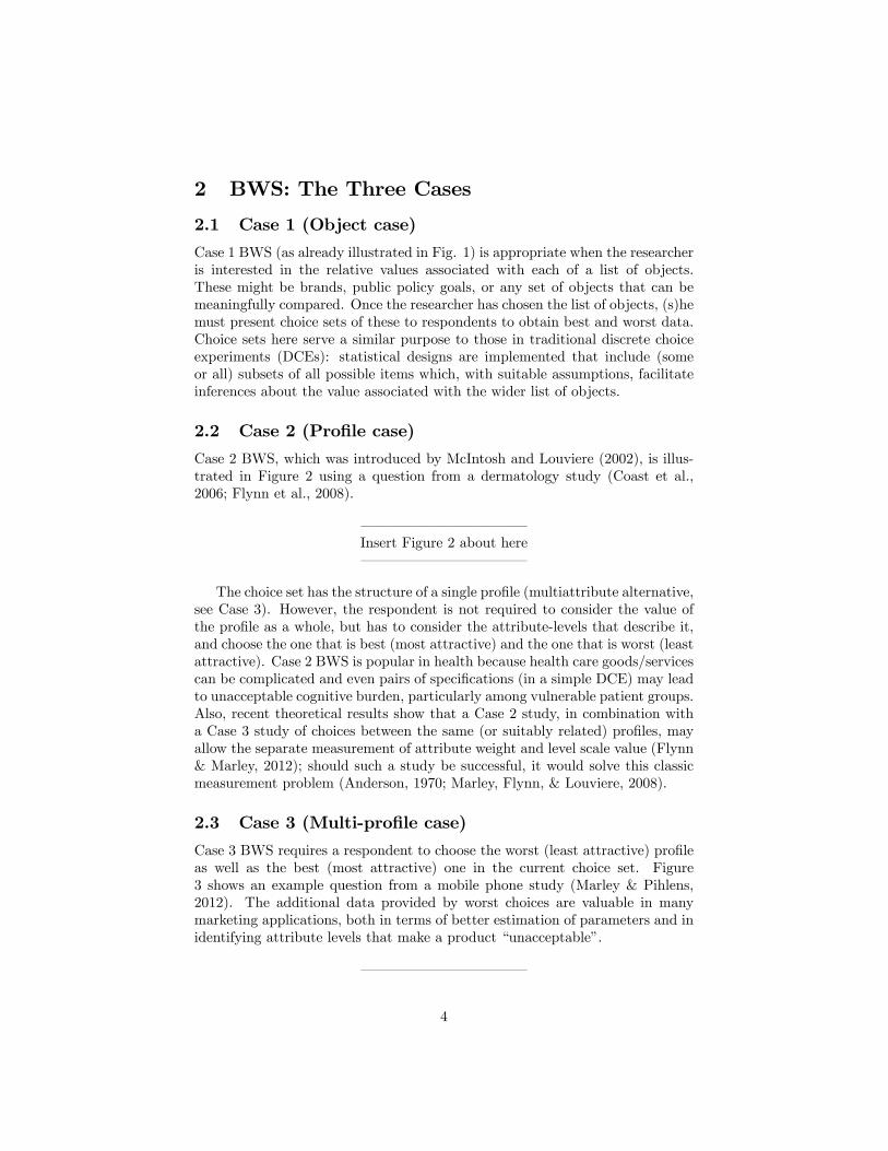
Louviere and Woodworth (1990) and Finn and Louviere (1992) developed a dis-crete choice task in which a person is asked to indicate the “least preferred”itemin a choice set, in addition to indicating the (traditional) “most preferred”item;the approach that Louviere pioneered is now called best worst scaling (BWS).Louviere’s initial focus was on “objects”, such as attitudes, general public policygoals, brands, or anything that did not require a detailed description, such aswould be required for a consumer product such as a soft drink or a car. Thus,Finn & Louviere (1992) used BWS to examine the degree of concern the generalpublic had for each of a set of food safety goals, including irradiation of foodsand pesticide use on crops. Figure 1 contains a BWS question similar to onesused in that study.

– – – – – – – – – – – —Insert Figure 1 about here– – – – – – – – – – – —

Almost immediately, Louviere began applying BWS to more complex itemssuch as attribute-levels describing a single alternative (profile), or complete al-ternatives (profiles) of the type familiar to choice modelers. The former case,requiring respondents to identify the best attribute-level and worst attribute-level within an alternative, was relatively unfamiliar to choice modelers, whereasthe latter case is a “natural”extension of a standard discrete choice experiment(DCE) in which the decision maker selects the most preferred item (Louviere,Hensher & Swait, 2000; Hensher, Rose & Greene, 2005) .BWS was initially used mainly as a method of collecting data in a cost-

effi cient manner, though Finn and Louviere (1992) did introduce the maximumdifference (maxdiff) model for best-worst choice (see below). After a 10-yeardelay, Marley & Louviere (2005) completed an extensive analysis of BWS as atheory, explaining the processes that individuals might follow in providing bestand worst data, and presenting plausible mathematical forms for such processes;summaries of those, and more recent, results are presented in Section 3. Louvierehas recently returned to the use of BWS as a method of data collection (Louviereet al., 2008), in which case its main purpose, via repeated rounds of best-worstchoices, is to obtain a full ranking of items in a manner that is “easy” forrespondents and can then be analyzed in various ways.The remainder of the entry is as follows. Section 2 illustrates the three types

(“cases”) of BWS that Louviere developed. Section 3 summarizes the basicmodels, with Section 3.3 summarizing models of ranking by repeated best and/orworst choices; Section 4 presents properties of simple “scores”; and Section 5summarizes and discusses future research.

3

2 BWS: The Three Cases

2.1 Case 1 (Object case)

Case 1 BWS (as already illustrated in Fig. 1) is appropriate when the researcheris interested in the relative values associated with each of a list of objects.These might be brands, public policy goals, or any set of objects that can bemeaningfully compared. Once the researcher has chosen the list of objects, (s)hemust present choice sets of these to respondents to obtain best and worst data.Choice sets here serve a similar purpose to those in traditional discrete choiceexperiments (DCEs): statistical designs are implemented that include (someor all) subsets of all possible items which, with suitable assumptions, facilitateinferences about the value associated with the wider list of objects.

2.2 Case 2 (Profile case)

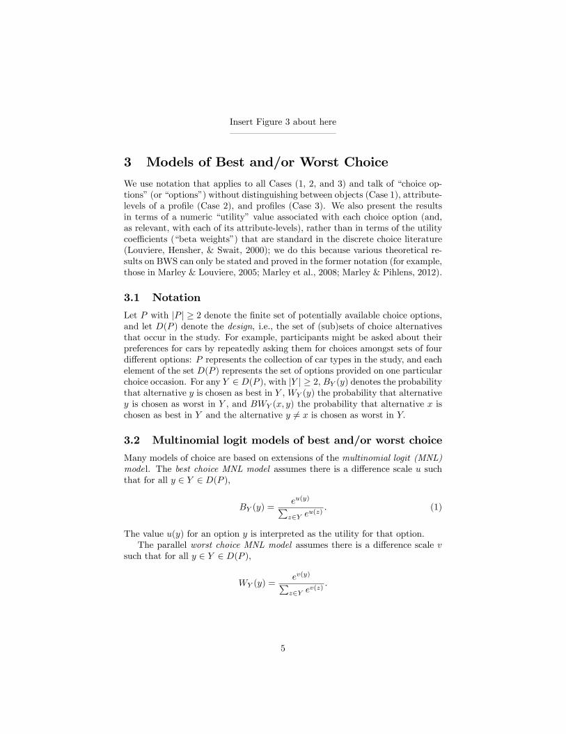
Case 2 BWS, which was introduced by McIntosh and Louviere (2002), is illus-trated in Figure 2 using a question from a dermatology study (Coast et al.,2006; Flynn et al., 2008).

– – – – – – – – – – – —Insert Figure 2 about here– – – – – – – – – – – —

The choice set has the structure of a single profile (multiattribute alternative,see Case 3). However, the respondent is not required to consider the value ofthe profile as a whole, but has to consider the attribute-levels that describe it,and choose the one that is best (most attractive) and the one that is worst (leastattractive). Case 2 BWS is popular in health because health care goods/servicescan be complicated and even pairs of specifications (in a simple DCE) may leadto unacceptable cognitive burden, particularly among vulnerable patient groups.Also, recent theoretical results show that a Case 2 study, in combination witha Case 3 study of choices between the same (or suitably related) profiles, mayallow the separate measurement of attribute weight and level scale value (Flynn& Marley, 2012); should such a study be successful, it would solve this classicmeasurement problem (Anderson, 1970; Marley, Flynn, & Louviere, 2008).

2.3 Case 3 (Multi-profile case)

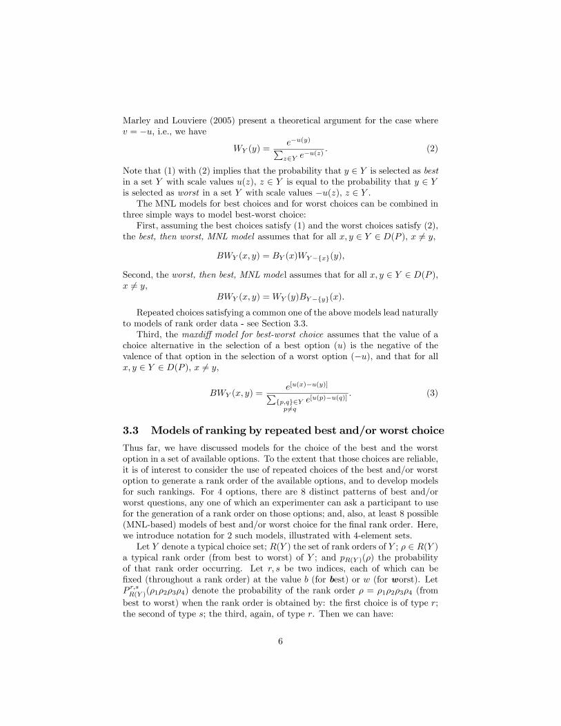
Case 3 BWS requires a respondent to choose the worst (least attractive) profileas well as the best (most attractive) one in the current choice set. Figure3 shows an example question from a mobile phone study (Marley & Pihlens,2012). The additional data provided by worst choices are valuable in manymarketing applications, both in terms of better estimation of parameters and inidentifying attribute levels that make a product “unacceptable”.

– – – – – – – – – – – —

4

Insert Figure 3 about here– – – – – – – – – – – —

3 Models of Best and/or Worst Choice

We use notation that applies to all Cases (1, 2, and 3) and talk of “choice op-tions”(or “options”) without distinguishing between objects (Case 1), attribute-levels of a profile (Case 2), and profiles (Case 3). We also present the resultsin terms of a numeric “utility”value associated with each choice option (and,as relevant, with each of its attribute-levels), rather than in terms of the utilitycoeffi cients (“beta weights”) that are standard in the discrete choice literature(Louviere, Hensher, & Swait, 2000); we do this because various theoretical re-sults on BWS can only be stated and proved in the former notation (for example,those in Marley & Louviere, 2005; Marley et al., 2008; Marley & Pihlens, 2012).

3.1 Notation

Let P with |P | ≥ 2 denote the finite set of potentially available choice options,and let D(P ) denote the design, i.e., the set of (sub)sets of choice alternativesthat occur in the study. For example, participants might be asked about theirpreferences for cars by repeatedly asking them for choices amongst sets of fourdifferent options: P represents the collection of car types in the study, and eachelement of the set D(P ) represents the set of options provided on one particularchoice occasion. For any Y ∈ D(P ), with |Y | ≥ 2, BY (y) denotes the probabilitythat alternative y is chosen as best in Y , WY (y) the probability that alternativey is chosen as worst in Y , and BWY (x, y) the probability that alternative x ischosen as best in Y and the alternative y 6= x is chosen as worst in Y.

3.2 Multinomial logit models of best and/or worst choice

Many models of choice are based on extensions of the multinomial logit (MNL)model. The best choice MNL model assumes there is a difference scale u suchthat for all y ∈ Y ∈ D(P ),

BY (y) =eu(y)∑z∈Y e

u(z). (1)

The value u(y) for an option y is interpreted as the utility for that option.The parallel worst choice MNL model assumes there is a difference scale v

such that for all y ∈ Y ∈ D(P ),

WY (y) =ev(y)∑z∈Y e

v(z).

5

Marley and Louviere (2005) present a theoretical argument for the case wherev = −u, i.e., we have

WY (y) =e−u(y)∑z∈Y e

−u(z) . (2)

Note that (1) with (2) implies that the probability that y ∈ Y is selected as bestin a set Y with scale values u(z), z ∈ Y is equal to the probability that y ∈ Yis selected as worst in a set Y with scale values −u(z), z ∈ Y .The MNL models for best choices and for worst choices can be combined in

three simple ways to model best-worst choice:First, assuming the best choices satisfy (1) and the worst choices satisfy (2),

the best, then worst, MNL model assumes that for all x, y ∈ Y ∈ D(P ), x 6= y,

BWY (x, y) = BY (x)WY−{x}(y),

Second, the worst, then best, MNL model assumes that for all x, y ∈ Y ∈ D(P ),x 6= y,

BWY (x, y) =WY (y)BY−{y}(x).

Repeated choices satisfying a common one of the above models lead naturallyto models of rank order data - see Section 3.3.Third, the maxdiff model for best-worst choice assumes that the value of a

choice alternative in the selection of a best option (u) is the negative of thevalence of that option in the selection of a worst option (−u), and that for allx, y ∈ Y ∈ D(P ), x 6= y,

BWY (x, y) =e[u(x)−u(y)]∑

{p,q}∈Yp 6=q

e[u(p)−u(q)]. (3)

3.3 Models of ranking by repeated best and/or worst choice

Thus far, we have discussed models for the choice of the best and the worstoption in a set of available options. To the extent that those choices are reliable,it is of interest to consider the use of repeated choices of the best and/or worstoption to generate a rank order of the available options, and to develop modelsfor such rankings. For 4 options, there are 8 distinct patterns of best and/orworst questions, any one of which an experimenter can ask a participant to usefor the generation of a rank order on those options; and, also, at least 8 possible(MNL-based) models of best and/or worst choice for the final rank order. Here,we introduce notation for 2 such models, illustrated with 4-element sets.Let Y denote a typical choice set; R(Y ) the set of rank orders of Y ; ρ ∈ R(Y )

a typical rank order (from best to worst) of Y ; and pR(Y )(ρ) the probabilityof that rank order occurring. Let r, s be two indices, each of which can befixed (throughout a rank order) at the value b (for best) or w (for worst). LetP r,sR(Y )(ρ1ρ2ρ3ρ4) denote the probability of the rank order ρ = ρ1ρ2ρ3ρ4 (frombest to worst) when the rank order is obtained by: the first choice is of type r;the second of type s; the third, again, of type r. Then we can have:

6

i. repeated best:

P b,bR(Y )(ρ) = BY (ρ1)BY−{ρ1}(ρ2)B{ρ3,ρ4}(ρ3). (4)

ii. repeated best, then worst:

P b,wR(Y )(ρ) = BY (ρ1)WY−{ρ1}(ρ4)B{ρ2,ρ3}(ρ2). (5)

The natural first assumption in testing these models is to assume that thebest (respectively, worst) choice probabilities satisfy the MNL model (1) (re-spectively, (2)), and, as needed by data, generalizations of those models thatinclude a scale factor that depends on the current choice set in some identifiablemanner; this scale factor relates to the possibly changing variability (“consis-tency”) of the choices across sets. An example of such a generalization of theMNL model for best choices, (1) is: there is a nonnegative scale factor s definedfor each integer 2, 3, .., and a difference scale u such that for all y ∈ Y,

BY (y) =es(|Y |)u(y)∑z∈Y e

s(|Y |)u(z) . (6)

We then define a generalized rank ordered logit model (GROL) as a set of rankorders that satisfy (4) with the best choice probabilities satisfying (6). Theform (6) is a special case of what Vermunt and Magidson (2005, Section 2.4)call an MNL with replication-specific scale factor and of Fiebig et al.’s (2010)generalized multinomial logit model (GMNL); the latter model also includes scale(variance) heterogeneity across individuals.Scarpa, Notaro, Raffelli, Pihlens, and Louviere (2011) collected ranking data

by repeated best, then worst, choices and fit that data quite successfully witha model based on repeated best choice, i.e. (4), with those choices satisfying ageneralization of the model in (6) that included properties of the scale factor son aspects of the design that took account of the difference between the datacollection method (repeated best, then worst) and the model (repeated best);it would be interesting to see if their data could be better fit by a model thatmatched their data collection method, i.e. (5). Collins and Rose (2011) fitrelated models to stated preference data on dating choices.

3.4 Maximum random utility models of choice and re-sponse time

When treated as a single model, the three models (1), (2), and (3), satisfyan inverse extreme value maximum random utility model (Marley & Louviere,2005, Def. 11). That is, for z ∈ P and p, q ∈ P , p 6= q, there are independentrandom variables εz, εp,q with the extreme value distribution1 such that for ally ∈ Y ∈ D(P ),

BY (y) = Pr

(u(y) + εy = max

z∈Y[u(z) + εz]

), (7)

1This means that: for −∞ < t <∞ Pr(εz ≤ t) = exp−e−t and Pr(εp,q ≤ t) = exp−e−t.

7

WY (y) = Pr

(−u(y) + εy = max

z∈Y[−u(z) + εz]

), (8)

and for all x, y ∈ Y ∈ D(P ), x 6= y,

BWY (x, y) = Pr

u(x)− u(y) + εx,y = maxp,q∈Yp 6=q

[u(p)− u(q) + εp,q]

. (9)

Standard results (summarized by Marley & Louviere, 2005) show that the ex-pression for the choice probabilities given by (7) (respectively, (8), (9)) agreeswith that given by (1) (respectively, (2), (3)).These random utility models are particularly interesting in the present con-

text because they can be rewritten, and extended, in such a way as to alsopredict response time (Hawkins et al., 2012).

3.5 Extensions of the models to Case 2 and Case 3

The notation, models, and results (such as for scores, Section 4) are easilyextended to Case 2 and Case 3 - see Marley, et al. (2008) for Case 2, Marleyand Pihlens (2012) for Case 3, and Flynn and Marley (2012) for a summary ofall cases.

4 Properties and Uses of Scores for the MaxdiffModel

We now summarize theoretical and empirical results for best minus worst scores(defined below) for the maxdiff model of best-worst choice. Although the theo-retical results are not exact for, say, the best, then worst, MNL model, to dateno identifiable differences have been found between fits of that model and themaxdiff model (see Flynn et al., 2008, for an example of such fits); hence thescore measures are useful for preliminary analyses of the data independent ofthe model that is eventually fit to the data.For each option x in the design, the score for x (in this particular design) is

the number of times option x is chosen as best in the study minus the numberof times option x is chosen as worst in the study; we call refer to “the scores”for these values across the options in the design.Scores: Theoretical Property 1 (for Case 1, 2, and 3)Marley and Islam (2012) state the following terms and results exactly. As-

sume that one is interested in the rank order, only, of the (utility) scale valuesin the maxdiff model. An acceptable loss function is a “penalty”function witha value that remains constant under a common permutation of the scores andthe scale values, and that increases if the ranking is made worse by misorderinga pair of scale values. Let P be a master set with n ≥ 2 elements and assumethat, for some k with n ≥ k ≥ 2, every subset of P with exactly k elements

8

appears in the design2 D(P ). Then, given the maxdiff model, ranking the scalevalues in descending order of the (best minus worst) scores, breaking ties at ran-dom, has “minimal average loss”amongst all (“permutation invariant”) rankingprocedures that depend on the data only through the set of scores.The above result actually holds for the class of weighted utility ranking mod-

els, which includes the MNL for best; MNL for worst; and the maxdiff modelfor best-worst choice (Marley & Islam, 2012).Scores: Theoretical Property 2 (for Case 1, 2 and 3)The set of (best minus worst) scores is a suffi cient statistic. As with the

first theoretical property, this one holds for the class of weighted utility rankingmodels (Marley & Islam, 2012, Theorem 3).Scores: Empirical Properties (for Case 1, 2 and 3)The best minus worst scores have been found to be linearly related to the

maximum likelihood estimates of the best, then worst, MNL model, and of themaxdiff model, in virtually every empirical study to date. For example, Flynn(2010) obtained this result in a Case 2 quality of life study, and Marley andIslam (2012) present such linear relations for both profiles and attribute-levelsin a Case 3 study of consumer attitudes to the installation of solar technologyfor household electricity production. Such linearity is probably a manifestationof the linear portion of the logistic (cumulative distribution) function; thus, anon-linear relationship is likely only when the researcher is plotting the scoresfor a single highly consistent respondent, or for a sample of respondents eachof whom is highly consistent and the choices are highly consistent across thesample.The scores also enable considerable insights to be drawn at the level of the

individual respondent. For example taxonomic (clustering) methods of analysishave been applied to the scores (Auger et al., 2007) and Flynn and colleagueshave used the scores to decide which solutions from latent class analyses “makesense”(Flynn et al., 2010).

5 Summary and Future Research

Further research is needed to understand the factors affecting the scale factor atdifferent choice depths and the conditions under which the data require differentfunctional forms (models) for best and worst choices. Also, research to datesuggests that the class of models with natural process interpretations is differentfrom the class of models with useful score properties. Nonetheless, the scoresmay give the average applied researcher more confidence, not least in terms ofbetter understanding heterogeneity in preferences and/or scale factors in theirdata.Data pooling has normative issues that are particularly pertinent to health

economists: for best-worst choice, it is only if all individuals satisfy the maxdiffmodel that the average of their utility estimates represents the preferences of

2Further work is needed to extend the theoretical result to, say, balanced incomplete block(BIBD) designs. See Marley & Pihlens (2012) for related discussions of connected designs.

9

the “representative individual”used in economic evaluation. Also, appropriatedata pooling exercises (likely involving Case 2 and Case 3 data) may allow theseparation of attribute weight and level scale value (Marley, Flynn, & Louviere2008; Flynn & Marley, 2012). While the distinction between these two measuresis not recognized by traditional economic welfare theory, it offers benefits tohealth researchers constructing multi-dimensional health outcome instrumentsfrom individual symptom scales: for example, rejection of a simple “sum-score”aggregation rule necessitates decisions as to what importance weights are to beapplied to the individual symptom scales (Fayers & Machin, 2007, p.218).

Acknowledgements

This research has been supported by Natural Science and Engineering Re-search Council Discovery Grant 8124-98 to the University of Victoria for Marley.The work was carried out, in part, whilst Marley was a Distinguished ResearchProfessor (part-time) at the Centre for the Study of Choice, University of Tech-nology Sydney.

References

Anderson, N. H. (1970). Functional measurement and psychophysical judge-ment. Psychological Review, 77(3), 153-170.Auger, P., Devinney, T. M., & Louviere, J. J. (2007). Using best-worst

scaling methodology to investigate consumer ethical beliefs across countries.Journal of Business Ethics, 70, 299-326.Coast, J., Salisbury, C., de Berker, D., Noble, A., Horrocks, S., Peters, T. J.,

& Flynn, T. N. (2006). Preferences for aspects of a dermatology consultation.British Journal of Dermatology, 155, 387-392.Collins, A. T., & Rose, J. M. (2011). Estimation of a stochastic scale with

best-worst data. Paper presented at the Second International Choice ModellingConference, Leeds, UK.Fayers, P. M. & Machin, D. (2007). Quality of Life: The Assessment, Analy-

sis and Interpretation of Patient-reported Outcomes. Chichester, John Wiley.Fiebig, D. G., Keane, M. P., Louviere, J., &Wasi, N. (2010). The generalized

multinomial logit model: Accounting for scale and coeffi cient heterogeneity.Marketing Science, 29, 393-421Finn, A., & Louviere, J. J. (1992). Determining the appropriate response to

evidence of public concern: The case of food safety. Journal of Public Policy &Marketing, 11, 12-25.

Flynn T. N. (2010). Valuing citizen and patient preferences in health: recentdevelopments in three types of best-worst scaling. Expert Review of Pharma-coeconomics & Outcomes Research, 10, 259-267.

Flynn, T. N. & Marley, A. A. J. (2012). Best-worst scaling: theory andmethods. Invited chapter in S. Hess & A. Daly (Eds.) Handbook of ChoiceModelling. Edward Elgar Publishing. Submitted.

10

Flynn, T. N., Louviere, J. J., Peters, T. J., & Coast, J. (2008). Estimatingpreferences for a dermatology consultation using Best-Worst Scaling: Compari-son of various methods of analysis. BMC Medical Research Methodology, 8(76).Flynn, T. N., Louviere, J. J., Peters, T. J., & Coast, J. (2010). Using dis-

crete choice experiments to understand preferences for quality of life. Variancescale heterogeneity matters. Social Science & Medicine, 70, 1957-1965. doi:doi:10.1016/j.socscimed.2010.03.008Hawkins, G. E., Marley, A. A. J., Heathcote, A., Flynn, T. N., Louviere,

J. J., & Brown, S. D., (2012). Accumulator models for best-worst choices. De-partment of Psychology. University of Newcastle, Australia. Newcastle, NSW,Australia.Hensher, D. A., Rose, J. M., & Greene, W. H. (2005). Applied choice analy-

sis: a primer. Cambridge: Cambridge University Press.Huber, P. J. (1963). Pairwise comparison and ranking: optimum properties

of the row sum procedure. Annals of Mathematical Statistics, 34, 511-520.Louviere, J. J., Hensher, D. A., & Swait, J. D. (2000). Stated Choice Meth-

ods. Cambridge: Cambridge University Press.Louviere, J. J., & Street, D. (2000). Stated preference methods. In D. A.

Hensher & K. Button (Eds.), Handbook in Transport I: Transport Modelling.(pp. 131-144). Amsterdam: Pergamon (Elsevier Science).Louviere, J. J., Street, D. J., Burgess, L., Wasi, N., Islam, T., & Marley, A.

A. J. (2008). Modelling the choices of single individuals by combining effi cientchoice experiment designs with extra preference information. Journal of ChoiceModelling, 1, 128-163.Marley, A. A. J., Flynn, T. N., & Louviere, J. J. (2008). Probabilistic models

of set-dependent and attribute-level best-worst choice. Journal of MathematicalPsychology, 52, 281-296.

Marley, A. A. J., & Islam, T. (2012). Conceptual relations between ex-panded rank data and models of the unexpanded rank data. Journal of ChoiceModelling. In Press.Marley, A. A. J., & Louviere, J. J. (2005). Some probabilistic models of

best, worst, and best-worst choices. Journal of Mathematical Psychology, 49,464-480.Marley, A. A. J., & Pihlens, D. (2012). Models of best-worst choice and

ranking among multi-attribute options (profiles). Journal of Mathematical Psy-chology, 56, 24-34.McIntosh, E., & Louviere, J. J. (2002). Separating weight and scale value:

an exploration of best-attribute scaling in health economics. Health Economists’Study Group, Brunel University.Scarpa, R., Notaro, S., Raffelli, R., Pihlens, D., & Louviere, J. J. (2011).

Exploring scale effects of best/worst rank ordered choice data to estimate ben-efits of tourism in alpine grazing commons. American Journal of AgriculturalEconomics, 93, 813-828.Vermunt, J. K., & Magidson, J. (2005). Technical Guide for Latent GOLD

Choice 4.0: Basic and Advanced. Belmont Massachusetts: Statistical Innova-tions.

11

Figure 1. A completed example BWS ‘object case’ question

Most Issue Least Pesticides used on crops Hormones given to livestock Irradiation of foods Excess salt, fat cholesterol

Antibiotics given to livestock

Please consider the food safety issues in the table above and tick which concerns you most and which concerns you least.

12

Figure 2. A completed example BWS ‘profile case’ question

Most Appointment #1 Least You will have to wait two months for your appointment The specialist has been treating skin complaints part-time for 1-2 years Getting to your appointment will be quick and easy

The consultation will be as thorough as you would like

Please imagine being offered the appointment described above and tick which feature would be best and which would be worst.

13

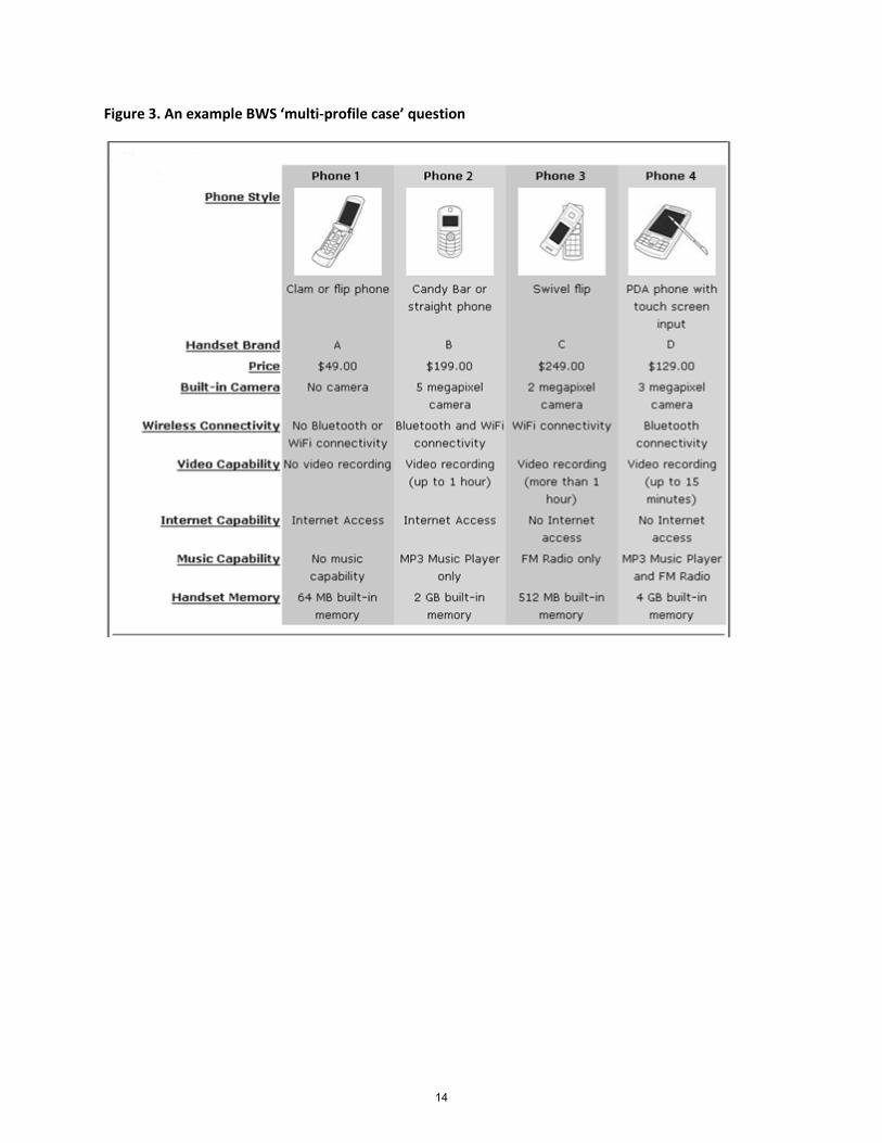
Figure 3. An example BWS ‘multi-profile case’ question

14

Website Citations Centre for the Study of Choice http://www.censoc.uts.edu.au/ Journal of Choice Modelling http://www.jocm.org.uk/index.php/JOCM Society for Judgment and Decision Making http://www.sjdm.org/ Daniel L. McFadden http://emlab.berkeley.edu/~mcfadden/ T. N. Flynn http://datasearch.uts.edu.au/censoc/members/detail.cfm?StaffID=7884 J. Louviere htttp://datasearch.uts.edu.au/censoc/members/detail.cfm?StaffID=158 A. A. J. Marley http://www.uvic.ca/psyc/marley/ Cross References to Related Entries in the Encyclopedia Note to the Editors: These are only for Section 4. We do not know how to access other sections (such as those on Economics and Medicine) 41028. Experimental Laboratories: Biobehavioral, Neuroscientific, Psychological 41029 Experimental Laboratories: Social and Economic 43031. Decision and Choice: Luce's Choice Axiom 43033. Decision and choice: random utility models of choice and response time 43035. Decision and choice: utility and subjective probability, empirical studies 43060. Measurement Theory: Conjoint Analysis Applications 43063. Measurement theory: probabilistic 43082. Psychometrics: Preference Models with Latent Variables 43094. Stochastic dynamic models (choice, response, time) 43108. Decision and Choice: Risk, Empirical Studies 43109. Decision and Choice: Risk, Theories 44040. Panel Surveys, Uses and Applications

15