All views expressed in this paper are those of the authors and do not necessarily represent the views of the Hellenic Observatory or the LSE © Vassilis Monastiriotis and Angelo Martelli

Beyond Rising Unemployment:

Unemployment Risk, Crisis and Regional

Adjustments in Greece

Vassilis Monastiriotis and Angelo Martelli

GreeSE Paper No.80

Hellenic Observatory Papers on Greece and Southeast Europe

DECEMBER 2013

ii

_

TABLE OF CONTENTS

ABSTRACT __________________________________________________________ iii

1. Introduction _____________________________________________________ 1

2. Data and method _________________________________________________ 5

3. Unemployment risk in the Greek regions _____________________________ 11

3.1 ‘Baseline’ unemployment risk __________________________________ 12

3.2 Unemployment risk and education ______________________________ 16

3.3 Unemployment risk for other characteristics ______________________ 20

4. Decomposition analysis: macro-geographies of unemployment ___________ 27

5. Conclusions _____________________________________________________ 38

APPENDIX __________________________________________________________ 43

References _________________________________________________________ 49

iii

Beyond Rising Unemployment:

Unemployment Risk, Crisis and Regional

Adjustments in Greece

Vassilis Monastiriotis # and Angelo Martelli

ABSTRACT

The remarkable rise in unemployment in Greece has in a way overshadowed the substantial differentiation, across regions, in terms of regional unemployment and labour market adjustment. This paper examines the geography of these dynamics using probit regressions of unemployment risk and decomposing the observed regional unemployment differentials into three components corresponding to differences in labour quality, matching efficiency and effective demand. We find that, underlying the general increase in unemployment is a wealth of unemployment dynamics and adjustment trajectories. The fall in effective demand has been largest in the main metropolitan regions and the north and north-western periphery. Adjustment has been strong in some areas (e.g., Athens) but, overall, adjustment processes (such as bumping-down and changes in the mix of workforce characteristics) have been weak. The crisis has nullified the improvements in labour market performance registered since the country’s entry into the Eurozone, hitting especially those regions that benefitted most from the latter. The spatial differentiation of adjustment intensities and demand pressures suggests a heightened role for regional policy in the post-crisis period, especially in relation to addressing problems of over-education and matching efficiency in the demand-depressed areas and of inter-regional adjustment mechanisms nationally.

#Associate Professor in the Political Economy of South East Europe, London School of Economics Phd candidate, European Institute,London School of Economics

1

1

Beyond Rising Unemployment:

Unemployment Risk, Crisis and Regional

Adjustments in Greece

1. Introduction

As is well documented, unemployment in Greece has increased

immensely during the last four years, reaching over 27% by early 2013.

In many respects this increase has been universal, affecting all regions in

a broadly similar fashion, as the shock that instigated it (the Greek fiscal

crisis) was exogenous to the regions and seemingly symmetric (for

evidence against this, see Monastiriotis, 2011). At a closer inspection,

however, some notable heterogeneity emerges with regard to regional

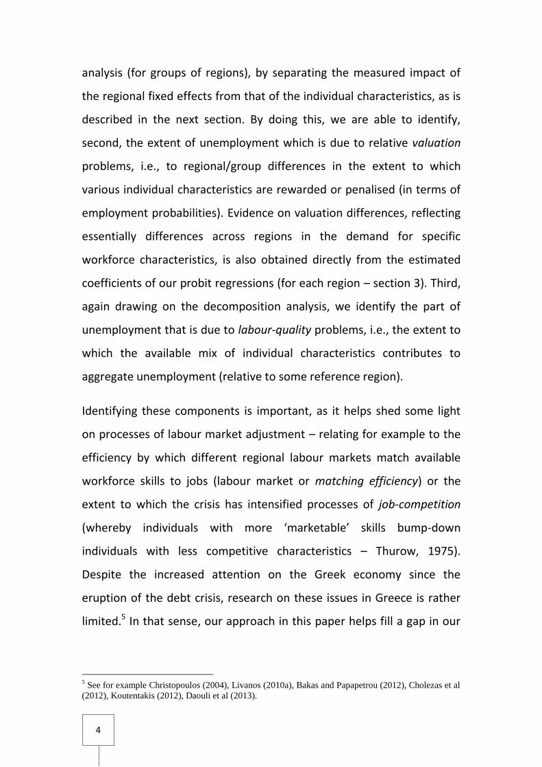
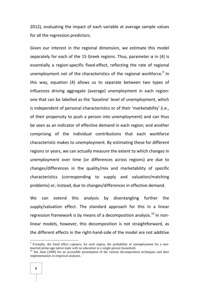
unemployment evolutions (see Fig.1). In 2012, unemployment rates

ranged between less than 15% in the Ionian and over 30% in Western

Macedonia. Moreover, between 2008 and 2012 unemployment rates

increased by a ‘low’ 140% (or less) in the regions of Ipeiros, Ionian,

Western Macedonia and South Aegean; but by multiples of this (over

300%) in Crete, Athens and the North Aegean. Curiously, membership

into these groups is not easy to interpret. For example, the ‘low-rise’

group includes the region with the highest unemployment rate in the

country (Western Macedonia), both historically and in 2012, as well as

two regions that have had historically among the lowest unemployment

rates nationally (Ionian and South Aegean). Similarly, the ‘high-rise’

group includes a large metropolitan area (Athens), a less dense but

2

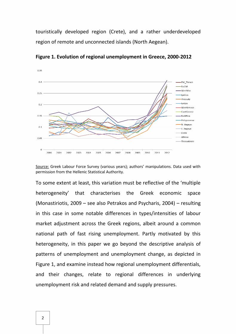
touristically developed region (Crete), and a rather underdeveloped

region of remote and unconnected islands (North Aegean).

Figure 1. Evolution of regional unemployment in Greece, 2000-2012

Source: Greek Labour Force Survey (various years); authors’ manipulations. Data used with permission from the Hellenic Statistical Authority.

To some extent at least, this variation must be reflective of the ‘multiple

heterogeneity’ that characterises the Greek economic space

(Monastiriotis, 2009 – see also Petrakos and Psycharis, 2004) – resulting

in this case in some notable differences in types/intensities of labour

market adjustment across the Greek regions, albeit around a common

national path of fast rising unemployment. Partly motivated by this

heterogeneity, in this paper we go beyond the descriptive analysis of

patterns of unemployment and unemployment change, as depicted in

Figure 1, and examine instead how regional unemployment differentials,

and their changes, relate to regional differences in underlying

unemployment risk and related demand and supply pressures.

3

3

To perform this analysis, we adopt a micro-econometric approach and

look at the incidence and determinants of unemployment risk across the

Greek regions1 using probit regressions on individual-level data derived

from the Greek Labour Force Survey covering the period 2000-2012.

Following Lopez-Bazo and Motellon (2013)2 we further apply an

unemployment-risk decomposition analysis across groups of regions of

different structural, economic and locational characteristics for periods

before and during the crisis, in order to examine how different types of

regional labour markets have responded to the crisis.

Examining unemployment risk in this way allows us to identify a number

of distinctive influences exerted on the regional labour markets of

Greece, which may be hard to unveil in an aggregate-level analysis.3

First, using the regional fixed-effects from the probit regressions, we

derive a measure of unemployment that is net of personal

characteristics and of the unemployment risk assigned to each of these

individually (expressed in terms of a ‘baseline’ worker profile that is

common in all regions and years). We interpret this as a measure of

effective demand4 for each regional labour market – and variations in

this as a measure of the relative intensity of the demand shock

experienced by each regional labour market under the crisis. We also

derive a measure of relative demand through our decomposition

1 We use the 15 statistical regions reported in the Greek LFS comprising the 13 NUTS2 regions, with

the metropolitan areas of Athens (part of the NUTS2 region of Attiki) and Thessaloniki (part of Central

Macedonia) reported separately. 2 For an earlier implementation of the decomposition approach, examining differences across ethnic

groups, see Blackaby et al (1999). 3 Elhorst (2003) discusses the limitations of aggregate-level analyses of unemployment in the absence

of good-quality regional data and ‘perfect knowledge’ about the correct model describing intra- and

inter-regional labour market dynamics. 4 Evidently, this measure is imperfect as it is not independent of our choice of reference categories in

the probit regressions – although the use of a fixed reference category over time and across space

makes it appropriate for cross-regional and temporal comparisons.

4

analysis (for groups of regions), by separating the measured impact of

the regional fixed effects from that of the individual characteristics, as is

described in the next section. By doing this, we are able to identify,

second, the extent of unemployment which is due to relative valuation

problems, i.e., to regional/group differences in the extent to which

various individual characteristics are rewarded or penalised (in terms of

employment probabilities). Evidence on valuation differences, reflecting

essentially differences across regions in the demand for specific

workforce characteristics, is also obtained directly from the estimated

coefficients of our probit regressions (for each region – section 3). Third,

again drawing on the decomposition analysis, we identify the part of

unemployment that is due to labour-quality problems, i.e., the extent to

which the available mix of individual characteristics contributes to

aggregate unemployment (relative to some reference region).

Identifying these components is important, as it helps shed some light

on processes of labour market adjustment – relating for example to the

efficiency by which different regional labour markets match available

workforce skills to jobs (labour market or matching efficiency) or the

extent to which the crisis has intensified processes of job-competition

(whereby individuals with more ‘marketable’ skills bump-down

individuals with less competitive characteristics – Thurow, 1975).

Despite the increased attention on the Greek economy since the

eruption of the debt crisis, research on these issues in Greece is rather

limited.5 In that sense, our approach in this paper helps fill a gap in our

5 See for example Christopoulos (2004), Livanos (2010a), Bakas and Papapetrou (2012), Cholezas et al

(2012), Koutentakis (2012), Daouli et al (2013).

5

5

understanding of the prevalence of such processes in the Greek

economy.

The remainder of the paper is structured as follows. In the next section

we describe our micro-econometric approach and the decomposition

technique used to derive the distinct components of unemployment.

Section 3 presents the results from our analysis of unemployment risk

across the Greek regions, focusing in particular on the spatial

differentiation in terms of unemployment risk for specific individual

characteristics (age, gender, education, etc). In section 4 we shift our

focus to the macro-geographies of unemployment in Greece and

examine, through our decomposition analysis, the direction of relative

labour market adjustments across different regional groupings. Section 5

concludes with some implications for policy, particularly on the scope

and priorities of (future) regional policy in Greece.

2. Data and method

As mentioned previously, our approach departs from the analysis of

aggregate unemployment and seeks to investigate the dynamics of

regional unemployment with the use of individual-level data within the

context of unemployment-risk probit regressions. The essence of this

approach is similar to that applied widely in the wage-equations

literature6: in our case, unemployment status is determined by an

unobserved latent variable (of a continuously-distributed underlying

unemployment risk), which is in turn dependent on a set of personal

6 See Heckman et al (2006) for a review of the so-called Mincer wage equation model.

6

characteristics (plus an area fixed-effect, capturing the overall market

conditions in each regional labour market). Formally,

iii bXU *

(1)

where is the unobserved (latent) variable measuring the

unemployment risk of individual i, is a vector of personal and other

characteristics of that individual, is a vector of parameters measuring

the contribution of each individual characteristic to unemployment risk

and εi is a normally distributed person-specific disturbance. The

observed unemployment status U is linked to this latent variable by the

following condition:

(2)

Under these conditions, the probability of observing U=1 (i.e., someone

being unemployed) is equal to the standard normal cumulative

distribution for and thus the parameter can be estimated by means

of a probit regression as

(3)

where is the inverse of the standard normal cumulative distribution.

This is a model that has been used widely in the literature to examine

various issues concerning the incidence and determinants of

unemployment, including the contribution to unemployment of various

individual (education – Ashenfelter and Ham, 1979) and family

characteristics (family size – McGregor, 1978); the impact on

unemployment of various policy variables (e.g., unemployment benefits

7

7

– Solon, 1979); issues of labour market discrimination (Stratton, 1993)

and migrant assimilation (McDonald and Worswick, 1997); and many

others.7

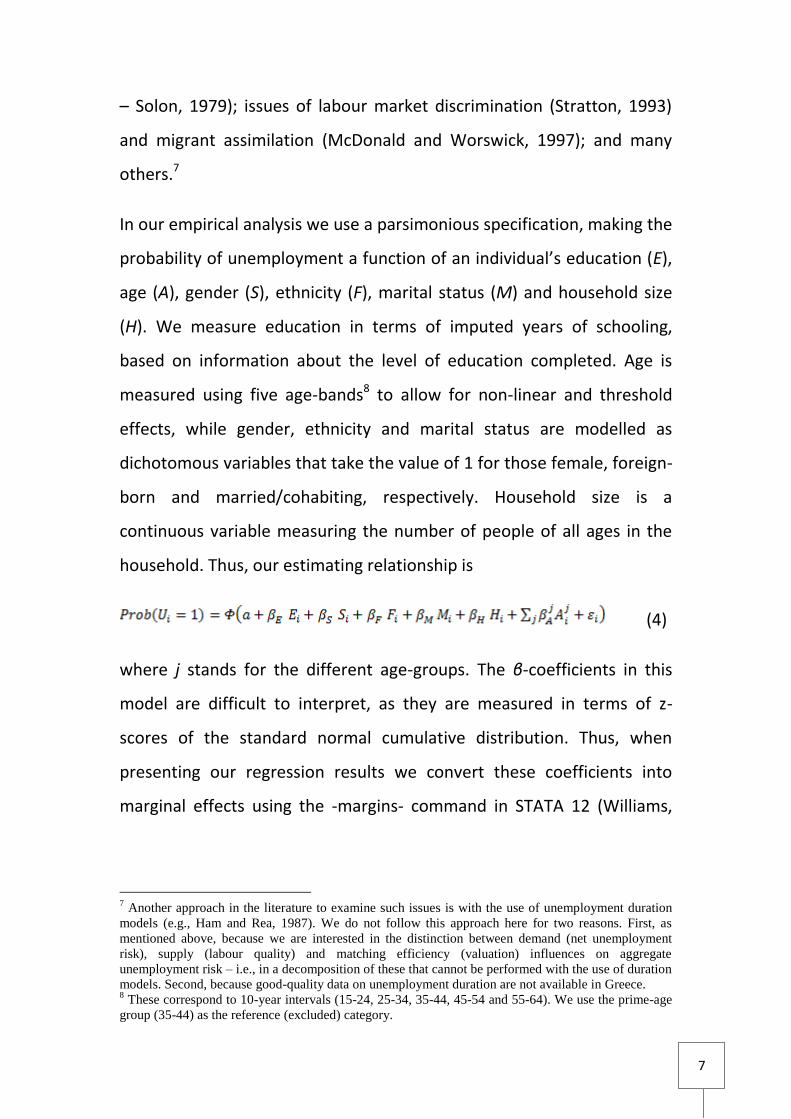
In our empirical analysis we use a parsimonious specification, making the

probability of unemployment a function of an individual’s education (E),

age (A), gender (S), ethnicity (F), marital status (M) and household size

(H). We measure education in terms of imputed years of schooling,

based on information about the level of education completed. Age is

measured using five age-bands8 to allow for non-linear and threshold

effects, while gender, ethnicity and marital status are modelled as

dichotomous variables that take the value of 1 for those female, foreign-

born and married/cohabiting, respectively. Household size is a

continuous variable measuring the number of people of all ages in the

household. Thus, our estimating relationship is

(4)

where j stands for the different age-groups. The β-coefficients in this

model are difficult to interpret, as they are measured in terms of z-

scores of the standard normal cumulative distribution. Thus, when

presenting our regression results we convert these coefficients into

marginal effects using the -margins- command in STATA 12 (Williams,

7 Another approach in the literature to examine such issues is with the use of unemployment duration

models (e.g., Ham and Rea, 1987). We do not follow this approach here for two reasons. First, as

mentioned above, because we are interested in the distinction between demand (net unemployment

risk), supply (labour quality) and matching efficiency (valuation) influences on aggregate

unemployment risk – i.e., in a decomposition of these that cannot be performed with the use of duration

models. Second, because good-quality data on unemployment duration are not available in Greece. 8 These correspond to 10-year intervals (15-24, 25-34, 35-44, 45-54 and 55-64). We use the prime-age

group (35-44) as the reference (excluded) category.

8

2012), evaluating the impact of each variable at average sample values

for all the regression predictors.

Given our interest in the regional dimension, we estimate this model

separately for each of the 15 Greek regions. Thus, parameter α in (4) is

essentially a region-specific fixed-effect, reflecting the rate of regional

unemployment net of the characteristics of the regional workforce.9 In

this way, equation (4) allows us to separate between two types of

influences driving aggregate (average) unemployment in each region:

one that can be labelled as the ‘baseline’ level of unemployment, which

is independent of personal characteristics or of their ‘marketability’ (i.e.,

of their propensity to push a person into unemployment) and can thus

be seen as an indicator of effective demand in each region; and another

comprising of the individual contributions that each workforce

characteristic makes to unemployment. By estimating these for different

regions or years, we can actually measure the extent to which changes in

unemployment over time (or differences across regions) are due to

changes/differences in the quality/mix and marketability of specific

characteristics (corresponding to supply and valuation/matching

problems) or, instead, due to changes/differences in effective demand.

We can extend this analysis by disentangling further the

supply/valuation effect. The standard approach for this in a linear

regression framework is by means of a decomposition analysis.10 In non-

linear models, however, this decomposition is not straightforward, as

the different effects in the right-hand-side of the model are not additive

9 Formally, the fixed effect captures, for each region, the probability of unemployment for a non-

married prime-age native male with no education in a single-person household. 10

See Jann (2008) for an accessible presentation of the various decomposition techniques and their

implementation in empirical analyses.

9

9

and thus the conditional expectation of the dependent variable will not

be equal to the regression prediction at mean sample values.11 An early

solution to this problem was proposed by Gamulka and Stern (1990) for

the aggregate decomposition, while more recent contributions have

allowed also the implementation of variable-specific decompositions

(Yun, 2004) as well as decompositions of the imputed marginal effects

(Fairlie, 2005).

The decomposition approach in these cases follows the same logic as the

standard Blinder-Oaxaca decomposition for linear models. Starting from

the general model presented in (3), we calculate average group-specific

unemployment probabilities for two different groups, say regions A and

B, and decompose their differences as follows:

(6)

where the bar above each term denotes sample averages. As in the

standard Blinder-Oaxaca decomposition, the first bracket on the right-

hand side gives the difference in average unemployment between

regions A and B which is due to differences in workforce characteristics;

while the second bracket gives the part of the unemployment

differential that is due to differences in the value attached to the various

characteristics.

As with the linear decomposition, these components can be ‘evaluated’

at different reference values. The decomposition shown in (6)

corresponds to the standard Blinder-Oaxaca approach, whereby

‘endowments’ are evaluated at region A coefficients while the

11

Formally, . See Bauer and Sinning (2008) for a discussion of this.

10

‘coefficients’ component is measured on the basis of region B

characteristics. Other decompositions are also possible: for example, the

pooled-estimate decomposition (Neumark, 1988) can also be adapted

for the case of non-linear models, allowing the ‘endowment’ effect to be

expressed in terms of full-sample coefficients.12 The same applies for the

case of the three-way decomposition proposed by Daymont and

Andrisani (1984), which separates between an ‘endowment’, a ‘price’

and an ‘interaction’ effect.

Implementing any of these decompositions is useful, but in relation to

our earlier discussion it imposes a crucial problem: the price effect

derived from such aggregate decompositions includes the contribution

to regional unemployment differentials of the region-specific fixed-

effects. This prohibits us from distinguishing between ‘effective demand’

(fixed-effect) and ‘valuation’ influences (‘coefficients’ effect for

individual-specific characteristics). To overcome this problem, we need

to revert to a variable-specific decomposition. A method for this, in the

case of non-linear models, was proposed by Yun (2004) and is

implemented in STATA using the -oaxaca- command developed by Jann

(2008). The method also performs a correction for the ‘decomposition

identification problem’ (Oaxaca and Ransom, 1999; Yun, 2005).13 With

the use of this technique, we are able to decompose any observed

unemployment differential between two groups of regions into three

12

In that case, the ‘price’ effect is essentially measured as the difference between average

characteristics in A valuated in terms of the price advantage in A relative to the full sample and the

average characteristics in B valuated in terms of the analogous price advantage in B. 13

The problem arises in models that include dichotomous variables as regressors, as the value of the

estimated intercept becomes dependent on the reference category selected. The technique used here

(Yun, 2005) corrects for this by essentially averaging out across estimates derived from the use of

alternative reference categories. As a result, the estimated fixed-effects become independent of the

choice of reference categories for the dichotomous variables, allowing their interpretation here as

measures of effective demand (in this case, irrespective of the ‘baseline’ profile).

11

11

distinctive components: one capturing differences in labour quality (the

‘endowment’ or ‘explained’ component); one capturing differences in

the valuation of marketable characteristics and thus in the mix of

attributes (e.g., skill-content) demanded in each labour market (the sum

of the individual variable-specific ‘coefficient’ components); and one

capturing differences in effective demand across the two groups of

regions (the estimated variable-specific ‘coefficient’ component

corresponding to the fixed-effect).

With this “technology”, we set out to explore the questions elaborated

earlier, concerning the sources of unemployment in Greece and their

regional differentiation before and during the crisis. In the empirical

analysis that follows we use data from the spring-quarter waves of the

Greek labour force survey for the years 2000-2012. We derive

information on the range of individual and family characteristics

depicted in equation (4) and restrict our sample to working-age

respondents who were either employed or had actively looked for a job

in the two weeks prior to the survey. After some data cleaning, the

typical year contains some 30,000-35,000 observations.14 Some basic

descriptive statistics for our key variables (for selected years) are

presented in the Appendix.

3. Unemployment risk in the Greek regions

The first task in our analysis is to measure the individual contribution of

various personal and household characteristics to unemployment risk

and their differentiation over time and across space. With over half a

14

The number of observations in the Greek Labour Force Survey declines in more recent years. In

2012, our effective sample includes just over 25,000 observations.

12

dozen such characteristics evaluated across 15 regions over a 13-year

period (2000-2012), the number of estimated coefficients that we are

potentially interested in exceeds 1,500. To facilitate presentation and

discussion, we make use of GIS tools and present a number of maps

where we depict, for each variable of interest, the corresponding

marginal effect derived for each of the 15 regions of Greece over two

periods: before (2005-2008) and during the crisis (2009-2012). Full tables

of results for all 15 regions for selected years (2000, 2004, 2008 and

2012) reporting marginal effects are given in the Appendix.15 We make

selective reference to region- and year-specific estimates in the text,

where relevant. Overall, our probit regressions perform well, with the

Wald statistic testing for the validity of the model being always

significant at even the 0.1% and an average value for the McFadden

pseudo R-squared of 0.12.

3.1 ‘Baseline’ unemployment risk

Starting with the region-specific fixed effects, we note that these are

always statistically significant and negative in the early periods,

indicating low ‘baseline’ probabilities of unemployment before the crisis

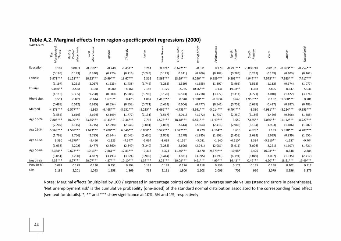
(see Table A.2 and Figure 2), but become statistically weaker and

sometimes even positive during the crisis. In 2000, the estimated fixed-

effects range from -0.84 to -2.58, corresponding to ‘net’ unemployment

rates16 of between 0.5% (in the South Aegean) and 20% (in Western

Macedonia) – with the two main metropolitan areas (Athens and 15

Direct regression estimates (z-score coefficients) and full results for all years can be made available

upon request. 16

Net unemployment rates deriving from the fixed effects have been calculated using the one-sided

cumulative function of the standard normal distribution. As noted already, these rates should not be

seen as absolute measures of effective demand but rather as the unemployment-risk probabilities

corresponding to our ‘baseline’ individual.

13

13

Thessaloniki) not far behind the maximum value. Importantly, in some

cases the predicted ‘net’ unemployment rates deviate significantly from

the actual unemployment rates observed: for example, Ipeiros has a net

unemployment of 4.9% but an actual rate of 11.4% (for the South

Aegean the corresponding values are 0.5% and 6.3%); while North

Aegean, with an actual rate of 8.0% returns a ‘net’ unemployment of

16.4%. Such differences inevitably reflect underlying differences across

regions in labour quality and matching efficiency / valuation. In the

above example, the North Aegean appears to have superior labour

quality and/or to be much more effective in matching available skills to

local jobs compared to Ipeiros (or the South Aegean).

14

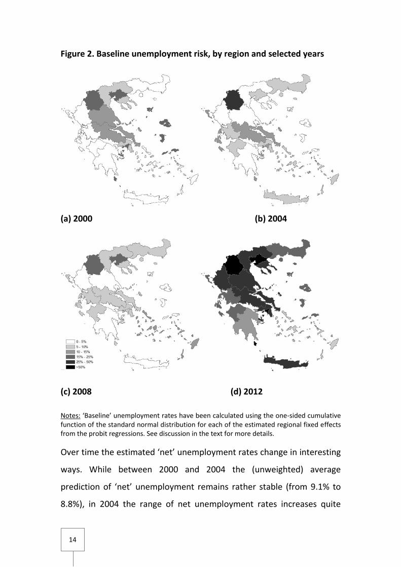
Figure 2. Baseline unemployment risk, by region and selected years

(a) 2000 (b) 2004

(c) 2008 (d) 2012

Notes: ‘Baseline’ unemployment rates have been calculated using the one-sided cumulative function of the standard normal distribution for each of the estimated regional fixed effects from the probit regressions. See discussion in the text for more details.

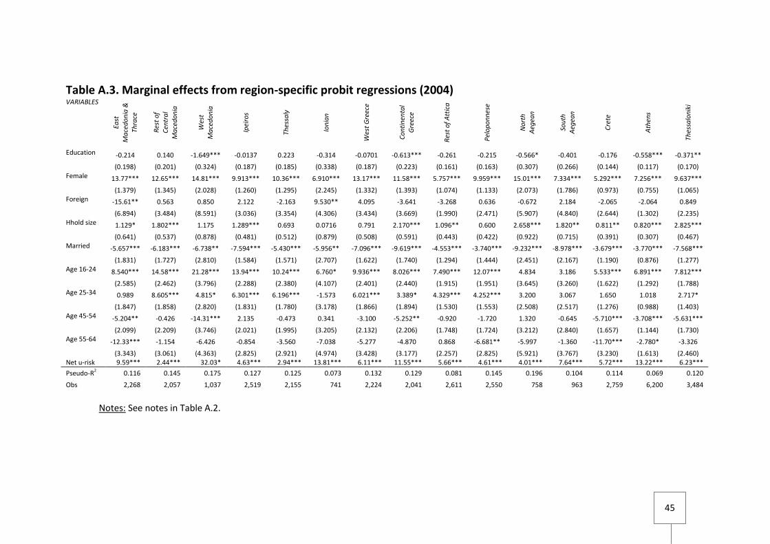
Over time the estimated ‘net’ unemployment rates change in interesting

ways. While between 2000 and 2004 the (unweighted) average

prediction of ‘net’ unemployment remains rather stable (from 9.1% to

8.8%), in 2004 the range of net unemployment rates increases quite

15

15

substantially, with a minimum of 2.4% observed in Central Macedonia

(and similar values in Thessaly, the Peloponnese and the North Aegean)

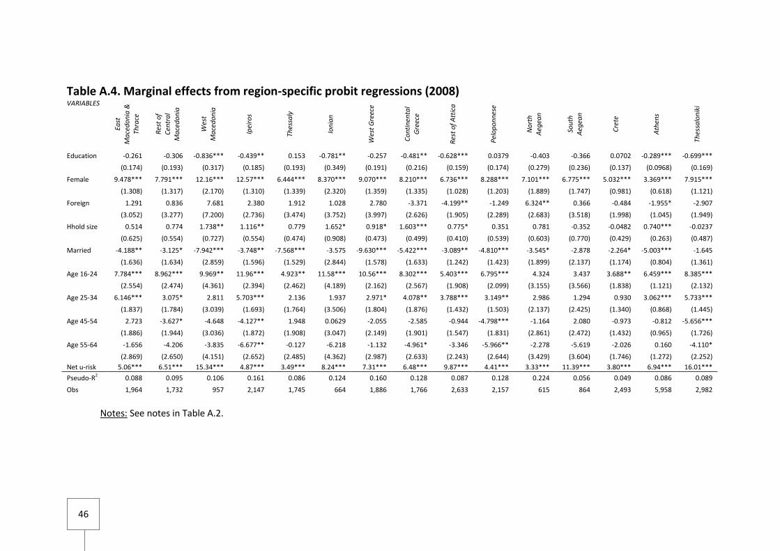
and a maximum, again in Western Macedonia, of 32.0%. By 2008,

average ‘net’ unemployment had declined notably (to 7.5%, roughly

equal to the actual national unemployment rate at the time) and so did

its range (from 3.3% in the North Aegean to 16.0% in Thessaloniki). As

we move into the crisis, however, predicted ‘net’ unemployment rates

rise dramatically (in line with the actual rates), reaching in 2012 an

average value of 31.5%.17 In that year, only one region had a net

unemployment rate below 10% (South Aegean: 6.2%), while values

above 50% were observed in Western Macedonia and the two

metropolitan regions (the maximum was in Thessaloniki at 64.9%).

Clearly, the crisis has represented a significant shock to the Greek labour

market, with net unemployment quadrupling in the space of four years.

Still, the effect across space was very heterogeneous, hitting

disproportionately the north-western and metropolitan regions (and

their hinterlands) but having a much lower impact in the southern and

island regions of the country (fourth panel of Figure 2).

As already noted, the estimated ‘net’ unemployment rates are often

significantly, but far from uniformly, different from the actual

unemployment rates observed in the regions. This suggests that

differences in the mix of workforce characteristics, and especially in the

unemployment risk assigned to each of these, play an important role for

the level of unemployment attained in each region. Thus, our focus now

turns to this latter source of differentiation.

17

Actual national unemployment in spring 2012 was 24.2%.

16

3.2 Unemployment risk and education

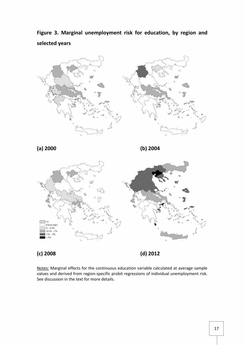
Starting with the education variable (Figure 3), an interesting

observation emerges immediately: for a number of regions, higher levels

of education do not appear to be associated with lower levels of

unemployment risk. This is true throughout the pre-crisis period for the

regions of Eastern Macedonia & Thrace (EMT), Central Macedonia, and

Crete; while for the majority of the remaining regions it is true at least

for subsets of this period. In fact, education returns a statistically

significant negative effect (reducing unemployment) consistently only in

the two metropolitan regions (Athens and Thessaloniki) and the two

partly-industrialised regions of Western Macedonia (energy sector) and

Continental Greece (hosting a part of the Athens industrial complex).

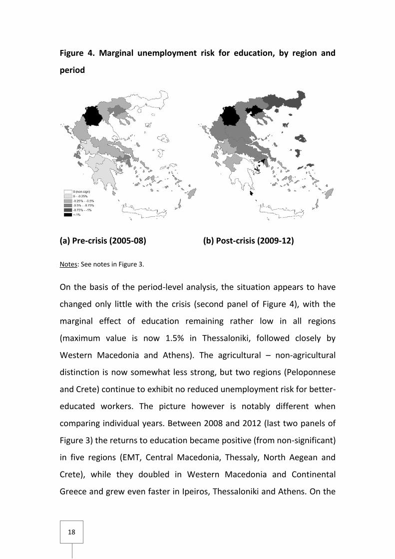
Grouping, however, over the four years preceding the crisis (first panel

of Figure 4), produces results with higher statistical significance. In this

case, education continues to have no effect on unemployment risk in

only four regions (EMT, Thessaly, North Aegean and Crete). The effect is

highest in Western Macedonia (where an additional year of schooling is

associated with a 1.24% drop in the probability of being unemployed).

For most other regions the impact of education is much more modest

(between 0.4% and 0.7%), while it is lowest in the more agricultural

regions of Western Greece and Peloponnese. It appears that prior to the

crisis there was a clear dichotomy between agricultural and non-

agricultural regions in the role that education played in mediating

unemployment risk: in agricultural regions demand for skilled (in terms

of education) labour has been weak – the corollary of this is that these

regions have a relative over-supply of education.

17

17

Figure 3. Marginal unemployment risk for education, by region and

selected years

(a) 2000 (b) 2004

(c) 2008 (d) 2012

Notes: Marginal effects for the continuous education variable calculated at average sample values and derived from region-specific probit regressions of individual unemployment risk. See discussion in the text for more details.

18

Figure 4. Marginal unemployment risk for education, by region and

period

(a) Pre-crisis (2005-08) (b) Post-crisis (2009-12)

Notes: See notes in Figure 3.

On the basis of the period-level analysis, the situation appears to have

changed only little with the crisis (second panel of Figure 4), with the

marginal effect of education remaining rather low in all regions

(maximum value is now 1.5% in Thessaloniki, followed closely by

Western Macedonia and Athens). The agricultural – non-agricultural

distinction is now somewhat less strong, but two regions (Peloponnese

and Crete) continue to exhibit no reduced unemployment risk for better-

educated workers. The picture however is notably different when

comparing individual years. Between 2008 and 2012 (last two panels of

Figure 3) the returns to education became positive (from non-significant)

in five regions (EMT, Central Macedonia, Thessaly, North Aegean and

Crete), while they doubled in Western Macedonia and Continental

Greece and grew even faster in Ipeiros, Thessaloniki and Athens. On the

19

19

other hand, the unemployment risk associated to education increased in

Attica and the Ionian, while it remained non-significant in the

Peloponnese, Western Greece and the South Aegean.

Given the distinctive role of education as an indicator of skills (and as a

screening device for employers), these developments can be used to

make inferences about the functioning of the Greek labour market prior

and during the crisis. Evidently, large parts of Greece are characterised

by an over-supply of skills (over-education). Especially prior to the crisis,

this was also reflected in the above-average unemployment rates for

university graduates (Livanos, 2010b). The crisis is unlikely to have raised

in any significant degree the skill-content of new jobs; but it has created

conditions of job-competition and bumping down, leading to lower

unemployment risks associated with education in large parts of the

country. Still, a number of regions, some of which are at least partly

exposed to international demand (e.g., Attica and the touristic region of

South Aegean), exhibit even today a curious absence of penalties for

lower education. In any case, returns to education (in terms of

employment probabilities) in the country, perhaps with the exception of

Athens and Thessaloniki, remain even today rather low. In one way or

another, these results indicate an overall deficiency in the creation of

skilled jobs in the country and possibly also a qualitative mismatch

between skills supplied and demanded – suggesting problems of labour

market efficiency, at least outside the main urban agglomerations of the

country.

20

3.3 Unemployment risk for other characteristics

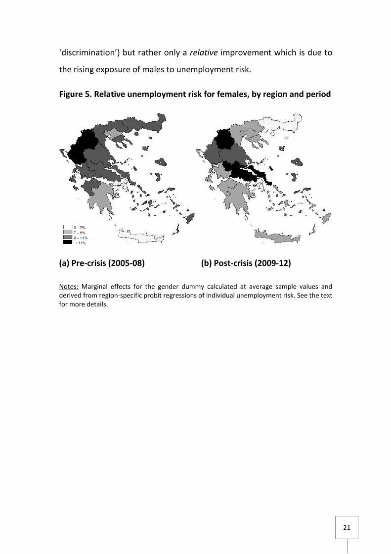
Considerations of labour market efficiency can also be made with regard

to gender and ethnicity, two variables that are often associated with the

presence of labour market discrimination. In the period 2005-2008, the

female penalty (in terms of unemployment risk) ranged between 5.1% in

Athens and 12.6% in Western Macedonia (Figure 5). Most of the regions,

however, had female unemployment risk coefficients (marginal effects)

upwards of 8.5%, consistent with the historical pattern of higher rates of

female unemployment in Greece. Although this may possibly be due to a

greater availability of ‘male’ jobs in (parts of) the country, it is likely also

an indication of some degree of gender discrimination in the labour

market.18 The effect of the crisis is somewhat difficult to distil from the

obtained results. On the one hand, for almost all regions the coefficients

obtained from the probit regressions (not shown) have declined

substantially, indicating an improvement in the relative position of

females during the crisis. On the other hand, the marginal effects

calculated for the gender dummy at average sample values (Table A.2)

show a mixed picture, with relative unemployment risk rising in the

majority of regions (especially Thessaly, Continental Greece and Crete)

and only declining in a few (EMT, Ipeiros, Western Greece and Athens).

The difference between the two sets of results is clearly attributable to

the compositional changes in workforce characteristics that have

occurred between the two periods. Combining the two sets of results, it

is perhaps safe to conclude that the crisis has not brought about an

absolute improvement in the labour market position of females (a fall in 18

Analyses of the female wage penalty in Greece have shown that this is quite substantial, especially

outside the public sector, and indeed can be associated to labour market discrimination, as a large part

of it survives even after controlling for other personal and job characteristics (Kanellopoulos and

Mavromatas, 2002; Livanos and Pouliakas, 2009; Christopoulou and Monastiriotis, 2013).

21

21

‘discrimination’) but rather only a relative improvement which is due to

the rising exposure of males to unemployment risk.

Figure 5. Relative unemployment risk for females, by region and period

(a) Pre-crisis (2005-08) (b) Post-crisis (2009-12)

Notes: Marginal effects for the gender dummy calculated at average sample values and derived from region-specific probit regressions of individual unemployment risk. See the text for more details.

22

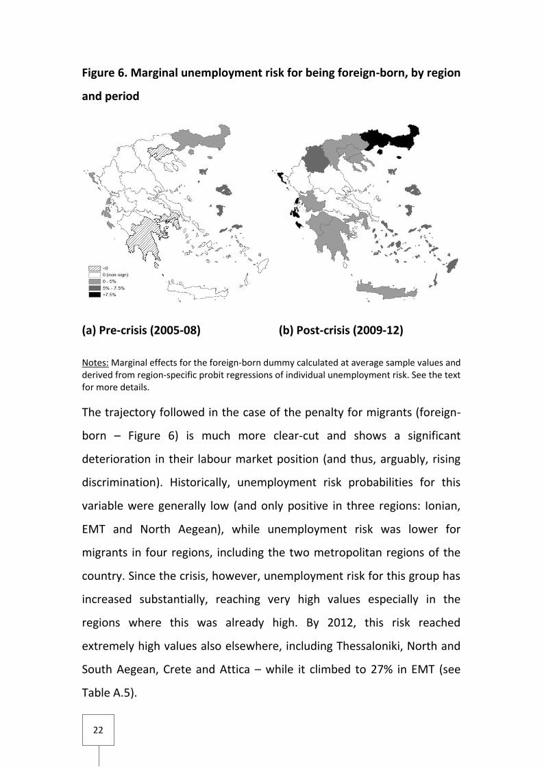
Figure 6. Marginal unemployment risk for being foreign-born, by region

and period

(a) Pre-crisis (2005-08) (b) Post-crisis (2009-12)

Notes: Marginal effects for the foreign-born dummy calculated at average sample values and derived from region-specific probit regressions of individual unemployment risk. See the text for more details.

The trajectory followed in the case of the penalty for migrants (foreign-

born – Figure 6) is much more clear-cut and shows a significant

deterioration in their labour market position (and thus, arguably, rising

discrimination). Historically, unemployment risk probabilities for this

variable were generally low (and only positive in three regions: Ionian,

EMT and North Aegean), while unemployment risk was lower for

migrants in four regions, including the two metropolitan regions of the

country. Since the crisis, however, unemployment risk for this group has

increased substantially, reaching very high values especially in the

regions where this was already high. By 2012, this risk reached

extremely high values also elsewhere, including Thessaloniki, North and

South Aegean, Crete and Attica – while it climbed to 27% in EMT (see

Table A.5).

23

23

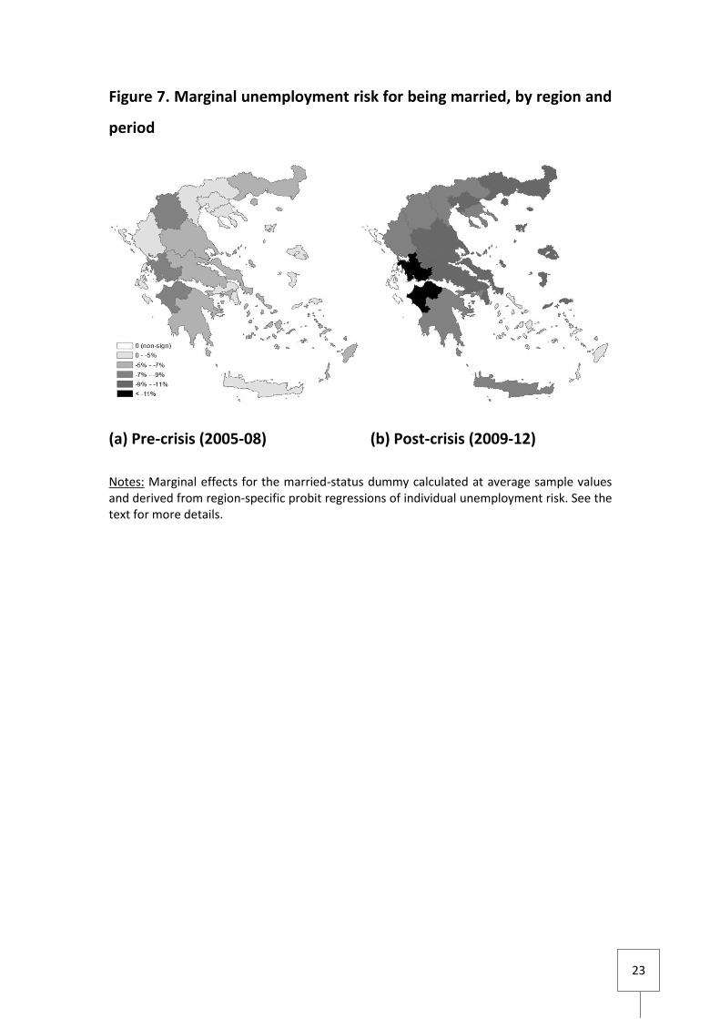
Figure 7. Marginal unemployment risk for being married, by region and

period

(a) Pre-crisis (2005-08) (b) Post-crisis (2009-12)

Notes: Marginal effects for the married-status dummy calculated at average sample values and derived from region-specific probit regressions of individual unemployment risk. See the text for more details.

24

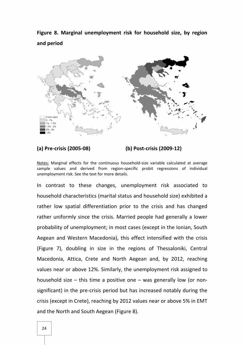
Figure 8. Marginal unemployment risk for household size, by region

and period

(a) Pre-crisis (2005-08) (b) Post-crisis (2009-12)

Notes: Marginal effects for the continuous household-size variable calculated at average sample values and derived from region-specific probit regressions of individual unemployment risk. See the text for more details.

In contrast to these changes, unemployment risk associated to

household characteristics (marital status and household size) exhibited a

rather low spatial differentiation prior to the crisis and has changed

rather uniformly since the crisis. Married people had generally a lower

probability of unemployment; in most cases (except in the Ionian, South

Aegean and Western Macedonia), this effect intensified with the crisis

(Figure 7), doubling in size in the regions of Thessaloniki, Central

Macedonia, Attica, Crete and North Aegean and, by 2012, reaching

values near or above 12%. Similarly, the unemployment risk assigned to

household size – this time a positive one – was generally low (or non-

significant) in the pre-crisis period but has increased notably during the

crisis (except in Crete), reaching by 2012 values near or above 5% in EMT

and the North and South Aegean (Figure 8).

25

25

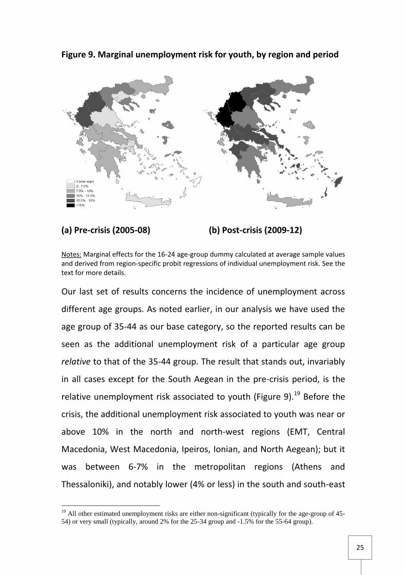
Figure 9. Marginal unemployment risk for youth, by region and period

(a) Pre-crisis (2005-08) (b) Post-crisis (2009-12)

Notes: Marginal effects for the 16-24 age-group dummy calculated at average sample values and derived from region-specific probit regressions of individual unemployment risk. See the text for more details.

Our last set of results concerns the incidence of unemployment across

different age groups. As noted earlier, in our analysis we have used the

age group of 35-44 as our base category, so the reported results can be

seen as the additional unemployment risk of a particular age group

relative to that of the 35-44 group. The result that stands out, invariably

in all cases except for the South Aegean in the pre-crisis period, is the

relative unemployment risk associated to youth (Figure 9).19 Before the

crisis, the additional unemployment risk associated to youth was near or

above 10% in the north and north-west regions (EMT, Central

Macedonia, West Macedonia, Ipeiros, Ionian, and North Aegean); but it

was between 6-7% in the metropolitan regions (Athens and

Thessaloniki), and notably lower (4% or less) in the south and south-east

19

All other estimated unemployment risks are either non-significant (typically for the age-group of 45-

54) or very small (typically, around 2% for the 25-34 group and -1.5% for the 55-64 group).

26

regions (Attica, South Aegean and Crete). This geographical distribution

changed quite sizeably during the crisis: parts of the north (West

Macedonia, Ipeiros and Central Macedonia) continued to be on the top

of the distribution, but other parts of this group (Ionian and North

Aegean) have now amongst the lowest youth penalties (together with

Crete). The South Aegean and Attica, which in the past carried small or

no youth penalties, have now a penalty of over 12%, and group together

with Continental Greece and Thessaloniki, which also saw sizeable

increases in this penalty. In contrast, Athens, EMT and the Peloponnese

only saw rather modest increases. Overall, between the two periods the

relative unemployment risk for the 15-24 age-group rose by over 50%. It

should be noted, however, that – as with the case of the female penalty

– this effect is almost entirely compositional, as the direct probit

estimates (z-scores) present a rather different picture, with the youth

unemployment penalty being in the vast majority of cases not

significantly different, in a statistical sense, between the two periods.

Changes in the relative unemployment risk for other age groups are

much more modest (typically less than 20% and often negative or non-

significant) – with the exception perhaps of West Macedonia and

Continental Greece, where the unemployment risk for older age groups

(relative to the 35-44 group) declined rather substantially, and the

regions of Thessaly, Thessaloniki and Western Greece, where the

relative unemployment risk for the 24-35 group increased quite sizeably

(see Tables A2-A5 in Appendix).

27

27

4. Decomposition analysis: macro-geographies of

unemployment

The analysis undertaken thus far has revealed a at times substantial

degree of regional differentiation both in terms of the unemployment

risk assigned to individual characteristics and in terms of changes in this

risk during the crisis. Moreover, it has revealed that compositional

changes (or differences between regions) may be playing an important

role in determining the size of the imputed unemployment risk (marginal

effects) for different characteristics. To disentangle the effect of such

compositional movements/differences from that of pure valuation

changes, we proceed in this section to a decomposition analysis as

explained in section 2. We do not implement this decomposition for

each region separately but rather apply our analysis on a number of

regional groupings that we construct. This is partly for ease of

presentation, but also serves the additional purpose of allowing us to

explore the spatial variation in the incidence and the determinants of

unemployment risk along wider geographical lines and divisions (macro-

geographies) – and to link these to possible structural or systemic factors

that may be responsible for the observed variation.

Among the possible factors of differentiation, we look in this paper at

factors that have to do with differences in production structures

(agricultural versus non-agricultural regions), agglomeration (Athens, as

the only significant financial and economic centre in the country, versus

the rest of Greece), physical geography (island versus mainland regions),

historical-political geography (north versus south), and labour market

performance (high- versus low-unemployment regions). Membership of

regions to these groups is presented in the Appendix. We base our

28

analysis on the Neumark (pooled-estimate) decomposition, which

expresses the ‘endowments’ component in terms of average (full-

sample) coefficients.20 Consistent with our earlier discussion, which

separated between three types of effects (effective demand, labour

quality and valuation of endowments), we present two sets of results for

each decomposition. The standard decomposition is presented by means

of graphs; while the decomposition splitting further the ‘coefficients’

component into ‘valuation’ and ‘effective demand’ is presented in

summary form (selected years) in a table. As will become clear later, this

is because splitting the standard ‘coefficients’ component into these two

sub-components produces large differences that are difficult to present

graphically.21

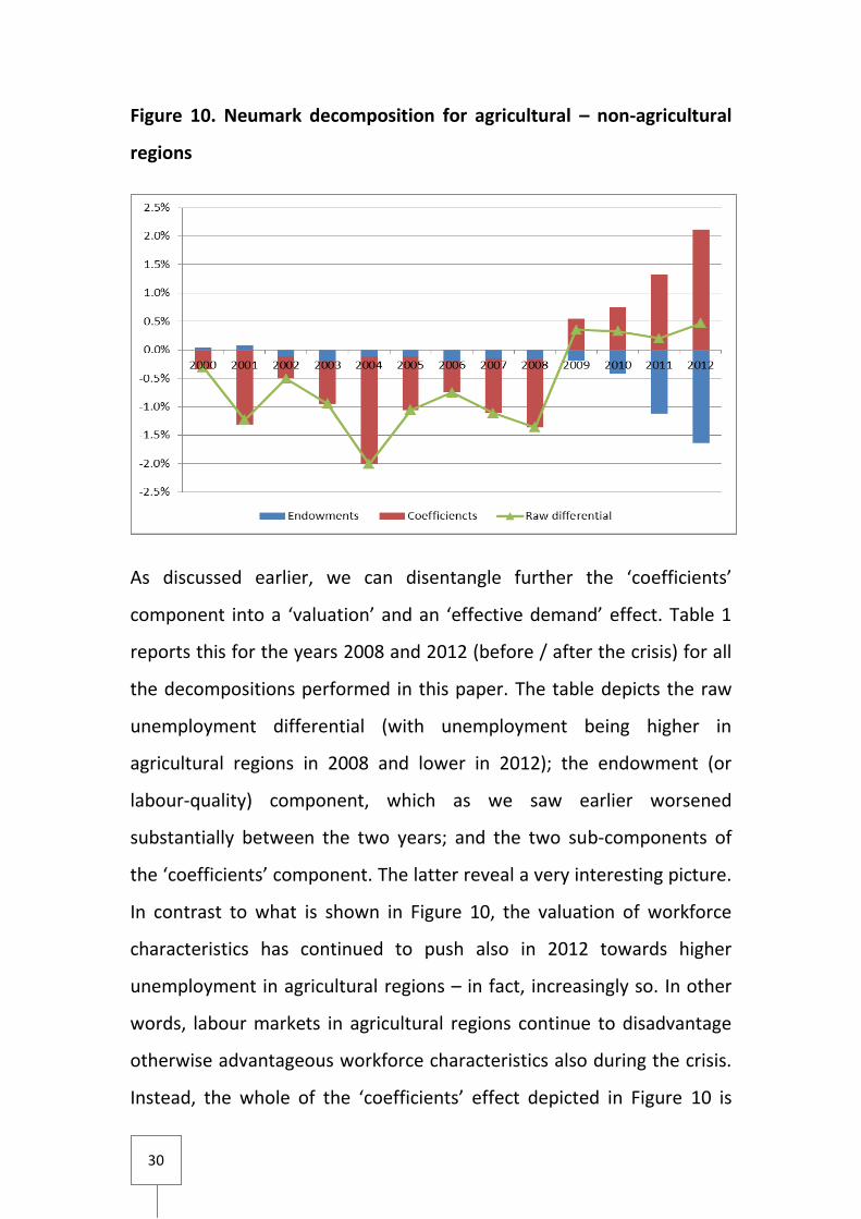
We start our discussion here with a decomposition on the basis of

production structures (agriculture).22 Figure 10 reveals an interesting

picture of a decade-long difference that has been substantially altered

by the crisis. Until 2008, unemployment in agricultural regions oscillated

between half and two percentage points above the rate found in non-

agricultural regions. By far, the biggest part of this differential was due

to this group’s inferior performance with regard to the valuation of

workforce characteristics (‘coefficients’ component). In other words,

most of the higher unemployment in these regions in the 2000-2008

period is attributable to the relative inability of their labour markets to

channel into employment individuals possessing characteristics that in

20

Results using other decomposition methods produce qualitatively similar conclusions and are

available upon request. 21

Lopez-Bazo and Montellon (2013), in their regional decomposition of unemployment risk (for the

case of Spain), also find substantial differences within the ‘coefficients’ component. 22

Recall from section 2 that specialisation in agriculture appeared as a potentially relevant factor of

differentiation in the case of education, with more agricultural regions having lower unemployment

risks associated to education, especially prior to the crisis.

29

29

non-agricultural regions were typically producing less unemployment.23

The situation seems to have been reversed with the crisis. As early as in

2009, and increasingly over time, the ‘coefficients’ component becomes

positive, suggesting that the valuation of workforce characteristics is

now more advantageous in agricultural regions – which now have

below-average unemployment rates (albeit marginally so). The

‘endowments’ component moves in the opposite direction, becoming

more and more negative, indicating in turn that non-agricultural regions

obtain an increasing relative advantage in terms of workforce skills.

Without this, the unemployment differential would have been

significantly higher – by over 1.5 percentage points in 2012 (four times

higher). This is an extremely interesting observation, especially in

relation to common perceptions about an ‘exodus’ of talented workers

to the countryside.24

23

In fact, when valuated at coefficients obtained for the non-agricultural group (standard Blinder-

Oaxaca decomposition), the ‘endowments’ component is positive, suggesting that agricultural regions

had higher concentration of workforce characteristics that were more ‘marketable’ in the non-

agricultural regions. 24

See for example the Guardian, 13/5/2011

(available at http://www.guardian.co.uk/world/2011/may/13/greek-crisis-athens-rural-migration).

30

Figure 10. Neumark decomposition for agricultural – non-agricultural

regions

As discussed earlier, we can disentangle further the ‘coefficients’

component into a ‘valuation’ and an ‘effective demand’ effect. Table 1

reports this for the years 2008 and 2012 (before / after the crisis) for all

the decompositions performed in this paper. The table depicts the raw

unemployment differential (with unemployment being higher in

agricultural regions in 2008 and lower in 2012); the endowment (or

labour-quality) component, which as we saw earlier worsened

substantially between the two years; and the two sub-components of

the ‘coefficients’ component. The latter reveal a very interesting picture.

In contrast to what is shown in Figure 10, the valuation of workforce

characteristics has continued to push also in 2012 towards higher

unemployment in agricultural regions – in fact, increasingly so. In other

words, labour markets in agricultural regions continue to disadvantage

otherwise advantageous workforce characteristics also during the crisis.

Instead, the whole of the ‘coefficients’ effect depicted in Figure 10 is

31

31

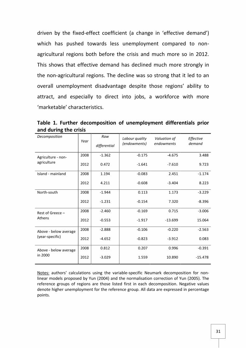
driven by the fixed-effect coefficient (a change in ‘effective demand’)

which has pushed towards less unemployment compared to non-

agricultural regions both before the crisis and much more so in 2012.

This shows that effective demand has declined much more strongly in

the non-agricultural regions. The decline was so strong that it led to an

overall unemployment disadvantage despite those regions’ ability to

attract, and especially to direct into jobs, a workforce with more

‘marketable’ characteristics.

Table 1. Further decomposition of unemployment differentials prior and during the crisis Decomposition

Year Raw

differential

Labour quality (endowments)

Valuation of endowments

Effective demand

Agriculture - non-agriculture

2008 -1.362 -0.175 -4.675 3.488

2012 0.472 -1.641 -7.610 9.723

Island - mainland 2008 1.194 -0.083 2.451 -1.174

2012 4.211 -0.608 -3.404 8.223

North-south 2008 -1.944 0.113 1.173 -3.229

2012 -1.231 -0.154 7.320 -8.396

Rest of Greece – Athens

2008 -2.460 -0.169 0.715 -3.006

2012 -0.553 -1.917 -13.699 15.064

Above - below average (year-specific)

2008 -2.888 -0.106 -0.220 -2.563

2012 -4.652 -0.823 -3.912 0.083

Above - below average in 2000

2008 0.812 0.207 0.996 -0.391

2012 -3.029 1.559 10.890 -15.478

Notes: authors’ calculations using the variable-specific Neumark decomposition for non-linear models proposed by Yun (2004) and the normalisation correction of Yun (2005). The reference groups of regions are those listed first in each decomposition. Negative values denote higher unemployment for the reference group. All data are expressed in percentage points.

32

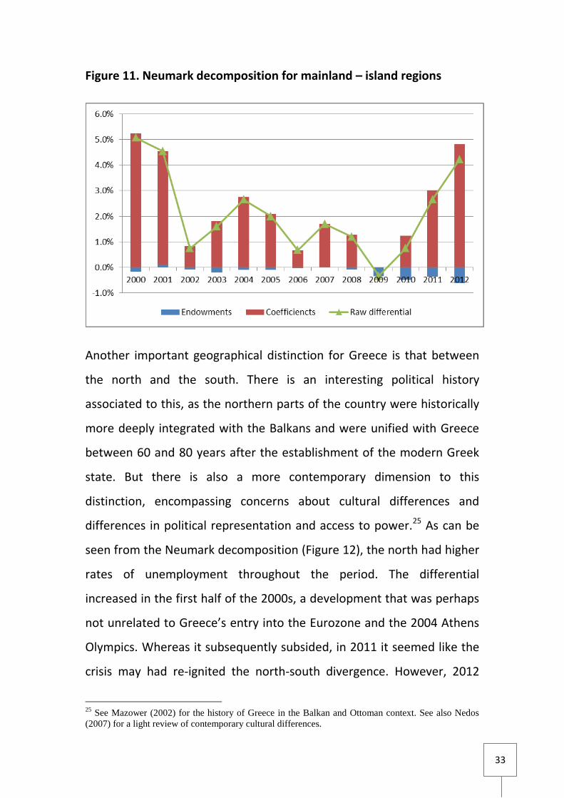
The role of effective demand is important also along other dimensions.

Turning to the island – mainland distinction (Figure 11), we first note

that unemployment differentials between these two groups have been

rather volatile over the years, but were particularly high (near 5%) in the

beginning and the end of the period, rising sharply during the crisis. The

differential has throughout the period been driven by the ‘coefficients’

component, as the endowments component is by comparison very low.

In 2008, much of the differential was accounted for by a more

advantageous valuation of endowments, as effective demand was lower

than in mainland Greece (Table 1). In contrast, in 2012 the effective

demand component became hugely important in giving an

unemployment advantage to the island regions, as apparently effective

demand collapsed much more strongly in mainland Greece. According to

the ‘valuation’ component, mainland regions responded to this fall in

demand by improving the way in which they reward (in terms of

employment probabilities) the characteristics of their workforce: this

helped contain the sizeable fall in relative demand, producing a raw

unemployment differential which is almost half the ‘effective demand’

differential (4.2 and 8.2, respectively).

33

33

Figure 11. Neumark decomposition for mainland – island regions

Another important geographical distinction for Greece is that between

the north and the south. There is an interesting political history

associated to this, as the northern parts of the country were historically

more deeply integrated with the Balkans and were unified with Greece

between 60 and 80 years after the establishment of the modern Greek

state. But there is also a more contemporary dimension to this

distinction, encompassing concerns about cultural differences and

differences in political representation and access to power.25 As can be

seen from the Neumark decomposition (Figure 12), the north had higher

rates of unemployment throughout the period. The differential

increased in the first half of the 2000s, a development that was perhaps

not unrelated to Greece’s entry into the Eurozone and the 2004 Athens

Olympics. Whereas it subsequently subsided, in 2011 it seemed like the

crisis may had re-ignited the north-south divergence. However, 2012

25

See Mazower (2002) for the history of Greece in the Balkan and Ottoman context. See also Nedos

(2007) for a light review of contemporary cultural differences.

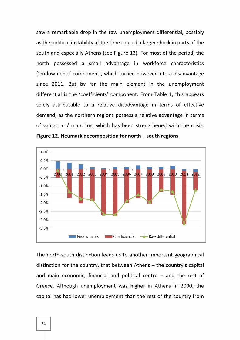
34

saw a remarkable drop in the raw unemployment differential, possibly

as the political instability at the time caused a larger shock in parts of the

south and especially Athens (see Figure 13). For most of the period, the

north possessed a small advantage in workforce characteristics

(‘endowments’ component), which turned however into a disadvantage

since 2011. But by far the main element in the unemployment

differential is the ‘coefficients’ component. From Table 1, this appears

solely attributable to a relative disadvantage in terms of effective

demand, as the northern regions possess a relative advantage in terms

of valuation / matching, which has been strengthened with the crisis.

Figure 12. Neumark decomposition for north – south regions

The north-south distinction leads us to another important geographical

distinction for the country, that between Athens – the country’s capital

and main economic, financial and political centre – and the rest of

Greece. Although unemployment was higher in Athens in 2000, the

capital has had lower unemployment than the rest of the country from

35

35

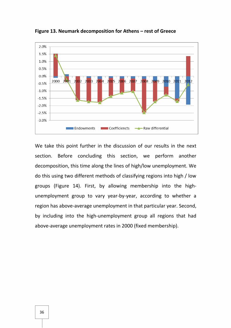
2001 onwards (Figure 13).26 The decline of relative unemployment for

the capital in the early period appears to have been due to a relative

improvement in the ‘coefficients’ component, which remained

advantageous until recently but by 2012 had turned into a disadvantage

(with a sizeable decline during the crisis). Instead, the ‘endowments’

component started becoming more advantageous for Athens with the

crisis, pushing unemployment downwards (relative to the rest of the

country) by almost 2 percentage points by 2012. But the main factor

containing unemployment in Athens during the crisis appears to have

been the capital’s ability to adjust to the huge demand shock instigated

by the crisis: according to the decomposition of Table 1, between 2008

and 2012 Athens experienced a fall in effective demand, relative to the

rest of the country, of over 15 percentage points; the containment of the

unemployment differential to just over half a percentage point by 2012

was for the largest part attributed to a huge rise in the capital’s

‘valuation’ advantage, showing a far better ability to mobilise

‘marketable’ workforce characteristics relative to the rest of the country.

This finding seems to compromise two rather antithetical views about

the geography of the crisis in Greece: on the one hand, the common

perception that the crisis hit hardest the capital; on the other hand, that

unemployment has reached exceptionally high levels more outside

Athens than in the capital.

26

An interesting observation with regard to Athens is the significant decline in relative unemployment

in 2008, the year immediately before the crisis, when Greece – quite ironically – achieved its lower

unemployment rate for almost two decades. On the basis of Figure 13, it appears that the achievement

of this historical low was in large part driven by the performance of the capital’s labour market.

36

Figure 13. Neumark decomposition for Athens – rest of Greece

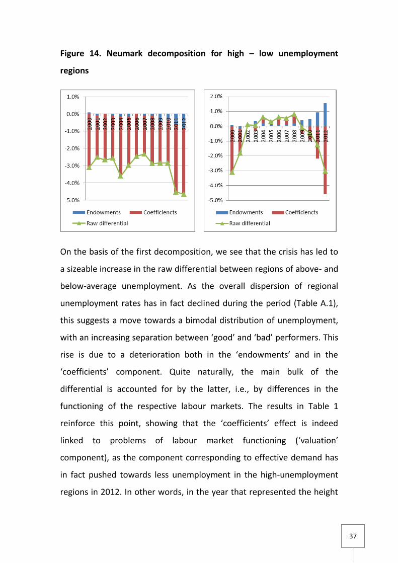
We take this point further in the discussion of our results in the next

section. Before concluding this section, we perform another

decomposition, this time along the lines of high/low unemployment. We

do this using two different methods of classifying regions into high / low

groups (Figure 14). First, by allowing membership into the high-

unemployment group to vary year-by-year, according to whether a

region has above-average unemployment in that particular year. Second,

by including into the high-unemployment group all regions that had

above-average unemployment rates in 2000 (fixed membership).

37

37

Figure 14. Neumark decomposition for high – low unemployment

regions

On the basis of the first decomposition, we see that the crisis has led to

a sizeable increase in the raw differential between regions of above- and

below-average unemployment. As the overall dispersion of regional

unemployment rates has in fact declined during the period (Table A.1),

this suggests a move towards a bimodal distribution of unemployment,

with an increasing separation between ‘good’ and ‘bad’ performers. This

rise is due to a deterioration both in the ‘endowments’ and in the

‘coefficients’ component. Quite naturally, the main bulk of the

differential is accounted for by the latter, i.e., by differences in the

functioning of the respective labour markets. The results in Table 1

reinforce this point, showing that the ‘coefficients’ effect is indeed

linked to problems of labour market functioning (‘valuation’

component), as the component corresponding to effective demand has

in fact pushed towards less unemployment in the high-unemployment

regions in 2012. In other words, in the year that represented the height

38

of the crisis, high-unemployment regions were not those that

experienced a deeper demand shock but rather those that failed to

sufficiently ‘reward’ available and otherwise marketable workforce

characteristics.

The fixed-membership decomposition (second panel of Figure 14) offers

another interesting observation. As can be seen, the regions suffering

most today were performing, as a group, above the national average for

most of the period prior to the crisis; but they had a significantly worse

unemployment performance in the first years of the century (and

possibly also in the 1990s). This is consistent with the view that the crisis

has affected most those regions that had benefited more from the boom

years after Greece’s entry into the Eurozone. Interestingly, in both 2008

and 2012, these regions had better workforce characteristics and better

valuation of those characteristics (Table 1) – they had in other words

better-functioning labour markets and a more ‘marketable’ workforce.

However, already in 2008 and much more emphatically in 2012, they

had substantially lower effective demand relative to the rest of the

country. This reaffirms the interpretation of these regions as the regions

on the top of the boom-and-bust cycle.

5. Conclusions

The crisis has led to an unprecedented increase in unemployment in

Greece, raising concerns about economic sustainability and social

cohesion in the country. Given the huge shock nationally and perhaps

the political and economic centrality of Athens, attention to the spatial

dimension of the crisis has been subdued. This is reinforced by the fact

39

39

that, at the aggregate level, spatial patterns of unemployment and

unemployment evolutions are rather mixed and difficult to describe

using macro-geographical distinctions.

In this paper we moved beyond the descriptive diagnosis of ‘rising

unemployment’ and, making use of recent advances in decomposition

techniques, we examined the dynamics of unemployment and labour

market adjustment in the Greek regions using micro-data from the

Greek LFS. We identified, and were able to measure, three distinctive

influences on the regional labour markets, corresponding to

differences/changes in labour quality, matching efficiency (valuation)

and effective demand. Differences in effective demand, especially during

the crisis, were found to be large, with the demand shock hitting

disproportionately the metropolitan and north/north-western regions.

Adjustment in terms of valuation of workforce characteristics (matching

efficiency) was also heterogeneous, being stronger in the mainland non-

agricultural regions and especially in Athens. Crucially, the high-

unemployment regions during the crisis are not those that suffered the

largest demand shock (as measured by the rise in ‘baseline’

unemployment risk) but rather those that displayed a relative

disadvantage in matching efficiency (and, less so, in labour quality).

Overall, problems of matching efficiency / valuation have been found to

be an important part of the unemployment story in Greece. Especially in

relation to education, our results suggest an important deficiency in the

Greek labour market(s), as employment probabilities associated to

education (years of schooling) appear particularly low (often not

different from zero) and have increased only slightly during the crisis. A

number of important conclusions can be derived from this.

40

First, high-unemployment regions – and perhaps the country as a whole

– suffer from a relative over-education problem, meaning that education

is over-supplied relative to the demand for skills and thus not sufficiently

rewarded. In turn, this suggests two things. On the one hand, that the

skill-content of jobs in Greece (both before and during the crisis) is

rather low, showing a deficiency in the availability of ‘good’, high-

productivity jobs. On the other hand, that the education system in

Greece produces skills that are not directly marketable in the Greek

labour market, showing a qualitative mismatch between skills demanded

and skills produced.

Second, the extent of job-competition in the country is rather limited.

Across space, both before and during the crisis, slack labour markets

have been found to have low (or zero) penalties for unfavourable

workforce characteristics. Unemployment risk coefficients have

increased (in absolute terms) with the crisis, but compared to the size of

the shock and the extent of depression of the economy, the increase is

not particularly sizeable – suggesting that job-competition and bumping-

down have intensified only to a limited extent. Although for some

exogenous characteristics (gender, ethnicity) this may not be seen as a

problem (especially as it may also be taken to imply low levels of labour

market discrimination), for acquired characteristics (especially

education) it rather signals a malfunctioning of the labour market,

indicating that incentives for the accumulation of advantageous

workforce characteristics – and the rewards for these – are also low.

Last but not least, intra-and inter-regional adjustment mechanisms in

the country – perhaps with very few exceptions, mainly in the

41

41

metropolitan areas – appear also particularly weak. As Figures 10-14

show, valuation differentials are sizeable and rather persistent;

especially in the period before the crisis, they have been the main

component accounting for unemployment differences across space. It

follows that the responsiveness of labour supply (including through

migration) to differences in unemployment risk is very low. This is most

probably not unrelated to the various institutional rigidities in the

country (including in the labour and housing markets), but it also reflects

perhaps a more attitudinal source of rigidity that has to do with people’s

preferences (e.g., about locality) and the informal institutions associated

to these (e.g., social networks, role of extended family, etc).

These observations have an important policy dimension. Identifying and

understanding the specific conditions shaping unemployment risk at the

individual and regional levels can help inform the design of relevant

policies, including place-based ones, that will respond to the specific

circumstances of each local labour market and its workforce. This is

especially important for the depressed economy of Greece, where a

demand-led exit from unemployment is quite unlikely. As an example,

knowing that education does not ‘pay’ (in terms of employment

probabilities) in regions such as Crete and the Peloponnese can direct

policy – especially in the contemporary context of continuing austerity

and private-sector disinvestment – towards actions that selectively

attempt to diversify the skills of the better-educated in those regions or

to increase their mobility (while pursuing in the longer-run a strategy to

increase the demand for skills in these labour markets). Instead, knowing

that education carries a very high premium in the regions of Thessaloniki

and Western Macedonia ought to direct policy towards measures that

42

seek to raise the educational qualifications – or the related labour

market skills – of the local workforce and/or to attract educated workers

into these regions. In a time of crisis and overall demand deficiency,

finding the appropriate policy measures to tackle unemployment and,

moreover, fine-tuning them across space and in response to specific

labour market conditions is – needless to say – of paramount

importance, not only in economic terms but also on social grounds. We

believe that the range and character of the results unveiled in this paper

make a small, but highly relevant contribution to this.

43

43

APPENDIX

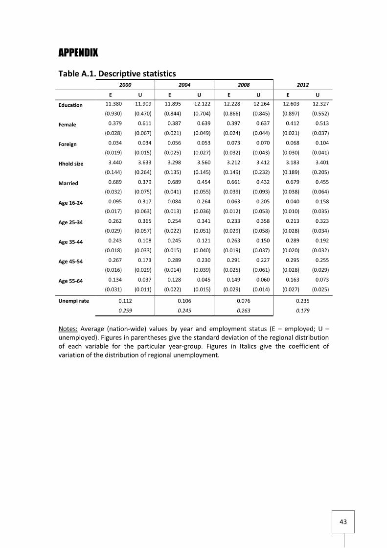
Table A.1. Descriptive statistics 2000 2004 2008 2012

E U E U E U E U

Education 11.380 11.909 11.895 12.122 12.228 12.264 12.603 12.327

(0.930) (0.470) (0.844) (0.704) (0.866) (0.845) (0.897) (0.552)

Female 0.379 0.611 0.387 0.639 0.397 0.637 0.412 0.513

(0.028) (0.067) (0.021) (0.049) (0.024) (0.044) (0.021) (0.037)

Foreign 0.034 0.034 0.056 0.053 0.073 0.070 0.068 0.104

(0.019) (0.015) (0.025) (0.027) (0.032) (0.043) (0.030) (0.041)

Hhold size 3.440 3.633 3.298 3.560 3.212 3.412 3.183 3.401

(0.144) (0.264) (0.135) (0.145) (0.149) (0.232) (0.189) (0.205)

Married 0.689 0.379 0.689 0.454 0.661 0.432 0.679 0.455

(0.032) (0.075) (0.041) (0.055) (0.039) (0.093) (0.038) (0.064)

Age 16-24 0.095 0.317 0.084 0.264 0.063 0.205 0.040 0.158

(0.017) (0.063) (0.013) (0.036) (0.012) (0.053) (0.010) (0.035)

Age 25-34 0.262 0.365 0.254 0.341 0.233 0.358 0.213 0.323

(0.029) (0.057) (0.022) (0.051) (0.029) (0.058) (0.028) (0.034)

Age 35-44 0.243 0.108 0.245 0.121 0.263 0.150 0.289 0.192

(0.018) (0.033) (0.015) (0.040) (0.019) (0.037) (0.020) (0.032)

Age 45-54 0.267 0.173 0.289 0.230 0.291 0.227 0.295 0.255

(0.016) (0.029) (0.014) (0.039) (0.025) (0.061) (0.028) (0.029)

Age 55-64 0.134 0.037 0.128 0.045 0.149 0.060 0.163 0.073

(0.031) (0.011) (0.022) (0.015) (0.029) (0.014) (0.027) (0.025)

Unempl rate 0.112 0.106 0.076 0.235

0.259 0.245 0.263 0.179

Notes: Average (nation-wide) values by year and employment status (E – employed; U – unemployed). Figures in parentheses give the standard deviation of the regional distribution of each variable for the particular year-group. Figures in Italics give the coefficient of variation of the distribution of regional unemployment.

44

Table A.2. Marginal effects from region-specific probit regressions (2000) VARIABLES

East

Ma

ced

on

ia &

Th

race

Res

t o

f C

entr

al

Ma

ced

on

ia

Wes

t M

ace

do

nia

Ipei

ros

Thes

saly

Ion

ian

Wes

t G

reec

e

Co

nti

nen

tal

Gre

ece

Res

t o

f A

ttic

a

Pel

op

on

nes

e

No

rth

A

egea

n

Sou

th

Aeg

ean

Cre

te

Ath

ens

Thes

salo

nik

i

Education 0.162 0.0833 -0.819** -0.240 -0.451** 0.214 0.324* -0.622*** -0.311 0.178 -0.795*** -0.000718 -0.0162 -0.883*** -0.754***

(0.166) (0.183) (0.330) (0.220) (0.216) (0.245) (0.177) (0.241) (0.206) (0.188) (0.285) (0.262) (0.159) (0.103) (0.162)

Female 5.973*** 11.28*** 10.52*** 10.99*** 16.67*** 2.316 7.862*** 13.69*** 9.290*** 9.989*** 9.205*** 4.944*** 7.575*** 7.953*** 7.717***

(1.197) (1.251) (2.027) (1.525) (1.438) (1.749) (1.282) (1.529) (1.355) (1.307) (1.961) (1.552) (1.182) (0.674) (1.077)

Foreign 9.080** 8.568 11.88 0.000 4.461 2.158 -6.175 -2.785 -10.56*** 3.131 19.38** 1.388 2.895 -0.647 -5.041

(4.115) (5.305) (9.298) (0.000) (5.588) (5.700) (5.170) (6.573) (3.718) (3.772) (9.314) (4.771) (3.010) (1.422) (3.274)

Hhold size 0.554 -0.809 -0.644 1.678** 0.423 1.067 1.419*** 0.940 1.590*** -0.0534 0.645 1.956*** 0.182 1.060*** 0.781

(0.489) (0.512) (0.915) (0.654) (0.553) (0.771) (0.462) (0.604) (0.477) (0.541) (0.752) (0.689) (0.427) (0.287) (0.483)

Married -4.878*** -6.577*** -1.953 -6.468*** -8.231*** -5.215** -8.666*** -4.733** -8.691*** -5.014*** -6.494*** -3.380 -4.981*** -8.224*** -9.953***

(1.556) (1.619) (2.694) (2.109) (1.772) (2.131) (1.567) (2.011) (1.772) (1.737) (2.250) (2.189) (1.429) (0.806) (1.385)

Age 16-24 7.805*** 10.90*** 23.55*** 11.33*** 10.36*** 2.716 12.78*** 18.18*** 6.851*** 11.49*** 3.559 7.675** 7.030*** 11.12*** 8.727***

(2.207) (2.115) (3.715) (2.998) (2.546) (3.081) (2.087) (2.644) (2.364) (2.416) (2.983) (3.134) (1.903) (1.186) (1.907)

Age 25-34 5.568*** 4.588*** 7.623*** 7.208*** 6.646*** 6.050** 5.527*** 7.327*** 0.229 4.164** 3.616 4.629* 1.193 5.918*** 4.207***

(1.768) (1.766) (2.785) (2.344) (2.045) (2.430) (1.803) (2.278) (1.985) (1.893) (2.458) (2.693) (1.639) (0.939) (1.555)

Age 45-54 1.390 -4.670** -5.450 -2.323 -4.547* -2.064 -1.699 -5.155* -3.081 -1.140 -6.510* 1.384 -5.310** -1.287 -0.704

(1.936) (2.202) (3.477) (2.560) (2.549) (3.240) (2.285) (2.690) (2.241) (2.081) (3.911) (3.026) (2.221) (1.107) (1.721)

Age 55-64 -6.388** -9.672*** -10.13** -7.861** -12.83*** -0.312 -4.323 -11.46*** -3.470 -9.379*** -10.98* 2.426 -10.03*** -0.648 -2.384

(3.051) (3.260) (4.837) (3.493) (3.824) (3.905) (3.414) (3.831) (3.095) (3.295) (6.191) (3.849) (3.067) (1.535) (2.717)

Net u-risk 4.35*** 8.77*** 20.07*** 4.87*** 10.10*** 1.37*** 2.25*** 10.08*** 9.91*** 4.99*** 16.43** 0.49*** 4.90*** 18.51*** 19.49***

Pseudo-R2 0.087 0.179 0.130 0.151 0.194 0.128 0.188 0.176 0.118 0.139 0.171 0.135 0.158 0.102 0.112

Obs 2,186 2,201 1,093 1,558 1,869 755 2,191 1,800 2,108 2,006 702 960 2,079 8,956 3,375

Notes: Marginal effects (multiplied by 100 / expressed in percentage points) calculated on average sample values (standard errors in parentheses).

‘Net unemployment risk’ is the cumulative probability (one-sided) of the standard normal distribution associated to the corresponding fixed effect

(see text for details). *, ** and *** show significance at 10%, 5% and 1%, respectively.

45

Table A.3. Marginal effects from region-specific probit regressions (2004) VARIABLES

East

Ma

ced

on

ia &

Th

race

Res

t o

f C

entr

al

Ma

ced

on

ia

Wes

t M

ace

do

nia

Ipei

ros

Thes

saly

Ion

ian

Wes

t G

reec

e

Co

nti

nen

tal

Gre

ece

Res

t o

f A

ttic

a

Pel

op

on

nes

e

No

rth

A

egea

n

Sou

th

Aeg

ean

Cre

te

Ath

ens

Thes

salo

nik

i

Education -0.214 0.140 -1.649*** -0.0137 0.223 -0.314 -0.0701 -0.613*** -0.261 -0.215 -0.566* -0.401 -0.176 -0.558*** -0.371** (0.198) (0.201) (0.324) (0.187) (0.185) (0.338) (0.187) (0.223) (0.161) (0.163) (0.307) (0.266) (0.144) (0.117) (0.170) Female 13.77*** 12.65*** 14.81*** 9.913*** 10.36*** 6.910*** 13.17*** 11.58*** 5.757*** 9.959*** 15.01*** 7.334*** 5.292*** 7.256*** 9.637*** (1.379) (1.345) (2.028) (1.260) (1.295) (2.245) (1.332) (1.393) (1.074) (1.133) (2.073) (1.786) (0.973) (0.755) (1.065) Foreign -15.61** 0.563 0.850 2.122 -2.163 9.530** 4.095 -3.641 -3.268 0.636 -0.672 2.184 -2.065 -2.064 0.849 (6.894) (3.484) (8.591) (3.036) (3.354) (4.306) (3.434) (3.669) (1.990) (2.471) (5.907) (4.840) (2.644) (1.302) (2.235) Hhold size 1.129* 1.802*** 1.175 1.289*** 0.693 0.0716 0.791 2.170*** 1.096** 0.600 2.658*** 1.820** 0.811** 0.820*** 2.825*** (0.641) (0.537) (0.878) (0.481) (0.512) (0.879) (0.508) (0.591) (0.443) (0.422) (0.922) (0.715) (0.391) (0.307) (0.467) Married -5.657*** -6.183*** -6.738** -7.594*** -5.430*** -5.956** -7.096*** -9.619*** -4.553*** -3.740*** -9.232*** -8.978*** -3.679*** -3.770*** -7.568*** (1.831) (1.727) (2.810) (1.584) (1.571) (2.707) (1.622) (1.740) (1.294) (1.444) (2.451) (2.167) (1.190) (0.876) (1.277) Age 16-24 8.540*** 14.58*** 21.28*** 13.94*** 10.24*** 6.760* 9.936*** 8.026*** 7.490*** 12.07*** 4.834 3.186 5.533*** 6.891*** 7.812*** (2.585) (2.462) (3.796) (2.288) (2.380) (4.107) (2.401) (2.440) (1.915) (1.951) (3.645) (3.260) (1.622) (1.292) (1.788) Age 25-34 0.989 8.605*** 4.815* 6.301*** 6.196*** -1.573 6.021*** 3.389* 4.329*** 4.252*** 3.200 3.067 1.650 1.018 2.717* (1.847) (1.858) (2.820) (1.831) (1.780) (3.178) (1.866) (1.894) (1.530) (1.553) (2.508) (2.517) (1.276) (0.988) (1.403) Age 45-54 -5.204** -0.426 -14.31*** 2.135 -0.473 0.341 -3.100 -5.252** -0.920 -1.720 1.320 -0.645 -5.710*** -3.708*** -5.631*** (2.099) (2.209) (3.746) (2.021) (1.995) (3.205) (2.132) (2.206) (1.748) (1.724) (3.212) (2.840) (1.657) (1.144) (1.730) Age 55-64 -12.33*** -1.154 -6.426 -0.854 -3.560 -7.038 -5.277 -4.870 0.868 -6.681** -5.997 -1.360 -11.70*** -2.780* -3.326 (3.343) (3.061) (4.363) (2.825) (2.921) (4.974) (3.428) (3.177) (2.257) (2.825) (5.921) (3.767) (3.230) (1.613) (2.460) Net u-risk 9.59*** 2.44*** 32.03* 4.63*** 2.94*** 13.81*** 6.11*** 11.55*** 5.66*** 4.61*** 4.01*** 7.64*** 5.72*** 13.22*** 6.23***

Pseudo-R2 0.116 0.145 0.175 0.127 0.125 0.073 0.132 0.129 0.081 0.145 0.196 0.104 0.114 0.069 0.120

Obs 2,268 2,057 1,037 2,519 2,155 741 2,224 2,041 2,611 2,550 758 963 2,759 6,200 3,484

Notes: See notes in Table A.2.

46

Table A.4. Marginal effects from region-specific probit regressions (2008) VARIABLES

East

Ma

ced

on

ia &

Th

race

Res

t o

f C

entr

al

Ma

ced

on

ia

Wes

t M

ace

do

nia

Ipei

ros

Thes

saly

Ion

ian

Wes

t G

reec

e

Co

nti

nen

tal

Gre

ece

Res

t o

f A

ttic

a

Pel

op

on

nes

e

No

rth

A

egea

n

Sou

th

Aeg

ean

Cre

te

Ath

ens

Thes

salo

nik

i

Education -0.261 -0.306 -0.836*** -0.439** 0.153 -0.781** -0.257 -0.481** -0.628*** 0.0379 -0.403 -0.366 0.0702 -0.289*** -0.699***

(0.174) (0.193) (0.317) (0.185) (0.193) (0.349) (0.191) (0.216) (0.159) (0.174) (0.279) (0.236) (0.137) (0.0968) (0.169)

Female 9.478*** 7.791*** 12.16*** 12.57*** 6.444*** 8.370*** 9.070*** 8.210*** 6.736*** 8.288*** 7.101*** 6.775*** 5.032*** 3.369*** 7.915***

(1.308) (1.317) (2.170) (1.310) (1.339) (2.320) (1.359) (1.335) (1.028) (1.203) (1.889) (1.747) (0.981) (0.618) (1.121)

Foreign 1.291 0.836 7.681 2.380 1.912 1.028 2.780 -3.371 -4.199** -1.249 6.324** 0.366 -0.484 -1.955* -2.907

(3.052) (3.277) (7.200) (2.736) (3.474) (3.752) (3.997) (2.626) (1.905) (2.289) (2.683) (3.518) (1.998) (1.045) (1.949)

Hhold size 0.514 0.774 1.738** 1.116** 0.779 1.652* 0.918* 1.603*** 0.775* 0.351 0.781 -0.352 -0.0482 0.740*** -0.0237

(0.625) (0.554) (0.727) (0.554) (0.474) (0.908) (0.473) (0.499) (0.410) (0.539) (0.603) (0.770) (0.429) (0.263) (0.487)

Married -4.188** -3.125* -7.942*** -3.748** -7.568*** -3.575 -9.630*** -5.422*** -3.089** -4.810*** -3.545* -2.878 -2.264* -5.003*** -1.645

(1.636) (1.634) (2.859) (1.596) (1.529) (2.844) (1.578) (1.633) (1.242) (1.423) (1.899) (2.137) (1.174) (0.804) (1.361)

Age 16-24 7.784*** 8.962*** 9.969** 11.96*** 4.923** 11.58*** 10.56*** 8.302*** 5.403*** 6.795*** 4.324 3.437 3.688** 6.459*** 8.385***

(2.554) (2.474) (4.361) (2.394) (2.462) (4.189) (2.162) (2.567) (1.908) (2.099) (3.155) (3.566) (1.838) (1.121) (2.132)

Age 25-34 6.146*** 3.075* 2.811 5.703*** 2.136 1.937 2.971* 4.078** 3.788*** 3.149** 2.986 1.294 0.930 3.062*** 5.733***

(1.837) (1.784) (3.039) (1.693) (1.764) (3.506) (1.804) (1.876) (1.432) (1.503) (2.137) (2.425) (1.340) (0.868) (1.445)

Age 45-54 2.723 -3.627* -4.648 -4.127** 1.948 0.0629 -2.055 -2.585 -0.944 -4.798*** -1.164 2.080 -0.973 -0.812 -5.656***

(1.886) (1.944) (3.036) (1.872) (1.908) (3.047) (2.149) (1.901) (1.547) (1.831) (2.861) (2.472) (1.432) (0.965) (1.726)

Age 55-64 -1.656 -4.206 -3.835 -6.677** -0.127 -6.218 -1.132 -4.961* -3.346 -5.966** -2.278 -5.619 -2.026 0.160 -4.110*

(2.869) (2.650) (4.151) (2.652) (2.485) (4.362) (2.987) (2.633) (2.243) (2.644) (3.429) (3.604) (1.746) (1.272) (2.252)

Net u-risk 5.06*** 6.51*** 15.34*** 4.87*** 3.49*** 8.24*** 7.31*** 6.48*** 9.87*** 4.41*** 3.33*** 11.39*** 3.80*** 6.94*** 16.01***

Pseudo-R2 0.088 0.095 0.106 0.161 0.086 0.124 0.160 0.128 0.087 0.128 0.224 0.056 0.049 0.086 0.089

Obs 1,964 1,732 957 2,147 1,745 664 1,886 1,766 2,633 2,157 615 864 2,493 5,958 2,982

Notes: See notes in Table A.2.

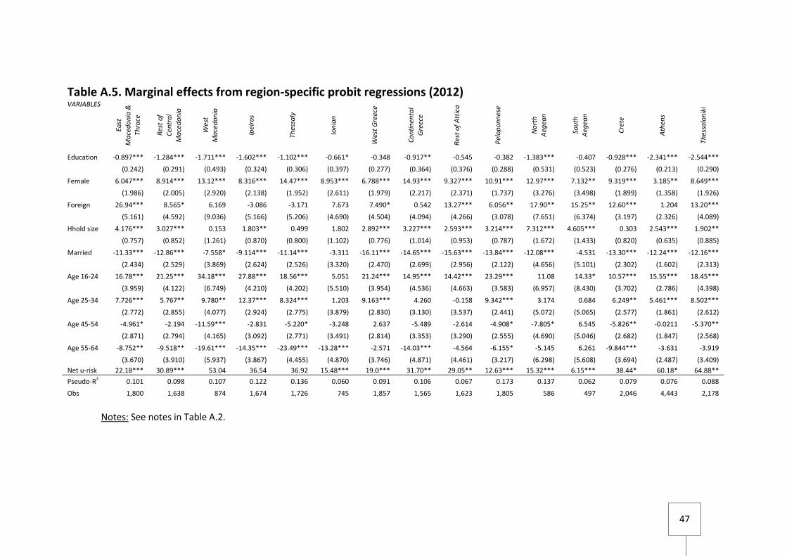
47

Table A.5. Marginal effects from region-specific probit regressions (2012) VARIABLES

East

Ma

ced

on

ia &

Th

race

Res

t o

f C

entr

al

Ma

ced

on

ia

Wes

t M

ace

do

nia

Ipei

ros

Thes

saly

Ion

ian

Wes

t G

reec

e

Co

nti

nen

tal

Gre

ece

Res

t o

f A

ttic

a

Pel

op

on

nes

e

No

rth

A

egea

n

Sou

th

Aeg

ean

Cre

te

Ath

ens

Thes

salo

nik

i

Education -0.897*** -1.284*** -1.711*** -1.602*** -1.102*** -0.661* -0.348 -0.917** -0.545 -0.382 -1.383*** -0.407 -0.928*** -2.341*** -2.544***

(0.242) (0.291) (0.493) (0.324) (0.306) (0.397) (0.277) (0.364) (0.376) (0.288) (0.531) (0.523) (0.276) (0.213) (0.290)

Female 6.047*** 8.914*** 13.12*** 8.316*** 14.47*** 8.953*** 6.788*** 14.93*** 9.327*** 10.91*** 12.97*** 7.132** 9.319*** 3.185** 8.649***

(1.986) (2.005) (2.920) (2.138) (1.952) (2.611) (1.979) (2.217) (2.371) (1.737) (3.276) (3.498) (1.899) (1.358) (1.926)

Foreign 26.94*** 8.565* 6.169 -3.086 -3.171 7.673 7.490* 0.542 13.27*** 6.056** 17.90** 15.25** 12.60*** 1.204 13.20***

(5.161) (4.592) (9.036) (5.166) (5.206) (4.690) (4.504) (4.094) (4.266) (3.078) (7.651) (6.374) (3.197) (2.326) (4.089)

Hhold size 4.176*** 3.027*** 0.153 1.803** 0.499 1.802 2.892*** 3.227*** 2.593*** 3.214*** 7.312*** 4.605*** 0.303 2.543*** 1.902**

(0.757) (0.852) (1.261) (0.870) (0.800) (1.102) (0.776) (1.014) (0.953) (0.787) (1.672) (1.433) (0.820) (0.635) (0.885)

Married -11.33*** -12.86*** -7.558* -9.114*** -11.14*** -3.311 -16.11*** -14.65*** -15.63*** -13.84*** -12.08*** -4.531 -13.30*** -12.24*** -12.16***

(2.434) (2.529) (3.869) (2.624) (2.526) (3.320) (2.470) (2.699) (2.956) (2.122) (4.656) (5.101) (2.302) (1.602) (2.313)

Age 16-24 16.78*** 21.25*** 34.18*** 27.88*** 18.56*** 5.051 21.24*** 14.95*** 14.42*** 23.29*** 11.08 14.33* 10.57*** 15.55*** 18.45***

(3.959) (4.122) (6.749) (4.210) (4.202) (5.510) (3.954) (4.536) (4.663) (3.583) (6.957) (8.430) (3.702) (2.786) (4.398)

Age 25-34 7.726*** 5.767** 9.780** 12.37*** 8.324*** 1.203 9.163*** 4.260 -0.158 9.342*** 3.174 0.684 6.249** 5.461*** 8.502***

(2.772) (2.855) (4.077) (2.924) (2.775) (3.879) (2.830) (3.130) (3.537) (2.441) (5.072) (5.065) (2.577) (1.861) (2.612)

Age 45-54 -4.961* -2.194 -11.59*** -2.831 -5.220* -3.248 2.637 -5.489 -2.614 -4.908* -7.805* 6.545 -5.826** -0.0211 -5.370**

(2.871) (2.794) (4.165) (3.092) (2.771) (3.491) (2.814) (3.353) (3.290) (2.555) (4.690) (5.046) (2.682) (1.847) (2.568)

Age 55-64 -8.752** -9.518** -19.61*** -14.35*** -23.49*** -13.28*** -2.571 -14.03*** -4.564 -6.155* -5.145 6.261 -9.844*** -3.631 -3.919

(3.670) (3.910) (5.937) (3.867) (4.455) (4.870) (3.746) (4.871) (4.461) (3.217) (6.298) (5.608) (3.694) (2.487) (3.409)

Net u-risk 22.18*** 30.89*** 53.04 36.54 36.92 15.48*** 19.0*** 31.70** 29.05** 12.63*** 15.32*** 6.15*** 38.44* 60.18* 64.88**

Pseudo-R2 0.101 0.098 0.107 0.122 0.136 0.060 0.091 0.106 0.067 0.173 0.137 0.062 0.079 0.076 0.088

Obs 1,800 1,638 874 1,674 1,726 745 1,857 1,565 1,623 1,805 586 497 2,046 4,443 2,178

Notes: See notes in Table A.2.

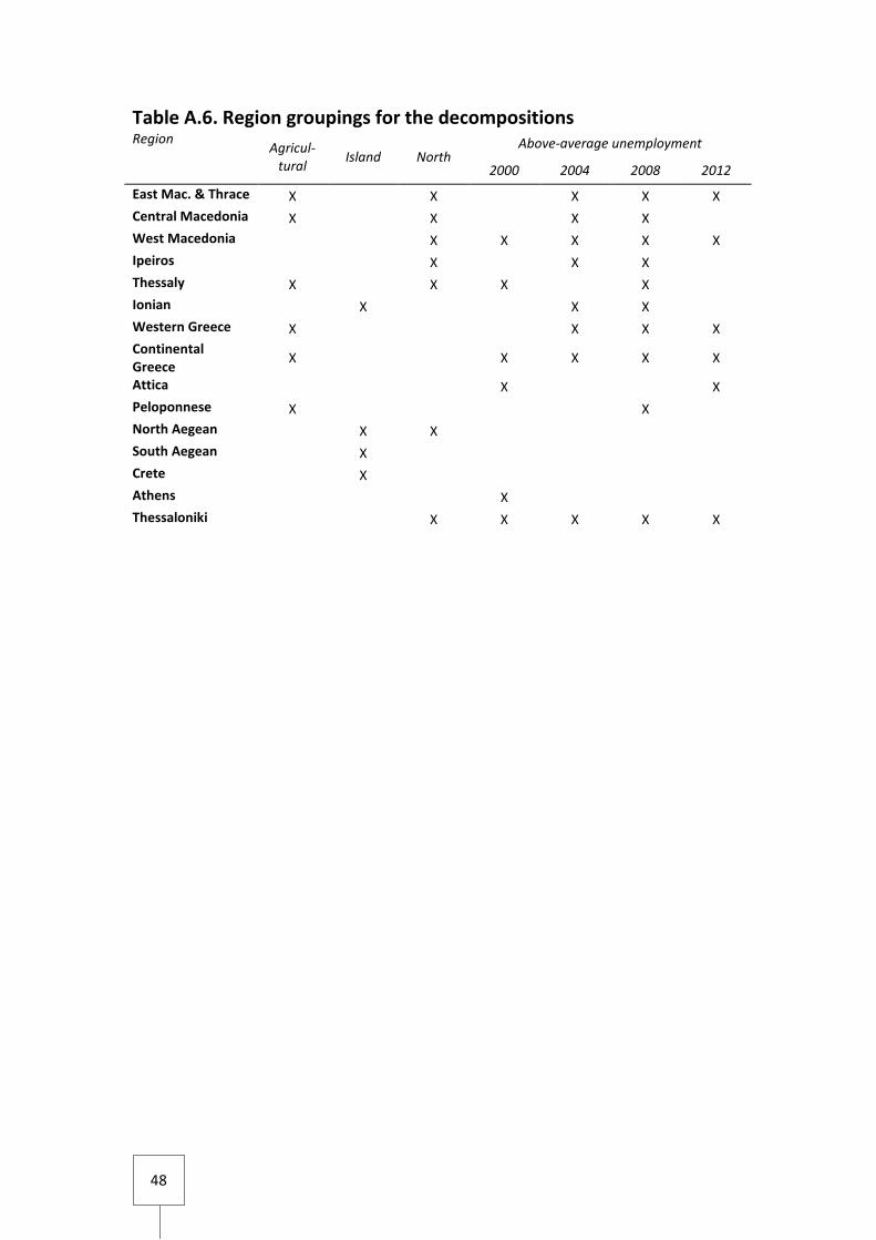
48

Table A.6. Region groupings for the decompositions Region

Agricul-tural

Island North Above-average unemployment

2000 2004 2008 2012

East Mac. & Thrace X

X

X X X

Central Macedonia X

X

X X

West Macedonia

X X X X X

Ipeiros

X

X X

Thessaly X

X X

X

Ionian

X

X X

Western Greece X

X X X

Continental Greece

X

X X X X

Attica

X

X

Peloponnese X

X

North Aegean

X X

South Aegean

X

Crete

X

Athens

X

Thessaloniki

X X X X X

49

References

Ashenfelter O. and Ham J. (1979), Education, unemployment and earnings, Journal of Political Economy 87 (5), pp.S99-S116.

Bakas D. and Papapetrou E. (2012), Unemployment in Greece: evidence from Greek regions, Bank of Greece Working Paper No146, Bank of Greece, Athens.

Bauer T. and Sinning M. (2008), An extension of the Blinder–Oaxaca decomposition to nonlinear models, Advances in Statistical Analysis 92 (2), pp.197-206.

Blackaby D., Leslie D., Murphy P. and O’Leary N. (1999), Unemployment among Britain’s ethnic minorities, The Manchester School 67 (1), pp.1-20.

Cholezas I., Kanellopoulos N., Mitrakos T. and Tsakloglou P. (2012), Unemployment, wages and returns to education in Greece before and during the crisis, paper presented at the Bank of Greece conference “The Greek Labour Market and the Crisis” (November 2012), Bank of Greece.

Christopoulos D. (2004), The relationship between output and unemployment: Evidence from Greek regions, Papers in Regional Science 83 (3), pp.611-620.

Christopoulou R. and Monastiriotis V. (2013), The Greek public sector wage premium before the crisis: size, selection and relative valuation of characteristics, British Journal of Industrial Relations DOI: 10.1111/bjir.12023.

Daouli J., Demoussis M., Giannakopoulos N., and Laliotis I. (2013), The wage curve during the great depression in Greece, mimeo.

Daymont T. and Andrisani P. (1984), Job preferences, college major, and the gender gap in earnings, Journal of Human Resources 19 (3), pp.408-428.

Elhorst J. (2003), The mystery of regional unemployment differentials: theoretical and empirical explanations, Journal of Economic Surveys 17 (5), pp.709-748.

Fairlie R. (2005), An extension of the Blinder-Oaxaca decomposition technique to logit and probit models, Journal of Economic and Social Measurement 30 (2), pp.305-316.

Gomulka J. and Stern N. (1990), The employment of married women in the United Kingdom 1970-83, Economica 57 (1), pp.171-199.

Ham J. and Rea S. (1987), Unemployment Insurance and Male Unemployment Duration in Canada, Journal of Labor Economics 5 (3), pp.325-353.

Heckman J., Lochner L. and Todd P. (2006), Earnings functions, rates of returns and treatment effects: the Mincer equation and beyond, ch.7 in Hanushek E. and Welch F. (eds), Handbook of the Economics of Education, Volume 1, Elsevier, North-Holland.

50

Jann B. (2008), The Blinder-Oaxaca decomposition for linear regression models, The Stata Journal 8 (4), pp.453-479.

Kanellopoulos C. and Mavromatas K. (2002), Male–Female Labour Market Participation and Wage Differentials in Greece, Labour 16 (4), pp.771-801.

Koutentakis F. (2012), Unemployment dynamics in the Greek crisis, Department of Economics Working Paper No1205, University of Crete, Greece.

Livanos I. (2010a), The Wage–Local Unemployment Relationship in a Highly Regulated Labour Market: Greece, Regional Studies 44 (4), pp.389-400.

Livanos I. (2010b), The relationship between higher education and labour market in Greece: the weakest link?, Higher Education 60 (5), pp.473-489.

Livanos I. and Pouliakas K. (2009), The gender wage gap as a function of educational degree choices in an occupationally segregated EU country, IZA Discussion Paper No4636, Institute for the Study of Labor, Bonn.

Lopez-Baso and Motellon (2013), The regional distribution of unemployment. What do micro-data tell us?, Papers in Regional Science 92 (2), pp.383-405.

Mazower M. (2002), The Balkans: a short history, Modern Library Chronicles, Modern House Inc., USA.

McDonald J. and Worswick C. (1997), Unemployment incidence of immigrant men in Canada, Canadian Public Policy 23 (4), pp.353-373.

McGregor A. (1978), Family size and unemployment in a multiply deprived urban area, Regional Studies 12 (3), pp.323-330.

Monastiriotis V. (2009), Examining the consistency of spatial association patterns across socio-economic indicators: an application to the Greek regions, Empirical Economics 37 (1), pp.25-49.

Monastiriotis V. (2011), Making geographical sense of the Greek austerity measures: compositional effects and long-run implications, Cambridge Journal of Society, Economy and Regions, vo.4 (3), pp.323-337.

Nedos V. (2007), Northerners and Southerners, To Vima online (18/11/2007) [in Greek]. Last accessed on 28/7/13 at http://www.tovima.gr/relatedarticles/article/?aid=185036.

Neumark D. (1988), Employers’ discriminatory behavior and the estimation of wage discrimination, Journal of Human Resources 23 (2), pp.279-295.

Oaxaca R. and Ransom M. (1999), ‘Identification in detailed wage decompositions, Review of Economics and Statistics 81 (1), pp.154-157.

Petrakos G. and Psycharis Y. (2004), Regional Development in Greece, Kritiki Publishers, Athens [in Greek].

Solon G. (1979), Labor Supply Effects of Extended Unemployment Benefits, Journal of Human Resources 14 (2), pp.247-255.

51

Stratton L. (1993), Racial differences in men's unemployment, Industrial and Labor Relations Review 46 (3), pp.451-463.

Thurow L. (1975), Generating Inequality, Basic Books, New York. Williams R. (2012), Using the margins command to estimate and interpret

adjusted predictions and marginal effects, The Stata Journal 12 (2), pp.308-331.

Yun M. (2004), Decomposing differences in the first moment, Economics Letters 82 (2), pp.275-280.

Yun M. (2005), A simple solution to the identification problem in detailed wage decompositions, Economic Inquiry 43 (4), pp.766-772.

Previous Papers in this Series

79. Apergis, Nicholas and Cooray, Arusha, New Evidence on the Remedies

of the Greek Sovereign Debt Problem, November 2013

78. Dergiades, Theologos, Milas, Costas and Panagiotidis, Theodore, Tweets, Google Trends and Sovereign Spreads in the GIIPS,

October 2013

77. Marangudakis Manussos, Rontos, Kostas and Xenitidou, Maria, State Crisis and Civil Consciousness in Greece, October 2013

76. Vlamis, Prodromos, Greek Fiscal Crisis and Repercussions for the Property Market, September 2013

75. Petralias, Athanassios, Petros, Sotirios and Prodromídis, Pródromos, Greece in Recession: Economic predictions, mispredictions and policy implications, September 2013

74. Katsourides, Yiannos, Political Parties and Trade Unions in Cyprus, September 2013

73. Ifantis, Kostas, The US and Turkey in the fog of regional uncertainty, August 2013

72. Mamatzakis, Emmanuel, Are there any Animal Spirits behind the Scenes of the Euro-area Sovereign Debt Crisis?, July 2013

71. Etienne, Julien, Controlled negative reciprocity between the state and civil society: the Greek case, June 2013

70. Kosmidis, Spyros, Government Constraints and Economic Voting in Greece, May 2013

69. Venieris, Dimitris, Crisis Social Policy and Social Justice: the case for Greece, April 2013

68. Alogoskoufis, George, Macroeconomics and Politics in the Accumulation of Greece’s Debt: An econometric investigation 1974-2009, March 2013

67. Knight, Daniel M., Famine, Suicide and Photovoltaics: Narratives from the Greek crisis, February 2013

66. Chrysoloras, Nikos, Rebuilding Eurozone’s Ground Zero - A review of the Greek economic crisis, January 2013

65. Exadaktylos, Theofanis and Zahariadis, Nikolaos, Policy Implementation and Political Trust: Greece in the age of austerity, December 2012

64. Chalari, Athanasia, The Causal Powers of Social Change: the Case of Modern Greek Society, November 2012

63. Valinakis, Yannis, Greece’s European Policy Making, October 2012

62. Anagnostopoulos, Achilleas and Siebert, Stanley, The impact of Greek labour market regulation on temporary and family employment - Evidence from a new survey, September 2012

61. Caraveli, Helen and Tsionas, Efthymios G., Economic Restructuring, Crises and the Regions: The Political Economy of Regional Inequalities in Greece, August 2012

60. Christodoulakis, Nicos, Currency crisis and collapse in interwar Greece: Predicament or Policy Failure?, July 2012

59. Monokroussos, Platon and Thomakos, Dimitrios D., Can Greece be saved? Current Account, fiscal imbalances and competitiveness, June 2012

58. Kechagiaras, Yannis, Why did Greece block the Euro-Atlantic integration of the Former Yugoslav Republic of Macedonia? An Analysis of Greek Foreign Policy Behaviour Shifts, May 2012

57. Ladi, Stella, The Eurozone Crisis and Austerity Politics: A Trigger for Administrative Reform in Greece?, April 2012

56. Chardas, Anastassios, Multi-level governance and the application of the partnership principle in times of economic crisis in Greece, March 2012

55. Skouroliakou, Melina, The Communication Factor in Greek Foreign Policy: An Analysis, February 2012

54. Alogoskoufis, George, Greece's Sovereign Debt Crisis: Retrospect and Prospect, January 2012

53. Prasopoulou, Elpida, In quest for accountability in Greek public administration: The case of the Taxation Information System (TAXIS), December 2011

52. Voskeritsian, Horen and Kornelakis, Andreas, Institutional Change in Greek Industrial Relations in an Era of Fiscal Crisis, November 2011

51. Heraclides, Alexis, The Essence of the Greek-Turkish Rivalry: National Narrative and Identity, October 2011

50. Christodoulaki, Olga; Cho, Haeran; Fryzlewicz, Piotr, A Reflection of History: Fluctuations in Greek Sovereign Risk between 1914 and 1929, September 2011

49. Monastiriotis, Vassilis and Psycharis, Yiannis, Without purpose and strategy? A spatio-functional analysis of the regional allocation of public investment in Greece, August 2011

SPECIAL ISSUE edited by Vassilis Monastiriotis, The Greek crisis in focus: Austerity, Recession and paths to Recovery, July 2011

48. Kaplanoglou, Georgia and Rapanos, Vassilis T., The Greek Fiscal Crisis and the Role of Fiscal Government, June 2011

47. Skouras, Spyros and Christodoulakis, Nicos, Electoral Misgovernance Cycles: Evidence from wildfires and tax evasion in Greece and elsewhere, May 2011

46. Pagoulatos, George and Zahariadis, Nikolaos, Politics, Labor, Regulation, and Performance: Lessons from the Privatization of OTE, April 2011

45. Lyrintzis, Christos, Greek Politics in the Era of Economic Crisis: Reassessing Causes and Effects, March 2011

44. Monastiriotis, Vassilis and Jordaan, Jacob A., Regional Distribution and Spatial Impact of FDI in Greece: evidence from firm-level data, February 2011

43. Apergis, Nicholas, Characteristics of inflation in Greece: mean spillover effects among CPI components, January 2011

42. Kazamias, George, From Pragmatism to Idealism to Failure: Britain in the Cyprus crisis of 1974, December 2010

41. Dimas, Christos, Privatization in the name of ‘Europe’. Analyzing the telecoms privatization in Greece from a ‘discursive institutionalist’ perspective, November 2010

40. Katsikas, Elias and Panagiotidis, Theodore, Student Status and Academic Performance: an approach of the quality determinants of university studies in Greece, October 2010

Online papers from the Hellenic Observatory

All GreeSE Papers are freely available for download at http://www2.lse.ac.uk/ europeanInstitute/research/hellenicObservatory/pubs/GreeSE.aspx

Papers from past series published by the Hellenic Observatory are available at http://www.lse.ac.uk/collections/hellenicObservatory/pubs/DP_oldseries.htm