Embed Size (px)
Citation preview
JID:TCS AID:9537 /FLA Doctopic: Algorithms, automata, complexity and games [m3G; v 1.117; Prn:2/12/2013; 15:44] P.1 (1-18)
Theoretical Computer Science ••• (••••) •••–•••
Contents lists available at ScienceDirect
Theoretical Computer Science
www.elsevier.com/locate/tcs
Bi-criteria and approximation algorithms for restrictedmatchings ✩
Monaldo Mastrolilli, Georgios Stamoulis ∗
Istituto Dalle Molle di Studi sull’Intelligenza Artificiale, IDSIA (USI/SUPSI), Manno-Lugano, Switzerland
a r t i c l e i n f o a b s t r a c t
Keywords:Approximation algorithmsCombinatorial optimizationLinear programmingGraph algorithms
In this work we study approximation algorithms for the Restricted matching problem whichis defined as follows: given a graph in which each edge e has a color ce and a profitpe ∈ Q+, we want to compute a maximum (cardinality or profit) matching in which nomore than w j ∈ Z+ edges of color c j are present. This kind of problems, beside thetheoretical interest on its own right, emerges in multi-fiber optical networking systems,where we interpret each unique wavelength that can travel through the fiber as a colorclass and we would like to establish communication between pairs of systems. We studyapproximation and bi-criteria algorithms for this problem which are based on linearprogramming techniques and, in particular, on polyhedral characterizations of the naturallinear formulation of the problem. In our setting, we allow violations of the bounds w j andwe can model our problem as a bi-criteria problem: we have two objectives that we wantto optimize namely (a) to maximize the profit (maximum matching) while (b) minimizingthe violation of the color bounds. We prove how we can “beat” the integrality gap of thenatural linear programming formulation of the problem by allowing only a slight violationof the color bounds. In particular, our main result is constant approximation bounds forboth criteria of the corresponding bi-criteria optimization problem.
© 2013 Elsevier B.V. All rights reserved.
1. Introduction
Consider the following game: we organize a competition in a school and we have a set of binary games such as chess,GO, tavli (a.k.a. backgammon), etc. Some pairs of students are interested in playing one particular game, whereas some otherpairs are interested in some other game. We only have a limited amount of free boards for a particular game. Ideally, wewould like to satisfy as many pairs of students as possible with the available amount of boards. This simple game capturesexactly the essence of the problem of this article: we can formulate the above scenario as a graph G = (V , E), where Vis the set of students, and two students that are interested in a particular game (say chess) are connected with an edgeof a particular color (say black) associated with this game. Let w j ∈ N be the number of available boards of game j. Thenthe task of the organizers is to compute a maximum matching that uses at most w j boards of game j. Call this problemBounded Color Matching problem.
More formally, the problem can be stated as follows:
✩ A preliminary version of this work appeared in Proceedings of the 2nd International Symposium on Combinatorial Optimization (ISCO 2012), Lecture Notesin Computer Science. Supported by the Swiss National Science Foundation Project No. 200020-122110/1 “Approximation Algorithms for Machine SchedulingThrough Theory and Experiments III” and by Hasler Foundation Grant 11099.
* Corresponding author.E-mail addresses: [email protected] (M. Mastrolilli), [email protected] (G. Stamoulis).
0304-3975/$ – see front matter © 2013 Elsevier B.V. All rights reserved.http://dx.doi.org/10.1016/j.tcs.2013.11.027
JID:TCS AID:9537 /FLA Doctopic: Algorithms, automata, complexity and games [m3G; v 1.117; Prn:2/12/2013; 15:44] P.2 (1-18)
2 M. Mastrolilli, G. Stamoulis / Theoretical Computer Science ••• (••••) •••–•••
Definition 1 (Bounded Color Matching). We are given a (simple, un-directed) graph G = (V , E) with vertex set V and edgeset E such that |V | = n and |E| = m. The edge set is partitioned into k sets E1 ∪ E2 ∪ · · · ∪ Ek i.e. every edge e has colorC j if e ∈ E j and a profit pe ∈ Q+ . We are asked to find a maximum (weighted) matching M (or a matching of maximumcardinality) such that in M there are no more that w j edges of color C j , where w j ∈ Z+ i.e. a matching M such that|M ∩ E j | � w j , ∀ j ∈ [k].
In the following, we denote as C the collection of all the color classes. In other words, C = {C j} j∈[k] . Moreover, for agiven edge e ∈ E(G), we denote by c(e) its color i.e. c(e) = C j ⇔ e ∈ E j .
Besides the previously mentioned toy problem, Bounded Color Matching emerges in optical networking systems: in anoptical fiber we allow multiplexing of different frequencies (i.e. different beams of light can travel at the same time insidethe same fiber), but we have limited capacities of the number of light beams of a particular frequency that we allow to travelsimultaneously through the system, due to potential interference problems. We would like to establish connections betweena maximum number of (disjoint) pairs of systems while at the same time respecting the maximum number of connectionsusing the same frequency we allow in multiplexing. Moreover, the Bounded Color Matching problem with 2 colors (i.e. thecase that each edge is colored either blue or red) can be used in approximately solving the Directed Maximum Routingand Wavelength Assignment problem (DirMRWA) [44] in rings which are fundamental network topologies, see [45] (also [8,9] for alternative and slightly better approximation algorithms and [3] for combinatorial algorithms). Here, approximatelysolving means that an (asymptotic) α-approximation algorithm for maximum blue–red matching results in an (asymptotic)α+1α+2 -approximation algorithm for DirMRWA in rings.
1.1. History and related results
Characterizations and algorithms for maximum matchings in graphs have a very long history. One of the first attemptsto characterize the structure of matchings was as early as the 1957 when Claude Berge characterized the structure ofmaximum matchings with respect to alternating and augmenting paths [5]: a matching M on a given graph G is maximumif and only if G contains no M-augmenting paths. A path that alternates between edges in M and edges not in M (fora given matching M) is called an M-alternating path. An M-alternating path whose endpoints are unsaturated by M (i.e.vertices that do not have edges incident to them that are in M) is called an M-augmenting path. M-augmenting pathsprovide a certificate of the non-maximality of M .
Given this characterization of maximum matchings, an algorithm is immediate for computing a maximum matching Mon a graph G:
Initialize M := ∅while there exists an M-augmenting path Pdo augment M along P .
Of course the running time of the above general algorithm depends on how fast we can find M-augmenting pathson a graph G with m edges and n vertices. In case the graph is bipartite finding maximum matchings can be done (rel-atively) easily in time O(m
√n) [28,29], beating the “trivial” brute-force approach which simply enumerates all possible
M-augmenting paths which takes time O(nm). We remind that a graph G is bipartite if its vertex set can be partitionedinto two sets V 1, V 2 such that every edge connects a vertex in V 1 to one in V 2; that is, V 1 and V 2 are independent sets.Equivalently, a bipartite graph is a graph that does not contain any odd-length cycles.
The case when G is not bipartite is significantly more complicated because of the presence of odd-length cycles. In hisseminal 1965 article, Jack Edmonds presented an O(n2m) time algorithm for solving the maximum matching problemin general graphs [17]. In fact, it was precisely this article that introduced the concept of polynomially time solvable prob-lems as “tractable” problems. As it always happens, the running time of this algorithm has been significantly improvedover the years. In [18], by a sophisticated use of some data structures, a running time of min{√nm log n,n2.5} was shownfor computing a maximum matching in a graph G , which was later improved to O(n2.5), see [40].
The previous algorithms are purely combinatorial. Other very successful approaches for computing maximum matchingsin graphs are based on using of algebraic methods and/or randomization. We will not go into much detail here, exceptmentioning the most important results, which include an O(nω+1) time algorithm [47], and two O(nω) time algorithms[43] and [26] (see also [27]), where ω = inf{c: two n × n matrices can be multiplied in time O(nc)} (we note that ω �log2 7 2.38).
All the above algorithms work for the un-weighted (uniform weights) case. In case we have a weight function w : E →Q+and we want to compute a maximum weighted matching, then other techniques are required. The most common techniqueis the so-called Hungarian method [32], which is a primal–dual technique, initially introduced for bipartite graphs. For generalgraphs, similar primal–dual techniques have been employed, see for example [16,19–21] among others. The idea, as most ofthe primal–dual schemata, is to build up feasible primal and dual solutions simultaneously and show that at the end bothsolutions satisfy complementary slackness conditions and hence by the duality theorem, the primal solution is a maximumweight matching. Another approach for the maximum weight matching problem is to maintain a feasible matching and
JID:TCS AID:9537 /FLA Doctopic: Algorithms, automata, complexity and games [m3G; v 1.117; Prn:2/12/2013; 15:44] P.3 (1-18)
M. Mastrolilli, G. Stamoulis / Theoretical Computer Science ••• (••••) •••–••• 3
try to successively augment it to increase its weight, until no more augmenting is possible, see for example [15]. Forcomprehensive accounts of the matching problem, we refer to [37] and [49].
1.2. Constrained matching problems
Since the task of computing maximum matchings is an extremely well studied and basic problem, the interest hasshifted towards some other versions of maximum matchings, in particular to versions where we seek a maximum matchingsubject to additional criteria (constraints). These criteria reduce the feasible solution space, making it (usually) harder tocompute optimal solutions in polynomial time. In this direction, Bounded Color Matching problems were studied as earlyas the 1970s as a very interesting generalization of the classical maximum matching problem: In [22], the problem wasdefined as Multiple Choice Matching (reference problem [GT55]) and proved to be NP-complete even for the very special casewhere the graph is bipartite, each color class contains at most 2 edges (i.e. |E j| � 2, ∀ j) and w j = 1, ∀C j ∈ C . This problem,finds numerous practical applications, from classroom scheduling to image segmentation among others, see also [30,31].
Moreover, the uniform weight version of Bounded Color Matching problem is also closely related to the Labeled Matchingproblem [42,11] in which all bounds w j are set equal to 1, i.e. we would like a maximum matching with at most one edgeper color. In [42] it was proven that even the very special case of 2-regular bipartite graphs where each color appears twice(i.e. in at most two edges), the problem is APX-hard and so a PTAS is immediately out of reach for Bounded Color Matching(see also [41]).
Budgeted versions of the maximum matching problem, have been recently studied intensively. Here, by budgeted versionof a combinatorial optimization problem Π we mean the following: Besides the profit function p : F → Q+ associatedwith every feasible solution F ∈ F for Π (where F is the set of all feasible solutions for Π ), we are also given a set of �
cost functions {�i}i∈[�] such that �i : F → Q+ , and for every cost function �i a budget βi ∈ Q+ . The budgeted optimizationversion of Π , which we call Πb , can be then formulated as follows (assuming that Π is a maximization problem):
max p(F ), subject to F ∈ F and ρi(F ) � βi, ∀i ∈ [�]. (1)
In [24] (see also [25]) the authors considered the 2-budgeted maximum matching problem (i.e. the case where � = 2)and devised a PTAS. This algorithm works roughly as follows: First of all, a guessing step is performed that guesses the1/ε most valuable edges of the optimal matching. Then, an optimal fractional matching x∗ is computed for the rest of thegraph (for example by solving the linear programming relaxation of the problem). By Carathéodory’s theorem [10], x∗ canbe written as a convex combination of at most three (possibly unfeasible) matchings i.e. x∗ = λ1x1 + λ2x2 + (1 − λ1 − λ2)x3.Then, the algorithm consists of two “merging” steps: in the first step, given the first two matchings x1 and x2 the output is athird matching z with comparable profit and which is not costlier than μx1 + (1 − μ)x2 for μ = λ1
λ1+λ2with respect to both
the two extra cost functions. Then the same procedure is again applied to z and x3 with parameter μ = λ1+λ2λ1+λ2+(1−λ1−λ2)
, i.e.we merge x3 with z such that the new matching z∗ is feasible (with respect to both cost functions) and (almost) optimal.
This was further improved in [13] where it is given a PTAS for a fixed number of budgets. The authors there providedboth randomized and deterministic PTAS’s for the problem. The randomized version is based on strong concentration boundsof some suitable martingale processes (see also [12] for some closely related results and techniques). The deterministic PTAScan be seen as a bi-criteria approximation, and the final solution returned is within (1 − ε) the optimal but it might violatethe budgets by a factor of (1 + ε) (i.e. the solution z returned has the property that ci(z) � (1 + ε)βi , ∀i). Moreover, forunbounded number of budgets the authors prove an almost optimal approximation guarantee, but with allowing a verylarge (i.e. logarithmic) overflow on the budgets (as before, this means that for the computed solution z, z has the propertythat ci(z) � βi logβi , ∀ budget i). These results generalize the results for the budgeted bipartite matching problem, for whicha PTAS was known for the case of one budget [6,7], or in the case of fixed number of budgets [23] in which a (1 − ε,1 + ε)
bi-criteria approximation was shown.To the best of our knowledge, the first case where matching problems with cardinality (disjoint) budgets were consid-
ered, was in [45] where the authors defined and studied the blue–red Matching problem: compute a maximum (cardinality)matching that has at most w blue and at most w red edges, in a blue–red colored (multi)-graph. A 3
4 polynomial timecombinatorial approximation algorithm and an RNC2 algorithm were presented (that computes the maximum matchingthat respects both budget bounds with high probability). We note that the exact complexity of the blue–red matching prob-lem is not known: it is only known that blue–red matching is at least as hard as the Exact Matching problem [46] whosecomplexity is open for more than 30 years. A polynomial time algorithm for the blue–red matching problem will imply thatExact Matching is polynomial time solvable. On the other hand, blue–red matching is probably not NP-hard since it ad-mits an RNC2 algorithm. We note that this algorithm can be extended to a constant number of color classes with arbitrarybounds w j . Using the results of [53] (also appeared in [52]) one can deduce an “almost” optimal deterministic algorithmfor blue–red matching, i.e. an algorithm that returns a matching of maximum cardinality that violates the two color boundsby at most one edge. This is the best possible, unless of course blue–red matching (and, consequently, exact matching) arein P.
JID:TCS AID:9537 /FLA Doctopic: Algorithms, automata, complexity and games [m3G; v 1.117; Prn:2/12/2013; 15:44] P.4 (1-18)
4 M. Mastrolilli, G. Stamoulis / Theoretical Computer Science ••• (••••) •••–•••
1.3. Our contributions
In this article we study the Bounded Color Matching problem, from a Linear Programming point of view. In particular, weare interested how good approximation algorithms we can design using linear programming methods. The main contributionof the current manuscript is to show how we can “beat” the integrality gap of the natural LP formulation of the BCMproblem, allowing small violation of the color bounds w j .
Before we do that, we firstly prove that a simple greedy and fast procedure gives a 13 approximate solution. To prove the
approximation guarantee of this simple procedure, we use a characterization that was introduced in [39] to show that ourproblem falls into the framework of �-extendible systems. This serves the purpose of a baseline and “warm-up” result.
Then we design and analyze various algorithms based on Linear Programming techniques. Our algorithms are based oniterative rounding of basic (fractional) feasible solutions of the natural Linear Programming formulation of the Bounded ColorMatching problem. We employ a fractional charging technique (introduced in [4]) to characterize the structure of extremepoint solutions of the LP relaxation of our problem. Taking advantage of this structure, we provide bi-criteria additiveand multiplicative approximation algorithms for both the weighted and un-weighted case (see [51] and also [35] for acomprehensive account of the applications of iterative rounding techniques in the context of combinatorial optimization).
Very generally, our algorithms have two (global) steps:
– Either (iteratively) apply a rounding step on some variable with high fractional value in such a way that the resultingsolution remains feasible, or
– apply a relaxation step in which we decide to drop a budget constraint if a constraint with “few” non-zero variablesexists.
Our results (and the structure of this document) can be summarized as follows:
1. Firstly, as already mentioned, we show that a straightforward greedy strategy results in a 13 -approximation guarantee.
2. In the next section we prove some combinatorial properties of the natural linear programming formulation and weapply these techniques in the special case of the BCM problem where w j = 1, ∀ j ∈ [k]. We note that this case remainsAPX-hard (see related work section). We provide an asymptotic approximation of the optimal objective function valueby allowing a small additive violation of the color bounds w j . In particular we prove that there exists a polynomial timealgorithm that, for any α ∈ Z+ (in fact we require that α is greater than 3 on bipartite and greater than 4 in generalgraphs), it computes a matching of value at least opt(1 − 4
α ) + 1α + 1 that has at most α edges of every color (where
opt is the optimal solution value). This result can be improved to opt(1 − 3α ) + 1
α + 1 with the same additive α − 1violation bound in case the graph is bipartite. This means that, by allowing a moderate additive violation of α − 1 forevery color class, we can approximate the optimal objective function value within any precision (that depends on α).The result holds for the uniform weight case.
3. Then, we further investigate some properties of the underlying polyhedron and using these properties we show howwe can in fact obtain a family of bi-criteria approximation algorithms with varying guarantees. In particular, we provethe following:(a) There exists a 1
2 -approximation algorithm for the weighted version of the BCM problem, allowing only an additiveone violation of the color bounds w j .
(b) We prove that, for any λ ∈ [0,1], there is a polynomial time ( 23+λ
, 21+λ
+ 1w j
) bi-criteria approximation algorithm
for the un-weighted Bounded Color Matching problem i.e. we prove constant approximation bounds with respectto both criteria. We note that, to the best of our knowledge, this is the first result that provides such performanceguarantees (compare with the (1 − ε) approximation but with logarithmic budget violation of [13]).
(c) Finally, we present a polynomial time 12 approximation algorithm for the uniform weight Bounded Color Matching
problem without any violation of the color budgets, matching the integrality gap of the natural linear relaxation ofthe problem.
2. Preliminaries and theoretical framework
Consider the classical matching problem on a general graph G = (V , E). If we introduce binary variables xe , ∀e = {u, v} ∈E(G) where xe = 1 ⇔ e ∈ M , then we can describe the problem of finding a maximum matching with a linear program asfollows: find a vector x ∈ {0,1}|E| that maximizes 1T x (or pT x for a general profit vector p ∈ Q|E|
+ ) such that adjacent toeach vertex, there is at most one variable (edge) that takes the value one. In particular, the linear program is the following:{
max pT x, s.t.∑
e∈δ(v)
xe � 1, ∀v ∈ V , x ∈ {0,1}|E|}
(2)
where δ(v) = {e ∈ E(G): v ∈ e}, ∀v ∈ V (G). The constraint of the form∑
e∈δ(v) xe � 1, ∀v ∈ V , simply tells us that we seeka solution that has at most one edge incident to every vertex of the graph. Unfortunately, solving this integer program is
JID:TCS AID:9537 /FLA Doctopic: Algorithms, automata, complexity and games [m3G; v 1.117; Prn:2/12/2013; 15:44] P.5 (1-18)
M. Mastrolilli, G. Stamoulis / Theoretical Computer Science ••• (••••) •••–••• 5
NP-hard. The usual thing to do it to relax the integrality constraints of the variables, i.e., replace the constraint x ∈ {0,1}|E|with the x ∈ [0,1]|E| . This relaxed program can be solved in polynomial time [48]. The problem is that, in general, solvingthe relaxation of an integer program results in a fractional vector. In some cases, we are able to add some valid constraintsthat cause the solution to be always integer, and this is the case with the maximum matching problem in general graphs:the problem is caused by structures called blossoms i.e. holes (cycles) of odd cardinality. Let S be such a cycle of cardinality|S|, which is an odd number. Any maximum matching can contain at most |S|−1
2 edges from this cycle, but the linear
programming relaxation can assign value 12 to every edge of the cycle for a fractional vector of value |S|
2 >|S|−1
2 . To solvethis, we add the so-called blossom inequalities that constraint exactly this: in every odd cycle, we require that the sum ofthe values assigned to its edges is at most |S|−1
2 and this result to the following restricted polyhedron: Find x ∈ [0,1]|E| thatmaximizes pT x such that{ ∑
e∈δ(v)
xe � 1, ∀v ∈ V ,∑
e∈E(S)
xe �|S| − 1
2, ∀S ⊆ V , |S| odd cardinality
}(3)
where by E(S) for S ⊆ V we denote the set of edges included in the graph induced by the vertex set S . Although theabove linear program described in (3) has exponential number of constraints for general graphs (one for every vertex andone for every odd sized subset of vertices), we can still solve it in polynomial time by the Ellipsoid method if we provide aseparation oracle, which for any given candidate solution vector x ∈ [0,1]|E| will either respond that x is a feasible solutionfor the linear programming inequalities defined above, or, it will respond that x is infeasible by providing the violatedconstraint. A very interesting fact is that by solving this linear relaxation, the resulting vector is always integral!
These “blossom” constraints are redundant in case of bipartite graphs (since in bipartite graphs every cycle is of evenlength), but are essential in our general graph setting. So, when we consider bipartite graphs we will assume that theseconstraints will not be part of the LP and we will be just using the initial degree-constrained polyhedron described by (2).Again here we have the phenomenon that by solving the linear relaxation, the resulting vector is again integral [49,14,15,37].
Call the polyhedron that contains all feasible points of (3) or (2) as M. We use the same name for both polyhedra, butfrom the context will be clear which one we are using, thus avoiding any confusion. For a comprehensive treatment of thevarious properties of M, including a polynomial time separation oracle, we refer to [37].
We can describe the set of all feasible solution of the constrained (Bounded Color) matching problem as follows:
Mc ={
y ∈ {0,1}E : y ∈ M∧∑e∈E j
ye � w j, ∀ j ∈ [k]}. (4)
To judge the quality of a linear programming relaxation, and to explore the limits of linear programming techniques,it has been introduced the concept of integrality gap (or integrality ratio): informally a linear relaxation is strong when itdoes not allow a lot of “cheating” with regard the objective function value over the original integral formulation. This iscalled integrality gap and is defined as follows: Let us assume that we have an optimization problem with a set of validinstances I and let Z the set of all feasible solutions for a particular instance ∈ I defined by the integer formulation ofthe problem which we call it IP. Define opt(IP) = opt(Z) = maxz∈Z f (z) where f (z) is the objective function value of thefeasible solution z. As before, let Z ′ be the set of feasible points on the linear relaxation of IP (which we call it LP) anddefine opt(LP)opt(Z ′) = maxq∈Z ′ f (q). Then the integrality gap (or the integrality ratio) of the relaxation of IP is
supi∈I
opt(LP)
opt(IP).
Of course, the closer this quantity is to one, the better the quality of the formulation. An LP formulation with integralitygap of � implies that it is impossible to design an approximation algorithm with performance guarantee better than � usingthis particular formulation as upper/lower bounding schema for our discrete optimization problem.
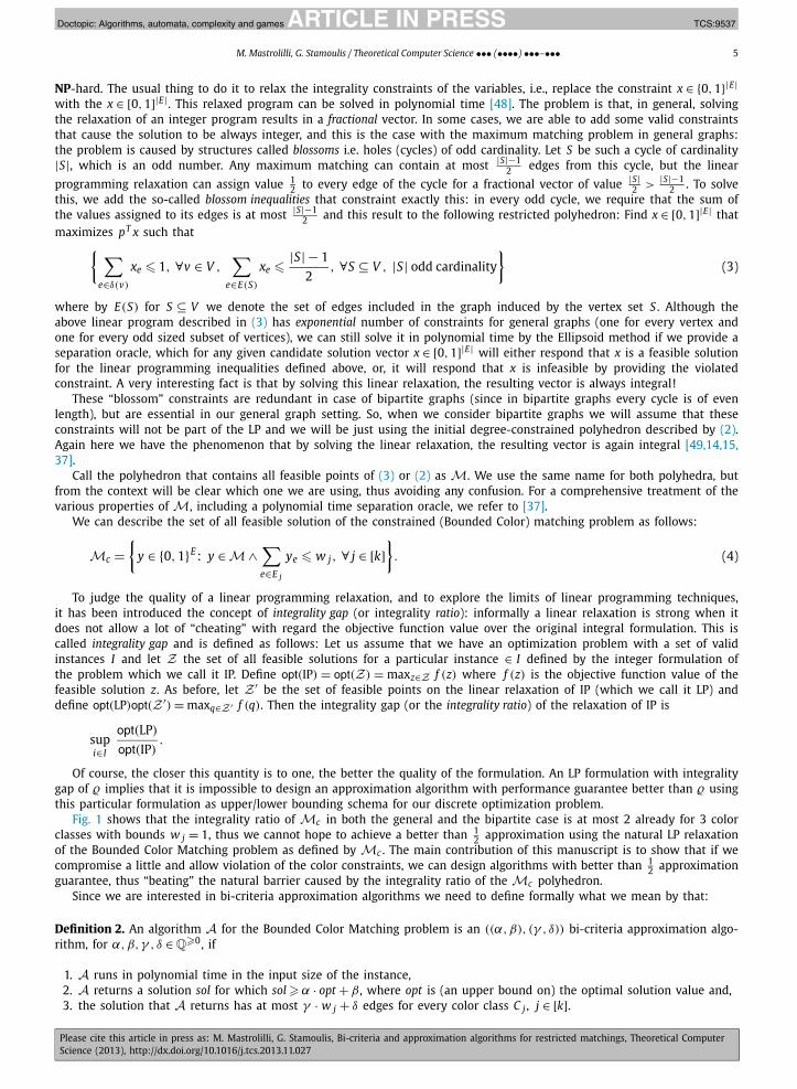
Fig. 1 shows that the integrality ratio of Mc in both the general and the bipartite case is at most 2 already for 3 colorclasses with bounds w j = 1, thus we cannot hope to achieve a better than 1
2 approximation using the natural LP relaxationof the Bounded Color Matching problem as defined by Mc . The main contribution of this manuscript is to show that if wecompromise a little and allow violation of the color constraints, we can design algorithms with better than 1
2 approximationguarantee, thus “beating” the natural barrier caused by the integrality ratio of the Mc polyhedron.
Since we are interested in bi-criteria approximation algorithms we need to define formally what we mean by that:
Definition 2. An algorithm A for the Bounded Color Matching problem is an ((α,β), (γ , δ)) bi-criteria approximation algo-rithm, for α,β,γ , δ ∈Q�0, if
1. A runs in polynomial time in the input size of the instance,2. A returns a solution sol for which sol � α · opt + β , where opt is (an upper bound on) the optimal solution value and,3. the solution that A returns has at most γ · w j + δ edges for every color class C j , j ∈ [k].
JID:TCS AID:9537 /FLA Doctopic: Algorithms, automata, complexity and games [m3G; v 1.117; Prn:2/12/2013; 15:44] P.6 (1-18)
6 M. Mastrolilli, G. Stamoulis / Theoretical Computer Science ••• (••••) •••–•••
Fig. 1. Two examples of bad integrality gap: In the first graph, edges {v1, v2}, {v3, v4} are blue and edges {v1, v4}, {v2, v3} are red. In the second graphedges {u1, u3}, {u2, u4} are blue, edges {u1, u2}, {u3, u4} are green and edges {u1, u4}, {u2, u3} are red. In both cases we seek a maximum matching with atmost 1 edge per color. Any optimal integral solution has value 1 in both graphs. Observe that in the first case the all 1
2 solution gives a solution of value 2
but every integral optimal solution has value 1. The same is true in the second graph which is not bipartite: by assigning the value 13 to all the edges we
get an optimal solution of value 2 (note that the all 13 solution is not a basic feasible solution). (For interpretation of the references to color in this figure
legend, the reader is referred to the web version of this article.)
In the following lemma, we show that using linear programming techniques, it is impossible to design bi-criteria ap-proximation algorithms with certain performance guarantees, even for very simple cases. In particular, we show that it isimpossible to obtain an additive error with the natural LP formulation without violating the objective function value.
Lemma 1. It is impossible to design bi-criteria approximation algorithms for the BCM problem of the form ((1,0), (0, ζ )), for anyadditive value of ζ using the natural linear programming formulation of the problem.
Proof. Consider the following instance of the BCM problem: we are given a (bipartite) graph G = (V , U , E) with bipartitionU , V on 2n vertices (|V | = |U | = n) which is actually a path i.e. E = (vi, ui) ∪ (vi+1, ui)i=1,...,n . We have only one budget ofthe form
∑e∈R xe � n
2 where R = (vi, ui)i=1,...,n . We solve the linear program (4) to obtain an optimal basic solution x. Thisbasic feasible solution corresponds to the vector x = (1/2, . . . ,1/2)T . So, in this example, the number of fractional edges forthe cardinality constraint is n which is twice as much as the bound of the constraint which proves that there are not alwaysconstraints that have “few” non-zero variables. On the other hand, observe that the optimal (fractional) solution has value of2n−1
2 since we have 2n − 1 edges (a path on 2n vertices) and each edge get value 12 . On the other hand, even after dropping
the budget constraint by the edges defined by R , the optimal (integral) solution has value n−22 and so we cannot “reach”
the optimal fractional solution. In other words, we cannot hope to achieve any additive violation on the budget constraint,for any constant value, without violating the objective function. �
And so, we have to “violate” the objective function value (i.e. settle for an approximate solution) if we wish to achieve aconstant violation on the color bounds. Please relate this impossibility result with the result of [53] where it is shown howto compute, via combinatorial methods, maximum matchings with at most an additive one violation of the color budgets,for two color classes.
3. A greedy 1/3 approximation algorithm
In this section we consider the weighted variant of the Bounded Color Matching problem where each edge e has a profitpe ∈ Q+ . The goal is to find a maximum profit matching that respects the color bounds. Here we show how an O(|E| log |E|)greedy procedure can easily derive a 1
3 approximation for general weighted graphs.
Algorithm 1 Greedy algorithm for Bounded Color Matching problem.Input: Graph G = (V , E), a color function c : e → [k], a profit function p : e →Q+ .Output: A matching M such that |M ∩ E j | � w j , ∀ color class j ∈ [k].
1. initialize M := ∅.2. Sort all edges of the graph according to their profits in non-increasing order.3. while E(G) �= ∅ do:
– Pick the edge e with the largest profit.– M := M ∪ {e}. wc(e) := wc(e) − 1. E(G) := E(G) \ {e′ ∈ E: e ∩ e′ �= ∅}.– if wc(e) = 0 then remove all edges of the same color from the graph.
4. return M .
To analyze the performance guarantee of the above simple procedure, we will use the notion of �-extendible systemsdue to Mestre [39]:
Definition 3. A subset system is a pair (E,L), where E is a finite ground set of elements and L ⊆ 2E with the propertythat L ∈L⇒ L′ ∈L, ∀L′ ⊂ L. We say that L1 ∈L is an extension of L2 ∈L if L2 ⊆ L1.
JID:TCS AID:9537 /FLA Doctopic: Algorithms, automata, complexity and games [m3G; v 1.117; Prn:2/12/2013; 15:44] P.7 (1-18)
M. Mastrolilli, G. Stamoulis / Theoretical Computer Science ••• (••••) •••–••• 7
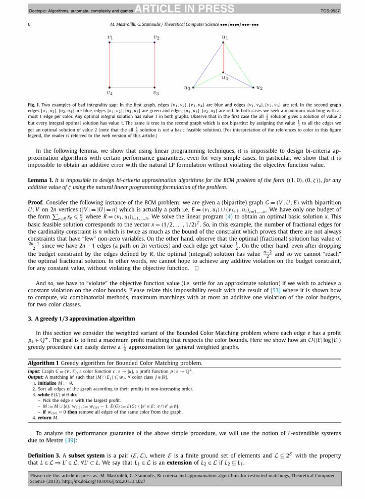
Fig. 2. An example of worst case behavior of the Greedy procedure. Assume that all the color bounds are set to 1. Edges {v1, u3} and {v2, u2} are bluewhile {v1, u1} is red and {v3, u3} is green. Selecting the (blue) edge (v1, u3) will result to a solution of value 1. On the other hand the optimal solutionconsists of selecting the edges (u1, v1), (u2, v2), (u3, v3). (For interpretation of the references to color in this figure legend, the reader is referred to theweb version of this article.)
A subset system (E,L) is said to be �-extendible if ∀X ∈ L, x /∈ X with X ∪ {x} ∈ L and for every extension Y of X ,∃ Y ′ ⊆ Y \ X with |Y ′| � � such that Y \ Y ′ ∪ {x} ∈L.
What is helpful, is the fact that the greedy algorithm applied to �-extendible systems provides a 1�
factor approximation.The following result is from [39]:
Theorem 1. Let (E,L) be an �-extendible system. Then the Greedy algorithm applied to such systems provides a 1�
approximationalgorithm for the optimization problem for any weight (or profit) function p.
Lemma 2. The subset system associated with the Bounded Color Matching problem is 3-extendible.
Proof. Let M and M ′ be feasible solutions such that M ′ is an extension of M (i.e. M ⊆ M ′). Let M be such that M ∪ {e}is still feasible, for some edge e = {u, v} ∈ E with color j such that e /∈ M ′ . By the above property that M ∪ {e} is feasible,it is easy to see that degM(u) = degM(v) = 0 and |M ∩ E j| < w j . Now consider the extension of M , namely M ′ . We canfind at most 3 edges e1, e2, e3 ∈ M ′ such that u ∈ e1, v ∈ e2 and c(e3) = c(e). Observe that we can find many edges e3. Butany such edge would suffice. The point is that the addition of e in M ′ would potentially lead to at most three “conflicting”edges (the addition of e would cause the removal of at most three edges in order the new solution to remain feasible).Consider the new solution Z = M ′ \ {e1, e2, e3} ∪ e. This is still a feasible solution for the Bounded Color Matching problemwith |{e1, e2, e3}| � 3 = �, and so the system characterizing our problem is 3-extendible. Observe that we use inequality inthe |{e1, e2, e3}| � 3 because it might be, for example, that e1 = e3. �Corollary 1. Algorithm 1 is an O(m log m) time 1
3 -approximation algorithm for the weighted version of the Bounded Color Matchingproblem in general graphs.
Fig. 2 shows that this bound is essentially tight.
4. Combinatorial properties of the Mc polyhedron
In this subsection we will prove some interesting combinatorial properties of extreme point solutions of the polyhe-dron Mc . Later on, we will take advantage of these properties to devise our approximation algorithms. We first need somepreliminary definitions.
Definition 4. Let E ′ ⊆ E be a subset of the edges of the graph. Then, we define the characteristic vector of E ′ to be thebinary vector χE ′ ∈ {0,1}E such that χE ′ (e) = 1 ⇔ e ∈ E ′ i.e. the ith component of χE ′ is 1, if the ith edge belongs to E ′ andzero otherwise.
Definition 5. Let y be a real-valued vector in an n-dimensional space. Define the support of y to be the indices of all thenon-zero components of y i.e. support(y) = {i ∈ [n]: yi �= 0}.
Definition 6. A family L of subsets of some universe U is called laminar if it is not intersecting i.e. for any two subsetsL1, L2 ∈L either L1 ⊆ L2, or L2 ⊆ L1, or L1 ∩ L2 = ∅.
Now, if we solve (to optimality) the relaxation of the linear program defined by Mc , we will obtain a basic feasiblesolution1 (in fact, an optimal basic solution) x∗ . We can characterize this basic solution x∗ as follows (for general graphs):
1 We note that basic feasible solutions and extreme point solutions are equivalent concepts.
JID:TCS AID:9537 /FLA Doctopic: Algorithms, automata, complexity and games [m3G; v 1.117; Prn:2/12/2013; 15:44] P.8 (1-18)
8 M. Mastrolilli, G. Stamoulis / Theoretical Computer Science ••• (••••) •••–•••
Lemma 3. Let x∗ be an optimal basic solution for the LP relaxation (relaxing the constraints xe ∈ {0,1} with xe ∈ [0,1]) of (4) (withthe blossom inequalities) such that x∗
e > 0 ∀e ∈ E. Then, there exist F ⊆ V , a family L ⊆ 2V of odd cardinality subsets of vertices andQ⊆ [k] such that
1.∑
e∈δ(v) x∗e = 1, ∀v ∈F .
2.∑
e∈E(S) x∗e = |S|−1
2 , ∀S ∈L.3.
∑e∈E j
x∗e = w j, ∀ j ∈Q.
4. {χδ(v)}v∈F , {χE(S)}S∈L and {χE j } j∈Q are all linearly independent, i.e. the linear constraints corresponding to F , L and Q are alllinearly independent.
5. |E| = |F |+|L|+|Q| i.e. the number of edges (non-zero variables) is equal to the number of tight, linearly independent constraints.
The lemma follows by basic properties of the basic feasible solutions:
Theorem 2. (See [48].) Let P = {x | Ax � b} where x ∈ Rn, A ∈ Rm×n and b ∈ Rm be a polyhedron in Rn. Then, a point z ∈ Rn is avertex of the polyhedron P if and only if rank(A|z) = n where A|z is the sub-matrix of A consisting of those rows i such that Ai z = bi .
Indeed, we can form a basic feasible solution by selecting |E| linearly independent constraints from our linear program,set them to equality, and solve the linear system. The last item in the lemma simply says that the number of non-zerovariables (which corresponds to edges in the residual graph) is simply the number of linear independent constraints setto equality when we obtain the linear system. The assumption that x∗
e > 0 implies that all constraints that we set toequality must come from the first three types of constraints (vertex, blossom and color constraints), but not non-negativityconstraints.
From now on, when we refer to a tight vertex v we will mean a vertex such that the constraint corresponding tothat vertex is tight i.e.
∑e∈δ(v) xe = 1. Similar for tight color class (i.e. a color class j such that
∑e∈E j
xe = w j) and tight
odd-cardinality vertex sets (i.e. subsets S of the vertices of odd cardinality such that∑
e∈E(S) xe = |S|−12 ). Observe that, in
general, not all tight vertices belong to F and not all tight colors belong to Q (the same for all tight odd cardinality subsetsof vertices). But every element of F ∪Q∪L is tight.
A most important result concerning the family L of odd cardinality subsets of vertices is that it can be taken to belaminar (non-intersecting).
Lemma 4. (See [49,14,15,37].) The family L of odd cardinality subset of the vertex set as defined above can be taken to be laminar.
The proof of the above argument, uses standard uncrossing techniques and can be found in the above mentioned refer-ences. A useful observation, that we will need shortly, is about the cardinality of L, |L|:
Lemma 5. Let L be a laminar collection of odd cardinality subsets of a universe of elements U , such that |L| � 3, ∀L ∈ L. Then|L|� � |U |−1
2 �.
Proof. We will prove the above statement by induction (on the size of the universe of elements U ). For the base case wehave that if |U | = 3 then L can have only one odd cardinality subset of the elements of U with cardinality at least 3:namely, the whole set U and so |L| = 1 and the statement is trivially true.
Now suppose that |U | > 3. Let L be a laminar family of U satisfying the conditions of the lemma with the maximumpossible cardinality (among all other candidates laminar families of U ). In this L, let S be a subset with the smallestcardinality i.e. S = arg minL∈L |L|. Trivially, S has cardinality 3. Now, we remove from U all elements u ∈ S except one. LetU be the new universe with all but one of the elements of S removed from U . Observe that all sets L ∈L, L �= S still fulfill
the conditions of the lemma. Let L be the new laminar family on U . By the induction hypothesis |L| � |U |−12 and, by the
previous observation, |L| = |L| − 1 (L is just L simply without S , and the rest of the sets are present). So, we have that
|L|� |U | − 1
2= |U | − 2 − 1
2= |U | − 1
2− 1
and so we conclude that
|L| = |L| + 1 � |U | − 1
2− 1 + 1 = |U | − 1
2. �
We would like an upper bound on the total number of the tight linearly independent constraints that constitute x∗ interms of opt = ∑
e x∗e i.e. the optimal (fractional) solution value of the relaxation of the natural LP for the Bounded Color
Matching problem.
JID:TCS AID:9537 /FLA Doctopic: Algorithms, automata, complexity and games [m3G; v 1.117; Prn:2/12/2013; 15:44] P.9 (1-18)
M. Mastrolilli, G. Stamoulis / Theoretical Computer Science ••• (••••) •••–••• 9
Lemma 6. Take any basic feasible solution x∗ ∈ (0,1]|E| . Then, for the sets F ,L,Q characterizing the solution x∗ as described inLemma 3 we have that∣∣support
(x∗)∣∣ = |F | + |L| + |Q| � 4opt (5)
for general graphs and∣∣support(x∗)∣∣ = |F | + |Q| < 3opt (6)
for bipartite graphs.
Proof. As usual, let opt be the optimal solution value of the relaxation, i.e., opt = ∑e x∗
e . Given opt we would like toenumerate how many constraints we can have from each family of tight, linearly independent constraints F , Q and (in thecase of general graphs) L that characterize x∗ .
First of all, it should be clear that |Q| � opt, i.e. the number of tight color constraints in Q is at most opt (since w j ∈ Z+).In general, if we denote by ξ = min j∈[k] w j , then |Q|� opt
ξ.
Second, consider the maximum (cardinality) matching on a graph on |V | vertices. If |V | is even we can have at most|V |2 edges (actually this is the case of the perfect matching), otherwise we can have at most � |V |
2 � edges. We will showthat |F | � 2opt. In the case the graph G is bipartite, this is easy: suppose that the graph is bipartite and that |F | > 2opt.Then at least one side of the bipartition must have strictly more than opt tight vertices and if we sum the value of theedges incident to these vertices we would get value greater than opt, a contradiction (remember that a vertex v is tight if∑
e∈δ(v) x∗e = 1). Now assume that the graph is not bipartite. Again, it is not hard to show that |F |� 2opt. Indeed,
|F |� |V |�∑v∈V
∑e∈δ(v)
x∗e = 2opt.
Finally, from Lemma 5 we have that L� � |V |−12 �. This means that we can have at most � |V |−1
2 � tight inequalities fromthe corresponding set of constraints defined by L. Observe that the largest family L ∈ L can have cardinality at most2opt + 1: assume that this is false and there is S ∈L : |S| > 2opt + 1. Then we have that
∑e∈E(S)
x∗e = |S| − 1
2� 2opt + 2 − 1
2> opt
a contradiction. So maxS∈L |S| � 2opt + 1. By the laminarity of L, and since we consider only odd subsets, an immediateapplication of Lemma 5 on the maximal subsets S ∈ L gives us the desired bound that |L| � opt and this completes theproof of the lemma. �4.1. An application of Lemma 6
As a first step, we consider the special case where all w j ’s are equal to 1, i.e., we want to find a maximum cardinalitymatching that has at most one edge from each color. We will prove that if we allow a moderate additive violation of thecolor budgets, we can approximate the optimal objective function value within any desired accuracy.
We consider the following algorithm (see Algorithm 2). We require that the parameter α is greater or equal than 3 forbipartite instances or greater or equal than 4 for general graph instances.
Algorithm 2 Algorithm for 1-Bounded Color Matching (with parameter α).Input: An un-weighted graph G = (V , E), a color function c : E → [k], parameter α ∈ Z+ such that α � 3 if G is bipartite, else α � 4.Output: A matching M such that |M ∩ E j | � α, ∀ color classes j ∈ [k].
1. initialize M := ∅.2. Solve the Linear Programming relaxation of the (current) problem to obtain an optimal basic solution x:
– if G is bipartite solve (4) with (2) as M,– else use (4) with (3) as M.Define E(G) = {xi : i ∈ support(x)}.
3. for every edge e ∈ E such that xe = 1 do◦ Add e to M .◦ Delete e and the endpoints of e from G ,
remove the constraint for color class C j such that e ∈ E j ,remove the constraints of the vertices {u, v} = e,continue (goto step 2).
◦ if |support(x)| = 0 then return M .4. Relaxation: if there is a tight color class C j such that |E j | � α
then relax the constraint for this color class.5. Rounding: else there is an edge e belonging to a tight color class C j such that xe < 1/α
◦ Round xe to zero and continue (goto step 2).
JID:TCS AID:9537 /FLA Doctopic: Algorithms, automata, complexity and games [m3G; v 1.117; Prn:2/12/2013; 15:44] P.10 (1-18)
10 M. Mastrolilli, G. Stamoulis / Theoretical Computer Science ••• (••••) •••–•••
Observe that in case step 4 is not performed then this means that all tight color classes have support greater thanα and the corresponding variables sum up to one (since w j = 1, ∀ j ∈ [k]). So we have strictly more than α variablessumming up to one and so we conclude that at least one should be less than 1
α . Let the linear program in the ψ thiteration be LPψ . Define the distance between the value of the LP between two iterations ψ and ψ + 1 of Algorithm 1 to be�ψ = value(LPψ) − value(LPψ+1) where value(LP) is the (optimal) solution value of the linear program LP. It should be clearfrom step 5 of the algorithm that 0 ��ψ � 1/α for every iteration.
Lemma 7. Algorithm 2 is a ((1 − 3α + ε,0), (1,α − 1)) bi-criteria approximation algorithm for the uniform weight 1-Bounded Color
Bipartite Matching problem.
Proof. First of all, it is easy to see that the algorithm terminates in polynomial time and the solution returned is indeeda matching. In fact, we can have at most |E| rounding steps (where |E| = support(x) is the number of edges of the initialgraph) and at most |E| relaxation steps (one for each color).
The fact that the algorithm returns a solution that violates every color constraint by at most an additive α − 1 comesfrom the relaxation step: we relax the constraint of a color class only when |E j ∩ support(x∗)| � α, so, in the worst case, wewill include all these edges in our final solution resulting in a surplus of at most α − 1 edges.
To see that the algorithm returns a (1 − 3α ) approximate solution on the objective function, we notice that in each step
the value of the LP solution decreases by at most 1/α i.e. between two consecutive iterations i and i + 1 in which weperform a rounding step in the ith we have that �i = value(LPi)− value(LPi+1)� 1
α and, moreover, one edge is deleted fromthe graph. By Lemma 6, the number of edges is at most 3opt − 1. So, we can have at most 3opt − 1 − α iterations (becausewhen we have fewer than α edges, clearly we can perform a relaxation step) and in each iteration we lose at most 1/α fora total loss of
1
α· (3opt − 1 − α) = opt
3
α− 1
α− 1
and so
sol � opt − 3opt
α+ 1
α+ 1 = opt
(1 − 3
α
)+ 1
α+ 1
from which we conclude that
sol
opt�
opt(1 − 3α ) + 1
α + 1
opt=
(1 − 3
α
)+ ε (7)
for ε = 1α·opt + 1
opt . The proof for general graphs is identical, by just replacing the 3opt − 1 number of iterations with theupper bound of edges for general graphs (due to Lemma 6). �Corollary 2. There exist polynomial time ((1 − 3
α + ε,0), (1,α − 1)) and ((1 − 4α + ε,0), (1,α − 1)) bi-criteria approximation
algorithms for the Bipartite and General Graph 1-Bounded Color Matching problem respectively.
5. A characterization of basic feasible solutions of the Mc polyhedron
In this section we will prove that basic feasible solutions of the LP relaxation of our problem (Mc) have certain prop-erties that will allow us to design better and more general approximation algorithms. In some sense, we prove that everyextreme point solution x must be “sparse” (i.e. its support size is relatively small). By taking advantage of the sparsity ofsuch solutions, we will design approximation algorithms that “beat” the 1
2 integrality gap (modulo a slight violation of thebudget constraints). Our algorithms are based on the iterative rounding approach [51] (see also [35] for a comprehensive ac-count of applications of iterative methods in combinatorial optimization). We employ a fractional charging technique (whichwas first introduced in [4]) to characterize the structure of extreme point solutions of the LP relaxation of our problem.
Recall Lemma 3. This lemma characterizes all basic feasible solutions x ∈ (0,1]|E|: every basic feasible solution mustrespect Lemma 3. But we can make some additional observations regarding the structure of any basic feasible solution x(recall that the residual graph is the graph G = (V , E) where E = {e ∈ E: e ∈ support(x)}):
Lemma 8. Let x be any basic feasible solution x such that xe > 0 ∀e (i.e. there is no edge with xe = 0) in our LP relaxation Mc (withoutthe blossom inequalities). Then one of the following must be true:
1. either there is an edge e such that xe = 1,2. or there is a tight color class j ∈Q such that |E j| � w j + 1 in the residual graph,3. or there is a tight vertex v ∈F such that the degree of v in the residual graph is 2.
JID:TCS AID:9537 /FLA Doctopic: Algorithms, automata, complexity and games [m3G; v 1.117; Prn:2/12/2013; 15:44] P.11 (1-18)
M. Mastrolilli, G. Stamoulis / Theoretical Computer Science ••• (••••) •••–••• 11
Remark 1. The above characterization is for the polyhedron defined by (2) plus the budget constraint inequalities for bi-partite graphs. But, we may use these set of linear inequalities described by Mc (vertex degree constraints plus the colorbudget constraints) even for general graphs, without any loss of generality, in contrast with the previous section that weused the two different polyhedra for the bipartite and the general graph case. The reason is the following: in the algorithmof the previous section, we require that the final solution is integral after we drop the color budget constraints, so, for thegeneral graph case, we need the characterization of (3), as otherwise the final solution would not be integral and we wouldneed an extra step to retrieve an integral solution. The problem lies on the integrality gap of the polyhedron (2) when theunderlying graph is not bipartite, which is (essentially) 2
3 , and thus it would impossible to get arbitrary close to the optimalobjective function value.
On the other hand, the output of the algorithm of the next section is guaranteed to be integral and since the behaviorof the two different formulations is essentially the same (they are both fractional polyhedra and they both have the sameintegrality gap), it is unnecessary to use the formulation defined by (3). In other words, without any loss, we can use thesimpler LP formulation described by (2) plus the extra linear color budget constraints even for the case that the graph isarbitrary.
Proof. We will prove the claim of the lemma by deriving a contradiction. Assume that for all edges e in the residual graphwe have that 0 < xe < 1. We will employ a fractional charging argument in which every edge e with xe > 0 will distributefractional charge to every tight object that is part of (which might be vertex or color class). We will employ the schemein such a way that every edge gives a charge of at most 1, for a total charge of at most |E| (the number of edges in ourresidual graph). Then, we will show that every tight object will receive charge of at least one, for a total collected charge ofat least |E|. In fact, we will show that the total charge distributed is strictly less than |E|, deriving the desired contradiction.Our charging scheme will work based on the hypothesis of the lemma.
In fact, for the sake of contradiction, let us assume that in any basic feasible solution x (such that xe ∈ (0,1) ∀e) we have
1. for every tight color class j ∈Q, |E j | > w j + 1 and2. for every tight vertex v ∈F : deg(v) � 3.
Now, consider the following charging scheme in which every (fractional) edge e = (u, v), such that e ∈ E j , distributesfractional charge as follows:
1. if j ∈Q, i.e. if the color of edge e is tight, then e distributes charge of 12 (1 − xe) > 0 to the color class C j ,
2. every tight vertex {u, v} ∈ e that belongs to F receives from e a charge of 14 (1 + xe) < 1.
Observe that the total charge distributed by any edge is at most
1
2(1 − xe) + 2
(1
4(1 + xe)
)= 1 − xe + 1 + xe
2= 1.
So, the total charge distributed by all (fractional) edges of the residual graph is at most |E|.Now, let us calculate the total charge received by every tight vertex v ∈ F and every tight color class C j ∈ Q. We first
begin by the vertices v ∈F . Consider such a vertex. The total charge received by v is the sum of the charges given to it byall edges incident to v:
charge(v) =∑
e∈δ(v)
1
4(1 + xe) = 1
4
∑e∈δ(v)
(1 + xe) = 1
4
(∣∣δ(v)∣∣ + 1
)� 1
the last inequality following by the hypothesis that all tight vertices ∈F have degree at least 3. So, every tight vertex v ∈Freceives total charge of at least 1.
Now we calculate the total charge received by any tight color class C j ∈ Q. As before, the total charge received by anysuch color class is the sum of the charges given to C j by all fractional edges of color j:
charge(C j) =∑e∈E j
1
2(1 − xe) = 1
2
∑e∈E j
(1 − xe) = 1
2
(|E j| − w j)� 1
where in the last inequality we used the fact that C j ∈ Q ⇒ |E j | � w j + 2 (by hypothesis). So, again we see that everytight color class ∈ Q receives charge of at least 1. We conclude that the total charge that has been distributed is at least|F | + |Q| = |E|.
We need to calculate the total charge given by all (fractional) edges of the graph. We argued that the total charge givenis at most |E| = |F | + |Q| since every edge distributes a charge of at most 1. But, we will show that the total charge givenis strictly less than |E|, giving us the desired contradiction.
Indeed, if for some edge e = (u, v) belonging to color class C j we have that one of its endpoints u or v does not belongto F , i.e. if {u, v} �F , then a charge of 1 (1 + xe) > 0 is wasted, so the total charge is strictly less than 1, which results to
4
JID:TCS AID:9537 /FLA Doctopic: Algorithms, automata, complexity and games [m3G; v 1.117; Prn:2/12/2013; 15:44] P.12 (1-18)
12 M. Mastrolilli, G. Stamoulis / Theoretical Computer Science ••• (••••) •••–•••
a total charge strictly less than |E|. Similarly, if C j /∈ Q then a charge of 12 (1 − xe) > 0 is wasted, and again we have total
charge less than |E|. So, we may assume that all vertices belong to F and all color classes belong to Q. But then observethat
1
2
∑v∈V
χδ(v) =∑C j∈C
χE j
where χδ(v) ∈ {0,1}|E| is the characteristic vector of the edges whose one endpoint is v (analogously for χE j ). So, the charac-teristic vectors corresponding to the vertices are not linearly independent, a contradiction. We conclude that in the absenceof an edge with unit value, either there is a color class C j ∈Q: |E j| � w j + 1 or a tight vertex v ∈F : deg(v) = 2. �Remark 2. The statement of the lemma holds even when the w j ’s are fractional. In such a case we just replace the w j + 1term on the claim of the lemma with �w j� + 1 and the lemma is still true.
5.1. A simple algorithm
Given Lemma 8, we propose the following simple algorithm for the weighted Bounded Color Matching problem (seeAlgorithm 3). We solve the LP (the relaxation of the ILP defined in (1) by replacing the integrality bounds with xe ∈ [0,1],∀e) and obtain a basic feasible solution x, we construct the graph G ′ (which we call it residual graph) such that G ′ = (V ′, E ′)where V ′ = {v ∈ V (G):
∑e∈δ(v) xe > 0} and E ′ = {e ∈ E(G): xe > 0}, and we either identify a color constraint to relax
(relaxation step), or a vertex constraint to relax. We iterate until we have relaxed all constraints defined by F and Q.
Algorithm 3 First algorithm for bipartite Bounded Color Matching.Input: Graph G = (V , E), a color function c : e → [k], a profit function p : e →Q+ . Bounds w j ,∀ j ∈ [k].Output: A graph G ′ such that |G ′ ∩ E j | � w j + 1, ∀ color classes j ∈ [k] and deg(v)� 2, ∀v ∈ V (G ′).initialize: M := ∅while C �= ∅ or E �= ∅ do
α. Compute an optimal (fractional) basic solution x to the current LP.β . Remove all edges from the graph such that xe = 0.γ . Remove all vertices of the graph such that deg(v) = 0.δ. if ∃e = (u, v) ∈ E: xe = 1 and e ∈ C j
then G ′ := G ′ ∪ {e}, V = V \ {u, v}, w j := w j − 1.if w j = 0then C := C \ C j , E := E \ {e: e ∈ E j}.
ε. (Relaxation:) while V ∪ C �= ∅(a) if ∃ color class C j ∈ Q with |E j |� w j + 1
then remove the constraint for this color class i.e. define C := C \ C j .(b) if ∃ vertex v ∈ F such that deg(v) = 2
then remove the constraint for that vertex.return G ′
In each step of the algorithm, either we drop a tight vertex constraint v ∈ F , or we drop a tight color constraint for acolor class C j ∈ Q. Thus the algorithm will terminate in at most |Q| + |F | steps and in each step we need to resolve thecurrent LP. Observe that at the end of the algorithm, the graph G ′ is a collection of disjoint paths or cycles: this is becausewe remove the degree constraints for a vertex v only when deg(v) = 2, so every vertex in G ′ will have degree at most 2(because every vertex eventually will become tight), and so G ′ is a collection of disjoint paths and cycles. Similarly, in G ′we can have at most w j + 1 edges for every color class.
Next, we use the following claim, which is immediate:
Lemma 9. The sum of the weight of the edges in G ′ is at least pT x where x is the initial (optimal) basic feasible solution for the LPrelaxation of the Bounded Color Matching problem.
Let CC be the collection of all connected components of G ′ . Let c ∈ CC be such a connected component. Because of thestructure of c we know that c is a union of two (disjoint) matchings Mc
1, Mc2 i.e. Mc
1 ∪ Mc2 = c. Now, let xc be the restriction
of x to the edges of c. We observe that one of the matchings Mc1 or Mc
2 has weight at least 12 pT xc . And this is true for
every connected component c ∈ CC. So, for every component c ∈ CC we include in M that matching Mci , i ∈ {1,2}, such that
p(Mci ) �
12 pT xc . Since p(G ′) = ∑
e∈E(G ′) pexe � pT x for the initial x, we have that p(M) � 12 pT x and in M we can violate
every color constraint by at most an additive 1.
Theorem 3. There is a polynomial time ((1/2,0), (0,1)) bi-criteria approximation algorithm for the weighted Bounded Color Matchingproblem.
JID:TCS AID:9537 /FLA Doctopic: Algorithms, automata, complexity and games [m3G; v 1.117; Prn:2/12/2013; 15:44] P.13 (1-18)
M. Mastrolilli, G. Stamoulis / Theoretical Computer Science ••• (••••) •••–••• 13
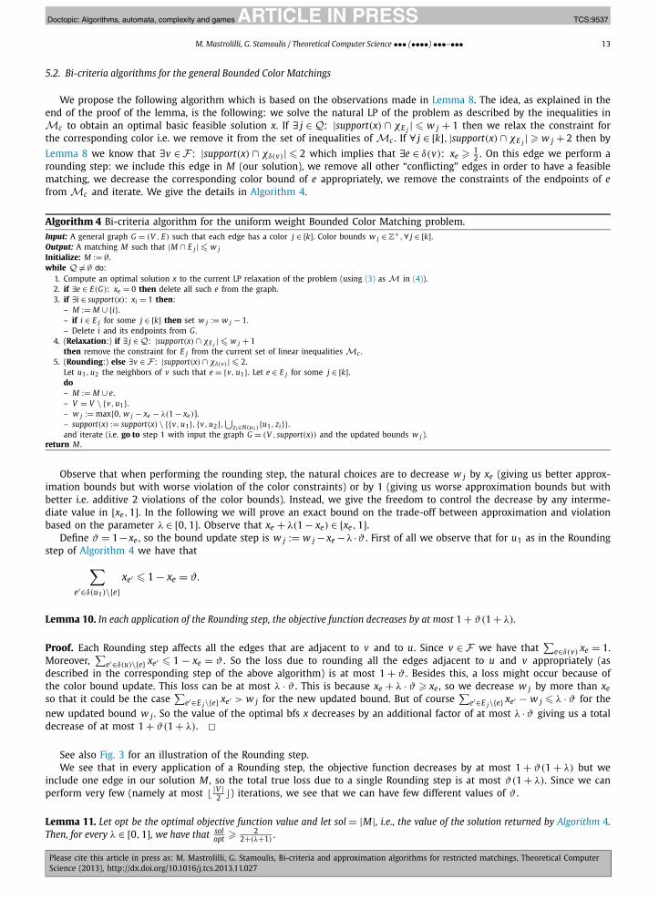
5.2. Bi-criteria algorithms for the general Bounded Color Matchings
We propose the following algorithm which is based on the observations made in Lemma 8. The idea, as explained in theend of the proof of the lemma, is the following: we solve the natural LP of the problem as described by the inequalities inMc to obtain an optimal basic feasible solution x. If ∃ j ∈ Q: |support(x) ∩ χE j | � w j + 1 then we relax the constraint forthe corresponding color i.e. we remove it from the set of inequalities of Mc . If ∀ j ∈ [k], |support(x) ∩ χE j | � w j + 2 then by
Lemma 8 we know that ∃v ∈ F : |support(x) ∩ χδ(v)| � 2 which implies that ∃e ∈ δ(v): xe � 12 . On this edge we perform a
rounding step: we include this edge in M (our solution), we remove all other “conflicting” edges in order to have a feasiblematching, we decrease the corresponding color bound of e appropriately, we remove the constraints of the endpoints of efrom Mc and iterate. We give the details in Algorithm 4.
Algorithm 4 Bi-criteria algorithm for the uniform weight Bounded Color Matching problem.Input: A general graph G = (V , E) such that each edge has a color j ∈ [k]. Color bounds w j ∈ Z+,∀ j ∈ [k].Output: A matching M such that |M ∩ E j | � w j
Initialize: M := ∅.while Q �= ∅ do:
1. Compute an optimal solution x to the current LP relaxation of the problem (using (3) as M in (4)).2. if ∃e ∈ E(G): xe = 0 then delete all such e from the graph.3. if ∃i ∈ support(x): xi = 1 then:
– M := M ∪ {i}.– if i ∈ E j for some j ∈ [k] then set w j := w j − 1.– Delete i and its endpoints from G .
4. (Relaxation:) if ∃ j ∈ Q: |support(x) ∩ χE j | � w j + 1then remove the constraint for E j from the current set of linear inequalities Mc .
5. (Rounding:) else ∃v ∈ F : |support(x) ∩ χδ(v)| � 2.Let u1, u2 the neighbors of v such that e = {v, u1}. Let e ∈ E j for some j ∈ [k].do– M := M ∪ e.– V = V \ {v, u1}.– w j := max{0, w j − xe − λ(1 − xe)}.– support(x) := support(x) \ {{v, u1}, {v, u2},⋃zi∈N(u1){u1, zi}}.and iterate (i.e. go to step 1 with input the graph G = (V , support(x)) and the updated bounds w j ).
return M .
Observe that when performing the rounding step, the natural choices are to decrease w j by xe (giving us better approx-imation bounds but with worse violation of the color constraints) or by 1 (giving us worse approximation bounds but withbetter i.e. additive 2 violations of the color bounds). Instead, we give the freedom to control the decrease by any interme-diate value in [xe,1]. In the following we will prove an exact bound on the trade-off between approximation and violationbased on the parameter λ ∈ [0,1]. Observe that xe + λ(1 − xe) ∈ [xe,1].
Define ϑ = 1− xe , so the bound update step is w j := w j − xe −λ ·ϑ . First of all we observe that for u1 as in the Roundingstep of Algorithm 4 we have that
∑e′∈δ(u1)\{e}
xe′ � 1 − xe = ϑ.
Lemma 10. In each application of the Rounding step, the objective function decreases by at most 1 + ϑ(1 + λ).
Proof. Each Rounding step affects all the edges that are adjacent to v and to u. Since v ∈ F we have that∑
e∈δ(v) xe = 1.Moreover,
∑e′∈δ(u)\{e} xe′ � 1 − xe = ϑ . So the loss due to rounding all the edges adjacent to u and v appropriately (as
described in the corresponding step of the above algorithm) is at most 1 + ϑ . Besides this, a loss might occur because ofthe color bound update. This loss can be at most λ · ϑ . This is because xe + λ · ϑ � xe , so we decrease w j by more than xe
so that it could be the case∑
e′∈E j\{e} xe′ > w j for the new updated bound. But of course∑
e′∈E j\{e} xe′ − w j � λ · ϑ for thenew updated bound w j . So the value of the optimal bfs x decreases by an additional factor of at most λ ·ϑ giving us a totaldecrease of at most 1 + ϑ(1 + λ). �
See also Fig. 3 for an illustration of the Rounding step.We see that in every application of a Rounding step, the objective function decreases by at most 1 + ϑ(1 + λ) but we
include one edge in our solution M , so the total true loss due to a single Rounding step is at most ϑ(1 + λ). Since we canperform very few (namely at most � |V |
2 �) iterations, we see that we can have few different values of ϑ .
Lemma 11. Let opt be the optimal objective function value and let sol = |M|, i.e., the value of the solution returned by Algorithm 4.Then, for every λ ∈ [0,1], we have that sol � 2 .
opt 2+(λ+1)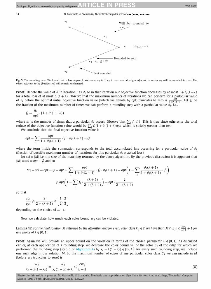
JID:TCS AID:9537 /FLA Doctopic: Algorithms, automata, complexity and games [m3G; v 1.117; Prn:2/12/2013; 15:44] P.14 (1-18)
14 M. Mastrolilli, G. Stamoulis / Theoretical Computer Science ••• (••••) •••–•••
Fig. 3. The rounding case. We know that v has degree 2. We round e1 to 1, e2 to zero and all edges adjacent to vertex u1 will be rounded to zero. Theedges adjacent to u2 (besides e2) will remain unchanged.
Proof. Denote the value of ϑ in iteration i as ϑi so in that iteration our objective function decreases by at most 1+ϑi(1+λ)
for a total loss of at most ϑi(1 + λ). Observe that the maximum number of iterations we can perform for a particular valueof ϑi before the optimal initial objective function value (which we denote by opt) truncates to zero is opt
1+ϑi(1+λ). Let f i be
the fraction of the maximum number of times we can perform a rounding step with a particular value ϑi , i.e.,
f i = ni
opt· (1 + ϑi(1 + λ)
)where ni is the number of times that a particular ϑi occurs. Observe that
∑i f i � 1. This is true since otherwise the total
reduce of the objective function value would be∑
i f i(1 + ϑi(1 + λ))opt which is strictly greater than opt.We conclude that the final objective function value is
opt −∑
i
opt
1 + ϑi(λ + 1)· f i · ϑi(λ + 1) = G
where the term inside the summation corresponds to the total accumulated loss occurring for a particular value of ϑi(fraction of possible maximum number of iterations for this particular ϑi × actual loss).
Let sol = |M| i.e. the size of the matching returned by the above algorithm. By the previous discussion it is apparent that|M| = sol = opt − G and so
|M| = sol = opt − G = opt −∑
i
opt
1 + ϑi(λ + 1)· f i · ϑi(λ + 1) = opt
(1 −
∑i
ϑi(λ + 1)
1 + ϑi(λ + 1)· f i
)
� opt
(1 −
∑i
f i · (λ + 1)
2 + (λ + 1)
)= opt · 2
2 + (λ + 1)
so that
sol
opt� 2
2 + (λ + 1)∈
[1
2,
2
3
]
depending on the choice of λ. �Now we calculate how much each color bound w j can be violated.
Lemma 12. For the final solution M returned by the algorithm and for every color class C j ∈ C we have that |M ∩ E j| � 2w jλ+1 + 1 for
any choice of λ ∈ [0,1].
Proof. Again we will provide an upper bound on the violation in terms of the chosen parameter λ ∈ [0,1]. As discussedearlier, at each application of a rounding step, we decrease the color bound w j of the color C j of the edge for which weperformed the rounding step (step 5 of Algorithm 4) by xe + λ(1 − xe) ∈ [xe,1]. For every such rounding step, we includeone such edge in our solution M . So the maximum number of edges of any particular color class C j we can include in M(before w j truncates to zero) is
w j = w j � 2w j (8)
xe + λ(1 − xe) xe(1 − λ) + λ λ + 1
JID:TCS AID:9537 /FLA Doctopic: Algorithms, automata, complexity and games [m3G; v 1.117; Prn:2/12/2013; 15:44] P.15 (1-18)
M. Mastrolilli, G. Stamoulis / Theoretical Computer Science ••• (••••) •••–••• 15
where the last inequality follows because of the fact that we perform rounding steps at edges with fractional value � 12 .
The extra +1 term in the above formula comes from a possible relaxation step when w j � 1 and there is at most one suchstep per color class. �Corollary 3. For every λ ∈ [0,1], there exists a (( 2
2+(λ+1),0), ( 2
λ+1 ,1)) bi-criteria approximation algorithm for the uniform weightBounded Color Matching problem in general graphs.
Observe that by selecting λ � 12 , we get an approximate solution strictly greater than 4opt
7 0.571 (beating the 0.5
integrality gap) in which each color bound w j is violated by at most an additivew j3 + 1 edge i.e. M has a surplus of at most
w j3 + 1 edges of each color C j .
5.3. A 1/2-approximation algorithm for the uniform weight case
So far, with the exception of the greedy 1/3 algorithm, we have presented bi-criteria algorithms that may potentiallyviolate the color bounds w j . Our main result is that by allowing moderate violation of these color bounds, we can “beat”the integrality gap. The problem is these algorithms fail to achieve the 1/2 integrality gap without violation (the two previousalgorithms give 1/2 approximation on the objective function with at most one extra edge per color). In this subsection wewill show how we can design a 1/2 approximation algorithm for the uniform weight Bounded Color Matching problem ingeneral graphs, showing that the integrality gap is essentially 1/2.
The algorithm again uses the characterization provided by Lemma 8, with the only difference is that we do not performany relaxation step (such a step always result in a color bound violation). Instead, we perform only rounding steps whichare summarized below (the rest of the algorithm is identical with the one of the previous subsection) i.e. the Relaxationstep is replaced by another Rounding step:
• if ∃v ∈ F such that deg(v) = 2, then perform the usual Rounding step (see previous algorithm’s step 5) with parameterλ = 1.
• else ∃C j ∈Q such that
∣∣support(x) ∩ χE j
∣∣ � w j + 1 ⇒ ∃e = {u, v} ∈ C j: xe �w j
w j + 1.
Now, perform a Rounding step for that edge.
The last step is done as follows: Round up xe to 1. Round down to zero all other edges adjacent to vertices u and v (theendpoints of e). Decrease w j by 1 and iterate.
We claim that this simple step result to a 1/2 approximation algorithm for the Bounded Color Matching problem withoutany violation:
Lemma 13. If instead or the Relaxation step (step 4 of Algorithm 4) we perform a Rounding step as described above, then Algorithm 4is a 1/2-approximation algorithm for the BCM problem in uniform weighted graphs without any violation.
Proof. In order to prove the claim of the lemma we will distinguish between the two cases corresponding to the twodifferent rounding steps. In each step, obviously, the gain that we have is 1 (we take one edge in our final solution). Wewill show that in both cases the decrease of the optimal objective function value after the resolution of the LP is at most 2.In conclusion we will show that the gain over loss in each step is at least 1/2, and this will conclude the claim.
To this end, let LP(k) be the optimal objective function value at step k. At this step, we perform one of the two aboverounding steps and resolve the new LP which will have optimal value LP(k +1). The main claim is that LP(k)−LP(k +1) � 2.
If the performed rounding step is done on an edge e because of a vertex v ∈F with degree 2, then the total decrease inthe objective function value in the next iteration is at most
∑e∈δ(v)
xe +∑
e′∈δ(u)\e
xe′ + (1 − xe) � 1 + (1 − xe) + (1 − xe) = 3 − 2xe � 2
where the first term corresponds to the two edges adjacent to v (e will be rounded to one and the other to zero), the secondterm corresponds to the edges (excluding e) adjacent to u that will be rounded to zero, and the third term corresponds toa potential reduce of some other edges of color C j such that e ∈ C j , because of the color bound update step w j = w j − 1.The reason for the last term is the following: color C j of edge e can be (almost) tight, thus if xe is close to 1/2 thenthis leaves us with a surplus of 1 − xe (close to 1/2) of the edges of color C j . So, in the next iteration, the value of therest of the edges of color C j will be reduced by at most 1 − xe but it can be the case that we cannot take advantageof this decrease to increase some other color class. For example, assume that e is blue, wblue = 10 and xe = 1/2. Then
JID:TCS AID:9537 /FLA Doctopic: Algorithms, automata, complexity and games [m3G; v 1.117; Prn:2/12/2013; 15:44] P.16 (1-18)
16 M. Mastrolilli, G. Stamoulis / Theoretical Computer Science ••• (••••) •••–•••
∑e∈Eblue,e′ �=e xe′ = wblue − 1/2 = 9.5 in the worst case. But the update step will reduce wblue by 1 i.e. in the next iteration
wblue = 9 so the new LP solution will have to reduce the value of the blue edges by 1/2 (from 9.5 to 9).Now we consider the case where the rounding step is done because of the presence of a tight color class C j ∈ Q such
that |support(x)∩χE j | = w j + 1. In this case, we know that ∃e ∈ C j: xe � w jw j+1 . This edge will be rounded to one, and some
other appropriate edges will be rounded to zero in such a way to preserve feasibility. Let {u, v} = e as before. Then whenwe round xe to one, we need to round all other edges adjacent to u and v to zero in order to have a feasible matching. Inorder to compute the total decrease � in the LP value by such a step, we first compute what we had before the performedrounding step. Thus, the total decrease of the LP value is at most
� = (1 − xe)︸ ︷︷ ︸decrease on vertex v
+ (1 − xe)︸ ︷︷ ︸decrease on vertex u
+ (1 − xe)︸ ︷︷ ︸color bound update
+ xe = 3 − 2xe
i.e. the first two terms correspond to the loss due to rounding to zero the edges adjacent to u and v , and the third termcorresponds to loss due to color bound update (see the previous case for justification). The fourth term is simply the valueof the edge e. Now, due to the fact that
w jw j+1 � 1
2 , we have that
�� 3 − 2xe � 3 − 2 · w j
w j + 1� 3 − 2 · 1
2= 2.
Observe that w j remains integral in such a case, because it is initially integer and in every step it is reduced exactly by oneunit.
So, in conclusion, in each rounding step, the total accumulated loss is at most two units in the LP value, but the totalgain is exactly one unit (we add one edge in M) proving the claim. �Theorem 4. There exists a 1
2 polynomial time approximation algorithm for the uniform weight Bounded Color Matching problem.
6. Conclusions
In this work, we have presented bi-criteria approximation algorithms for the Bounded Color Matching problem (a.k.a.Restricted Matching problem) that achieve constant approximation guarantee on both criteria of
1. maximizing the objective function value, and2. minimizing the violation of the color constraints bounds.
Our techniques were based on polyhedral characterizations of the natural linear program formulation of the problem(described by the Mc inequalities). This polyhedron has integrality gap 1
2 . We have presented a 12 -approximation algorithm
for the uniform wight case and we have shown how, by allowing a slight violation of the color bound constraints, we candesign approximation algorithms with better than 1
2 guarantee (in the objective function value). Our proposed algorithmin fact is flexible enough to allow any desired guarantee within some given bounds, and provides a trade-off between theapproximability of the objective function value and the violations of the color bounds.
Moreover, for the special case where w j = 1, ∀ j ∈ [k] we have shown how we can obtain an asymptotic approximationguarantee (i.e. approximate the objective function to within arbitrary precision) but at the cost of violating the color boundsw j by at most an additive α − 1 for a given parameter α ∈ Z+ .
Given the limitation of the natural linear program formulation of the problem (captured by its integrality gap), it isnatural to ask if there is another linear program formulation of the problem with better behavior. It is not obvious at all howsuch a linear program might look like (if it exists). But fortunately, there exists machinery from polyhedral theory, called“lift-and-project” method, that allows us to strengthen a particular linear program by adding a set of valid inequalities. Manysuch lift-and-project methods have been proposed so far for example by Sherali and Adams [50], by Lovász and Schrijver[38], by Balas, Ceria and Cornuéjols [1,2] and by Lasserre [34,33].
Let P0 = {x ∈ {0,1}n: Ax � β}, A ∈Rm×n, β ∈ Rm , be an initial polyhedron in the nth dimensional space. All the previoustechniques follow the same pattern: they operate in rounds, and in each round a specific set of linear (Sherali–Adams andBalas, Ceria and Cornuéjols) or semi-definite (in the case of Lovász and Schrijver and Lasserre) inequalities are added. Thuswe obtain a hierarchy of tighter formulations Kn ⊆ Kn−1 ⊆ · · · ⊆ K1 of an initial relaxation of an integral polyhedron I whereK1 is just the relaxation of P0. The important features, common in all these hierarchies is that we can efficiently optimizeany linear (or semi-definite) objective function over Kt for any fixed t and, moreover, after n at most steps, we will arriveat an exact formulation of the convex hull of all the integral points if I , i.e., Kn = P0.
All the previous hierarchies (except the Balas, Ceria and Cornuéjols) are placed in a common framework in the workof Monique Laurent [36] who proves, among many other things, that the Sherali–Adams hierarchy is incomparable thanthe Lovász–Schrijver hierarchy but stronger that Lovász–Schrijver with linear lifting inequalities. Moreover, it is shown thatthe Lasserre hierarchy is stronger than any of the previous. It would be a very interesting research direction to investigatehow the integrality gap changes after the application of any of these hierarchies. And, moreover, the possibility to obtain a
JID:TCS AID:9537 /FLA Doctopic: Algorithms, automata, complexity and games [m3G; v 1.117; Prn:2/12/2013; 15:44] P.17 (1-18)
M. Mastrolilli, G. Stamoulis / Theoretical Computer Science ••• (••••) •••–••• 17
tighter description of the convex hull of the integral points of the bounded matching polyhedron, leaves open the possibilityof designing approximation algorithms with better performance guarantee.
Acknowledgements
We would like to thank Christos Nomikos for introducing us to the problem and for many valuable and pleasant dis-cussions. Moreover, we would like to sincerely thank the reviewers of the 2nd International Symposium on CombinatorialOptimization (ISCO ’12) for carefully reading the preliminary version of this work and for many helpful suggestions andcomments that improved the presentation of this work.
References
[1] E. Balas, S. Ceria, G. Cornuéjols, A lift-and-project cutting plane algorithm for mixed 0–1 programs, Math. Program. 58 (1993) 295–324.[2] E. Balas, S. Ceria, G. Cornuéjols, Solving mixed 0–1 programs by a lift-and-project method, in: V. Ramachandran (Ed.), SODA 1993, ACM/SIAM, 1993,
pp. 232–242.[3] E. Bampas, A. Pagourtzis, K. Potika, An experimental study of maximum profit wavelength assignment in WDM rings, Networks 57 (3) (2011) 285–293.[4] N. Bansal, R. Khandekar, V. Nagarajan, Additive guarantees for degree-bounded directed network design, SIAM J. Comput. 39 (4) (2009) 1413–1431.[5] C. Berge, Sur le couplage maximum d’un graphe, C. R. Acad. Sci. Paris 247 (1958) 258–259.[6] A. Berger, V. Bonifaci, F. Grandoni, G. Schäfer, Budgeted matching and budgeted matroid intersection via the gasoline puzzle, in: A. Lodi, A. Panconesi,
G. Rinaldi (Eds.), IPCO 2008, in: Lecture Notes in Computer Science, vol. 5035, Springer, 2008, pp. 273–287.[7] A. Berger, V. Bonifaci, F. Grandoni, G. Schäfer, Budgeted matching and budgeted matroid intersection via the gasoline puzzle, Math. Program. 128 (1–2)
(2011) 355–372.[8] I. Caragiannis, Wavelength management in WDM rings to maximize the number of connections, in: W. Thomas, P. Weil (Eds.), STACS 2007, in: Lecture
Notes in Computer Science, vol. 4393, Springer, 2007, pp. 61–72.[9] I. Caragiannis, Wavelength management in WDM rings to maximize the number of connections, SIAM J. Discrete Math. 23 (2) (2009) 959–978.
[10] C. Carathéodory, Über den Variabilitätsbereich der Fourierschen Konstanten von positiven harmonischen Funktionen, Rend. Circ. Mat. Palermo 32 (1911)193–217.
[11] F. Carrabs, R. Cerulli, M. Gentili, The labeled maximum matching problem, Comput. Oper. Res. 36 (6) (2009) 1859–1871.[12] C. Chekuri, J. Vondrák, R. Zenklusen, Dependent randomized rounding via exchange properties of combinatorial structures, in: FOCS 2010, IEEE Com-
puter Society, 2010, pp. 575–584.[13] C. Chekuri, J. Vondrák, R. Zenklusen, Multi-budgeted matchings and matroid intersection via dependent rounding, in: D. Randall (Ed.), SODA 2011,
SIAM, 2011, pp. 1080–1097.[14] W.J. Cook, W.H. Cunningham, W.R. Pulleyblank, A. Schrijver, Combinatorial Optimization, John Wiley & Sons, 2011.[15] W. Cunningham, A. Marsh, A primal algorithm for optimum matching, Math. Program. Stud. 29 (1978) 50–72.[16] J. Edmonds, Maximum matching and a polyhedron with 0,1 vertices, J. Res. Natl. Bur. Stand. 69B (1965) 125–130.[17] J. Edmonds, Paths, trees, and flowers, Can. J. Math. 17 (1965) 449–467.[18] S. Even, O. Kariv, An O (n2.5) algorithm for maximum matching in general graphs, in: FOCS 1975, IEEE Computer Society, 1975, pp. 100–112.[19] H.N. Gabow, Scaling algorithms for network problems, in: FOCS, IEEE Computer Society, 1983, pp. 248–257.[20] H.N. Gabow, Scaling algorithms for network problems, J. Comput. Syst. Sci. 31 (2) (1985) 148–168.[21] H.N. Gabow, R.E. Tarjan, Faster scaling algorithms for general graph-matching problems, J. ACM 38 (4) (1991) 815–853.[22] M.R. Garey, D.S. Johnson, Computers and Intractability: A Guide to the Theory of NP-Completeness, W.H. Freeman, 1979.[23] F. Grandoni, R. Ravi, M. Singh, Iterative rounding for multi-objective optimization problems, in: A. Fiat, P. Sanders (Eds.), ESA 2009, in: Lecture Notes
in Computer Science, vol. 5757, Springer, 2009, pp. 95–106.[24] F. Grandoni, R. Zenklusen, Approximation schemes for multi-budgeted independence systems, in: M. de Berg, U. Meyer (Eds.), ESA (1) 2010, in: Lecture
Notes in Computer Science, vol. 6346, Springer, 2010, pp. 536–548.[25] F. Grandoni, R. Zenklusen, Optimization with more than one budget, arXiv:1002.2147, 2010.[26] N.J.A. Harvey, Algebraic structures and algorithms for matching and matroid problems, in: FOCS, IEEE Computer Society, 2006, pp. 531–542.[27] N.J.A. Harvey, Algebraic algorithms for matching and matroid problems, SIAM J. Comput. 39 (2) (2009) 679–702.[28] J.E. Hopcroft, R.M. Karp, A n5/2 algorithm for maximum matchings in bipartite graphs, in: SWAT (FOCS 1971), IEEE Computer Society, 1971,
pp. 122–125.[29] J.E. Hopcroft, R.M. Karp, An n5/2 algorithm for maximum matchings in bipartite graphs, SIAM J. Comput. 2 (4) (1973) 225–231.[30] A. Itai, M. Rodeh, Some matching problems, in: A. Salomaa, M. Steinby (Eds.), ICALP 1977, in: Lecture Notes in Computer Science, vol. 52, Springer,
1977, pp. 258–268.[31] A. Itai, M. Rodeh, S.L. Tanimoto, Some matching problems for bipartite graphs, J. ACM 25 (4) (1978) 517–525.[32] H.W. Kuhn, The Hungarian method for the assignment problem, Nav. Res. Logist. Q. 2 (1955) 83–97.[33] J.B. Lasserre, Global optimization with polynomials and the problem of moments, SIAM J. Optim. 11 (3) (2001) 796–817.[34] J.B. Lasserre, An explicit equivalent positive semidefinite program for nonlinear 0–1 programs, SIAM J. Optim. 12 (3) (2002) 756–769.[35] L.C. Lau, R. Ravi, M. Singh, Iterative Methods in Combinatorial Optimization, Cambridge University Press, 2011.[36] M. Laurent, A comparison of the Sherali–Adams, Lovász–Schrijver, and Lasserre relaxations for 0–1 programming, Math. Oper. Res. 28 (3) (2003)
470–496.[37] L. Lovász, M. Plummer, Matching Theory, North-Holland, 1986.[38] L. Lovász, A. Schrijver, Cones of matrices and set-functions and 0–1 optimization, SIAM J. Optim. 1 (1991) 166–190.[39] J. Mestre, Greedy in approximation algorithms, in: Y. Azar, T. Erlebach (Eds.), ESA, 2006, pp. 528–539.[40] S. Micali, V.V. Vazirani, An O (
√|V ||E|) algorithm for finding maximum matching in general graphs, in: FOCS 1980, IEEE Computer Society, 1980,pp. 17–27.
[41] J. Monnot, The labeled perfect matching in bipartite graphs, Inf. Process. Lett. 96 (3) (2005) 81–88.[42] J. Monnot, On complexity and approximability of the labeled maximum/perfect matching problems, in: X. Deng, D.-Z. Du (Eds.), ISAAC 2005, in: Lecture
Notes in Computer Science, vol. 3827, Springer, 2005, pp. 934–943.[43] M. Mucha, P. Sankowski, Maximum matchings via Gaussian elimination, in: FOCS 2004, IEEE Computer Society, 2004, pp. 248–255.[44] C. Nomikos, A. Pagourtzis, S. Zachos, Minimizing request blocking in all-optical rings, in: IEEE INFOCOM, 2003.[45] C. Nomikos, A. Pagourtzis, S. Zachos, Randomized and approximation algorithms for blue–red matching, in: L. Kucera, A. Kucera (Eds.), MFCS, 2007,
pp. 715–725.

JID:TCS AID:9537 /FLA Doctopic: Algorithms, automata, complexity and games [m3G; v 1.117; Prn:2/12/2013; 15:44] P.18 (1-18)
18 M. Mastrolilli, G. Stamoulis / Theoretical Computer Science ••• (••••) •••–•••
[46] C.H. Papadimitriou, M. Yannakakis, The complexity of restricted spanning tree problems, J. ACM 29 (2) (1982) 285–309.[47] M.O. Rabin, V.V. Vazirani, Maximum matchings in general graphs through randomization, J. Algorithms 10 (4) (1989) 557–567.[48] A. Schrijver, Theory of Linear and Integer Programming, John Wiley & Sons, 1998.[49] A. Schrijver, Combinatorial Optimization: Polyhedra and Efficiency, Springer, 2003.[50] H.D. Sherali, W.P. Adams, A hierarchy of relaxations between the continuous and convex hull representations for zero–one programming problems,
SIAM J. Discrete Math. 3 (3) (1990) 411–430.[51] M. Singh, Iterative methods in combinatorial optimization, PhD thesis, Carnegie Mellon University, 2008.[52] R. Yuster, Almost exact matchings, in: M. Charikar, K. Jansen, O. Reingold, J.D.P. Rolim (Eds.), APPROX-RANDOM 2007, in: Lecture Notes in Computer
Science, vol. 4627, Springer, 2007, pp. 286–295.[53] R. Yuster, Almost exact matchings, Algorithmica 63 (1–2) (2012) 39–50.


![Analysis of Stable Matchings in R: Package matchingMarkets · Analysis of Stable Matchings in R: ... 4 Analysis of Stable Matchings in R: Package matchingMarkets ... G = 1[V G 0]](https://img.pdfslide.net/doc/110x75/5b3cc11f7f8b9a9a098b5ae0/analysis-of-stable-matchings-in-r-package-matchingmarkets-analysis-of-stable.jpg)