Embed Size (px)
Citation preview

BIG DATAALGORITHMS

GOOGLE TREND

BIG DATA
everyone talks about it,
nobody really knows how to do it,
everyone thinks everyone else is doing it,
so everyone claims they are doing it...


IS THERE ANYTHING FUNDAMENTALLY NEW?
• Massive Data vs Big Data
• The 3 V’s
• Volume• Velocity• Variety

BIG DATA ECOSYSTEM

BIG DATA APPLICATIONS
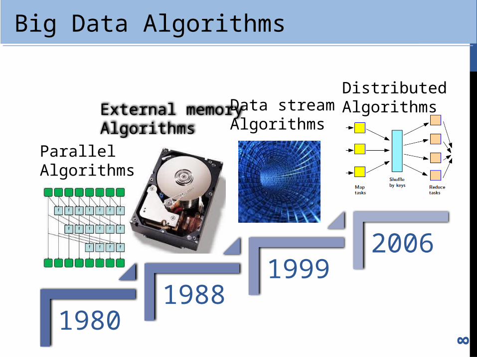
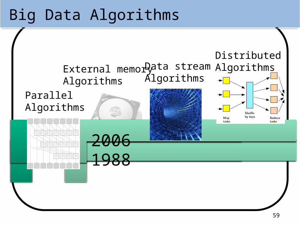
Big Data Algorithms
8
19801988
19992006
External memoryAlgorithms
Data streamAlgorithms
DistributedAlgorithms
ParallelAlgorithms

COMPUTATIONAL MODELS FOR BIG DATA
All models are wrong,But some are useful.
George E. P. Box
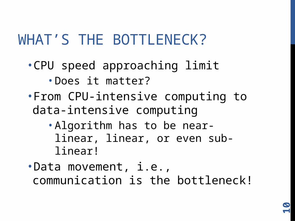
WHAT’S THE BOTTLENECK?
• CPU speed approaching limit• Does it matter?
• From CPU-intensive computing to data-intensive computing
• Algorithm has to be near-linear, linear, or even sub-linear!
• Data movement, i.e., communication is the bottleneck!
10
11
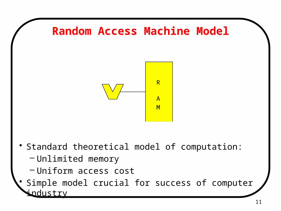
Random Access Machine Model
• Standard theoretical model of computation:– Unlimited memory– Uniform access cost
• Simple model crucial for success of computer industry
R
A
M
12
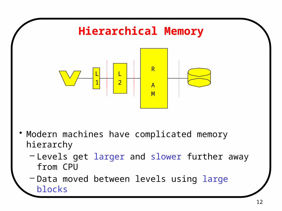
Hierarchical Memory
• Modern machines have complicated memory hierarchy– Levels get larger and slower further away from CPU– Data moved between levels using large blocks
L
1
L
2
R
A
M
13
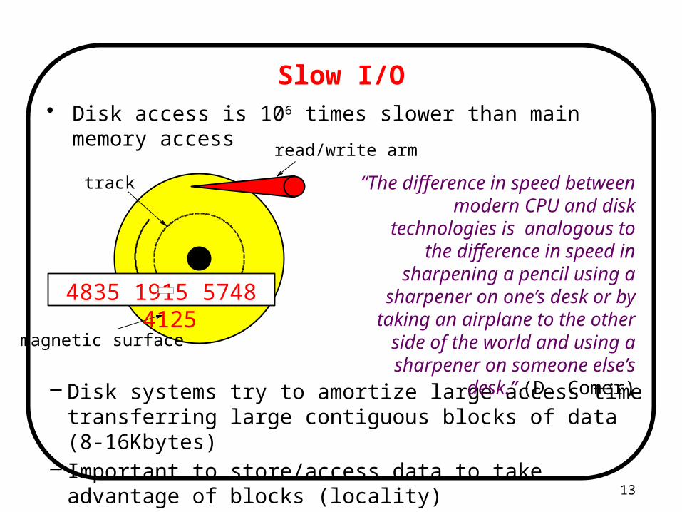
Slow I/O
– Disk systems try to amortize large access time transferring large contiguous blocks of data (8-16Kbytes)
– Important to store/access data to take advantage of blocks (locality)
• Disk access is 106 times slower than main memory access
track
magnetic surface
read/write arm
“The difference in speed between modern CPU and disk
technologies is analogous to the difference in speed in sharpening
a pencil using a sharpener on one’s desk or by taking an
airplane to the other side of the world and using a sharpener on
someone else’s desk.” (D. Comer)
4835 1915 5748 4125
14
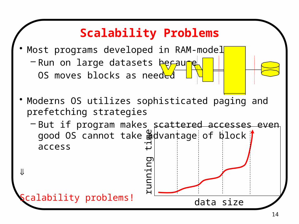
Scalability Problems• Most programs developed in RAM-model
– Run on large datasets because
OS moves blocks as needed
• Moderns OS utilizes sophisticated paging and prefetching strategies– But if program makes scattered accesses even good OS cannot
take advantage of block access
Scalability problems!
data size
runn
ing
tim
e
15
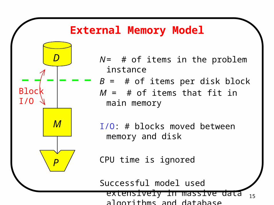
N = # of items in the problem instance
B = # of items per disk block
M = # of items that fit in main memory
I/O: # blocks moved between memory and disk
CPU time is ignored
Successful model used extensively in massive data algorithms and database communities
D
P
M
Block I/O
External Memory Model
16
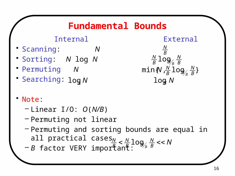
Fundamental Bounds Internal External
• Scanning: N• Sorting: N log N• Permuting • Searching:
• Note:– Linear I/O: O(N/B)– Permuting not linear– Permuting and sorting bounds are equal in all practical cases– B factor VERY important:
NBlog
BN
BN
BMlog
BN
NBN
BN
BN
BM log
}log,min{BN
BN
BMNN
N2log
17
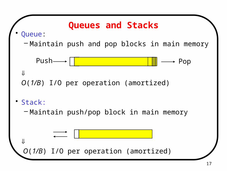
Queues and Stacks• Queue:
– Maintain push and pop blocks in main memory
O(1/B) I/O per operation (amortized)
• Stack:– Maintain push/pop block in main memory
O(1/B) I/O per operation (amortized)
Push Pop
18
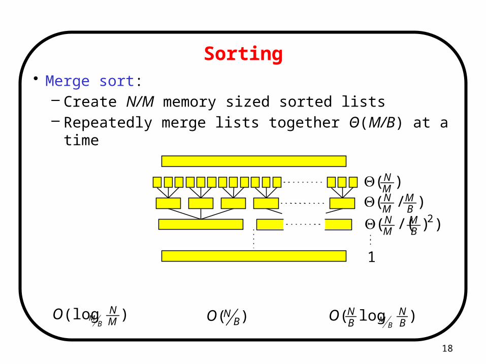
Sorting• Merge sort:
– Create N/M memory sized sorted lists– Repeatedly merge lists together Θ(M/B) at a time
phases using I/Os each I/Os)( BNO)(log
MN
BMO )log(
BN
BN
BMO
)(MN
)/(BM
MN
))/(( 2BM
MN
1
19
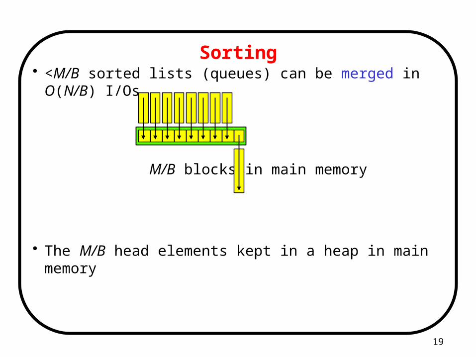
Sorting• <M/B sorted lists (queues) can be merged in O(N/B) I/Os
M/B blocks in main memory
• The M/B head elements kept in a heap in main memory
20
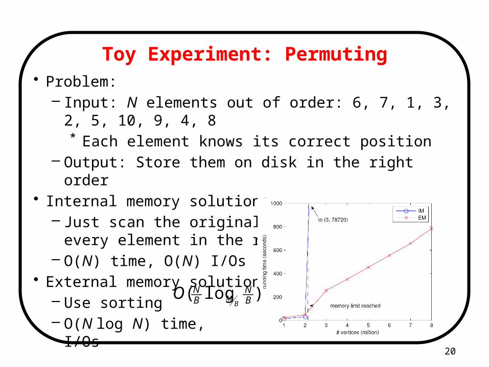
Toy Experiment: Permuting• Problem:
– Input: N elements out of order: 6, 7, 1, 3, 2, 5, 10, 9, 4, 8* Each element knows its correct position
– Output: Store them on disk in the right order• Internal memory solution:
– Just scan the original sequence and move every element in the right place!
– O(N) time, O(N) I/Os• External memory solution:
– Use sorting– O(N log N) time, I/Os)log( B
NBN
BMO

21
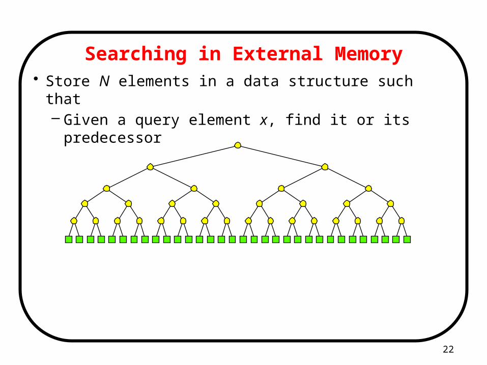
Searching in External Memory• Store N elements in a data structure such that
– Given a query element x, find it or its predecessor
22
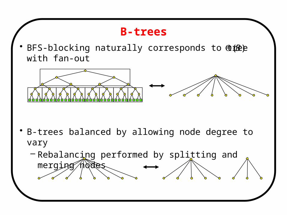
B-trees• BFS-blocking naturally corresponds to tree with fan-out
• B-trees balanced by allowing node degree to vary– Rebalancing performed by splitting and merging nodes
)(B
• (a,b)-tree uses linear space and has heightChoosing a,b = each node/leaf stored in one disk blockO( /N B) space and query
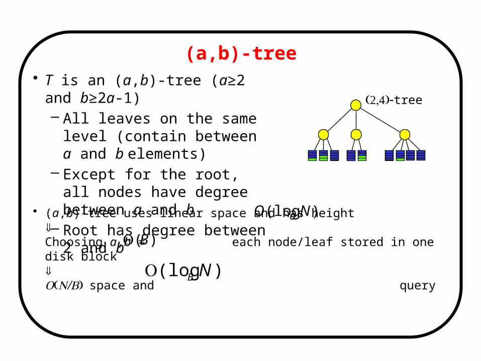
(a,b)-tree• T is an (a,b)-tree (a≥2 and b≥2a-1)
– All leaves on the same level (contain between a and b elements)
– Except for the root, all nodes have degree between a and b
– Root has degree between 2 and b
)(log NO a
)(log NB
)(B
(2,4)-tree
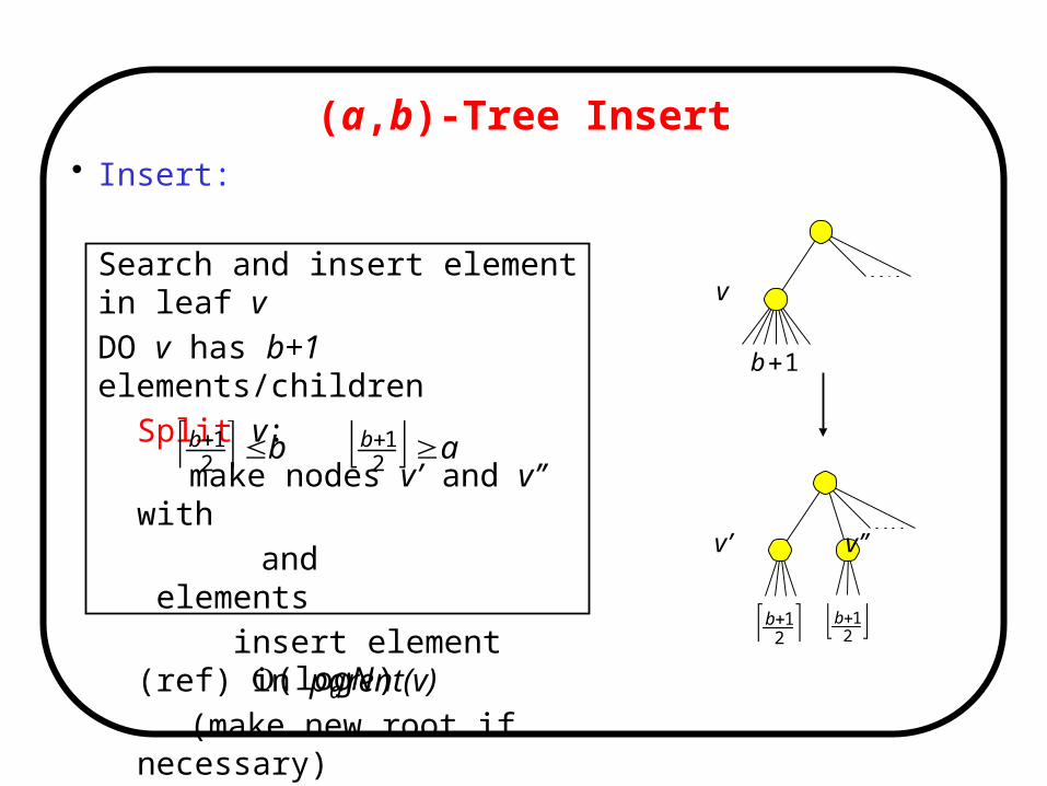
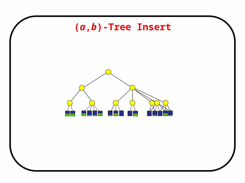
(a,b)-Tree Insert• Insert:
Search and insert element in leaf v
DO v has b+1 elements/children
Split v:
make nodes v’ and v’’ with
and elements
insert element (ref) in parent(v)
(make new root if necessary)
v=parent(v)
• Insert touch nodes
bb 2
1 ab 2
1
)(log Na
v
v’ v’’
21b 2
1b
1b
(a,b)-Tree Insert
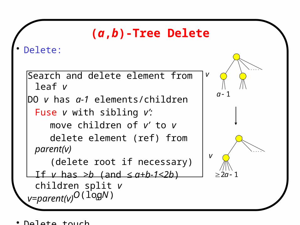
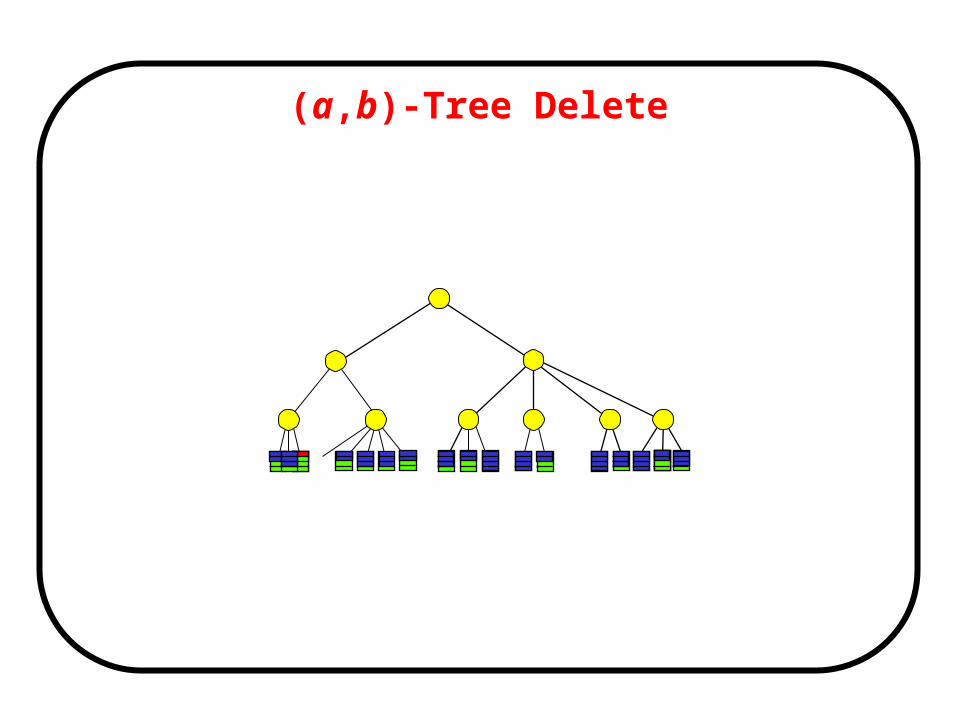
(a,b)-Tree Delete• Delete:
Search and delete element from leaf v
DO v has a-1 elements/children
Fuse v with sibling v’:
move children of v’ to v
delete element (ref) from parent(v)
(delete root if necessary)
If v has >b (and ≤ a+b-1<2b) children split v
v=parent(v)
• Delete touch nodes )(log NO a
v
v
1a
12 a
(a,b)-Tree Delete
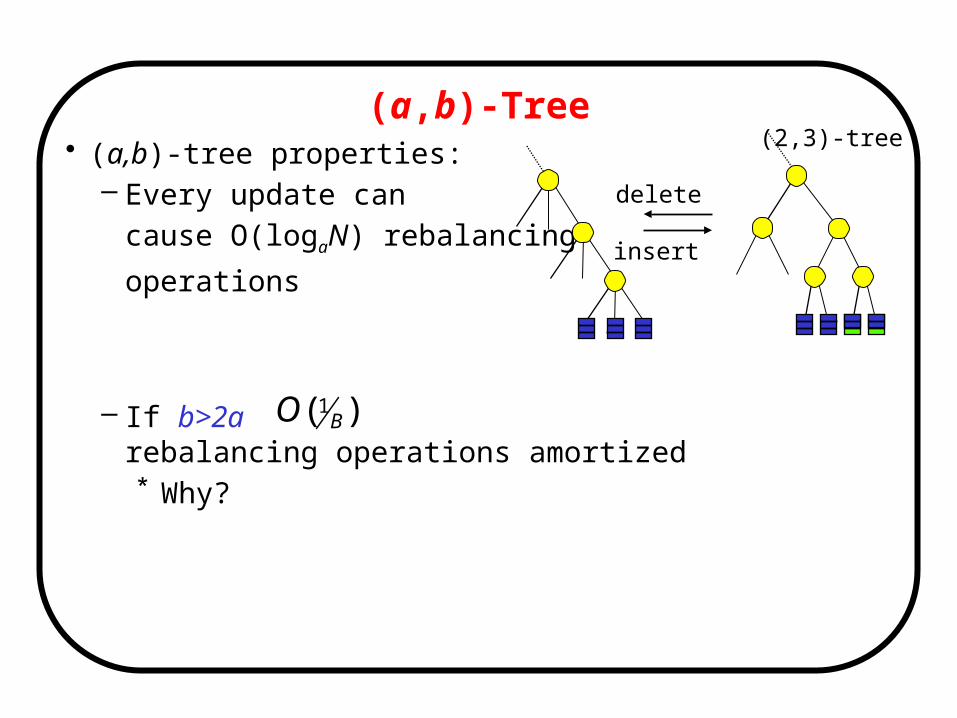
• (a,b)-tree properties:– Every update can
cause O(logaN) rebalancing
operations
– If b>2a rebalancing operations amortized* Why?
(a,b)-Tree
)( 1BO
delete
insert
(2,3)-tree
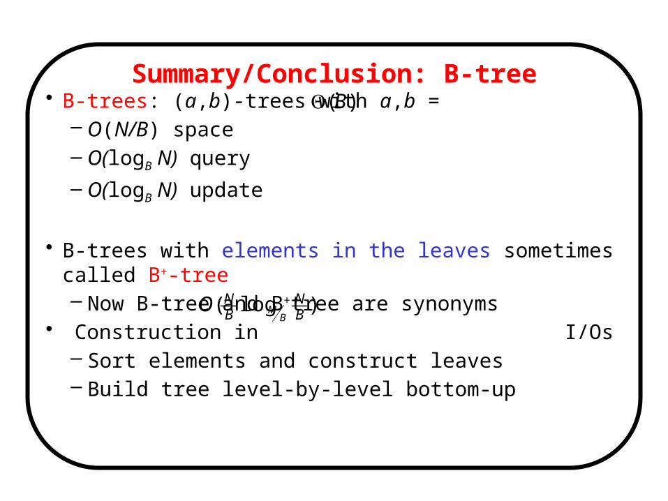
Summary/Conclusion: B-tree• B-trees: (a,b)-trees with a,b =
– O(N/B) space– O(logB N) query
– O(logB N) update
• B-trees with elements in the leaves sometimes called B+-tree– Now B-tree and B+tree are synonyms
• Construction in I/Os– Sort elements and construct leaves– Build tree level-by-level bottom-up
)(B
)log(BN
BN
BMO
Basic Structures: I/O-Efficient Priority Queue
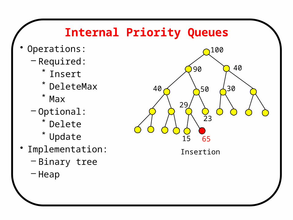
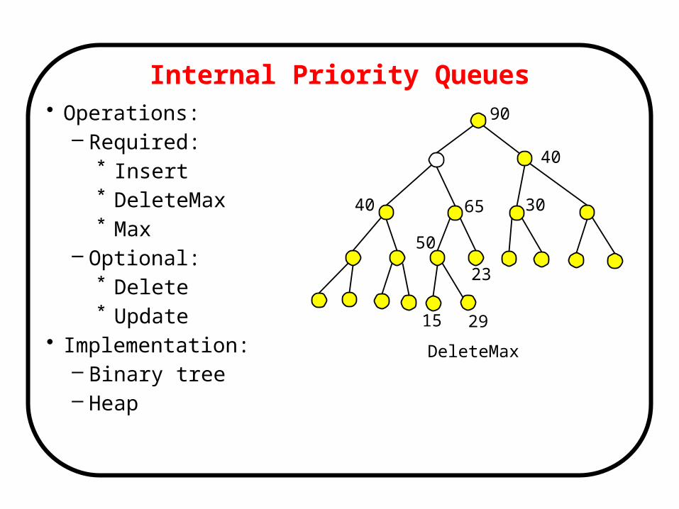
Internal Priority Queues• Operations:
– Required:* Insert* DeleteMax* Max
– Optional:* Delete* Update
• Implementation:– Binary tree– Heap
100
90 40
50 30
29
15
40
23
65
Insertion
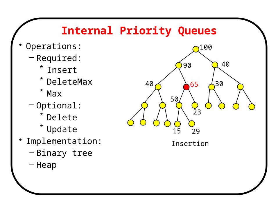
Internal Priority Queues• Operations:
– Required:* Insert* DeleteMax* Max
– Optional:* Delete* Update
• Implementation:– Binary tree– Heap
100
90 40
65 30
50
15
40
23
29
Insertion

Internal Priority Queues• Operations:
– Required:* Insert* DeleteMax* Max
– Optional:* Delete* Update
• Implementation:– Binary tree– Heap
90 40
65 30
50
15
40
23
29
DeleteMax
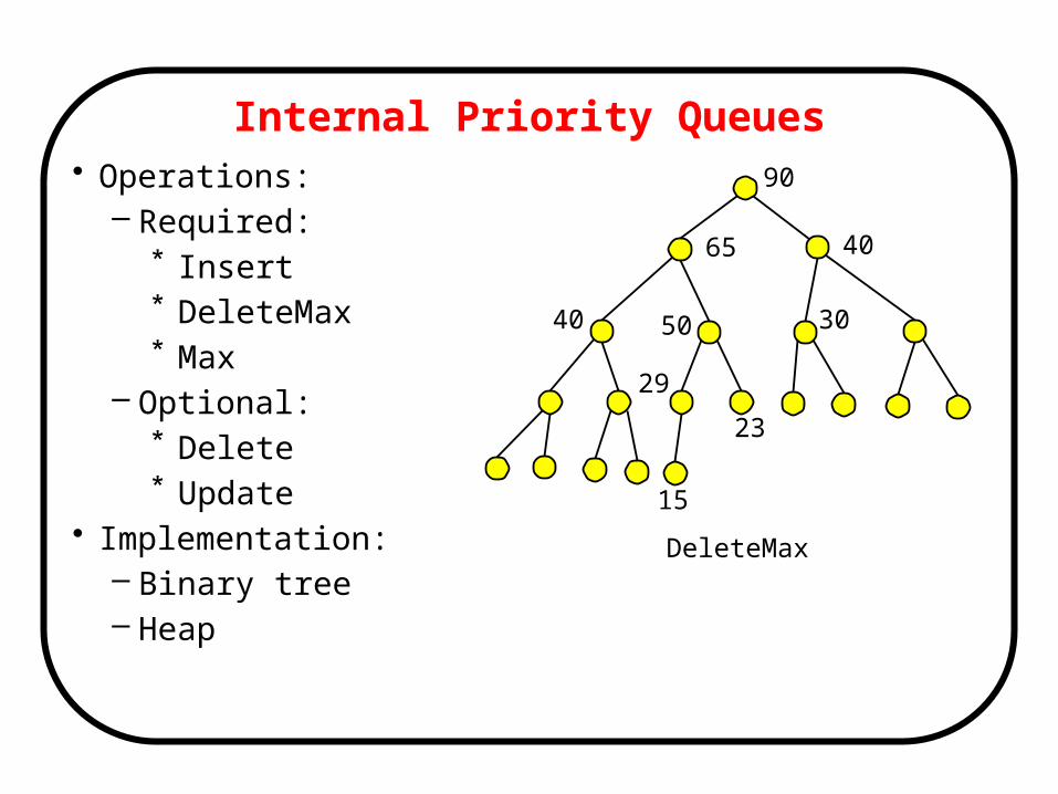
Internal Priority Queues• Operations:
– Required:* Insert* DeleteMax* Max
– Optional:* Delete* Update
• Implementation:– Binary tree– Heap
40
65 30
50
15
40
23
29
DeleteMax
90
Internal Priority Queues• Operations:
– Required:* Insert* DeleteMax* Max
– Optional:* Delete* Update
• Implementation:– Binary tree– Heap
4065
3050
15
40
23
29
DeleteMax
90

How to Make the Heap I/O-Efficient
I/O Technique 1: Make it many-way
I/O Technique 2: Buffering!
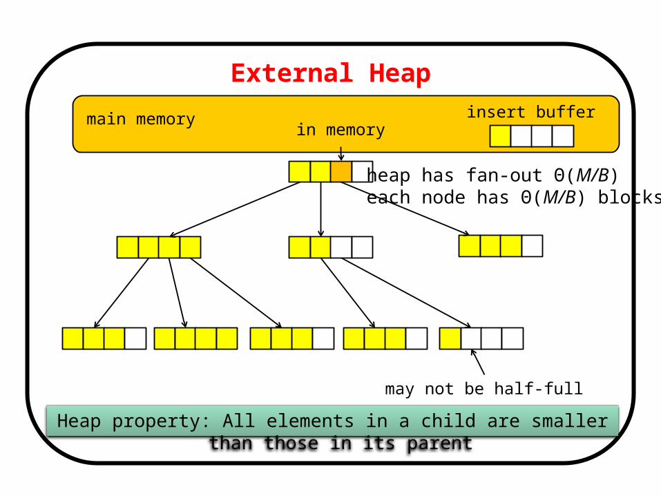
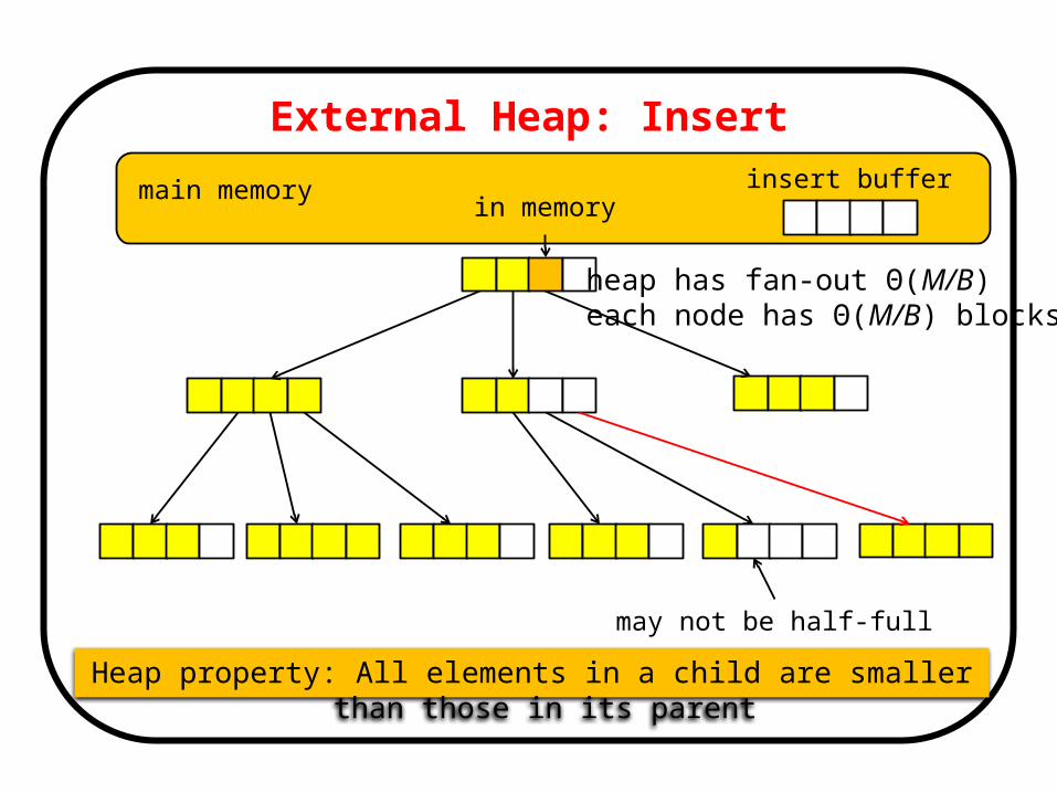
External Heap
main memory
may not be half-full
Heap property: All elements in a child are smaller than those in its parent
insert buffer
heap has fan-out Θ(M/B) each node has Θ(M/B) blocks
in memory
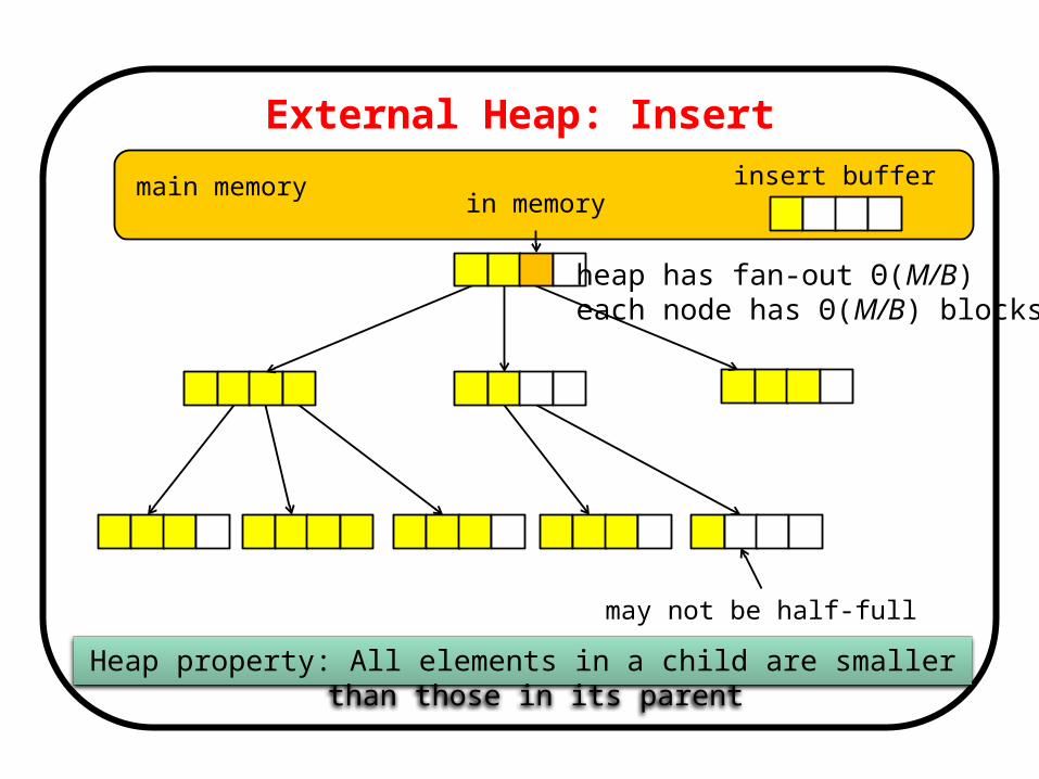
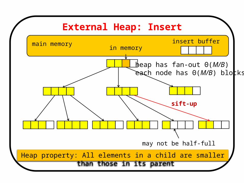
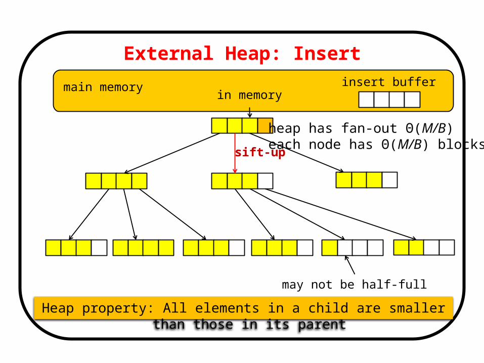
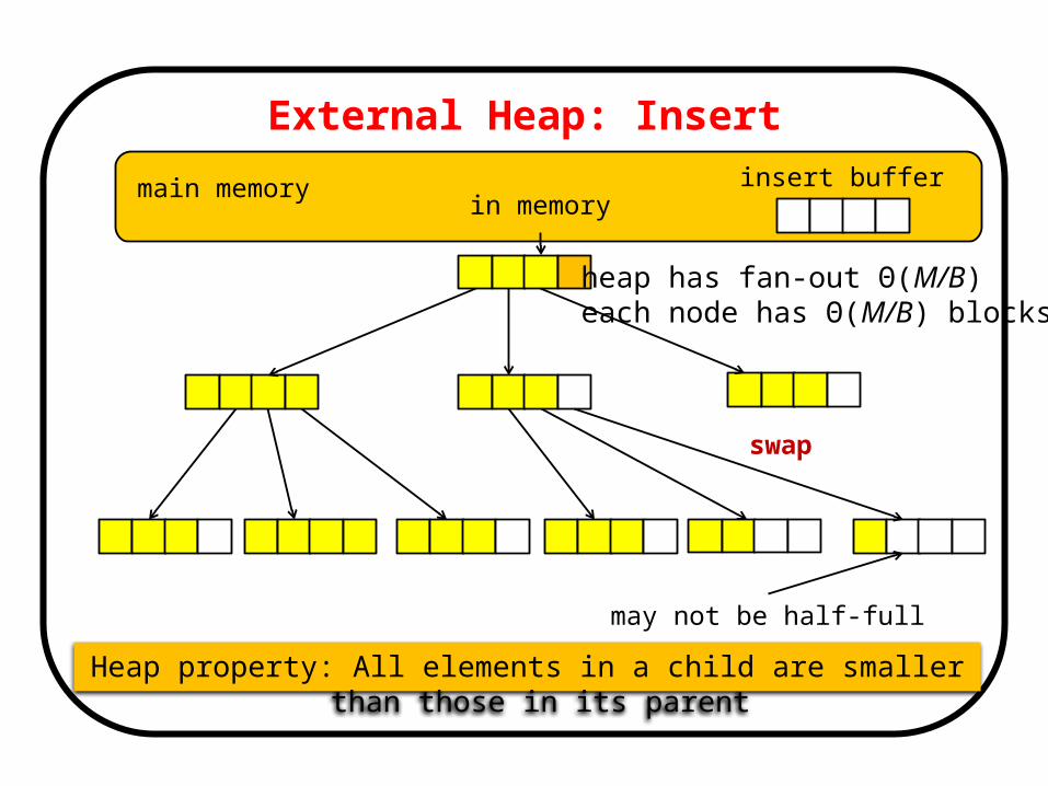
External Heap: Insert
main memory
may not be half-full
Heap property: All elements in a child are smaller than those in its parent
insert buffer
heap has fan-out Θ(M/B) each node has Θ(M/B) blocks
in memory
External Heap: Insert
main memory
may not be half-full
Heap property: All elements in a child are smaller than those in its parent
insert buffer
heap has fan-out Θ(M/B) each node has Θ(M/B) blocks
in memory
External Heap: Insert
main memory
may not be half-full
Heap property: All elements in a child are smaller than those in its parent
insert buffer
heap has fan-out Θ(M/B) each node has Θ(M/B) blocks
in memory
sift-up
External Heap: Insert
main memory
may not be half-full
Heap property: All elements in a child are smaller than those in its parent
insert buffer
heap has fan-out Θ(M/B) each node has Θ(M/B) blocks
in memory
sift-up
External Heap: Insert
main memory
may not be half-full
Heap property: All elements in a child are smaller than those in its parent
insert buffer
heap has fan-out Θ(M/B) each node has Θ(M/B) blocks
in memory
swap
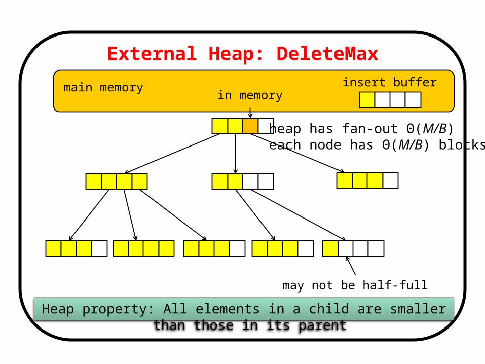
External Heap: DeleteMax
main memory
may not be half-full
Heap property: All elements in a child are smaller than those in its parent
insert buffer
heap has fan-out Θ(M/B) each node has Θ(M/B) blocks
in memory

External Heap: DeleteMax
main memory
may not be half-full
Heap property: All elements in a child are smaller than those in its parent
insert buffer
heap has fan-out Θ(M/B) each node has Θ(M/B) blocks
in memory
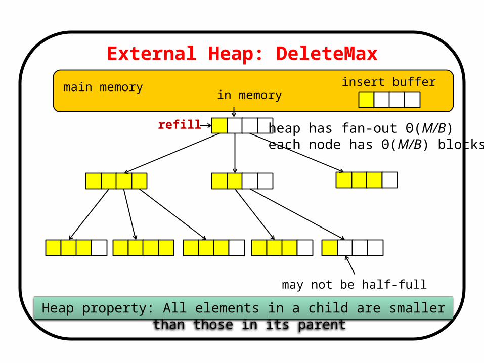
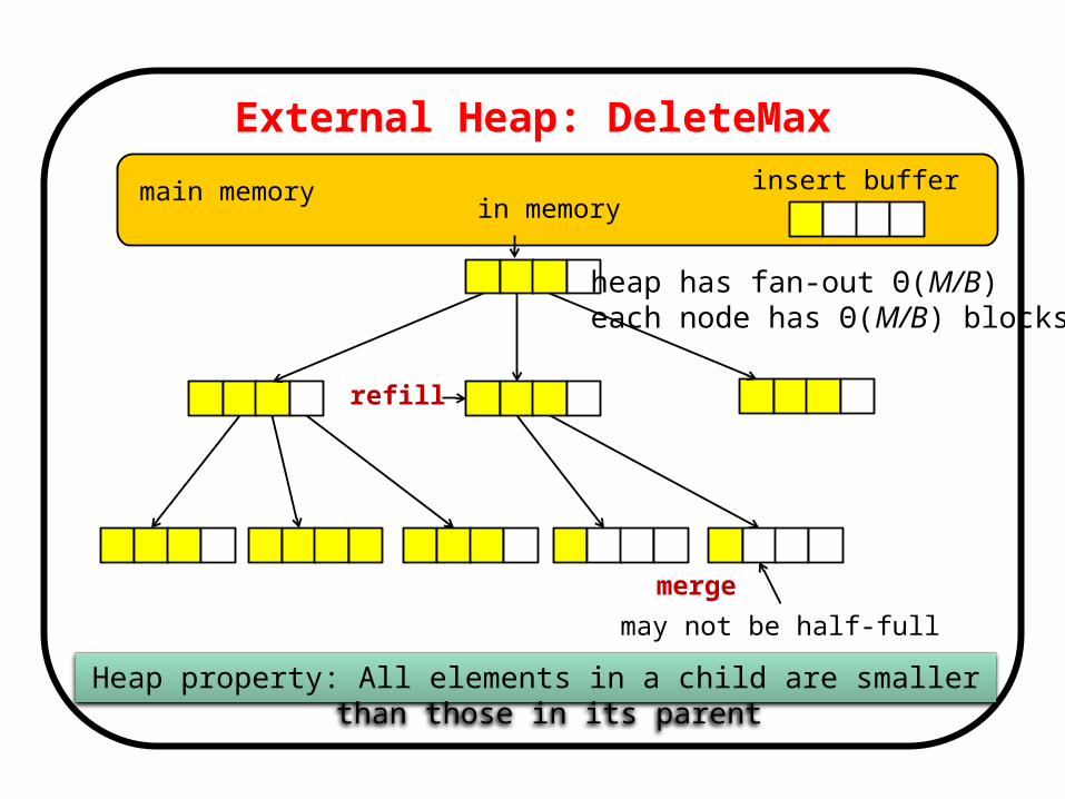
External Heap: DeleteMax
main memory
may not be half-full
Heap property: All elements in a child are smaller than those in its parent
insert buffer
heap has fan-out Θ(M/B) each node has Θ(M/B) blocks
in memory
refill
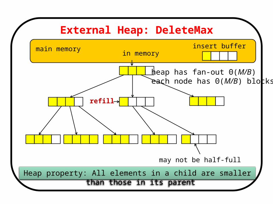
External Heap: DeleteMax
main memory
may not be half-full
Heap property: All elements in a child are smaller than those in its parent
insert buffer
heap has fan-out Θ(M/B) each node has Θ(M/B) blocks
in memory
refill
External Heap: DeleteMax
main memory
may not be half-full
Heap property: All elements in a child are smaller than those in its parent
insert buffer
heap has fan-out Θ(M/B) each node has Θ(M/B) blocks
in memory
refill
merge
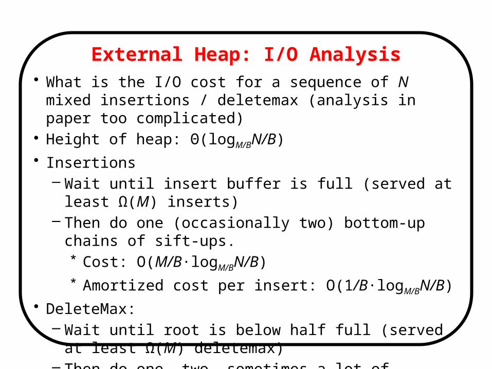
External Heap: I/O Analysis• What is the I/O cost for a sequence of N mixed insertions /
deletemax (analysis in paper too complicated)• Height of heap: Θ(logM/BN/B)
• Insertions– Wait until insert buffer is full (served at least Ω(M) inserts)– Then do one (occasionally two) bottom-up chains of sift-ups.
* Cost: O(M/B∙logM/BN/B)
* Amortized cost per insert: O(1/B∙logM/BN/B)
• DeleteMax:– Wait until root is below half full (served at least Ω(M)
deletemax)– Then do one, two, sometimes a lot of refills… dead– Do one sift-up: this is easy
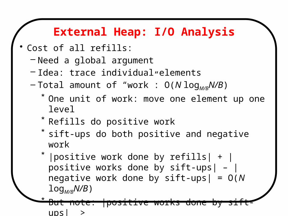
External Heap: I/O Analysis• Cost of all refills:
– Need a global argument– Idea: trace individual elements– Total amount of “work”: O(N logM/BN/B)
* One unit of work: move one element up one level* Refills do positive work* sift-ups do both positive and negative work* |positive work done by refills| + |positive works done by sift-
ups| – |negative work done by sift-ups| = O(N logM/BN/B)
* But note: |positive works done by sift-ups| >|negative work done by sift-ups|
* So, |positive work done by refills| = O(N logM/BN/B)
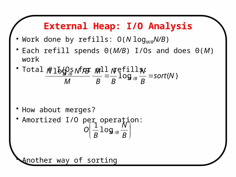
External Heap: I/O Analysis• Work done by refills: O(N logM/BN/B)
• Each refill spends Θ(M/B) I/Os and does Θ(M) work• Total # I/Os for all refills:
• How about merges?• Amortized I/O per operation:
• Another way of sorting
)(log/log
// Nsort
B
N
B
N
B
M
M
BNNBM
BM
B
N
BO BM /log
1
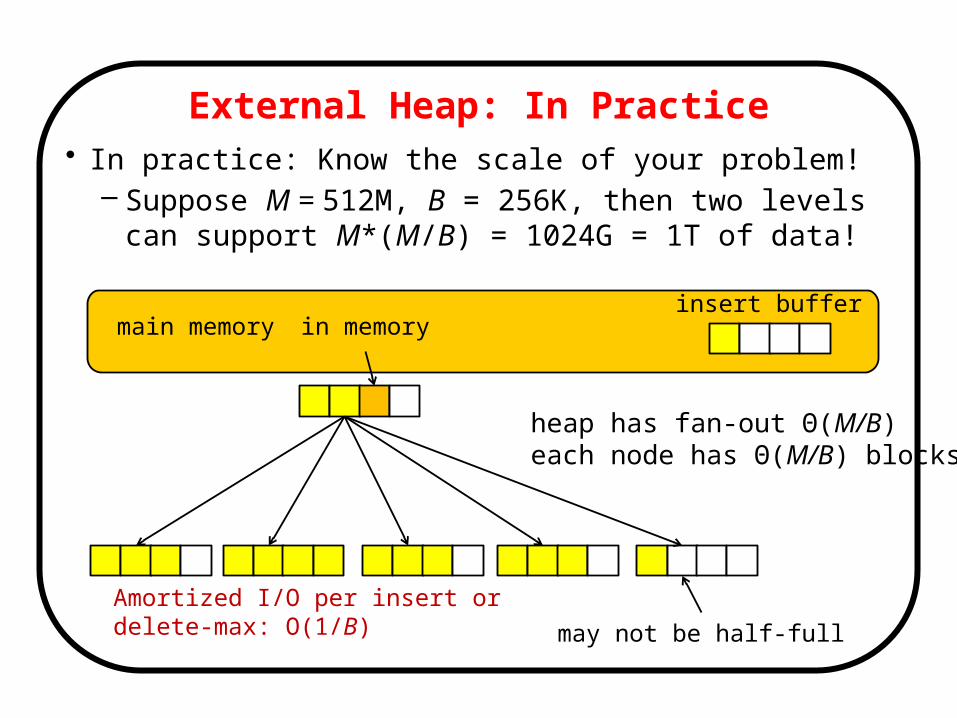
External Heap: In Practice• In practice: Know the scale of your problem!
– Suppose M = 512M, B = 256K, then two levels can support M*(M/B) = 1024G = 1T of data!
main memory
may not be half-full
insert buffer
heap has fan-out Θ(M/B) each node has Θ(M/B) blocks
in memory
Amortized I/O per insert or delete-max: O(1/B)
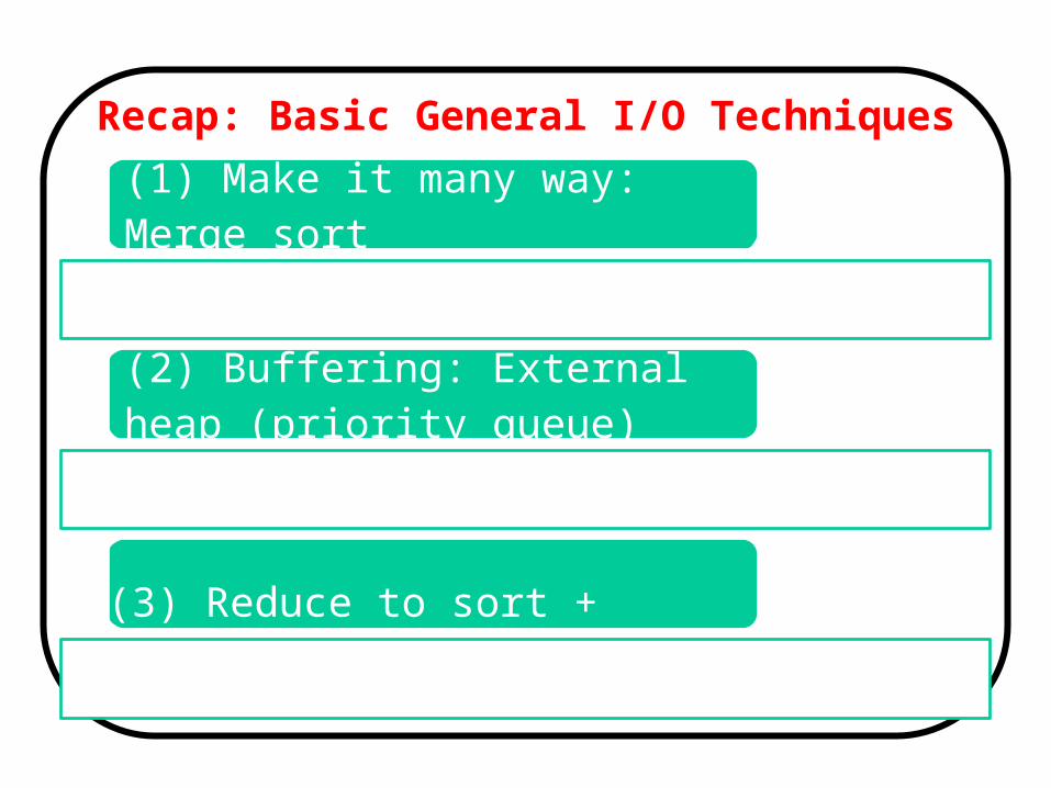
Recap: Basic General I/O Techniques
(1) Make it many way: Merge sort
(2) Buffering: External heap (priority queue)
(3) Reduce to sort + pqueue
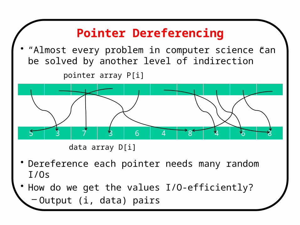
Pointer Dereferencing• “Almost every problem in computer science can be solved by
another level of indirection”
• Dereference each pointer needs many random I/Os• How do we get the values I/O-efficiently?
– Output (i, data) pairs
5 3 7 3 6 4 8 4 6 8
pointer array P[i]
data array D[i]
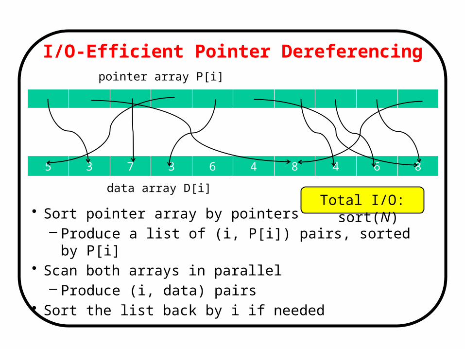
I/O-Efficient Pointer Dereferencing
• Sort pointer array by pointers– Produce a list of (i, P[i]) pairs, sorted by P[i]
• Scan both arrays in parallel– Produce (i, data) pairs
• Sort the list back by i if needed
5 3 7 3 6 4 8 4 6 8
pointer array P[i]
data array D[i]Total I/O: sort(N)
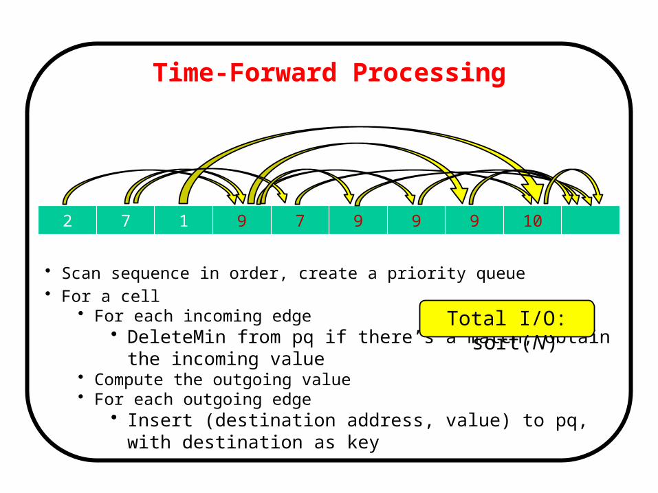
Time-Forward Processing
2 7 1 9 7 9 9 9 10
• Scan sequence in order, create a priority queue• For a cell
• For each incoming edge• DeleteMin from pq if there’s a match, obtain the incoming value
• Compute the outgoing value• For each outgoing edge
• Insert (destination address, value) to pq, with destination as key
Total I/O: sort(N)
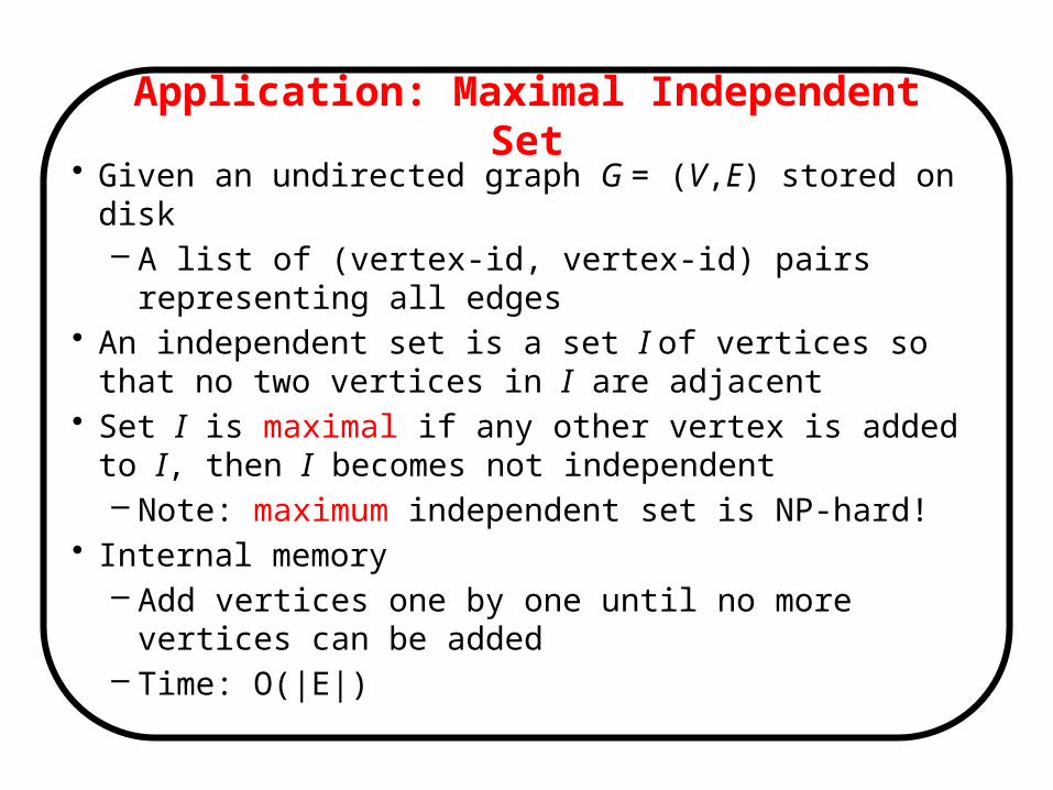
Application: Maximal Independent Set• Given an undirected graph G = (V,E) stored on disk
– A list of (vertex-id, vertex-id) pairs representing all edges• An independent set is a set I of vertices so that no two vertices in I
are adjacent• Set I is maximal if any other vertex is added to I, then I becomes not
independent– Note: maximum independent set is NP-hard!
• Internal memory– Add vertices one by one until no more vertices can be added– Time: O(|E|)
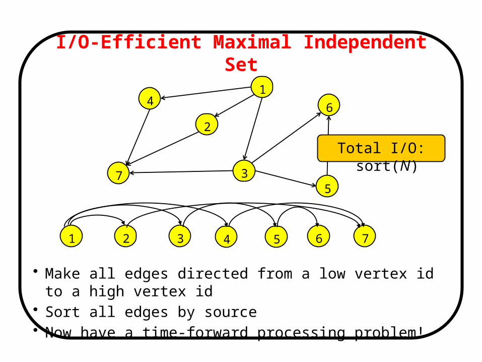
I/O-Efficient Maximal Independent Set
• Make all edges directed from a low vertex id to a high vertex id• Sort all edges by source• Now have a time-forward processing problem!
4
2
37
6
5
1
Total I/O: sort(N)
1 2 3 4 5 6 7
Big Data Algorithms
59
1980 19881999 2006
External memoryAlgorithms
Data streamAlgorithms
DistributedAlgorithms
ParallelAlgorithms

Problem One: Missing Card• I take one from a deck of 52 cards, and pass the rest to you. Suppose
you only have a (very basic) calculator and bad memory, how can you find out which card is missing with just one pass over the 51 cards?
• What if there are two missing cards?
60
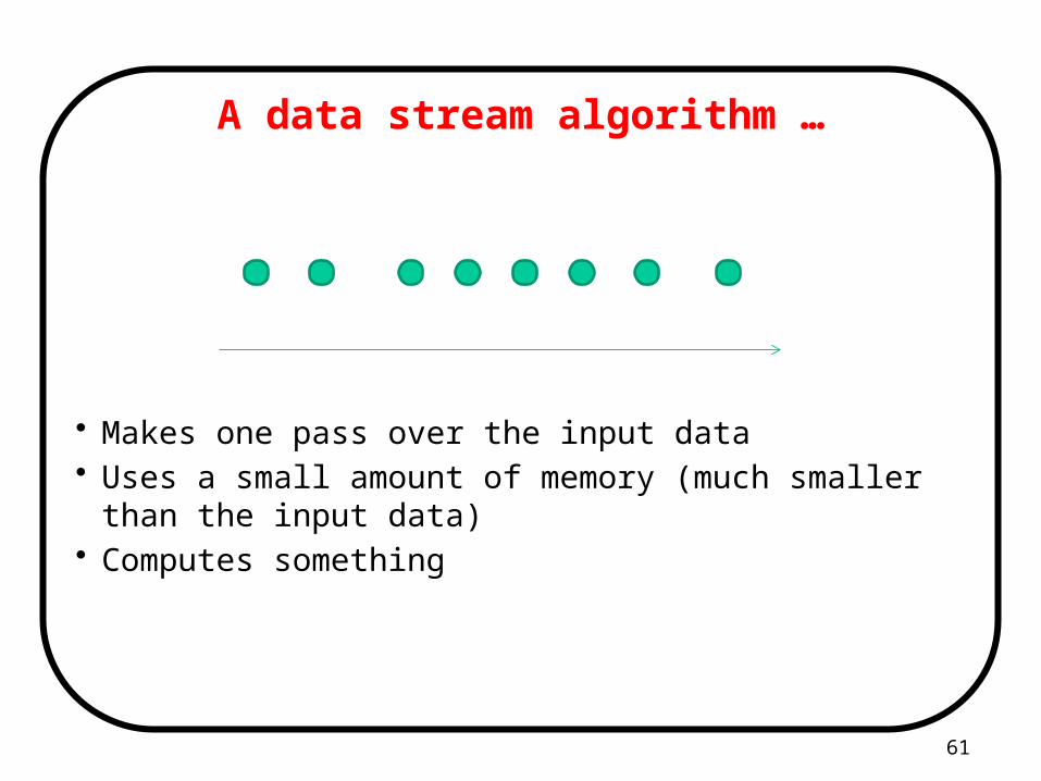
A data stream algorithm …
• Makes one pass over the input data• Uses a small amount of memory (much smaller than the input
data)• Computes something
61
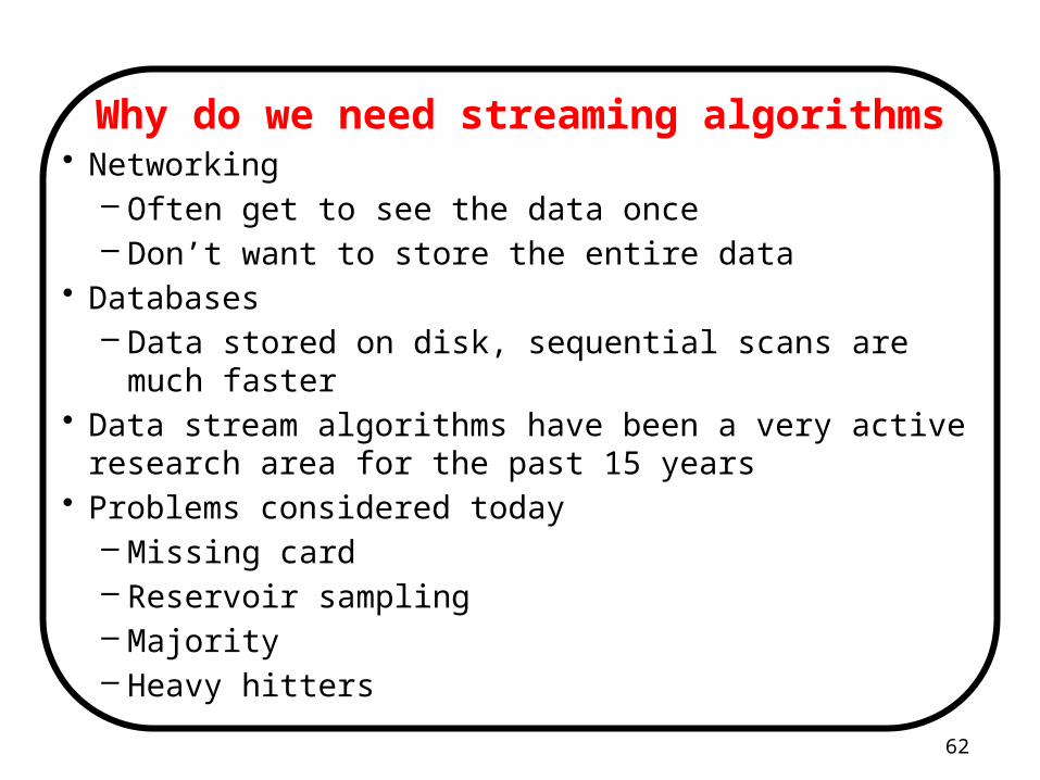
Why do we need streaming algorithms• Networking
– Often get to see the data once– Don’t want to store the entire data
• Databases– Data stored on disk, sequential scans are much faster
• Data stream algorithms have been a very active research area for the past 15 years
• Problems considered today– Missing card– Reservoir sampling– Majority– Heavy hitters
62
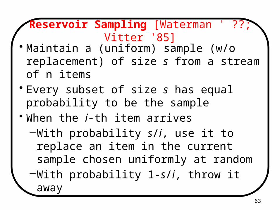
Reservoir Sampling [Waterman ' ??; Vitter '85]
• Maintain a (uniform) sample (w/o replacement) of size s from a stream of n items
• Every subset of size s has equal probability to be the sample
• When the i-th item arrives–With probability s/i, use it to replace an item in the
current sample chosen uniformly at random–With probability 1-s/i, throw it away
63
Reservoir Sampling: Correctness Proof
64

Problem two: Majority• Given a sequence of items, find the majority if there is one
• A A B C D B A A B B A A A A A A C C C D A B A A A• Answer: A
• Trivial if we have O(n) memory• Can you do it with O(1) memory and two passes?
– First pass: find the possible candidate– Second pass: compute its frequency and verify that it is > n/2
• How about one pass?– Unfortunately, no
65
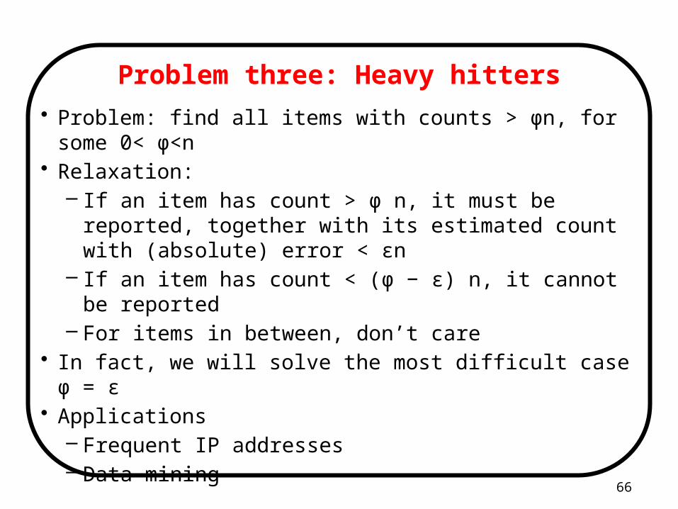
Problem three: Heavy hitters
• Problem: find all items with counts > φn, for some 0< φ<n• Relaxation:
– If an item has count > φ n, it must be reported, together with its estimated count with (absolute) error < εn
– If an item has count < (φ − ε) n, it cannot be reported– For items in between, don’t care
• In fact, we will solve the most difficult case φ = ε• Applications
– Frequent IP addresses– Data mining
66
Mergeable Summaries67
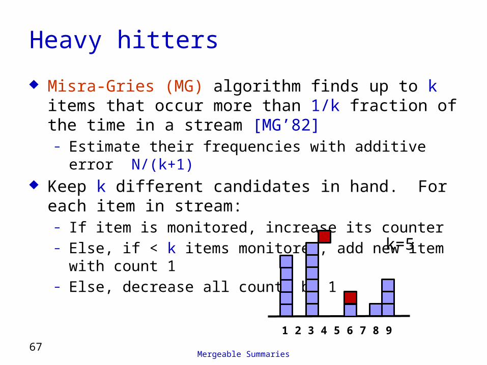
Heavy hitters
¨ Misra-Gries (MG) algorithm finds up to k items that occur more than 1/k fraction of the time in a stream [MG’82]– Estimate their frequencies with additive error N/(k+1)
¨ Keep k different candidates in hand. For each item in stream:– If item is monitored, increase its counter– Else, if < k items monitored, add new item with count 1– Else, decrease all counts by 1
1 2 3 4 5 6 7 8 9
k=5
Mergeable Summaries68
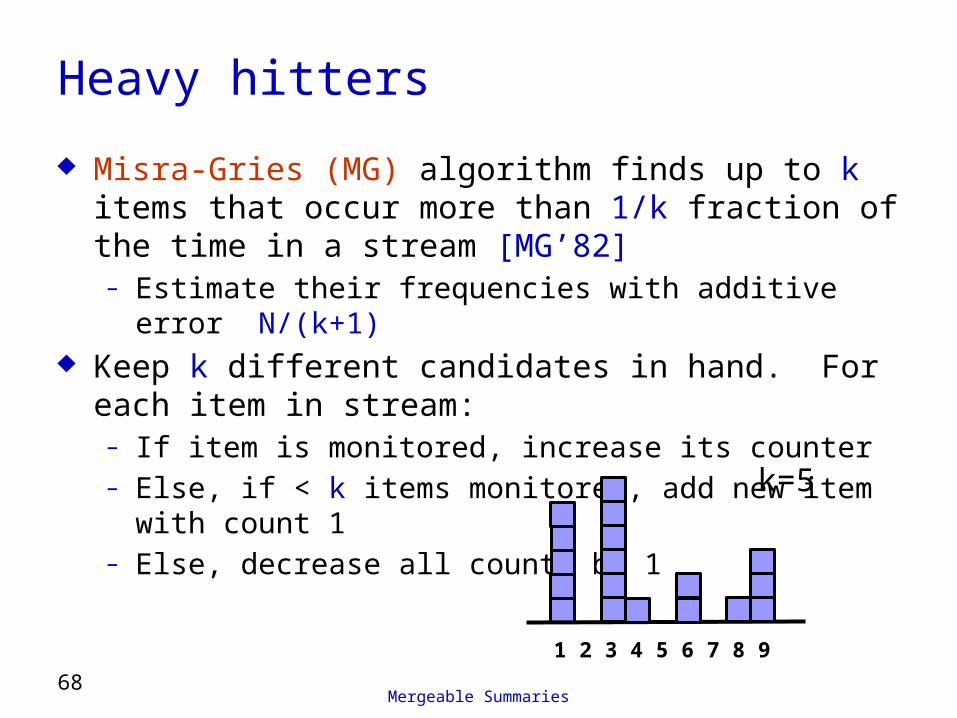
Heavy hitters
¨ Misra-Gries (MG) algorithm finds up to k items that occur more than 1/k fraction of the time in a stream [MG’82]– Estimate their frequencies with additive error N/(k+1)
¨ Keep k different candidates in hand. For each item in stream:– If item is monitored, increase its counter– Else, if < k items monitored, add new item with count 1– Else, decrease all counts by 1
1 2 3 4 5 6 7 8 9
k=5
Mergeable Summaries69
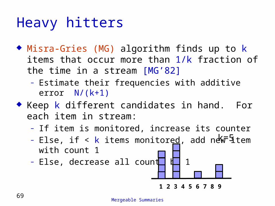
Heavy hitters
¨ Misra-Gries (MG) algorithm finds up to k items that occur more than 1/k fraction of the time in a stream [MG’82]– Estimate their frequencies with additive error N/(k+1)
¨ Keep k different candidates in hand. For each item in stream:– If item is monitored, increase its counter– Else, if < k items monitored, add new item with count 1– Else, decrease all counts by 1
1 2 3 4 5 6 7 8 9
k=5
Mergeable Summaries70
Streaming MG analysis
¨ N = total input size¨ Error in any estimated count at most N/(k+1)
– Estimated count a lower bound on true count– Each decrement spread over (k+1) items: 1 new one and k in MG– Equivalent to deleting (k+1) distinct items from stream– At most N/(k+1) decrement operations– Hence, can have “deleted” N/(k+1) copies of any item– So estimated counts have at most this much error
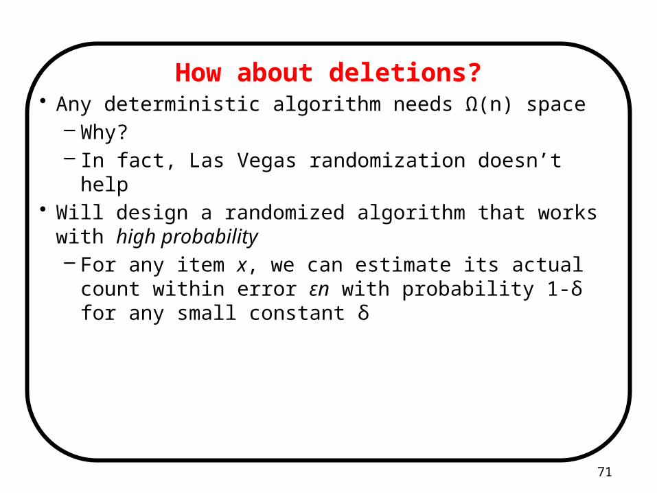
How about deletions?• Any deterministic algorithm needs Ω(n) space
– Why?– In fact, Las Vegas randomization doesn’t help
• Will design a randomized algorithm that works with high probability– For any item x, we can estimate its actual count within error εn
with probability 1-δ for any small constant δ
71
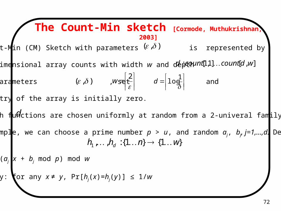
The Count-Min sketch [Cormode, Muthukrishnan, 2003]
72
A Count-Min (CM) Sketch with parameters is represented by
a two-dimensional array counts with width w and depth
Given parameters , set and .
Each entry of the array is initially zero.
hash functions are chosen uniformly at random from a 2-univeral family
For example, we can choose a prime number p > u, and random aj, bj, j=1,…,d. Define:
hj(x) = (aj x + bj mod p) mod w
Property: for any x ≠ y, Pr[hj(x)=hj(y)] ≤ 1/w
),(
],[]1,1[: wdcountcountd
),(
2
w
1
logd
d
}1{}1{:,,1 wnhh d
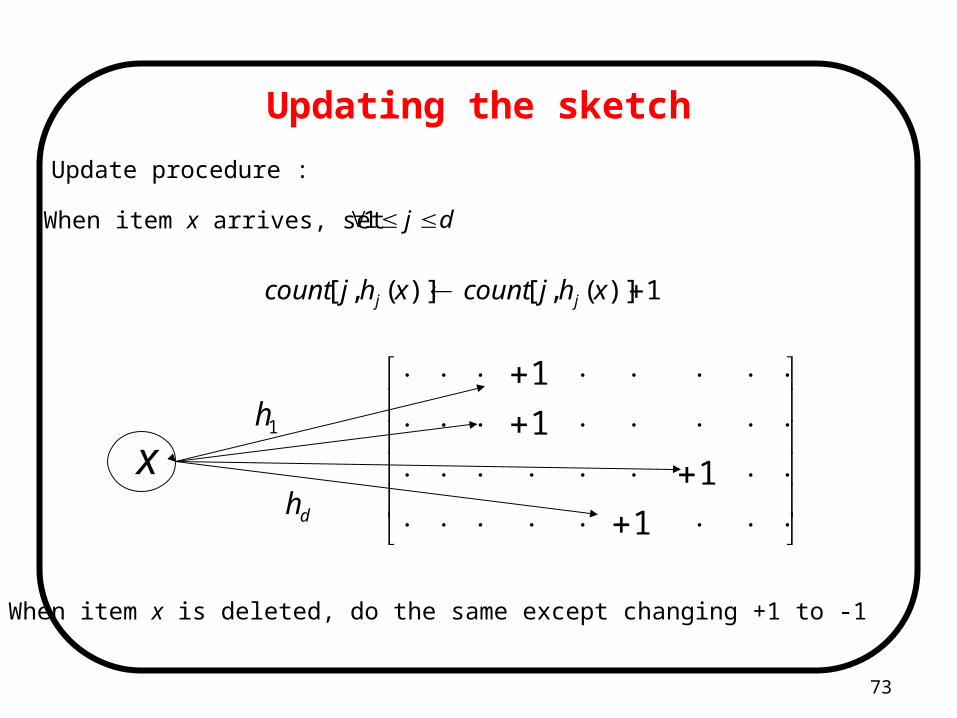
Updating the sketch
73
Update procedure :
When item x arrives, set dj 1
1)](,[)](,[ xhjcountxhjcount jj
1
1
1
1
x1h
dh
When item x is deleted, do the same except changing +1 to -1
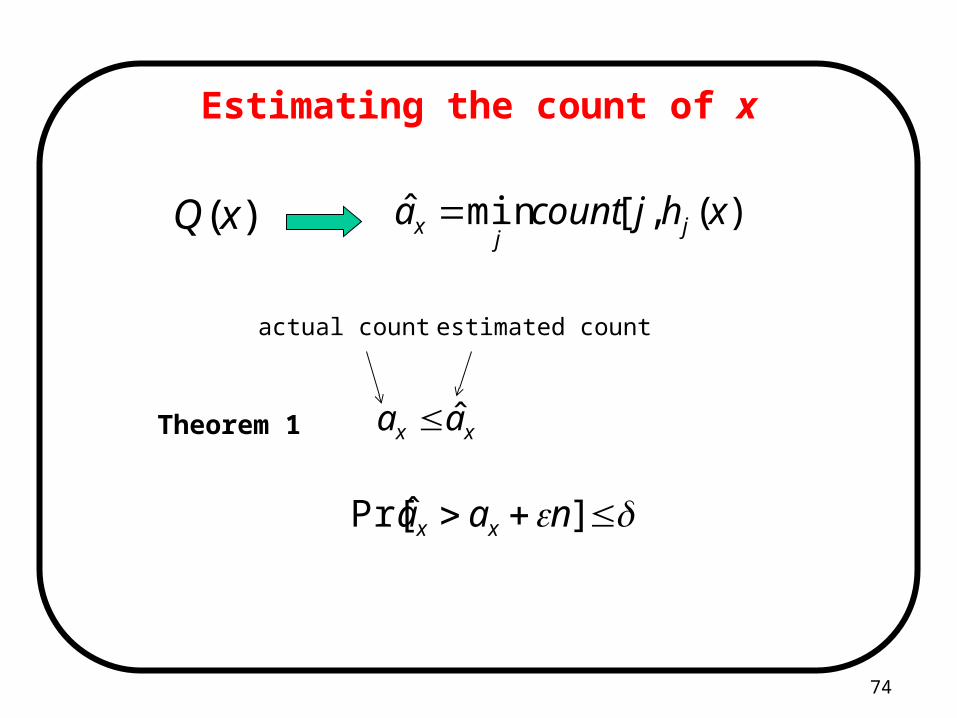
Estimating the count of x
74
)(xQ )](,[minˆ xhjcounta jj
x
Theorem 1 xx aa ˆ
]ˆPr[ naa xx
actual count estimated count
Proof
75
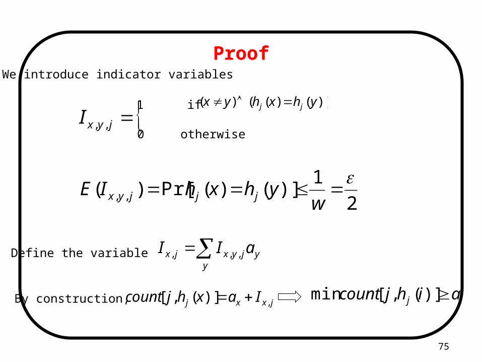
We introduce indicator variables
jyxI ,, ))()(()( yhxhyx jj 1 if
0 otherwise
2
1)]()(Pr[)( ,,
wyhxhIE jjjyx
Define the variable y
yjyxjx aII ,,,
By construction, jxxj Iaxhjcount ,)](,[ ij aihjcount )](,[min
76
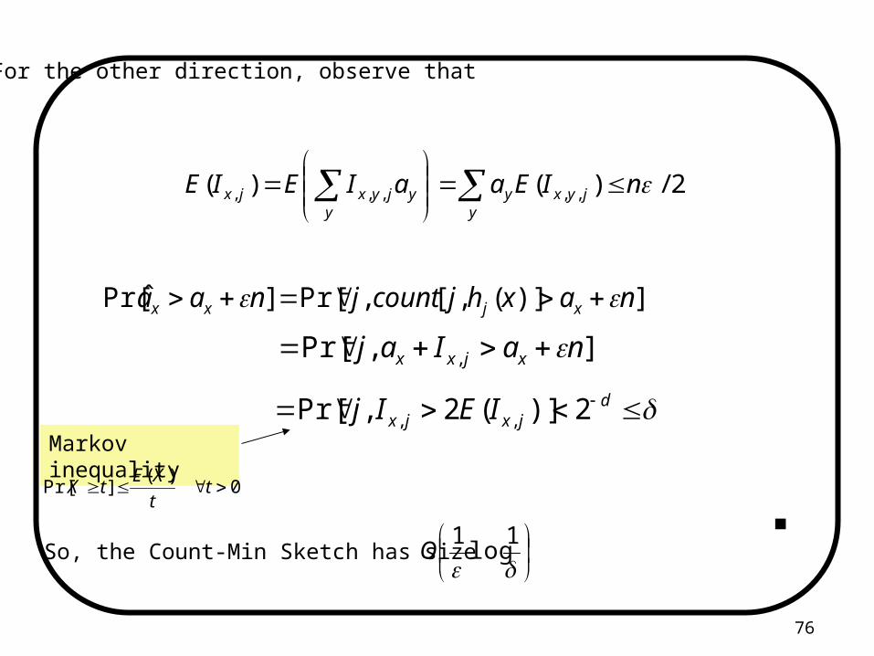
For the other direction, observe that
])](,[,Pr[]ˆPr[ naxhjcountjnaa xjxx
],Pr[ , naIaj xjxx
djxjx IEIj 2)](2,Pr[ ,,
Markov inequality
0)(
]Pr[ tt
XEtX
■
2/)()( ,,,,,
yjyxy
yyjyxjx nIEaaIEIE
So, the Count-Min Sketch has size
1
log1
O
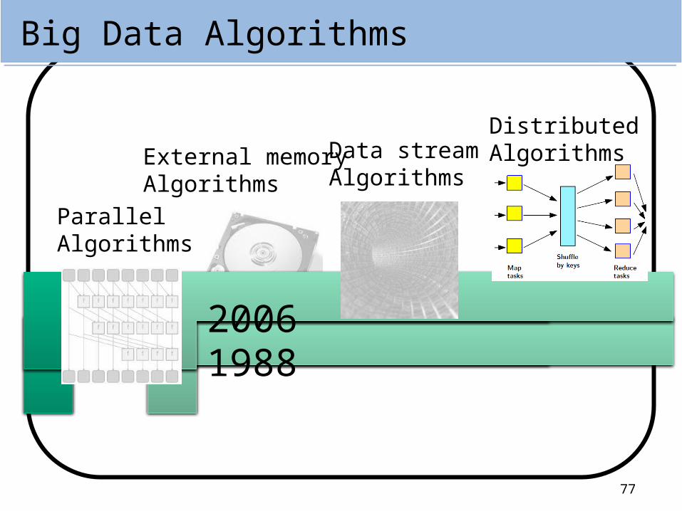
Big Data Algorithms
77
1980 19881999 2006
External memoryAlgorithms
Data streamAlgorithms
DistributedAlgorithms
ParallelAlgorithms
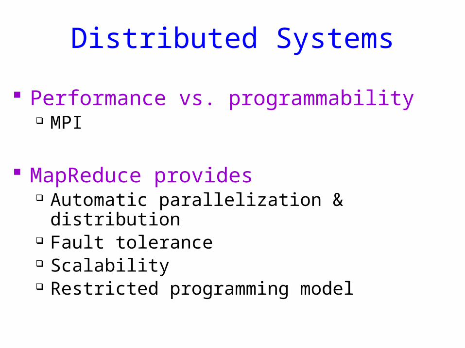
Distributed Systems
Performance vs. programmability MPI
MapReduce provides Automatic parallelization & distribution Fault tolerance Scalability Restricted programming model
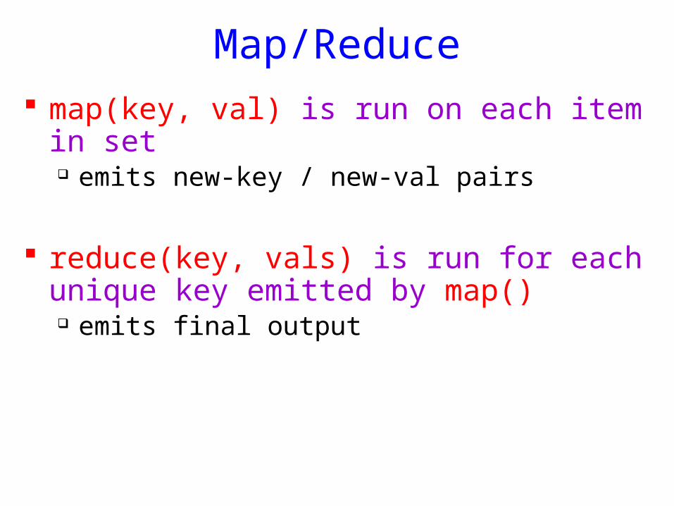
Map/Reduce map(key, val) is run on each item in set
emits new-key / new-val pairs
reduce(key, vals) is run for each unique key emitted by map() emits final output
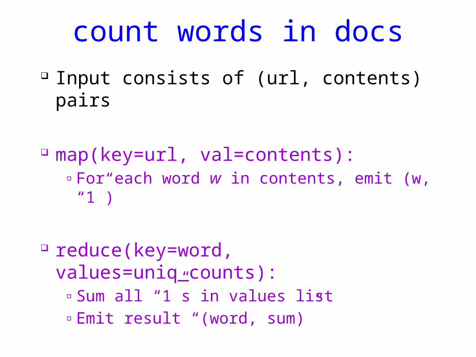
count words in docs Input consists of (url, contents) pairs
map(key=url, val=contents):▫ For each word w in contents, emit (w, “1”)
reduce(key=word, values=uniq_counts):▫ Sum all “1”s in values list▫ Emit result “(word, sum)”
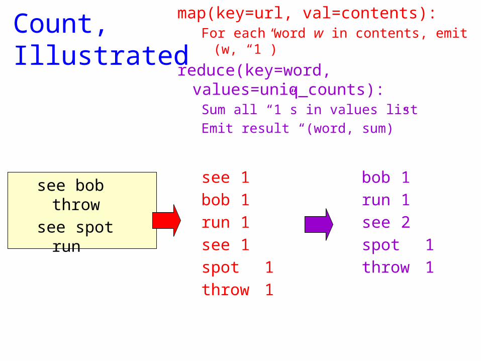
Count, Illustrated
map(key=url, val=contents):For each word w in contents, emit (w,
“1”)
reduce(key=word, values=uniq_counts):
Sum all “1”s in values listEmit result “(word, sum)”
see bob throwsee spot run
see 1bob 1 run 1see 1spot 1throw 1
bob 1 run 1see 2spot 1throw 1
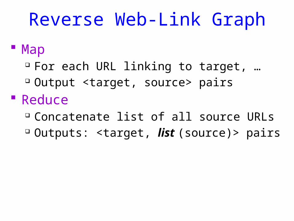
Reverse Web-Link Graph Map
For each URL linking to target, … Output <target, source> pairs
Reduce Concatenate list of all source URLs Outputs: <target, list (source)> pairs
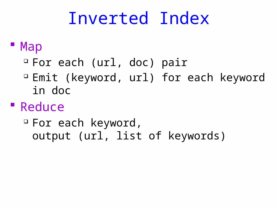
Inverted Index Map
For each (url, doc) pair Emit (keyword, url) for each keyword in doc
Reduce For each keyword,
output (url, list of keywords)
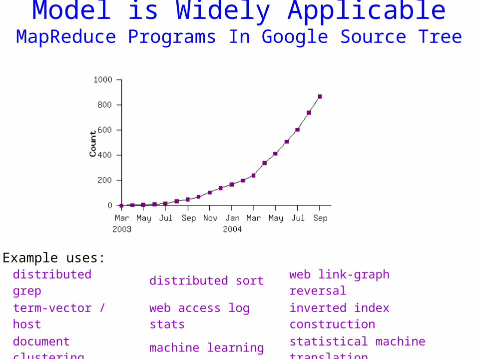
Example uses: distributed grep distributed sort web link-graph reversal
term-vector / host web access log stats
inverted index construction
document clustering machine learning statistical machine
translation
... ... ...
Model is Widely ApplicableMapReduce Programs In Google Source Tree
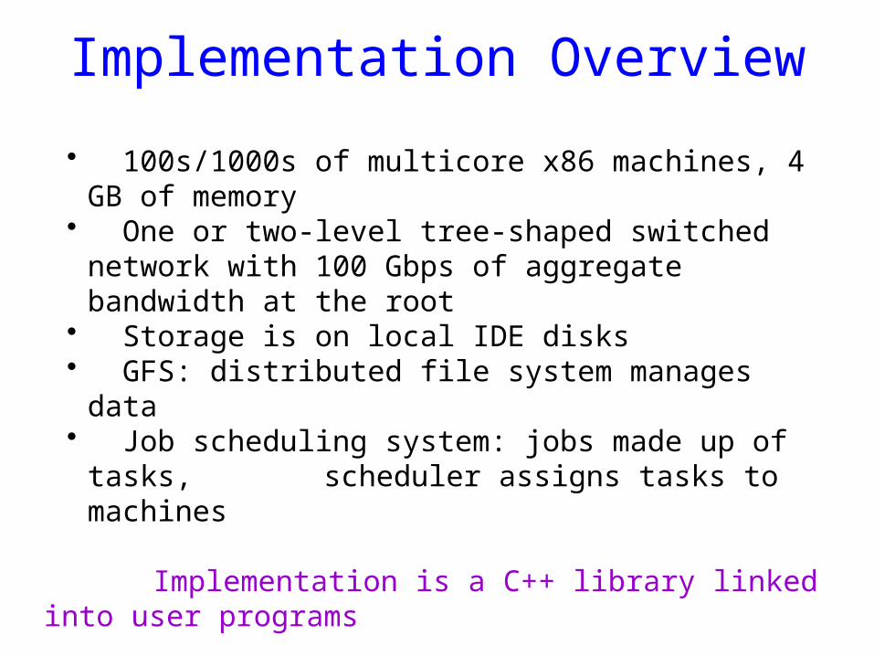
Typical cluster:
• 100s/1000s of multicore x86 machines, 4 GB of memory • One or two-level tree-shaped switched network with 100
Gbps of aggregate bandwidth at the root • Storage is on local IDE disks • GFS: distributed file system manages data • Job scheduling system: jobs made up of tasks,
scheduler assigns tasks to machines
Implementation is a C++ library linked into user programs
Implementation Overview
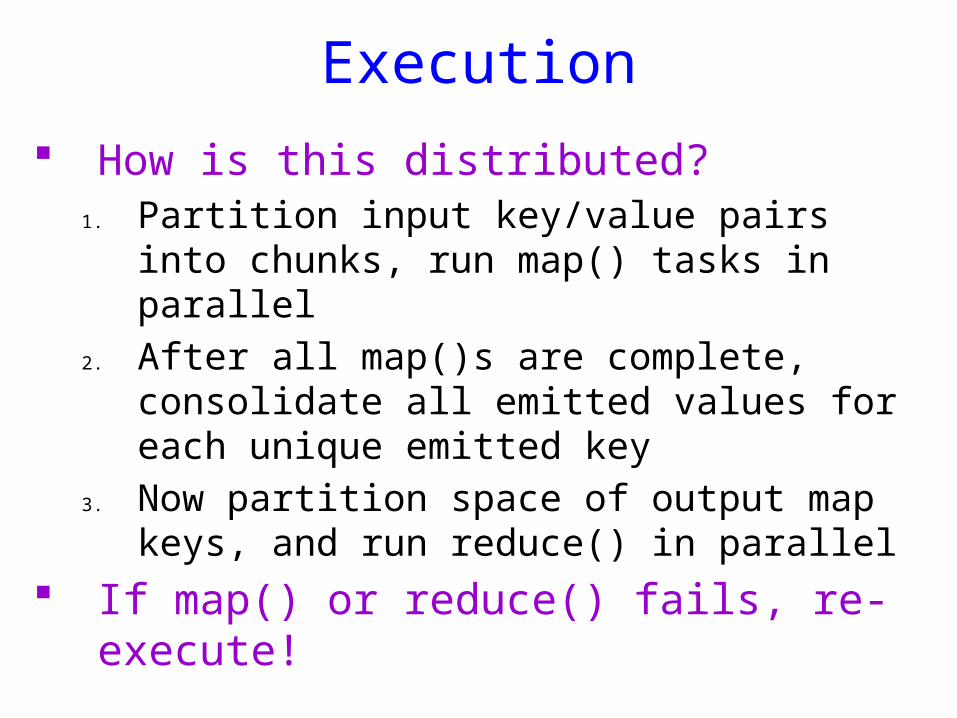
Execution How is this distributed?
1. Partition input key/value pairs into chunks, run map() tasks in parallel
2. After all map()s are complete, consolidate all emitted values for each unique emitted key
3. Now partition space of output map keys, and run reduce() in parallel
If map() or reduce() fails, re-execute!
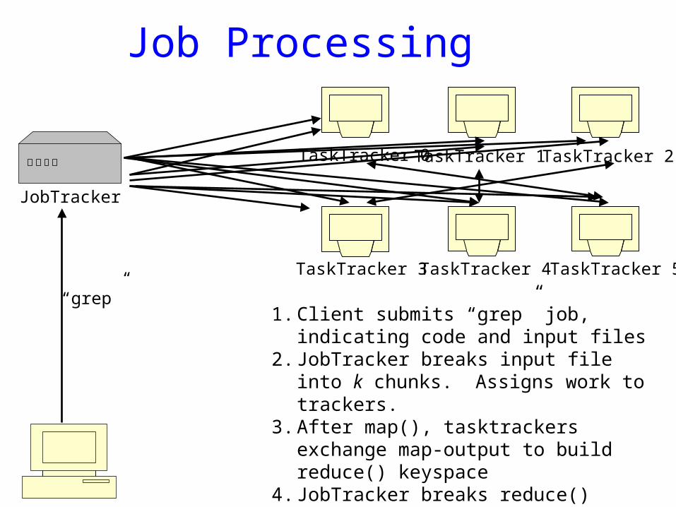
Job Processing
JobTracker
TaskTracker 0TaskTracker 1 TaskTracker 2
TaskTracker 3 TaskTracker 4 TaskTracker 5
1. Client submits “grep” job, indicating code and input files
2. JobTracker breaks input file into k chunks. Assigns work to trackers.
3. After map(), tasktrackers exchange map-output to build reduce() keyspace
4. JobTracker breaks reduce() keyspace into m chunks. Assigns work.
5. reduce() output may go to NDFS
“grep”
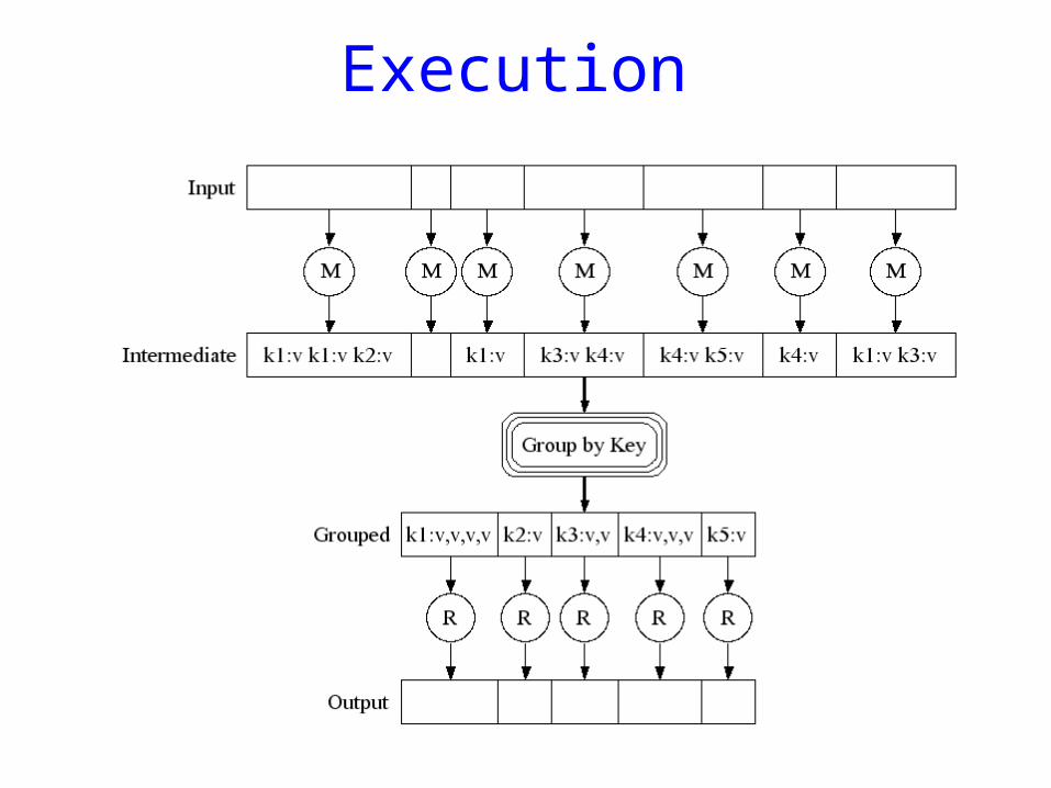
Execution
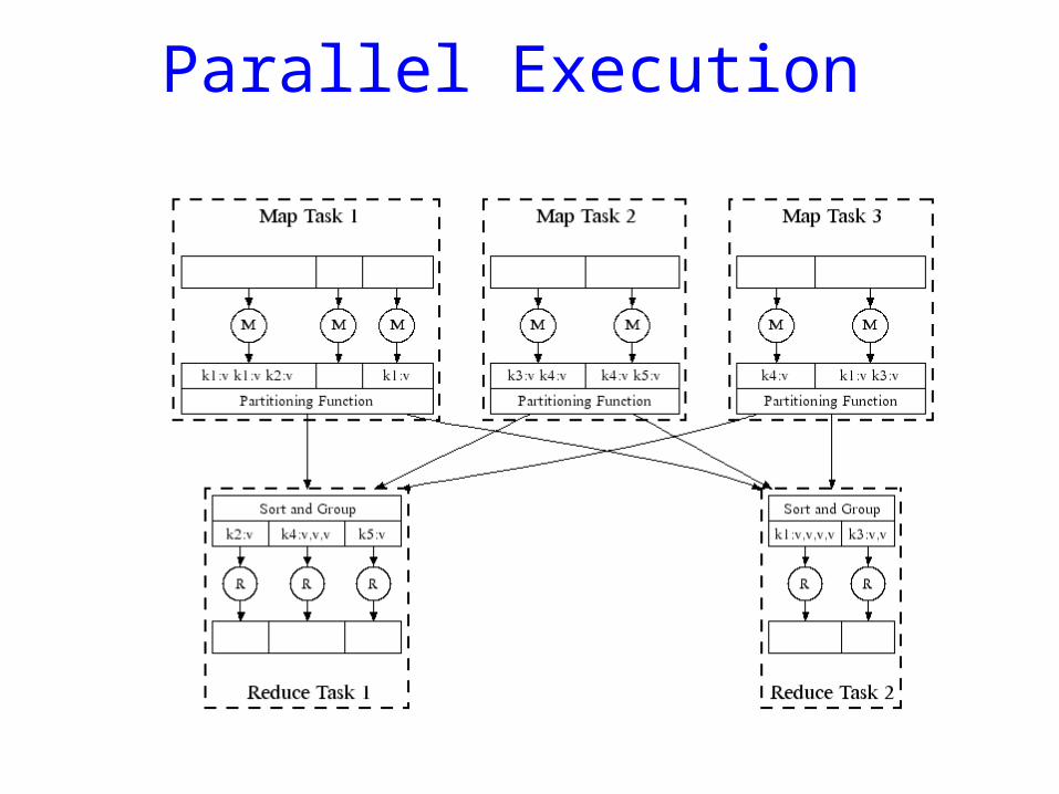
Parallel Execution
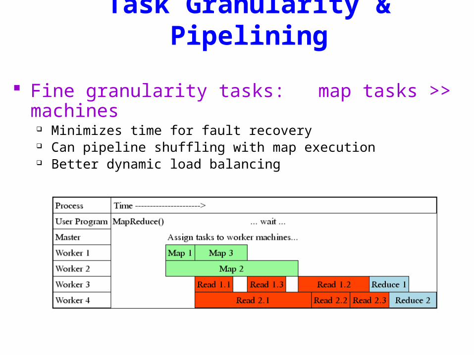
Task Granularity & Pipelining
Fine granularity tasks: map tasks >> machines Minimizes time for fault recovery Can pipeline shuffling with map execution Better dynamic load balancing
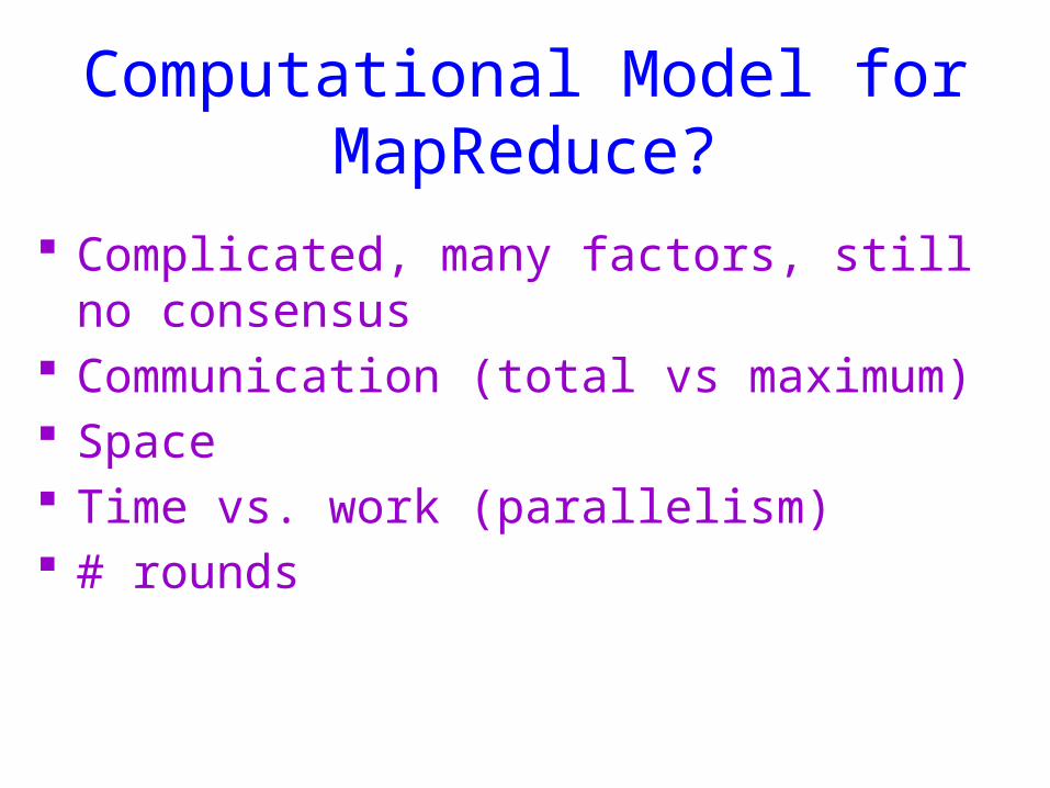
Computational Model for MapReduce?
Complicated, many factors, still no consensus
Communication (total vs maximum) Space Time vs. work (parallelism) # rounds
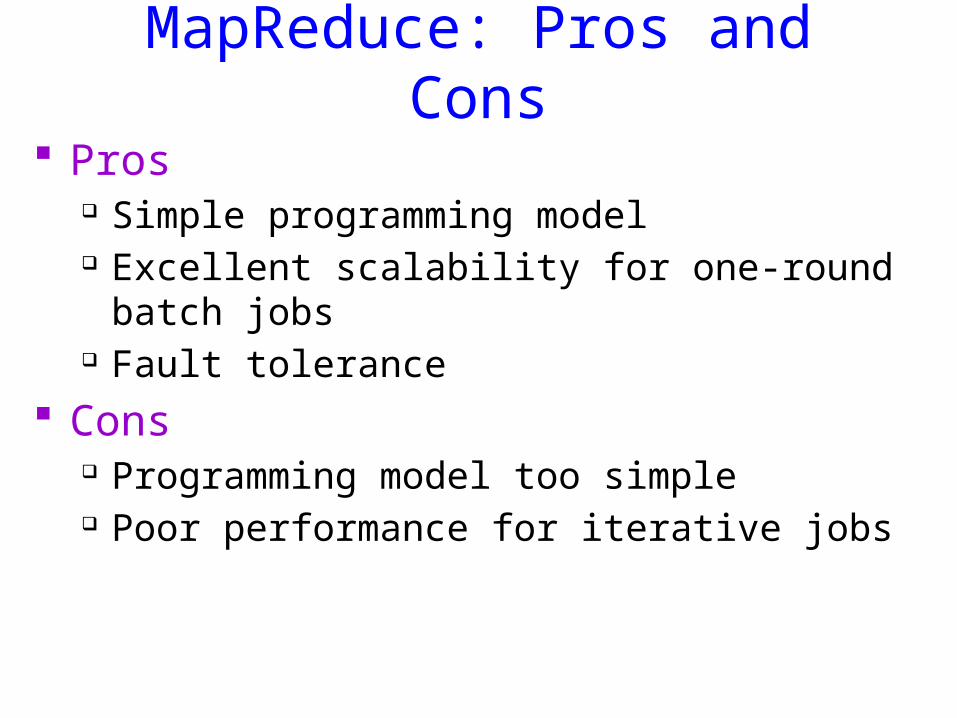
MapReduce: Pros and Cons Pros
Simple programming model Excellent scalability for one-round batch
jobs Fault tolerance
Cons Programming model too simple Poor performance for iterative jobs
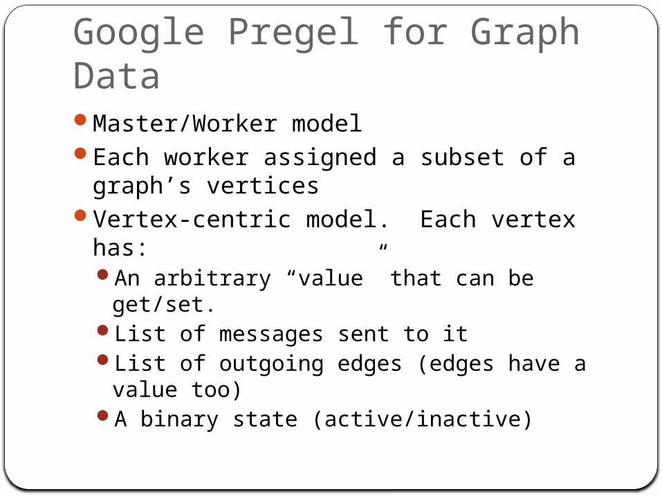
Google Pregel for Graph DataMaster/Worker modelEach worker assigned a subset of a graph’s
verticesVertex-centric model. Each vertex has:
An arbitrary “value” that can be get/set.List of messages sent to itList of outgoing edges (edges have a value
too)A binary state (active/inactive)

The Pregel modelBulk Synchronous Parallel model (Valiant, 95)
Synchronous iterations of asynchronous computationMaster initiates each iteration (called a “superstep”)At every superstep
Workers asynchronously execute a user function on all of its vertices
Vertices can receive messages sent to it in the last superstepVertices can send messages to other vertices to be received in
the next superstepVertices can modify their value, modify values of edges, change
the topology of the graph (add/remove vertices or edges)Vertices can “vote to halt”
Execution stops when all vertices have voted to halt and no vertices have messages.
Vote to halt trumped by non-empty message queue
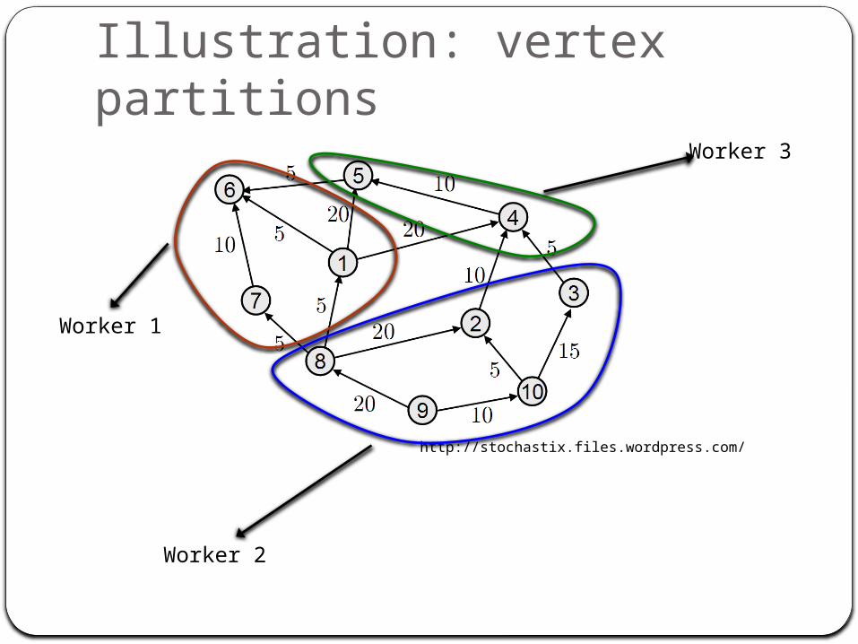
Illustration: vertex partitions
http://stochastix.files.wordpress.com/
Worker 1
Worker 2
Worker 3
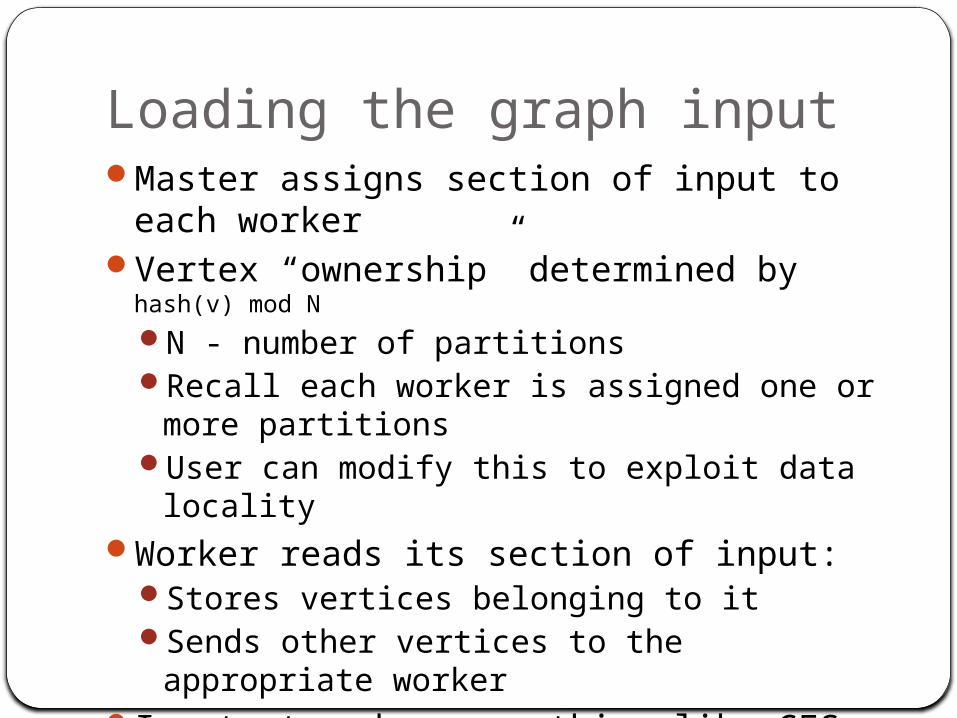
Loading the graph inputMaster assigns section of input to each
workerVertex “ownership” determined by hash(v) mod N
N - number of partitionsRecall each worker is assigned one or more
partitionsUser can modify this to exploit data locality
Worker reads its section of input:Stores vertices belonging to itSends other vertices to the appropriate
workerInput stored on something like GFS
Section assignments determined by data locality
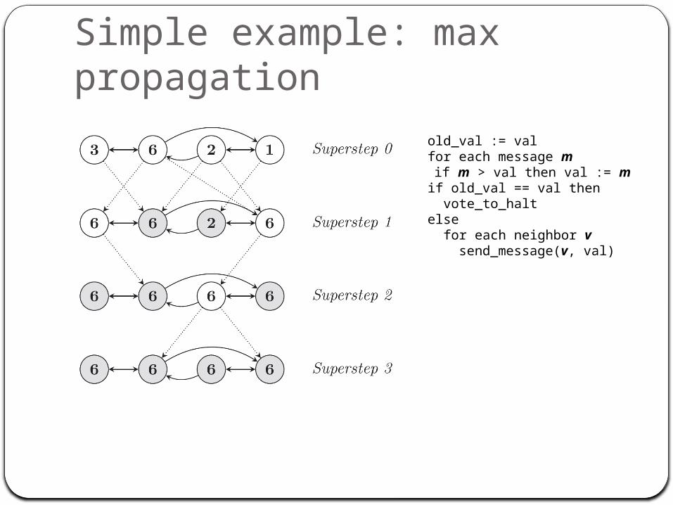
Simple example: max propagation
old_val := valfor each message m if m > val then val := mif old_val == val then vote_to_haltelse for each neighbor v send_message(v, val)
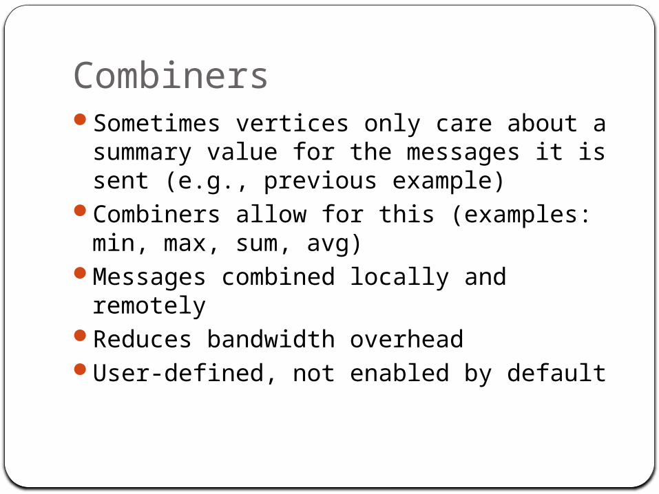
CombinersSometimes vertices only care about a
summary value for the messages it is sent (e.g., previous example)
Combiners allow for this (examples: min, max, sum, avg)
Messages combined locally and remotelyReduces bandwidth overhead User-defined, not enabled by default
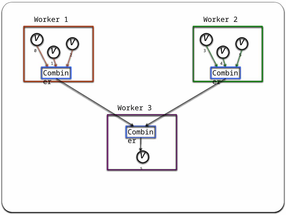
Worker 1
v0 v
1
v2
Combiner
Worker 2
v3 v
4
v5
Combiner
Worker 3
vs
Combiner
AggregatorsCompute aggregate statistics from vertex-
reported valuesDuring a superstep, each worker
aggregates values from its vertices to form a partially aggregated value
At the end of a superstep, partially aggregated values from each worker are aggregated in a tree structure Allows for the parallelization of this process
Global aggregate is sent to the master
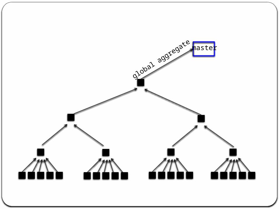
master
global aggregate
Fault Tolerance (1/2)At start of superstep, master tells workers
to save their state:Vertex values, edge values, incoming
messagesSaved to persistent storage
Master saves aggregator values (if any)This isn’t necessarily done at every
superstepThat could be very costlyAuthors determine checkpoint frequency
using mean time to failure model
Fault Tolerance (2/2)When master detects one or more worker
failures:All workers revert to last checkpointContinue from thereThat’s a lot of repeated work! At least it’s better than redoing the whole
thing.
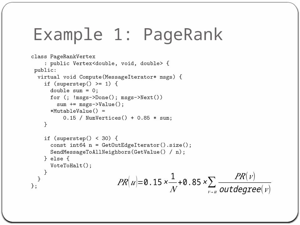
Example 1: PageRank
𝑃𝑅 (𝑢)=0.15×1𝑁
+0.85 × ∑𝑣→𝑢
𝑃𝑅(𝑣)outdegree(𝑣)
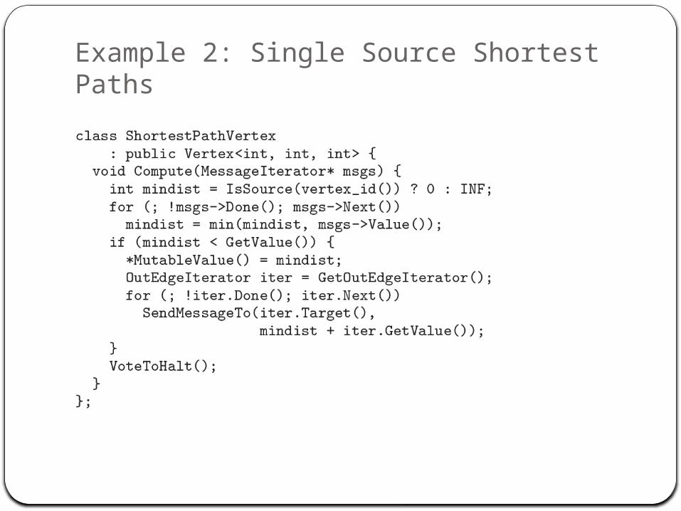
Example 2: Single Source Shortest Paths
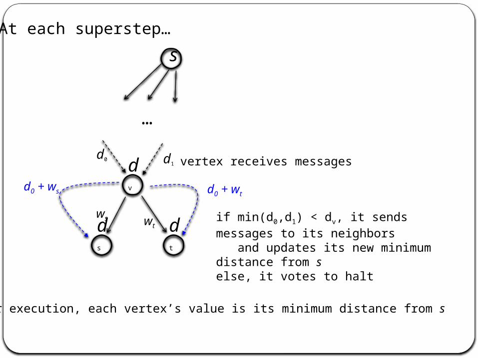
s
dv
At each superstep…
…
vertex receives messagesd0 d1
ds
dt
ws wtif min(d0,d1) < dv, it sends messages to its neighbors and updates its new minimum distance from selse, it votes to halt
d0 + ws d0 + wt
After execution, each vertex’s value is its minimum distance from s
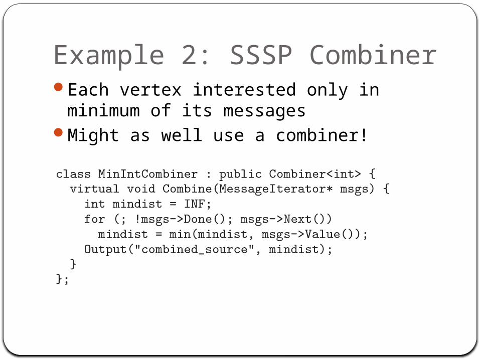
Example 2: SSSP CombinerEach vertex interested only in minimum of
its messagesMight as well use a combiner!
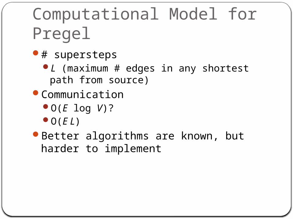
Computational Model for Pregel# supersteps
L (maximum # edges in any shortest path from source)
CommunicationO(E log V)?O(E L)
Better algorithms are known, but harder to implement

Conclusions Algorithm design facing new
constraints/challenges in the big data era
Resources other than time may be the main consideration
Data movement cost often the primary concern
Algorithmic ideas often independent of technological improvements

Thank you!