BIG O Notation Time Complexity and Space Complexity · BIG O Notation – Time Complexity and Space Complexity ... Conditional checks: ... Time Complexity and Space Complexity ) )

BIG O Notation – Time Complexity and Space Complexity

In computer science, big O notation is used to classify algorithms by how they respond (e.g., in their

processing time or working space requirements) to changes in input size.

For a general example that is understandable:

Pick a number between 1 and 1000. I guess 500. You say "higher". I guess 750. You say "lower." I choose

625... Clearly my search is not going to take 1000 guesses (order n). I chop my search domain in half

each time and take 10 guesses or less

"If I have n items and each time through the loop I can throw out half of them, how many times do I

have to go through the loop until there's only one remaining?" This is the analysis for binary sort. If I've

gone through the loop k times, then I have 1/2^k items remaining. So I want to find k such that n/2^k =

1. This is the same as n=2^k or k = log2n.

Beginners Guide:

Big O notation is used in Computer Science to describe the performance or complexity of an algorithm.

Big O specifically describes the worst-case scenario, and can be used to describe the execution time

required or the space used (e.g. in memory or on disk) by an algorithm.

O(1)

O(1) describes an algorithm that will always execute in the same time (or space) regardless of the size of

the input data set.

bool IsFirstElementNull(String[] strings)

{

if(strings[0] == null)

{

return true;

}

return false;

}

O(N)

O(N) describes an algorithm whose performance will grow linearly and in direct proportion to the size of

the input data set. The example below also demonstrates how Big O favors the worst-case performance

scenario; a matching string could be found during any iteration of the for loop and the function would

return early, but Big O notation will always assume the upper limit where the algorithm will perform the

maximum number of iterations.

bool ContainsValue(String[] strings, String value)

{

for(int i = 0; i < strings.Length; i++)

{


if(strings[i] == value)

{

return true;

}

}

return false;

}

O(N2)

O(N2) represents an algorithm whose performance is directly proportional to the square of the size of

the input data set. This is common with algorithms that involve nested iterations over the data set.

Deeper nested iterations will result in O(N3), O(N4) etc.

bool ContainsDuplicates(String[] strings)

{

for(int i = 0; i < strings.Length; i++)

{

for(int j = 0; j < strings.Length; j++)

{

if(i == j) // Don't compare with self

{

continue;

}

if(strings[i] == strings[j])

{

return true;

}

}

}

return false;

}

O(2N)

O(2N) denotes an algorithm whose growth will double with each additional element in the input data

set. The execution time of an O(2N) function will quickly become very large.

Logarithms

Logarithms are slightly trickier to explain so I’ll use a common example:


Binary search is a technique used to search sorted data sets. It works by selecting the middle element of

the data set, essentially the median, and compares it against a target value. If the values match it will

return success. If the target value is higher than the value of the probe element it will take the upper

half of the data set and perform the same operation against it. Likewise, if the target value is lower than

the value of the probe element it will perform the operation against the lower half. It will continue to

halve the data set with each iteration until the value has been found or until it can no longer split the

data set.

This type of algorithm is described as O(log N). The iterative halving of data sets described in the binary

search example produces a growth curve that peaks at the beginning and slowly flattens out as the size

of the data sets increase e.g. an input data set containing 10 items takes one second to complete, a data

set containing 100 items takes two seconds, and a data set containing 1000 items will take three

seconds. Doubling the size of the input data set has little effect on its growth as after a single iteration of

the algorithm the data set will be halved and therefore on a par with an input data set half the size. This

makes algorithms like binary search extremely efficient when dealing with large data sets.

Computational Complexity: It is very interesting and useful as it helps a programmer to find out the the

complexity of a set of possible algorithms for a particular programming task, thus helping him to select

the algorithm with minimum complexity in terms of number of instructions involved. So here we will

explain what is Computational Complexity, Big O notation to compare algorithms and analysis of the

most popular searching and sorting methods.

What is an algorithm: An algorithm is a sequence of instructions that act on some input data to produce

some output in a finite number of steps.

Why analyze algorithm: Determining which algorithm is efficient than the other involves analysis of

algorithms.

Factors considered in analysis: Two factors considered while analyzing algorithms are time and space.

Time: Actual run time on a particular computer is not a good basis for comparison since it

depends heavily on the speed of the computer, the total amount of RAM, the Operating System

running on the system and the quality of the computer used. So the complexity of an algorithm

is the number of elementary instructions performed with respect to the size of the input data.

Space: This is a less important factor than time because if more space is required, it can always

be found in the form of auxiliary storage.

What is Computational Complexity: It refers to the measure of the performance of an algorithm. It

allows the comparison of algorithm for efficiency and predicts their behavior as data size increases.

Dominant Term: While describing the growth rate of an algorithm, we simply consider the term which

affects the most on the algorithm’s performance. This term is known as the dominant term.


Example:

//to count no. of characters in a file

count=0

While(there are more characters in a file) do

increment count by 1

get the next character

End While

Print count

In the above example, no of various instructions for a file size of 500 characters,

Initialization: 1 instruction

Increments: 500

Conditional checks: 500 + 1 (for eof)

Printing: 1

Initialization and Printing is same for any size of file so they are insignificant compared to increments

and checks. So increments and checks are the dominant terms in the above example.

Best, Average and Worst Case Complexity: In most algorithms, the actual complexity for a particular

input can vary. E.g. If input list is sorted, linear search may perform poorly while binary search will

perform very well. Hence, multiple input sets must be considered while analyzing an algorithm. These

include the following

1. Best Case Input: This represents the input set that allows an algorithm to perform most quickly.

With this input, the algorithm takes the shortest time to execute, as it causes the algorithms to

do the least amount of work. It provides the way an algorithm behaves under optimal

conditions. E.g. In a searching algorithm, if match is found at the first location, it is the best case

input as the no. comparisons is just one.

2. Worst Case Input: This represents the input set that allows an algorithm to perform most

slowly. It is an important analysis because it gives us an idea of the maximum time an algorithm

will ever take. It is important because it provides an upper bound on running time of an

algorithm. And it is also a promise that the algorithm will not take more than the calculated

time. Eg. In a searching algorithm, if value to be searched is at the last location or it is not in the

list, is the worst case input because it tells the maximum number of comparisons that have to be

made.


3. Average Case Input: This represents the input set that allows an algorithm to deliver an average

performance. It provides the expected running time. It needs assumption of statistical

distribution of inputs.

Rate of growth: The growth rate determines the algorithm’s performance when the input size grows.

Big O Notation: The Big O Notation is a class of mathematical formula that best describes an algorithm’s

growth rate. It is very useful:

1. For comparing the performance of two or more algorithms.

2. It frees us from bothering about constants.

Let f(n) , g(n) be two functions. Then, f(n) is O(g(n)) if there exists constants a, b such that :

F(n) <= a * g(n) whenever n>=b

E.g. If, f(n) = n2 + 100n

and, g(n) = n2 , and a=2 , and b=100

then, f(n) is O(g(n))

Because (n2 + 100n) is less than or equal to (2n2) for all n greater than or equal to 100.

It means that eventually for n>=b, f(n) becomes permanently smaller or equal to some multiple of g(n).

In other words, f(n) is a smaller function than g(n) or f(n) is asymptotically bounded by g(n) or f(n) grows

slower than g(n) or g(n) does not better than f(n) in solving the problem.

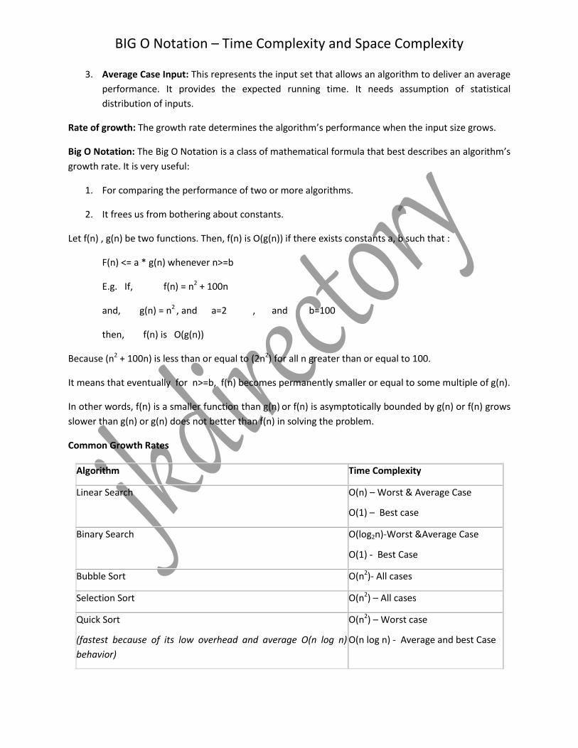
Common Growth Rates

Algorithm Time Complexity

Linear Search O(n) – Worst & Average Case

O(1) – Best case

Binary Search O(log2n)-Worst &Average Case

O(1) - Best Case

Bubble Sort O(n2)- All cases

Selection Sort O(n2) – All cases

Quick Sort

(fastest because of its low overhead and average O(n log n)

behavior)

O(n2) – Worst case

O(n log n) - Average and best Case


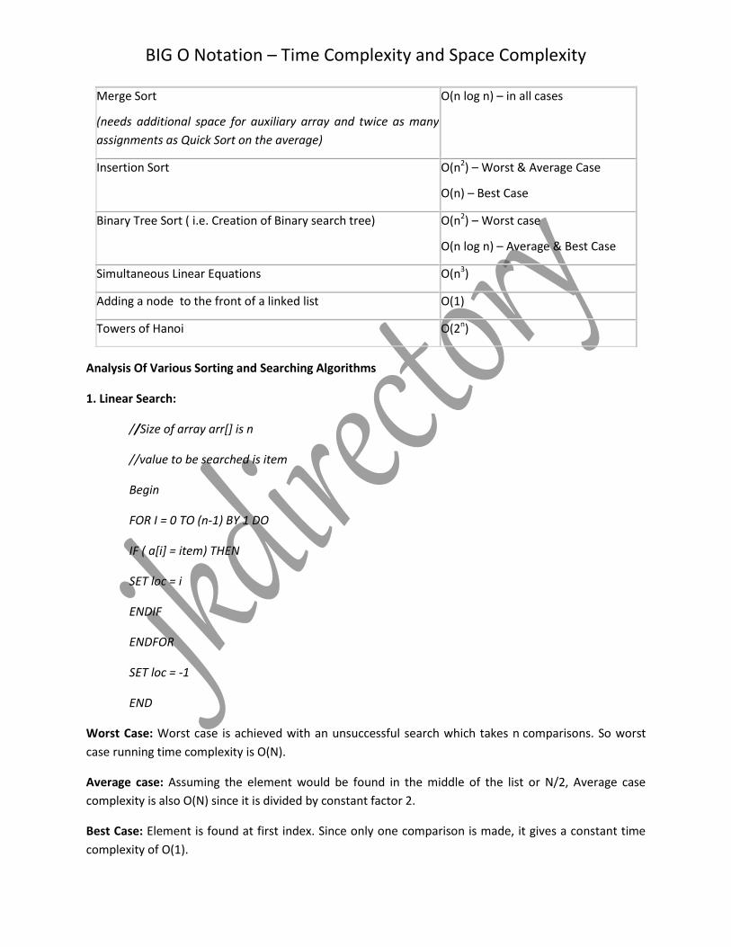
Analysis Of Various Sorting and Searching Algorithms

1. Linear Search:

//Size of array arr[] is n

//value to be searched is item

Begin

FOR I = 0 TO (n-1) BY 1 DO

IF ( a[i] = item) THEN

SET loc = i

ENDIF

ENDFOR

SET loc = -1

END

Worst Case: Worst case is achieved with an unsuccessful search which takes n comparisons. So worst

case running time complexity is O(N).

Average case: Assuming the element would be found in the middle of the list or N/2, Average case

complexity is also O(N) since it is divided by constant factor 2.

Best Case: Element is found at first index. Since only one comparison is made, it gives a constant time

complexity of O(1).

Merge Sort

(needs additional space for auxiliary array and twice as many

assignments as Quick Sort on the average)

O(n log n) – in all cases

Insertion Sort O(n2) – Worst & Average Case

O(n) – Best Case

Binary Tree Sort ( i.e. Creation of Binary search tree) O(n2) – Worst case

O(n log n) – Average & Best Case

Simultaneous Linear Equations O(n3)

Adding a node to the front of a linked list O(1)

Towers of Hanoi O(2n)


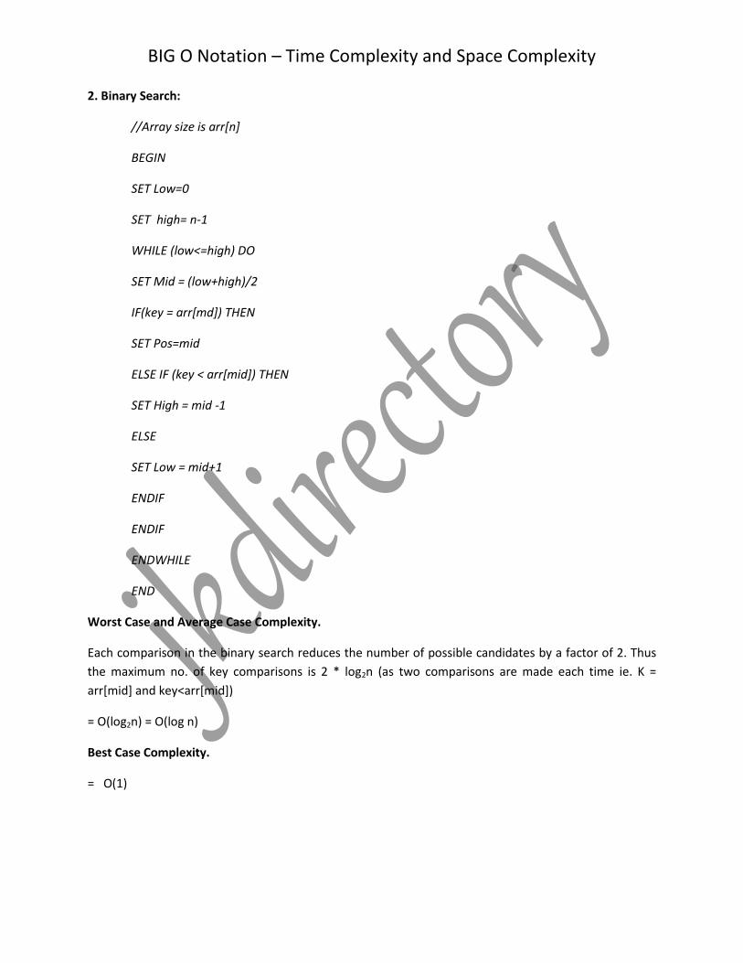
2. Binary Search:

//Array size is arr[n]

BEGIN

SET Low=0

SET high= n-1

WHILE (low<=high) DO

SET Mid = (low+high)/2

IF(key = arr[md]) THEN

SET Pos=mid

ELSE IF (key < arr[mid]) THEN

SET High = mid -1

ELSE

SET Low = mid+1

ENDIF

ENDIF

ENDWHILE

END

Worst Case and Average Case Complexity.

Each comparison in the binary search reduces the number of possible candidates by a factor of 2. Thus

the maximum no. of key comparisons is 2 * log2n (as two comparisons are made each time ie. K =

arr[mid] and key<arr[mid])

= O(log2n) = O(log n)

Best Case Complexity.

= O(1)


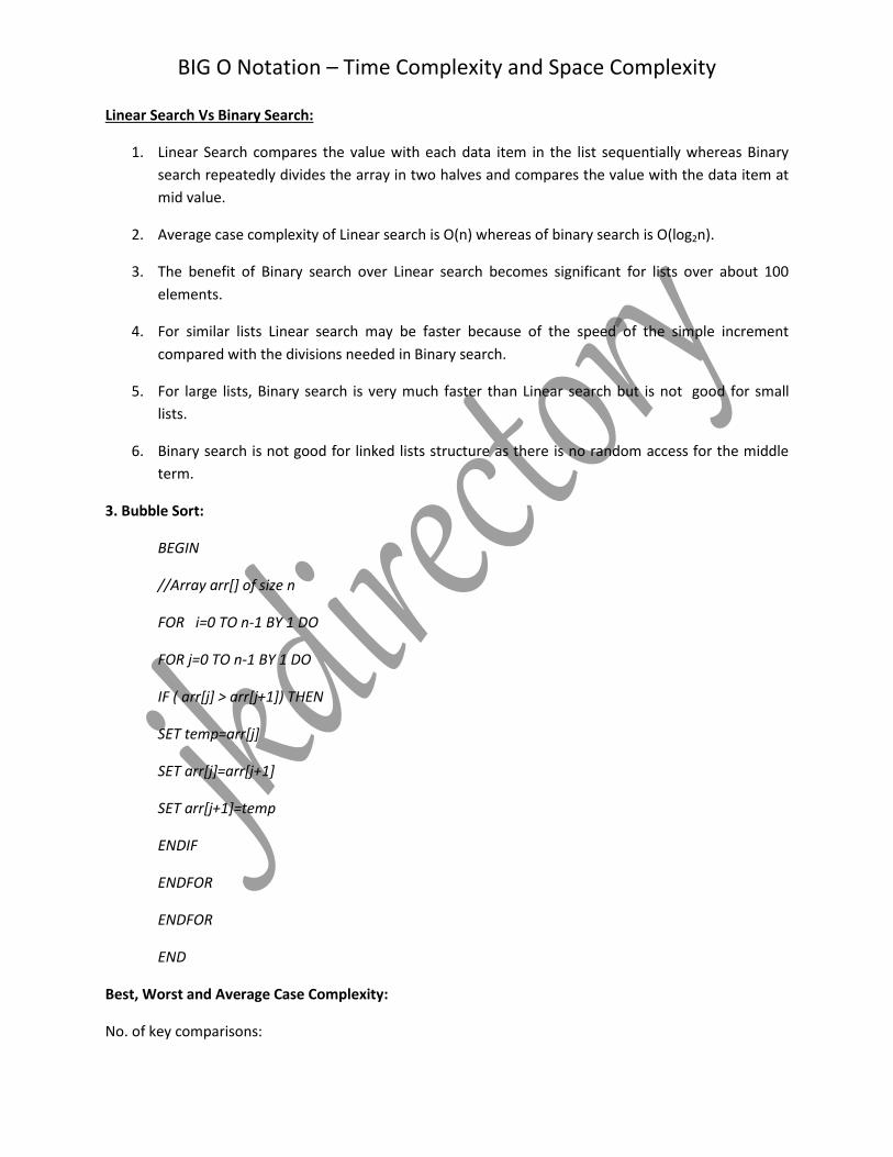
Linear Search Vs Binary Search:

1. Linear Search compares the value with each data item in the list sequentially whereas Binary

search repeatedly divides the array in two halves and compares the value with the data item at

mid value.

2. Average case complexity of Linear search is O(n) whereas of binary search is O(log2n).

3. The benefit of Binary search over Linear search becomes significant for lists over about 100

elements.

4. For similar lists Linear search may be faster because of the speed of the simple increment

compared with the divisions needed in Binary search.

5. For large lists, Binary search is very much faster than Linear search but is not good for small

lists.

6. Binary search is not good for linked lists structure as there is no random access for the middle

term.

3. Bubble Sort:

BEGIN

//Array arr[] of size n

FOR i=0 TO n-1 BY 1 DO

FOR j=0 TO n-1 BY 1 DO

IF ( arr[j] > arr[j+1]) THEN

SET temp=arr[j]

SET arr[j]=arr[j+1]

SET arr[j+1]=temp

ENDIF

ENDFOR

ENDFOR

END

Best, Worst and Average Case Complexity:

No. of key comparisons:


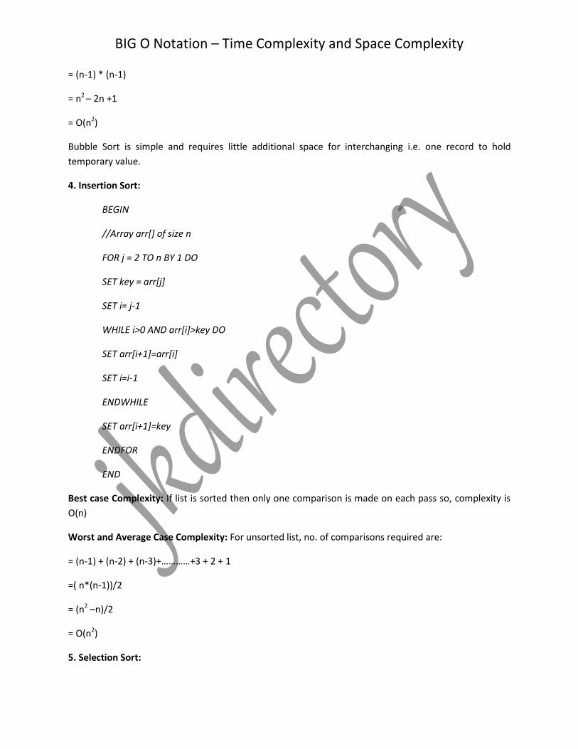
= (n-1) * (n-1)

= n2 – 2n +1

= O(n2)

Bubble Sort is simple and requires little additional space for interchanging i.e. one record to hold

temporary value.

4. Insertion Sort:

BEGIN

//Array arr[] of size n

FOR j = 2 TO n BY 1 DO

SET key = arr[j]

SET i= j-1

WHILE i>0 AND arr[i]>key DO

SET arr[i+1]=arr[i]

SET i=i-1

ENDWHILE

SET arr[i+1]=key

ENDFOR

END

Best case Complexity: If list is sorted then only one comparison is made on each pass so, complexity is

O(n)

Worst and Average Case Complexity: For unsorted list, no. of comparisons required are:

= (n-1) + (n-2) + (n-3)+…………+3 + 2 + 1

=( n*(n-1))/2

= (n2 –n)/2

= O(n2)

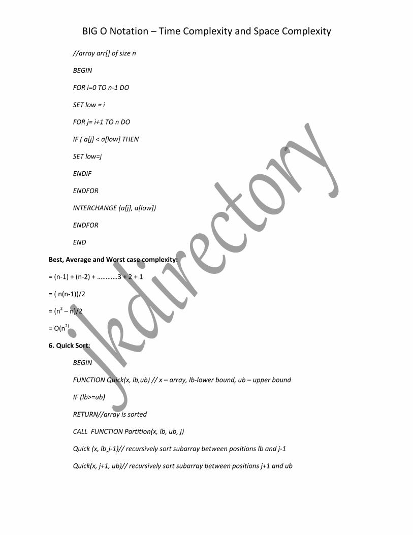
5. Selection Sort:


//array arr[] of size n

BEGIN

FOR i=0 TO n-1 DO

SET low = i

FOR j= i+1 TO n DO

IF ( a[j] < a[low] THEN

SET low=j

ENDIF

ENDFOR

INTERCHANGE (a[j], a[low])

ENDFOR

END

Best, Average and Worst case complexity:

= (n-1) + (n-2) + …………3 + 2 + 1

= ( n(n-1))/2

= (n2 – n)/2

= O(n2)

6. Quick Sort:

BEGIN

FUNCTION Quick(x, lb,ub) // x – array, lb-lower bound, ub – upper bound

IF (lb>=ub)

RETURN//array is sorted

CALL FUNCTION Partition(x, lb, ub, j)

Quick (x, lb¸j-1)// recursively sort subarray between positions lb and j-1

Quick(x, j+1, ub)// recursively sort subarray between positions j+1 and ub


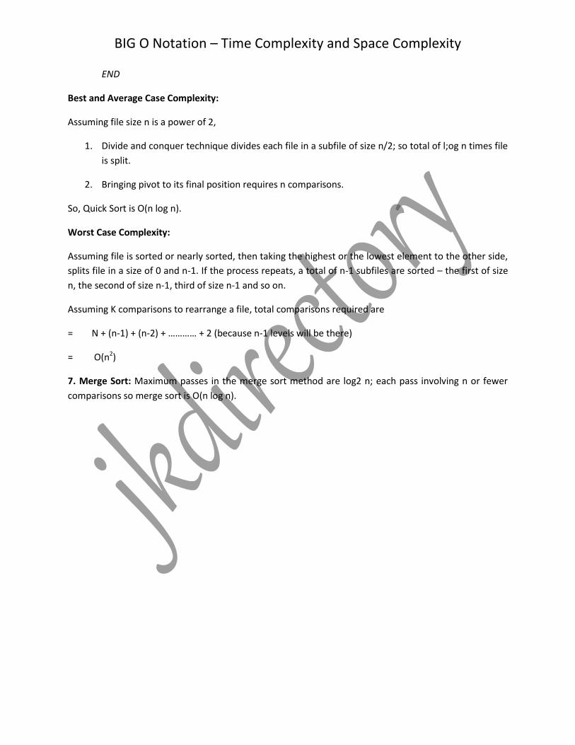
END

Best and Average Case Complexity:

Assuming file size n is a power of 2,

1. Divide and conquer technique divides each file in a subfile of size n/2; so total of l;og n times file

is split.

2. Bringing pivot to its final position requires n comparisons.

So, Quick Sort is O(n log n).

Worst Case Complexity:

Assuming file is sorted or nearly sorted, then taking the highest or the lowest element to the other side,

splits file in a size of 0 and n-1. If the process repeats, a total of n-1 subfiles are sorted – the first of size

n, the second of size n-1, third of size n-1 and so on.

Assuming K comparisons to rearrange a file, total comparisons required are

= N + (n-1) + (n-2) + ………… + 2 (because n-1 levels will be there)

= O(n2)

7. Merge Sort: Maximum passes in the merge sort method are log2 n; each pass involving n or fewer

comparisons so merge sort is O(n log n).

Documents

BIG O Notation Time Complexity and Space Complexity · BIG O Notation – Time Complexity and Space Complexity ... Conditional checks: ... Time Complexity and Space Complexity ) )