BIOEN 482 Senior Capstone Thesis

7/28/2019 BIOEN 482 Senior Capstone Thesis

http://slidepdf.com/reader/full/bioen-482-senior-capstone-thesis 1/49

Three-Dimensional Modeling

of the Osteocyte Network

by

Chao Huang

Advisor: Ted S. Gross, Ph.D.

University of Washington

Department of Bioengineering

Senior Capstone Project

6 June 2008



Table of Contents

ABSTRACT ................................................................................................................................ 2

INTRODUCTION...................................................................................................................... 3

DEFINITION OF PROJECT ............................................................................................................... 3MEDICAL AND SCIENTIFIC SIGNIFICANCE ..................................................................................... 4SOCIAL, ETHICAL, AND ECONOMIC ISSUES.................................................................................... 5TECHNICAL BACKGROUND ........................................................................................................... 7

Theory ..................................................................................................................................... 7 Review of literature................................................................................................................. 9 Previous relevant work in advisor’s laboratory ................................................................... 14 Outstanding technical issues at outset of project ................................................................. 17

INITIAL DESIGN OF EXPERIMENTS, TOOLS, AND DEVICES........................ 19 MATERIALS AND METHODS ........................................................................................................ 19COSTS ........................................................................................................................................ 26I NITIAL RESEARCH PLAN ............................................................................................................ 27

RESULTS.................................................................................................................................. 29

FINAL TIMELINE ......................................................................................................................... 29DATA ......................................................................................................................................... 30EXPERIMENTAL/DESIGN DECISIONS............................................................................................ 38A NALYSIS AND CONCLUSIONS.................................................................................................... 39SUGGESTIONS FOR FUTURE WORK .............................................................................................. 43

ACKNOWLEDGEMENTS.................................................................................................... 45

REFERENCES......................................................................................................................... 46

1



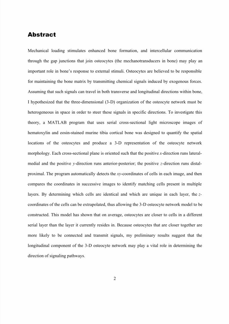
Abstract

Mechanical loading stimulates enhanced bone formation, and intercellular communication

through the gap junctions that join osteocytes (the mechanotransducers in bone) may play an

important role in bone’s response to external stimuli. Osteocytes are believed to be responsible

for maintaining the bone matrix by transmitting chemical signals induced by exogenous forces.

Assuming that such signals can travel in both transverse and longitudinal directions within bone,

I hypothesized that the three-dimensional (3-D) organization of the osteocyte network must be

heterogeneous in space in order to steer these signals in specific directions. To investigate this

theory, a MATLAB program that uses serial cross-sectional light microscope images of

hematoxylin and eosin-stained murine tibia cortical bone was designed to quantify the spatial

locations of the osteocytes and produce a 3-D representation of the osteocyte network

morphology. Each cross-sectional plane is oriented such that the positive x-direction runs lateral-

medial and the positive y-direction runs anterior-posterior; the positive z-direction runs distal-

proximal. The program automatically detects the xy-coordinates of cells in each image, and then

compares the coordinates in successive images to identify matching cells present in multiple

layers. By determining which cells are identical and which are unique in each layer, the z-

coordinates of the cells can be extrapolated, thus allowing the 3-D osteocyte network model to be

constructed. This model has shown that on average, osteocytes are closer to cells in a different

serial layer than the layer it currently resides in. Because osteocytes that are closer together are

more likely to be connected and transmit signals, my preliminary results suggest that the

longitudinal component of the 3-D osteocyte network may play a vital role in determining the

direction of signaling pathways.

2



Introduction

Definition of project

There is a need to develop a simple and fast method for identifying the three-dimensional (3-D)

locations of osteocytes within a piece of bone. I have designed a MATLAB program that uses

serial transverse images to automatically construct a 3-D model of the osteocyte network in

murine cortical bone. The program takes the images as inputs and automatically detects the

osteocyte locations in each cross-section through filtering means. A graphical user interface is

provided to allow the user to manually correct any mistakes that the program has made in

detecting cell locations. The user enters the current layer number for each cross-section in the

ordered series of images, and saves this information along with the xy-coordinates as separate

MATLAB files that can be loaded and accessed later. Once the necessary coordinate information

has been collected for each image, the user may then choose the desired files to be used to

construct the network model (the files must be contiguous cross-sections and in order).

The model is a 3-D scatterplot that shows the spatial locations of the osteocytes in the

user-selected layers and may be rotated in any direction to provide many different views. Upon

saving the model, the user may select a number of parameters to be calculated, including the

number of cells in each layer, the number cells in predefined sectors of each cross-section (to

determine uniformity), and the minimum distance between neighboring cells for both planar and

z-directions. Being able to perform morphological analysis by quantifying the 3-D organization

of osteocytes within the section of bone is an important step for tracing the direction of their

signaling pathways.

3



Medical and scientific significance

In humans, cortical (outer layer) and trabecular (spongy bone within the joint ends) bone begin to

degrade after peak bone mass is reached at approximately 30 years of age [6]. This degradation

is the result of elevated bone resorption (breakdown of bone and release of minerals) and

decreased bone formation [3]. By age 40, bone loss is estimated to be 0.3% to 0.5% per year, and

in women, menopause may elevate annual bone loss to up to 3% [6]. Based on these estimates,

an average 70-year-old woman may experience a decrease of 25% to up to 40% in bone mass

from her peak bone mass while a like-aged man may expect a decline of 10% to 15% [7]. In

addition, diseases such as osteoporosis may further reduce the bone mineral density, therefore

increasing the risk of bone fracture and posing a significant health concern for senior citizens [8].

Given these concerns, it is essential to develop novel techniques for sustaining or augmenting

bone mass throughout an individual’s lifetime.

One of the signals for bone cells to form new bones is mechanical stress, such as that

experienced during exercise [9]. Previous studies have shown that bone mass increases with

exercise, and so it is apparent that mechanical components of bone’s functional environment

have an effect on bone mass and morphology [10]. By studying how loads are anabolic to bone

and identifying specific signals responsible for inducing new bone formation, non-

pharmacologic methods using mechanical loading may be developed to inhibit osteoporosis and

promote osteogenesis [11].

A model of the osteocyte network in bone must be constructed in order to visualize where

bone cells are in relation to each other and understand how their organization dictates the

transmission of mechanical signals to induce bone formation. As will be highlighted in the

proceeding literature review, previous methods for analyzing signaling pathways in osteocyte

4



networks have either focused on osteocytes in a two-dimensional plane or used complicated and

expensive techniques and equipment to construct a three-dimensional (3-D) model. Thus, there is

a need to design a simple, easy, and fast computer program that will find the 3-D locations of

osteocytes fairly accurately and perform basic morphological analysis in a short amount of time.

Although there are already 3-D reconstruction programs available (e.g. ImageJ), such programs

do not offer the same capabilities of a program designed specifically for analysis of a network of

cells within bone. For example, traditional imaging methods would require the user to manually

locate where cells are, which is both laborious and time-consuming. The program that I have

designed automatically finds the locations of cells, constructs the 3-D model, and then performs

calculations related to the organization of the network of cells. Gathering such data will yield

substantial insight into how osteocytes are organized in bone and how the architecture of these

networks might play a role in the complex process of bone formation in response to mechanical

loading. Constructing an accurate model of the osteocyte network is therefore essential for

tracing the mechanotransduction signaling pathways that induce bone growth.

Social, ethical, and economic issues

Bone formation induced by mechanical stress is studied with the ultimate goal of adapting and

using mechanical loading in a clinical setting. If the ways in which bone perceives and responds

to mechanical stimuli are well understood, then such information may be used to design novel

exercise regimens that provoke a similar response in bone as mechanical loading. Exercise is a

socially accepted activity in all cultures of the world that is widely considered to promote good

health. Therefore, it is not expected that introducing a new exercise regimen specially designed

to induce bone growth will engender substantial fear or mistrust among the public. While the

public may be much more hesitant to use a new device or undergo a surgical procedure, a novel

5



exercise regimen should not be a difficult medical technique to encourage the public to try.

Previous studies have shown that athletes who play racquet sports have enhanced bone mass in

their serving arms [12], and these visible and tangible results should encourage subjects to

choose exercise over other pharmacological means of inducing bone formation.

Because exercise regimens present a non-pharmacological intervention for bone loss, it is

also expected that such treatments will not be as difficult to gain FDA approval for as

pharmaceutical treatments such as estrogens and bisphophonates. In addition, when the

biochemistry and mechanics of bone formation are better understood, exercise regimens will be

specially designed for the elderly to induce maximal bone formation from minimal strain

magnitudes, lessening any ethical concern for causing injury during clinical trials. Furthermore,

it may be more beneficial socially and ethically for the public to adopt a non-pharmacological

technique for enhancing bone formation since it is a tangible activity that can be controlled by

the individual, unlike reading directions and blindly taking medication without knowing what is

happening inside one’s body.

A final advantage of mechanically induced bone formation over pharmacological

treatments is that, beyond experimental and clinical testing, there is little to no cost involved. In

1995, the national healthcare cost of osteoporosis was estimated to be $13.8 billion and may

increase to as much as $240 billion over the next 50 years [13]. Most of these costs can be

attributed to either medication, which may be avoided if the exercise alternative is chosen, or

surgery, which may also be avoided if individuals begin their exercise regimens earlier in life.

With the potential social, ethical, and economic benefits of a possible low-magnitude exercise

regimen, mechanical loading holds the potential to be an effective and safe technique for

inducing new bone formation to counter the effects of aging.

6



Technical background

Theory

The primary mechanical function of bone is to provide support for muscles to act against and

hold the body in an upright position [14]. Bone is constantly subjected to a dynamic loading

environment through a person’s daily movements, and therefore must adapt responsively to

maintain its structure and withstand physical activity [15]. The basis for bone’s adaptation to

exogenous forces is through bone remodeling, which consists of bone resorption and new bone

formation. Bone resorption is the breaking down of bone into its minerals (such as calcium) by

osteoclasts, resulting in the transfer of such minerals and proteins to a different location via

blood [16]. New bone is then formed by osteoblasts that synthesize osteoid, an unmineralized

bone matrix composed of organic components. Some osteoblasts will become trapped within the

matrix that they lay down and differentiate into osteocytes, the most abundant cells in bone (each

spanning approximately 10 μm) [17]. In addition to being responsible for maintaining the bone

matrix, osteocytes are believed to be the mechanosensors and mechanotransducers in bone [18].

Bone adaptation requires cellular mechanotransduction, and osteocytes are affected by a

variety of mechanical factors generated by loading. These factors include strain generated across

the cells’ substrate, pressure within intramedullary cavities, and shear forces through the

canaliculi that connect the cells [11]. The conversion of these forces into a cellular response

consists of four phases: mechanocoupling, biochemical coupling, transmission of signaling, and

effector cell response. During mechanocoupling, the applied mechanical forces are transduced

into local mechanical signals perceived by osteocytes [14]. Such signals may be sensed by a

number of mechanoreceptors including mechanosensitive channels that induce membrane hyper

or depolarization, integrin proteins that span the membrane to couple the cell to its extracellular

environment, connexins that form regulated channels allowing direct exchange of small

7



molecules between adjacent cells, and membrane structure proteins that facilitate transmembrane

communication as well as provide docking positions for signaling complexes [11]. After these

local mechanical signals are sensed, biochemical coupling occurs, when the mechanical signals

are transduced into biochemical signals that lead to gene expression or protein activation [14].

Biochemical signaling may occur through G-proteins, calcium transients, MAPK activation, and

release of nitric oxide [11].

Cell-to-cell transmission of biochemical signals occurs intracellularly through the

processes that join osteocytes as well as through the extracellular fluid in which osteocytes are

immersed [19]. Gap junctions at the tip of the cell processes that contain hemichannels provide a

direct and efficient mechanism for intracellular signaling pathways [20], although osteocytes also

remain in contact via their common environment in the contiguous bone fluid space. Such fluid

acts as a coupling medium through which mechanochemical signals may still be transmitted by

hydraulic conductivity, pressure and osmotic gradients, as well as electromechanical and

acoustic energy effects [15]. The combination of the intracellular and extracellular transmission

of signals induces an effector cell response at the tissue level, at which point bone remodeling

commences [14].

The degree of bone adaptation in response to external loading depends on strain

magnitude, distribution, duration, frequency, bone history, and type of stress created

(compression, tension, or shear). Over the last century, numerous experiments have been

conducted to test each of these factors’ effect on bone adaptation and many common threads

have emerged [21]. The following literature review highlights some of these findings and ends

with a summary of the research on bone adaptation being carried out in my current advisor’s

laboratory.

8



Review of literature

The notion that the form and function of bone is produced and maintained by mechanical forces

was first popularized by anatomist Julius Wolff in his 1892 treatise, The Law of Bone

Remodeling [22]. In what has now become known as Wolff’s Law, Wolff states that “Every

change in the form and function of bone […] is followed by certain definite changes in their

internal architecture, and equally definite alteration in their external conformation, in accordance

with mathematical laws [23].” Through demonstrating a definite link between trabecular bone

architecture and the functional stresses placed upon it, Wolff was able to assert that the stresses

surrounding bone forces the architecture inside living bone to continuously adapt through

remodeling. Later, embryologist Wilhelm Roux generalized the notion of functional adaptation,

suggesting that mechanical stimuli govern effector cells that regulate bone’s formation and

adaptation locally in a self-organizational process [22]. In the early 20th Century, biologist

D’arcy Thompson proposed that the condition of strain, caused by the stress induced by

mechanical forces, is a direct stimulus for bone growth and thus is the source of functional

adaptation. In the 1960’s, orthopedist Harold Frost asserted that not only was mechanical strain

the primary determinant of bone adaptation, but that a minimum strain threshold must be reached

before bone adaptation occurs [21]. The combination of all these findings provided a foundation

for other investigators to study the relationship between bone’s mechanical environment and its

effect on bone’s development of mass and architecture.

Early investigations that have used approaches such as exercise, disuse, and stress

protection employed loading regimens superimposed on existing effects of normal load-bearing,

and thus an accurate, discernable remodeling response to the newly applied mechanical situation

could not be extracted [1]. Such difficulties led to the design of novel experimental setups that

could elucidate bone’s functional adaptation to mechanical forces. A new technique in which

9



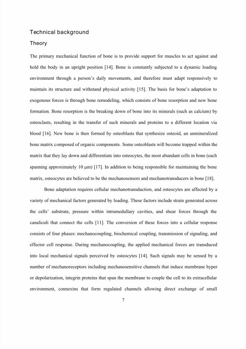
bones were externally loaded in vivo over a period

of weeks was first used by Hert et al. in early

1970’s studies with rabbits. Hert found that dynamic

strains increased the amount of bone formation in

the rabbits while static strains did not, and therefore

suggested that dynamic strains are primarily

responsible for bone adaptation [21]. In 1984,

Rubin and Lanyon refined Hert’s loading approach and confirmed his findings by functionally

isolating the external ulnae in turkeys and applying known intermittent loads over a period of six

weeks. As Figure 1 illustrates, a template was clamped and pinned to the ulna, allowing two

parallel transverse osteotomies to be performed and leaving the entire midshaft of the ulna

undisturbed. The ends of the pins were connected to a loading apparatus that imposed a 0.5-Hz

intermittent compressive load cycle to engender strains in the bone. The number of consecutive

load cycles that was applied each day was varied to determine the bone’s response to different

load magnitudes. The strains were measured at the surface of the bone using strain gauges and

could be directly correlated to the remodeling induced by the loading. Photon-absorption

densitometry and postmortem histological methods were used to comparatively assess bone

mineral content and determine the course of remodeling in response to the strain stimulus [1].

Figure 1: Schematic of template used for parallel osteotomies and holding the ulna in place as loads were administered [1].

In comparisons of unloaded, control bone and dynamically loaded bone with a variable

number of consecutive load cycles, it was found that bone mass decreased in ulnae that were not

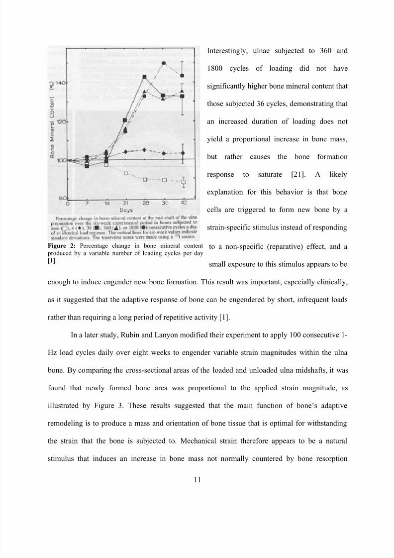
subjected to any external loading, which was the predicted response to disuse. As Figure 2

shows, ulnae subjected to four loading cycles a day showed a slight increase in bone mineral

content, and as the number of consecutive cycles was increased to 36 cycles of an identical strain

regimen, substantial subperiosteal and endosteal new-bone formation was measured [1].

10



Interestingly, ulnae subjected to 360 and

1800 cycles of loading did not have

significantly higher bone mineral content that

those subjected 36 cycles, demonstrating that

an increased duration of loading does not

yield a proportional increase in bone mass,

but rather causes the bone formation

response to saturate [21]. A likely

explanation for this behavior is that bone

cells are triggered to form new bone by a

strain-specific stimulus instead of responding

to a non-specific (reparative) effect, and a

small exposure to this stimulus appears to be

enough to induce engender new bone formation. This result was important, especially clinically,

as it suggested that the adaptive response of bone can be engendered by short, infrequent loads

rather than requiring a long period of repetitive ac

Figure 2: Percentage change in bone mineral content produced by a variable number of loading cycles per day[1].

tivity [1].

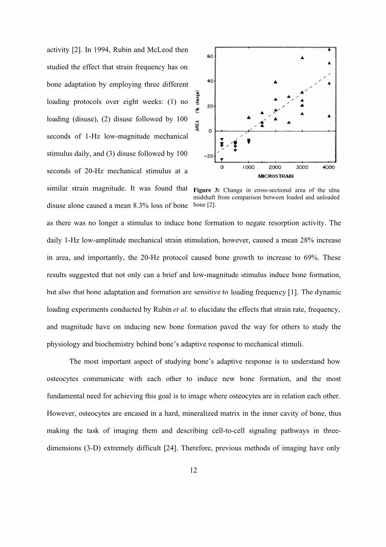
In a later study, Rubin and Lanyon modified their experiment to apply 100 consecutive 1-

Hz load cycles daily over eight weeks to engender variable strain magnitudes within the ulna

bone. By comparing the cross-sectional areas of the loaded and unloaded ulna midshafts, it was

found that newly formed bone area was proportional to the applied strain magnitude, as

illustrated by Figure 3. These results suggested that the main function of bone’s adaptive

remodeling is to produce a mass and orientation of bone tissue that is optimal for withstanding

the strain that the bone is subjected to. Mechanical strain therefore appears to be a natural

stimulus that induces an increase in bone mass not normally countered by bone resorption

11



activity [2]. In 1994, Rubin and McLeod then

studied the effect that strain frequency has on

bone adaptation by employing three different

loading protocols over eight weeks: (1) no

loading (disuse), (2) disuse followed by 100

seconds of 1-Hz low-magnitude mechanical

stimulus daily, and (3) disuse followed by 100

seconds of 20-Hz mechanical stimulus at a

similar strain magnitude. It was found that

disuse alone caused a mean 8.3% loss of bone

as there was no longer a stimulus to induce bone formation to negate resorption activity. The

daily 1-Hz low-amplitude mechanical strain stimulation, however, caused a mean 28% increase

in area, and importantly, the 20-Hz protocol caused bone growth to increase to 69%. These

results suggested that not only can a brief and low-magnitude stimulus induce bone formation,

but also that bone adaptation and formation are sensitive to loading frequency [1]. The dynamic

loading experiments conducted by Rubin et al. to elucidate the effects that strain rate, frequency,

and magnitude have on inducing new bone formation paved the way for others to study the

physiology and biochemistry behind bone’s adaptive response to mechanical stimuli.

Figure 3: Change in cross-sectional area of the ulnamidshaft from comparison between loaded and unloaded bone [2].

The most important aspect of studying bone’s adaptive response is to understand how

osteocytes communicate with each other to induce new bone formation, and the most

fundamental need for achieving this goal is to image where osteocytes are in relation each other.

However, osteocytes are encased in a hard, mineralized matrix in the inner cavity of bone, thus

making the task of imaging them and describing cell-to-cell signaling pathways in three-

dimensions (3-D) extremely difficult [24]. Therefore, previous methods of imaging have only

12



been capable of showing the osteocyte distribution in a two-dimensional (2-D) plane. For

example, Krempien et al. revealed the non-viable cell network in 2-D by staining lacunae (small

spaces in the bone that contain one osteocyte each) with fuchsin stain [25]. Such a network

model is not sufficient for analyzing the direction of signaling pathways as the longitudinal

component along the length of the bone is not included.

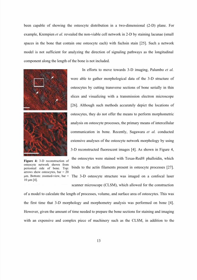
In efforts to move towards 3-D imaging, Palumbo et al.

were able to gather morphological data of the 3-D structure of

osteocytes by cutting transverse sections of bone serially in thin

slices and visualizing with a transmission electron microscope

[26]. Although such methods accurately depict the locations of

osteocytes, they do not offer the means to perform morphometric

analysis on osteocyte processes, the primary means of intercellular

communication in bone. Recently, Sugawara et al. conducted

extensive analyses of the osteocyte network morphology by using

3-D reconstructed fluorescent images [4]. As shown in Figure 4,

the osteocytes were stained with Texas-Red® phalloidin, which

binds to the actin filaments present in osteocyte processes [27].

The 3-D osteocyte structure was imaged on a confocal laser

scanner microscope (CLSM), which allowed for the construction

of a model to calculate the length of processes, volume, and surface area of osteocytes. This was

the first time that 3-D morphology and morphometry analysis was performed on bone [4].

However, given the amount of time needed to prepare the bone sections for staining and imaging

with an expensive and complex piece of machinery such as the CLSM, in addition to the

Figure 4: 3-D reconstruction of osteocyte network shown from periosteal side of bone. Top:arrows show osteocytes, bar = 20

μm. Bottom: zoomed-view, bar =

10 μm [4].

13



laborious task of manually collecting morphological data, it is evident that there is a need to

develop a simpler and faster way of analyzing the 3-D osteocyte network.

Previous relevant work in advisor’s laboratory

The laboratory group that I have joined, the

Orthopaedics Science Laboratories (OSL)

directed by Professor Ted S. Gross, examines

how bone responds to physical stimuli. Many of

the aforementioned methods for loading and

imaging have been adapted for investigation and

modeling of real-time cell-to-cell signaling in

response to mechanical loading.

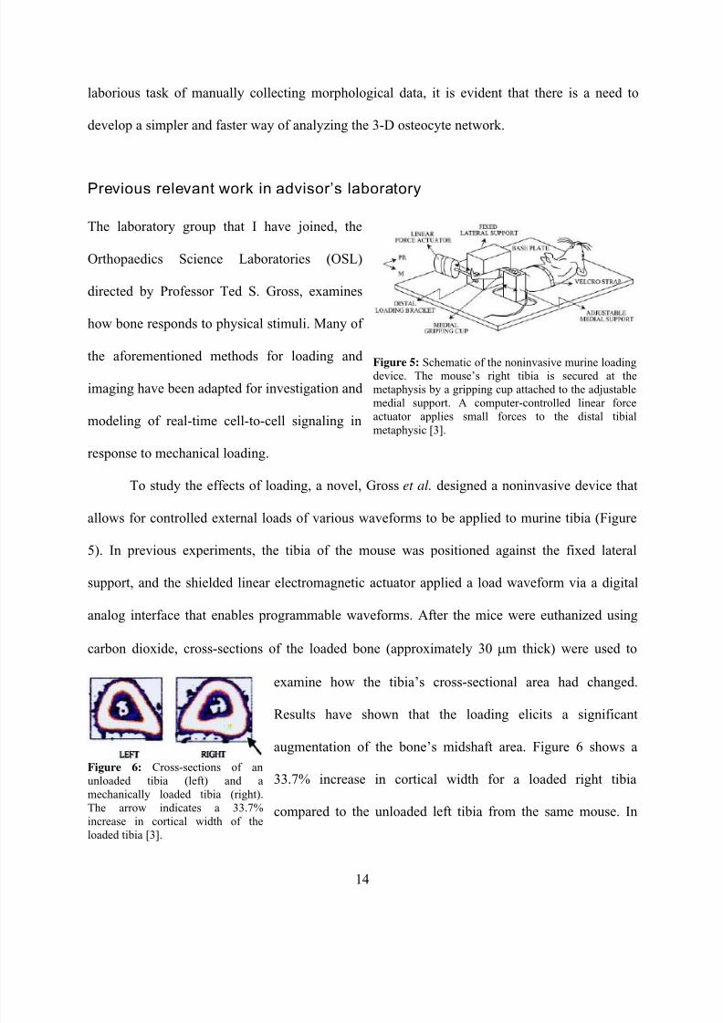
Figure 5: Schematic of the noninvasive murine loadingdevice. The mouse’s right tibia is secured at themetaphysis by a gripping cup attached to the adjustablemedial support. A computer-controlled linear forceactuator applies small forces to the distal tibialmetaphysic [3].

To study the effects of loading, a novel, Gross et al. designed a noninvasive device that

allows for controlled external loads of various waveforms to be applied to murine tibia (Figure

5). In previous experiments, the tibia of the mouse was positioned against the fixed lateral

support, and the shielded linear electromagnetic actuator applied a load waveform via a digital

analog interface that enables programmable waveforms. After the mice were euthanized using

carbon dioxide, cross-sections of the loaded bone (approximately 30 μm thick) were used to

examine how the tibia’s cross-sectional area had changed.

Results have shown that the loading elicits a significant

.7% increase in cortical width for a loaded right tibia

ompared to the unloaded left tibia from the same mouse. In

augmentation of the bone’s midshaft area. Figure 6 shows a

33

c

Figure 6: Cross-sections of anunloaded tibia (left) and amechanically loaded tibia (right).The arrow indicates a 33.7%increase in cortical width of theloaded tibia [3].

14



addition, Gross et al. confirmed Rubin and Lanyon’s observation that dynamic loading induced

substantial new bone formation whereas static loading produced an absence of response. It was

concluded that the mechanical loading device is capable of noninvasively inducing an anabolic

response to mechanical load consistent with aforementioned models of bone adaptation [3].

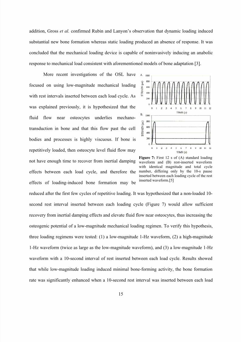
More recent investigations of the OSL have

focused

not have enough time to recover from inertial damping

at a non-loaded 10-

on using low-magnitude mechanical loading

with rest intervals inserted between each load cycle. As

was explained previously, it is hypothesized that the

fluid flow near osteocytes underlies mechano-

transduction in bone and that this flow past the cell

bodies and processes is highly viscuous. If bone is

repetitively loaded, then osteocyte level fluid flow may

effects between each load cycle, and therefore the

effects of loading-induced bone formation may be

reduced after the first few cycles of repetitive loading. It w

second rest interval inserted between each loading cycle (Figure 7) would allow sufficient

recovery from inertial damping effects and elevate fluid flow near osteocytes, thus increasing the

osteogenic potential of a low-magnitude mechanical loading regimen. To verify this hypothesis,

three loading regimens were tested: (1) a low-magnitude 1-Hz waveform, (2) a high-magnitude

1-Hz waveform (twice as large as the low-magnitude waveform), and (3) a low-magnitude 1-Hz

waveform with a 10-second interval of rest inserted between each load cycle. Results showed

that while low-magnitude loading induced minimal bone-forming activity, the bone formation

rate was significantly enhanced when a 10-second rest interval was inserted between each load

Figure 7: First 12 s of (A) standard loadingwaveform and (B) rest-inserted waveformwith identical magnitude and total cyclenumber, differing only by the 10-s pauseinserted between each loading cycle of the rest

inserted waveform.[5]

as hypothesized th

15



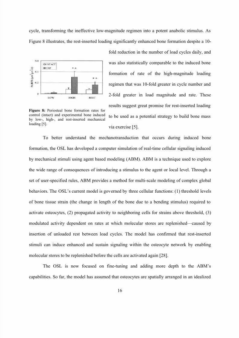
cycle, transforming the ineffective low-magnitude regimen into a potent anabolic stimulus. As

Figure 8 illustrates, the rest-inserted loading significantly enhanced bone formation despite a 10-

fold reduction in the number of load cycles daily, and

was also statistically comparable to the induced bone

formation of rate of the high-magnitude loading

regimen that was 10-fold greater in cycle number and

2-fold greater in load magnitude and rate. These

results suggest great promise for rest-inserted loading

to be used as a potential strategy to build bone mass

via exercise [5].

anotransduction that occurs during induced bone

formation, the OS

Figure 8: Periosteal bone formation rates for control (intact) and experimental bone induced

by low-, high-, and rest-inserted mechanicalloading [5].

To better understand the mech

L has developed a computer simulation of real-time cellular signaling induced

by mec

nged in an idealized

hanical stimuli using agent based modeling (ABM). ABM is a technique used to explore

the wide range of consequences of introducing a stimulus to the agent or local level. Through a

set of user-specified rules, ABM provides a method for multi-scale modeling of complex global

behaviors. The OSL’s current model is governed by three cellular functions: (1) threshold levels

of bone tissue strain (the change in length of the bone due to a bending stimulus) required to

activate osteocytes, (2) propagated activity to neighboring cells for strains above threshold, (3)

modulated activity dependent on rates at which molecular stores are replenished––caused by

insertion of unloaded rest between load cycles. The model has confirmed that rest-inserted

stimuli can induce enhanced and sustain signaling within the osteocyte network by enabling

molecular stores to be replenished before the cells are activated again [28].

The OSL is now focused on fine-tuning and adding more depth to the ABM’s

capabilities. So far, the model has assumed that osteocytes are spatially arra

16



networ

hnical issues at outset of pro ject

my original capstone proposal, I aimed to not only find the 3-D locations of the osteocyte

er processes. I proposed to use a

k within cortical bone [28]. Thus, the model would be greatly improved if a more accurate

description of where exactly osteocytes are located within a volume of bone was provided. My

project makes it possible for the 3-D locations of osteocytes to be found automatically and

quickly, therefore introducing the opportunity of incorporating this 3-D network of cells into the

ABM simulations.

Outstanding tec

In

bodies, but also show the interconnectivity of their long, slend

confocal laser scanning microscope to image bone sections stained with the fluorescent

phallotoxin phalloidin that binds at the interface between F-actin subunits in the osteocyte

processes [29], much like Sugawara et al.’s method described previously [4]. However, when

using the Differential Interference Contrast mode on the confocal laser scanning microscope

(CLSM), I found the fluorescent stain was not concentrated in the osteocyte cell bodies, but

rather was spread out throughout all regions of the imaging plane. I concluded that this result

must suggest that the phalloidin was not binding specifically to the actin in osteocytes, and

proceeded to spend the majority of the Summer and Autumn quarters of 2007 altering and testing

my staining protocol. After employing many changes that still did not produce improved images,

I contacted Invitrogen (the company that supplied the phalloidin) for product support. Invitrogen

suggested that the reason why the phalloidin was non-specifically binding the osteocytes is

because the actin filaments in the processes were being denatured by the incubation step in my

procedure, and recommended that I try cryo-sectioning instead. After considering the amount of

work left to finish and the decreasing amount of time left, I decided that attempting to learn, use,

and potentially still be unsuccessful with cryo-sectioning was not an idea worth pursuing.

17



Therefore, I settled on using light microscopy to image my bone sections with hematoxylin and

eosin (H&E) staining, a simpler and faster protocol that the OSL had had success with in the

past.

Hematoxylin is a dye that colors basophilic structures containing nucleic acids blue while

the alcohol-based acidic eosin is a dye that colors eosinophilic structures composed of

intracellular or extracellular protein pink. Thus, in a bone-cross section, the nuclei of the

osteocytes would appear as blue while its surrounding regions would appear pink, allowing the

locations of the cells to be easily seen [30]. The disadvantage of using H&E stain is that it is not

fluorescent and thus incompatible with the CLSM. Using the z-motor feature of the CLSM, serial

transverse images could be taken at predetermined intervals of a thick section of bone stained

with phalloidin. With H&E and light microscopy, however, these individual thin transverse

sections must be physically cut in order to be stained and imaged. Such a procedure creates an

image registration problem, as each imaged section will be misaligned relative to others, thus

creating difficulties in comparing the coordinates of osteocyte locations between sections.

Addressing this technical issue was the main challenge in writing my MATLAB program for

creating the 3-D osteocyte network model, and the design process is detailed in the proceeding

Methods section.

18



Initial Design of Experiments, Tools, and Devices

Materials and methods

A section of bone taken from the midshaft of an unloaded (control) left murine tibia was

decalcified and embedded in paraffin blocks. Five serial transverse sections, each 5 μm thick,

were machine-cut from the block, mounted on glass slides, and stained with a commercially

available hematoxylin dye and a prepared eosin solution following the proceeding protocol. A

stock solution of eosin was made from 1 g Eosin Y dye, 20 mL deionized water, and 80 mL 95%

ethanol (EtOH), and the working solution of eosin was made from 25 mL stock solution, 75 mL

80% EtOH, and 0.5 mL Glacial Acetic Acid.

H&E Staining Protocol for Paraffin-Embedded Sections

1. De-paraffinization and rehydrationa. Wash in 3 changes of xylene (5 min. each). Blot excess xylene. b. Wash in 100% EtOH (5 min.)c. Wash in 95% EtOH (3 min.)

d.

Wash in 80% EtOH (3 min.)e. Wash in 70% EtOH (3 min.)f. Wash in deionized water (5 min.)

2. Hematoxylin staininga. Stain with hematoxylin (5 min.) b. Wash in tap water to allow stain to develop (5 min.)c. Wash in deionized water (5 min.). Blot excess water.

3. Eosin staining and dehydrationa. Stain with eosin working solution (30 sec.) b. Wash in 70% EtOH (5 min.)c. Wash in 2 changes of 95% EtOH (1 min. each)d. Wash in 2 changes of 100% EtOH (3 min. each). Blot excess EtOH.e. Wash in xylene (15 min.)

4. Coverslip slides using Permount (xylene-based).

19



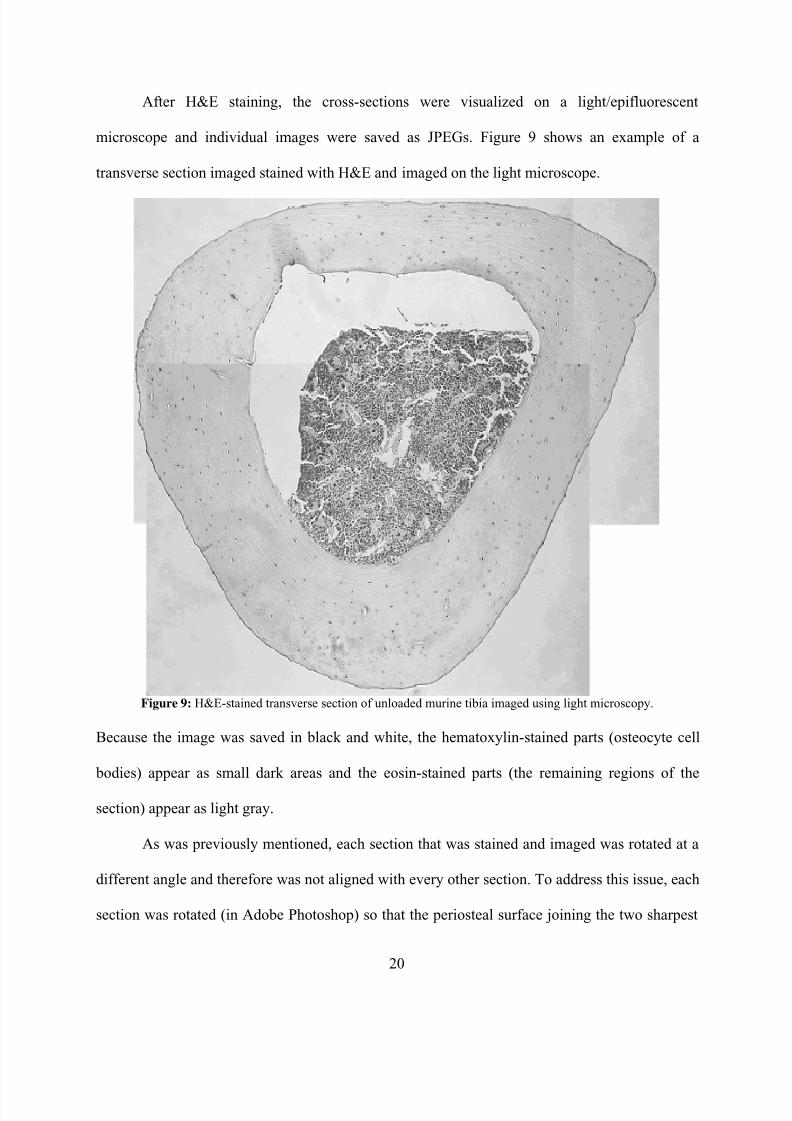
After H&E staining, the cross-sections were visualized on a light/epifluorescent

microscope and individual images were saved as JPEGs. Figure 9 shows an example of a

transverse section imaged stained with H&E and imaged on the light microscope.

Figure 9: H&E-stained transverse section of unloaded murine tibia imaged using light microscopy.

Because the image was saved in black and white, the hematoxylin-stained parts (osteocyte cell

bodies) appear as small dark areas and the eosin-stained parts (the remaining regions of the

section) appear as light gray.

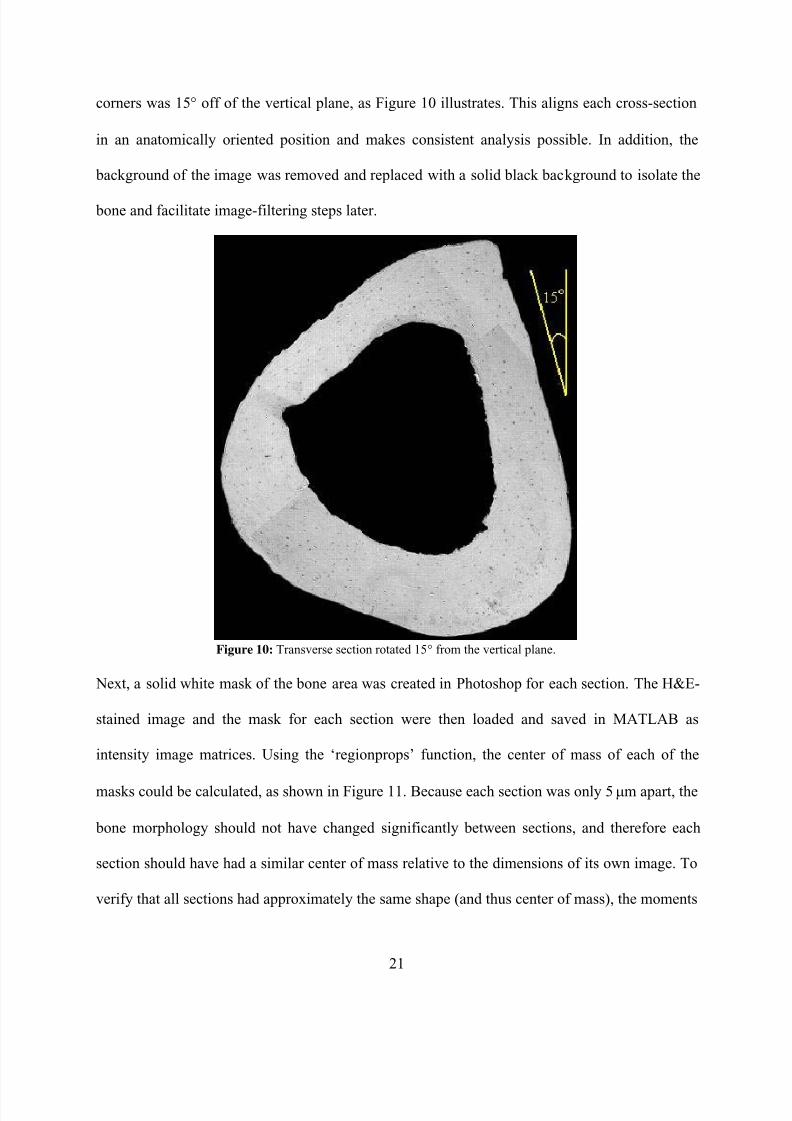
As was previously mentioned, each section that was stained and imaged was rotated at a

different angle and therefore was not aligned with every other section. To address this issue, each

section was rotated (in Adobe Photoshop) so that the periosteal surface joining the two sharpest

20



corners was 15° off of the vertical plane, as Figure 10 illustrates. This aligns each cross-section

in an anatomically oriented position and makes consistent analysis possible. In addition, the

background of the image was removed and replaced with a solid black background to isolate the

bone and facilitate image-filtering steps later.

Figure 10: Transverse section rotated 15° from the vertical plane.

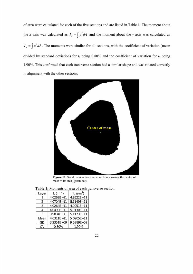
Next, a solid white mask of the bone area was created in Photoshop for each section. The H&E-

stained image and the mask for each section were then loaded and saved in MATLAB as

intensity image matrices. Using the ‘regionprops’ function, the center of mass of each of the

masks could be calculated, as shown in Figure 11. Because each section was only 5 μm apart, the

bone morphology should not have changed significantly between sections, and therefore each

section should have had a similar center of mass relative to the dimensions of its own image. To

verify that all sections had approximately the same shape (and thus center of mass), the moments

21



of area were calculated for each of the five sections and are listed in Table 1. The moment about

the x axis was calculated as and the moment about the y axis was calculated as

. The moments were similar for all sections, with the coefficient of variation (mean

divided by standard deviation) for I x being 0.80% and the coefficient of variation for I y being

1.90%. This confirmed that each transverse section had a similar shape and was rotated correctly

in alignment with the other sections.

∫= dA y I x2

∫= dA x I

y

2

Center of mass

Figure 11: Solid mask of transverse section showing the center of mass of its area (green dot).

Table 1: Moments of area of each transverse section.

Layer Ix (μm4) Iy (μm4)

1 4.0262E+11 4.9522E+11

2 4.0704E+11 5.1149E+11

3 4.0264E+11 4.9051E+11

4 4.0490E+11 5.0130E+11

5 3.9834E+11 5.1173E+11

Mean 4.0311E+11 5.0205E+11

SD 3.2351E+09 9.5289E+09

CV 0.80% 1.90%

22



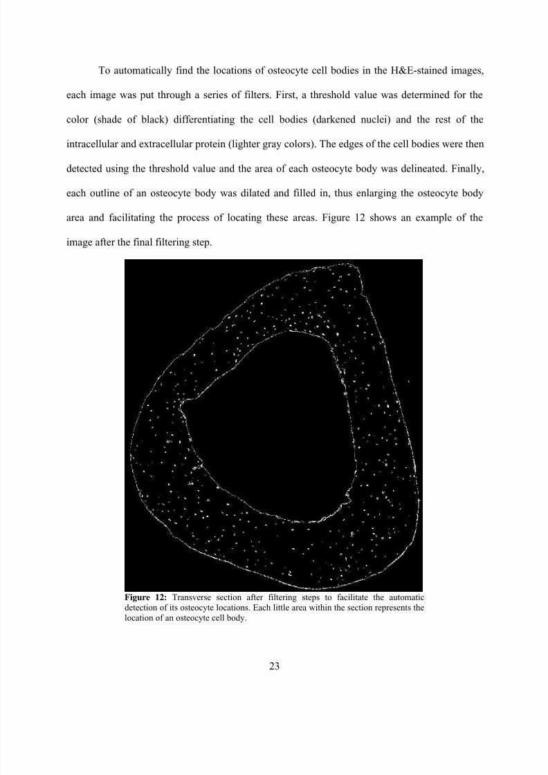
To automatically find the locations of osteocyte cell bodies in the H&E-stained images,

each image was put through a series of filters. First, a threshold value was determined for the

color (shade of black) differentiating the cell bodies (darkened nuclei) and the rest of the

intracellular and extracellular protein (lighter gray colors). The edges of the cell bodies were then

detected using the threshold value and the area of each osteocyte body was delineated. Finally,

each outline of an osteocyte body was dilated and filled in, thus enlarging the osteocyte body

area and facilitating the process of locating these areas. Figure 12 shows an example of the

image after the final filtering step.

Figure 12: Transverse section after filtering steps to facilitate the automaticdetection of its osteocyte locations. Each little area within the section represents thelocation of an osteocyte cell body.

23



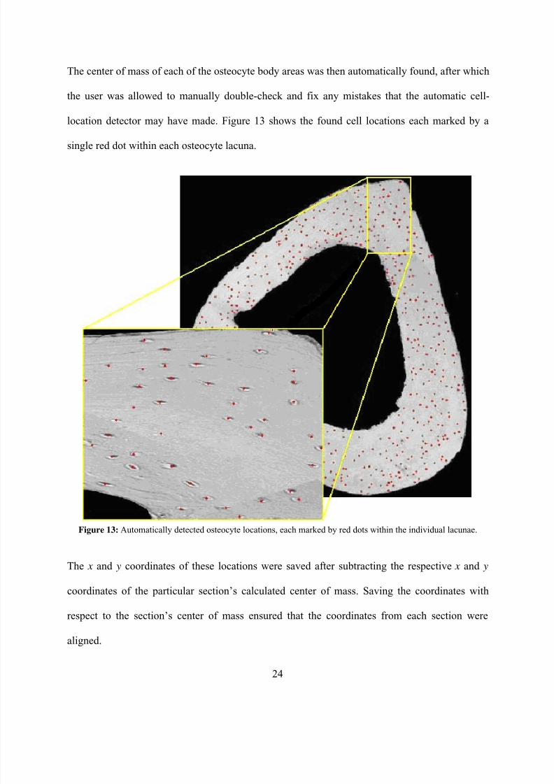
The center of mass of each of the osteocyte body areas was then automatically found, after which

the user was allowed to manually double-check and fix any mistakes that the automatic cell-

location detector may have made. Figure 13 shows the found cell locations each marked by a

single red dot within each osteocyte lacuna.

Figure 13: Automatically detected osteocyte locations, each marked by red dots within the individual lacunae.

The x and y coordinates of these locations were saved after subtracting the respective x and y

coordinates of the particular section’s calculated center of mass. Saving the coordinates with

respect to the section’s center of mass ensured that the coordinates from each section were

aligned.

24



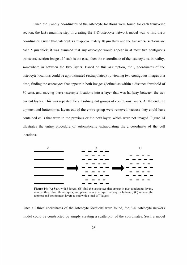
Once the x and y coordinates of the osteocyte locations were found for each transverse

section, the last remaining step in creating the 3-D osteocyte network model was to find the z

coordinates. Given that osteocytes are approximately 10 μm thick and the transverse sections are

each 5 μm thick, it was assumed that any osteocyte would appear in at most two contiguous

transverse section images. If such is the case, then the z coordinate of the osteocyte is, in reality,

somewhere in between the two layers. Based on this assumption, the z coordinates of the

osteocyte locations could be approximated (extrapolated) by viewing two contiguous images at a

time, finding the osteocytes that appear in both images (defined as within a distance threshold of

30 μm), and moving these osteocyte locations into a layer that was halfway between the two

current layers. This was repeated for all subsequent groups of contiguous layers. At the end, the

topmost and bottommost layers out of the entire group were removed because they could have

contained cells that were in the previous or the next layer, which were not imaged. Figure 14

illustrates the entire procedure of automatically extrapolating the z coordinate of the cell

locations.

Figure 14: (A) Start with 5 layers; (B) find the osteocytes that appear in two contiguous layers,remove them from those layers, and place them in a layer halfway in between; (C) remove thetopmost and bottommost layers to end with a total of 7 layers.

Once all three coordinates of the osteocyte locations were found, the 3-D osteocyte network

model could be constructed by simply creating a scatterplot of the coordinates. Such a model

25



provided the basis for morphological analysis to be performed and this data is presented in the

proceeding Results section.

Costs

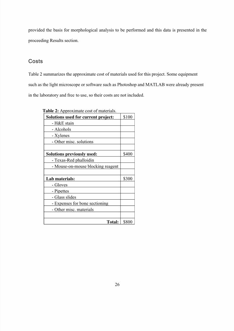
Table 2 summarizes the approximate cost of materials used for this project. Some equipment

such as the light microscope or software such as Photoshop and MATLAB were already present

in the laboratory and free to use, so their costs are not included.

Table 2: Approximate cost of materials.

Solutions used for current project: $100- H&E stain

- Alcohols

- Xylenes

- Other misc. solutions

Solutions previously used: $400

- Texas-Red phalloidin

- Mouse-on-mouse blocking reagent

Lab materials: $300

- Gloves

- Pipettes

- Glass slides

- Expenses for bone sectioning

- Other misc. materials

Total: $800

26



Initial research plan

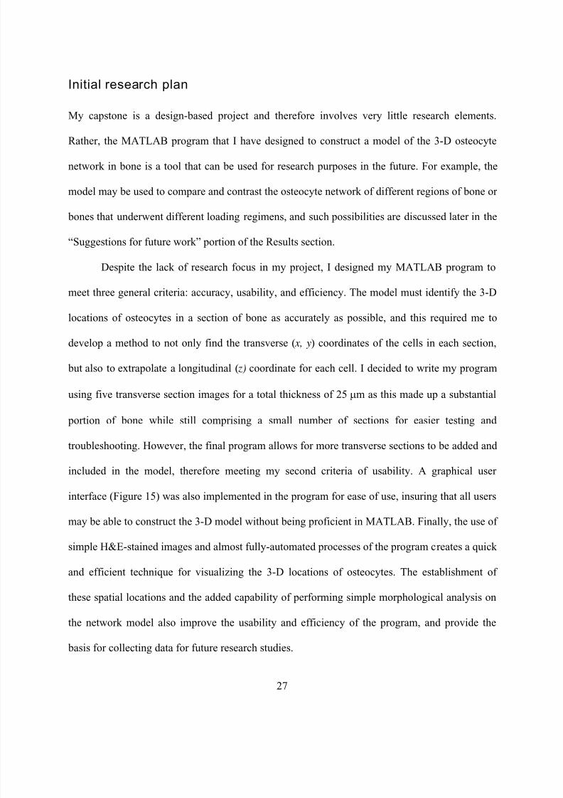
My capstone is a design-based project and therefore involves very little research elements.

Rather, the MATLAB program that I have designed to construct a model of the 3-D osteocyte

network in bone is a tool that can be used for research purposes in the future. For example, the

model may be used to compare and contrast the osteocyte network of different regions of bone or

bones that underwent different loading regimens, and such possibilities are discussed later in the

“Suggestions for future work” portion of the Results section.

Despite the lack of research focus in my project, I designed my MATLAB program to

meet three general criteria: accuracy, usability, and efficiency. The model must identify the 3-D

locations of osteocytes in a section of bone as accurately as possible, and this required me to

develop a method to not only find the transverse ( x, y) coordinates of the cells in each section,

but also to extrapolate a longitudinal ( z) coordinate for each cell. I decided to write my program

using five transverse section images for a total thickness of 25 μm as this made up a substantial

portion of bone while still comprising a small number of sections for easier testing and

troubleshooting. However, the final program allows for more transverse sections to be added and

included in the model, therefore meeting my second criteria of usability. A graphical user

interface (Figure 15) was also implemented in the program for ease of use, insuring that all users

may be able to construct the 3-D model without being proficient in MATLAB. Finally, the use of

simple H&E-stained images and almost fully-automated processes of the program creates a quick

and efficient technique for visualizing the 3-D locations of osteocytes. The establishment of

these spatial locations and the added capability of performing simple morphological analysis on

the network model also improve the usability and efficiency of the program, and provide the

basis for collecting data for future research studies.

27



Figure 15: Graphical user interface for constructing the 3-D osteocyte network model. The user may load the H&E-stained image and solid mask, find and save its osteocyte location coordinates, and pick the contiguous layers toinclude in the network.

28



Results

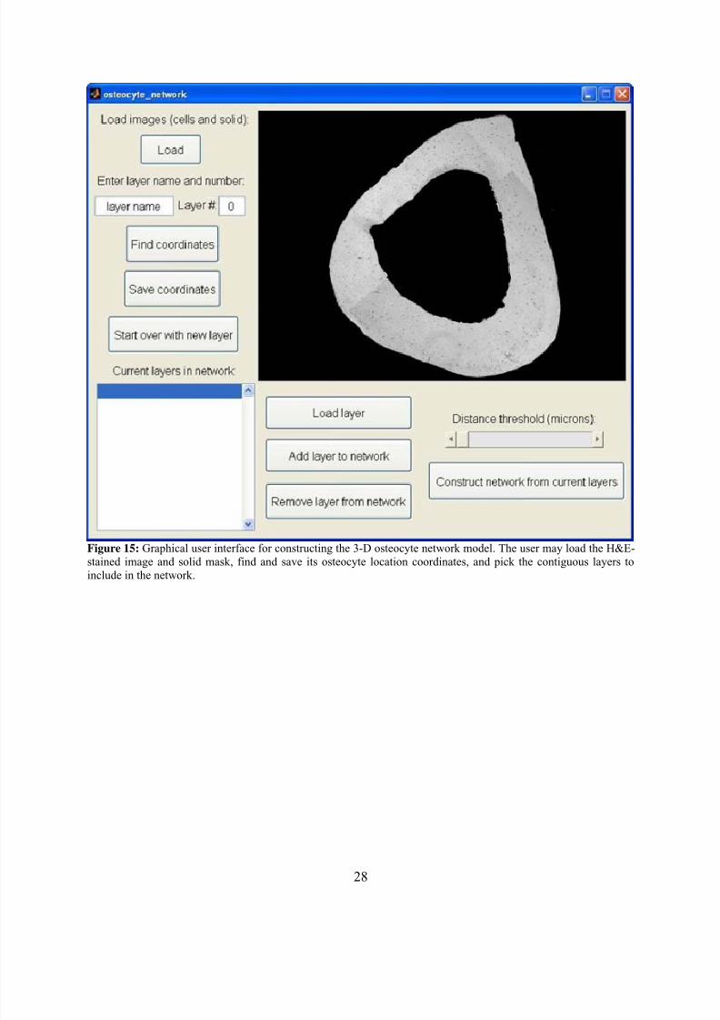
Final timeline

29



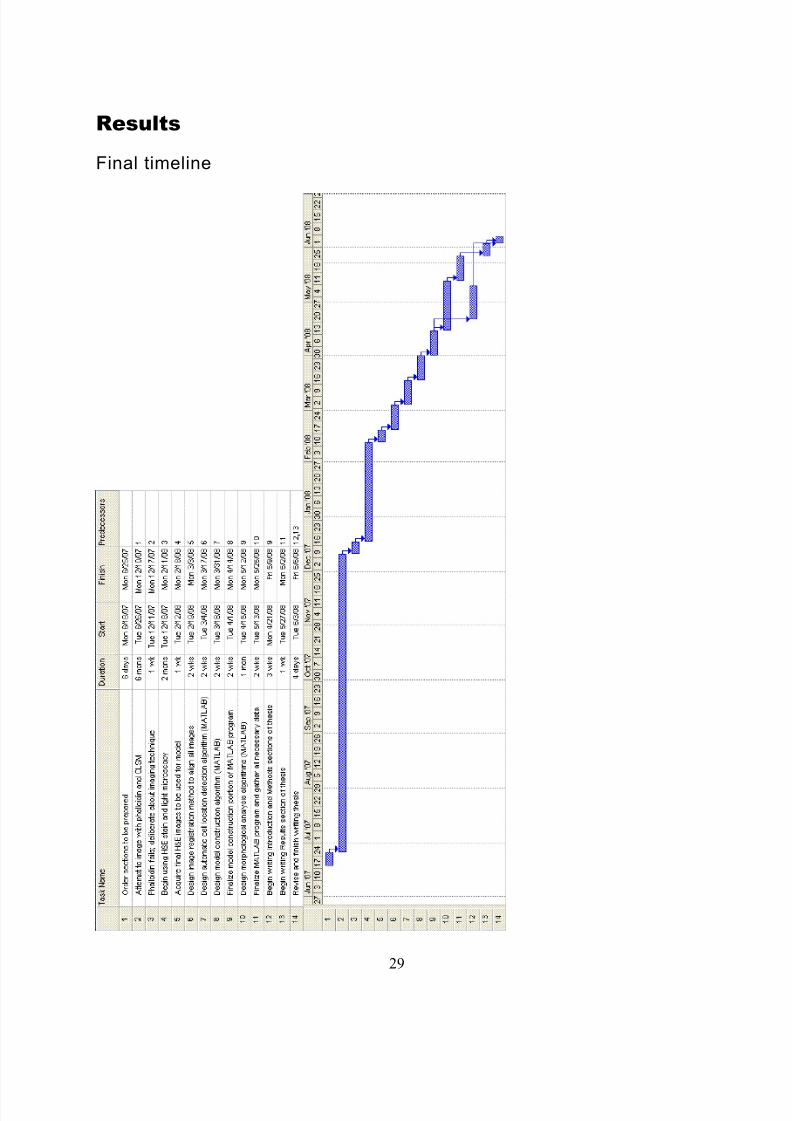
Data

Figure 16 shows the constructed 3-D osteocyte network model with its seven distinctive layers as

described in the Methods section. Each scatterplot point represents the spatial location of an

ostoecyte in the section of bone.

Figure 16: 3-D osteocyte network model showing seven layers constructed from five transverse section images. Theaxes of the model are in micrometers.

30



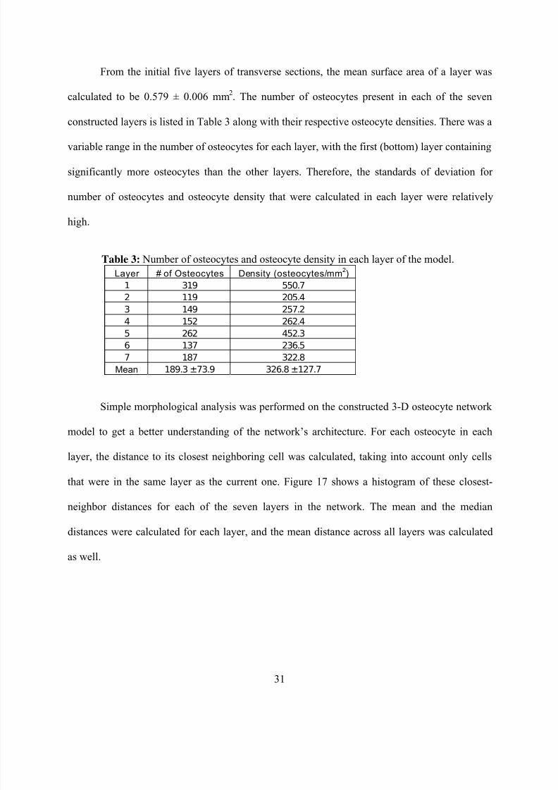
From the initial five layers of transverse sections, the mean surface area of a layer was

calculated to be 0.579 ± 0.006 mm2. The number of osteocytes present in each of the seven

constructed layers is listed in Table 3 along with their respective osteocyte densities. There was a

variable range in the number of osteocytes for each layer, with the first (bottom) layer containing

significantly more osteocytes than the other layers. Therefore, the standards of deviation for

number of osteocytes and osteocyte density that were calculated in each layer were relatively

high.

Table 3: Number of osteocytes and osteocyte density in each layer of the model.

Layer # of Osteocytes Density (osteocytes/mm

2

)1 319 550.7

2 119 205.4

3 149 257.2

4 152 262.4

5 262 452.3

6 137 236.5

7 187 322.8

Mean 189.3 ±73.9 326.8 ±127.7

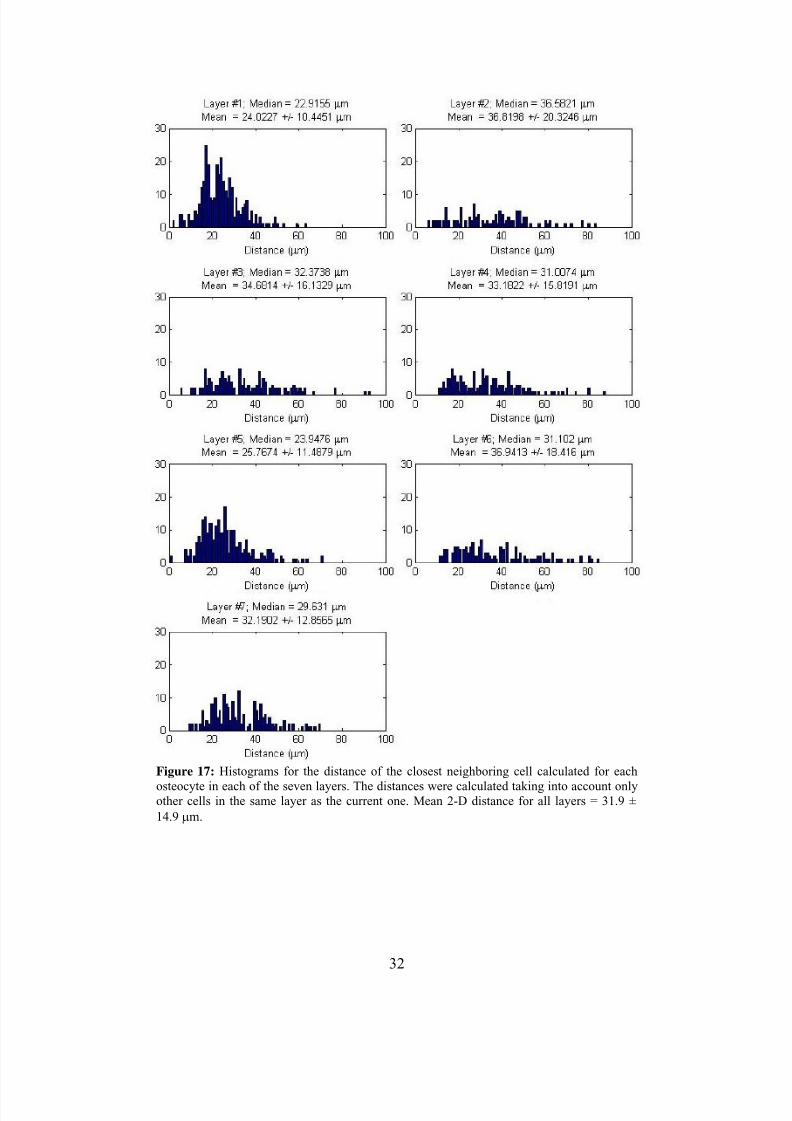
Simple morphological analysis was performed on the constructed 3-D osteocyte network

model to get a better understanding of the network’s architecture. For each osteocyte in each

layer, the distance to its closest neighboring cell was calculated, taking into account only cells

that were in the same layer as the current one. Figure 17 shows a histogram of these closest-

neighbor distances for each of the seven layers in the network. The mean and the median

distances were calculated for each layer, and the mean distance across all layers was calculated

as well.

31



Figure 17: Histograms for the distance of the closest neighboring cell calculated for each

osteocyte in each of the seven layers. The distances were calculated taking into account onlyother cells in the same layer as the current one. Mean 2-D distance for all layers = 31.9 ±

14.9 μm.

32



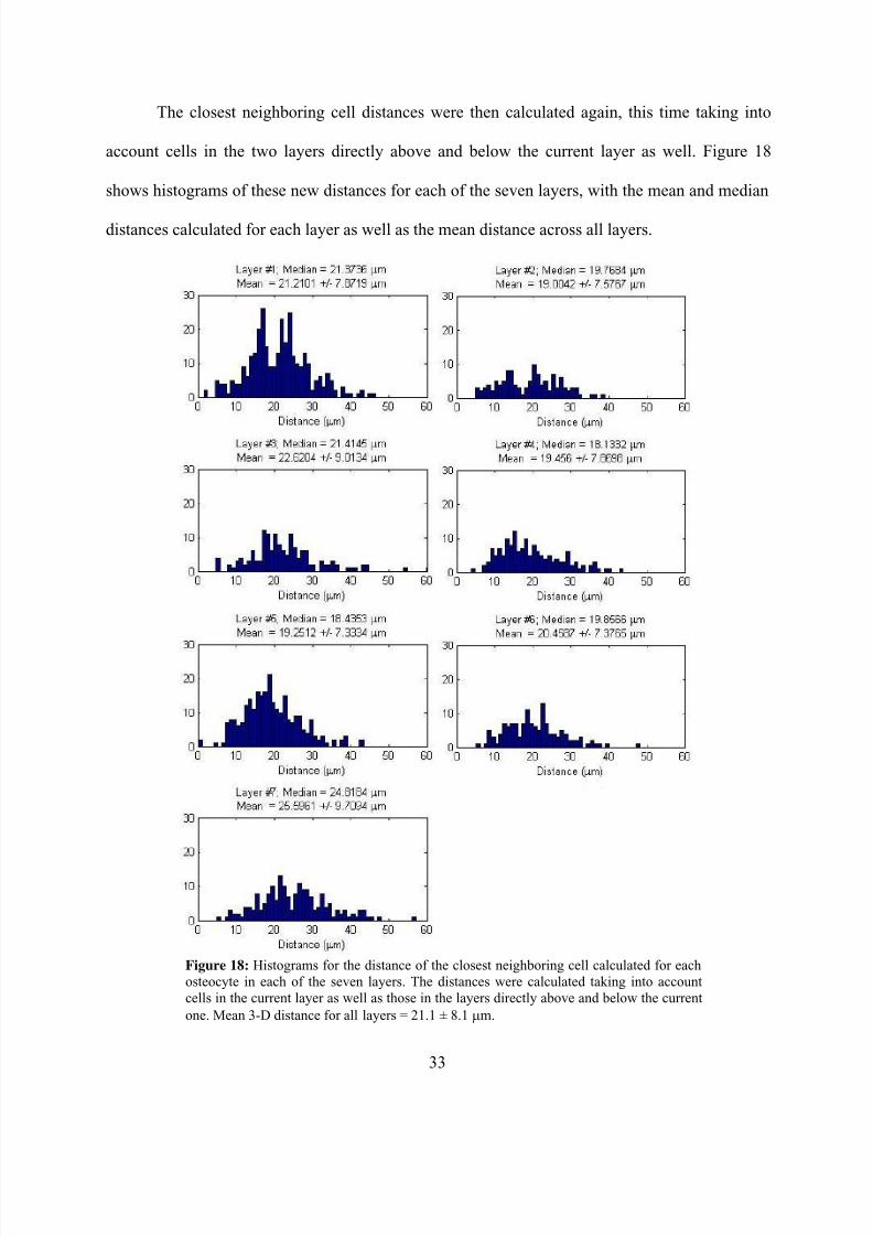
The closest neighboring cell distances were then calculated again, this time taking into

account cells in the two layers directly above and below the current layer as well. Figure 18

shows histograms of these new distances for each of the seven layers, with the mean and median

distances calculated for each layer as well as the mean distance across all layers.

Figure 18: Histograms for the distance of the closest neighboring cell calculated for eachosteocyte in each of the seven layers. The distances were calculated taking into accountcells in the current layer as well as those in the layers directly above and below the current

one. Mean 3-D distance for all layers = 21.1 ± 8.1 μm.

33



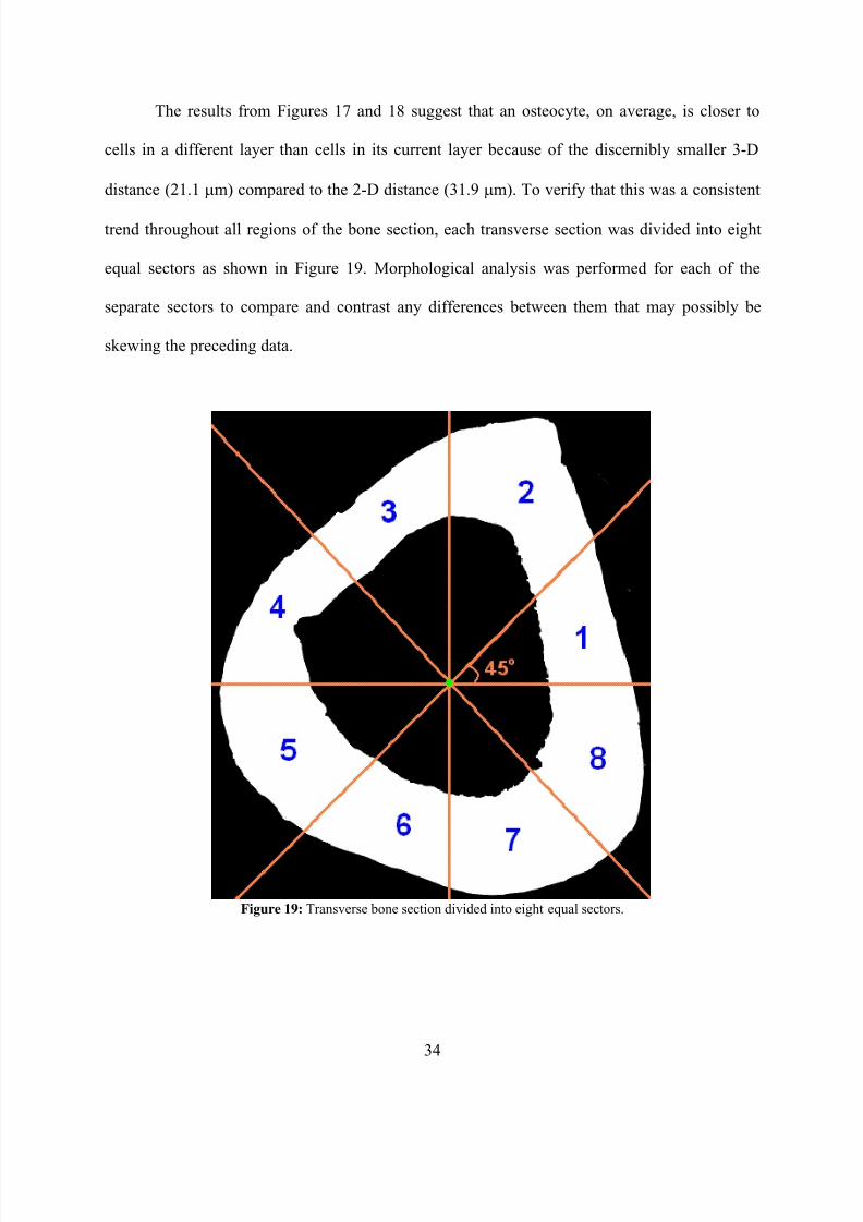
The results from Figures 17 and 18 suggest that an osteocyte, on average, is closer to

cells in a different layer than cells in its current layer because of the discernibly smaller 3-D

distance (21.1 μm) compared to the 2-D distance (31.9 μm). To verify that this was a consistent

trend throughout all regions of the bone section, each transverse section was divided into eight

equal sectors as shown in Figure 19. Morphological analysis was performed for each of the

separate sectors to compare and contrast any differences between them that may possibly be

skewing the preceding data.

Figure 19: Transverse bone section divided into eight equal sectors.

34



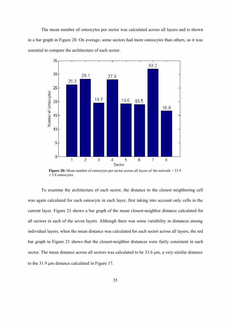
The mean number of osteocytes per sector was calculated across all layers and is shown

in a bar graph in Figure 20. On average, some sectors had more osteocytes than others, so it was

essential to compare the architecture of each sector.

Figure 20: Mean number of osteocytes per sector across all layers of the network = 23.9± 5.8 osteocytes.

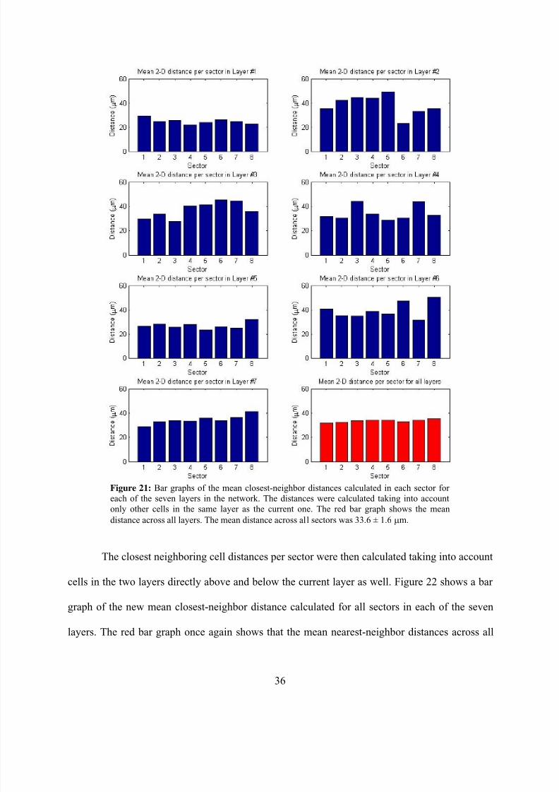
To examine the architecture of each sector, the distance to the closest neighboring cell

was again calculated for each osteocyte in each layer, first taking into account only cells in the

current layer. Figure 21 shows a bar graph of the mean closest-neighbor distance calculated for

all sectors in each of the seven layers. Although there was some variability in distances among

individual layers, when the mean distance was calculated for each sector across all layers, the red

bar graph in Figure 21 shows that the closest-neighbor distances were fairly consistent in each

sector. The mean distance across all sectors was calculated to be 33.6 μm, a very similar distance

to the 31.9 μm distance calculated in Figure 17.

35



Figure 21: Bar graphs of the mean closest-neighbor distances calculated in each sector for each of the seven layers in the network. The distances were calculated taking into accountonly other cells in the same layer as the current one. The red bar graph shows the mean

distance across all layers. The mean distance across all sectors was 33.6 ± 1.6 μm.

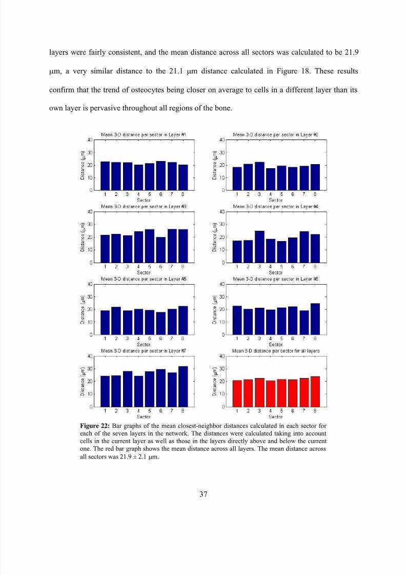
The closest neighboring cell distances per sector were then calculated taking into account

cells in the two layers directly above and below the current layer as well. Figure 22 shows a bar

graph of the new mean closest-neighbor distance calculated for all sectors in each of the seven

layers. The red bar graph once again shows that the mean nearest-neighbor distances across all

36



layers were fairly consistent, and the mean distance across all sectors was calculated to be 21.9

μm, a very similar distance to the 21.1 μm distance calculated in Figure 18. These results

confirm that the trend of osteocytes being closer on average to cells in a different layer than its

own layer is pervasive throughout all regions of the bone.

Figure 22: Bar graphs of the mean closest-neighbor distances calculated in each sector for each of the seven layers in the network. The distances were calculated taking into accountcells in the current layer as well as those in the layers directly above and below the currentone. The red bar graph shows the mean distance across all layers. The mean distance across

all sectors was 21.9 ± 2.1 μm.

37



Experimental/design decisions

As previously mentioned, an experimental decision was made to forego phalloidin staining in

favor of H&E as nearly two quarters worth of testing the phalloidin and confocal laser scanning

microscopy (CLSM) method proved to be unsuccessful. It was determined that an easier and

faster histology protocol would better serve the purposes of the project, and therefore the H&E

protocol was used. If images were obtained from CLSM, then the computer programming

portion of the project would have been less complex since there would no longer be a need to

account for the misalignment of bone transverse sections. However, it was decided that the faster

and simpler method of constructing a 3-D osteocyte network model using H&E-stained images

was worth the tradeoff of having to design an additional technique/algorithm to align the images

before constructing the model.

The method used to make the 3-D osteocyte network model was also simple in design,

therefore improving the usability of the computer program as it only requires users to have a

minimal amount of computer/programming skills and engineering background knowledge. The

concepts of center of mass and moment of area (second moment of inertia) are relatively

straightforward and easily grasped by most users with any basic mathematics background, so

they may use the computer program with a good understanding of how it operates instead of as a

black box.

Despite the simplicity of the program, it has proven to be fairly accurate. Calculating the

moments of area of the transverse sections (Table 1) showed that they were correctly aligned

with little error, and there was also agreement between the morphological data generated by the

model and those in the literature, as will be discussed in the next section. Thus, the decision to

employ simple experimental/design techniques for this project has provided a usable and

efficient method for constructing a 3-D osteocyte network model without sacrificing accuracy.

38



Analysis and conclusions

Overall, my computer program for constructing a 3-D osteocyte network model using H&E-

stained transverse section images performed well and met my three general criteria of efficiency,

usability, and accuracy. The H&E staining protocol only took approximately half the time to

execute as the phalloidin protocol, and the light microscope imaging system was also much more

straightforward to use than the confocal laser scanning microscope. Although using the light

microscope introduced the problem of misalignment between images, the images were re-aligned

in Photoshop and checked in MATLAB by calculating and comparing the moment of area of

each section. As Table 1 shows, the error in alignment (coefficient of variation) was found to be

less than 2%, and thus it was concluded that my manual re-alignment method was acceptably

accurate.

With no user manipulation, the program took less than one minute in total running time to

go from loading the five individual transverse section images to constructing the full 3-D model.

However, as was expected for a simple automated program, there were several errors in the

found osteocyte locations (usually around 50 errors per image). Therefore, to improve the

accuracy of the model, the user had to manually double-check and fix these mistakes that were

made by the automatic cell-locating program, which took up to 10 minutes per image. Although

this method is significantly less laborious than locating every cell by hand, the amount of time it

takes to fix the mistakes generated by the automated program can still be reduced if the image-

filtering algorithm can be improved in the future. This would in turn improve the efficiency and

accuracy of the program and model.

The 3-D osteocyte network shown in Figure 16 has significantly more osteocytes in its

first (bottom) layer compared to its other layers. This discrepancy is unlikely a systematic error

as all layers were put through the same network-construction program to extrapolate the z

39



coordinates of the osteocytes. Therefore, it is likely that there were simply more osteocytes

towards that particular end of the bone, and this could be verified by cutting, imaging, and

analyzing more contiguous transverse sections from that end. Despite the variability in the

number of osteocytes per layer in the network, the average osteocyte density (326.8 ± 127.7

osteocytes/mm2) calculated in Table 3 is within the same range as the density found by other

investigators (an estimated 400-500 osteocytes/mm2 by Power et al. [31]), albeit a little lower.

More transverse sections need to be imaged and analyzed to obtain a better comparison of

osteocyte density, although this preliminary agreement in values between my model’s

calculations and those found in the literature suggests that the imaging and cell-locating

techniques used in this project were fairly accurate.

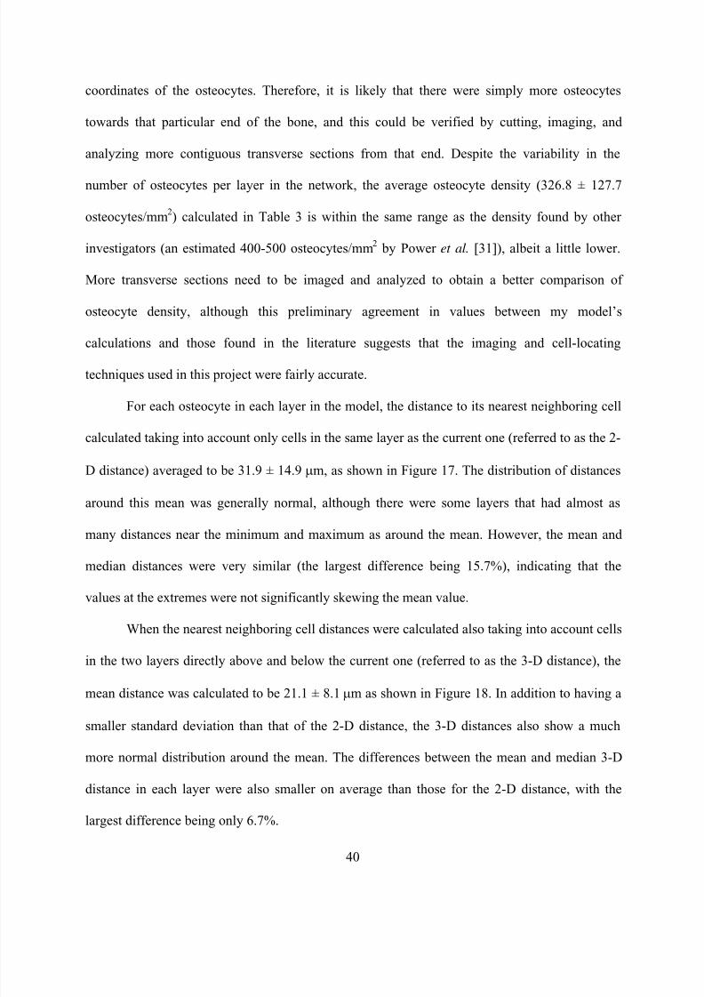
For each osteocyte in each layer in the model, the distance to its nearest neighboring cell

calculated taking into account only cells in the same layer as the current one (referred to as the 2-

D distance) averaged to be 31.9 ± 14.9 μm, as shown in Figure 17. The distribution of distances

around this mean was generally normal, although there were some layers that had almost as

many distances near the minimum and maximum as around the mean. However, the mean and

median distances were very similar (the largest difference being 15.7%), indicating that the

values at the extremes were not significantly skewing the mean value.

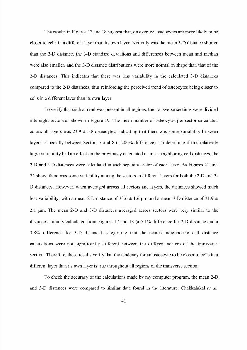
When the nearest neighboring cell distances were calculated also taking into account cells

in the two layers directly above and below the current one (referred to as the 3-D distance), the

mean distance was calculated to be 21.1 ± 8.1 μm as shown in Figure 18. In addition to having a

smaller standard deviation than that of the 2-D distance, the 3-D distances also show a much

more normal distribution around the mean. The differences between the mean and median 3-D

distance in each layer were also smaller on average than those for the 2-D distance, with the

largest difference being only 6.7%.

40



The results in Figures 17 and 18 suggest that, on average, osteocytes are more likely to be

closer to cells in a different layer than its own layer. Not only was the mean 3-D distance shorter

than the 2-D distance, the 3-D standard deviations and differences between mean and median

were also smaller, and the 3-D distance distributions were more normal in shape than that of the

2-D distances. This indicates that there was less variability in the calculated 3-D distances

compared to the 2-D distances, thus reinforcing the perceived trend of osteocytes being closer to

cells in a different layer than its own layer.

To verify that such a trend was present in all regions, the transverse sections were divided

into eight sectors as shown in Figure 19. The mean number of osteocytes per sector calculated

across all layers was 23.9 ± 5.8 osteocytes, indicating that there was some variability between

layers, especially between Sectors 7 and 8 (a 200% difference). To determine if this relatively

large variability had an effect on the previously calculated nearest-neighboring cell distances, the

2-D and 3-D distances were calculated in each separate sector of each layer. As Figures 21 and

22 show, there was some variability among the sectors in different layers for both the 2-D and 3-

D distances. However, when averaged across all sectors and layers, the distances showed much

less variability, with a mean 2-D distance of 33.6 ± 1.6 μm and a mean 3-D distance of 21.9 ±

2.1 μm. The mean 2-D and 3-D distances averaged across sectors were very similar to the

distances initially calculated from Figures 17 and 18 (a 5.1% difference for 2-D distance and a

3.8% difference for 3-D distance), suggesting that the nearest neighboring cell distance

calculations were not significantly different between the different sectors of the transverse

section. Therefore, these results verify that the tendency for an osteocyte to be closer to cells in a

different layer than its own layer is true throughout all regions of the transverse section.

To check the accuracy of the calculations made by my computer program, the mean 2-D

and 3-D distances were compared to similar data found in the literature. Chakkalakal et al.

41



estimated that the length of canaliculi linking adjacent osteocytes in the same transverse plane

was approximately 30 to 40 μm [32], which is in the same range as my program’s calculated

mean 2-D distance of 31.9 ± 13.9 μm. Sugawara et al. were able to use their CLSM-generated

osteocyte network to measure the point-to-point 3-D distance between the centers of mass of

adjacent osteocytes and reported a mean distance of 24.1 ± 2.8 μm [4]. These values are also in

the same range as my program’s calculated nearest neighboring cell 3-D distance of 21.1 ± 8.1

μm. The approximate agreement in morphological data between those previously measured and

those generated by my model not only verifies the accuracy of my program, but also

demonstrates its efficiency. My technique for constructing a 3-D osteocyte network model is

therefore advantageous in that it uses significantly simpler (H&E staining and light microscopy)

and faster (automatic cell detection and model construction) methods than those previously used

to produce equally accurate data.

An interesting result that was obtained from constructing the 3-D osteocyte network

model is that osteocytes are seemingly closer to cells in layers different than their own layer.

Because osteocytes that are closer together are more likely to be connected via their processes

and transmitting signals to each other [33], this result suggests that the longitudinal component

of cell-to-cell communication may have a larger influence on the direction of signaling pathways

than previously recognized. Whether or not osteocytes’ signaling pathways tend to travel in the

longitudinal direction rather than in the transverse direction remains to be validated in future

investigations. The 3-D bone morphology in different parts along the bone’s long axis needs to

be examined to determine the true complex nature of osteocyte signaling pathway directions.

Such analysis may be performed using sections that are cut transversely as well as longitudinally

to verify the accuracy of the z-dimension data. In addition, more detailed imaging methods such

as those employed by Sugawara et al. [4] may be used to determine the exact connections that

42



each osteocyte has to its neighbors in both the transverse and longitudinal directions. These

possible investigations are beyond the scope of this capstone project; however, this project has

demonstrated that obtaining a solid understanding of the direction of signaling pathways requires

the study of bone’s 3-D osteocyte network architecture and specifically the influence of the

longitudinal component of cell-to-cell signaling.

Suggestions for future work

Although my computer program has proven to be quite efficient compared to previously used

methods for analyzing osteocyte networks, improvements may still be made to increase its

efficiency and accuracy. Specifically, if more time was devoted to understanding how to

properly stain the bone with the fluorescent antibody phalloidin, then the images obtained

through CLSM should not only show the spatial location of osteocytes, but also the processes

that connect them. Visualizing exactly how osteocytes are connected is vital to understanding the

direction of their signaling pathways, and is also much more accurate than only knowing the

osteocytes’ spatial locations and inferring their activity based on their distances to each other. In

addition, using phalloidin staining may possibly eliminate the need to cut serial transverse

sections of the bone (and later re-align them) as CLSM is capable of taking serial transverse

images within thick sections of bone. Despite these advantages of phalloidin staining and CLSM,

there is a tradeoff between using complex and expensive techniques to construct a more detailed

model and using faster and simpler techniques to construct a fairly accurate model. Such a

decision must be carefully considered and will depend on the needs of future experiments.

As my capstone project stands now, the technique designed to automatically construct a

3-D osteocyte network model provides the opportunity to analyze the morphology of any given

section of bone in a quick, easy, yet accurate manner. The computer program may be used to

43



construct models of different parts of a section of bone to examine how the osteocyte network

differs in these various sections. Alternatively, models could be constructed for bones that

underwent different loading regimens to compare and contrast how the osteocyte network has

changed in response to the loading. As long as there is a need to quickly examine the

morphology of any type of bone, the computer program may easily be modified according to the

bone’s specifications and then be used for analysis.

The automatically obtained spatial locations of osteocytes may also be incorporated into

the OSL’s ABM to improve the accuracy of its real-time simulations of osteocyte signaling

activity induced by artificially-introduced stimuli. Should it be decided that the ABM’s

simulations in 3-D need to be verified by in vivo experiments, then my computer program may

need to be modified to include the capability of constructing the osteocyte network model using

phalloidin-stained CLSM images that illustrate the physical interconnectivity of osteocytes. The

development of a program that can perform fast and accurate analysis of bone morphology in

addition to being able to show the detailed architecture of the osteocyte network may prove to be

an invaluable tool for investigators to understand mechanotransduction signaling pathways in

bone.

44



Acknowledgements

I would like to thank my advisor, Professor Ted S. Gross, for the opportunity to work at the OSL

and for his time and effort in guiding me through my capstone project. I would also like to thank

the rest of the OSL team, particularly DeWayne Threet for teaching me various immunohisto-

chemistry and imaging techniques and Brandon Ausk for aiding me with MATLAB. Finally, I

would like to acknowledge the additional help with programming that I received from my

classmates Jason Padvorac and Yung-Chun Chen. This capstone project was funded by the

Dean’s Undergraduate Research Award in the University of Washington College of Engineering

and the NIH AR45565.

45



References

1. Rubin, C.T. and L.E. Lanyon, Regulation of bone formation by applied dynamic loads. JBone Joint Surg Am, 1984. 66(3): p. 397-402.

2. Rubin, C.T. and L.E. Lanyon, Regulation of bone mass by mechanical strain magnitude. Calcif Tissue Int, 1985. 37(4): p. 411-7.

3. Gross, T.S., et al., Noninvasive loading of the murine tibia: an in vivo model for the study

of mechanotransduction. J Bone Miner Res, 2002. 17(3): p. 493-501.

4. Sugawara, Y., et al., Three-dimensional reconstruction of chick calvarial osteocytes and

their cell processes using confocal microscopy. Bone, 2005. 36(5): p. 877-83.

5. Srinivasan, S., et al., Low-magnitude mechanical loading becomes osteogenic when rest

is inserted between each load cycle. J Bone Miner Res, 2002. 17(9): p. 1613-20.

6. Riggs, B.L. and L.J. Melton, 3rd, Involutional osteoporosis. N Engl J Med, 1986.314(26): p. 1676-86.

7. Gross, T.S., et al., Why rest stimulates bone formation: a hypothesis based on complex

adaptive phenomenon. Exerc Sport Sci Rev, 2004. 32(1): p. 9-13.

8. Lewiecki, E.M., Prevention and treatment of postmenopausal osteoporosis. ObstetGynecol Clin North Am, 2008. 35(2): p. 301-15.

9. Knothe Tate, M.L. and U. Knothe, An ex vivo model to study transport processes and fluid flow in loaded bone. J Biomech, 2000. 33(2): p. 247-54.

10. Jones, H.H., et al., Humeral hypertrophy in response to exercise. J Bone Joint Surg Am,1977. 59(2): p. 204-8.

11. Rubin, J., C. Rubin, and C.R. Jacobs, Molecular pathways mediating mechanical

signaling in bone. Gene, 2006. 367: p. 1-16.

12. Haapasalo, H., et al., Effect of long-term unilateral activity on bone mineral density of

female junior tennis players. J Bone Miner Res, 1998. 13(2): p. 310-9.

13. American Association of Clinical Endocrinologists medical guidelines for clinical

practice for the prevention and treatment of postmenopausal osteoporosis: 2001 edition,

with selected updates for 2003. Endocr Pract, 2003. 9(6): p. 544-64.

14. Turner, C.H. and F.M. Pavalko, Mechanotransduction and functional response of the

skeleton to physical stress: the mechanisms and mechanics of bone adaptation. J OrthopSci, 1998. 3(6): p. 346-55.

46



15. Knothe Tate, M.L., "Whither flows the fluid in bone?" An osteocyte's perspective. JBiomech, 2003. 36(10): p. 1409-24.

16. Holtrop, M.E. and G.J. King, The ultrastructure of the osteoclast and its functional

implications. Clinical Orthopaedics and Related Research, 1977. 123: p. 177-196.

17. Reilly, G.C., et al., Investigation of the morphology of the lacunocanalicular system of

cortical bone using atomic force microscopy. Ann Biomed Eng, 2001. 29(12): p. 1074-81.

18. Knothe Tate, M.L., et al., The osteocyte. The International Journal of Biochemistry &Cell Biology, 2004. 36: p. 1-8.

19. Stains, J.P. and R. Civitelli, Gap junctions in skeletal development and function. BiochimBiophys Acta, 2005. 1719(1-2): p. 69-81.

20. Bonewald, L.F., Generation and function of osteocyte dendritic processes. JMusculoskelet Neuronal Interact, 2005. 5(4): p. 321-4.

21. Turner, C.H., Three rules for bone adaptation to mechanical stimuli. Bone, 1998. 23(5): p. 399-407.

22. Huiskes, R., If bone is the answer, then what is the question? J. Anat., 2000. 197: p. 145-56.

23. Wolff, J., The Law of Bone Remodeling. 1986, New York: Springer.

24. Kamioka, H., T. Honjo, and T. Takano-Yamamoto, A three-dimensional distribution of

osteocyte processes revealed by the combination of confocal laser scanning microscopy

and differential interference contrast microscopy. Bone, 2001. 28(2): p. 145-9.

25. Krempien, B., et al., The influence of immobilization on osteocyte morphology: osteocyte

differential count and electron microscopical studies. Virchows Arch A Pathol AnatHistol, 1976. 370(1): p. 55-68.

26. Palumbo, C., et al., Osteocyte differentiation in the tibia of newborn rabbit: an

ultrastructural study of the formation of cytoplasmic processes. Acta Anat (Basel), 1990.137(4): p. 350-8.

27. Cooper, J.A., Effects of cytochalasin and phalloidin on actin. J Cell Biol, 1987. 105(4): p.1473-8.

28. Ausk, B.J., T.S. Gross, and S. Srinivasan, An agent based model for real-time signaling

induced in osteocytic networks by mechanical stimuli. J Biomech, 2006. 39(14): p. 2638-46.

47



29. Kamioka, H., et al., Terminal differentiation of osteoblasts to osteocytes is accompanied

by dramatic changes in the distribution of actin-binding proteins. J Bone Miner Res,2004. 19(3): p. 471-8.

30. Brown, H.S. Hematoxylin & Eosin (The Routine Stain). 2002 [cited 2008 May 16];

Available from: http://www.sigmaaldrich.com/img/assets/7361/Primer-H&Emay04.pdf.

31. Power, J., et al., Osteocyte density in aging subjects is enhanced in bone adjacent to

remodeling haversian systems. Bone, 2002. 30(6): p. 859-65.

32. Chakkalakal, D.A., Mechanoelectric transduction in bone. Journal of Materials Research,1989. 4: p. 1034-46.

33. Thi, M.M., et al., Fluid shear stress remodels expression and function of junctional proteins in cultured bone cells. Am J Physiol Cell Physiol, 2003. 284(2): p. C389-403.

Documents

BIOEN 482 Senior Capstone Thesis