Biomedical Image Analytics Using SAS® Viya® · 3 malignant nodules. Benign nodules, on the other hand, have smooth and spherical surfaces more often than not (Niehaus, Raicu, Furst,

1

Paper SAS1961-2018

Biomedical Image Analytics Using SAS® Viya®

Fijoy Vadakkumpadan and Saratendu Sethi, SAS Institute Inc.

ABSTRACT

Biomedical imaging has become the largest driver of health care data growth, generating millions of terabytes of data annually in the US alone. With the release of SAS® ViyaTM 3.3, SAS has, for the first time, extended its powerful analytics environment to the processing and interpretation of biomedical image data. This new extension, available in SAS® Visual Data Mining and Machine Learning, enables customers to load, visualize, process, and save health care image data and associated metadata at scale. In particular, it accommodates both 2-D and 3-D images and recognizes all commonly used medical image formats, including the widely used Digital Imaging and Communications in Medicine (DICOM) standard. The visualization functionality enables users to examine underlying anatomical structures in medical images via exquisite 3-D renderings. The new feature set, when combined with other data analytic capabilities available in SAS Viya, empowers customers to assemble end-to-end solutions to significant, image-based health care problems. This paper demonstrates the new capabilities with an example problem: diagnostic classification of malignant and benign lung nodules that is based on raw computed tomography (CT) images and radiologist annotation of nodule locations.

INTRODUCTION

Biomedical Image processing is an interdisciplinary field that is at the intersection of computer science, machine learning, image processing, medicine, and other fields. The origins of biomedical image processing can be attributed to the accidental discovery of X-rays by Wilhelm Conrad Roentgen in 1895. The discovery made it possible for the first time in the history of humans to noninvasively explore inside the human body before engaging in complex medical procedures. Since then, more methods for medical imaging have been developed, such as computed tomography (CT), magnetic resonance imaging (MRI), ultrasound imaging, single-photon emission computed tomography (SPECT), positron emission tomography (PET), and visible-light imaging. The goal of biomedical image processing is to develop computational and mathematical methods for analyzing such medical images for research and clinical care. The methods of biomedical image processing can be grouped into following broad categories: image segmentation (methods to differentiate between biologically relevant structures such as tissues, organs, and pathologies), image registration (aligning images), and image-based physiological modeling (quantitative assessment of anatomical, physical, and physiological processes).

SAS has a rich history of supporting health and life sciences customers for their clinical data management, analytics, and compliance needs. SAS® Analytics provides an integrated environment for collection, classification, analysis, and interpretation of data to reveal patterns, anomalies, and key variables and relationships, leading ultimately to new insights for guided decision making. Application of SAS® algorithms have enabled patients to transform themselves from being passive recipients to becoming active participants in their own personalized health care. With the release of SAS Viya 3.3, SAS customers can now extend the analytics framework to take advantage of medical images along with statistical, visualization, data mining, text analytics, and optimization techniques for better clinical diagnosis.

Images are supported as a standard SAS data type in SAS Visual Data Mining and Machine Learning, which offers an end-to-end visual environment for machine learning and deep learning—from data access and data wrangling to sophisticated model building and deployment in a scalable distributed framework. It provides a comprehensive suite of programmatic actions to load, visualize, process, and save health care image data and associated metadata at scale in formats such as Digital Imaging and Communication in Medicine (DICOM), Neuroimaging Informatics Technology Initiative (NIFTI), nearly raw raster data (NRRD), and so on. This paper provides a comprehensive overview of the biomedical image processing capabilities in SAS Visual Data Mining and Machine Learning by working through real-world scenarios of building an end-to-end analytic pipeline to classify malignant lung nodules in CT images.

2

END-TO-END BIOMEDICAL IMAGE ANALYTICS IN SAS VIYA

SAS® ViyaTM uses an analytic engine known as SAS® Cloud Analytic Services (CAS) to perform various tasks, including biomedical image analytics. Building end-to-end solutions in SAS Viya typically involves assembling CAS actions, which are the smallest units of data processing that are initiated by a CAS client on a CAS server. CAS actions are packaged into logical groups called action sets. Presently, two action sets, image and bioMedImage, host actions that directly operate on biomedical imagery.

The image action set contains two actions for biomedical image analytics: the loadimages action loads biomedical images from disk into memory, and the saveimages action saves the loaded images from memory to disk. These actions support all common biomedical image formats, including the DICOM standard, which is widely used in clinical settings. The bioMedImage action set currently includes three actions, processBioMedImages, segmentBioMedImages, and buildSurface, for preprocessing, segmentation, and visualization of biomedical images, respectively. At this time, full support is available only for two- and three-dimensional (2-D and 3-D), single-channel biomedical images in these action sets.

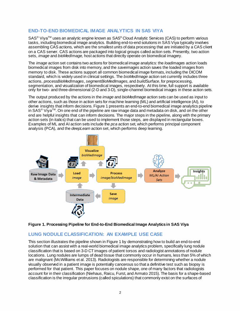
The output produced by the actions in the image and bioMedImage action sets can be used as input to other actions, such as those in action sets for machine learning (ML) and artificial intelligence (AI), to derive insights that inform decisions. Figure 1 presents an end-to-end biomedical image analytics pipeline in SAS® ViyaTM. On one end of the pipeline are raw image data and metadata on disk, and on the other end are helpful insights that can inform decisions. The major steps in the pipeline, along with the primary action sets (in italics) that can be used to implement those steps, are displayed in rectangular boxes. Examples of ML and AI action sets include the pca action set, which performs principal component analysis (PCA), and the deepLearn action set, which performs deep learning.

Figure 1. Processing Pipeline for End-to-End Biomedical Image Analytics in SAS Viya

LUNG NODULE CLASSIFICATION: AN EXAMPLE USE CASE

This section illustrates the pipeline shown in Figure 1 by demonstrating how to build an end-to-end solution that can assist with a real-world biomedical image analytics problem, specifically lung nodule classification that is based on 3-D CT images of patient torsos and radiologist annotations of nodule locations. Lung nodules are lumps of dead tissue that commonly occur in humans, less than 5% of which are malignant (McWilliams et al. 2013). Radiologists are responsible for determining whether a nodule visually observed in a patient image is potentially cancerous so that a definitive test such as biopsy is performed for that patient. This paper focuses on nodule shape, one of many factors that radiologists account for in their classification (Niehaus, Raicu, Furst, and Armato 2015). The basis for a shape-based classification is the irregular protrusions (called spiculations) that commonly exist on the surfaces of

3

malignant nodules. Benign nodules, on the other hand, have smooth and spherical surfaces more often than not (Niehaus, Raicu, Furst, and Armato 2015). This example demonstrates two solutions that can assist with the classification, one based on ML and the other on AI. All client-side source code in this demonstration was written in Python. The SAS Scripting Wrapper for Analytics Transfer (SWAT) package was used to interface with the CAS server, and the Mayavi library (Ramachandran and Varoquaux 2011) was used to perform 3-D visualizations of image-based data.

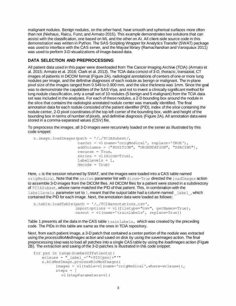
DATA SELECTION AND PREPROCESSING

All patient data used in this paper were downloaded from The Cancer Imaging Archive (TCIA) (Armato et al. 2015; Armato et al. 2016; Clark et al. 2013). The TCIA data consist of 3-D, thoracic, transaxial, CT images of patients in DICOM format (Figure 2A), radiologist annotations of centers of one or more lung nodules per image, and the definitive diagnoses of each nodule as benign or malignant. The in-plane pixel size of the images ranged from 0.549 to 0.900 mm, and the slice thickness was 1mm. Since the goal was to demonstrate the capabilities of the SAS Viya, and not to invent a clinically significant method for lung nodule classification, only a small set of 10 nodules (5 benign and 5 malignant) from the TCIA data set was included in the analyses. For each of these nodules, a 2-D bounding box around the nodule in the slice that contains the radiologist-annotated nodule center was manually identified. The final annotation data for each nodule consisted of the patient identifier (PID), index of the slice containing the nodule center, 2-D pixel coordinates of the top left corner of the bounding box, width and height of the bounding box in terms of number of pixels, and definitive diagnosis (Figure 2A). All annotation data were stored in a comma-separated values (CSV) file.

To preprocess the images, all 3-D images were recursively loaded on the server as illustrated by this code snippet:

s.image.loadImages(path = ’/…/TCIASubset/,

casOut = vl(name='origMedical', replace='TRUE'),

addColumns = {"POSITION", "ORIENTATION", "SPACING"},

recurse = True,

series = vl(dicom=True),

labelLevels = 1,

decode = True)

Here, s is the session returned by SWAT, and the images were loaded into a CAS table named origMedical. Note that the series parameter list with dicom=True directed the loadImages action

to assemble 3-D images from the DICOM files. All DICOM files for a patient were stored in a subdirectory of TCIASubset, whose name matched the PID of that patient. This, in combination with the

labelLevels parameter set to 1, meant that the output table had a column named _label_, which contained the PID for each image. Next, the annotation data were loaded as follows:

s.table.loadTable(path = '/…/TCIAannotations.csv',

importoptions = vl(filetype="csv", getNames=True),

casout = vl(name='trainlabels', replace=True))

Table 1 presents all the data in the CAS table trainlabels, which was created by the preceding code. The PIDs in this table are same as the ones in TCIA repository.

Next, from each patient image, a 3-D patch that contained a center portion of the nodule was extracted using the processBioMedImages action and saved on disk by using the saveImages action. The final preprocessing step was to load all patches into a single CAS table by using the loadImages action (Figure 2B). The extraction and saving of the 3-D patches is illustrated in this code snippet:

for psn in range(numberOfPatients):

wclause = "_label_='"+PID[psn]+"'"

s.bioMedImage.processBioMedImages(

images = vl(table=vl(name='origMedical',where=wclause)),

steps = [

vl(stepParameters=vl(

4

stepType='CROP',

cropParameters=vl(cropType='BASIC',

imageSize=[W[psn],H[psn],2*deltaZ+1],

pixelIndex=[X[psn],Y[psn],Slice[psn]-deltaZ]))),

decode = True,

copyVars = {"_label_","_path_","_type_"},

addColumns={"POSITION", "ORIENTATION", "SPACING"},

casOut = vl(name='noduleRegion', replace=True))

s.image.saveImages(

images = vl(table='noduleRegion', path='_path_'),

subdirectory = 'TrainDataNoduleRegions/',

type = 'nii',

labelLevels = 1)

s.image.loadImages(

casout = vl(name='nodules3D', replace=True),

path = '/…/TrainDataNoduleRegions/',

recurse = True,

addColumns = {"POSITION","ORIENTATION","SPACING"},

labelLevels = 1,

decode = True)

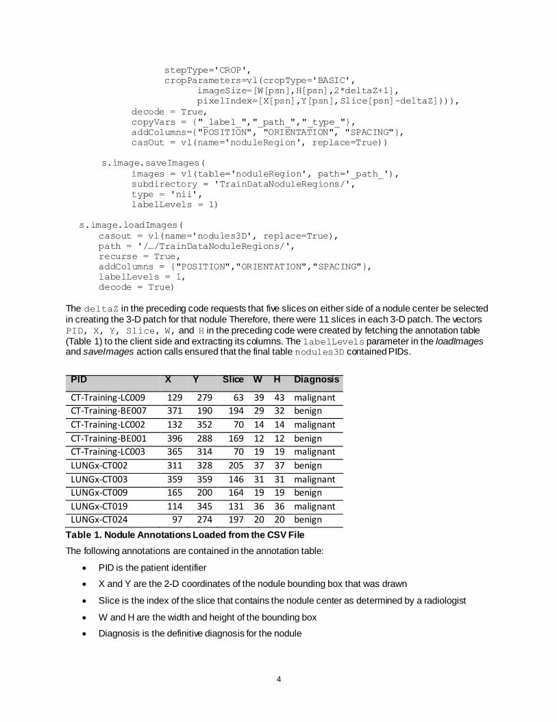
The deltaZ in the preceding code requests that five slices on either side of a nodule center be selected in creating the 3-D patch for that nodule Therefore, there were 11 slices in each 3-D patch. The vectors PID, X, Y, Slice, W, and H in the preceding code were created by fetching the annotation table (Table 1) to the client side and extracting its columns. The labelLevels parameter in the loadImages and saveImages action calls ensured that the final table nodules3D contained PIDs.

PID X Y Slice W H Diagnosis

CT-Training-LC009 129 279 63 39 43 malignant

CT-Training-BE007 371 190 194 29 32 benign


CT-Training-BE001 396 288 169 12 12 benign


LUNGx-CT002 311 328 205 37 37 benign

LUNGx-CT003 359 359 146 31 31 malignant

LUNGx-CT009 165 200 164 19 19 benign

LUNGx-CT019 114 345 131 36 36 malignant

LUNGx-CT024 97 274 197 20 20 benign

Table 1. Nodule Annotations Loaded from the CSV File

The following annotations are contained in the annotation table:

PID is the patient identifier

X and Y are the 2-D coordinates of the nodule bounding box that was drawn

Slice is the index of the slice that contains the nodule center as determined by a radiologist

W and H are the width and height of the bounding box

Diagnosis is the definitive diagnosis for the nodule

5

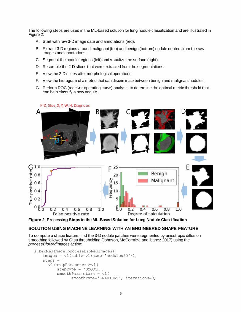
The following steps are used in the ML-based solution for lung nodule classification and are illustrated in Figure 2:

A. Start with raw 3-D image data and annotations (red).

B. Extract 3-D regions around malignant (top) and benign (bottom) nodule centers from the raw images and annotations.

C. Segment the nodule regions (left) and visualize the surface (right).

D. Resample the 2-D slices that were extracted from the segmentations.

E. View the 2-D slices after morphological operations.

F. View the histogram of a metric that can discriminate between benign and malignant nodules.

G. Perform ROC (receiver operating curve) analysis to determine the optimal metric threshold that can help classify a new nodule.

Figure 2. Processing Steps in the ML-Based Solution for Lung Nodule Classification

SOLUTION USING MACHINE LEARNING WITH AN ENGINEERED SHAPE FEATURE

To compute a shape feature, first the 3-D nodule patches were segmented by anisotropic diffusion smoothing followed by Otsu thresholding (Johnson, McCormick, and Ibanez 2017) using the processBioMedImages action:


images = vl(table=vl(name='nodules3D')),

steps = [


stepType = 'SMOOTH',

smoothParameters = vl(

smoothType='GRADIENT', iterations=3,

6

timeStep=0.03))),


stepType='THRESHOLD',

thresholdParameters=vl(

thresholdType='OTSU',

regions=2)))],

decode = True,

copyVars = {"_label_", "_path_", "_id_"},

addColumns = {"POSITION", "ORIENTATION", "SPACING"},

casOut = vl(name='masks3D', replace=True))

See Figure 2C for example images after segmentation. Note that multiple processing steps are performed in sequence in a single call to the processBioMedImages action. Smoothed surfaces of the nodule regions were then constructed using the buildSurface action, as follows:

s.biomedimage.buildsurface(

images = vl(table=vl(name='masks3D')),

intensities = {1},

smoothing = vl(iterations=3),

outputVertices = vl(name='noduleVertices',replace=True),

outputFaces = vl(name='noduleFaces',replace=True))

The action produces two output CAS tables, outputVertices and outputFaces, which contain lists of vertices and triangles of the generated surfaces (one surface per nodule). Surfaces and original gray-scale images that correspond to a few sample nodules were then fetched to the client side and visualized together by using the Mayavi method (Figure 2C), to qualitatively assess the segmentation accuracy.

Next, each segmented 3-D nodule image was split into individual 2-D slices in the transaxial direction so that each slice could be analyzed as a separate observation. This conversion was done using the EXPORT_PHOTO feature of the processBioMedImages action as follows:


images = vl(table=vl(name='masks3D')),

steps = [vl(stepParameters=vl(stepType='EXPORT_PHOTO'))],

decode = True,

copyVars={"_label_"},

casOut = vl(name='masks', replace=True))

The resulting images (Figure 2D) in the masks CAS table were in a format that was accepted by the

photographic image processing actions in the image action set. Then, the processImages action was used to resize the 2-D images to have a uniform size of 32×32 and to perform morphological opening (Johnson, McCormick, and Ibanez 2017):

pgm = "length _path_ varchar(*);

_path_=PUT(_bioMedId_*1000+_sliceIndex_, 5.);"

s.image.processImages(

imageTable = vl(

name='masks',

computedVars={"_path_"},

computedVarsProgram=pgm),

casOut = vl(name='masksScaled', replace='TRUE'),

imageFunctions = [

vl(functionOptions=vl(

functionType="RESIZE",

width=32,

height=32)),


functionType="THRESHOLD",

7

type="BINARY",

value=0))],

decode=True)


imageTable = vl(

name='masks',

computedVars={"_path_"},


casOut = vl(name='masksScaled', replace='TRUE'),

imageFunctions = [


functionType="MORPHOLOGY",

method="ERODE",

kernelWidth=3,

KernelHeight=3)),



method="ERODE",

kernelWidth=3,

KernelHeight=3)),



method="DILATE",

kernelWidth=3,

KernelHeight=3)),



method="DILATE",

kernelWidth=3,

KernelHeight=3))],

decode = True)

The preceding code computes a new column, _path_, which is used later to uniquely identify each 2-D

slice. The thresholding step was necessary after resizing because resizing performs interpolation, which made the image nonbinary. The critical operation here, the morphological opening, performed by the second action call eliminated small and thin regions that constituted a significant part of spiculations. As such, the malignant nodule patches “lost” a significant number of foreground pixels, whereas benign ones retained most of their pixels (Figure 2D and 2E). Based on this result, the shape metric was defined as the relative difference in the number of foreground pixels of a nodule patch between the masksScaled and masksFinal tables. In the following, this metric is called the degree of speculation (DOS).

To compute the DOS metric for each nodule patch, the flattenImages action was used to separate the value of each pixel of that nodule in the masksScaled table into individual columns, and the sum of these values was fetched to the client side, as follows:


imageTable = 'masksScaled',

casOut = vl(name='masksScaledColor', replace='TRUE'),

imageFunctions = [


functionType="CONVERT_COLOR",

type="GRAY2COLOR"))],

decode=True)

s.image.flattenImageTable(

imageTable = 'masksScaledColor',

8

casOut = vl(name='masksScaledFlat', replace='TRUE'),

width = 32,

height = 32)

pgm = "nz = c1";

for num in range(2, commonW*commonH*3 + 1):

pgm += "+c"+str(num)

scaledSum = s.fetch(

table = vl(

name='masksScaledFlat',

computedVars={"nz"},


fetchVars={'_path_', '_label_', 'nz'},

to = 1000)['Fetch']

Here, the conversion of the gray-scale images into color was necessary because the flattenImages action assumes that all images have three channels. Next, the same sequence of operations was performed on the masksFinal table to fetch the sums into another table, scaledFinal. Then, the two tables were

joined on the _path_ variable, and the relative difference between the sums in each row was calculated. The histogram of the DOS metric (Figure 2F) shows a bimodal distribution, demonstrating that the metric can discriminate between benign and malignant nodules. A receiver operating characteristic (ROC) analysis revealed an optimal threshold of 0.08 for the metric (Figure 2G). The classification accuracy of the metric was 85% as per a 10-fold cross validation.

SOLUTION USING ARTIFICIAL INTELLIGENCE WITH A CONVOLUTIONAL NEURAL NETWORK

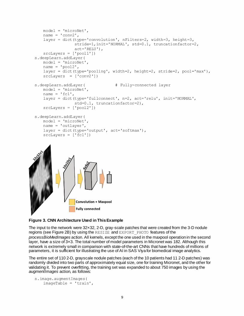
This section uses an alternative solution to assist with lung nodule classification. It uses a convolutional neural network (CNN) to demonstrate the application of artificial intelligence (AI) features that are available in SAS Viya for biomedical image analytics. CNN is a deep learning architecture that has been found to be most effective in image processing. . The following code defines a network, called Micronet, which has just three main layers (Figure 3), including two convolution + maxpool layers, and one fully connected layer:

s.deepLearn.buildModel(

model = vl(name='microNet', replace=True),

type='CNN')

s.deepLearn.addLayer( # Input

model = 'microNet',

name = 'images',

layer = dict(type='input', nchannels=1, width=32, height=32))

s.deepLearn.addLayer( # First convolution+maxpool layer

model = 'microNet',

name = 'conv1',

layer = dict(type='convolution', nFilters=1, width=3, height=3,

stride=1, init='NORMAL', std=0.1, truncationfactor=2,

act='RELU'),

srcLayers = ['images'])

s.deepLearn.addLayer(

model = 'microNet',

name = 'pool1',

layer = dict(type='pooling', width=3, height=3, stride=3, pool='max'),

srcLayers = ['conv1'])

s.deepLearn.addLayer( # Second convolution+maxpool layer

9

model = 'microNet',

name = 'conv2',

layer = dict(type='convolution', nFilters=2, width=3, height=3,

stride=1,init='NORMAL', std=0.1, truncationfactor=2,

act='RELU'),

srcLayers = ['pool1'])


model = 'microNet',

name = 'pool2',

layer = dict(type='pooling', width=2, height=2, stride=2, pool='max'),

srcLayers = ['conv2'])

s.deepLearn.addLayer( # Fully-connected layer

model = 'microNet',

name = 'fc1',

layer = dict(type='fullconnect', n=2, act='relu', init='NORMAL',

std=0.1, truncationfactor=2),

srcLayers = ['pool2'])


model = 'microNet',

name = 'outlayer',

layer = dict(type='output', act='softmax'),

srcLayers = ['fc1'])

Figure 3. CNN Architecture Used in This Example

The input to the network were 32×32, 2-D, gray-scale patches that were created from the 3-D nodule regions (see Figure 2B) by using the RESIZE and EXPORT_PHOTO features of the

processBioMedImages action. All kernels, except the one used in the maxpool operation in the second layer, have a size of 3×3. The total number of model parameters in Micronet was 182. Although this network is extremely small in comparison with state-of-the-art CNNs that have hundreds of millions of parameters, it is sufficient for illustrating the use of AI in SAS Viya for biomedical image analytics.

The entire set of 110 2-D, grayscale nodule patches (each of the 10 patients had 11 2-D patches) was randomly divided into two parts of approximately equal size, one for training Micronet, and the other for validating it. To prevent overfitting, the training set was expanded to about 750 images by using the augmentImages action, as follows:

s.image.augmentImages(

imageTable = 'train',

10

cropList = [{'useWholeImage': True,

'mutations': {

'verticalFlip': True, 'horizontalFlip': True,

'sharpen': True, 'darken': True, 'lighten': True,

'colorJittering': True, 'colorShifting': True,

'rotateRight': True, 'rotateLeft': True,

'pyramidUp': True, 'pyramidDown': True}}],

casOut = vl(name='trainAug', replace=True))

Here, a set of new images was created from each image in the original training via operations such as flipping, rotation, and color changes. The output CAS table trainAug contains the original images along with the newly created ones.

Micronet was then trained asynchronously in 20 epochs as follows:

s.deepLearn.dltrain(

model = 'microNet',

table = 'trainAug',

seed = 99,

input = ['_image_','_label_'],

target = '_label_',

nominal = ['_label_'],

modelweights = vl(name='weights', replace=True),

learningOpts = vl(miniBatchSize=1, maxEpochs=20, learningRate=0.001,

aSyncFreq=1, algorithm='ADAM'))

Note that the _label_ column contained the true diagnosis for each image. The primary output of training is the optimal values of model parameters. These parameters are contained in the CAS table weights, which was then used to score against the validation set as follows:

s.dlscore(model = 'microNet',

initWeights = 'weights',

table = 'test',

copyVars = ['_label_', "_image_"],

layerOut = vl(name='layerOut', replace=True),

casout = vl(name='scored', replace=True))

This scoring resulted in a misclassification error of about 5%. The error varies slightly between different executions of the solution because of the nondeterministic steps involved, including the random splitting of the data into two sets and the stochastic optimization in training.

DISCUSSION

The goals of this paper are to introduce the various SAS Viya components for biomedical image processing and to provide step-by-step illustrations of how to assemble those components to solve real-world biomedical image analytics problems. Two CAS action sets, image and bioMedImage, currently host all actions that directly operate on biomedical imagery. Lung nodule classification is used as an example to illustrate how to assemble these actions in combination with other SAS Viya actions to build pipelines that convert raw biomedical image data and annotations into insights that can help make decisions. Two biomedical image analytic approaches, one using machine learning (ML) and the other using artificial intelligence (AI) are demonstrated.

The choice between ML and AI is application-specific; both approaches have pros and cons. First, the ML solution to the lung nodule classification problem requires the segmentation of gray-scale images in order to separate the foreground (that is, the nodule pixels) from the background. Generally speaking, segmentation is a very challenging task and there is no single algorithm that works across all tissue types. In contrast, the AI solution operates directly on gray-scale images. Secondly, the ML solution provides a continuous metric, the degree of speculation (DOS). Such descriptive metrics are sometimes

11

helpful in clinical medicine, such as to assess progression of disease or response to therapy. The AI solution relies on optimization of CNN parameters that are based on data, and it provides only a binary classification of the images. By and large, it is not feasible to identify the physical meaning of various CNN parameters. Finally, the AI solution has a better classification accuracy than the ML solution, perhaps because the CNN parameters capture multiple shape features from the training data.

It is important to note that the methodologies and results in this paper are for illustrating SAS Viya capabilities; they are not clinically significant. In particular, more systematic studies with larger data sets have reported that shape features have less than 80% accuracy in classifying lung nodules (Niehaus, Raicu, Furst, and Armato 2015). The classification accuracies reported here are overestimated, because the example uses only 10 patients, who were selected from the TCIA data set based on image quality rather than selected randomly. Also, individual 2-D patches were treated as independent observations. In reality, 2-D slices from the same 3-D patch are correlated, and this dependence between slices leads to accuracy overestimation during cross validation.

CONCLUSION

With the recent release of SAS Viya, SAS has, for the first time, extended its platform to directly process and interpret biomedical image data. This new extension, available in SAS Visual Data Mining and Machine Learning, enables customers to load, visualize, process, and save health care image data and associated metadata at scale. Specific examples demonstrate how the new action sets, when combined with other data analytic capabilities available in SAS Viya, such as machine learning and artificial intelligence, empowers customers to assemble end-to-end solutions to significant, image-based health care problems. The complete source code of the examples demonstrated in this paper is publicly available free of cost (SAS Institute Inc. 2018).

Upcoming releases of SAS Viya will build on the foundation that this paper demonstrates. Future development efforts include elimination of the need to save intermediate results back to disk—for example by introducing the capability to process images with image-specific parameters. Also, the bioMedImage action set will be expanded by adding dedicated actions that perform standard segmentation and analysis of biomedical images.

REFERENCES

Armato, S. G., Hadjiiski, L. M., Tourassi, G. D., Drukker, K., Giger, M. L., Li, F., Redmond, G., et al. 2015. “Special Section Guest Editorial: LUNGx Challenge for Computerized Lung Nodule Classification: Reflections and Lessons lLearned.” Journal of Medical Imaging, 020103.

Armato, S. G., Drukker, K., Li, F., Hadjiiski, L., Tourassi, G. D., Kirby, J. S., Clarke, L. P., et al. 2016. “LUNGx Challenge for Computerized Lung Nodule Classification.” Journal of Medical Imaging, 044506.

Clark, K., Vendt, B., Smith, K., Freymann, J., Kirby, J., Koppel, P., Moore, S., et al. 2013. “The Cancer Imaging Archive (TCIA): Maintaining and Operating a Public Information Repository.” Journal of Digital Imaging, 1045–1057.

Johnson, H. J., McCormick, M. M., and Ibanez, L. 2017. The ITK Software Guide: Introduction and Development Guidelines. New York: Kitware, Inc.

McWilliams, A., Tammemagi, M. C., Mayo, J. R., Roberts, H., Liu, G., Soghrati, K., Yasufuku, K., et al. 2013. "Probability of Cancer in Pulmonary Nodules Detected on First Screening CT."New England Journal of Medicine, 910–919.

Niehaus, R., Raicu, D. S., Furst, J., and Armato, S. 2015. “Toward Understanding the Size Dependence of Shape Features for Predicting Spiculation in Lung Nodules for Computer-Aided Diagnosis.” Journal of Digital Imaging, 704–717.

Ramachandran, P., and Varoquaux, G. 2011. “Mayavi: 3D Visualization of Scientific Data” IEEE Computing in Science & Engineering. Computing in Science & Engineering, 40–51.

SAS Institute, Inc. (2018, April 8). SAS® ViyaTM Programming - Biomedical Image Analytics. Retrieved from Github: https://github.com/sassoftware/sas-viya-programming/blob/master/python/biomedical-image-analytics/lung-nodule-classification-sgf2018.ipynb

12

ACKNOWLEDGMENTS

The authors thank the Society of Photographic Instrumentation Engineers (SPIE), American Association of Physicists in Medicine (AAPM), National Cancer Institute (NCI), and TCIA for providing all patient data that are used in this paper. They also thank Anne Baxter her for editorial review.

RECOMMENDED READING

SAS® Visual Data Mining and Machine Learning 8.2: Programming Guide

CONTACT INFORMATION

Your comments and questions are valued and encouraged. Contact the authors at:

Fijoy Vadakkumpadan SAS Institute, Inc. 919 531 1943 [email protected]

Saratendu Sethi SAS Institute, Inc. 919 531 0597 [email protected]

SAS and all other SAS Institute Inc. product or service names are registered trademarks or trademarks of SAS Institute Inc. in the USA and other countries. ® indicates USA registration.

Other brand and product names are trademarks of their respective companies.

mailto:[email protected]

mailto:[email protected]

Documents

Biomedical Image Analytics Using SAS® Viya® · 3 malignant nodules. Benign nodules, on the other hand, have smooth and spherical surfaces more often than not (Niehaus, Raicu, Furst,