Blind detection of equalization errors in communication systems

IEEE TRANSACTIONS ON INFORMATION THEORY, VOL. 43, NO. 2, MARCH 1997 469

Blind Detection of Equalization Errorsin Communication Systems

Kutluyıl Dogancay, Member, IEEE, and Rodney A. Kennedy,Member, IEEE

Abstract—In adaptive channel equalization, transmitted sym-bol estimates at the equalizer output may be in error because ofexcessive channel noise, convergence of the equalizer to a “closed-eye” local minimum, or error propagation if the equalizer hasa decision feedback structure. This paper is concerned with thedetection of equalization errors (i.e., errors in transmitted symbolestimates) in a blindfolded manner whereby no direct access tothe channel input is required. The detection problem is castinto a binary hypothesis testing framework. Assuming a linearcommunication channel that is time-invariant during the test in-terval, a relationship between the presence of equalization errorsand time variations in the underlying linear model taking thetransmitted symbol estimates to the equalizer input is established.Based on this relationship, a uniformly most powerful test isconstructed to detect the presence of equalization errors in finite-length observations. Finite sample size and asymptotic detectionperformance of the test is studied. A method for estimating theequalization delay without direct access to the channel input isdeveloped. The effectiveness of the test is illustrated by way ofcomputer simulations.

Index Terms—Error detection, blind equalizers, hypothesistesting, uniformly most powerful tests, least squares estimation,generalized inverses, equalization delay estimation.

I. INTRODUCTION

T HE purpose of adaptive channel equalization is to miti-gate intersymbol interference (ISI) caused by time disper-

sion in the channel response. Equalization is often performedby an adaptive filter at the channel output. The adaptive filterincorporates, or is followed by, a decision device (usuallya simple quantizer), which makes up for minor mismatchesbetween the ideal channel inverse and the adaptive filter,and also performs the task of symbol estimation by mappingcontinuous-valued filter outputs to discrete symbol values.

The decision device output sequence is said to containequalization errors, if it is not a delayed and possibly phase-shifted version of the channel input sequence. The problem of

Manuscript received April 28, 1995; revised April 22, 1996. This work wassupported in part by the Australian Research Council and the CooperativeResearch Centre for Robust and Adaptive Systems. The material in this paperwas presented in part at the 33rd IEEE Conference on Decision and Control,Florida, December 1994.

K. Dogancay was with the Telecommunications Engineering Group andCooperative Research Centre for Robust and Adaptive Systems, ResearchSchool of Information Sciences and Engineering, the Australian NationalUniversity, Canberra, ACT 0200, Australia. He is now with the Department ofElectrical and Electronic Engineering, The University of Melbourne, Parkville,Victoria 3052, Australia.

R. A. Kennedy is with the Telecommunications Engineering Group andCooperative Research Centre for Robust and Adaptive Systems, ResearchSchool of Information Sciences and Engineering, the Australian NationalUniversity, Canberra, ACT 0200, Australia.

Publisher Item Identifier S 0018-9448(97)00624-X.

testing for the presence of equalization errors is particularlyacute in the case of blind channel equalization for two majorreasons: i) in blind channel equalization, adaptation of theequalizer parameters is carried out in the absence of a trainingsequence (i.e., there is no access to the channel input to makea direct comparison between the channel input and equalizeroutput sequences), and ii) popular stochastic gradient-basedblind equalization algorithms for baud-rate equalizers havemultimodal (nonconvex) cost functions, which render themprone to converging to closed-eye local minima (see e.g., [1],[2]). Although the converged local minimum will eventuallybe escaped because of finite stepsize effects [3], [4], thereis no guarantee that this will happen in a reasonably shorttime. Even in conventional channel equalization in whichtraining data is used to acquire information about the channelcharacteristics at the receiver, there is no straightforwardmeans of detecting equalization errors (perhaps caused byexcessive channel noise) once the training session is over.

This paper is concerned with the detection of equaliza-tion errors by utilizing only the information available at theequalizer. The detection problem is cast into a statisticalhypothesis testing framework. A test criterion for the detectionof equalization errors is established based on a relationshipbetween the presence of equalization errors and time variationsin the underlying linear model taking the channel input symbolestimates at the decision device output to the equalizer input.The method of least squares is invoked to implement thiscriterion as a uniformly most powerful statistical test. Nomajor assumptions are made about the channel input signalconstellation, the equalizer structure, or the channel noise.Unlike the convergence test in [5], the test developed in thispaper does not require anya priori knowledge of the channelinput correlation and is not restricted to testing for convergenceto an idealized open-eye parameter setting.

This paper is organized as follows. Section II gives a formaldescription of the detection problem and states the assumptionsmade throughout the paper. Section III develops the testcriterion for the detection of equalization errors. In Section IV,the test criterion is implemented as a statistical hypothesis test.Optimality properties of the resultant test are discussed and theeffects of test parameters on the error detection performanceare studied. Alternative tests based on the same test criterionare also presented. Section V is concerned with choosing thetest parameters in the absence of any knowledge of their exactvalues. A method for estimating the equalization delay withoutdirect access to the channel input is proposed and a practicaltesting procedure is developed. Section VI presents simulation

0018–9448/97$10.00 1997 IEEE

470 IEEE TRANSACTIONS ON INFORMATION THEORY, VOL. 43, NO. 2, MARCH 1997

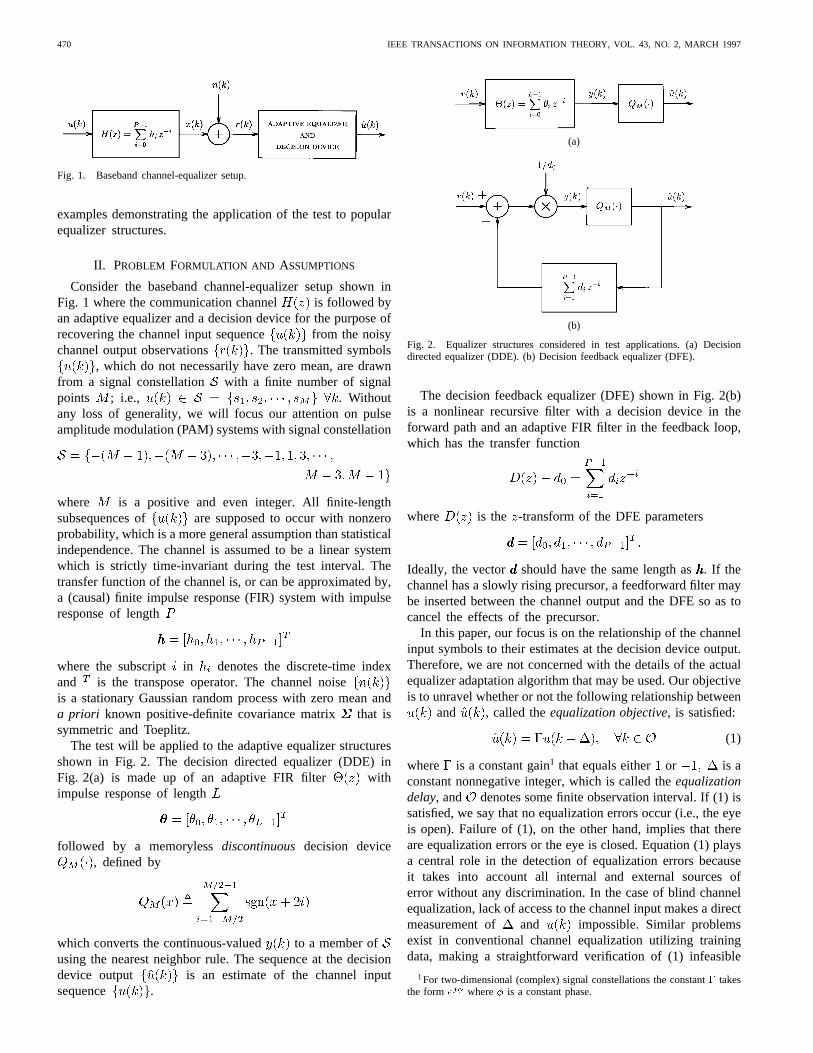
Fig. 1. Baseband channel-equalizer setup.

examples demonstrating the application of the test to popularequalizer structures.

II. PROBLEM FORMULATION AND ASSUMPTIONS

Consider the baseband channel-equalizer setup shown inFig. 1 where the communication channel is followed byan adaptive equalizer and a decision device for the purpose ofrecovering the channel input sequence from the noisychannel output observations . The transmitted symbols

, which do not necessarily have zero mean, are drawnfrom a signal constellation with a finite number of signalpoints ; i.e., . Withoutany loss of generality, we will focus our attention on pulseamplitude modulation (PAM) systems with signal constellation

where is a positive and even integer. All finite-lengthsubsequences of are supposed to occur with nonzeroprobability, which is a more general assumption than statisticalindependence. The channel is assumed to be a linear systemwhich is strictly time-invariant during the test interval. Thetransfer function of the channel is, or can be approximated by,a (causal) finite impulse response (FIR) system with impulseresponse of length

where the subscript in denotes the discrete-time indexand is the transpose operator. The channel noiseis a stationary Gaussian random process with zero mean anda priori known positive-definite covariance matrix that issymmetric and Toeplitz.

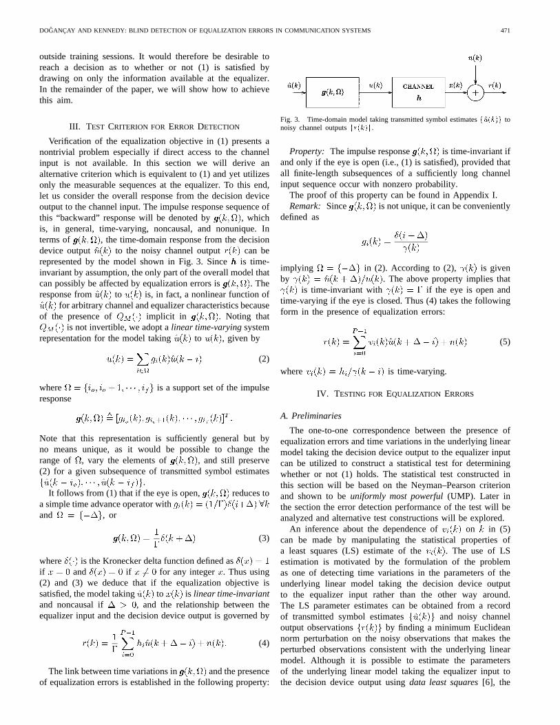
The test will be applied to the adaptive equalizer structuresshown in Fig. 2. The decision directed equalizer (DDE) inFig. 2(a) is made up of an adaptive FIR filter withimpulse response of length

followed by a memorylessdiscontinuousdecision device, defined by

which converts the continuous-valued to a member ofusing the nearest neighbor rule. The sequence at the decisiondevice output is an estimate of the channel inputsequence .

(a)

(b)

Fig. 2. Equalizer structures considered in test applications. (a) Decisiondirected equalizer (DDE). (b) Decision feedback equalizer (DFE).

The decision feedback equalizer (DFE) shown in Fig. 2(b)is a nonlinear recursive filter with a decision device in theforward path and an adaptive FIR filter in the feedback loop,which has the transfer function

where is the -transform of the DFE parameters

Ideally, the vector should have the same length as. If thechannel has a slowly rising precursor, a feedforward filter maybe inserted between the channel output and the DFE so as tocancel the effects of the precursor.

In this paper, our focus is on the relationship of the channelinput symbols to their estimates at the decision device output.Therefore, we are not concerned with the details of the actualequalizer adaptation algorithm that may be used. Our objectiveis to unravel whether or not the following relationship between

and , called theequalization objective, is satisfied:

(1)

where is a constant gain1 that equals either or is aconstant nonnegative integer, which is called theequalizationdelay, and denotes some finite observation interval. If (1) issatisfied, we say that no equalization errors occur (i.e., the eyeis open). Failure of (1), on the other hand, implies that thereare equalization errors or the eye is closed. Equation (1) playsa central role in the detection of equalization errors becauseit takes into account all internal and external sources oferror without any discrimination. In the case of blind channelequalization, lack of access to the channel input makes a directmeasurement of and impossible. Similar problemsexist in conventional channel equalization utilizing trainingdata, making a straightforward verification of (1) infeasible

1For two-dimensional (complex) signal constellations the constant� takesthe formej� where� is a constant phase.

DOGANCAY AND KENNEDY: BLIND DETECTION OF EQUALIZATION ERRORS IN COMMUNICATION SYSTEMS 471

outside training sessions. It would therefore be desirable toreach a decision as to whether or not (1) is satisfied bydrawing on only the information available at the equalizer.In the remainder of the paper, we will show how to achievethis aim.

III. T EST CRITERION FOR ERROR DETECTION

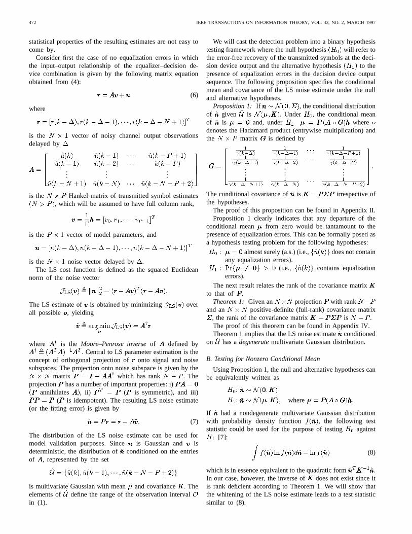
Verification of the equalization objective in (1) presents anontrivial problem especially if direct access to the channelinput is not available. In this section we will derive analternative criterion which is equivalent to (1) and yet utilizesonly the measurable sequences at the equalizer. To this end,let us consider the overall response from the decision deviceoutput to the channel input. The impulse response sequence ofthis “backward” response will be denoted by , whichis, in general, time-varying, noncausal, and nonunique. Interms of , the time-domain response from the decisiondevice output to the noisy channel output can berepresented by the model shown in Fig. 3. Sinceis time-invariant by assumption, the only part of the overall model thatcan possibly be affected by equalization errors is . Theresponse from to is, in fact, a nonlinear function of

for arbitrary channel and equalizer characteristics becauseof the presence of implicit in . Noting that

is not invertible, we adopt alinear time-varyingsystemrepresentation for the model taking to , given by

(2)

where is a support set of the impulseresponse

Note that this representation is sufficiently general but byno means unique, as it would be possible to change therange of , vary the elements of , and still preserve(2) for a given subsequence of transmitted symbol estimates

.It follows from (1) that if the eye is open, reduces to

a simple time advance operator withand , or

(3)

where is the Kronecker delta function defined asif and if for any integer . Thus using(2) and (3) we deduce that if the equalization objective issatisfied, the model taking to is linear time-invariantand noncausal if , and the relationship between theequalizer input and the decision device output is governed by

(4)

The link between time variations in and the presenceof equalization errors is established in the following property:

Fig. 3. Time-domain model taking transmitted symbol estimatesfu(k)g tonoisy channel outputsfr(k)g.

Property: The impulse response is time-invariant ifand only if the eye is open (i.e., (1) is satisfied), provided thatall finite-length subsequences of a sufficiently long channelinput sequence occur with nonzero probability.

The proof of this property can be found in Appendix I.Remark: Since is not unique, it can be conveniently

defined as

implying in (2). According to (2), is givenby . The above property implies that

is time-invariant with if the eye is open andtime-varying if the eye is closed. Thus (4) takes the followingform in the presence of equalization errors:

(5)

where is time-varying.

IV. TESTING FOR EQUALIZATION ERRORS

A. Preliminaries

The one-to-one correspondence between the presence ofequalization errors and time variations in the underlying linearmodel taking the decision device output to the equalizer inputcan be utilized to construct a statistical test for determiningwhether or not (1) holds. The statistical test constructed inthis section will be based on the Neyman–Pearson criterionand shown to beuniformly most powerful(UMP). Later inthe section the error detection performance of the test will beanalyzed and alternative test constructions will be explored.

An inference about the dependence of on in (5)can be made by manipulating the statistical properties ofa least squares (LS) estimate of the . The use of LSestimation is motivated by the formulation of the problemas one of detecting time variations in the parameters of theunderlying linear model taking the decision device outputto the equalizer input rather than the other way around.The LS parameter estimates can be obtained from a recordof transmitted symbol estimates and noisy channeloutput observations by finding a minimum Euclideannorm perturbation on the noisy observations that makes theperturbed observations consistent with the underlying linearmodel. Although it is possible to estimate the parametersof the underlying linear model taking the equalizer input tothe decision device output usingdata least squares[6], the


statistical properties of the resulting estimates are not easy tocome by.

Consider first the case of no equalization errors in whichthe input–output relationship of the equalizer–decision de-vice combination is given by the following matrix equationobtained from (4):

(6)

where

is the vector of noisy channel output observationsdelayed by

......

...

is the Hankel matrix of transmitted symbol estimates, which will be assumed to have full column rank,

is the vector of model parameters, and

is the noise vector delayed by .The LS cost function is defined as the squared Euclidean

norm of the noise vector

The LS estimate of is obtained by minimizing overall possible , yielding

where is the Moore–Penrose inverseof defined by. Central to LS parameter estimation is the

concept of orthogonal projection of onto signal and noisesubspaces. The projection onto noise subspace is given by the

matrix which has rank . Theprojection has a number of important properties: i)

annihilates , ii) ( is symmetric), and iii)( is idempotent). The resulting LS noise estimate

(or the fitting error) is given by

(7)

The distribution of the LS noise estimate can be used formodel validation purposes. Since is Gaussian and isdeterministic, the distribution of conditioned on the entriesof , represented by the set

is multivariate Gaussian with meanand covariance . Theelements of define the range of the observation intervalin (1).

We will cast the detection problem into a binary hypothesistesting framework where the null hypothesis will refer tothe error-free recovery of the transmitted symbols at the deci-sion device output and the alternative hypothesis to thepresence of equalization errors in the decision device outputsequence. The following proposition specifies the conditionalmean and covariance of the LS noise estimate under the nulland alternative hypotheses.

Proposition 1: If , the conditional distributionof given is . Under , the conditional meanof is and, under wheredenotes the Hadamard product (entrywise multiplication) andthe matrix is defined by

......

...

The conditional covariance of is irrespective ofthe hypotheses.

The proof of this proposition can be found in Appendix II.Proposition 1 clearly indicates that any departure of the

conditional mean from zero would be tantamount to thepresence of equalization errors. This can be formally posed asa hypothesis testing problem for the following hypotheses:

almost surely (a.s.) (i.e., does not containany equalization errors).

(i.e., contains equalizationerrors).

The next result relates the rank of the covariance matrixto that of .

Theorem 1: Given an projection with rankand an positive-definite (full-rank) covariance matrix

, the rank of the covariance matrix is .The proof of this theorem can be found in Appendix IV.Theorem 1 implies that the LS noise estimateconditioned

on has adegeneratemultivariate Gaussian distribution.

B. Testing for Nonzero Conditional Mean

Using Proposition 1, the null and alternative hypotheses canbe equivalently written as

where

If had a nondegenerate multivariate Gaussian distributionwith probability density function , the following teststatistic could be used for the purpose of testing against

[7]:

(8)

which is in essence equivalent to the quadratic form .In our case, however, the inverse of does not exist since itis rank deficient according to Theorem 1. We will show thatthe whitening of the LS noise estimate leads to a test statisticsimilar to (8).


Let be a singular value decompositionwhere is an unitary matrix and

is an diagonal matrix of the singular values with. Consider the following

whitening transformation for the LS noise estimate:

(9)

where

diag

The transformed vector has conditional covariance

(10)

According to (9) and (10), can be partitioned as

(11)

where the vector has a white Gaussiandistribution conditioned on with unit variance.

Theorem 2: The vector in (11) has nonzero conditionalmean if and only if the conditional mean of is nonzero.

The proof of this theorem is given in Appendix V.Recognizing that is the Moore–Penrose

inverse of [8], we will consider the following test statisticas an alternative to (8) for noninvertible:

(12a)

(12b)

(12c)

where (12c) follows from (12b) using the relationand the definition of . According to Proposition 1 andTheorem 2, under , the entries of all have zero meanswith unit variance, implying that has acentral chi-squaredistribution with degrees of freedom. Under ,however, has a nonzero mean and thereforeis distributedaccording to thenoncentralchi-square distribution withdegrees of freedom and noncentrality parameter

which is strictly positive if by Theorem 2. The detectionproblem described at the beginning of this subsection can nowbe reduced to a one-sided test of thesimple null hypothesis

versus thecompositealternative hypothesis.

Definition 1 (Uniformly Most Powerful Tests):A test ofversus is uniformly most powerful (UMP) with

significance level if its probability of false alarm is equal toand its power (probability of detection) is uniformly greater

than the power of any other test whose significance level isless than or equal to .

Definition 2 (Monotone-Likelihood Ratio ):The real-para-meter family of densities parametrized by is saidto havemonotone-likelihood ratioif the real-valued function(likelihood ratio)

is a nondecreasing function of for any .Theorem 3 (UMP One-Sided Tests):Let be a real-valued

random variable whose density function is parametrized by.If has a monotone-likelihood ratio, then the threshold test

is the UMP test with significance level for testingversus .

The proof of this theorem is given in [9].The noncentral chi-square distribution has monotone-

likelihood ratio [9], [10]. Therefore, by Theorem 3, thethreshold test

(13)

is the UMP test of versus . The testthreshold is determined by where is theprobability of false alarm

(14)

The power (probability of detection) of the test is given by

(15)

In (14) and (15), , denotes the condi-tional probability density function of under the respectivehypotheses .

C. Relationship of the Noncentrality Parameterto the Test Power

A central chi-square random variable with degrees offreedom, where , can be approximated by a Gaussianrandom variable using the following square-root transforma-tion, also known as Fisher’s result [11, pp. 399–401]:

which is equivalent to

(16)


Using (16) and assuming that , the significancelevel of the test can be written in terms of the test threshold

as follows:

where denotes themodified complementary errorfunction, which is related to the more familiar error function

through . Thus anapproximate expression for the test thresholdcan be written

(17)

To obtain an approximate closed-form expression for thetest power we will use the following approximation fornoncentral chi-square random variables [12]:

When applied to under , this transformation leads to theexpression

(18)

Substituting (17) in (18) and noting that and, we get the expression at the bottom of

this page. If is fixed, is a monotone increasing functionof

(19)

which will be called the equivalent “signal-to-noise ratio(SNR)” [12]. It is easy to see that increases monotonicallywith if is constant.

Channel Noise Effects:The channel noise showsup in the test statistic through the covariance matrix. Letus assume that has the form where and

is a constant symmetric positive semidefinite matrix. Thenoncentrality parameter is then given by .For a fixed , any decrease in, which is tantamount to anincreased channel output SNR, implies an increase in both

and , resulting in a higher . Therefore, the higher thechannel output SNR, the higher the test power will be.

D. Relationship of Equalization Errorsto the Noncentrality Parameter

To complete our analysis of the detection performance, wewill now consider the contribution of equalization errors to thenoncentrality parameter of the test statistic. Recalling thatisdefined in terms of , we will first investigate the contributionof a single equalization error to the conditional mean.

Theorem 4: If in error, its contribution tois

(20)

where is the error

and is defined as

(21)

with

If or , then .The proof of this theorem can be found in Appendix VI.The overall contribution of equalization errors tois given

by the summation of individual contributions, i.e.,

The condition for an equalization error at time to lead toan increase in and therefore an improvement in the detectionperformance is

(22)

To gain more insight into the above condition we expand theinequality on the right-hand side of (22) using (20)

(23)

Intuitively, the detection performance should improve with anincreasing number of equalization errors. However,cannotbe guaranteed to increase with every equalization error unless(23) is satisfied. The quadratic form on the left-hand sideof (23) is always positive. However, the sign of the right-hand side of (23) is not readily predictable. Therefore, therelationship of equalization errors toremains inconclusive.A proportional increase in with the number of equalization


errors is of lesser importance, albeit still desirable, if someequalization errors result in comparatively large increases in

.

E. Asymptotic Detection Analysis

In this subsection we will derive the necessary conditionsfor the test to be consistent. Although we are primarilyconcerned with the detection of equalization errors in finite-length observations as implied by (1), we will find it usefulto gain insight into the dependence of the test performanceon the sample size . Our first result is concernedwith the asymptotic approximation of the LS noise estimatecovariance .

Theorem 5: If the channel is an FIR system of lengthis second-order stationary, the Gram matrix

has full rank, and has a finite span of dependence,the covariance matrix converges a.s. to as tends toinfinity.

Refer to Appendix VII for the proof of this theorem.The conditional mean expression (37) derived in Appendix

II can be expanded as

Noting that is the channel input counterpart ofdelayedby , it is easy to see that if and are stationaryand ergodic, converges a.s. to and

to as , where

and

Thus can be asymptotically written as

a.s. (24)

It is interesting to note that is determined not only bythe difference between and , but alsosecond-order statistics of the channel input and decision deviceoutput sequences. In (24), the product of the inverse ofthe autocorrelation matrix of and the crosscorrelationmatrix between and produces the estimatesof

The asymptotic conditional mean is given by the differencebetween the noise-free channel output vector

and its estimate

The test is consistent if . Recalling that isa monotone increasing function of, the consistency requires

or, using (19),

where the second limit lies in the finite interval. We assume that the significance level of the

test obeys the inequality . The test is thereforeconsistent if

which implies that the noncentrality parametermust beproportional to , for a finite . Thus theerror detection performance improves with increasingif

is approximately proportional to .

F. Testing for Time-Varying Conditional Mean

The alternative tests presented here are based on the premisethat any change in the conditional mean of the LS noiseestimate from one observation interval to another is a directconsequence of equalization errors. Although two LS noiseestimates obtained from different observations can have thesame nonzero conditional mean, that is extremely unlikelyto happen, barring pathological cases, and will therefore beignored.

Test Statistic Using Two Successive LS Noise Estimates:Letus assume that two LS noise estimatesand are availablefrom successive channel output and decision device outputobservations. The LS noise estimates , willhave multivariate Gaussian distributions with conditional mean

and conditional covariancewhere . The matrices and are definedin exactly the same way as and , except that they areconstructed from successive sets of decision device outputobservations. We wish to test the following hypotheses:

a.s.

The difference between successive LS noise estimatesis distributed according to where

andConsider the quadratic form which has a central chi-

square distribution with degrees of freedom under and anoncentral chi-square distribution withdegrees of freedomand noncentrality parameterunder , whereand [8, Theorem 9.2.3]. Then,the threshold test

(25)

is the UMP test with significance level fortesting the simple hypothesis against the compositehypothesis .

Test Statistic Using a Single Record:We can alternativelytest the hypothesis that two subvectors of have equalconditional means, which would be automatically satisfied ifthe eye were open. The resulting test is similar to (25), butit does not require the computation of from successiveobservations. Let the LS noise estimate be partitioned as


with conditional mean andconditional covariance

Suppose is even so that and each haveentries. Since has a conditional Gaussian distribution (seeProposition 1), will have multivariate Gaussiandistribution with conditional mean and conditionalcovariance . The threshold test

(26)

rejects the null hypothesis with probability of falsealarm , whereand . Equation (26) is a UMP test because thetest statistic has a noncentral chi-square distribution.

V. CHOOSING THE TEST PARAMETERS

We have thus far assumed that the test parametersandare knowna priori. This section considers the implications

of relaxing this assumption by allowing deviations in the testparameters from their true values. Specifically, it will be shownthat a knowledge of some bounds onand is sufficient forthe test in (13) to be applicable. This feature makes the test“robust” with respect to the choice of its parameters.

A. Effects of the Test Parameters on theTest Statistic Distribution

In order to ascertain the consequences of replacingandwith arbitrary numbers and , respectively, we will

consider the following version of (6):

where

is the vector of noisy channel output observationsdelayed by ,

......

...

is the full-rank Hankel matrix of transmitted symbolestimates, the matrix at the bottom of this page is thematrix

shifted in time by is the parameter vectorto be estimated, and is the noise vector delayed by . Incontrast to the case where and are known exactly, the“channel” noise now takes the form andits LS estimate is given by

(27)

where is the projection onto noise subspace.Proposition 2: If , the LS noise estimate

conditioned on the entries of and , represented by the set

is distributed according to where underand irrespective of the hypotheses. We have

under if the following holds:

i)ii) .

The proof of this proposition can be found in Appendix III.If the inequalities of Proposition 2 are not satisfied, the

conditional mean of the LS noise estimate cannot be guar-anteed to be zero under because will not necessarilylie in the column space of . Inequality i) in Proposition 2ensures that the equalization delay is not underestimated, whileinequality ii) requires that be long enough to accommodatethe parameter vector augmented by leading zeros.

In the light of Proposition 2, we maintain that the quadraticform parametrized by

(28)

has a central chi-square distribution with degrees offreedom so long as the eye is open and the inequalities ofProposition 2 are satisfied. If the eye is closed, however,will in general have a noncentral chi-square distribution with

degrees of freedom and noncentrality parameter

(29)

B. Blind Estimation of the Equalization Delay

A blind method for estimating the equalization delay basedon the properties of the crosscorrelation between and

was proposed in [5]. In this subsection, we introducean alternative scheme which exploits the nonzero conditionalmean of when the inequality is violated under

(see Proposition 2). We will assume that inequality ii)of Proposition 2 is always satisfied. A requirement for thedelay estimator to produce the true equalization delayisthat the channel be causal with . If has leading zeros,

......

...


the estimator produces an underestimate ofas the delayintroduced by the leading zeros cannot be detected withoutdirect access to the channel input.

According to Proposition 2, under we have the followingrelationship between in (28) and :

which leads to the following delay estimation procedure:

i) Start with a sufficiently large chosen on physicalgrounds.

ii) Perform the test

(30)

where is defined in (28) and is obtained fromfor a prescribed value of .

iii) If is decided, decrease by one and go back to stepii). If is decided, the delay estimate is .

Since varying affects only in (28), the computation offor different is not expensive once is computed.

C. Testing Procedure

If and satisfy the inequalities of Proposition 2, thecontribution of a single equalization error at time

, to can be written as (cf. (20))

(31)

where is the same as in (21) except that it has size. Given the Hankel structure of , (31) reveals that

equalization errors in the following set will go undetected asthey do not make any contribution to:

(32)

Suppose that and satisfy the inequalities of Propo-sition 2. If the test in (30) results in a decision in favor of

, the following procedure should be applied to unravel anyequalization errors that might have been ignored by the test:

i) Introduce systematic errors in by replacingwith another member of for . Computefor every . An estimate of the equalization delayis given by where is the smallest

for which . While this method forestimating the equalization delay is computationallymore expensive than the one in Section V-B, it has theessential feature of insensitivity to equalization errorsthat belong to the undetectable setin (32).

ii) Likewise, replace with othermembers of and compute the resulting forevery . The channel length estimate is given by

where is the smallest forwhich .

iii) Repeat the test in (30) after substitutingand forand , respectively. The new test statistic may havedifferent parameters.

The above procedure usually needs to be carried out only onceat the first occurrence of a decision on. Steps i) and ii) areessentially aimed at estimating the true test parameters fromtheir initial values obeying the inequalities of Proposition 2.

VI. SIMULATION EXAMPLES

The first simulation example demonstrates the application ofthe test in (30) to the detection of equalization errors resultingfrom ill-convergence in a blind equalization setting. Estimationof the equalization delay when convergence to an open-eyeparameter setting is achieved is also illustrated. The secondexample is concerned with the detection of equalization errorsarising from error propagation in a DFE.

The extent of ISI will be quantified by the so-calledclosed-eye measure(CLEM) defined by

CLEM

where CLEM if the eye is open, and CLEM if theeye is closed.

A. Detection of Equalization Errors Due to Ill-Convergence

Consider the nonminimum-phase FIR channel

which is driven by -ary PAM inputs (i.e., ). Thechannel input sequence is generated by a Markov chainwith state vectorand state transition probability matrix

where the th entry is given by. The initial states are assumed to be equiprobable. The

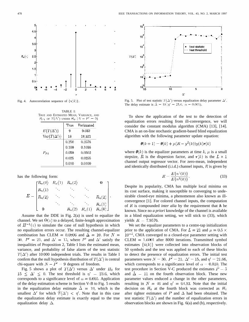
mean of the input sequence is . Notethat need not have zero mean in order for the test in(30) to be applicable. The autocorrelation sequence ofis shown in Fig. 4.

The channel noise is supposed to be a stationarycolored Gaussian process with autocorrelation

, andfor . Thus the covariance matrix of


Fig. 4. Autocorrelation sequence offu(k)g.

TABLE I:TRUE AND ESTIMATED MEAN, VARIANCE, AND

PFA OF T (�0) UNDER H0 (N � P 0 = 9)

has the following form:

......

......

......

......

...

Assume that the DDE in Fig. 2(a) is used to equalize thechannel. We set to a delayed, finite-length approximationof to simulate the case of null hypothesis in whichno equalization errors occur. The resulting channel-equalizercombination has CLEM and . For

and , where and satisfy theinequalities of Proposition 2, Table I lists the estimated mean,variance, and probability of false alarm of the test statistic

after 10 000 independent trials. The results in Table Iconfirm that the null hypothesis distribution of is centralchi-square with degrees of freedom.

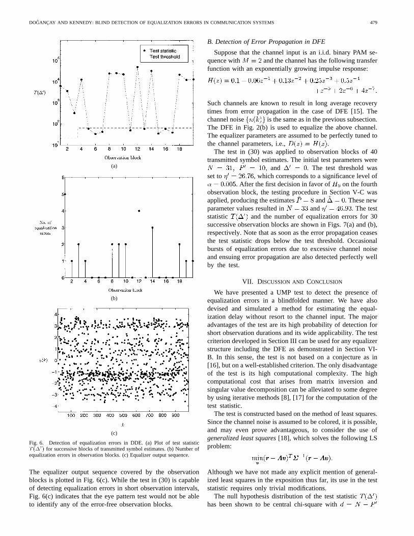
Fig. 5 shows a plot of versus under for. The test threshold is , which

corresponds to a significance level of . Applicationof the delay estimation scheme in Section V-B to Fig. 5 resultsin the equalization delay estimate , which is thesmallest for which . Note that in this casethe equalization delay estimate is exactly equal to the trueequalization delay .

Fig. 5. Plot of test statisticT (�0) versus equalization delay parameter�0.The delay estimate is� = 10 (�0 = 23:6; � = 0:005).

To show the application of the test to the detection ofequalization errors resulting from ill-convergence, we willconsider the constant modulus algorithm (CMA) [13], [14].CMA is an on-line stochastic gradient-based blind equalizationalgorithm with the following parameter update equation:

where is the equalizer parameters at time, is a smallstepsize, is the dispersion factor, and is thechannel output regressor vector. For zero-mean, independentand identically distributed (i.i.d.) channel inputs,is given by

(33)

Despite its popularity, CMA has multiple local minima onits cost surface, making it susceptible to converging to unde-sirable closed-eye minima, a phenomenon also known as ill-convergence [1]. For colored channel inputs, the computationof is compoundedinter alia by the requirement that beknown. Since noa priori knowledge of the channel is availablein a blind equalization setting, we will stick to (33), whichyields .

We set the equalizer parameters to a centre-tap initializationprior to the application of CMA. For and

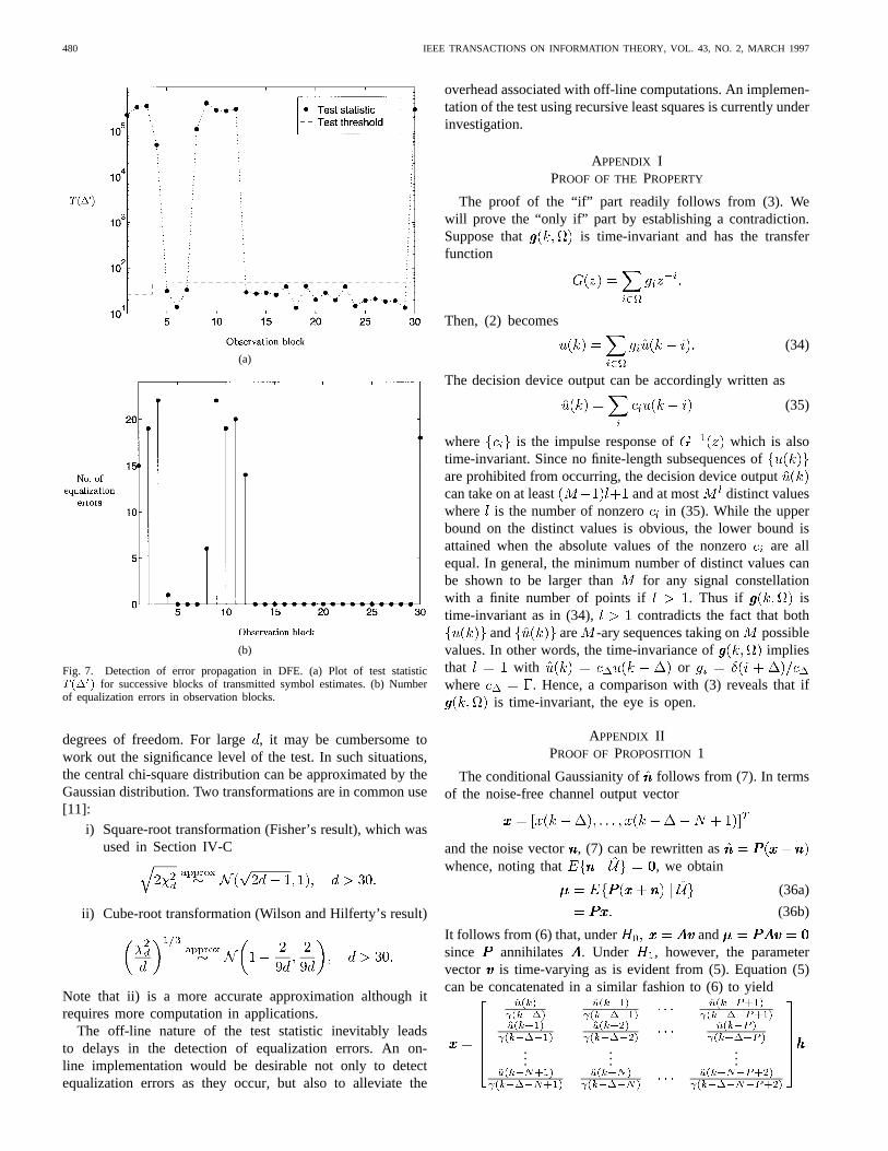
, CMA converged to a closed-eye parameter setting withCLEM after 8000 iterations. Transmitted symbolestimates were collected into observation blocks of50 symbols and the test was applied to each of these blocksto detect the presence of equalization errors. The initial testparameters were andwhich corresponds to a significance level of . Thetest procedure in Section V-C produced the estimatesand on the fourth observation block. These newparameter values enduced a change in the other parameters,resulting in and . Note that the initialdecision on at the fourth block was corrected asafter tighter estimates of and had been obtained. Thetest statistic and the number of equalization errors inobservation blocks are shown in Fig. 6(a) and (b), respectively.


(a)

(b)

(c)

Fig. 6. Detection of equalization errors in DDE. (a) Plot of test statisticT (�0) for successive blocks of transmitted symbol estimates. (b) Number ofequalization errors in observation blocks. (c) Equalizer output sequence.

The equalizer output sequence covered by the observationblocks is plotted in Fig. 6(c). While the test in (30) is capableof detecting equalization errors in short observation intervals,Fig. 6(c) indicates that the eye pattern test would not be ableto identify any of the error-free observation blocks.

B. Detection of Error Propagation in DFE

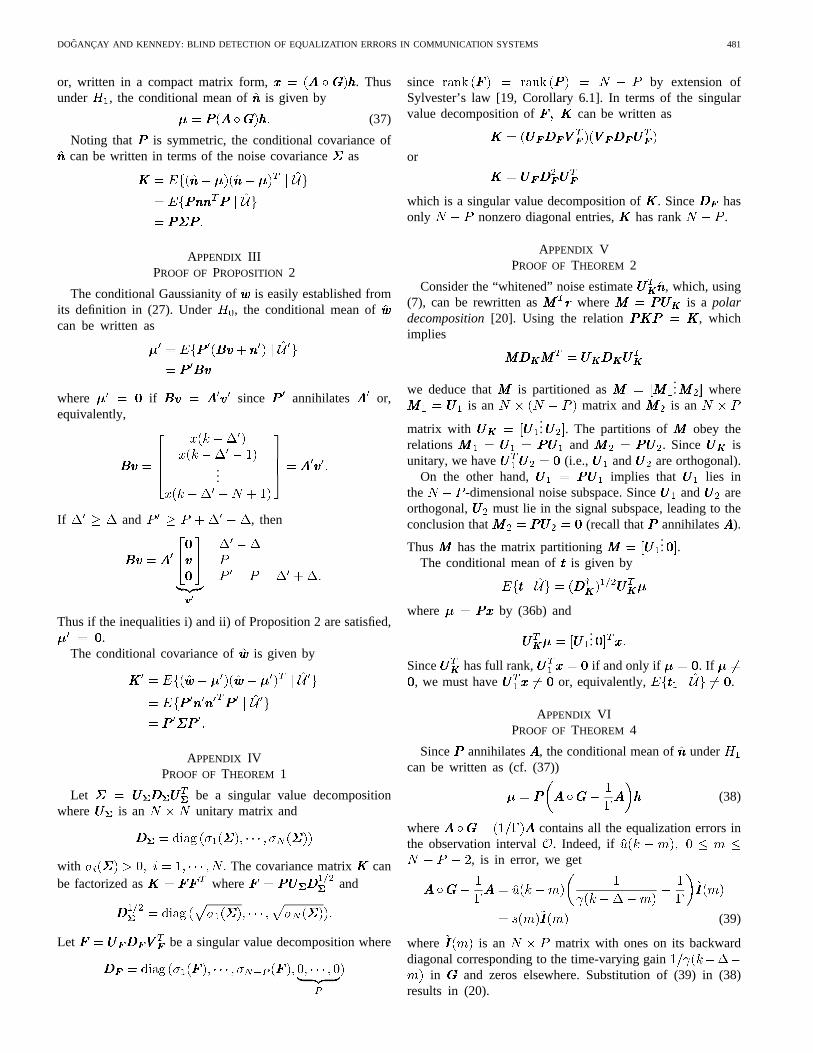
Suppose that the channel input is an i.i.d. binary PAM se-quence with and the channel has the following transferfunction with an exponentially growing impulse response:

Such channels are known to result in long average recoverytimes from error propagation in the case of DFE [15]. Thechannel noise is the same as in the previous subsection.The DFE in Fig. 2(b) is used to equalize the above channel.The equalizer parameters are assumed to be perfectly tuned tothe channel parameters, i.e., .

The test in (30) was applied to observation blocks of 40transmitted symbol estimates. The initial test parameters were

and . The test threshold wasset to , which corresponds to a significance level of

. After the first decision in favor of on the fourthobservation block, the testing procedure in Section V-C wasapplied, producing the estimates and . These newparameter values resulted in and . The teststatistic and the number of equalization errors for 30successive observation blocks are shown in Figs. 7(a) and (b),respectively. Note that as soon as the error propagation ceasesthe test statistic drops below the test threshold. Occasionalbursts of equalization errors due to excessive channel noiseand ensuing error propagation are also detected perfectly wellby the test.

VII. D ISCUSSION AND CONCLUSION

We have presented a UMP test to detect the presence ofequalization errors in a blindfolded manner. We have alsodevised and simulated a method for estimating the equal-ization delay without resort to the channel input. The majoradvantages of the test are its high probability of detection forshort observation durations and its wide applicability. The testcriterion developed in Section III can be used for any equalizerstructure including the DFE as demonstrated in Section VI-B. In this sense, the test is not based on a conjecture as in[16], but on a well-established criterion. The only disadvantageof the test is its high computational complexity. The highcomputational cost that arises from matrix inversion andsingular value decomposition can be alleviated to some degreeby using iterative methods [8], [17] for the computation of thetest statistic.

The test is constructed based on the method of least squares.Since the channel noise is assumed to be colored, it is possible,and may even prove advantageous, to consider the use ofgeneralized least squares[18], which solves the following LSproblem:

Although we have not made any explicit mention of general-ized least squares in the exposition thus far, its use in the teststatistic requires only trivial modifications.

The null hypothesis distribution of the test statistichas been shown to be central chi-square with


(a)

(b)

Fig. 7. Detection of error propagation in DFE. (a) Plot of test statisticT (�0) for successive blocks of transmitted symbol estimates. (b) Numberof equalization errors in observation blocks.

degrees of freedom. For large, it may be cumbersome towork out the significance level of the test. In such situations,the central chi-square distribution can be approximated by theGaussian distribution. Two transformations are in common use[11]:

i) Square-root transformation (Fisher’s result), which wasused in Section IV-C

ii) Cube-root transformation (Wilson and Hilferty’s result)

Note that ii) is a more accurate approximation although itrequires more computation in applications.

The off-line nature of the test statistic inevitably leadsto delays in the detection of equalization errors. An on-line implementation would be desirable not only to detectequalization errors as they occur, but also to alleviate the

overhead associated with off-line computations. An implemen-tation of the test using recursive least squares is currently underinvestigation.

APPENDIX IPROOF OF THE PROPERTY

The proof of the “if” part readily follows from (3). Wewill prove the “only if” part by establishing a contradiction.Suppose that is time-invariant and has the transferfunction

Then, (2) becomes

(34)

The decision device output can be accordingly written as

(35)

where is the impulse response of which is alsotime-invariant. Since no finite-length subsequences ofare prohibited from occurring, the decision device outputcan take on at least and at most distinct valueswhere is the number of nonzero in (35). While the upperbound on the distinct values is obvious, the lower bound isattained when the absolute values of the nonzeroare allequal. In general, the minimum number of distinct values canbe shown to be larger than for any signal constellationwith a finite number of points if . Thus if istime-invariant as in (34), contradicts the fact that both

and are -ary sequences taking on possiblevalues. In other words, the time-invariance of impliesthat with orwhere . Hence, a comparison with (3) reveals that if

is time-invariant, the eye is open.

APPENDIX IIPROOF OF PROPOSITION 1

The conditional Gaussianity of follows from (7). In termsof the noise-free channel output vector

and the noise vector, (7) can be rewritten aswhence, noting that , we obtain

(36a)

(36b)

It follows from (6) that, under andsince annihilates . Under , however, the parametervector is time-varying as is evident from (5). Equation (5)can be concatenated in a similar fashion to (6) to yield

......

...


or, written in a compact matrix form, . Thusunder , the conditional mean of is given by

(37)

Noting that is symmetric, the conditional covariance ofcan be written in terms of the noise covarianceas

APPENDIX IIIPROOF OF PROPOSITION 2

The conditional Gaussianity of is easily established fromits definition in (27). Under , the conditional mean ofcan be written as

where if since annihilates or,equivalently,

...

If and , then

Thus if the inequalities i) and ii) of Proposition 2 are satisfied,.

The conditional covariance of is given by

APPENDIX IVPROOF OF THEOREM 1

Let be a singular value decompositionwhere is an unitary matrix and

with The covariance matrix canbe factorized as where and

Let be a singular value decomposition where

since by extension ofSylvester’s law [19, Corollary 6.1]. In terms of the singularvalue decomposition of can be written as

or

which is a singular value decomposition of. Since hasonly nonzero diagonal entries, has rank .

APPENDIX VPROOF OF THEOREM 2

Consider the “whitened” noise estimate , which, using(7), can be rewritten as where is a polardecomposition[20]. Using the relation , whichimplies

we deduce that is partitioned as... where

is an matrix and is an

matrix with... . The partitions of obey the

relations and . Since isunitary, we have (i.e., and are orthogonal).

On the other hand, implies that lies inthe -dimensional noise subspace. Since and areorthogonal, must lie in the signal subspace, leading to theconclusion that (recall that annihilates ).

Thus has the matrix partitioning... .

The conditional mean of is given by

where by (36b) and

...

Since has full rank, if and only if . If, we must have or, equivalently, .

APPENDIX VIPROOF OF THEOREM 4

Since annihilates , the conditional mean of undercan be written as (cf. (37))

(38)

where contains all the equalization errors inthe observation interval . Indeed, if

, is in error, we get

(39)

where is an matrix with ones on its backwarddiagonal corresponding to the time-varying gain

in and zeros elsewhere. Substitution of (39) in (38)results in (20).


APPENDIX VIIPROOF OF THEOREM 5

The covariance matrix can be written in terms of as

(40)

Since is second-order-stationary, the strong law oflarge numbers (the pointwise-ergodic theorem [21]) implies

a.s.

where

and is a finite matrix. For large , the matrix productcan be approximately written as

(41)

where is the th entry of the covariance matrix ,which is Toeplitz by assumption, and

Under the assumption that has a finite span of depen-dence , we have

a.s.

Similarly, the matrix product can be shown toresult in a finite matrix regardless of . Thus for largecan be approximated by

The above approximation reveals that all the terms of (40)except the first one will vanish as tends to infinity, therebyleading to the conclusion that the LS noise estimate covariance

converges a.s. to the noise covarianceas .

ACKNOWLEDGMENT

The authors would like to thank the anonymous reviewersfor their constructive comments, which have led to consider-able improvement in the exposition of the material.

The authors also wish to acknowledge the funding of theactivities of the Cooperative Research Centre for Robust andAdaptive Systems by the Australian Government under theCooperative Research Centres Program.

REFERENCES

[1] Z. Ding, R. A. Kennedy, B. D. O. Anderson, and C. R. Johnson Jr.,“Ill-convergence of Godard blind equalizers in data communicationsystems,”IEEE Trans. Commun., vol. 39, pp. 1313–1327, Sept. 1991.

[2] C. R. Johnson Jr., “Admissibility in blind adaptive channel equaliza-tion,” IEEE Contr. Syst. Mag., vol. 11, pp. 3–15, Jan. 1991.

[3] J. E. Mazo, “Analysis of decision-directed equalizer convergence,”BellSyst. Tech. J., vol. 59, pp. 1857–1876, Dec. 1980.

[4] O. Macchi and E. Ewada, “Convergence analysis of self-adaptiveequalizers,”IEEE Trans. Inform. Theory, vol. IT-30, pp. 162–176, Mar.1984.

[5] K. Dogancay and R. A. Kennedy, “Testing for the convergence of alinear decision directed equaliser,”IEE Proc. Vision, Image and SignalProcessing, vol. 141, pp. 129–136, Apr. 1994.

[6] R. D. DeGroat and E. M. Dowling, “The data least squares problemand channel equalization,”IEEE Trans. Signal Processing, vol. 41, pp.407–411, Jan. 1993.

[7] J. Segen and A. C. Sanderson, “Detecting change in a time-series,”IEEETrans. Inform. Theory, vol. IT-26, no. 2, pp. 249–255 Mar. 1980.

[8] C. R. Rao and S. K. Mitra,Generalized Inverse of Matrices and ItsApplications. New York, Wiley, 1971.

[9] L. L. Scharf, Statistical Signal Processing: Detection, Estimation, andTime Series Analysis. Reading, MA: Addison-Wesley, 1991.

[10] E. L. Lehmann,Testing Statistical Hypotheses, 2nd ed. New York:Chapman & Hall, 1994.

[11] M. G. Kendall and A. Stuart,The Advanced Theory of Statistics, vol. 1,4th ed. London, U.K.: Charles Griffin, 1977.

[12] M. J. Hinich, “Testing for Gaussianity and linearity of a stationary timeseries,”J. Time Ser. Anal., vol. 3, no. 3, pp. 169–176, 1982.

[13] J. R. Treichler and B. G. Agee, “A new approach to multipath correctionof constant modulus signals,”IEEE Trans. Acoust., Speech, SignalProcessing, vol. ASSP-31, pp. 459–472, Apr. 1983.

[14] D. N. Godard, “Self-recovering equalization and carrier tracking in two-dimensional data communication systems,”IEEE Trans. Commun., vol.COM-28, pp. 1867–1875, Nov. 1980.

[15] R. A. Kennedy and B. D. O. Anderson, “Recovery times of decisionfeedback equalizers on noiseless channels,”IEEE Trans. Commun., vol.COM-36, pp. 1012–1021, Oct. 1987.

[16] R. A. Kennedy, B. D. O. Anderson, and R. R. Bitmead, “Blind adap-tation of decision feedback equalisers: Gross convergence properties,”Int. J. Adaptive Contr. and Sig. Processing, vol. 7, pp. 497–523, 1993.

[17] A. Ben-Israel and D. Cohen, “On iterative computation of generalizedinverses and associated projections,”J. SIAM Numer. Anal., vol. 3, no.3, pp. 410–419, 1966.

[18] G. H. Golub and C. F. Van Loan,Matrix Computations, 2nd ed.Baltimore, MD: Johns Hopkins Univ. Press, 1989.

[19] G. Marsaglia and G. P. H. Styan, “Equalities and inequalities for ranksof matrices,”Linear and Multilinear Algebra, vol. 2, pp. 269–292, 1974.

[20] R. A. Horn and C. R. Johnson,Topics in Matrix Analysis. Cambridge,U.K.: Cambridge Univ. Press, 1991.

[21] R. M. Gray, Probability, Random Processes, and Ergodic Properties.New York: Springer-Verlag, 1988.

Documents

Blind detection of equalization errors in communication systems