Embed Size (px)
Citation preview
Blind Source Separation
based on
Joint Diagonalization of Matrices
with Applications in
Biomedical Signal Processing
Dissertation
zur Erlangung des akademischen Grades
doctor rerum naturalium
– Dr. rer. nat. –
eingereicht an der
Mathematisch-Naturwissenschaftlichen Fakultat
der Universitat Potsdam
von
Andreas Ziehe
Potsdam, im April 2005


Contents
Abstract vii
Zusammenfassung ix
Acknowledgements xi
1 Introduction 1
1.1 The Biomedical Signal Processing Challenge . . . . . . . . . . 2
1.2 Algorithmical Solutions . . . . . . . . . . . . . . . . . . . . . 3
1.3 Outline of the Thesis . . . . . . . . . . . . . . . . . . . . . . . 4
2 Blind Source Separation 5
2.1 Problem Statement . . . . . . . . . . . . . . . . . . . . . . . . 5
2.2 ICA Approach . . . . . . . . . . . . . . . . . . . . . . . . . . 8
2.2.1 Statistical Independence . . . . . . . . . . . . . . . . . 8
2.2.2 Characteristic Function . . . . . . . . . . . . . . . . . 8
2.2.3 Mutual Information . . . . . . . . . . . . . . . . . . . 9
2.2.4 Maximum-Likelihood Estimation . . . . . . . . . . . . 9
2.3 Joint Diagonalization Approach . . . . . . . . . . . . . . . . . 10
2.3.1 From BSS to AJD . . . . . . . . . . . . . . . . . . . . 11
2.3.2 Symmetrizing . . . . . . . . . . . . . . . . . . . . . . . 12
2.3.3 A Two-Stage Algorithm . . . . . . . . . . . . . . . . . 12
2.3.4 Generic Algorithm for BSS . . . . . . . . . . . . . . . 13
2.3.5 Possible Target Matrices . . . . . . . . . . . . . . . . . 14
Non-Gaussianity . . . . . . . . . . . . . . . . . . . . . 14
Non-Stationarity . . . . . . . . . . . . . . . . . . . . . 16
Non-Flatness . . . . . . . . . . . . . . . . . . . . . . . 16
2.4 Summary and Conclusion . . . . . . . . . . . . . . . . . . . . 17
3 Approximate Joint Diagonalization of Matrices 19
3.1 Introduction . . . . . . . . . . . . . . . . . . . . . . . . . . . . 19
Eigenvalues, Eigenvectors, Diagonalization . . . . . . . 20
Generalized Eigenvalue Problem . . . . . . . . . . . . 20
Approximate Joint Diagonalization . . . . . . . . . . 20
iv CONTENTS
3.2 Solving the Joint Diagonalization Problem . . . . . . . . . . . 21
3.2.1 Three Cost Functions . . . . . . . . . . . . . . . . . . 213.2.2 Our Approach . . . . . . . . . . . . . . . . . . . . . . 23
3.2.3 General Structure of Our Algorithm . . . . . . . . . . 23
3.2.4 Structure Preserving Updates . . . . . . . . . . . . . . 25
The Exponential Map . . . . . . . . . . . . . . . . . . 25
Orthogonal case . . . . . . . . . . . . . . . . . . . . . 26
Non-Orthogonal case . . . . . . . . . . . . . . . . . . . 28
3.2.5 Discussion . . . . . . . . . . . . . . . . . . . . . . . . . 29
3.3 Computation of the Update Matrix . . . . . . . . . . . . . . . 30
3.3.1 Relative Gradient Algorithm: DOMUNG . . . . . . . 30
3.3.2 Relative Newton-like Algorithm: FFDiag . . . . . . . 31
Discussion . . . . . . . . . . . . . . . . . . . . . . . . . 34
3.4 Summary . . . . . . . . . . . . . . . . . . . . . . . . . . . . . 35
4 Numerical Simulations 37
4.1 Introduction . . . . . . . . . . . . . . . . . . . . . . . . . . . . 37
4.2 Performance Measures . . . . . . . . . . . . . . . . . . . . . . 38
4.3 FFDiag in Practice . . . . . . . . . . . . . . . . . . . . . . . 38
4.3.1 “Sanity check” Experiment . . . . . . . . . . . . . . . 38
4.3.2 Diagonalizable vs Non-Diagonalizable Case . . . . . . 39
4.4 Comparison with other Algorithms . . . . . . . . . . . . . . . 40
4.4.1 Gradient vs Newton-like Updates . . . . . . . . . . . . 42
4.5 Computational Efficiency . . . . . . . . . . . . . . . . . . . . 43
4.6 Blind Source Separation . . . . . . . . . . . . . . . . . . . . . 44
4.6.1 Blind Separation of Audio Signals . . . . . . . . . . . 44
4.6.2 Noisy mixtures . . . . . . . . . . . . . . . . . . . . . . 45
4.7 Summary . . . . . . . . . . . . . . . . . . . . . . . . . . . . . 46
5 Applications 49
5.1 Biomedical signal processing . . . . . . . . . . . . . . . . . . . 49
5.1.1 Artifact Reduction by Adaptive Spatial Filtering . . . 50
Data . . . . . . . . . . . . . . . . . . . . . . . . . . . . 51
Artifact Reduction Procedure . . . . . . . . . . . . . . 51
Performance Evaluation . . . . . . . . . . . . . . . . . 52
Results . . . . . . . . . . . . . . . . . . . . . . . . . . 53
5.1.2 DC Magnetometry . . . . . . . . . . . . . . . . . . . . 56
Medical Background . . . . . . . . . . . . . . . . . . . 56
Technical background . . . . . . . . . . . . . . . . . . 56
Experimental Setup . . . . . . . . . . . . . . . . . . . 57
Data Acquisition and Validation . . . . . . . . . . . . 57
Matrices to be Diagonalized . . . . . . . . . . . . . . . 59
Results . . . . . . . . . . . . . . . . . . . . . . . . . . 59
Conclusion . . . . . . . . . . . . . . . . . . . . . . . . 60
CONTENTS v
5.2 Summary . . . . . . . . . . . . . . . . . . . . . . . . . . . . . 61
6 Conclusions 656.1 Summary . . . . . . . . . . . . . . . . . . . . . . . . . . . . . 656.2 Future Work . . . . . . . . . . . . . . . . . . . . . . . . . . . 66
6.2.1 Algorithms . . . . . . . . . . . . . . . . . . . . . . . . 666.2.2 Biomedical Applications . . . . . . . . . . . . . . . . . 676.2.3 Other Applications . . . . . . . . . . . . . . . . . . . . 67
A Notation 69A.1 Abbreviations . . . . . . . . . . . . . . . . . . . . . . . . . . . 69A.2 Mathematical Notation . . . . . . . . . . . . . . . . . . . . . 71
B Some basic group theory 73B.1 Matrix Lie Groups . . . . . . . . . . . . . . . . . . . . . . . . 73
Examples of Lie Groups and Lie Algebras . . . . . . . 75


Abstract
This thesis is concerned with the solution of the blind source separationproblem (BSS). The BSS problem occurs frequently in various scientificand technical applications. In essence, it consists in separating meaning-ful underlying components out of a mixture of a multitude of superimposedsignals.
In the recent research literature there are two related approaches tothe BSS problem: The first is known as Independent Component Analysis(ICA), where the goal is to transform the data such that the componentsbecome as independent as possible. The second is based on the notion ofdiagonality of certain characteristic matrices derived from the data. Herethe goal is to transform the matrices such that they become as diagonalas possible. In this thesis we study the latter method of approximate jointdiagonalization (AJD) to achieve a solution of the BSS problem. Afteran introduction to the general setting, the thesis provides an overview onparticular choices for the set of target matrices that can be used for BSS byjoint diagonalization.
As the main contribution of the thesis, new algorithms for approximatejoint diagonalization of several matrices with non-orthogonal transforma-tions are developed.
These newly developed algorithms will be tested on synthetic benchmarkdatasets and compared to other previous diagonalization algorithms.
Applications of the BSS methods to biomedical signal processing are dis-cussed and exemplified with real-life data sets of multi-channel biomagneticrecordings.
vii


Zusammenfassung
Diese Arbeit befasst sich mit der Losung des Problems der blinden Sig-nalquellentrennung (BSS). Das BSS Problem tritt haufig in vielen wissen-schaftlichen und technischen Anwendungen auf. Im Kern besteht das Prob-lem darin, aus einem Gemisch von uberlagerten Signalen die zugrundeliegen-den Quellsignale zu extrahieren.
In wissenschaftlichen Publikationen zu diesem Thema werden hauptsach-lich zwei Losungsansatze verfolgt:
Ein Ansatz ist die sogenannte “Analyse der unabhangigen Komponen-ten”, die zum Ziel hat, eine lineare Transformation V der Daten X zufinden, sodass die Komponenten Un der transformierten Daten U = VX (diesogenannten “independent components”) so unabhangig wie moglich sind.Ein anderer Ansatz beruht auf einer simultanen Diagonalisierung mehrererspezieller Matrizen, die aus den Daten gebildet werden. Diese Moglichkeitder Losung des Problems der blinden Signalquellentrennung bildet den Schw-erpunkt dieser Arbeit.
Als Hauptbeitrag der vorliegenden Arbeit prasentieren wir neue Algo-rithmen zur simultanen Diagonalisierung mehrerer Matrizen mit Hilfe einernicht-orthogonalen Transformation.
Die neu entwickelten Algorithmen werden anhand von numerischen Sim-ulationen getestet und mit bereits bestehenden Diagonalisierungsalgorith-men verglichen. Es zeigt sich, dass unser neues Verfahren sehr effizient undleistungsfahig ist. Schließlich werden Anwendungen der BSS Methoden aufProbleme der biomedizinischen Signalverarbeitung erlautert und anhand vonrealistischen biomagnetischen Messdaten wird die Nutzlichkeit in der explo-rativen Datenanalyse unter Beweis gestellt.
ix

Acknowledgements
Above all, I would like to thank Prof. Dr. Klaus-Robert Muller for super-vising the present dissertation. Without his guidance and inexhaustiblesupport I would have never completed this work.
I am also grateful to Prof. Dr. Erkki Oja and Prof. Dr. Klaus Pawelzikfor agreeing to be Gutachter of my thesis.
The work for this thesis has been carried out at the Fraunhofer InstituteFIRST (formerly known as GMD FIRST) in Berlin and therefore I wouldlike to thank Prof. Dr. Stefan Jahnichen as the head of this Institute forcontinued support of my work.
In the Intelligent Data Analysis (IDA) group at FIRST, I found anopen-minded research atmosphere and a constant source of profound knowl-edge from which I always profited a lot. It is my pleasure to thank allcurrent and former members, including Dr. Gilles Blanchard, Dr. Ben-jamin Blankertz, Mikio Braun, Guido Dornhege, Dr. Stefan Harmeling,Dr. Julian Laub, Dr. Motoaki Kawanabe, Dr. Jens Kohlmorgen, MatthiasKrauledat, Dr. Pavel Laskov, Steven Lemm, Frank Meinecke, Dr. SebastianMika, Dr. Noboru Murata, Dr. Guido Nolte, Dr. Takashi Onoda, Dr. Gun-nar Ratsch, Christin Schafer, Prof. Dr. Bernhard Scholkopf, Rolf Schulz,Dr. Anton Schwaighofer, Dr. Alex Smola, Soren Sonnenburg, Dr. MasashiSugiyama, Dr. Koji Tsuda, Dr. Ricardo Vigario and Dr. Olaf Weiss.
Very special thanks go to Christin, Frank, Motoaki, Pavel, Sebastian andStefan who have helped me so much with proof-reading and most valuablemental support in the final phase of the work.
In particular, I also want to mention Dr. Benjamin Blankertz, Prof. Dr.Gabriel Curio, Dr. Stefan Harmeling, Dr. Motoaki Kawanabe, Dr. PavelLaskov, Prof. Dr. Klaus-Robert Muller, Dr. Bruno-Marcel Mackert, FrankMeinecke, Prof. Dr. Noboru Murata, Dr. Guido Nolte, Dr. Lutz Trahms,Dr. Ricardo Vigario, Dr. Gerd Wubbeler and Dr. Arie Yeredor with whom Ihave closely collaborated and co-authored the scientific papers that formedthe basis of the present thesis. Sincere thanks are given to them all.
Furthermore, I want to express my gratitude for the possibility to useunique real-world datasets provided by Prof. Dr. Gabriel Curio’s Neuro-physics group in the Department of Neurology of the Charite UniversityMedicine Berlin and the Biomagnetism group of the Physikalisch-Technische
xi

xii 0 ACKNOWLEDGEMENTS
Bundesanstalt, headed by Prof. Dr. Hans Koch and Dr. Lutz Trahms.I would like to thank the members of the European Project BLISS,
Prof. Dr. Christian Jutten, Prof. Dr. Luis Almeida, Prof. Dr. Dinh-TuanPham and Prof. Dr. Erkki Oja. Their ideas and insights had a crucialinfluence on my own research.
Finally, I gratefully acknowledge financial support from DFG grants (JA379/5-2, 379/7-1, DFG SFB 618-B4), from the EU project BLISS (IST-1999-14190) and from the EU PASCAL network of excellence (IST-2002-506778).
Last—but by no means least—I thank my parents.

Chapter 1
Introduction
In this introductory chapter we give an overview of the prob-lem and dicuss why it is important. Furthermore we outlinethe thesis.
Lack of data is hardly the problem these days since with our moderndevices we can read and measure practically everything. But how are wesupposed to cope with the growing amount of signals and data?
In this thesis we follow the approach of multivariate data analysis. Inparticular, we consider this question as relating especially to the field ofunsupervised data analysis and blind source separation (BSS).
The BSS problem occurs frequently in various scientific and technicalapplications. In essence, it consists in separating meaningful underlyingcomponents out of a mixture of a multitude of superimposed signals. Sig-nals are mixed since they are transmitted over a shared medium. A popularexample to illustrate this problem is the so called ’cocktail-party’ effect: ina conversation, which is held in a crowded room with many people speakingat the same time, we are often remarkably well able to separate a partic-ular voice from the background babble. In contrast, a computer program,aimed at automatic speech recognition would fail miserably under these cir-cumstances, since the speech recognition system can not match the mixedutterance to a single word or phrase.
As in this example, efficient methods to separate superimposed signalsoriginating from different sources without knowing about the source char-acteristics in detail are of great importance and practical relevance in manyscientific and technical applications. Our strongest motivation to study theblind source separation problem in the first place, originates from the goal ofstudying the human brain by measuring the electrical or magnetical signalsas they are detected outside of the body. Here the BSS approach has a greatpotential to reveal highly useful information about the electrophysiologicalprocesses inside the brain as discussed in the following section.
1

2 1 INTRODUCTION
1.1 The Biomedical Signal Processing Challenge
Recent advances in biomedical signal processing allow to monitor the activebrain non-invasively at high spatial and temporal resolution. In particularmodern MEG and EEG hardware routinely record signals in the femto-Teslarange, at hundreds of points all over the head or body, up to 4000 times eachsecond (Drung, 1995). This high sensitivity is needed to enable physiciansto get precise information about ongoing electro-physiological processes inthe brain. Hence the new measurement techniques provide a valuable toolfor clinical applications and for the longterm research goal to better under-stand the mechanism of information processing in the brain. However, theincreased sensitivity poses an enormous challenge for signal processing anddata analysis since signals from a multitude of different biological processesand noise sources obfuscate the signal of interest. Thus it is of utmost im-portance in this undertaking to improve the signal-to-noise ratio, especiallywhen the ongoing activity of the brain is to be studied on a single-trial basis.
For example in MEG sophisticated active and passive shielding is usedto reduce unwanted signals, like the omni-present power-line interferences,which otherwise contaminate the measurements.
In this thesis we are interested in efficient and robust mathematical al-gorithms to reduce disturbances originating from technical or body-internnoise sources. Here we make use of the fact that many of these processesvary in intensity independently of each other.
We focus on the application of a recently developed unsupervised dataanalysis technique known as blind source separation to process multi-channelrecordings of biomedical signals. In this setting one has only access to mea-surements of mixed, i.e. superimposed signals and the question is how toconstruct suitable algorithms that allow to demix and thus find the under-lying (unmixed) signals of interest. Blind source separation techniques aimexactly to reveal unknown underlying sources of an observed mixture x(t)using two ingredients (I) a model about the mixing process (typically a lin-ear superposition as in equation 1.1) and (II) the assumption of statisticalindependence. As opposed to other signal processing techniques like beam-forming or spectral analysis, BSS does not rely on precise information aboutthe geometry of the sensor array or the knowledge of the frequency contentof the underlying sources. Therefore this source separation method is called“blind”.
Furthermore, in the context of EEG and MEG data such a “blind” de-composition approach reveals important information about the analyzedbrain signals in the sense of a spatio-temporal model:
x(t) = As(t), (1.1)
The columns of A represent the coupling of a source with each sensor. This
1.2 ALGORITHMICAL SOLUTIONS 3
information gives rise to a spatial pattern. The sources s(t) describe thedynamics, i.e. the time courses, of the components. This decoupling ofspatial and temporal information offers a valuable tool for exploratory dataanalysis and hence the BSS approach can be used to extract meaningfulfeatures from large-scale multi-channel data.
1.2 Algorithmical Solutions
There are two related approaches to the BSS problem: The most popular isknown as Independent Component Analysis, where the goal is to transformthe data such that the components become as independent as possible. Analternative approach is based on the notion of diagonality of certain charac-teristic matrices derived from the data. The solution for the BSS problemis obtained by estimating the generalized eigenvectors of suitably definedmatrix-valued statistics of the observed data. Thus the BSS problem can besolved by solving an analogous problem of joint diagonalization (JD). Thegoal of joint diagonalization consists in the following problem: Given a setof K N ×N “target matrices” C1,C2, . . . ,CK , find a N ×N non-singularmatrix V such that the transformed matrices VCkV
T become diagonal (oras diagonal as possible) for all k.
What makes this problem a difficult one is the fact that it is a non-linearconstrained optimization problem.
In this thesis we present a general strategy how to cope with such con-strained optimization problems by exploiting the special structure of ourproblem.
As the main contribution we will derive new algorithms operating on themanifold of invertible matrices with unit determinant aimed at optimizinga joint diagonalization cost function. The key point is that by ensuringthose structural constraints we naturally circumvent the trivial (zero) mini-mizer and at the same time have the possibility to simplify the optimizationproblem.
Thus we are in a position to strongly advocate algebraic methods forBSS, which estimate a solution for the BSS problem by estimating gener-alized eigenvectors that simultaneously diagonalize certain, suitably definedmatrix-valued statistics of the observations. This approach allows us toefficiently use the time-structure of signals as a criterion to separate theobserved mixtures in real-world biomedical applications.
4 1 INTRODUCTION
1.3 Outline of the Thesis
In chaper 2 we introduce the notion of blind source separation and review astatistical (maximum likelihood) approach for its solution. Furthermore wefind evidence that BSS can be equally well formulated as an approximatejoint diagonalization (AJD) problem, which allows to conveniently use thetime structure of the signals for the separation.
In chapter 3 we present new algorithms for AJD using multiplicativeexponential updates for non-linear constrained optimization. In particu-lar we derive two novel algorithmical solutions: a gradient method, calledDOMUNG and a Newton-like method, called FFDiag.
In chapter 4 we test and compare the newly developed algorithms bynumerical simulations.
In chapter 5 we come back to our original problem: biomedical signalprocessing in real-world environments. We present results towards clinicalapplications.
In chapter 6 a discussion is given, a conclusion is drawn and recommen-dations for future research are made.
Chapter 2
Blind Source Separation
In this chapter we establish a link between two problems:First we give an introduction to the problem of blind sourceseparation (BSS). The nature of the problem and typical ap-proaches to its solution are briefly reviewed. Then we find ev-idence that many of these approaches can be formulated as arelated problem of approximate joint diagonalization (AJD).Diagonalization techniques provide a unifying framework todesign efficient numerical algorithms for BSS. Thus we re-view some of the joint diagonalization criteria available inthe rich BSS literature.
The concepts of Blind Source Separation (BSS) and Independent Compo-nent Analysis (ICA) are actively researched since the early 1980s. They aretruly interdisciplinary and attracted the attention from researchers in signalprocessing, statistics and machine learning mainly in the context of artificialneural networks. A wealth of novel successful algorithms have emerged andso BSS has now become a well-established method in unsupervised learn-ing and statistical signal processing. In the following we introduce onlysome of the basic ideas. For a more broad overview we refer to the excel-lent books of Hyvarinen et al. (2001) or Haykin (2000). Also the proceed-ings of the regularly held ICA workshops provide a wealth of related ma-terial (Cardoso et al., 1999; Pajunen and Karhunen, 2000; Lee et al., 2001;Amari et al., 2003; Puntonet and Prieto, 2004).
2.1 Problem Statement
BSS is an highly relevant problem of great interest in many scientific andtechnical applications. It constitutes a classical goal of science to separatean observed mixture (of signals) into several basic components.
Let us define the BSS problem. In the simplest case we consider a linear
5

6 2 BLIND SOURCE SEPARATIONPSfrag replacements
A V
s1
s2
s3
x1
x2
x3
u1
u2
u3
Figure 2.1: Graphical model of the blind separation setting for three sources s1, s2, s3.
and instantaneous superposition of independent signals. More formally, weassume we are given some linear mixtures xi(t) of a number of statisticallyindependent source signals sj(t), where t is a (time-)index, obeying theequation
xi(t) =
m∑
j=1
Aijsj(t), (i = 1, . . . , N, j = 1, . . . ,M). (2.1)
For convenience, the mixing model of equation (2.1) can also be written inmatrix notation:
X = AS, (2.2)
where the entries of the data matrix X are samples of the xi(t) in equation2.1 giving rise to column vectors x[t] = [x1[t], ..., xN [t]]T , the N ×M matrixA has elements Aij and the (source signals) matrix S, analogous to the
construction of X, has column vectors s[t] = [s1[t], ..., sM [t]]T .The goal of BSS consists of recovering the set of source signals S solely
from the observed (instantaneous and linear) mixtures X, by estimatingeither the mixing matrix A or its inverse V = A−1 (silently assuming thatA is invertible).
Restated in the matrix formulation, the BSS problem consists in factor-ing the observed signals data matrix X into the mixing matrix A and thesource signals matrix S.
Though without further constraints this factorization problem is notuniquely determined, i.e. many solutions exist that fulfill equation (2.2),one can think of a variety of constraints utilizing prior knowledge about thesource characteristics or the mixing model (depending on the application)that will allow to resolve almost all of these the indeterminacies.
In any case, however, since a scalar factor can always be exchangedbetween each row of S and the corresponding column of A without chang-ing the product, the amplitudes and signs of the source signals sj are not
2.1 PROBLEM STATEMENT 7
output
input
PSfrag replacements
U= V XX U
U
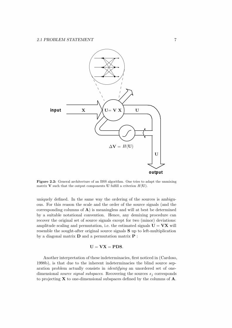
∆V = H(U)
Figure 2.2: General architecture of an BSS algorithm. One tries to adapt the unmixingmatrix V such that the output components U fulfill a criterion H(U).
uniquely defined. In the same way the ordering of the sources is ambigu-ous. For this reason the scale and the order of the source signals (and thecorresponding columns of A) is meaningless and will at best be determinedby a suitable notational convention. Hence, any demixing procedure canrecover the original set of source signals except for two (minor) deviations:amplitude scaling and permutation, i.e. the estimated signals U = VX willresemble the sought-after original source signals S up to left-multiplicationby a diagonal matrix D and a permutation matrix P :
U = VX = PDS.
Another interpretation of these indeterminacies, first noticed in (Cardoso,1998b), is that due to the inherent indeterminacies the blind source sep-aration problem actually consists in identifying an unordered set of one-dimensional source signal subspaces. Recovering the sources sj correspondsto projecting X to one-dimensional subspaces defined by the columns of A.
8 2 BLIND SOURCE SEPARATION
2.2 ICA Approach
The key concept that allows for a solution of the BSS problem is the notionof statistical independence (Jutten and Herault, 1991; Comon, 1994). Asstated above, it is assumed that the source signals sj which form the rowsof S, are statistically independent.
Intuitively, this property is important for blind source separation becausethe mixing process introduces dependencies, hence maximizing the indepen-dence is equivalent to separation. ICA tries to find the most independentcomponents of the observed data.
Popular methods for ICA are based on maximization of the output en-tropy (Bell and Sejnowski, 1995) or minimization of mutual information be-tween the outputs (Amari et al., 1996) which is in fact the minimization ofthe Kullback-Leibler divergence between the joint and the product of themarginal distributions of the outputs.
Since both approaches have been shown to be mathematical equivalent(Cardoso, 1997) to the statistical principle of maximum-likelihood estima-tion, we briefly mention the main concepts in the following subsections andpresent the maximum-likelihood approach in detail in subsection 2.2.4.
2.2.1 Statistical Independence
Statistical independence is stated mathematically in terms of the probabilitydensity function (pdf):
p(s1, . . . , sM ) =M∏
j
p(sj) (2.3)
where p(s1, . . . , sM ) denotes the joint pdf and the p(sj) denote the marginalpdf’s of the sources. In other words, for independent random variables thejoint probability distribution has a very simple form: it is just the productof the marginal distributions.
2.2.2 Characteristic Function
A related concept to assess the independence of variables is based on the socalled characteristic function. The characteristic function of an n-dimensionalrandom vector x is defined as
Φx(ω) =
∫
<p
eiωTxdF (x) = Ex{eiωT
x} (2.4)
where i =√−1 and ω is the transformed variable corresponding to x.
2.2 ICA APPROACH 9
2.2.3 Mutual Information
A well-known measure of independence of random variables is their mutualinformation (MI)1. For two random variables X and Y MI is defined as
MI(X,Y ) =
∫ ∫
dXdY logp(X,Y )
pX(X)pY (Y ).
This is the relative entropy or Kullback Leibler divergence between thejoint pdf and the product of the marginal distributions pX(X), pY (Y ). MI iszero if and only if the random variables are independent (Cover and Thomas,1991). Another name for mutual information is redundancy since the mutualinformation MI(X,Y ) can be understood as the reduction in the uncertaintyabout X given the knowledge of Y . If there is no more redundancy wehave reached independence and knowing one variable does not provide anyadditional information about the other.
2.2.4 Maximum-Likelihood Estimation
Among the approaches to solve the ICA/BSS problem, we briefly restatethe method of maximum-likelihood estimation (Pham and Garrat, 1997;Cardoso, 1997; Hyvarinen et al., 2001), because it is a fundamental methodof statistical estimation and a unique framework for a variety of algorithms.Loosely speaking, in maximum-likelihood estimation we answer the ques-tion: Given a certain probability distribution model, what is the most likelyset of parameters that would have generated the observed data?
In the language of the ICA problem, the ML principle is the following:Given the observation vector x, maximize the (log-)likelihood function ofthe mixing matrix A or, equivalently, the demixing matrix V = A−1. As afirst step we need to derive the likelihood function of the demixing matrixin the ICA model. The pdf of the observations x is:
px(x) = |detV| ps(s) (2.5)
= |detV|N∏
i=1
psi(si)
= |detV|N∏
i=1
psi(vix)
where we used the statistical independence of the marginal componentssi and the fact that 1
det A= detA−1 = detV.
We consider a fixed sample set X with T independent samples to obtainthe likelihood function:
1 MI is an important concept of information theory and has many useful properties(Cover and Thomas, 1991).

10 2 BLIND SOURCE SEPARATION
`(V) =
T∏
t=1
|detV|N∏
i=1
psi(vix) (2.6)
= (|detV|)T
T∏
t=1
N∏
i=1
psi(vix), (2.7)
where vi is the i-th row of V.
For practical optimization is preferable to use the normalized minus-log-likelihood function:
L(V) = − log `(V) = − log |detV|+ 1
T
T∑
t=1
N∑
i=1
− log psi(vix) (2.8)
Unfortunately, we can not use equation (2.8) immediately, because we donot know the pdf of the sources. Therefore one resorts to a quasi maximum-likelihood approach by choosing a specific “contrast” function h which ap-proximates the negative logarithm of the unknown source densities psi
(si).
Depending on the choice of h(·) one may only yield approximate sta-tistical independence of the variables but it can be shown that for a broadclass of functions one yields sufficient conditions to solve the BSS problem.For example, it has been shown by Zibulevsky (2003) that this approach ishighly efficient, if the sources are sparse or sparsely representable. In thiscase the absolute value function is a good choice for h(·).
Finally, we have to solve the following nonlinear optimization problem:
minV
L(V;x, h) (2.9)
Minimizing this function w.r.t. V by a suitable numerical method meansto solve the BSS problem (see Fig. 2.2).
2.3 Joint Diagonalization Approach
As pioneered by the works of Comon (1994); Molgedey and Schuster (1994);de Lathauwer (1997); Belouchrani et al. (1997); Cardoso (1999), we aim tomake use of the notion of approximate joint diagonalization (AJD) to solvethe BSS problem in a unifying framework. As the leitmotiv we want toreplace the measure of independence by a measure of diagonality of a setof matrices. This will also provide us a flexible framework for generic BSSalgorithms where the numerical optimization part can be treated efficientlyin a separate step.
2.3 JOINT DIAGONALIZATION APPROACH 11
2.3.1 From BSS to AJD
It is straightforward to see that under the assumption of the linear, instan-taneous BSS model (2.1) there exists a certain set of (unknown) “targetmatrices” which, in theory, gives rise to an joint diagonalization problem.For example, as proposed in Molgedey and Schuster (1994), we may con-sider (spatial) covariance matrices Cτ (x) of time-lagged mixed signals x(t),
Cτ (x)def= E{x(t)x(t + τ)T }
where the expectation is taken over t and τ is a time-shift parameter, wesee that the covariance of x is related to the covariance of s according to
Cτ (x) = E{(As(t))(As(t + τ))T }= A E{s(t)s(t + τ)T }AT
= ACτ (s)AT (2.10)
due to the linearity of the expectation operator and the mixing model.
The key observation is that all cross-correlation terms which are the off-diagonal elements of Cτ (s) are zero for independent signals and thus Cτ (s)is a diagonal matrix. Hence the mixing matrix A can be identified as thesolution of a matrix diagonalization problem in equation (2.10). If A isinvertible, this can also be written as
VCτ (x)VT = Cτ (s) = Dτ , (2.11)
where the matrix V = A−1 is diagonalizing all Cτ (x) simultaneously. Inpractice, the target matrices Cτ (x) have always to be estimated from theavailable data with a finite sample size T . Typically the expectation iscomputed as a sample average
Cτ (x)def=
1
T
T−τ∑
t=1
(x(t)x(t + τ)T
). (2.12)
It is clear that this procedure inevitably gives rise to estimation errors, how-ever, the pragmatic approach is to assume that these errors can be neglectedfor sufficiently large T . Thus for large T we conclude analogously to (2.10)that
Cτ (x) = ACτ (s)AT .
This means that the BSS problem has been translated into an equivalentproblem of approximate joint diagonalization.
12 2 BLIND SOURCE SEPARATION
2.3.2 Symmetrizing
We note that the matrices Cτ (x) are not symmetric by construction, howeverit is appropriate to symmetrize them, because under the ICA model the anti-symmetric part is assumed to be zero and thus the diagonalization problemcan be fully based on the symmetric part of Cτ (x):
(Cτ (x) + Cτ (x)T ) = A (Cτ (s) + Cτ (s)T )
︸ ︷︷ ︸
↓
AT (2.13)
V (Cτ (x) + Cτ (x)T ) VT = Dτ (2.14)
2.3.3 A Two-Stage Algorithm
From (2.14) we conclude that finding a transformation matrix V whichdiagonalizes the estimated, symmetrized target set “as good as possible”provides us an estimate of the demixing matrix.
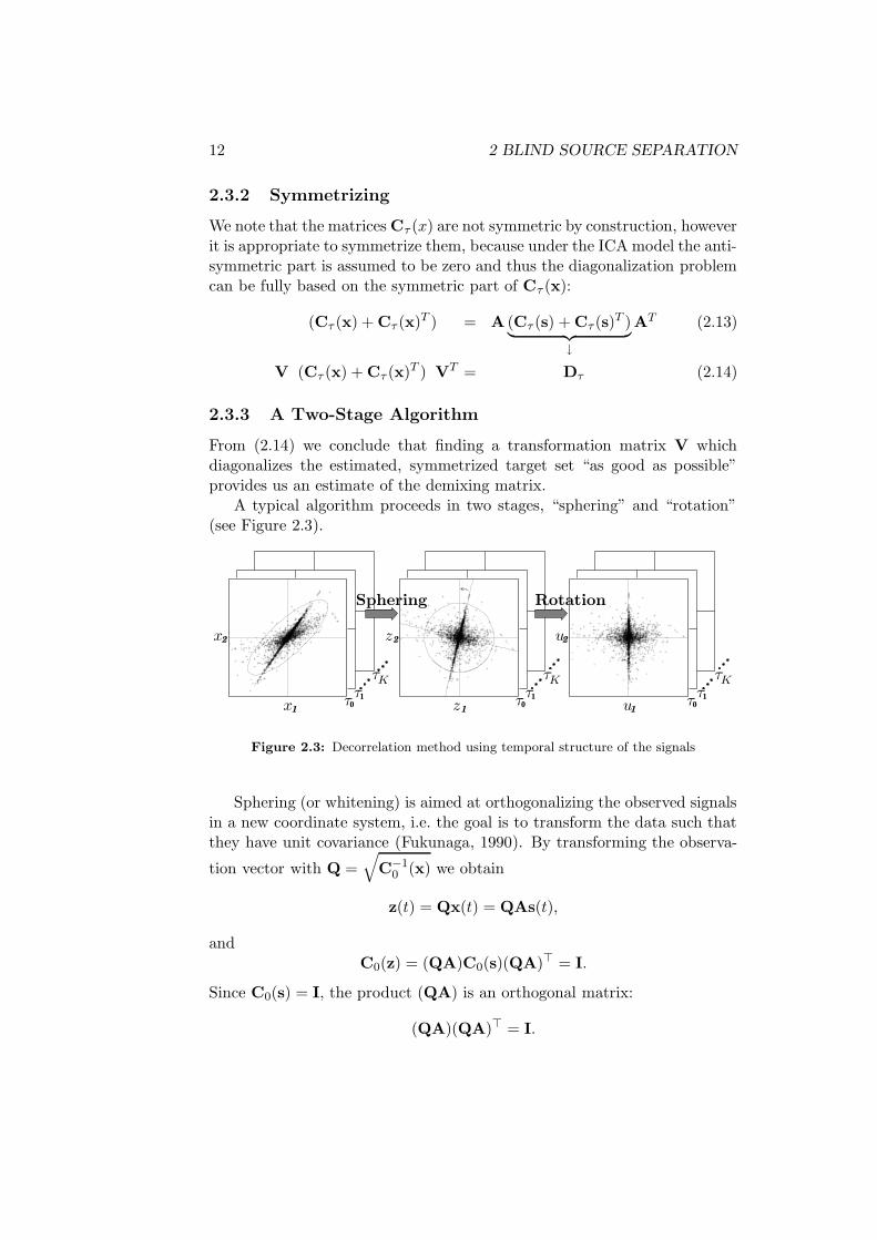
A typical algorithm proceeds in two stages, “sphering” and “rotation”(see Figure 2.3).
01
01
01
1
2
11
22
PSfrag replacements
τττ
τττ
τττ
x
x
u
u
z
z
KKK
RotationSphering
Figure 2.3: Decorrelation method using temporal structure of the signals
Sphering (or whitening) is aimed at orthogonalizing the observed signalsin a new coordinate system, i.e. the goal is to transform the data such thatthey have unit covariance (Fukunaga, 1990). By transforming the observa-
tion vector with Q =√
C−10 (x) we obtain
z(t) = Qx(t) = QAs(t),
andC0(z) = (QA)C0(s)(QA)> = I.
Since C0(s) = I, the product (QA) is an orthogonal matrix:
(QA)(QA)> = I.
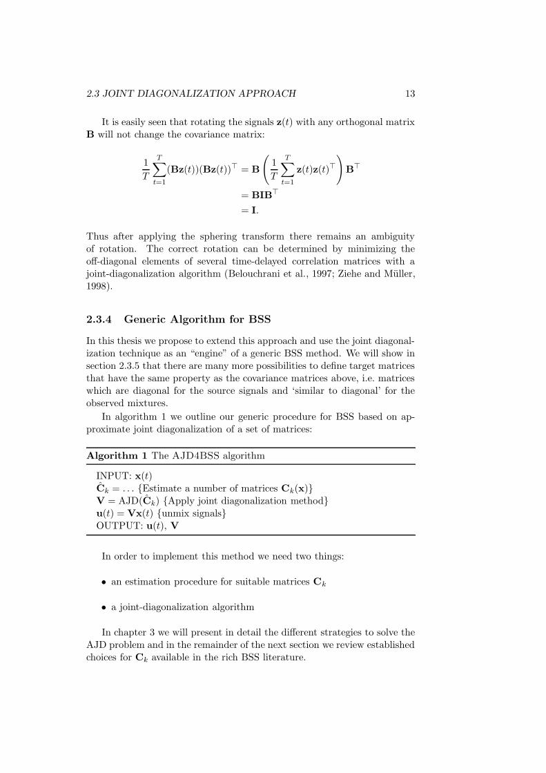
2.3 JOINT DIAGONALIZATION APPROACH 13
It is easily seen that rotating the signals z(t) with any orthogonal matrixB will not change the covariance matrix:
1
T
T∑
t=1
(Bz(t))(Bz(t))> = B
(
1
T
T∑
t=1
z(t)z(t)>)
B>
= BIB>
= I.
Thus after applying the sphering transform there remains an ambiguityof rotation. The correct rotation can be determined by minimizing theoff-diagonal elements of several time-delayed correlation matrices with ajoint-diagonalization algorithm (Belouchrani et al., 1997; Ziehe and Muller,1998).
2.3.4 Generic Algorithm for BSS
In this thesis we propose to extend this approach and use the joint diagonal-ization technique as an “engine” of a generic BSS method. We will show insection 2.3.5 that there are many more possibilities to define target matricesthat have the same property as the covariance matrices above, i.e. matriceswhich are diagonal for the source signals and ‘similar to diagonal’ for theobserved mixtures.
In algorithm 1 we outline our generic procedure for BSS based on ap-proximate joint diagonalization of a set of matrices:
Algorithm 1 The AJD4BSS algorithm
INPUT: x(t)Ck = . . . {Estimate a number of matrices Ck(x)}V = AJD(Ck) {Apply joint diagonalization method}u(t) = Vx(t) {unmix signals}OUTPUT: u(t), V
In order to implement this method we need two things:
• an estimation procedure for suitable matrices Ck
• a joint-diagonalization algorithm
In chapter 3 we will present in detail the different strategies to solve theAJD problem and in the remainder of the next section we review establishedchoices for Ck available in the rich BSS literature.
14 2 BLIND SOURCE SEPARATION
2.3.5 Possible Target Matrices
In this section we catalog different choices for the set of target matrices.The main purpose is to give a “cookbook- like” overview how particularproperties of the involved signals are used to construct such matrices fromthe data and to show the connection to existing BSS algorithms.
Historically, the suitability of joint diagonalization criteria as BSS costfunctions have been realized by several authors. Pioneered in the earlyworks of Tong et al. (1991); Comon (1994); Molgedey and Schuster (1994);Matsuoka et al. (1995); Laheld and Cardoso (1996); Belouchrani et al. (1997)related methods emerged in articles of Wu and Principe (1999); Hori (1999);Pham and Cardoso (2001); Yeredor (2002). Interestingly, all of the “threeeasy routes” to ICA pointed out in Cardoso (2001) have analogous specificdefinitions of the set of target matrices {C1,C2, . . . ,CK}. The basic idea isto exploit certain ‘non–properties’ of the signals. The three most often usedproperties of this kind are:
• non-Gaussianity
• non-Stationarity
• spectral non-Flatness
Non-Gaussianity
If we assume that the source processes si(t) are independent identically dis-tributed, the BSS method has to rely on the non-Gaussianity of the sources.Non-Gaussianity means that the source density is sufficiently different froma Gaussian density. The key point is that by mixing the signals become moreand more Gaussian, since the distribution of the sum of many independentrandom variables tends to be Gaussian (Hyvarinen et al., 2001).
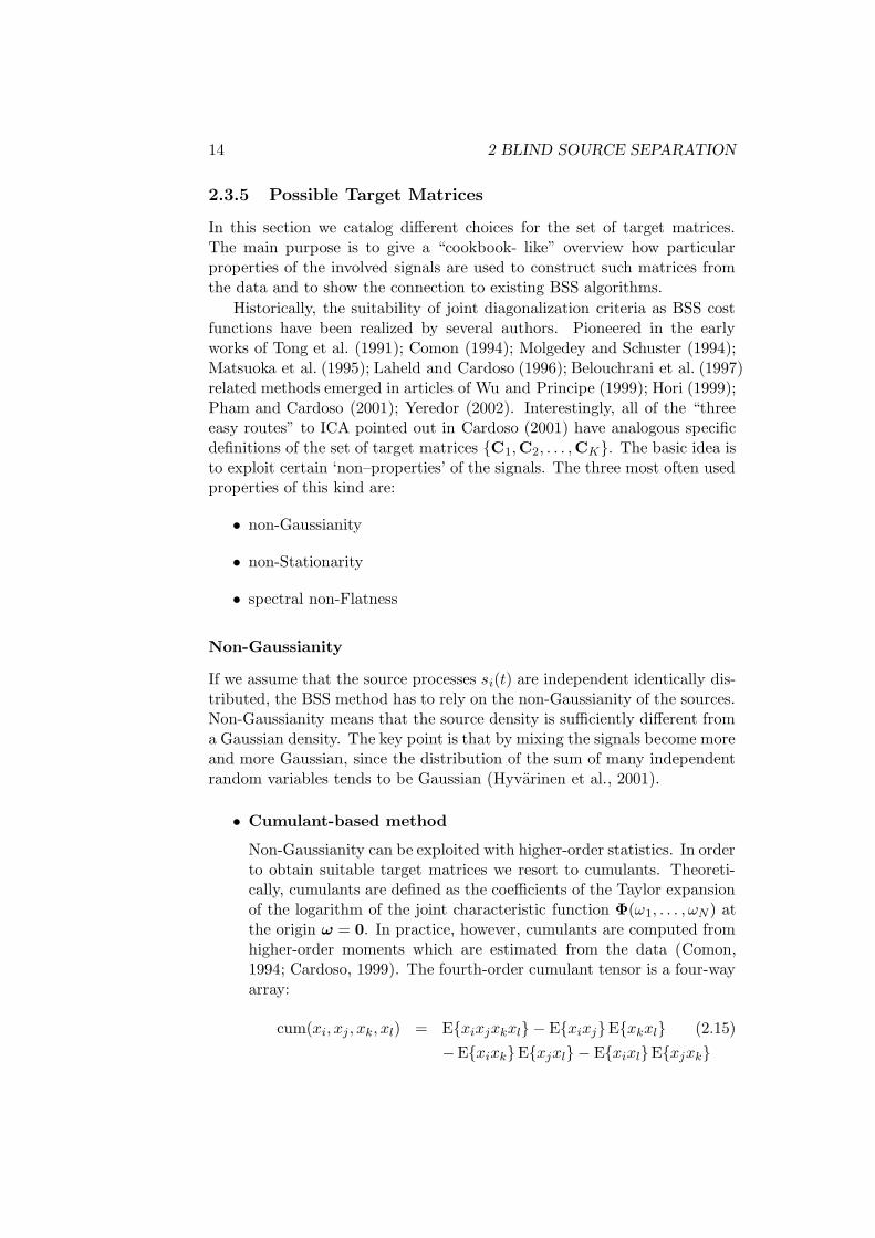
• Cumulant-based method
Non-Gaussianity can be exploited with higher-order statistics. In orderto obtain suitable target matrices we resort to cumulants. Theoreti-cally, cumulants are defined as the coefficients of the Taylor expansionof the logarithm of the joint characteristic function Φ(ω1, . . . , ωN ) atthe origin ω = 0. In practice, however, cumulants are computed fromhigher-order moments which are estimated from the data (Comon,1994; Cardoso, 1999). The fourth-order cumulant tensor is a four-wayarray:
cum(xi, xj , xk, xl) = E{xixjxkxl} − E{xixj}E{xkxl} (2.15)
−E{xixk}E{xjxl} − E{xixl}E{xjxk}
2.3 JOINT DIAGONALIZATION APPROACH 15
The matrices to be diagonalized can be obtained from ‘parallel slices’of the fourth-order cumulant tensor:
C(ij)(M) =∑
kl
M(kl) cum(xi, xj, xk, xl), (2.16)
where M is an arbitrary matrix (see also Hyvarinen et al. (2001)).
The popular JADE2 algorithm (Cardoso and Souloumiac, 1993) be-longs to this class. After whitening the data, JADE performs an ap-proximate diagonalization of the set of eigen-matrices of the cumulanttensor with an orthogonal transformation composed of a sequence ofplane rotations (Cardoso and Souloumiac, 1993; Comon, 1994).
The plane rotation R(θ; i, j) is defined as the identity matrix wherethe (i, i) and (j, j) entries are replaced by cos(θ) and the (i, j) entry isreplaced by − sin(θ) and the (j, i) entry is replaced by sin(θ) . Thenfor each pair (i, j) one computes the optimal angle θ which mininizesthe cost function.
Due to the high computational load for storing and processing thefourth-order order cumulants the application of this method often re-quires a dimension reduction.
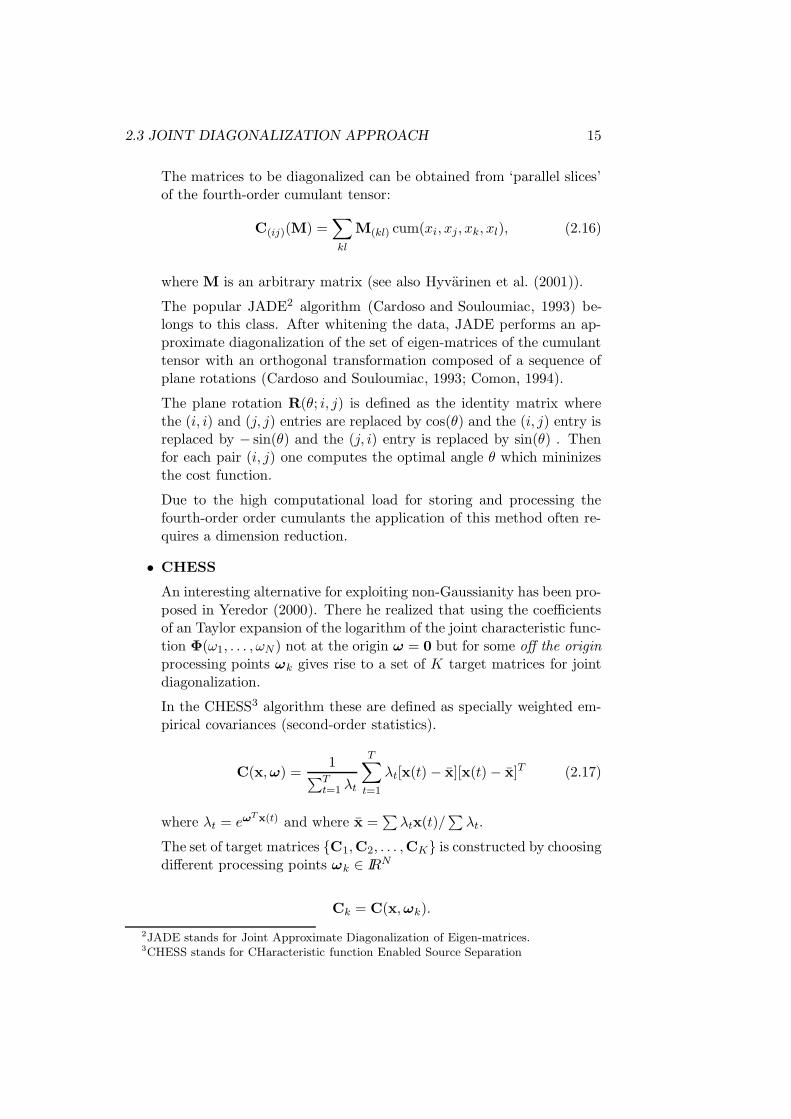
• CHESS
An interesting alternative for exploiting non-Gaussianity has been pro-posed in Yeredor (2000). There he realized that using the coefficientsof an Taylor expansion of the logarithm of the joint characteristic func-tion Φ(ω1, . . . , ωN ) not at the origin ω = 0 but for some off the originprocessing points ωk gives rise to a set of K target matrices for jointdiagonalization.
In the CHESS3 algorithm these are defined as specially weighted em-pirical covariances (second-order statistics).
C(x,ω) =1
∑Tt=1 λt
T∑
t=1
λt[x(t) − x][x(t)− x]T (2.17)
where λt = eωT x(t) and where x =
∑λtx(t)/
∑λt.
The set of target matrices {C1,C2, . . . ,CK} is constructed by choosingdifferent processing points ωk ∈ IRN
Ck = C(x,ωk).
2JADE stands for Joint Approximate Diagonalization of Eigen-matrices.3CHESS stands for CHaracteristic function Enabled Source Separation

16 2 BLIND SOURCE SEPARATION
The advantage of this method is that the induced computational loadand the statistical robustness are more favorable than for the abovecumulant method.
Non-Stationarity
The i.i.d.assumption is often too restrictive and it is useful to exploit possibletemporal structure. Then we can even recover Gaussian sources. A verysimple form of temporal structure is related to non-stationarity. Here weassume that the variance σ2 of the sources is not constant over time, butvaries according to some “amplitude profile” σ(t). Furthermore the variationis assumed to be relatively slow. Thus we rely on the following properties:
• signals are supposed to be stationary within a short time-scale,
• and signals are intrinsically non-stationary over the long run.
In this case the set of target matrices is constructed from the empiricalcovariance matrix in different segments of the data (Matsuoka et al., 1995;Pham and Garrat, 1997; Parra and Spence, 2000; Pham and Cardoso, 2000,2001; Choi et al., 2001).
Non-Flatness
The second case of non-i.i.d.sources originates from time dependencies. Thesedata exhibit broad band power spectra that are not constant over the fre-quencies (non-flat spectra).
It is interesting to note that most ’natural’ signals, like speech signalsor neurophysiological signals (EEG, MEG, etc.) have a rich dynamical timestructure. Hence we want to directly exploit their diversity in the time-frequency domain for blind source separation.
Examples for possible target matrices in this class are time-lagged covari-ances (cf. Tong et al., 1991; Molgedey and Schuster, 1994; Belouchrani et al.,1997; Ziehe and Muller, 1998), where the respective auto– and cross–correlationfunctions φxi,xj
(τ) = E{xi(t)xj(t− τ)} in are arranged in matrix form:
Cτ (x) =
φx1,x1(τ) · · · φx1,xN(τ)
φx2,x1(τ) · · · φx2,xN(τ)
.... . .
...φxN ,x1(τ) · · · φxn,xN
(τ)
. (2.18)
In (Ziehe et al., 2000b), the Ck are defined as:
Ck(x) =1
T
T∑
t=1
x(t) (hk ? x(t))T , (2.19)
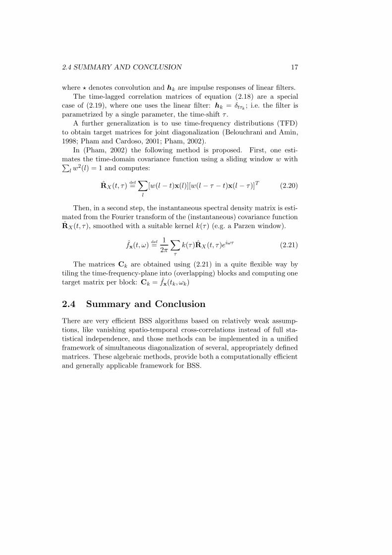
2.4 SUMMARY AND CONCLUSION 17
where ? denotes convolution and hk are impulse responses of linear filters.The time-lagged correlation matrices of equation (2.18) are a special
case of (2.19), where one uses the linear filter: hk = δtτk; i.e. the filter is
parametrized by a single parameter, the time-shift τ .A further generalization is to use time-frequency distributions (TFD)
to obtain target matrices for joint diagonalization (Belouchrani and Amin,1998; Pham and Cardoso, 2001; Pham, 2002).
In (Pham, 2002) the following method is proposed. First, one esti-mates the time-domain covariance function using a sliding window w with∑
l w2(l) = 1 and computes:
RX(t, τ)def=∑
l
[w(l − t)x(l)][w(l − τ − t)x(l − τ)]T (2.20)
Then, in a second step, the instantaneous spectral density matrix is esti-mated from the Fourier transform of the (instantaneous) covariance functionRX(t, τ), smoothed with a suitable kernel k(τ) (e.g. a Parzen window).
fx(t, ω)def=
1
2π
∑
τ
k(τ)RX (t, τ)eiωτ (2.21)
The matrices Ck are obtained using (2.21) in a quite flexible way bytiling the time-frequency-plane into (overlapping) blocks and computing onetarget matrix per block: Ck = fx(tk, ωk)
2.4 Summary and Conclusion
There are very efficient BSS algorithms based on relatively weak assump-tions, like vanishing spatio-temporal cross-correlations instead of full sta-tistical independence, and those methods can be implemented in a unifiedframework of simultaneous diagonalization of several, appropriately definedmatrices. These algebraic methods, provide both a computationally efficientand generally applicable framework for BSS.

18 2 BLIND SOURCE SEPARATION
Chapter 3
Approximate Joint
Diagonalization of Matrices
In this chapter we address the problem of approximate jointdiagonalization (AJD) of several real-valued, symmetric ma-trices. In the previous chapter (section 2.3) we have seen thatAJD provides a general framework for handling generic BSSproblems. In the following sections, we introduce the jointdiagonalization concept and derive new, computationally ef-ficient algorithms implementing these ideas. This chapter ismainly based on the publications (Ziehe et al., 2003c, 2004)and (Yeredor, Ziehe and Muller, 2004).
3.1 Introduction
Joint diagonalization of square matrices is an important general problemof numeric computation. Besides other applications, joint diagonalizationtechniques provide a generic algorithmic tool for blind source separation. Inthis chapter the joint diagonalization problem is formulated and state-of-the-art approaches for its solution are reviewed.
The main part of this chapter is devoted to the derivation of new al-gorithms to efficiently perform a joint diagonalization of several symmetricmatrices. The general structure of these algorithms will be based on a multi-plicative update with a matrix exponential in order to constrain the solutionto a particular manifold. We will see that the use of such matrix exponentialupdate enables the development of efficient optimization algorithms.
Before we come to the joint diagonalization problem we recall some basicfacts from linear algebra.
19

20 3 APPROXIMATE JOINT DIAGONALIZATION OF MATRICES
Eigenvalues, Eigenvectors, Diagonalization
A matrix D is diagonal if Dij = 0 whenever i 6= j.The notion of diagonalizing a matrix M is closely related to solving an
eigenvalue problem. In matrix form the eigenvalue problem is: Given anN ×N matrix M, find a N ×N matrix E and a diagonal N ×N matrix D,such that
ME = ED. (3.1)
If M is symmetric and real-valued, then a solution always exists whereE is an orthogonal matrix (i.e. EET = I) consisting of the eigenvectors andthe diagonal elements of D are the eigenvalues of M.
Thus writing M = EDET , where E is orthogonal and D is diagonal,gives a factorization known as the eigenvalue decomposition (EVD).
Generalized Eigenvalue Problem
Also for two normal matrices, it is well known that exact joint diagonal-ization is possible and is referred to as the generalized eigenvalue problem:Given two N × N matrices M1 and M2, find a N × N matrix E and adiagonal N ×N matrix D, such that
M1E = M2ED. (3.2)
If M2 is non-singular, the problem (3.2) can be reduced to problem(3.1) by multiplying (3.2) from the left with M−1
2 . Extensive literatureexists on this topic (e.g. Noble and Daniel, 1977; Golub and van Loan, 1989;Bunse-Gerstner et al., 1993; Vorst and Golub, 1997, and references therein).
Approximate Joint Diagonalization
In general, it is not possible to diagonalize more than two matrices with onesingle transformation. However, exact diagonalization of more than two ma-trices is possible if the matrices possess a certain common structure, as it isthe case for the blind source separation application (see e.g. equation (2.11)) . If the ideal model of equation (2.11) holds, exact joint diagonalization ispossible, otherwise, one can only speak of approximate joint diagonalization(AJD). In the remainder of the chapter we will use the terms “approximatejoint diagonalization” and “joint diagonalization” interchangeably for diag-onalization of more than two matrices with a single transformation. Theapproximation is understood in the sense of minimizing a suitable diagonal-ity criterion.
Many algorithms for joint diagonalization have been previously proposed(e.g. Flury and Gautschi, 1986; Cardoso and Souloumiac, 1993, 1996; Hori,1999; Pham, 2001; van der Veen, 2001; Yeredor, 2002; Joho and Rahbar,2002).
3.2 SOLVING THE JOINT DIAGONALIZATION PROBLEM 21
In order to better understand the challenges of AJD and to explorepossible directions to improve the existing algorithms, we first study someexisting approaches to solve the joint diagonalization problem.
3.2 Solving the Joint Diagonalization Problem
3.2.1 Three Cost Functions
In this section we consider the approximate joint diagonalization of a of real-valued symmetric matrices of size N×N .1 The goal of a joint diagonalizationalgorithm is to find a matrix V that simultaneously transforms C1, . . . ,CK
as good as possible to diagonal form. The notion of closeness to diagonalityand the corresponding formal statement of the joint diagonalization problemcan be defined in different ways:
1. Subspace fitting formulation.
Approximate joint diagonalization consists of the following optimiza-tion problem (van der Veen, 2001; Yeredor, 2002): Given a set of KN ×N “target matrices” C1,C2, . . . ,CK , find a N ×N matrix A andK diagonal matrices D1,D2, . . . ,DK such that the following quantityis minimized:
J1(A,D1,D2, . . . ,DK) =
K∑
k=1
||Ck −ADkAT ||2F (3.3)
where || · || denotes the squared Frobenius norm.
2. Frobenius norm formulation.
This formulation of the joint diagonalization problem has been usedmost frequently in the literature, e.g. in Bunse-Gerstner et al. (1993);Cardoso and Souloumiac (1993, 1996); Hori (1999); Joho and Rahbar(2002); Joho and Mathis (2002). Here, the goal is to find the inverseV = A−1 of the matrix A, by minimizing the diagonality criterion:
J2(V) =
K∑
k=1
off(VCkVT ) (3.4)
where the off(·) is the Frobenius norm of the off-diagonal elements,
off(M)def= ||M− diag(M)||2F =
∑
i6=j
(Mij)2. (3.5)
1The formulations and the proposed algorithms will be presented for real-valued, sym-metric matrices only. We note however, that extensions to the complex-valued case couldbe obtained in a similar manner.
22 3 APPROXIMATE JOINT DIAGONALIZATION OF MATRICES
While the diagonality measure (3.5) appears very natural and intuitive,the cost function (3.4) has the disadvantage that the Frobenius normis obviously minimized by the trivial solution V = 0. Therefore anoptimization method with an additional constraint to exclude the zerosolution is required.
3. Positive definite formulation. Often it is reasonable to assume thatin the initial problem all the matrices Ck are positive-definite. Thisassumption is motivated by the fact that in many applications matricesCk are covariance matrices of some random variables. In this case, asproposed in Matsuoka et al. (1995); Pham (2001) the criterion
J3(V)def= log det(diag(VCkV
T ))− log det(VCkVT ) (3.6)
can be used instead of the cost function (3.5). Here the operatordiag(M) returns a diagonal matrix containing only the diagonal entriesof M.
This measure can be traced back to information theory as the Kullback-Leibler distance between a Gaussian process with covariance matrixC and its diagonal part diag(C). The additional advantage of thiscriterion is its scale invariance (Pham and Cardoso, 2001).
However, in certain applications, the matrices are not always guar-anteed to be positive-definite. For example in blind source sepa-ration based on time-delayed decorrelation (Belouchrani et al., 1997;Ziehe and Muller, 1998), correlations can be positive or negative andin this case the criterion J3 can not be used.
Compared to the approaches 2. and 3., the algorithms based on subspacefitting have two advantages: they do not require orthogonality, positive-definiteness or any other normalizing assumptions on the matrices A andCk, and they are able to handle non-square mixture matrices. These ad-vantages, however, come at the price of a high computational cost: thealgorithm of van der Veen (2001) has quadratic convergence in the vicinityof the minimum, but its running time per iteration is O(KN 6); the AC-DC algorithm of Yeredor (2002) converges linearly with a running time periteration of order O(KN 3).
The algorithms relying on the positive-definiteness assumption are alsoefficient thanks to the favorable invariance properties, but they fail for non-positive-definite matrices. Least-squares subspace fitting algorithms, whichdo not require such strong a-priori assumptions, are computationally muchmore demanding. Our work is motivated by the question: could we developa method that combines all the good features and at the same time avoidsthe shortcomings of the previous joint diagonalization algorithms?

3.2 SOLVING THE JOINT DIAGONALIZATION PROBLEM 23
3.2.2 Our Approach
In our approach we want to employ the Frobenius off-diagonal norm for-mulation and minimize the cost function J2. For this we have to solvea constrained non-linear optimization problem, i.e. essentially a quadraticleast-squares problem with an constraint that prevents the algorithm fromconverging to the trivial solution.
One of the standard algorithms for solving nonlinear least-squares prob-lems is for example the Levenberg-Marquardt (LM) algorithm (Levenberg,1944; Marquardt, 1963). However, the LM algorithm cannot be directlyapplied to our problem, because the classical LM algorithm does not pro-vide means for incorporation of additional constraints, such as orthogonalityor invertibility of the diagonalizer V. In what follows we present a differ-ent strategy how to cope with the constrained optimization problem whichnaturally incorporates the additional structure of our problem into the al-gorithm.
The key point is to make use of matrix exponential updates and to exploitthe fact that our parameter space consists of the group of orthogonal, ormore general, invertible matrices.
3.2.3 General Structure of Our Algorithm
Our goal is to solve the following constrained non-linear optimization prob-lem:
minV
K∑
k=1
∑
i6=j
((VCkVT )ij)
2. (3.7)
Due to the non-linearity of the problem, we can not obtain a solution forV in closed form. Instead we have to use an iterative scheme to successivelyimprove an initial solution. The main problem with this approach is howeverto avoid the trivial solution V = 0 which poses a constraint to (3.7).
In the traditional approach one would introduce a penalty term whichhas a minimum when an additional normalization constraint is satisfied. Forexample, Joho and Rahbar (2002) proposed to use:
J4 = ||VVT − I||F (3.8)
J5 = ||diag(V − I)||F (3.9)
In contrast, we prefer to use the group structure of the search space as ahard constraint preventing convergence of the minimizer of the cost functionin Equation (3.7) to the zero solution.
We propose the following iterative process. We start with a matrix V(0)
that belongs to the group and carry out multiplicative updates:
V(m+1) ← exp(W(m+1))V(m), (3.10)
24 3 APPROXIMATE JOINT DIAGONALIZATION OF MATRICES
where exp(·) denotes the matrix exponential and V(m+1) the estimated di-agonalizing (demixing) matrix after the (m+1)-th iteration (see Figure 3.1).The new parameter W(m+1) of the update multiplier is to be determined soas to minimize the cost function (3.7).
For the update it is also important that the matrix V(m+1) remainsalways within the group manifold. This can be ensured by certain conditionson W(m+1) and will be discussed in subsection 3.2.4.
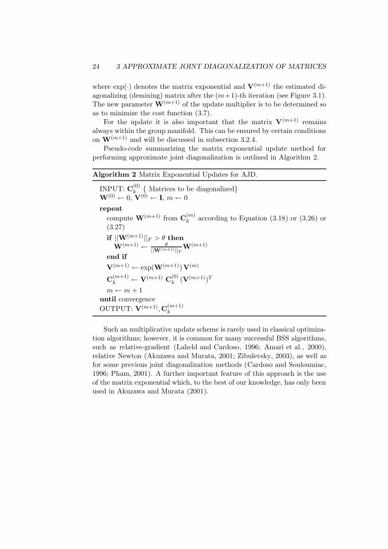
Pseudo-code summarizing the matrix exponential update method forperforming approximate joint diagonalization is outlined in Algorithm 2.
Algorithm 2 Matrix Exponential Updates for AJD.
INPUT: C(0)k { Matrices to be diagonalized}
W(0) ← 0, V(0) ← I, m← 0
repeat
compute W(m+1) from C(m)k according to Equation (3.18) or (3.26) or
(3.27)
if ||W(m+1)||F > θ thenW(m+1) ← θ
||W(m+1)||FW(m+1)
end if
V(m+1) ← exp(W(m+1))V(m)
C(m+1)k ← V(m+1) C
(0)k (V(m+1))T
m← m + 1until convergence
OUTPUT: V(m+1),C(m+1)k
Such an multiplicative update scheme is rarely used in classical optimiza-tion algorithms; however, it is common for many successful BSS algorithms,such as relative-gradient (Laheld and Cardoso, 1996; Amari et al., 2000),relative Newton (Akuzawa and Murata, 2001; Zibulevsky, 2003), as well asfor some previous joint diagonalization methods (Cardoso and Souloumiac,1996; Pham, 2001). A further important feature of this approach is the useof the matrix exponential which, to the best of our knowledge, has only beenused in Akuzawa and Murata (2001).

3.2 SOLVING THE JOINT DIAGONALIZATION PROBLEM 25
3.2.4 Structure Preserving Updates
In order to derive algorithms that take the group structure of our parameterspace into account, we consider repeated multiplicative updates (see Figures3.3 and 3.1). The fundamental concept is the matrix exponential function.
The Exponential Map
The exponential of a real valued square matrix M, denoted by eM orexp(M), is defined as
eM = exp(M) =
∞∑
k=0
1
k!Mk (3.11)
= I + M +M2
2!+ . . .
The matrix exponential satisfies the following properties:
1. For the N ×N zero matrix O, e0 = I, where I is the N ×N identitymatrix.
2. If M = Q
D1
. . .
DN
Q−1 for an invertible N × N matrix Q,
then eM = Q
eD1
. . .
eDN
Q−1.
3. If M′ is a matrix of the same type as M, and M and M′ commute,then eM+M
′
= eMeM′
.
4. The trace of M and the determinant of eM are related by the formuladet eM = etrM. Therefore eM is always invertible and the inverse is(eM)−1 = e−M.
In applications of approximate joint diagonalization to the BSS problemwe are mainly interested in two special cases where the transformation V isassumed to be:
• orthogonal, i.e. V ∈ O(N) or
• invertible, i.e. V ∈ GL(N).
The multiplicative matrix exponential update preserves these importantfeatures, because the product of orthogonal (invertible) matrices is an or-thogonal (invertible) matrix.

26 3 APPROXIMATE JOINT DIAGONALIZATION OF MATRICES
G
matrix Lie group
PSfrag replacements
WV(m)
V(m+1)=eWV(m)
Lie group
tangent space
eW
log
L
T GV(m)
T GI
0
Figure 3.1: Illustration of multiplicative updates using the matrix exponential map: alocal step in the tangent space is mapped to a distinct point on the manifold.
Orthogonal case
The most popular structural assumption is orthogonality of V. In fact,such an assumption seems natural if the joint diagonalization problem isseen as an extension of the eigenvalue problem and one asks for the commonorthogonal basis of several matrices.
A further reason for the importance of this special case is the fact thatwe can use a sphering step as a pre-processing (see also section 2.3.3). Thesphering can be done as follows: First, we pick one positive-definite sym-metric matrix C from the setM. Then, the sphering transform Q is definedby the matrix that is obtained as the inverse square root of C.
This matrix can be computed via the eigenvalue decomposition of C,C = EDET , which implies:
Qdef= C− 1
2 = (EDET )−12 = ED− 1
2 ET .
To see that this is indeed a sphering transformation, we apply Q = C− 12 to
C = EDET , where E is orthogonal. This yields
QCQT = ED− 12 ETEDETED− 1
2 ET = I.
This transformation is illustrated in Fig. 3.2 for a 2× 2 positive-definitematrix.
In general, the simultaneously diagonalizable matrices Ck can be writtenin the form ADkA
T , where A is a non-orthogonal invertible matrix and Dk
are diagonal matrices. Applying the sphering transform to Ck = ADk AT
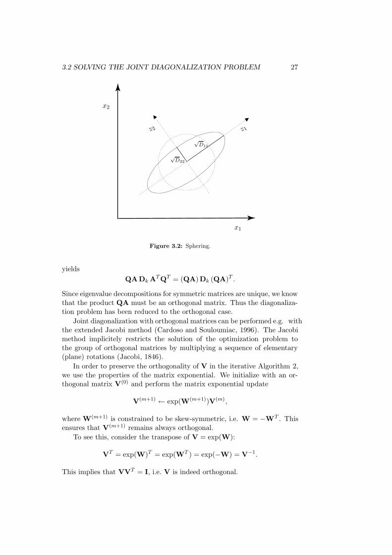
3.2 SOLVING THE JOINT DIAGONALIZATION PROBLEM 27
PSfrag replacements
x1
x2
z1
√D11
√D22
z 2
Figure 3.2: Sphering.
yields
QADk ATQT = (QA)Dk (QA)T .
Since eigenvalue decompositions for symmetric matrices are unique, we knowthat the product QA must be an orthogonal matrix. Thus the diagonaliza-tion problem has been reduced to the orthogonal case.
Joint diagonalization with orthogonal matrices can be performed e.g. withthe extended Jacobi method (Cardoso and Souloumiac, 1996). The Jacobimethod implicitely restricts the solution of the optimization problem tothe group of orthogonal matrices by multiplying a sequence of elementary(plane) rotations (Jacobi, 1846).
In order to preserve the orthogonality of V in the iterative Algorithm 2,we use the properties of the matrix exponential. We initialize with an or-thogonal matrix V(0) and perform the matrix exponential update
V(m+1) ← exp(W(m+1))V(m),
where W(m+1) is constrained to be skew-symmetric, i.e. W = −WT . Thisensures that V(m+1) remains always orthogonal.
To see this, consider the transpose of V = exp(W):
VT = exp(W)T = exp(WT ) = exp(−W) = V−1.
This implies that VVT = I, i.e. V is indeed orthogonal.

28 3 APPROXIMATE JOINT DIAGONALIZATION OF MATRICES
Non-Orthogonal case
The algorithm 2 can also be used in the non-orthogonal case. Here we wantto employ the constraint that V has to be an invertible (non-singular) ma-trix. Mathematically this condition means detV 6= 0. Due to the propertiesof the matrix exponential this is always guaranteed, since det(eW) = etrW
and the exponential function is always non-zero.
Additionally, we may enforce V to be volume-preserving, i.e. det(V) = 1.Based on the following fact, which is also a consequence of the relationdet(eW) = etrW for the matrix exponential, this can be done by setting thetrace of W to zero:
Theorem (volume preservation). If trW = 0, then det(eW) = 1.
This means that the mutltiplicative update V(m+1) ← exp(W(m+1))V(m),with trW = 0, preserves the determinant. If we start with a matrix V0,where detV0 = 1, this ensures det(V(m)) = 1,∀m.
However the exact matrix exponential is relativly expensive to compute(O(N3)) and thus one may want to use a computationally cheaper first-order approximation eW ≈ I + W (see Figure 3.3). In order to maintaininvertibility of V when using a such a first-order approximation, it suffices toensure invertibility of I+W. For this purpose we can resort to the followingresults of matrix analysis (Horn and Johnson, 1985).
Definition. An N ×N matrix M is said to be strictly diagonally dominantif
|Mii| >∑
j 6=i
|Mij |, for all i = 1, . . . , N.
Theorem (Levi-Desplanques). If an N×N matrix M is strictly diagonally-dominant, then it is invertible.
With M = I+W the Levi-Desplanques theorem helps us to control theinvertibility of I + W. We notice that the diagonal entries in I + W are allequal to 1; therefore, it suffices to ensure that
1 > maxi
∑
j 6=i
|Wij | = ||W||∞.
This can be done by scaling W by its infinity norm ||W||∞ whenever thelatter exceeds some fixed threshold θ < 1. An even stricter condition can beimposed by using a Frobenius norm ||W||F in the same way:
W← θ
||W||FW. (3.12)

3.2 SOLVING THE JOINT DIAGONALIZATION PROBLEM 29
PSfrag replacements
V(1) = eW(1)
eW(2)
eW(3)
(I + W(1))
(I + W(2))(I + W(3))
I
Figure 3.3: The (matrix) exponential can be approximated by I + W for small W.
3.2.5 Discussion
In principle, a restriction of V to the group of orthogonal matrices canbe used if at least one matrix of the set of target matrices happens to bepositive-definite. In this case, the pre-sphering step can be applied. We notehowever that such a two step method may degrade the overall performance,because one (arbitrary) matrix of the set is diagonalized exactly at the ex-pense of a worse diagonalization of the remaining matrices. This can beespecially problematic in the context of blind source separation (Cardoso,1994; Yeredor, 2002; Akuzawa and Murata, 2001). Thus we want to relaxthe orthogonality assumption and consider the case of approximate jointdiagonalization with non-orthogonal matrices. In the non-orthogonal casehowever, we additionally need enforce some constraint to prevent trivialsolutions. Here we make use of the invertibility of V which is implicitlyguaranteed when using the multiplicative matrix exponential update. In-vertibility is a inherent necessity in many applications of diagonalizationalgorithms, especially in blind source separation, therefore making use ofsuch a constraint is very natural and does not limit the usefulness from thepractical point of view.
The cost of computing the matrix exponential are O(N 3), which is rel-atively high, but since for typical BSS problems the dimensionality of the

30 3 APPROXIMATE JOINT DIAGONALIZATION OF MATRICES
matrices is of the order N ≈ 100 it is by no means computational prohibitive.A computationally cheaper alternative to the exact matrix exponential up-date is to use a first-order approximation exp(W) ≈ I + W for sufficientlysmall W.
3.3 Computation of the Update Matrix
In this section we are going to derive the update rules for the matrix W(m+1)
such that we actually minimize our joint diagonality criterion. We will con-sider two approaches: a gradient method, called DOMUNG (Yeredor, Zieheand Muller, 2004) and a Newton-like method, called FFDiag (Ziehe et al.,2003c, 2004).
3.3.1 Relative Gradient Algorithm: DOMUNG
Throughout the following derivations the operation of setting the diagonalof a matrix to zero is frequently used. Thus we denote this operation byputting an upper bar above the respective expression. More specifically, forany square matrix M we define the notation M as
Mdef= M− diag(M) (3.13)
Note that the off(·) operator defined in (3.5) can then be expressed basedon the trace of a matrix:
off(M) = ||M||2F = tr{MTM} = tr{MT M}. (3.14)
To determine the updates W at each iteration, first-order optimalityconstraints for the objective (3.7) are used. We may therefore define, foreach iteration m,
J(m)2 (W)
def=
K∑
k=1
off((I + W)C(m)k (I + W)T ), (3.15)
as the cost function which we seek to minimize w.r.t. W. To this end, we
now seek the gradient ∂J(m)2 (W)/∂W, which is a matrix whose (i, j)-th
element is the derivative of J(m)2 (W) w.r.t. Wij (Wij denoting the (i, j)-th
element of W). To find this gradient matrix, we first compute the gradientof each summand in (3.15). We do so by expressing the off(·) function in(3.15) in the vicinity of W = 0 up to first-order terms in W, i.e. we assumethat W is a sufficiently small matrix (for shorthand we omit the indices in
3.3 COMPUTATION OF THE UPDATE MATRIX 31
the following expressions, i.e. we use C instead of C(m)k ):
off((I + W)C(I + W)T ) = tr{[(I + W)C(I + W)T ]T (I + W)C(I + W)T
= tr{(I + W)C(I + W)T (I + W)C(I + W)T }≈ tr{(C + WC + CWT )(C + WC + CWT )}≈ tr{CC + CWC + CCWT + WCC + CWTC}
˜J2(W) = tr{CC + CCW + CCW + CCW + CCW}= tr{CC}+ 4 tr{CCW}. (3.16)
We used (3.14) in the first line, and the identities tr{M} = tr{MT },tr{MQ} = tr{QM} and tr{MQ} = tr{MQ} in the transition from thefourth line to the fifth. The ≈ symbol on the third and fourth lines indicatesthe elimination of terms of second or higher order in W in the respectivetransitions.
Noting that ∂ tr{MW}/∂W = MT , we obtain that the gradient of theoff(·) function w.r.t. W is 4(CC).
Reactivating the full notation we obtain the gradient of ˜J2
(m)w.r.t. W
at the m-th iteration:
∂ ˜J2
(m)(W)
∂W= 4
K∑
k=1
C(m)k C
(m)k . (3.17)
Since the goal is to decrease the value of ˜J2
(m)in each iteration, we take
a “steepest descent” step, by setting
W(m+1) = −µ∂ ˜J2
(m)(W)
∂W, (3.18)
where µ is some positive constant.
The stepsize is either set heuristically to some small fixed value (e.g. µ =0.01) or adaptively controlled using a strategy as in Murata et al. (2002).In Yeredor et al. (2004), it has been shown that even the optimal value forµ can be found by calculating the roots of a polynomial of degree 3.
3.3.2 Relative Newton-like Algorithm: FFDiag
A further approximation of the objective function can be used to computeW(m+1) even more efficiently. To this end we now split the target matrices
C(m)k in two parts:
the diagonal D(m)k
def= diag(C
(m)k ) and off-diagonal E
(m)k
def= C
(m)k part.
32 3 APPROXIMATE JOINT DIAGONALIZATION OF MATRICES
We note that in the vicinity of the solution the norm of E(m)k is small. In
order to simplify the cost function further we exploit this fact by ignoringthose terms which are a product of two small factors.
˜J2
(m)(W) =
K∑
k=1
off((I + W)(D(m)k + E
(m)k )(I + W)T )
≈K∑
k=1
off(D(m)k + WD
(m)k + D
(m)k WT + E
(m)k ). (3.19)
The first term in (3.19) is already diagonal and thus irrelevant for the mini-mization. Dropping those irrelevant terms, we obtain the threefold approx-imated cost function:
˜J2
(m)
(W) =
K∑
k=1
off(WD(m)k + D
(m)k WT + E
(m)k ). (3.20)
The linearity of (3.20) in terms of W simplifies the problem enormously andwill allow us to explicitly compute the optimal update matrix W(m+1) by
minimizing the criterion˜J2(W) with a Newton step.
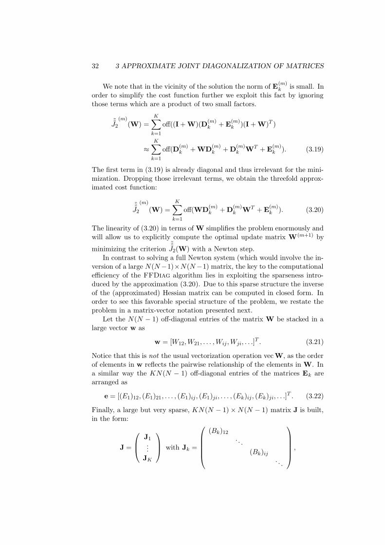
In contrast to solving a full Newton system (which would involve the in-version of a large N(N−1)×N(N−1) matrix, the key to the computationalefficiency of the FFDiag algorithm lies in exploiting the sparseness intro-duced by the approximation (3.20). Due to this sparse structure the inverseof the (approximated) Hessian matrix can be computed in closed form. Inorder to see this favorable special structure of the problem, we restate theproblem in a matrix-vector notation presented next.
Let the N(N − 1) off-diagonal entries of the matrix W be stacked in alarge vector w as
w = [W12,W21, . . . ,Wij ,Wji, . . .]T . (3.21)
Notice that this is not the usual vectorization operation vec W, as the orderof elements in w reflects the pairwise relationship of the elements in W. Ina similar way the KN(N − 1) off-diagonal entries of the matrices Ek arearranged as
e = [(E1)12, (E1)21, . . . , (E1)ij , (E1)ji, . . . , (Ek)ij , (Ek)ji, . . .]T . (3.22)
Finally, a large but very sparse, KN(N − 1)×N(N − 1) matrix J is built,in the form:
J =
J1...
JK
with Jk =
(Bk)12. . .
(Bk)ij. . .
,

3.3 COMPUTATION OF THE UPDATE MATRIX 33
where each Jk is block-diagonal, containing N(N − 1)/2 matrices of dimen-sion 2× 2
(Bk)ij =
((Dk)jj (Dk)ii(Dk)jj (Dk)ii
)
, i, j = 1, . . . , N, i 6= j,
where (Dk)ii is the (i, i)-th entry of a diagonal matrix Dk.Using this notation the threefold approximated cost function can be re-
written in the familiar form of a linear least-squares problem (Press et al.,1992).
˜J2(W) = (Jw + e)T (Jw + e). (3.23)
The vector w that minimizes (3.23) can be obtained in closed form as:
w = −(JTJ)−1JT e. (3.24)
We can now make use of the sparseness of J to enable the direct computationof the elements of w in (3.24). Writing out the matrix product JT J yieldsa block-diagonal matrix
JTJ =
∑
k((Bk)12)T (Bk)12
. . .∑
k(Bk)ij)T (Bk)ij
. . .
whose blocks are 2× 2 matrices. Thus the system (3.24) actually consists ofdecoupled equations
(Wij
Wji
)
= −(
zjj zij
zij zii
)−1(yij
yji
)
, i, j = 1, . . . , N, i 6= j, (3.25)
wherezij =
∑
k
(Dk)ii(Dk)jj
yij =∑
k
(Dk)jj(Ek)ij + (Ek)ji
2=∑
k
(Dk)jj(Ek)ij .
The matrix inverse in equation (3.25) can be computed in closed form, lead-ing us to the following expressions for the update of the entries of W:
Wij =zijyji − ziiyij
zjjzii − z2ij
,
Wji =zijyij − zjjyji
zjjzii − z2ij
.(3.26)
Here, only the off-diagonal elements (i 6= j) need to be computed and thediagonal terms of W are set to zero.
34 3 APPROXIMATE JOINT DIAGONALIZATION OF MATRICES
In the orthogonal case, due to the skew-symmetry of W, only one ofeach pair of the entries (3.26) needs to be computed since the other entry isset to Wji = −Wij. This yields the simpler expression for the elements ofW:
Wij =
∑
k(Ek)ij ((Dk)ii − (Dk)jj)∑
k((Dk)ii − (Dk)jj)2, i, j = 1, . . . , N, i 6= j, (3.27)
and reduces the computational cost by a factor of two.
Discussion
The simplifying assumptions used in (3.19) require some further discussion.Our motivation for assuming that W and Ek are small is based on theobservation that in the neighborhood of the solution, the matrices Ck arealmost diagonal and thus the steps W towards the optimum are small.
Hence, in the neighborhood of the optimal solution the algorithm is ex-pected to behave similarly to Newton’s method and can converge quadrati-cally.
We note however, that the assumption of small Ek is potentially prob-lematic, especially in the case where exact diagonalization is impossible. Inthis case it is preferable to carried out the gradient descent step in equation(3.18), where Ek is fully taken into account.
In any case the assumption of W being small is crucial for the conver-gence of the algorithm and needs to be carefully controlled. The latter isdone by the normalization (3.12).
Some general remarks on convergence properties of the proposed algo-rithmic scheme are due at this point. Newton-like algorithms are known toconverge only in the neighborhood of the optimal solution; however, whenthey converge, the rate of convergence is quadratic (e.g. Kantorovich, 1949).Since the essential components of our algorithm—the second-order approx-imation of the objective function and the computation of optimal steps bysolving the linear system arising from first-order optimality conditions—areinherited from Newton’s method, the same convergence behavior can beexpected.
The Newton direction in FFDiag is computed based on the Hessian ofthe threefold approximated cost function.2 Taking advantage of the resultingspecial structure, this computation can be carried out very efficiently:
Instead of performing inversion and multiplication of large matrices,which would have brought us to the same O(KN 6) complexity as in thealgorithm of van der Veen (2001), computation of the optimal W(m+1) leadsto a simple formula (3.26) which has to be evaluated for all N(N−1) entriesof W. Since the computation of zij and yij also involves a loop over K, theoverall complexity of the update step is O(KN 2).
2Furthermore, the Hessian is approximated by the product of the Jacobian matrices.

3.4 SUMMARY 35
3.4 Summary
We proposed new algorithms for simultaneous diagonalization of a set ofsymmetric matrices using multiplicative updates based on the matrix expo-nential as a structural constraint to prevent trivial solutions.
The close relations between the blind source separation problem andthe approximate joint diagonalization problem led us to specially adaptedparameterizations and approximations of a nonlinear least-squares cost func-tion.
The efficiency of the derived algorithm comes from the special second-order approximation of the cost function, which yields a block-diagonal Hes-sian and thus allows for highly efficient computation of a (quasi-) Newtonupdate step. The main result is a closed form solution for the update of apair of matrix elements.
The multiplicative update has the advantage of preserving the groupstructure of the problem.
For simplicity of the derivations we considered the case that the targetmatrices Ck are all real-valued and symmetric. An extension to the moregeneral, complex-valued case is possible, but has to be left for future work.

36 3 APPROXIMATE JOINT DIAGONALIZATION OF MATRICES

Chapter 4
Numerical Simulations
In the following, a series of numerical experiments aimedat comparing the performance of the algorithms on syntheticapproximate joint diagonalization tasks is provided.
4.1 Introduction
The experiments in this chapter are intended to demonstrate the perfor-mance of the newly developed AJD algorithms in general and in particularto compare the FFDiag algorithm with other state-of-the-art algorithmsfor approximate joint diagonalization of synthetic benchmark data and oftypical target matrices occurring in BSS applications.
To facilitate a comparison, we first introduce suitable measures of per-formance. Then we present the results of five progressively more complexexperiments. As a starting point we perform a “sanity check” experiment,i.e. to diagonalize a set of perfectly diagonalizable matrices which is a rela-tively easy task. This experiment is intended to emphasize that for small-size diagonalizable matrices the algorithm’s performance matches the ex-pected quadratic convergence. In the second experiment we compare theFFDiag algorithm with the extended Jacobi method as used in the JADEalgorithm of Cardoso and Souloumiac (1993) (orthogonal Frobenius normformulation), Pham’s algorithm for positive-definite matrices (Pham, 2001)and Yeredor’s AC-DC algorithm (Yeredor, 2002) (non-orthogonal, subspacefitting formulation). In the third experiment we investigate the scaling be-havior of our algorithm as compared to AC-DC. Furthermore, the perfor-mance of the FFDiag algorithm is tested and compared with the AC-DCalgorithm on noisy, non-diagonalizable matrices. Finally, the application ofour algorithm to BSS is illustrated.
37

38 4 NUMERICAL SIMULATIONS
4.2 Performance Measures
Evaluating the algorithms for approximate joint diagonalization requiresdefinite performance measures. The most straightforward measure of per-formance is to monitor the evolution of the objective function.
In synthetic experiments with artificial data the distance from the truesolution is a good evaluation criterion. To be meaningful, this distancehas to be invariant w.r.t. the irrelevant scaling and permutation ambigui-ties. For this reason, we choose a performance index that is commonly usedin the context of ICA/BSS where the same invariances exist (see e.g. inAmari and Cichocki, 1998; Cardoso, 1999). Following the formulation ofMoreau (2001) a suitable performance index is defined on the normalized
“global” matrix Mdef= VA according to
score(M) =1
2
∑
i
∑
j
|Mij |2max
l|Mil|2
− 1
+∑
j
∑
i
|Mij |2max
l|Mlj |2
− 1
.(4.1)
The first sum is small when each column of M has exactly one dominatingelement. The second sum gets small when each row of M has exactly onedominating element. The non-negative index (4.1) becomes zero iff M isa product of an invertible diagonal matrix D and of a permutation matrixP, i.e., M = DP. Thus, if the algorithm was successful, score(M = VA)should be close to zero.
4.3 FFDiag in Practice
4.3.1 “Sanity check” Experiment
The test data in this experiment is generated as follows. We use K = 15 di-agonal matrices Dk of size 5×5 where the elements on the diagonal are drawnfrom a uniform distribution in the range [−1, . . . , 1] (cf. Joho and Rahbar,2002). These matrices are ‘mixed’ by an orthogonal matrix A according toADkA
T to generate the set of target matrices {Ck} to be diagonalized.1
The FFDiag algorithm is initialized with the identity matrix V(0) = I, andthe skew-symmetric update rule (3.27) is used.
The convergence behavior of the algorithm in 10 runs is shown in Figure4.1. The diagonalization error is measured by the off(·) function. One cansee that the algorithm has converged to the correct solution after less than10 iterations in all trials. A quadratic convergence rate is observed fromearly iterations.
1 The orthogonal matrix was obtained from a singular value decomposition of a random5 × 5 matrix, where the entries are drawn from a standard normal distribution.
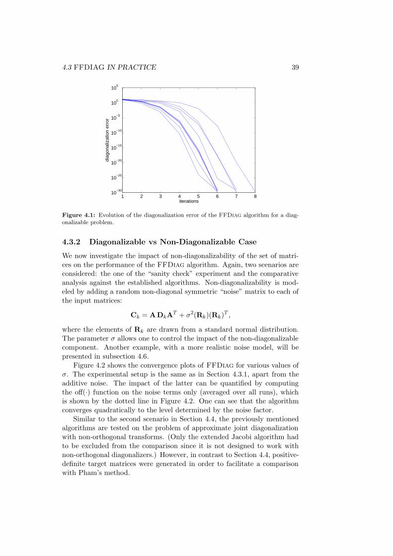
4.3 FFDIAG IN PRACTICE 39
1 2 3 4 5 6 7 810
−30
10−25
10−20
10−15
10−10
10−5
100
105
iterations
diag
onal
izat
ion
erro
r
Figure 4.1: Evolution of the diagonalization error of the FFDiag algorithm for a diag-onalizable problem.
4.3.2 Diagonalizable vs Non-Diagonalizable Case
We now investigate the impact of non-diagonalizability of the set of matri-ces on the performance of the FFDiag algorithm. Again, two scenarios areconsidered: the one of the “sanity check” experiment and the comparativeanalysis against the established algorithms. Non-diagonalizability is mod-eled by adding a random non-diagonal symmetric “noise” matrix to each ofthe input matrices:
Ck = ADkAT + σ2(Rk)(Rk)
T ,
where the elements of Rk are drawn from a standard normal distribution.The parameter σ allows one to control the impact of the non-diagonalizablecomponent. Another example, with a more realistic noise model, will bepresented in subsection 4.6.
Figure 4.2 shows the convergence plots of FFDiag for various values ofσ. The experimental setup is the same as in Section 4.3.1, apart from theadditive noise. The impact of the latter can be quantified by computingthe off(·) function on the noise terms only (averaged over all runs), whichis shown by the dotted line in Figure 4.2. One can see that the algorithmconverges quadratically to the level determined by the noise factor.
Similar to the second scenario in Section 4.4, the previously mentionedalgorithms are tested on the problem of approximate joint diagonalizationwith non-orthogonal transforms. (Only the extended Jacobi algorithm hadto be excluded from the comparison since it is not designed to work withnon-orthogonal diagonalizers.) However, in contrast to Section 4.4, positive-definite target matrices were generated in order to facilitate a comparisonwith Pham’s method.
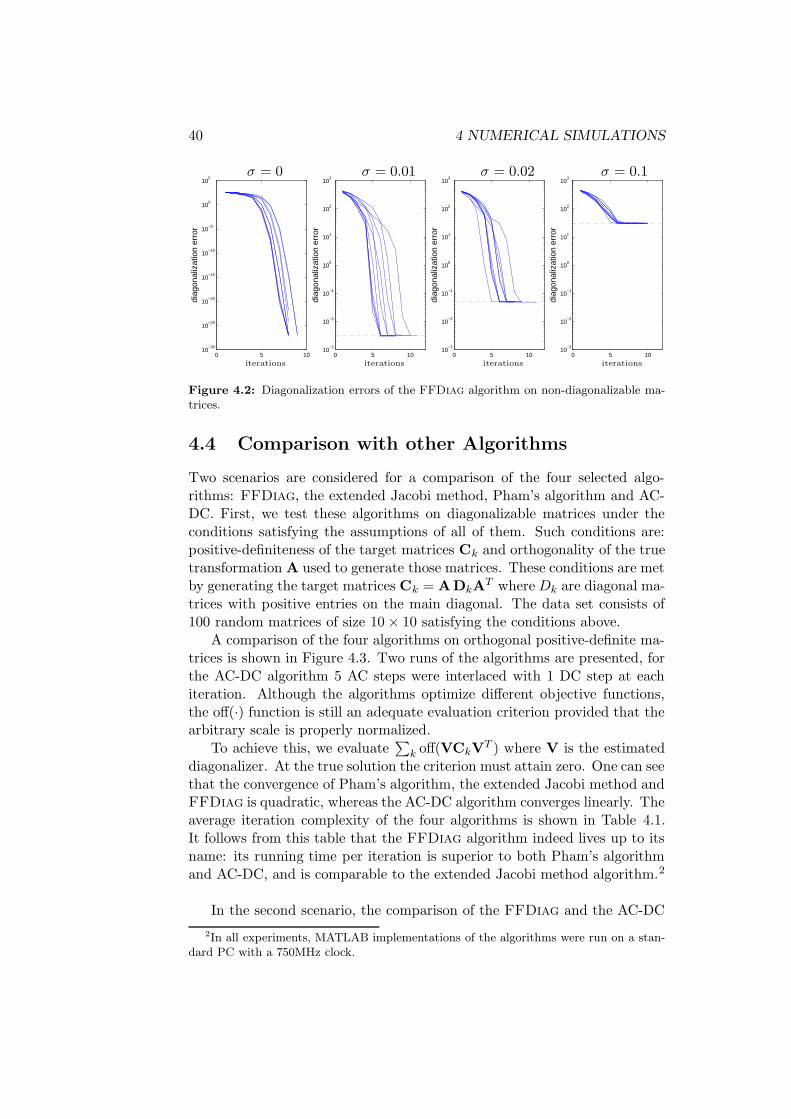
40 4 NUMERICAL SIMULATIONS
0 5 1010
−30
10−25
10−20
10−15
10−10
10−5
100
105
diag
onal
izat
ion
erro
r
0 5 1010
−3
10−2
10−1
100
101
102
103
diag
onal
izat
ion
erro
r
0 5 1010
−3
10−2
10−1
100
101
102
103
diag
onal
izat
ion
erro
r
0 5 1010
−3
10−2
10−1
100
101
102
103
diag
onal
izat
ion
erro
r
PSfrag replacements
iterationsiterationsiterationsiterations
σσσσ = 0 = 0.1= 0.01 = 0.02
Figure 4.2: Diagonalization errors of the FFDiag algorithm on non-diagonalizable ma-trices.
4.4 Comparison with other Algorithms
Two scenarios are considered for a comparison of the four selected algo-rithms: FFDiag, the extended Jacobi method, Pham’s algorithm and AC-DC. First, we test these algorithms on diagonalizable matrices under theconditions satisfying the assumptions of all of them. Such conditions are:positive-definiteness of the target matrices Ck and orthogonality of the truetransformation A used to generate those matrices. These conditions are metby generating the target matrices Ck = ADkA
T where Dk are diagonal ma-trices with positive entries on the main diagonal. The data set consists of100 random matrices of size 10× 10 satisfying the conditions above.
A comparison of the four algorithms on orthogonal positive-definite ma-trices is shown in Figure 4.3. Two runs of the algorithms are presented, forthe AC-DC algorithm 5 AC steps were interlaced with 1 DC step at eachiteration. Although the algorithms optimize different objective functions,the off(·) function is still an adequate evaluation criterion provided that thearbitrary scale is properly normalized.
To achieve this, we evaluate∑
k off(VCkVT ) where V is the estimated
diagonalizer. At the true solution the criterion must attain zero. One can seethat the convergence of Pham’s algorithm, the extended Jacobi method andFFDiag is quadratic, whereas the AC-DC algorithm converges linearly. Theaverage iteration complexity of the four algorithms is shown in Table 4.1.It follows from this table that the FFDiag algorithm indeed lives up to itsname: its running time per iteration is superior to both Pham’s algorithmand AC-DC, and is comparable to the extended Jacobi method algorithm.2
In the second scenario, the comparison of the FFDiag and the AC-DC
2In all experiments, MATLAB implementations of the algorithms were run on a stan-dard PC with a 750MHz clock.

4.4 COMPARISON WITH OTHER ALGORITHMS 41
2 4 6 8 10 12 14
10−25
10−20
10−15
10−10
10−5
100
iterations
diag
onal
izat
ion
erro
rorth. FFDIAGext. JacobiPham’sAC−DC
Figure 4.3: Comparison of the FFDiag, the extended Jacobi method, Pham’s algorithmand AC-DC in the orthogonal, positive-definite case: diagonalization error per iterationmeasured by the off(·) criterion.
FFDiag ext. Jacobi Pham’s AC-DC
0.025 0.030 0.168 2.430
Table 4.1: Comparison of the FFDiag, ext. Jacobi, Pham’s and AC-DC algorithms inthe orthogonal, positive-definite case: average running time per iteration in seconds.
algorithms is repeated for non-positive-definite matrices obtained from anon-orthogonal mixing matrix. This case cannot be handled by the othertwo algorithms, therefore they are omitted from the comparison. The con-vergence plots are shown in Figure 4.4; average running time per iterationis reported in Table 4.2. Convergence behavior of the two algorithms is thesame as in the orthogonal, positive-definite case; the running time per iter-ation of FFDiag increases due to the use of non-skew-symmetric updates.
FFDiag AC-DC
0.034 2.64
Table 4.2: Comparison of the FFDiag and AC-DC algorithms in the non-orthogonal,non-positive-definite case: average running time per iteration in seconds.
The results of the comparison of the FFDiag, Pham’s and AC-DC algo-rithms on a non-orthogonal positive-definite problem (5 matrices of dimen-
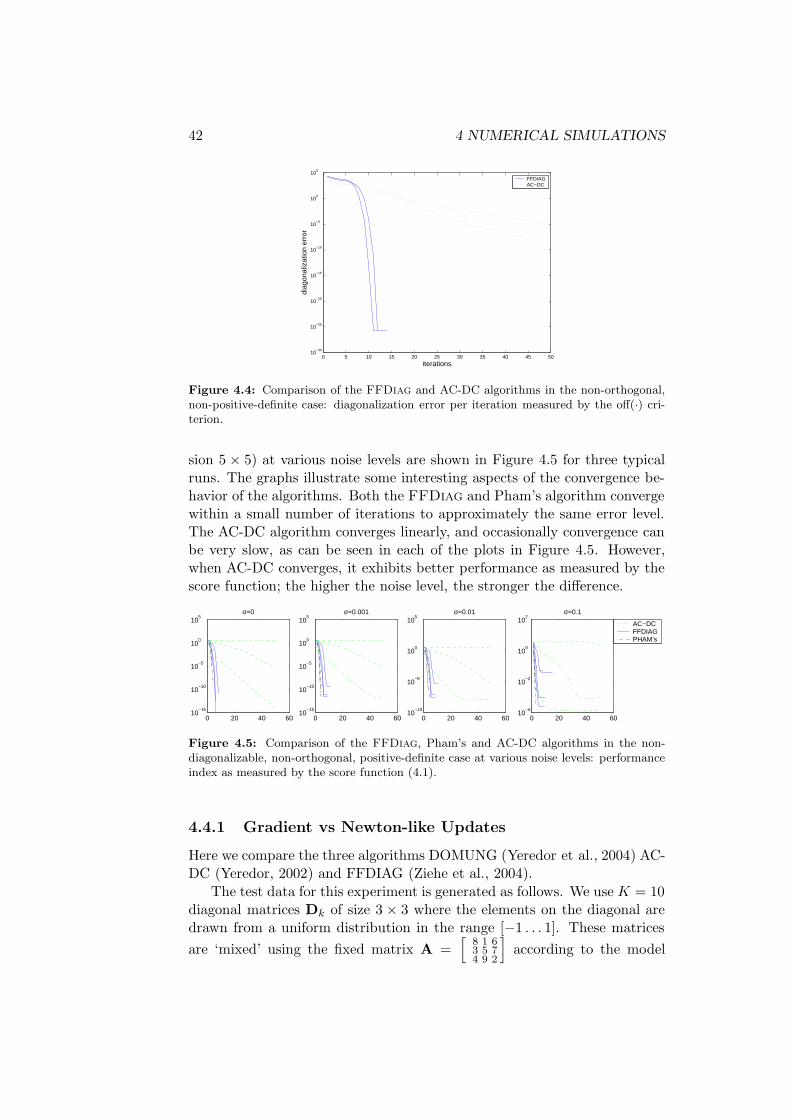
42 4 NUMERICAL SIMULATIONS
0 5 10 15 20 25 30 35 40 45 5010
−30
10−25
10−20
10−15
10−10
10−5
100
105
iterations
diag
onal
izat
ion
erro
r
FFDIAGAC−DC
Figure 4.4: Comparison of the FFDiag and AC-DC algorithms in the non-orthogonal,non-positive-definite case: diagonalization error per iteration measured by the off(·) cri-terion.
sion 5 × 5) at various noise levels are shown in Figure 4.5 for three typicalruns. The graphs illustrate some interesting aspects of the convergence be-havior of the algorithms. Both the FFDiag and Pham’s algorithm convergewithin a small number of iterations to approximately the same error level.The AC-DC algorithm converges linearly, and occasionally convergence canbe very slow, as can be seen in each of the plots in Figure 4.5. However,when AC-DC converges, it exhibits better performance as measured by thescore function; the higher the noise level, the stronger the difference.
0 20 40 6010
−15
10−10
10−5
100
105
σ=0
0 20 40 6010
−15
10−10
10−5
100
105
σ=0.001
0 20 40 6010
−10
10−5
100
105
σ=0.01
0 20 40 6010
−4
10−2
100
102
σ=0.1
AC−DCFFDIAGPHAM’s
Figure 4.5: Comparison of the FFDiag, Pham’s and AC-DC algorithms in the non-diagonalizable, non-orthogonal, positive-definite case at various noise levels: performanceindex as measured by the score function (4.1).
4.4.1 Gradient vs Newton-like Updates
Here we compare the three algorithms DOMUNG (Yeredor et al., 2004) AC-DC (Yeredor, 2002) and FFDIAG (Ziehe et al., 2004).
The test data for this experiment is generated as follows. We use K = 10diagonal matrices Dk of size 3 × 3 where the elements on the diagonal aredrawn from a uniform distribution in the range [−1 . . . 1]. These matrices
are ‘mixed’ using the fixed matrix A =[
8 1 63 5 74 9 2
]
according to the model
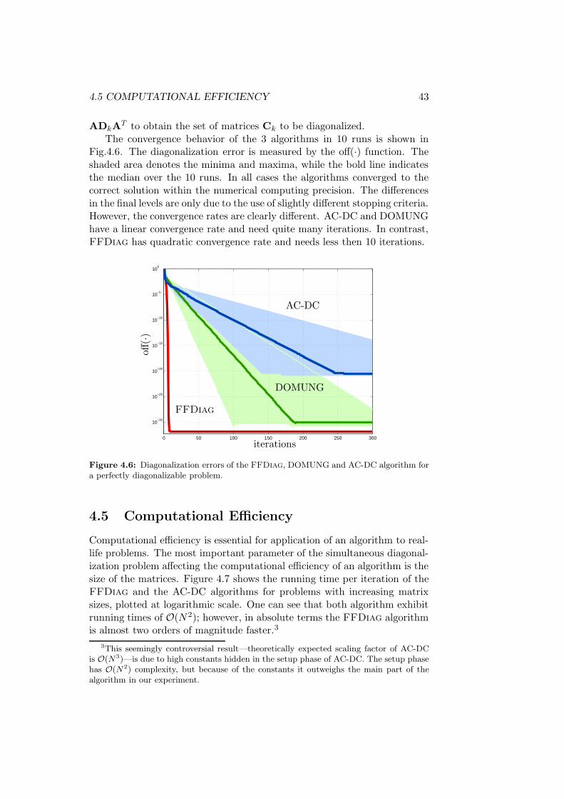
4.5 COMPUTATIONAL EFFICIENCY 43
ADkAT to obtain the set of matrices Ck to be diagonalized.
The convergence behavior of the 3 algorithms in 10 runs is shown inFig.4.6. The diagonalization error is measured by the off(·) function. Theshaded area denotes the minima and maxima, while the bold line indicatesthe median over the 10 runs. In all cases the algorithms converged to thecorrect solution within the numerical computing precision. The differencesin the final levels are only due to the use of slightly different stopping criteria.However, the convergence rates are clearly different. AC-DC and DOMUNGhave a linear convergence rate and need quite many iterations. In contrast,FFDiag has quadratic convergence rate and needs less then 10 iterations.
0 50 100 150 200 250 300
10−30
10−25
10−20
10−15
10−10
10−5
100
PSfrag replacements
FFDiag
AC-DC
DOMUNG
iterations
off(·)
Figure 4.6: Diagonalization errors of the FFDiag, DOMUNG and AC-DC algorithm fora perfectly diagonalizable problem.
4.5 Computational Efficiency
Computational efficiency is essential for application of an algorithm to real-life problems. The most important parameter of the simultaneous diagonal-ization problem affecting the computational efficiency of an algorithm is thesize of the matrices. Figure 4.7 shows the running time per iteration of theFFDiag and the AC-DC algorithms for problems with increasing matrixsizes, plotted at logarithmic scale. One can see that both algorithm exhibitrunning times of O(N 2); however, in absolute terms the FFDiag algorithmis almost two orders of magnitude faster.3
3This seemingly controversial result—theoretically expected scaling factor of AC-DCis O(N3)—is due to high constants hidden in the setup phase of AC-DC. The setup phasehas O(N2) complexity, but because of the constants it outweighs the main part of thealgorithm in our experiment.

44 4 NUMERICAL SIMULATIONS
0 10 20 30 40 5010
−3
10−2
10−1
100
101
102
dimension of matrices
time
per
itera
tion
in s
econ
ds
FFDIAGAC−DC
Figure 4.7: Scaling of the FFDiag and AC-DC algorithms with respect to the matrixsize. Two repetitions of the experiment have been performed.
4.6 Blind Source Separation
4.6.1 Blind Separation of Audio Signals
We apply the joint diagonalization algorithms to a blind source separationtask. Here the source signal matrix S contains seven audio signals containing10000 points recorded at 8kHz and one Gaussian noise source of the samelength (see Fig. 4.9). These signals are mixed by a 8× 8 Hadamard matrix,
A =
1 1 1 1 1 1 1 11 −1 1 −1 1 −1 1 −11 1 −1 −1 1 1 −1 −11 −1 −1 1 1 −1 −1 11 1 1 1 −1 −1 −1 −11 −1 1 −1 −1 1 −1 11 1 −1 −1 −1 −1 1 11 −1 −1 1 −1 1 1 −1
.
This scaled orthogonal matrix produces a complete mixture X = AS (seeFig. 4.9, middle panel), in the sense that each observation contains a maxi-mal contribution from each source.
In order to separate these signals, we compute 100 symmetrized, time-lagged correlation matrices according to Equation (2.12) and then apply theFFDiag algorithm with V(0) = I. Figure 4.8 shows the evolution of thenormalized diagonalization error. One can see that the algorithm convergedafter 6 iterations and that the normalized global system V(m)A converges toa permutation matrix (as shown in the left and the right panels of Fig. 4.8,respectively). The good performance can also be seen from Figure 4.9,where we observe a good match between the separated signals U and thetrue source signals S.

4.6 BLIND SOURCE SEPARATION 45
0 2 4 6 8 1010
−2
10−1
100
iterations
norm
aliz
ed d
iago
naliz
atio
n er
ror
channel #
chan
nel #
1 2 3 4 5 6 7 8
1
2
3
4
5
6
7
8
Figure 4.8: Convergence progress of the AJD4BSS algorithm on the BSS task. The right
panel shows the entries of the matrix V(m)A for the final (10th) iteration and indicatessuccessful separation, since the cross-talk is minimized and V(10)A resembles a scaled andpermuted identity matrix. Here, black and white squares correspond to values 1 and 0,respectively.
4.6.2 Noisy mixtures
In order to study the behavior of the FFDiag algorithm in a more realisticnoisy scenario the following experiment is conducted.
Input data is generated by mixing three stationary, time-correlated sources
with the fixed matrix A =(
8 1 63 5 74 9 2
)
. The sources are generated by feeding
an i.i.d. random noise signal into a randomly chosen, auto-regressive (AR)model of order 5 whose coefficients are drawn from a standard normal dis-tribution and are sorted in decreasing order (to ensure stability). The gen-erated signals have a total length of 50000 samples. To separate the sourceswe estimate 10 symmetrized, time-lagged correlation matrices of the mixedsignals according to Equation (2.12) and perform simultaneous diagonal-ization of these matrices. The number T of samples used to estimate thecorrelation matrices determines the quality of the estimates. Thus, by vary-ing T , we simulate different noise levels corresponding to different variancesof the estimate. This procedure is more realistic than simply corrupting thetarget matrices with small additive i.i.d. noise.
The results of the experiment are shown in Figure 4.10. The perfor-mance of the FFDiag and the AC-DC algorithm, as measured by the score(4.1), is displayed for four different sample sizes, where small samples sizescorrespond to a higher noise level. 100 repetitions are performed for eachsample size, and the 25%, 50% and 75% quantiles of the log-score are shownin the plots. Two observations can be made from Figure 4.10: FFDiag
converges much faster than AC-DC, and when converged, FFDiag yields abetter score (on average), with the difference more pronounced for samplessizes 10000 and 30000 in our experiment.
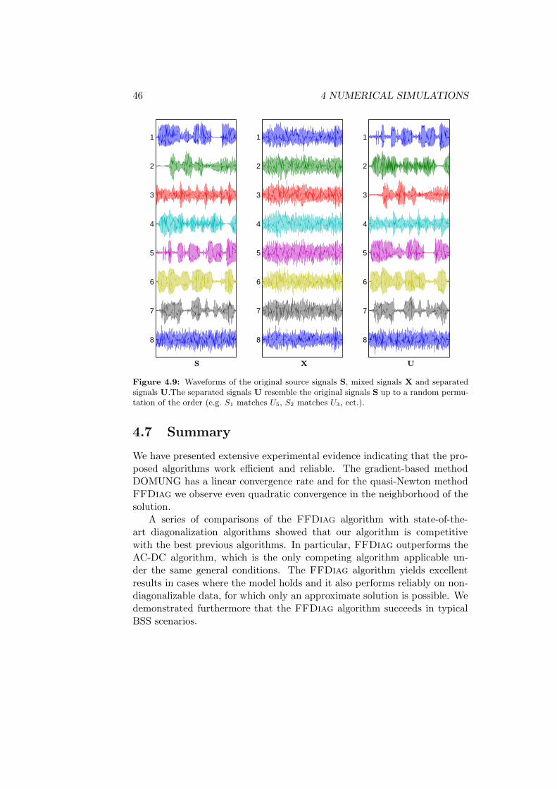
46 4 NUMERICAL SIMULATIONS
1
2
3
4
5
6
7
8
1
2
3
4
5
6
7
8
1
2
3
4
5
6
7
8
PSfrag replacements
S X U
Figure 4.9: Waveforms of the original source signals S, mixed signals X and separatedsignals U.The separated signals U resemble the original signals S up to a random permu-tation of the order (e.g. S1 matches U5, S2 matches U3, ect.).
4.7 Summary
We have presented extensive experimental evidence indicating that the pro-posed algorithms work efficient and reliable. The gradient-based methodDOMUNG has a linear convergence rate and for the quasi-Newton methodFFDiag we observe even quadratic convergence in the neighborhood of thesolution.
A series of comparisons of the FFDiag algorithm with state-of-the-art diagonalization algorithms showed that our algorithm is competitivewith the best previous algorithms. In particular, FFDiag outperforms theAC-DC algorithm, which is the only competing algorithm applicable un-der the same general conditions. The FFDiag algorithm yields excellentresults in cases where the model holds and it also performs reliably on non-diagonalizable data, for which only an approximate solution is possible. Wedemonstrated furthermore that the FFDiag algorithm succeeds in typicalBSS scenarios.
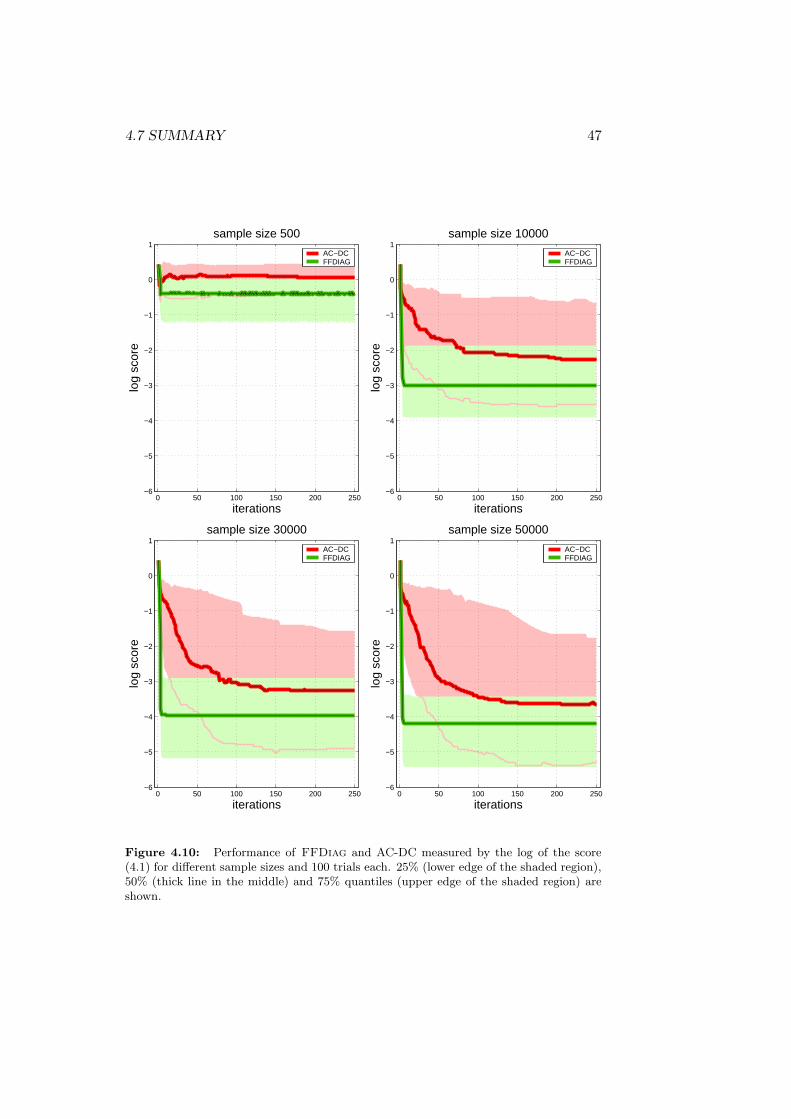
4.7 SUMMARY 47
0 50 100 150 200 250−6
−5
−4
−3
−2
−1
0
1
iterations
log
scor
e
sample size 500
AC−DCFFDIAG
0 50 100 150 200 250−6
−5
−4
−3
−2
−1
0
1
iterations
log
scor
e
sample size 10000
AC−DCFFDIAG
0 50 100 150 200 250−6
−5
−4
−3
−2
−1
0
1
iterations
log
scor
e
sample size 30000
AC−DCFFDIAG
0 50 100 150 200 250−6
−5
−4
−3
−2
−1
0
1
iterations
log
scor
e
sample size 50000
AC−DCFFDIAG
Figure 4.10: Performance of FFDiag and AC-DC measured by the log of the score(4.1) for different sample sizes and 100 trials each. 25% (lower edge of the shaded region),50% (thick line in the middle) and 75% quantiles (upper edge of the shaded region) areshown.

48 4 NUMERICAL SIMULATIONS

Chapter 5
Applications
This chapter describes applications of blind source separa-tion methods in biomedical signal processing. We demon-strate the usefulness of the proposed approach in the analysisof real-world neuro-physiological signals. The focus lies onusing the joint diagonalization techniques in different sce-narios where appropriate target matrices derived from themulti-channel measurements can be approximately diagonal-ized. The material presented in this chapter is partially basedon the publications Ziehe et al. (2001) and Vigario et al.(2002); Wubbeler et al. (2000).
In the following we will present applications involving only the linearinstantaneous BSS problem according to Equation (2.1). Even though thismodel is rather simple, it is particularly useful for biomedical signal process-ing as will be shown in the next section.
5.1 Biomedical signal processing
An example of BSS application for real-world biomedical signal processing isthe analysis and pre-processing of electroencephalographic (EEG) and mag-netoencephalographic (MEG) measurements. Here the routine usage of largesensor arrays (some of them consist of up to 300 SQUID-magnetometers)to record neuromagnetic fields in humans, produces data that suits theBSS approach quite well. Due to the fact that the electromagnetic wavessuperimpose linearly and virtually instantaneously (because of the rela-tively small distance from sources to sensors) the instantaneous linear model(5.1) is valid (Makeig et al., 1996; Vigario et al., 1998; Vigario et al., 2000;Wubbeler et al., 2000; Ziehe et al., 2000a).
x(t) = As(t), (5.1)
49

50 5 APPLICATIONS
The columns of A represent the coupling of a source with each sensor.Since the array geometry is known, this information gives rise to a spatialfield pattern. The the sources s(t) display the time courses of the compo-nents. It is precisely this decoupling of spatial and temporal informationthat makes these decompositions a valuable tool for exploratory data anal-ysis.
The difficulties in the application those (blind) decompositions —as forany unsupervised data analysis—lie in the correctness and validation of theused modeling assumptions. Although our proposed methods are based onrelatively “mild” assumptions they must still be verified for the particularapplication. In other words, it should always be checked whether or not theassumptions are fulfilled. In cases where this is not fully possible, one canstill apply the method but one should be aware that a critical evaluation ofthe results —preferably based on medical knowledge— is needed.
Some of the limitations of the presented BSS-based approaches are thefollowing:
These methods can extract at most as many underlying sources as thenumber of sensors. For example, in MEG and EEG analysis, a multitude ofmicroscopic brain sources is present, which outnumbers by far the numberof sensors used to record the magnetic or electric fields. Nevertheless, itcan be argued that the total number of macroscopically observable sources,active at a given time-interval, is sufficiently smaller, and thus the use ofICA/BSS methods can be justified.
The use of separation criteria based on high-order statistics (e.g. in theJADE algorithm or kurtosis-based FastICA variants) comes at a price: anincreased sensitivity to outliers. These often turn out to be the dominatingfactors in the decomposition due to their extreme non-Gaussianity.
Another issue that has to be kept in mind when applying higher-orderstatistics methods to large-scale sensor array data is the high computationalload. For example in JADE the effort for storing and processing the 4-thorder cumulants is O(N 4), where N is the number of sensors. Since this maybe prohibitively large, the data has to be projected to a lower dimensionalsubspace as a preprocessing step.
For this reason we advocate methods which rely on second-order statis-tics only and additionally make use of the time-structure of the data. Thediagonalization based procedures if employed on ensembles of suitable cor-relation matrices are expected to be superior in those respects.
5.1.1 Artifact Reduction by Adaptive Spatial Filtering
In the analysis of EEG and MEG data one often faces the problem that noisefrom biological or technical origins (like alpha rhythm activity or interferencefrom power-lines, respectively) is corrupting the measurements.
In this section we study the capabilities of blind source separation to
5.1 BIOMEDICAL SIGNAL PROCESSING 51
construct an adaptive spatial filter that isolates the power-line signal whilepreserving evoked responses. We compare the spatial filtering by BSS to aclassical notch filtering.
These frequency domain filtering techniques can also be applied to sup-press power-line artifacts, this standard approach is clearly limited to nar-row band signals. In contrast, BSS based spatial filtering methods are notrelying on known narrow-band spectral characteristics but rather look forindependent or temporally uncorrelated source signals (Vigario et al., 1998;Ziehe et al., 2000a).
Data
In this case study we analyze the effects of artifact removal in a typicalexperimental setting. The specific data set studied is obtained from mea-surements of somatosensory evoked fields (SEF, N20) and provides an at-tractive and rather controlled testbed since the signal of interest (N20) isrelatively strong and the origin of the generator in the post-central gyrus iswell-known.
Signals were measured using a low noise 63-channel DC-SQUID system(white noise level 2.7fT/
√Hz) operated in a first order axial electronic gra-
diometer mode with 70mm baseline; 7mm diameter SQUID pick up area, 49sensors in a planar hexagonal configuration for the registration of the verti-cal field component, 30 mm distance between neighboring SQUID positionscovering an area of 210 mm diameter (Drung, 1995).
The right median nerve was stimulated over 12.000 epochs, while the themagnetic field above the left somatic sensory cortex was measured using 49planar gradiometer sensors. A sampling rate of 2 kHz and an inter-stimulusinterval (ISI) of 333 msec were used to avoid steady state effects.
The recordings were carried out by the PTB1 at the biomagnetism lab-oratory in the Department of Neurology at the campus Benjamin Franklinof the Charite2.
Although sophisticated magnetic shielding is used, a contamination ofthe measured biosignals by power-line interference can often not be com-pletely avoided.
Artifact Reduction Procedure
The BSS based artifact reduction procedure consists of the following steps:
• apply a sphering and dimensionality reduction (based on PCA).
• decompose the transformed data into independent components by aBSS algorithm.
1The Physikalisch-Technische Bundesanstalt of Germany.2 The Charite - University Medicine Berlin.

52 5 APPLICATIONS
50 100 150 200 250 300
�150
�100
�50
0
50
100
150
time (ms)
B (
fT)
N20
Figure 5.1: SEF averaged data of all 49 channels
• decide which components correspond to artifactual or relevant signals(e.g. by using prior medical knowledge).
• project the previously selected components of interest back to sensorspace.
Applying this procedure we obtain a set of cleaned measurements.
Another possibility is to remove the artifact fields by making use of theirestimated spatial structure (contained in the columns of the mixing matrixA) by Signal-Space Projection (SSP) (Uusitalo and Ilmoniemi, 1997). Incase of multiple artifacts the whole space spanned by these artifacts, whichwe will refer to as “artifact space”, has to be projected out. The corre-sponding projector is conveniently written in terms of an orthonormal basisof the artifact space. The essential requirement for applying SSP is that theunwanted fields are known up to unknown multiplicative constants which isexactly the case for the BSS model.
Performance Evaluation
The results of the BSS based procedure are compared to notch filtering (witha properly tuned notch frequency) as a “gold standard”. A further indicationof the success of the method can be gained by looking at the reduction ofthe peak at 150 Hz in the power spectrum Also the “goodness-of-fit” of anequivalent current dipole (ECD) model may provide a validation criteria, atleast if based on a realistic volume conductor model.

5.1 BIOMEDICAL SIGNAL PROCESSING 53
Results
Predominantly two components with 150 Hz power were identified in thedecomposition (Fig. 5.2) when using BSS.
0 200 400 600 800 1000−50
0
50
Frequency
mag
nitu
de(d
B)
0 50 100 150 200 250 300 350−2
0
2
0 200 400 600 800 1000−50
0
50
Frequency
mag
nitu
de(d
B)
0 50 100 150 200 250 300 350−2
0
2
t (ms)
150 Hz
t (ms)
PSfrag replacements
(a)
(b)
Figure 5.2: Identified power-line signals.
Eliminating these artifacts we find that BSS based techniques yield sim-ilar results as the “gold standard” notch filtering approach in a data-drivenmanner, provided that the sample size was larger than 400 samples (seeFig. 5.3).
The goodness-of-fit of the dipole model was even better when using BSSmethods (cf. Fig. 5.4).

54 5 APPLICATIONS
200 250 300 350 400 450 500 550 600 6500
5
10
15
20
25
30
35
# samples
devi
atio
n in
%
TDSEPτ=0..5
JADE fastICA
gauss
fastICAtanh
Notch filter
Figure 5.3: Deviation of the normalized field at N20 from the “gold standard” forvarying sample size.
1 2 3 4 5 6 799
99.2
99.4
99.6
99.8
100
method
good
ness
−of
−fit
in %
TDSEP JADE
fastICAgauss
fastICAtanh
adaptive notch
fixed notch
original data
PSfrag replacements
Figure 5.4: Goodness of fit at N20 for various methods.

5.1 BIOMEDICAL SIGNAL PROCESSING 55
Figure 5.5: Source localization of N20 using the CURRY software with a realisticvolume-conductor model from an MRI scan.

56 5 APPLICATIONS
5.1.2 DC Magnetometry
In this section we report on the application of the joint diagonalization basedBSS methods to data reflecting ’direct current’ (DC-) activity in the humanbrain.
Since previously BSS techniques had been successfully applied to reduceartifacts in multi-channel EEG, MEG and MNG (magnetoneurography)recordings (Makeig et al., 1996; Vigario et al., 1998; Ziehe et al., 2000a) andto analyze evoked responses (Makeig et al., 1997) these methods were alsoexpected to provide interesting decompositions of neuromagnetic data evenin the near-DC range.
The identification of near-DC fields with non-invasive neuromagneticrecordings has great relevance for medical applications since slowly vary-ing DC-phenomena have been found e.g. in cerebral anoxia and spreadingdepression in (invasive) animal studies. Blind source separation techniqueshave a high potential to become a standard clinical procedure for analysingsuch data.
Medical Background
Recently, the feasibility of a non-invasive magnetic registration of near-DC(below 0.1 Hz) magnetic fields from the human cortex using SuperconductingQuantum Interference Devices (SQUIDs) has been shown (Mackert et al.,1999b). Such near-DC phenomena may have importance for metabolic in-juries of brain cells in stroke or migraine (Back et al., 1994; Chen et al.,1992; Gardner-Medwin et al., 1991). Being able to perform a DC-coupledbrain monitoring is of high medical relevance because many pathophysiolog-ical processes have their main energy in the frequency range below 0.1 Hz.Therefore, it is of great importance to further improve the signal extractionfrom DC-MEG data.
Technical background
The biomagnetic recording technology employed in this application is basedon a unique apparatus that mechanically moves the subjects head, respec-tively, body relative to the sensor array (Wubbeler et al., 1999).
This transposes the near-DC signals of the head/body to the modulationfrequency with lower 1/f noise. After signal demodulation this approach hasa dynamical sensitivity to detect DC-fields > 30 fT in a 100 sec evaluationperiod (Wubbeler et al., 1999). This yields a high sensitivity which is bothchance and challenge since it will not only enable physicians to detect minutephysiological fields (Curio et al., 1993; Mackert et al., 1999a) but also posesproblems for data analysis since the magnetic fields of a multitude of dif-ferent biological processes and noise superimpose the signal of interest. It

5.1 BIOMEDICAL SIGNAL PROCESSING 57
is a helpful matter of fact that many of these processes vary in intensityindependently of each other.
He Dewar He Dewar
PSfrag replacements
Fixed source Moving source
SQUIDs withHelium dewar
B(t)B(t)
magnetic sources
∆B
tt
Figure 5.6: Modulation principle for DC measurements. Characteristic magnetometeroutput for a fixed and a moving source. The sinusodial movement of the source beneaththe magnetometer array leads to an oscillating field signal.
Experimental Setup
In Mackert et al. (1999b) a paradigm of prolonged auditory (music) stim-ulation for DC-MEG was introduced. It consists of presenting 30 secondsof music and 30 seconds of silence to the subjects ear. This experimentalsetting has the advantages that a physiological DC-source in the brain withan essentially known field pattern3 can be switch “on” and “off” arbitrarilyby external non-invasive stimulation.
Data Acquisition and Validation
The neuromagnetic field data were recorded in a standard magneticallyshielded room (AK3b), operated at the “Benjamin Franklin” hospital bythe PTB, using 49 low noise first order SQUID gradiometers (70 mm base-line) covering a planar area of 210 mm diameter (Drung, 1995). The sensor
3The field patterns were expected to be comparable to patterns of evoked activities ofauditory cortices as reported in Pantev et al. (1996).

58 5 APPLICATIONS
was centered tangentially approximately over the left auditory cortex. Theacoustic stimulation was achieved by presenting alternating periods of musicand silence, each of 30 s length, to the subjects right ear during 30 min. oftotal recording time. The DC magnetic field values were acquired by usinga mechanical horizontal modulation of the body position with a frequencyof 0.4 Hz and an amplitude of 75 mm. This modulation transposed theDC magnetic field of the subject to the modulation frequency, which is lesscontaminated by magnetic noise (see also Fig. 5.6). The recorded magneticfield data were processed by digital lock-in techniques in order to extract themodulation induced frequency components (Wubbeler et al., 1998). Thenthe DC-field of the subject was reconstructed from these frequency compo-nents by using a transformation technique based on a virtual magnetic fieldgenerator (Mackert et al., 1999b). These reconstructed DC magnetic fieldvalues, sampled at the modulation frequency of 0.4 Hz, gave a total numberof 720 sample points per channel for the 30 minutes recording time and wereused as input for the BSS-algorithms.
Figure 5.7: Input data (after DC demodulation) arranged according to sensor positions.
Let us examine the time courses of 30 minutes for all 49 channels (cf. Fig. 5.7).At the first glance, the signals have an obvious trend behavior (slow drift)while possible components of interest are covered by other strong signals of

5.1 BIOMEDICAL SIGNAL PROCESSING 59
unknown origin, i.e. the response to the stimulus is completely hidden in thedata.
The above described experimental paradigm of externally controlledmusic-related DC-activations of auditory cortices defines a measurement andanalysis scenario with almost complete knowledge about both, the spatialpattern and the time course of a cerebral DC-source which on the other handis fully embedded in the biological and ambient noise background. Hence itmay serve as a testbed for a critical comparison of different BSS approachesfacing the ‘real world’ problems of bad signal-to-noise ratio coming alongwith a limited number of data samples and—on top of that—the presenceof outliers.
Matrices to be Diagonalized
First, the originally 49-dimensional sensor data were reduced by PCA andonly the 23 most powerful principal components were used.
When applying TDSEP (Ziehe and Muller, 1998) to the preprocesseddata, we compute time-lagged correlation matrices of the form
Cτ (x) = 〈x(t)xT (t− τ)〉 =
φx1,x1(τ) · · · φx1,xn(τ)φx2,x1(τ) · · · φx2,xn(τ)
.... . .
...φxn,x1(τ) · · · φxn,xn(τ)
where φxi,xj(τ) = 〈xi(t)xj(t− τ)〉 denote the respective auto– or cross–
correlation functions.Here 50 time-lagged correlation matrices (τ = 1..50 sample points) were
used for approximate joint diagonalization.
Results
The 10 strongest ICA components are shown in Fig. 5.9. Not surprisingly,one component (ICA1) mainly captured the slow drift, that was alreadyvisible in the data in Fig. 5.7. While most other components show irregulartime courses reflecting the dynamics of undetermined processes it is note-worthy that their field maps feature spatially coherent field patterns whichclearly distinguish them from random channel noise patterns.
Remarkably, one component (ICA10) shows a (noisy) rectangular wave-form. Its time course and frequency (see Fig. 5.8) clearly resembles the 1
30s
“on/off” characteristics of the stimulus. The spatial field distribution ofICA10 shows a bipolar pattern, located at the expected position of corti-cal activity (Mackert et al., 1999b). Both findings give direct evidence thatICA10 represents the response to the acoustical stimulus. Although wedo not expect that the cortical response resembles the stimulus completely,computing the correlation coefficient between the stimulus and the ICA time

60 5 APPLICATIONS
Figure 5.8: Spatial field pattern, frequency content and time course of ICA10.
courses provides a useful measure to evaluate and compare the performanceof different separation algorithms. Applying the three algorithms JADE(Cardoso and Souloumiac, 1993), FastICA (Hyvarinen and Oja, 1997) andTDSEP (Ziehe and Muller, 1998), we find that only the temporal decorre-lation algorithm TDSEP is able to recover a signal that is highly correlatedto the stimulus, while FastICA and JADE fail for this specific task (forcorrelation coefficients see also Fig. 5.10).
Conclusion
Based on a comparison of several approaches, we found out that methodsbased on spatio-temporal decorrelation are able to successfully extract acomponent related to a sustained DC activation in the auditory cortex whichwas induced by presentation of music. The task is especially challenging dueto the limited amount of available data and the occurrence of outliers. Sincesuch a situation is very typical for biomedical measurements, this datasetprovides also a useful real-world testbed for evaluating the performance androbustness of different BSS approaches.
It turned out that outliers can strongly decrease the performance of ICAalgorithms, in particular methods that use higher-order statistics explicitly(e.g. JADE, FastICA with kurtosis) fail for this dataset, while in contrastspatio-temporal decorrelation methods based on joint-diagonalization of sev-eral time-delayed correlation matrices proved to be more robust.
From a general physiological point of view it is interesting to note thatwhen employing these decomposition algorithms it became possible on thesingle subject level (i.e. without reverting to group statistics) to derive afaithful estimate for the time course of the DC-activation level in a par-ticular area of the brain (i.e. the auditory cortex in the temporal lobe).

5.2 SUMMARY 61
Most importantly, this analysis proceeded fully blind to our a priori exper-imental background knowledge on both the spatial signature of the music-related DC-fields (field map characteristic for auditory cortex activations)and its time course (30 sec. on and 30 sec. off). Both the spatial and thetemporal source aspects were adequately captured in one ICA component(ICA10) using TDSEP. It is noteworthy that in contrast to earlier paradigmswhich identified cortical sources of short-term (2 - 9 sec) “sustained” fields(Pantev et al., 1996) or potentials (Picton et al., 1978) by averaging at leastdozens of such repeated activations the present DC-MEG plus ICA approachallows to monitor the time course of cerebral DC-activations without anyneed for averaging (Fig. 5.8). In principle this is a first step towards “on-line” brain monitoring providing a chance for single trial, resp. single eventanalysis.
5.2 Summary
In the reported experiments, we have used real-world multi-channel biomag-netic recordings and demonstrated the merits and pitfalls of different BSSapproaches. Special emphasis was given to the validation of the ICA/BSSmodel. The BSS based algorithms were able to isolate artifacts in MEGwhich can be used to clean the measurements and improve the results ofbiomagnetic source localization.
What makes blind source separation an appealing method for the anal-ysis of neurobiological data, is that it uses a “weak” model, i.e. statisticalindependence or temporal decorrelation respectively. Although no strongmodel (such as the ones based on physiological models) is imposed on thedata, the algorithms still extract components, which are neurophysiologicalplausible.
Recently we have suggested bootstrap based methods for a statisticalvalidation of the reliability of ICA/BSS projections (Meinecke et al., 2001,2002; Muller et al., 2004) and we expect that this approach will complementthe set of tools for data analysis in future clinical applications.

62 5 APPLICATIONS
Figure 5.9: Spatial field patterns, waveforms and frequency contents of the firstten components obtained by TDSEP sorted according to the L2-norms. For unitsand details of ICA10 cf. Fig. 5.8.
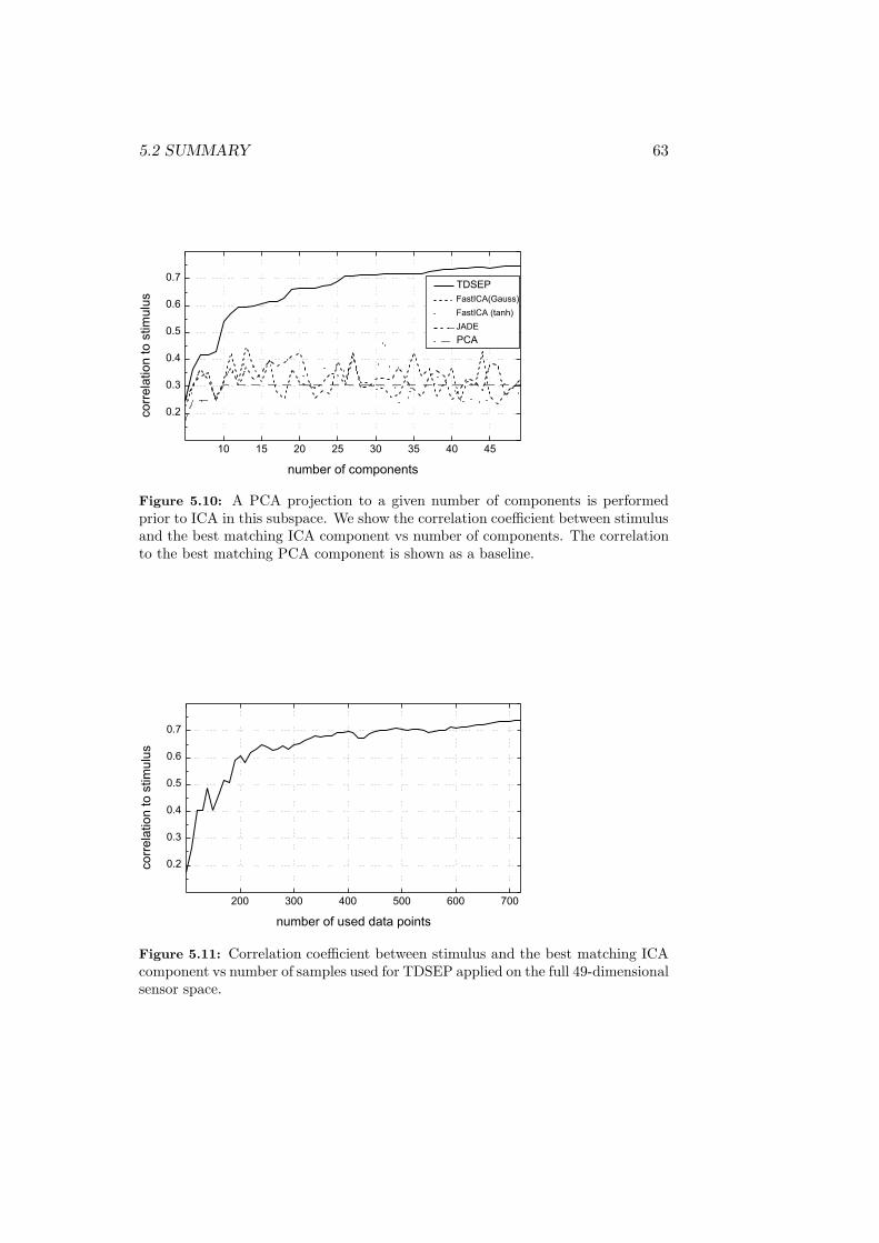
5.2 SUMMARY 63
10 15 20 25 30 35 40 45
0.2
0.3
0.4
0.5
0.6
0.7TDSEP
FastICA(Gauss)
FastICA (tanh)
JADE
PCA
corr
ela
tion to s
tim
ulu
s
number of components
Figure 5.10: A PCA projection to a given number of components is performedprior to ICA in this subspace. We show the correlation coefficient between stimulusand the best matching ICA component vs number of components. The correlationto the best matching PCA component is shown as a baseline.
200 300 400 500 600 700
0.2
0.3
0.4
0.5
0.6
0.7
corr
ela
tion to s
tim
ulu
s
number of used data points
Figure 5.11: Correlation coefficient between stimulus and the best matching ICAcomponent vs number of samples used for TDSEP applied on the full 49-dimensionalsensor space.

64 5 APPLICATIONS

Chapter 6
Conclusions
Here we summarize our main results and point out some pos-sibilities for future research.
6.1 Summary
In this thesis we addressed the problem of blind source separation (BSS)using approximate joint diagonalization (AJD) of a set of matrices. We haveshown that an AJD algorithm provides an efficient estimation procedurefor the mixing matrix of the BSS problem. Thus a general AJD methodis of great importance. As our main contribution, we proposed two newalgorithms to solve the AJD problem numerically. The specific structure ofthese algorithms implements a numerical optimization procedure on a matrixgroup by utilizing matrix exponential updates. As in classical optimizationmethods, the updating can be based on a gradient descent step or on aNewton step. The later is know for a faster convergence rate (quadraticrather than linear), however the computational burden in the classical caseis often prohibitively high.
The key features of our new algorithm called FFDiag are the use of alocal parameterization of the cost function combined with a further approx-imation, which results in a block-diagonal Hessian with 2 × 2 blocks whichallows for a closed form inverse and thus yields a highly efficient computationof the Newton update step.
Additional constraints, such as orthogonality, are not required by ouralgorithm, but if available, such constraints can be naturally incorporatedand yield further simplifications of the algorithm.
We have empirically observed that the approximative solution found bythe algorithm is of high quality for practical applications, and in particularfor BSS problems.
65
66 6 CONCLUSIONS
A series of comparisons of the FFDiag algorithm with state-of-the-art diagonalization algorithms was presented under a number of varyingconditions. The main conclusions of this comparative evaluation is thatour algorithm is competitive with the best algorithms (i.e. extended Jacobimethod and Pham’s algorithm) in situations where additional constraintseither on the class of solutions or the type of input data apply. In large-scale problems of non-orthogonal diagonalization FFDiag exhibits rapidconvergence relative to gradient-based methods such as Yeredor’s AC-DCalgorithm, which is the only AJD method applicable under the same gen-eral conditions, i.e. without assuming orthogonality of the diagonalizer orpositive-definiteness of the target matrices.
We also noticed that FFDiag may yield suboptimal solutions if thetarget matrices deviate extremely from a diagonalizable set. In this large-residual case it is recommended to modify the set of target matrices. Thisis the price that we have to pay to get the low computational complexityand the power to diagonalize matrices of dimensions in the hundreds ofrows/columns, without imposing overly restrictive, additional assumptions,in cases where the model holds (small residual case).
Nevertheless, we expect that FFDiag will become a versatile tool forhigh-dimensional data analysis by taking advantage of the low computa-tional cost to achieve good approximate solutions.
6.2 Future Work
6.2.1 Algorithms
Possible directions for future research are to further develop and tune relatedoptimization algorithms, for example to combine gradient and Newton stepsin a Levenberg-Marquardt or conjugate gradient scheme. In addition, itwould be worth studying the fundamental differences between the variousminimization criteria J1,J2 and J3, seeking for some guidelines for choosingthe most appropriate one.
Since the parameter of interest should be constrained to a particularmatrix group, e.g. the special orthogonal group SO(N) or the special lineargroup SL(N), the AJD problem should be treated as a non-linear optimiza-tion problem on a manifold with a group structure. It turns out that theterminology of differential geometry and matrix algebra provides the rightconcepts for the development of efficient numerical algorithms that preservethose important features and always stay on the group manifold (Cardoso,1998a). Thus, studying AJD algorithms as special cases of the isospectralflow methods in Helmke and Moore (1994); Hori (1999); Plumbley (2004)appears to be very promising.
Furthermore, it could be of interest to study the matrix exponentialupdates in the context of other Lie groups and their corresponding Lie al-

6.2 FUTURE WORK 67
gebras, which opens up new possibilities of research in the intersection ofoptimization, signal processing and machine learning.
6.2.2 Biomedical Applications
From the biomedical applications point of view it would be an interestinggoal for future research to incorporate prior knowledge into BSS models. Insome preliminary studies, it has been observed that, as one departs frompurely statistically based assumptions, one might get even closer to physi-ologically meaningful decompositions of electromagnetic brain signals. Onthe other hand, fitting neural sources in a classical framework, may be hardif some temporal overlap is present in their activations. Hence, a well bal-anced use of both, the model and appropriate priors, will yield a powerfulexploratory decomposition technique that is able to extract meaningful in-formation from high-dimensional biomedical data.
Furthermore it may be possible to apply the approximate joint diago-nalization techniques to other problems of neurobiological modeling such assparse coding in the visual cortex and taking advantage of an underlyinggroup structure.
6.2.3 Other Applications
BSS methods have also been successfully applied to a variety of problemswhich—beyond biomedical signal processing—include diverse fields as tele-communications, feature extraction for pattern recognition, financial time-series analysis, data mining or image processing (see e.g. Cardoso et al.(1999); Hyvarinen et al. (2001)).
For certain applications, including the famous cocktail-party problem inauditory perception (von der Malsburg and Schneider, 1986), the instanta-neous model in equation (2.1) is however too simplistic, since time-delaysin the signal propagation are no longer negligible. Extended models to dealwith such convolutive mixtures have been considered (e.g. Parra and Spence,2000; Lee et al., 1998; Murata et al., 2001) and are promising future appli-cations.

68 6 CONCLUSIONS
Appendix A
Notation
A.1 Abbreviations
AC-DC Alternating Columns Direct Centers (diagonalization algorithm)AJD Approximate Joint DiagonalizationBSS Blind Source SeparationCHESS CHaracteristic function Enabled Signal SeparationDOMUNG Diagonalization Of Matrices Using Natural GradientEEG Electroencephalogram ElectroencephalographyEVD Eigen Value DecompositionFastICA Fast Independent Component AnalysisFFDiag Fast Frobenius DiagonalizationFHG Fraunhofer GesellschaftFIRST Fraunhofer Institut fur Rechnerarchitektur und SoftwaretechnikICA Independent Component AnalysisIDA Intelligent Data AnalysisJADE Joint Approximate Diagonalization of Eigen-matricesMEG Magneto-encephalogram or Magneto-encephalographyMI Mutual InformationML Maximum LikelihoodMNG Magneto-neurogram or Magneto-neurographyMRI Magnetic Resonance ImagingOFI Optimal FilteringPCA Principal Component AnalysisPTB Physikalisch-Technische Bundesanstaltpdf probability density functionSQUID Superconducting Quantum Interference DeviceTDSEP Temporal Decorrelation SEParation
69

70 A NOTATION

A.2 MATHEMATICAL NOTATION 71
A.2 Mathematical Notation
Symbols
A, . . . ,Z matricesa, . . . , z vectorsa, b, . . . , z α, β, . . . , ω scalarsAT matrix transposeA−1 matrix inverseA−T the inverse of AT
A(m) matrix A in the m-th iterationAij matrix element of Adiag(A) diagonal matrix with same diagonal as AX random variableI identity matrixD diagonal matrixP permutation matrixA mixing matrixV demixing matrix or separating matrixX data matrixC covariance-like target matrix
Sets and Spaces
IR set of real numbersC set of complex numbers
IR(N×N) set of real matrices of dimension N ×NGL(N) General linear groupSL(N) Special linear groupO(N) Orthogonal group
Functions
EX{X} expected value w.r.t XφX,Y (τ) cross-correlation functioncum(·, . . . , ·) cumulant tensorMI(X,Y) mutual information between X and YH(X) Shannon entropy of XH(X—Y) conditional entropy of X given YO(N) measure of the complexity of an algorithm

72 A NOTATION

Appendix B
Some basic group theory
B.1 Matrix Lie Groups
The parameter space of the joint diagonalization problem (just as in therelated ICA case) is not arbitrary, but possess a very favorable structure,known as a matrix Lie group (Cardoso, 1998a; Hori, 1999; Akuzawa and Murata,2001; Plumbley, 2004). We have implicitly made use of this fact by intro-ducing the matrix exponential update.
In the following we briefly restate some theoretical concepts taken fromGrosche et al. (1995).
Definition (group). A set G is a group for the operation • if:
1. ∀A,B ∈ G ⇒ A •B ∈ G: G is closed.
2. ∀A,B,C ∈ G ⇒ (A • B) • C = A • (B •C): G obeys the associativelaw.
3. ∃I ∈ G so that ∀A ∈ G A • I = I •A = A: G has a unit element.
4. ∀A ∈ G ∃A−1 ∈ G so that A •A−1 = A−1 •A = I: Each element inG has an inverse.
The group is called Abelian or commutative if also holds:5. ∀A,B ∈ G ⇒ A •B = B •A
Definition (Lie group). A group G is said to be a Lie group if its multi-plication and inversion operation are continuous.
Definition (Matrix group). A subset of nonsingular matrices which areclosed under matrix multiplication and inversion is called a matrix group.
It turns out that every matrix group is in fact a Lie group, since the usualmatrix multiplication and matrix inversion are smooth maps. The reasonthat Lie groups are interesting is because this particular entity combines
73

74 B SOME BASIC GROUP THEORY
both algebraic and geometric structures. The most remarkable feature of aLie group is that the structure is the same in the neighborhood of each ofits elements. For this reason Lie group theory can provide powerful toolsfor designing and analyzing numerical optimization methods in structuredparameter spaces. For example, it is possible to confine an iterative numer-ical algorithm to a certain Lie group by imposing conditions on a relatedstructure, called a Lie algebra.
Definition (Lie algebra). The set of all tangents at identity of a Lie groupG forms a Lie algebra g, that is a linear space closed under commutation:
1. A,B ∈ g⇒ A + B ∈ g;
2. A ∈ g, λ ∈ IR⇒ λA ∈ g;
3. A,B ∈ g⇒ [A,B]def= AB−BA ∈ g
The most important relation for Lie groups and Lie algebras involves thematrix exponential function: If W belongs to a Lie algebra, then eW is amatrix that belongs to the corresponding Lie group. In other words, thereis an unique mapping from the Lie group to the Lie algebra and vice versa.For matrix Lie groups, this mapping is the matrix exponential.
PSfrag replacements
W
W
W
V(m)
V(m+1)
Lie algebraLie group
tangent space
eW
log
T GV(m) T GI0
Figure B.1: Concept of a Lie group method: The Lie algebra determines the local
structure of the Lie group via the exponential map.
Another important concept is the tangent space of a Lie group: it canbe shown that at the identity this tangent space has always the structure ofa Lie algebra (Helmke and Moore, 1994).
The important feature that we use in our algorithm is the fact that theLie algebra determines the local structure of the Lie group via the exponen-tial map. Thus we obtain a local parameterization of the group in terms ofelements of the algebra.

B.1 MATRIX LIE GROUPS 75
Examples of Lie Groups and Lie Algebras
The classical illustrating example is the unit circle in C. In this case theexponential function maps from the real line (the tangent space) to the circle(see Fig. B.2).
PSfrag replacements
1 + θeiθ
1
R
I
Figure B.2: Mapping from the real line to the circle.
Important examples of matrix Lie groups are:
• the General Linear Group GL(N) As indicated by the name,GL(N) is the most general matrix Lie group, in the sense that allother matrix Lie groups are subsets of GL(N). The corresponding Liealgebra gl(N) is IRN×N .
• the Special Linear Group SL(N) is the group of all matrices withdeterminant one. The dimension is N 2 − 1.
• the Orthogonal Group O(N) ) is the group of orthogonal N ×Nmatrices.
• the Special Orthogonal Group SO(N) is the subset of O(N) withdeterminant one. It has the dimension N(N − 1)/2.

76 B SOME BASIC GROUP THEORY

Bibliography
T. Akuzawa and N. Murata. Multiplicative nonholonomic Newton-like al-gorithm. Chaos, Solitons & Fractals, 12:785f, 2001.
S. I. Amari, T.-P. Chen, and A. Cichocki. Nonholonomic orthogonal learningalgorithms for blind source separation. Neural Computation, 12:1463–1484, 2000.
S. I. Amari and A. Cichocki. Adaptive blind signal processing – neuralnetwork approaches. Proceedings of the IEEE, 9:2026–2048, 1998.
S. I. Amari, A. Cichocki, and H. H. Yang. A new learning algorithm for blindsignal separation. In D.S. Touretzky, M.C. Mozer, and M.E. Hasselmo,editors, Advances in Neural Information Processing Systems (NIPS 95),volume 8, pages 882–893. The MIT Press, 1996.
S. I. Amari, S. Makino, and K. Matsuoka, editors. Proc. 4th InternationalSymposium on Independent Component Analysis and Blind Signal Separa-tion (ICA2003), 2003. URL http://ica2003.bsis.brain.riken.go.jp.
T. Back, K. Kohno, and K.A. Hossmann. Cortical negative DC deflectionsfollowing middle cerebral artery occlusion and KCl-induced spreading de-pression: effect on blood flow, tissue oxygenation and electroencephalo-gram. J. Cereb. Blood Flow Metab., 14(1):12–19, 1994.
A. J. Bell and T. J. Sejnowski. An information maximisation approach toblind separation and blind deconvolution. Neural Computation, 7:1129–1159, 1995.
A. Belouchrani, K. Abed Meraim, J.-F. Cardoso, and E. Moulines. A blindsource separation technique based on second order statistics. IEEE Trans.on SP, 45(2):434–44, Feb 1997.
A. Belouchrani and M. Amin. Blind source separation based on time-frequency signal representations. IEEE Trans. on Signal Processing, 46(11):2888–2897, 1998.
77
78 BIBLIOGRAPHY
A. Bunse-Gerstner, R. Byers, and V. Mehrmann. Numerical methods forsimultaneous diagonalization. SIAM Journal on Matrix Analysis and Ap-plications, 14(4):927–949, 1993.
J.-F. Cardoso. On the performance of orthogonal source separation algo-rithms. In Proc. EUSIPCO, pages 776–779, 1994.
J.-F. Cardoso. Infomax and maximum likelihood for source separation. IEEELetters on Signal Processing, 4:112–114, 1997.
J.-F. Cardoso. Learning in manifolds: the case of source separation. In Proc.SSAP ’98, 1998a.
J.-F. Cardoso. Multidimensional independent component analysis. In Proc.ICASSP ’98. Seattle, 1998b.
J.-F. Cardoso. High-order contrasts for independent component analysis.Neural Computation, 11(1):157–192, January 1999.
J.-F. Cardoso. The three easy routes to independent component analysis;contrasts and geometry. In Proc. ICA 2001, San Diego, 2001.
J.-F. Cardoso, Ch. Jutten, and Ph. Loubaton, editors. First InternationalWorkshop on Independent Component Analysis and Signal Separation,Aussois, France, Jan 1999.
J.-F. Cardoso and A. Souloumiac. Blind beamforming for non Gaussiansignals. IEE Proceedings F, 140(6):362–370, 1993.
J.-F. Cardoso and A. Souloumiac. Jacobi angles for simultaneous diagonal-ization. SIAM J. Mat. Anal. Appl., 17(1):161–164, January 1996.
Q. Chen, M. Chopp, H. Chen, and N. Tepley. Magnetoencephalography offocal ischemia in rats. Stroke, 23(9):1299–1303, Sep 1992.
S. Choi, A. Cichocki, and A. Belouchrani. Blind separation of second-ordernonstationary and temporally colored sources. In Proc. IEEE Workshopon Statistical Signal Processing (IEEE SSP 2001), pages 444–447, Singa-pore, 2001.
P. Comon. Independent component analysis, a new concept? Signal Pro-cessing, Elsevier, 36(3):287–314, 1994.
T.M. Cover and J.A. Thomas. Elements of information theory. John Wiley& Sons, Inc., New York, 1991.
G. Curio, S.M. Erne, M. Burghoff, K.-D. Wolff, and A. Pilz. Non-invasiveneuromagnetic monitoring of nerve and muscle injury currents. Electroen-cephalography and clinical Neurophysiology, 89(3):154–160, 1993.

BIBLIOGRAPHY 79
L. de Lathauwer. Signal Processing by Multilinear Algebra. PhD thesis,Faculty of Engineering, K. U. Leuven, Leuven, Belgium, 1997.
D. Drung. The PTB 83-SQUID-system for biomagnetic applications in aclinic. IEEE Trans. Appl. Supercond., 5(2):2112–2117, 1995.
B. Flury and W. Gautschi. An algorithm for simultaneous orthogonal trans-formation of several positive definite symmetric matrices to nearly diag-onal form. SIAM Journal on Scientific and Statistical Computing, 7(1):169–184, January 1986.
K. Fukunaga. Statistical Pattern Recognition. Academic Press, 1990. 2ndedition.
A. R. Gardner-Medwin, N. Tepley, G. L. Barkley, J. E. Moran, S. Nagel-Leiby, R. T. Simkins, and K. M. A. Welch. Magnetic fields associatedwith spreading depression in anaesthetized rabbits. Brain Res., 540(1-2):153–158, Feb 1991.
G. H. Golub and C. F. van Loan. Matrix Computation. The Johns HopkinsUniversity Press, London, 1989.
G. Grosche, V. Ziegler, D. Ziegler, and E. Zeidler, editors. Bronstein-Semendjajew - Teubner-Taschenbuch der Mathematik - Teil II - Neubear-beitung, chapter 17. Liegruppen, Liealgebren und Elementarteilchen—Mathematik der Symmetrie, pages 643 – 704. B.G.Teubner Verlags-gesellschaft, Leipzig, 1995.
S. Harmeling, A. Ziehe, M. Kawanabe, and K.-R. Muller. Kernel featurespaces and nonlinear blind souce separation. In Advances in Neural In-formation Processing Systems 14, pages 761–768, 2001.
S. Harmeling, A. Ziehe, M. Kawanabe, and K.-R. Muller. Kernel-basednonlinear blind source separation. Neural Computation, 15(5):1089–1124,May 2003.
S. Haykin, editor. Unsupervised Adaptive Filtering, Vol. 1: Blind SourceSeparation. Wiley, 2000.
U. Helmke and J.B. Moore. Optimization and Dynamical Systems. SpringerVerlag, 1994.
G. Hori. Joint diagonalization and matrix differential equations. In Proc. ofNOLTA’99, pages 675–678. IEICE, 1999.
R. A. Horn and C. R. Johnson. Matrix Analysis. Cambridge UniversityPress., Cambridge, 1985.
80 BIBLIOGRAPHY
A. Hyvarinen, J. Karhunen, and E. Oja. Independent Component Analysis.John Wiley & Sons, New York, 2001.
A. Hyvarinen and E. Oja. A fast fixed-point algorithm for independentcomponent analysis. Neural Computation, 9(7):1483–1492, 1997.
C. G. Jacobi. Uber ein leichtes Verfahren, die in der Theorie der Sacu-larstorungen vorkommenden Gleichungen numerisch aufzulosen. Crelle J.reine angew. Mathematik, 30:51–94, 1846.
M. Joho and H. Mathis. Joint diagonalization of correlation matrices byusing gradient methods with application to blind signal separation. InProc. of IEEE Sensor Array and Multichannel Signal Processing Work-shop SAM, pages 273–277, 2002.
M. Joho and K. Rahbar. Joint diagonalization of correlation matrices byusing Newton methods with application to blind signal separation. InProc. of IEEE Sensor Array and Multichannel Signal Processing Work-shop SAM, pages 403–407, 2002.
Ch. Jutten and J. Herault. Blind separation of sources, part I: An adaptivealgorithm based on neuromimetic architecture. Signal Processing, 24:1–10, 1991.
L. V. Kantorovich. On Newton’s method. In Trudy Mat. Inst. Steklov,volume 28, pages 104–144. Interperiodica publishing, 1949. Translation:Selected Articles in Numerical Analysis by C. D. Benster, 104.1–144.2.
B. Laheld and J.-F. Cardoso. Equivariant adaptive source separation. IEEETrans. on Signal Processing, 44(12):3017–3030, 1996.
T. W. Lee, T. P. Jung, S. Makeig, and T. J. Sejnowski, editors. Proc. 3rdInternational Conference on Independent Component Analysis and BlindSignal Separation, San Diego, USA, 2001.
T.W. Lee, A. Ziehe, R. Orglmeister, and T. .J. Sejnowski. Combining time-delayed decorrelation and ICA: Towards solving the cocktail party prob-lem. In Proc. ICASSP98, volume 2, pages 1249–1252, Seattle, May 1998.
K. Levenberg. A method for the solution of certain non-linear problems inleast squares. Quarterly of Applied Mathematics, pages 164–168, 1944.
B.-M. Mackert, J. Mackert, G. Wubbeler, F. Armbrust, K.-D. Wolff,M. Burghoff, L. Trahms, and G. Curio. Magnetometry of injury currentsfrom human nerve and muscle specimens using superconducting quantuminterferences devices. Neuroscience Letters, 262(3):163–166, Mar 1999a.
BIBLIOGRAPHY 81
B.-M. Mackert, G. Wubbeler, M. Burghoff, P. Marx, L. Trahms, and G. Cu-rio. Non-invasive long-term recordings of cortical ’direct current’ (DC-)activity in humans using magnetoencephalography. Neuroscience Letters,273(3):159–162, Oct 1999b.
S. Makeig, A.J. Bell, T.-P. Jung, and T.J. Sejnowski. Independent com-ponent analysis of electroencephalographic data. In David S. Touretzky,Michael C. Mozer, and Michael E. Hasselmo, editors, Advances in Neu-ral Information Processing Systems (NIPS’95), volume 8, pages 145–151.The MIT Press, 1996.
S. Makeig, T-P. Jung, D. Ghahremani, A.J. Bell, and T.J. Sejnowski. Blindseparation of event-related brain responses into independent components.Proc. Natl. Acad. Sci. USA, 94:10979–10984, 1997.
D. W. Marquardt. An algorithm for least-squares estimation of nonlinearparameters. Journal of SIAM, 11(2):431–441, jun 1963.
K. Matsuoka, M. Ohya, and M. Kawamoto. A neural net for blind separationof nonstationary signals. Neural Networks, 8:411–419, 1995.
F. C. Meinecke, A. Ziehe, M. Kawanabe, and K.-R. Muller. Estimatingthe reliability of ICA projections. In Advances in Neural InformationProcessing Systems 14, pages 1181–1188, 2001.
F. C. Meinecke, A. Ziehe, M. Kawanabe, and K.-R. Muller. A ResamplingApproach to Estimate the Stability of one- or multidimensional Inde-pendent Components. IEEE Trans. on Biomedical Engineering, 49(12):1514–1525, 2002.
F. C. Meinecke, A. Ziehe, J. Kurths, and K.-R. Muller. Measuring phasesynchronization of superimposed signals. Physical Review Letters, 94(8):084102, March 2005.
L. Molgedey and H. G. Schuster. Separation of a mixture of independentsignals using time delayed correlations. Physical Review Letters, 72(23):3634–3637, 1994.
E. Moreau. A generalization of joint-diagonalization criteria for source sep-aration. IEEE Trans. on Signal Processing, 49(3):530–541, March 2001.
K.-R. Muller, N. Murata, A. Ziehe, and S.-I. Amari. On-line learning inneural networks, chapter On-line learning in Switching and Drifting en-vironments with application to blind source separation, pages 93–110.Cambridge University Press, 1998.
K.-R. Muller, R. Vigario, F. C. Meinecke, and A. Ziehe. Blind source separa-tion techniques for decomposing event-related brain signals. InternationalJournal of Bifurcation and Chaos, 14(2):773–791, 2004.
82 BIBLIOGRAPHY
N. Murata, S. Ikeda, and A. Ziehe. An approach to blind source separationbased on temporal structure of speech signals. Neurocomputing, 41(1-4):1–24, August 2001.
N. Murata, M. Kawanabe, A. Ziehe, K.-R. Muller, and S. I. Amari. On-linelearning in changing environments with applications in supervised andunsupervised learning. Neural Networks, 15(4-6):743–760, 2002.
B. Noble and W. Daniel. Applied matrix algebra. Prentice Hall, Inc., Engle-wood Cliffs, NJ, 1977.
G. Nolte, A. Ziehe, and K. R. Muller. Noise robust estimates of correlationdimension and K2 entropy. Physical review E, 64(1):016112, June 2001.
P. Pajunen and J. Karhunen, editors. Proceedings of the Second Interna-tional Workshop on Independent Component Analysis and Blind SourceSeparation. Helsinki Univ. of Technology, Lab. of Computer and Informa-tion Science, Espoo, Finland, June 19-22, 2000. 647 pages.
C. Pantev, C. Eulitz, S. Hampson, B. Ross, L.E., and Roberts. The auditoryevoked off response: source and comparison with the on and the sustainedresponses. Ear & Hearing, 17(3):255–265, Jun 1996.
L. Parra and C. Spence. Convolutive blind source separation of non-stationary sources. IEEE Trans. on Speech and Audio Processing, 8(3):320–327, 2000.
L. Parra, C. Spence, P. Sajda, A. Ziehe, and K.-R. Muller. Unmixing hyper-spectral data. In Sara A. Solla, Todd K. Leen, and Klaus-Robert Muller,editors, Advances in Neural Information Processing Systems 12, pages942–948, 1999.
D.-T. Pham. Joint approximate diagonalization of positive definite matrices.SIAM J. on Matrix Anal. and Appl., 22(4):1136–1152, 2001.
D.-T. Pham. Exploiting source non-stationary and coloration in blind sourceseparation. In Proceedings of the DSP2002 conference, pages 151–154,Santorini, Greek, July 2002.
D.-T. Pham and J.-F. Cardoso. Blind separation of instantaneous mixturesof non-stationary sources. In Proc. Int. Workshop on Independent Com-ponent Analysis and Blind Signal Separation (ICA2000), pages 187–193,Helsinki, Finland, 2000.
D.-T. Pham and J.-F. Cardoso. Blind separation of instantaneous mixturesof non stationary sources. IEEE Trans. Sig. Proc., 49(9):1837–1848, 2001.
BIBLIOGRAPHY 83
D.-T. Pham and P. Garrat. Blind separation of mixture of independentsources through a quasi-maximum likelihood approach. IEEE Trans. onSignal Processing, 45(7):1712–1725, 1997.
T.W. Picton, D.L. Woods, and G.B. Proulx. Human auditory sustainedpotentials: part I and II. Electroencephalography and clinical Neurophys-iology, 45(2):186–210, Aug 1978.
M. D. Plumbley. Lie group methods for optimization with orthogonalityconstraints. In Proc. ICA 2004, volume 3195 of Lecture Notes in ComputerScience, pages 1245 – 1252, Oct 2004.
W.H. Press, S.A. Teukolsky, W.T. Vetterling, and B.P. Flannery. NumericalRecipies in C. Cambridge University Press., Cambridge, 1992.
C. G. Puntonet and A. Prieto, editors. Independent Component Analysisand Blind Signal Separation: Fifth International Conference (ICA 2004),volume 3195 of Lecture Notes in Computer Science, Granada, Spain, 2004.Springer Verlag.
L. Tong, V.C. Soon, and Y. Huang. Indeterminacy and identifiability ofidentification. IEEE Trans. on Circuits and Systems, 38(5):499–509,1991.
M. Uusitalo and R. Ilmoniemi. Signal-space projection method for separat-ing meg or eeg into components. Med. & Biol. Eng. & Comput., 10(35):135–140, Oct. 1997.
A.-J. van der Veen. Joint diagonalization via subspace fitting techniques. InProc. ICASSP, volume 5, 2001.
R. Vigario, V. Jousmaki, M. Hamalainen, R. Hari, and E. Oja. Independentcomponent analysis for identification of artifacts in magnetoencephalo-graphic recordings. In Michael I. Jordan, Michael J. Kearns, and Sara A.Solla, editors, Advances in Neural Information Processing Systems, vol-ume 10. The MIT Press, 1998.
R. Vigario, A. Ziehe, K.-R. Muller, J. Sarela, E. Oja, V. Jousmaki,G. Wubbeler, L. Trahms, B.-M. Mackert, and G. Curio. Advances in Ex-ploratory analysis and data modeling in functional neuroimaging, chapterBlind decomposition of multimodal and DC evoked responses. MIT Press,Cambridge MA., December 2002. ISBN 0-262-19481-3.
R. Vigario, J. Sarela, V. Jousmaki, M. Hamalainen, and E. Oja. Independentcomponent approach to the analysis of EEG and MEG recordings. IEEEtransactions on biomedical engineering, 47(5):589–593, 2000.

84 BIBLIOGRAPHY
C. von der Malsburg and W. Schneider. A neural cocktail-party processor.Biological Cybernetics, 54:29–40, 1986.
H. A. Van der Vorst and G. H. Golub. 150 years old and still alive: Eigen-problems. In The State of the Art in Numerical Analysis, volume 63,pages 93–120. Oxford University Press, 1997.
O. Weiss, A. Ziehe, and H. Herzel. Optimizing property codes in proteindata reveals structural characteristics. In Proc. International Conferenceon Artificial Neural Networks, pages 245–252. Springer Verlag, 2003.
H.-C. Wu and J.C. Principe. Simultaneous diagonalization in the frequencydomain (SDIF) for source separation. In Proc. First International Con-ference on Independent Component Analysis and Blind Source SeparationICA 99, pages 245–250, Aussois, France, January 11–15, 1999.
G. Wubbeler, B.-M. Mackert, F. Armbrust, M. Burghoff, P. Marx, G. Curio,and L. Trahms. Measuring para-DC biomagnetic fields of the head usinga horizontal modulated patient cot. Biomed Tech (Berl), Suppl(43):232–233, 1999. in german.
G. Wubbeler, J. Mackert, F. Armbrust, M. Burghoff, B.-M. Mackert, K.-D.Wolff, J. Ramsbacher, G. Curio, and L. Trahms. SQUID measurementsof human nerve and muscle near-DC injury-currents using a mechanicalmodulation of the source position. Applied Superconductivity, 6(10-12):559–565, 1998.
G. Wubbeler, A. Ziehe, B.-M. Mackert, K.-R. Muller, L. Trahms, and G. Cu-rio. Independent component analysis of non-invasively recorded corticalmagnetic DC-fields in humans. IEEE Transactions on Biomedical Engi-neering, 47(5):594–599, 2000.
A. Yeredor. Blind source separation via the second characteristic function.Signal Processing, 80(5):897–902, 2000.
A. Yeredor. Non-orthogonal joint diagonalization in the least-squares sensewith application in blind source separation. IEEE Transactions on SignalProcessing, 50(7):1545–1553, July 2002.
A. Yeredor, A. Ziehe, and K.-R. Muller. Approximate joint diagonalizationusing a natural gradient approach. In Proc. ICA 2004, Lecture Notes inComputer Science, pages 89–96, 2004.
M. Zibulevsky. Relative Newton method for quasi-ML blind source separa-tion. In Proc. 4th Intern. Symp. on Independent Component Analysis andBlind Signal Separation (ICA2003), pages 897–902, Nara, Japan, 2003.

BIBLIOGRAPHY 85
A. Ziehe, M. Kawanabe, S. Harmeling, and K.-R. Muller. Blind separation ofpost-nonlinear mixtures using gaussianizing transformations and temporaldecorrelation. In Proc. ICA 2003, pages 269–274, Nara, Japan, Apr 2003a.
A. Ziehe, M. Kawanabe, S. Harmeling, and K.-R. Muller. Blind separationof post-nonlinear mixtures using linearizing transformations and temporaldecorrelation. Journal of Machine Learning Research, 4:1319–1338, Dec2003b.
A. Ziehe, P. Laskov, K.-R. Muller, and G. Nolte. A linear least-squaresalgorithm for joint diagonalization. In Proc. ICA 2003, pages 469–474,Nara, Japan, Apr 2003c.
A. Ziehe, P. Laskov, G. Nolte, and K.-R. Muller. A fast algorithm for jointdiagonalization with non-orthogonal transformations and its applicationto blind source separation. Journal of Machine Learning Research, 5:777–800, 2004.
A. Ziehe and K.-R. Muller. TDSEP–an efficient algorithm for blind sep-aration using time structure. In Proc. Int. Conf. on Artificial NeuralNetworks (ICANN’98), pages 675–680, Skovde, Sweden, 1998.
A. Ziehe, K.-R. Muller, G. Nolte, B.-M. Mackert, and G. Curio. Artifact re-duction in magnetoneurography based on time-delayed second-order cor-relations. IEEE Trans. Biomed. Eng., 47(1):75–87, January 2000a.
A. Ziehe, G. Nolte, G. Curio, and K.-R. Muller. OFI: Optimal filteringalgorithms for source separation. In Proc. Int. Workshop on IndependentComponent Analysis and Blind Signal Separation (ICA2000), pages 127–132, Helsinki, Finland, 2000b.
A. Ziehe, G. Nolte, T. Sander, K.-R. Muller, and G. Curio. A comparisonof ICA-based artifact reduction methods for MEG. In Jukka Nenonen,editor, Recent Advances in Biomagnetism, Proc. of the 12th Interna-tional conference on Biomagnetism, pages 895–898, Espoo,Finland, 2001.Helsinki University of Technology.