Embed Size (px)
Citation preview
1092 IEEE TRANSACTIONS ON VEHICULAR TECHNOLOGY, VOL. 50, NO. 4, JULY 2001
Blind Turbo Equalization in Gaussianand Impulsive Noise
Xiaodong Wang, Member, IEEE,and Rong Chen
Abstract—We consider the problem of simultaneous parameterestimation and restoration of finite-alphabet symbols that areblurred by an unknown linear intersymbol interference (ISI)channel and contaminated by additive Gaussian or non-Gaussianwhite noise with unknown parameters. Non-Gaussian noise isfound in many wireless channels due to impulsive phenomena ofradio-frequency interference. Bayesian inference of all unknownquantities is made from the blurred and noisy observations.The Gibbs sampler, a Markov chain Monte Carlo procedure,is employed to calculate the Bayesian estimates. The basic ideais to generate ergodic random samples from the joint posteriordistribution of all unknowns and then to average the appropriatesamples to obtain the estimates of the unknown quantities. BlindBayesian equalizers based on the Gibbs sampler are derived forboth Gaussian ISI channel and impulsive ISI channel. A salientfeature of the proposed blind Bayesian equalizers is that they canincorporate the a priori symbol probabilities, and they produceas output the a posteriorisymbol probabilities. (That is, they are“soft-input soft-output” algorithms.) Hence, these methods arewell suited for iterative processing in a coded system, which allowsthe blind Bayesian equalizer to refine its processing based on theinformation from the decoding stage and vice versa—a receiverstructure termed asblind turbo equalizer.
Index Terms—Bayesian inference, blind equalization, Gibbssampler, impulsive noise, iterative processing.
I. INTRODUCTION
I N a band-limited digital communication system, thetransmitted digital symbols are distorted by the base-band
equivalent discrete-time linear finite impulse response (FIR)channel, causing intersymbol interference (ISI). Blind equal-ization refers to the reconstruction of transmitted symbolsbased on the noise-corrupted channel output without knowingthe underlying FIR channel. The traditional approach toblind equalization in digital communications is to use alinear equalizer, i.e., an FIR transversal filter. Two familiesof methodologies for blind adaptation of a linear equalizerare the high-order statistics (HOS)-based techniques, (suchas the Bussgang methods and the polyspectral methods), andthe second-order statistics (SOS)-based techniques, (such asthe cyclostationarity-based methods and the subspace-basedmethods). Discussions on these methodologies can be found in
Manuscript received November 22, 1999; revised January 23, 2001. Thiswork was supported in part by the Interdisciplinary Research Initiatives Pro-gram, Texas A&M University. X. Wang was supported in part by NSF GrantCAREER CCR-9875314. R. Chen was supported in part by the U.S. NationalScience Foundation under Grant DMS 9626113.
X. Wang is with the Department of Electrical Engineering, Texas A&M Uni-versity, College Station, TX 77843 USA (e-mail: [email protected]).
R. Chen is with the Department of Information and Decision Sciences, Uni-versity of Illinois at Chicago, Chicago, IL 60607 USA.
Publisher Item Identifier S 0018-9545(01)04892-7.
the articles collected in [15] and the more recent surveys [16],[43].
Since a linear equalizer may perform poorly in a severeISI channel, some recent work has addressed nonlinear blindequalization techniques. For example, the algorithms in [21],[25], [26], [40] employ a sequence estimator and a bank ofchannel estimators and alternatively optimize with respectto data and channel. Sequence estimation is performed by ablind search of a modified trellis and channel estimation isaccomplished by conditioning on survivor sequences in thetrellis and constructing the corresponding maximum likelihoodor minimum mean-square error channel estimate. Similariterative methods for joint sequence detection and channel esti-mation are also found in [17], [27] and it is shown in [27] thatthese procedures are based on the expectation-maximization(EM) algorithm. Symbol-by-symbol maximuma posterioriprobability (MAP)-based blind equalization schemes have alsobeen considered. For instance, Bayesian blind equalizationtechniques are proposed in [22], [26], which combine recursivechannel estimation with the MAP and the Bayesian decisionfeedback equalization methods for known channels introducedin [1]. Another Bayesian blind equalization method is proposedin [30], which is a Kalman-filter-like updating algorithm forjoint symbol and channel estimation.
To date most of the work on equalization and blind equaliza-tion assumes that the channel ambient noise is Gaussian. How-ever, in many physical channels such as urban and indoor radiochannels [5], [6], [34], [35], [37] and underwater acoustic chan-nels [8], [36], the ambient noise is known through experimentalmeasurements to be decidedly non-Gaussian, due to the impul-sive nature of the man-made electromagnetic interference and agreat deal of natural noise as well. (For recent measurement re-sults of impulsive noise in outdoor/indoor mobile and portableradio communications, see [5], [6] and the references therein.)It is widely known that linear signal processing procedures areineffective in combating non-Gaussian noise [28]. Hence, non-linear equalizers are necessary for impulsive ISI channels. Afew recent works addresstraining-basednonlinear equalizationtechniques in impulsive channels. For example, in [9], [29] non-linear equalizers based respectively on the radial basis functionnetwork and the EM algorithm are proposed.
Recently, iterative (“turbo”) processing techniques havereceived considerable attention following the discovery of thepowerful turbo codes [3], [4]. The so called turbo-principle canbe successfully applied to many detection/decoding problemssuch as serial concatenated decoding, equalization, codedmodulation, multi-user detection and joint source and channeldecoding [24]. Turbo equalization was first proposed in [14],where it is assumed that the channel coefficients are known. In[45], a low-complexity turbo multi-user receiver is developed
0018–9545/01$10.00 © 2001 IEEE
WANG AND CHEN: BLIND TURBO EQUALIZATION IN GAUSSIAN AND IMPULSIVE NOISE 1093
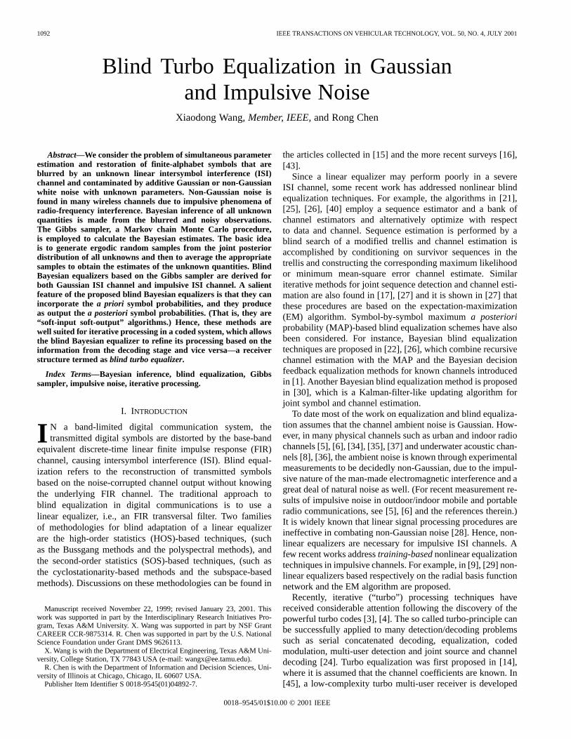
Fig. 1. A channel-coded communication system signaling through an intersymbol interference (ISI) channel with additive ambient noise.
for joint equalization and multi-user detection in CDMAsystems, where it is also assumed that the user channels areknown to the receiver.
In this paper, we present novel Bayesian blind equalizationtechniques for both Gaussian and impulsive ISI channels. Theabovementioned previous “Bayesian” equalization schemes,e.g., [22], [26], [30], all make various approximating assump-tions in deriving the equalizers and, therefore, they are nottrueBayesian procedures. We consider Bayesian inference of allunknown quantities (e.g., channel states, symbol values, noiseparameters) from the ISI-corrupted and noisy observations.A Markov chain Monte Carlo procedure called the Gibbssampler is employed to calculate the Bayesian estimates. Theperformance of the proposed blind Bayesian equalizers isdemonstrated via simulations. Another salient feature of theproposed methods is that being soft-input soft-output demod-ulation algorithms, they can be used in conjunction with softchannel decoding algorithm, to accomplish iterative joint blindequalization and decoding—so-calledblind turbo equalization.
The rest of the paper is organized as follows. In Section II,the system under study is described. In Section III, some back-ground material on the Gibbs sampler is provided. The problemsof blind Bayesian equalization of Gaussian and impulsive ISIchannels are treated in Sections IV and V respectively. In Sec-tion VI, a blind turbo equalization scheme is presented. Somediscussions are found in Section VII. Simulation results are pro-vided in Section VIII. Finally, Section IX contains the conclu-sions.
II. SYSTEM DESCRIPTION
We consider a channel-coded communication systemsignaling through an intersymbol interference (ISI) channelwith additive ambient noise. The block diagram of the trans-mitter-end of such a system is shown in Fig. 1. The binaryinformation bits are encoded using some channel code(e.g., block code, convolutional code, or turbo code), resultingin a code bit stream . A code bit interleaver is used toreduce the influence of the error bursts at the input of thechannel decoder. The interleaved code bits are thenpassed to a linear modulator, wherecode bits are mappedto one symbol. (e.g., PSK modulation or QAM modulation),yielding complex data symbols . Each data symbol is thentransmitted through an ISI channel. Suppose that a block of
symbols are transmitted. The discrete-time input–outputrelationship of the ISI channel is represented by the followinglinear finite impulse response (FIR) model
(1)
In (1), , and are, respectively, the received signal, thetransmitted symbol, and ambient noise sample at time; is thelength of the channel memory; is the size of the transmittedsymbol block; are the complex coefficients of theISI channel; denotes the conjugate transpose operation; and
, .It is assumed that the complex symbols are in-
dependent and they are drawn from a finite alphabet set. Define the following a priori
probabilities of symbol
(2)
Note that when no prior information is available, then, i.e., all symbols are equally likely.
It is further assumed that the additive ambient channel noiseis a sequence of zero-mean independent and identically
distributed (i.i.d.) complex random variables, and it is indepen-dent of the symbol sequence . In this paper, we considertwo types of noise distributions corresponding to the additiveGaussian noise and the additive impulsive noise, respectively.For the former case, the noise sampleis assumed to have acomplex Gaussian distribution, i.e.,
(3)
where is the noise variance. For the latter case, the noisesample is assumed to have a two-term Gaussian mixture dis-tribution, i.e.,
(4)
with and . Here, the term rep-resents the nominal ambient noise and the term rep-resents an impulsive component, withrepresenting the proba-bility that impulses occur. The total noise variance under distri-bution (4) is given by
(5)
Denote . In Sections IV and V, weconsider the problem of estimating thea posterioriprobabilitiesof the transmitted symbols
(6)
based on the received signals and the prior information, without knowing the channel and the noise
parameters (i.e., for Gaussian noise; , and forimpulsive noise). Thesea posterioriprobabilities are then usedby the channel decoder to decode the information bitsshown in Fig. 1, which will be discussed in Section VI.
1094 IEEE TRANSACTIONS ON VEHICULAR TECHNOLOGY, VOL. 50, NO. 4, JULY 2001
III. T HE GIBBS SAMPLER
Let be a vector of unknown parameters andlet be the observed data. Suppose that we are interested infinding thea posteriorimarginal distribution of some parameter,say , conditioned on the observation, i.e., ,
. Direct evaluation involves integrating out the rest of theparameters from the jointa posterioridensity, i.e.,
(7)
In most cases, such a direct evaluation is computationalinfeasible, especially when the parameter dimensionislarge. The Gibbs sampler [18] is a Monte Carlo procedure fornumerical evaluation of the above multidimensional integral.The basic idea is to generate random samples from the jointposterior distribution and then to estimate any marginaldistribution using these samples. Given the initial values
, this algorithm iterates the followingloop.
• Draw sample from .• Draw sample from
...
• Draw sample from .The convergence behavior of the Gibbs sampler is investigatedin [10], [18], [20], [33], [39], and [42] and general conditionsare given for the following two results:
• the distribution of converges geometrically to ,as ;
• , as ,for any integrable function .
The Gibbs sampler requires an initial transient period to con-verge to equilibrium. The initial period of length is knownas the “burning-in” period and the first samples should al-ways be discarded.
IV. BLIND BAYESIAN EQUALIZATION IN GAUSSIAN NOISE
In this section, we consider the problem of computing theaposteriorisymbol probabilities in (6), under the assumption thatthe ambient noise distribution is complex Gaussian. That is, theprobability density function (pdf) of in (1) is given by
(8)
Denote . The problem is solvedunder a Bayesian framework. First, the unknown quantities,
and are regarded as realizations of random variables withsome prior distributions. The Gibbs sampler, is then employedto calculate the maximuma posteriori (MAP) estimates ofthese unknowns.
A. Bayesian Inference
Assume that the unknown quantities, , and are inde-pendent of each other and have prior distributions , ,
and , respectively. Since is white and Gaussian,using (1) and (8), the joint posterior distribution of these un-known quantities based on the received signaltakes the form
(9)
Thea posterioriprobabilities (6) of the transmitted symbols canthen be calculated from the joint posterior distribution (9) ac-cording to
(10)
Clearly, the computation in (10) involves multidimen-sional integrals, which is certainly infeasible for any practicalimplementations. To avoid the direct evaluation of the Bayesianestimate (10), we resort to the Gibbs sampler discussed in Sec-tion III. The basic idea is to generate ergodic random samples
: from the posterior distribu-tion (9), and then to average to obtain anapproximation of thea posterioriprobabilities in (10).
B. Prior Distributions
1) General Considerations:a) Noninformative priors: In Bayesian analysis, prior
distributions are used to incorporate the prior knowledgeabout the unknown parameters. When such prior knowledgeis limited, the prior distributions should be chosen such thatthey play a minimal role in the posterior distribution. Suchpriors are termed asnoninformative. The rationale for usingnoninformative prior distributions is to “let the data speak forthemselves,” so that inferences are unaffected by informationexternal to current data.
b) Conjugate priors: Another consideration in the selec-tion of the prior distributions is to simplify computations. Tothat end,conjugate priorsare usually used to obtain simple an-alytical forms for the resulting posterior distributions. The prop-erty that the posterior distribution follows the same parametricform as the prior distribution is called conjugacy. The conjugatefamily of distributions is mathematically convenient in that theposterior distribution follows a known parametric form. Finally,to make the Gibbs sampler more computationally efficient, thepriors should also be chosen such that the conditional posteriordistributions are easy to simulate.
For an introductory treatment of the Bayesian philosophy, in-cluding the selection of prior distributions (see [7], [19], [31]).
2) Prior Distributions of the Unknowns:Following the gen-eral guidelines in Bayesian analysis [7], [19], [31], we choosethe conjugate prior distributions for the unknown parameters
, and as follows.
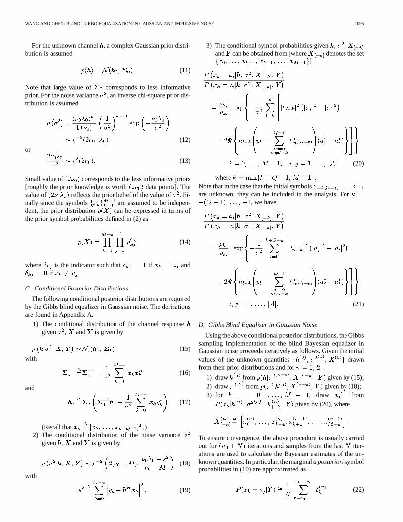
WANG AND CHEN: BLIND TURBO EQUALIZATION IN GAUSSIAN AND IMPULSIVE NOISE 1095
For the unknown channel, a complex Gaussian prior distri-bution is assumed
(11)
Note that large value of corresponds to less informativeprior. For the noise variance , an inverse chi-square prior dis-tribution is assumed
(12)
or
(13)
Small value of corresponds to the less informative priors[roughly the prior knowledge is worth data points]. Thevalue of reflects the prior belief of the value of . Fi-nally since the symbols are assumed to be indepen-dent, the prior distribution can be expressed in terms ofthe prior symbol probabilities defined in (2) as
(14)
where is the indicator such that if andif .
C. Conditional Posterior Distributions
The following conditional posterior distributions are requiredby the Gibbs blind equalizer in Gaussian noise. The derivationsare found in Appendix A.
1) The conditional distribution of the channel responsegiven , and is given by
(15)
with
(16)
and
(17)
(Recall that .)2) The conditional distribution of the noise variance
given , and is given by
(18)
with
(19)
3) The conditional symbol probabilities given, ,and can be obtained from [where denotes the set
]
(20)
where .Note that in the case that the initial symbolsare unknown, they can be included in the analysis. For
, we have
(21)
D. Gibbs Blind Equalizer in Gaussian Noise
Using the above conditional posterior distributions, the Gibbssampling implementation of the blind Bayesian equalizer inGaussian noise proceeds iteratively as follows. Given the initialvalues of the unknown quantities drawnfrom their prior distributions and for
1) draw from given by (15);2) draw from given by (18);3) for , draw from
given by (20), where
To ensure convergence, the above procedure is usually carriedout for iterations and samples from the last iter-ations are used to calculate the Bayesian estimates of the un-known quantities. In particular, the marginala posteriorisymbolprobabilities in (10) are approximated as
(22)
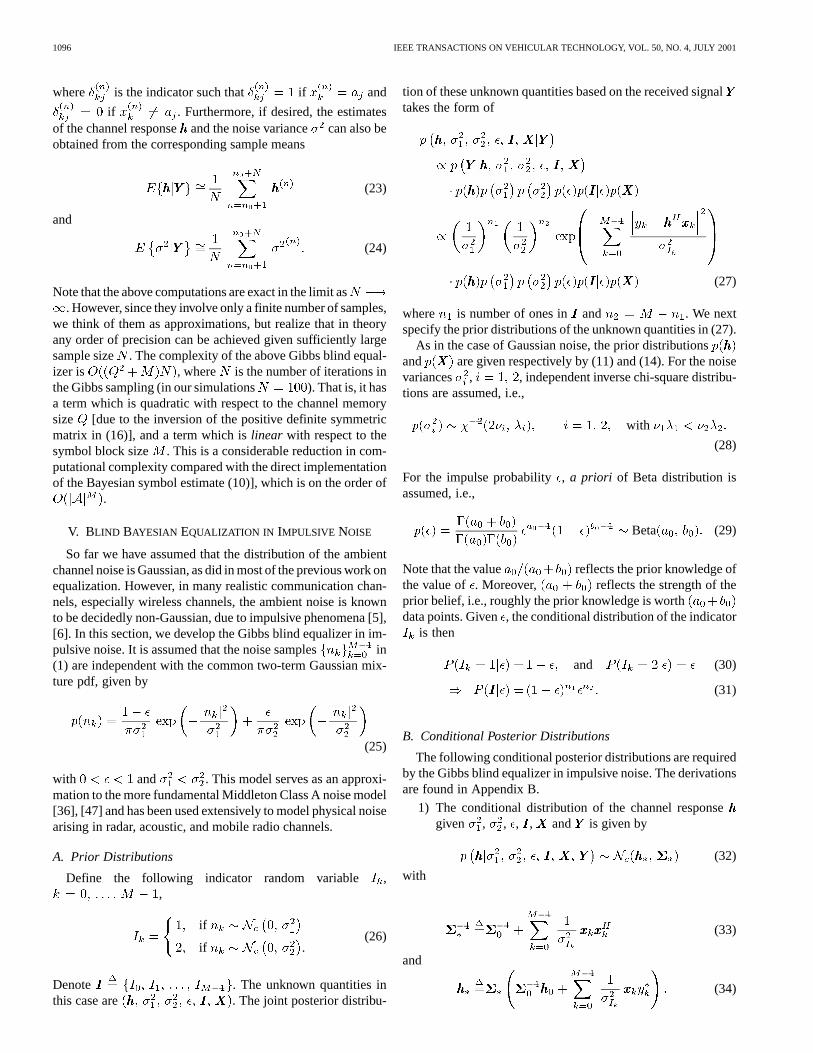
1096 IEEE TRANSACTIONS ON VEHICULAR TECHNOLOGY, VOL. 50, NO. 4, JULY 2001
where is the indicator such that if and
if . Furthermore, if desired, the estimatesof the channel responseand the noise variance can also beobtained from the corresponding sample means
(23)
and
(24)
Note that the above computations are exact in the limit as. However, since they involve only a finite number of samples,
we think of them as approximations, but realize that in theoryany order of precision can be achieved given sufficiently largesample size . The complexity of the above Gibbs blind equal-izer is , where is the number of iterations inthe Gibbs sampling (in our simulations ). That is, it hasa term which is quadratic with respect to the channel memorysize [due to the inversion of the positive definite symmetricmatrix in (16)], and a term which islinear with respect to thesymbol block size . This is a considerable reduction in com-putational complexity compared with the direct implementationof the Bayesian symbol estimate (10)], which is on the order of
.
V. BLIND BAYESIAN EQUALIZATION IN IMPULSIVE NOISE
So far we have assumed that the distribution of the ambientchannel noise is Gaussian, as did in most of the previous work onequalization. However, in many realistic communication chan-nels, especially wireless channels, the ambient noise is knownto be decidedly non-Gaussian, due to impulsive phenomena [5],[6]. In this section, we develop the Gibbs blind equalizer in im-pulsive noise. It is assumed that the noise samples in(1) are independent with the common two-term Gaussian mix-ture pdf, given by
(25)
with and . This model serves as an approxi-mation to the more fundamental Middleton Class A noise model[36], [47] and has been used extensively to model physical noisearising in radar, acoustic, and mobile radio channels.
A. Prior Distributions
Define the following indicator random variable ,,
if
if .(26)
Denote . The unknown quantities inthis case are . The joint posterior distribu-
tion of these unknown quantities based on the received signaltakes the form of
(27)
where is number of ones in and . We nextspecify the prior distributions of the unknown quantities in (27).
As in the case of Gaussian noise, the prior distributionsand are given respectively by (11) and (14). For the noisevariances , , independent inverse chi-square distribu-tions are assumed, i.e.,
with
(28)
For the impulse probability, a priori of Beta distribution isassumed, i.e.,
Beta (29)
Note that the value reflects the prior knowledge ofthe value of . Moreover, reflects the strength of theprior belief, i.e., roughly the prior knowledge is worthdata points. Given, the conditional distribution of the indicator
is then
and (30)
(31)
B. Conditional Posterior Distributions
The following conditional posterior distributions are requiredby the Gibbs blind equalizer in impulsive noise. The derivationsare found in Appendix B.
1) The conditional distribution of the channel responsegiven , , , , and is given by
(32)
with
(33)
and
(34)
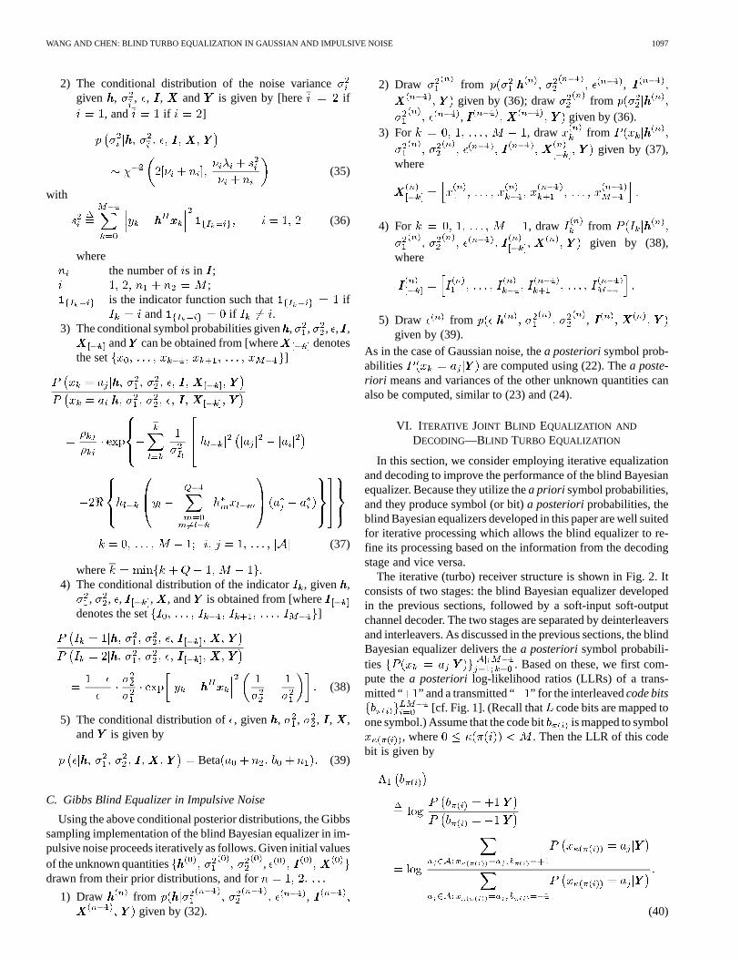
WANG AND CHEN: BLIND TURBO EQUALIZATION IN GAUSSIAN AND IMPULSIVE NOISE 1097
2) The conditional distribution of the noise variancegiven , , , , and is given by [here if
, and if ]
(35)
with
(36)
wherethe number of s in ;
;is the indicator function such that if
and if .3) The conditional symbol probabilities given, , , , ,
and can be obtained from [where denotesthe set ]
(37)
where .4) The conditional distribution of the indicator, given ,
, , , , , and is obtained from [wheredenotes the set ]
(38)
5) The conditional distribution of, given , , , , ,and is given by
Beta (39)
C. Gibbs Blind Equalizer in Impulsive Noise
Using the above conditional posterior distributions, the Gibbssampling implementation of the blind Bayesian equalizer in im-pulsive noise proceeds iteratively as follows. Given initial valuesof the unknown quantities ,drawn from their prior distributions, and for
1) Draw from ,given by (32).
2) Draw from ,given by (36); draw from, given by (36).
3) For , draw fromgiven by (37),
where
4) For , draw fromgiven by (38),
where
5) Draw from ,given by (39).
As in the case of Gaussian noise, thea posteriorisymbol prob-abilities are computed using (22). Thea poste-riori means and variances of the other unknown quantities canalso be computed, similar to (23) and (24).
VI. I TERATIVE JOINT BLIND EQUALIZATION AND
DECODING—BLIND TURBO EQUALIZATION
In this section, we consider employing iterative equalizationand decoding to improve the performance of the blind Bayesianequalizer. Because they utilize thea priori symbol probabilities,and they produce symbol (or bit)a posterioriprobabilities, theblind Bayesian equalizers developed in this paper are well suitedfor iterative processing which allows the blind equalizer to re-fine its processing based on the information from the decodingstage and vice versa.
The iterative (turbo) receiver structure is shown in Fig. 2. Itconsists of two stages: the blind Bayesian equalizer developedin the previous sections, followed by a soft-input soft-outputchannel decoder. The two stages are separated by deinterleaversand interleavers. As discussed in the previous sections, the blindBayesian equalizer delivers thea posteriorisymbol probabili-ties . Based on these, we first com-pute thea posteriori log-likelihood ratios (LLRs) of a trans-mitted “ ” and a transmitted “ ” for the interleavedcode bits
[cf. Fig. 1]. (Recall that code bits are mapped toone symbol.) Assume that the code bit is mapped to symbol
, where . Then the LLR of this codebit is given by
(40)
1098 IEEE TRANSACTIONS ON VEHICULAR TECHNOLOGY, VOL. 50, NO. 4, JULY 2001
Fig. 2. Iterative processing for joint blind Bayesian equalization and decoding—blind turbo equalizer.
Using the Bayes’ rule, (40) can be written as
(41)where the second term in (41), denoted by , representsthe a priori LLR of the code bit , which is computed bythe channel decoder in the previous iteration, interleaved andthen fed back to the blind Bayesian equalizer. (The superscript
indicates the quantity obtained from the previous iteration.)For the first iteration, assuming equally likely code bits, i.e., noprior information available, we then have , for
. The first term in (41), denoted by , rep-resents theextrinsicinformation delivered by the blind Bayesianequalizer based on the received signals, the structure of theISI-distorted signal given by (1), and the prior information aboutall other code bits. The extrinsic information , whichis not influenced by thea priori information providedby the channel decoder, is then reverse interleaved and fed intothe channel decoder as thea priori information in the next iter-ation.
Based on the extrinsic information of the code bits, and the structure of the channel code, the
soft-input soft-output channel decoder computes thea poste-riori LLR of each code bit
decoding
decoding
(42)
It is seen from (42) that the output of the soft-input soft-outputchannel decoder is the sum of the prior information ,and theextrinsic information delivered by the channeldecoder. This extrinsic information is the information about thecode bit gleaned from the prior information about the othercode bits, based on the constraint structure of thecode. The soft channel decoder also computes thea posterioriLLR of every information bit, which is used to make decisionon the decoded bit at the last iteration. After interleaving,the extrinsic information delivered by the channel decoder
is then used to compute thea priori symboldistributions defined in (6). Assume that a block ofbits
, , is mapped to symbol, for . Denote as the code bit index of
the th bit in the th symbol, where ,
and . The prior symbol probability is thengiven by
(43)
The code bit probabilities in (43) can be computed from thecorresponding LLRs as follows. Since
, after some manipulations we have for
(44)
The symbol probabilities are then fed back to theblind Bayesian equalizer as the prior information for the next it-eration. Note that at the first iteration, the extrinsic information
and are statistically independent. But subse-quently since they use the same information indirectly, they willbecome more and more correlated and finally the improvementthrough the iterations will diminish.
VII. D ISCUSSIONS
1) Shift and Phase Ambiguities:Blind deconvolutionproblem, in general, can only be solved up to a time-delayambiguity and sometimes also up to a phase ambiguity [2],[13], [32] if no further restrictions are imposed on the filtercoefficients . In particular, when forin (1), the time delay of the input signal is essentiallyunidentifiable. In fact, in this case, the models
, for are all practicallyequivalent to (1). As a result, the posterior distribution canbe an equally weighted mixture of several distributions, eachcorresponding to a particular time delay. In this case, estimatorsbased on the marginal distribution cannot be used. The globalMAP is a possible alternative, but it is difficult to obtain inhigh-dimensional cases. Furthermore, if the symbol alphabetis symmetric about zero, the blind equalizer is also subject toa phase ambiguity.

WANG AND CHEN: BLIND TURBO EQUALIZATION IN GAUSSIAN AND IMPULSIVE NOISE 1099
Fig. 3. Samples drawn by the blind Bayesian equalizer in a Gaussian ISI channel.E =N = 2 dB.
The phase ambiguity can be resolved by using differential en-coding and decoding [38]. The shift ambiguity can be resolvedif we impose constraints on the magnitudes of the channel taps,as will be discussed next. However, note that the use of differ-ential encoding/decoding makes the iterative joint equalizationand decoding scheme discussed in Section VI inapplicable. Thiscan be illustrated by the following simple example. Supposethat the code bit sequence is “000 000.” In differential encoding,let the first reference bit be “1.” Then the transmitted differen-tially encoded bit sequence becomes “1 111 111.” Now supposethat after channel decoding, the decoded code bit sequence is“010010,” i.e., decision errors are made on the second and thefifth bits. Then the differentially encoded bit sequence that isfed back to the equalizer (serving as the priors for the code bits)becomes “1 100 011.” That is, all the code bits between the twomistaken bits are erroneously encoded. Hence, differential en-coding can not be used in systems where the blind turbo equal-izer is employed as the receiver.
To resolve the delay and phase ambiguities, we adopt thecon-strainedGibbs sampler along the lines of [11], [12]. For ex-ample, we may impose constraints on the phase and amplitudeof a particular coefficient, say , e.g., , and
for some predetermined constantsand . To draw samples of that satisfy this condition, theso-calledrejection method[44] can be used. For instance, aftera sample is drawn from (15), check to see if the constraint is sat-isfied; if not, the sample is rejected and a new sample is drawnfrom (15); the procedure continues until a sample is obtainedthat satisfies the constraint. If a desired sample has not been ob-tained after a certain number of rejections, it is more appropriateto shift the s in the last sample until theth coefficient satis-
fies the constraint; the vacancies left at the end can be filled withzeros. Another plausible restriction on the amplitudes ofs isto specify the location of the largest one. For example, we mayrequire that for and some .
2) Initial Synchronization: In order to obtain the above-mentioned constraints on the channel coefficients, the receivermust be synchronized with the transmitter first. This can beaccomplished by transmitting a short knowncodedsequencefor sounding the channel. At the synchronization stage, uponreceiving the transmitted sounding signal, the blind Bayesianequalizer is employed to produce a possibly delayed and phaseshifted version of the transmitted symbol sequence. For eachpossible delay and phase shift, the corresponding code bitsequence is constructed and this sequence is passed through aViterbi decoder. Each decoded bit sequence is then comparedagainst the original sounding sequence. By locating the bestmatch we can identify the delay and phase ambiguities.
3) Decoder-Assisted Convergence Assessment:Detectingconvergence in the Gibbs sampler is usually done in anadhoc way. Some methods can be found in [41]. One of themis to monitor a sequence of weights that measure the discrep-ancy between the sampled and the desired distribution. Inthe application considered here, since the blind equalizer isfollowed by a channel decoder, we can assess convergence bymonitoring the number of bit corrections made by the channeldecoder. If this number exceeds some predetermined threshold,then we decide convergence is not achieved. In that case theGibbs blind equalizer will be applied again to the same datablock. The rationale is that if the Gibbs sampler has reachedconvergence, then the symbol (and bit) errors after equalizationshould be relatively small. On the other hand, if convergence
1100 IEEE TRANSACTIONS ON VEHICULAR TECHNOLOGY, VOL. 50, NO. 4, JULY 2001
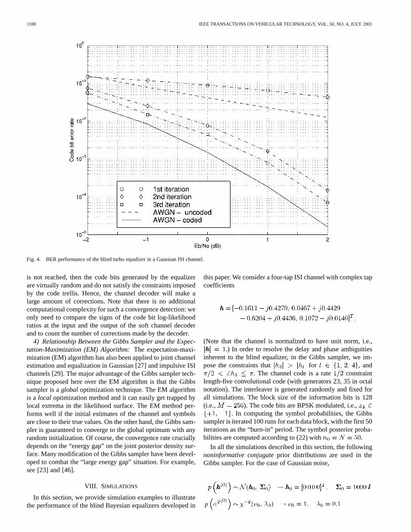
Fig. 4. BER performance of the blind turbo equalizer in a Gaussian ISI channel.
is not reached, then the code bits generated by the equalizerare virtually random and do not satisfy the constraints imposedby the code trellis. Hence, the channel decoder will make alarge amount of corrections. Note that there is no additionalcomputational complexity for such a convergence detection: weonly need to compare the signs of the code bit log-likelihoodratios at the input and the output of the soft channel decoderand to count the number of corrections made by the decoder.
4) Relationship Between the Gibbs Sampler and the Expec-tation-Maximization (EM) Algorithm:The expectation-maxi-mization (EM) algorithm has also been applied to joint channelestimation and equalization in Gaussian [27] and impulsive ISIchannels [29]. The major advantage of the Gibbs sampler tech-nique proposed here over the EM algorithm is that the Gibbssampler is aglobal optimization technique. The EM algorithmis a local optimization method and it can easily get trapped bylocal extrema in the likelihood surface. The EM method per-forms well if the initial estimates of the channel and symbolsare close to their true values. On the other hand, the Gibbs sam-pler is guaranteed to converge to the global optimum with anyrandom initialization. Of course, the convergence rate cruciallydepends on the “energy gap” on the joint posterior density sur-face. Many modification of the Gibbs sampler have been devel-oped to combat the “large energy gap” situation. For example,see [23] and [46].
VIII. SIMULATIONS
In this section, we provide simulation examples to illustratethe performance of the blind Bayesian equalizers developed in
this paper. We consider a four-tap ISI channel with complex tapcoefficients
(Note that the channel is normalized to have unit norm, i.e.,.) In order to resolve the delay and phase ambiguities
inherent to the blind equalizer, in the Gibbs sampler, we im-pose the constraints that for , and
. The channel code is a rate constraintlength-five convolutional code (with generators 23, 35 in octalnotation). The interleaver is generated randomly and fixed forall simulations. The block size of the information bits is 128(i.e., ). The code bits are BPSK modulated, i.e.,
. In computing the symbol probabilities, the Gibbssampler is iterated 100 runs for each data block, with the first 50iterations as the “burn-in” period. The symbol posterior proba-bilities are computed according to (22) with .
In all the simulations described in this section, the followingnoninformative conjugateprior distributions are used in theGibbs sampler. For the case of Gaussian noise,
WANG AND CHEN: BLIND TURBO EQUALIZATION IN GAUSSIAN AND IMPULSIVE NOISE 1101
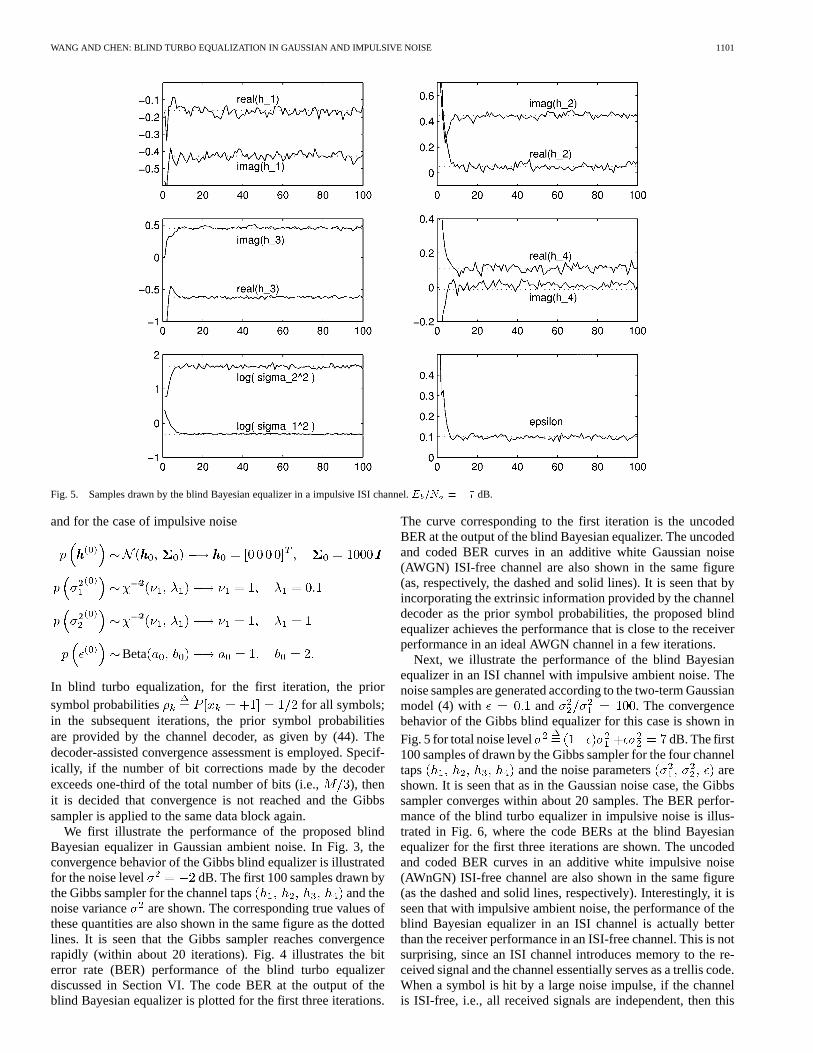
Fig. 5. Samples drawn by the blind Bayesian equalizer in a impulsive ISI channel.E =N = �7 dB.
and for the case of impulsive noise
Beta
In blind turbo equalization, for the first iteration, the priorsymbol probabilities for all symbols;in the subsequent iterations, the prior symbol probabilitiesare provided by the channel decoder, as given by (44). Thedecoder-assisted convergence assessment is employed. Specif-ically, if the number of bit corrections made by the decoderexceeds one-third of the total number of bits (i.e., ), thenit is decided that convergence is not reached and the Gibbssampler is applied to the same data block again.
We first illustrate the performance of the proposed blindBayesian equalizer in Gaussian ambient noise. In Fig. 3, theconvergence behavior of the Gibbs blind equalizer is illustratedfor the noise level dB. The first 100 samples drawn bythe Gibbs sampler for the channel taps and thenoise variance are shown. The corresponding true values ofthese quantities are also shown in the same figure as the dottedlines. It is seen that the Gibbs sampler reaches convergencerapidly (within about 20 iterations). Fig. 4 illustrates the biterror rate (BER) performance of the blind turbo equalizerdiscussed in Section VI. The code BER at the output of theblind Bayesian equalizer is plotted for the first three iterations.
The curve corresponding to the first iteration is the uncodedBER at the output of the blind Bayesian equalizer. The uncodedand coded BER curves in an additive white Gaussian noise(AWGN) ISI-free channel are also shown in the same figure(as, respectively, the dashed and solid lines). It is seen that byincorporating the extrinsic information provided by the channeldecoder as the prior symbol probabilities, the proposed blindequalizer achieves the performance that is close to the receiverperformance in an ideal AWGN channel in a few iterations.
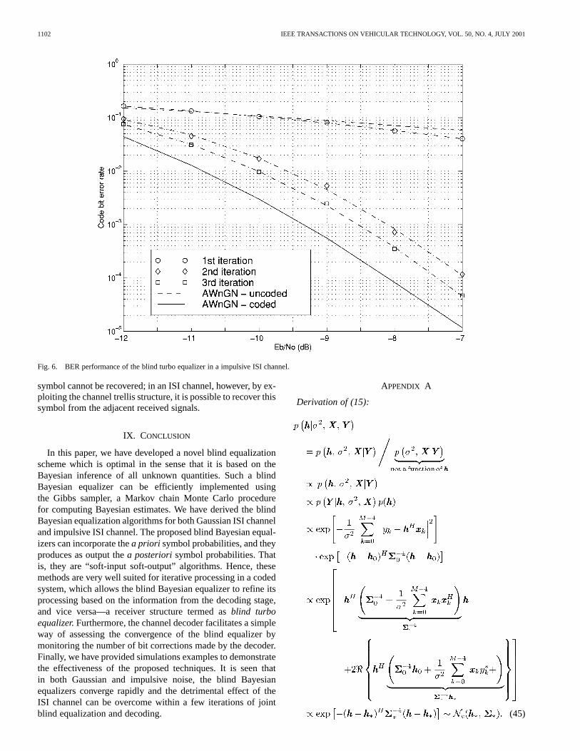
Next, we illustrate the performance of the blind Bayesianequalizer in an ISI channel with impulsive ambient noise. Thenoise samples are generated according to the two-term Gaussianmodel (4) with and . The convergencebehavior of the Gibbs blind equalizer for this case is shown inFig. 5 for total noise level dB. The first100 samples of drawn by the Gibbs sampler for the four channeltaps and the noise parameters areshown. It is seen that as in the Gaussian noise case, the Gibbssampler converges within about 20 samples. The BER perfor-mance of the blind turbo equalizer in impulsive noise is illus-trated in Fig. 6, where the code BERs at the blind Bayesianequalizer for the first three iterations are shown. The uncodedand coded BER curves in an additive white impulsive noise(AWnGN) ISI-free channel are also shown in the same figure(as the dashed and solid lines, respectively). Interestingly, it isseen that with impulsive ambient noise, the performance of theblind Bayesian equalizer in an ISI channel is actually betterthan the receiver performance in an ISI-free channel. This is notsurprising, since an ISI channel introduces memory to the re-ceived signal and the channel essentially serves as a trellis code.When a symbol is hit by a large noise impulse, if the channelis ISI-free, i.e., all received signals are independent, then this
1102 IEEE TRANSACTIONS ON VEHICULAR TECHNOLOGY, VOL. 50, NO. 4, JULY 2001
Fig. 6. BER performance of the blind turbo equalizer in a impulsive ISI channel.
symbol cannot be recovered; in an ISI channel, however, by ex-ploiting the channel trellis structure, it is possible to recover thissymbol from the adjacent received signals.
IX. CONCLUSION
In this paper, we have developed a novel blind equalizationscheme which is optimal in the sense that it is based on theBayesian inference of all unknown quantities. Such a blindBayesian equalizer can be efficiently implemented usingthe Gibbs sampler, a Markov chain Monte Carlo procedurefor computing Bayesian estimates. We have derived the blindBayesian equalization algorithms for both Gaussian ISI channeland impulsive ISI channel. The proposed blind Bayesian equal-izers can incorporate thea priori symbol probabilities, and theyproduces as output thea posteriorisymbol probabilities. Thatis, they are “soft-input soft-output” algorithms. Hence, thesemethods are very well suited for iterative processing in a codedsystem, which allows the blind Bayesian equalizer to refine itsprocessing based on the information from the decoding stage,and vice versa—a receiver structure termed asblind turboequalizer.Furthermore, the channel decoder facilitates a simpleway of assessing the convergence of the blind equalizer bymonitoring the number of bit corrections made by the decoder.Finally, we have provided simulations examples to demonstratethe effectiveness of the proposed techniques. It is seen thatin both Gaussian and impulsive noise, the blind Bayesianequalizers converge rapidly and the detrimental effect of theISI channel can be overcome within a few iterations of jointblind equalization and decoding.
APPENDIX A
Derivation of (15):
(45)
WANG AND CHEN: BLIND TURBO EQUALIZATION IN GAUSSIAN AND IMPULSIVE NOISE 1103
Derivation of (18):
(46)
Derivation of (20):
where (47)
(48)
APPENDIX B
Derivation of (32):
(49)
Derivation of (36):
1104 IEEE TRANSACTIONS ON VEHICULAR TECHNOLOGY, VOL. 50, NO. 4, JULY 2001
(50)
Derivation of (37):
(51)
(52)
Derivation of (38):
(53)
(54)
Derivation of (39):
Beta (55)
REFERENCES
[1] K. Abend and B. D. Fritchman, “Statistical detection for communica-tion channels with intersymbol interference,”Proc. IEEE, vol. 58, pp.779–785, May 1970.
[2] A. Benveniste, M. Goursat, and G. Ruget, “Robust identification of anonminimum phase system: Blind adjustment of a linear equalizer indata communications,”IEEE Trans. Automat. Contr., vol. AC-25, pp.385–399, June 1980.
[3] C. Berrou and A. Glavieux, “Near optimum error-correcting coding anddecoding: Turbo codes,”IEEE Trans. Commun., vol. 44, Oct. 1996.
[4] C. Berrou, A. Glavieux, and P. Thitimajshima, “Near Shannon limiterror-correction coding and decoding: Turbo codes,” inProc. 1993 Int.Conf. Communications (ICC’93), Geneva, Switzerland, June 1993, pp.1064–1070.
[5] K. L. Blackard, T. S. Rappaport, and C. W. Bostian, “Measurements andmodels of radio frequency impulsive noise for indoor wireless commu-nications,”IEEE J. Select. Areas Commun., vol. 11, pp. 991–1001, Sept.1993.
[6] T. K. Blankenship, D. M. Krizman, and T. S. Rappaport, “Measure-ments and simulation of radio frequency impulsive noise in hospitalsand clinics,” inProc. 1997 IEEE Vehicular Technology Conf. (VTC’97),Phoenix, AZ, May 1997, pp. 1942–1946.
[7] G. E. Box and G. C. Tiao,Bayesian Inference in Statistical Anal-ysis. Reading, MA: Addison-Wesley, 1973.
[8] P. L. Brockett, M. Hinich, and G. R. Wilson, “Nonlinear andnon-Gaussian ocean noise,”J. Acoust. Soc. Amer., vol. 82, pp.1286–1399, 1987.
[9] I. Cha and S. A. Saleem, “Non-linear filtering and equalization in non-Gaussian noise using radial basis function and related networks,” inProc. 31st Annu. Asilomar Conf. Signals, Systems, and Computers, Pa-cific Grove, CA, Nov. 1997, pp. 13–17.
[10] K. S. Chan, “Asymptotic behavior of the Gibbs sampler,”J. Amer. Stat.Assoc., vol. 88, pp. 320–326, 1993.
[11] R. Chen and T. H. Li, “Blind restoration of linearly degraded discretesignals by Gibbs sampling,”IEEE Trans. Signal Processing, vol. 10, pp.2410–2413, Oct. 1995.
[12] R. Chen and J. S. Liu, “Predictive updating methods with applications toBayesian classification,”J. Royal Statist. Soc. B, vol. 58, pp. 397–415,1995.
[13] K. Dogancay and R. A. Kennedy, “Blind detection of equalization errorsin communication systems,”IEEE Trans. Inform. Theory, vol. 43, pp.469–482, Mar. 1997.
[14] C. Douillard, M. Jezequel, C. Berrou, A. Picart, P. Didier, and A. Gle-vieux, “Iterative correction of intersymbol interference: Turbo equaliza-tion,” Eur. Trans. Telecommun., vol. 6, no. 5, pp. 507–511, Sept.–Oct.1995.
[15] S. Haykin, Ed.,Blind Deconvolution. Englewood Cliffs, NJ: Prentice-Hall, 1994.
WANG AND CHEN: BLIND TURBO EQUALIZATION IN GAUSSIAN AND IMPULSIVE NOISE 1105
[16] C. R. Johnsonet al., “Blind equalization using the constant moduluscriterion: A review,”Proc. IEEE, vol. 86, pp. 1927–1950, Oct. 1998.
[17] M. Feder and A. Catipovic, “Algorithms for joint channel estimation anddata recovery—Application to equalization in underwater communica-tions,” IEEE J. Oceanic Eng., vol. 16, pp. 42–55, Jan. 1991.
[18] A. E. Gelfand and A. F. W. Smith, “Sampling-based approaches to cal-culating marginal densities,”J. Amer. Stat. Assoc., vol. 85, pp. 398–409,1990.
[19] A. Gelman, J. B. Carlin, H. S. Stern, and D. B. Rubin,Bayesian DataAnalysis. London, U.K.: Chapman Hall, 1995.
[20] S. Geman and D. Geman, “Stochastic relaxation, Gibbs distribution, andthe Bayesian restoration of images,”IEEE Trans. Pattern Anal. MachineIntell., vol. PAMI-6, pp. 721–741, Nov. 1984.
[21] M. Ghosh and C. L. Weber, “Maximum likelihood blind equalization,”Opt. Eng., vol. 31, pp. 1224–1228, June 1992.
[22] K. Giridhar, J. J. Shynk, and R. A. Iltis, “Bayesian/decision-feedbackalgorithm for blind equalization,”Opt. Eng., vol. 31, pp. 1211–1223,June 1992.
[23] P. J. Green, “Revisible jump Markov chain Monte Carlo computationand Bayesian model determination,”Biometrika, vol. 82, pp. 711–732,1985.
[24] J. Hagenauer, “The Turbo principle: Tutorial introduction and state of theart,” in Proc. Int. Symp. Turbo Codes and Related Topics, Brest, France,Sept. 1997, pp. 1–11.
[25] R. A. Iltis, “A Bayesian maximum-likelihood sequence estimation algo-rithm fora priori unknown channels and symbol timing,”IEEE J. Select.Areas Commun., vol. 10, pp. 579–588, Apr. 1992.
[26] R. A. Iltis, J. J. Shynk, and K. Giridhar, “Bayesian algorithms for blindequalization using parallel adaptive filters,”IEEE Trans. Commun., vol.42, pp. 1017–1032, Mar. 1994.
[27] G. K. Kaleh and R. Vallet, “Joint parameter estimation and symbol detec-tion for linear or nonlinear unknown channels,”IEEE Trans. Commun.,vol. 42, pp. 2406–2413, July 1994.
[28] S. A. Kassam and H. V. Poor, “Robust techniques for signal processing:A survey,”Proc. IEEE, vol. 73, pp. 433–481, Mar. 1985.
[29] R. J. Kozick, R. S. Blum, and B. M. Sadler, “Signal processing in non-Gaussian noise using mixture distribution and the EM algorithm,” inProc. 31st Annu. Asilomar Conf. Signals, Systems, and Computers, Pa-cific Grove, CA, Nov. 1997, pp. 438–442.
[30] G.-K. Lee, S. B. Gelfand, and M. P. Fitz, “Bayesian techniques for blinddeconvolution,”IEEE Trans. Commun., vol. 44, pp. 826–835, July 1996.
[31] E. L. Lehmann and G. Casella,Theory of Point Estimation, 2 ed. NewYork: Springer-Verlag, 1998.
[32] K. S. Lii and M. Rosenblatt, “Deconvolution and estimation of transferfunction phase and coefficients for non-Gaussian linear process,”Ann.Statistics, vol. 10, pp. 1195–1208, 1982.
[33] J. S. Liu, A. Kong, and W. H. Wong, “Covariance structure of the Gibbssampler with applications to the comparisons of estimators and augmen-tation schemes.,”Biometrika, vol. 81, pp. 27–40, 1994.
[34] D. Middleton, “Man-made noise in urban environments and transporta-tion systems: Models and measurement,”IEEE Trans. Commun., vol.COM-21, pp. 1232–1241, Nov. 1973.
[35] , “Statistical-physical models of electromagnetic interference,”IEEE Trans. Electromagn. Compat., vol. EMC-19, pp. 106–127, 1977.
[36] , “Channel modeling and threshold signal processing in underwateracoustics: An analytical overview,”IEEE J. Oceanic Eng., vol. OE-12,pp. 4–28, 1987.
[37] D. Middleton and A. D. Spaulding, “Elements of weak signal detectionin non-Gaussian noise,” inAdvances in Statistical Signal Processing Vol.2: Signal Detection, H. V. Poor and J. B. Thomas, Eds. Greenwich, CT:JAI, 1993.
[38] J. G. Proakis,Digital Communications, 3 ed. New York: McGraw-Hill, 1995.
[39] M. J. Schervish and B. P. Carlin, “On the convergence of successive sub-stitution sampling,”J. Computat. Graphical Statist., vol. 1, pp. 111–127,1992.
[40] N. Seshadri, “Joint channel and data estimation using blind trellissearch techniques,”IEEE Trans. Commun., vol. 42, pp. 1000–1016,Feb./Mar./Apr. 1994.
[41] M. A. Tanner, Tools for Statistics Inference. New York:Springer-Verlag, 1991.
[42] M. A. Tanner and W. H. Wong, “The calculation of posterior distributionby data augmentation (with discussion),”J. Amer. Statist. Assoc., vol. 82,pp. 528–550, 1987.
[43] L. Tong and S. Perreau, “Multichannel blind identification and equal-ization based on second-order statistics: From subspace to maximumlikelihood methods,”Proc. IEEE, vol. 86, Oct. 1998.
[44] J. von Neumann, “Various techniques used in connection with randomdigit,” Nat. Bureau Standards Appl. Math. Ser., vol. 12, pp. 36–38, 1951.
[45] X. Wang and H. V. Poor, “Iterative (Turbo) soft interference cancellationand decoding for coded CDMA,”IEEE Trans. Commun., vol. 47, July1999.
[46] W. H. Wong and F. Liang, “Dynamic importance weighting inMonte Carlo and optimization,”Proc. Nat. Acad. Sci., vol. 94, pp.14220–14 224, 1997.
[47] S. M. Zabin and H. V. Poor, “Efficient estimation of the class A param-eters via the EM algorithm,”IEEE Trans. Inform., vol. 37, pp. 60–72,Jan 1991.
Xiaodong Wang (M’00) received the B.S. degreein electrical engineering and applied mathematics(highest honor) from Shanghai Jiao Tong University,Shanghai, China, in 1992, the M.S. degree inelectrical and computer engineering from PurdueUniversity, West Lafayette, IN, in 1995, andthe Ph.D. degree in electrical engineering fromPrinceton University, Princeton, NJ, in 1998.
In July 1998, he joined the Department of Elec-trical Engineering, Texas A&M University, CollegeStation, as an Assistant Professor. He has worked in
the areas of digital communications, digital signal processing, parallel and dis-tributed computing, nanoelectronics, and quantum computing. He was with theAT&T Research Laboratories, Red Bank, NJ, during the summer of 1997. Hisresearch interests fall in the general areas of computing, signal processing, andcommunications. Currently, his research interests include multi-user communi-cations theory and advanced signal processing for wireless communications.
Dr. Wang is a member of the American Association for the Advancement ofScience. He received the 1999 NSF CAREER Award.
Rong Chenreceived the B.S. degree in mathematicsfrom Peking University, Beijing, China, in 1985and the M.S. and Ph.D. degrees in statistics fromCarnegie Mellon University, Pittsburgh, PA, in 1987and 1990, respectively.
From September 1990 to May 1999, he was withthe Department of Statistics, Texas A&M University,College Station, first as an Assistant Professor andthen as an Associate Professor. He is now a Professorof statistics in the Department of Information andDecision Sciences, University of Illinois at Chicago.
His current research interests include nonlinear/nonparametric time series andMonte Carlo methods for nonlinear non-Gaussian dynamic systems.
Dr. Chen is a member of the American Statistical Association and the Instituteof Mathematical Statistics.


![[Murrey Jeneth] Impulsive Proposal](https://img.pdfslide.net/doc/110x75/563db8ff550346aa9a99002a/murrey-jeneth-impulsive-proposal.jpg)