Blur clariﬁed: A review and synthesis of blur discrimination

Blur clarified: A review and synthesisof blur discrimination

NASA Ames Research Center, Moffett Field, CA, USAAndrew B. Watson

NASA Ames Research Center, Moffett Field, CA, USAAlbert J. Ahumada

Blur is an important attribute of human spatial vision, and sensitivity to blur has been the subject of considerableexperimental research and theoretical modeling. Often, these models have invoked specialized concepts or mechanisms,such as intrinsic blur, multiple spatial frequency channels, or blur estimation units. In this paper, we review the severalexperimental studies of blur discrimination and find that they are in broad empirical agreement. However, contrary toprevious modeling efforts, we find that specialized mechanisms are not required and that the essential features of blurdiscrimination are fully accounted for by a visible contrast energy (ViCE) model, in which two spatial patterns aredistinguished when the integrated difference between their masked local visible contrast energy responses reaches athreshold value. In the ViCE model, intrinsic blur is represented by the high-frequency limb of the contrast sensitivityfunction, but the low-frequency limb also contributes to the predictions for large reference blurs, and the model includesmasking, which improves predictions for high-contrast stimuli.

Keywords: computational modeling, contrast sensitivity, detection/discrimination, masking, spatial vision

Citation: Watson, A. B., & Ahumada, A. J. (2011). Blur clarified: A review and synthesis of blur discrimination. Journal ofVision, 11(5):10, 1–23, http://www.journalofvision.org/content/11/5/10, doi:10.1167/11.5.10.

Introduction

Like many terms that we take for granted, blur issurprisingly difficult to define. Dictionaries typically statethat to blur is to render indistinct, usually by smudging orsmearing, but sometimes by dimming, or through obscu-ration by fog, by soot, or by a blow to the head. In thenarrower technical context of vision, optics, and imaging,blurring generally connotes a smearing of an image,through some amount of low-pass filtering.In this sense, all optical systems, and indeed all imaging

systems, exhibit some blur. Over the last six decades, ithas become commonplace to analyze the early parts of thevisual system as an imaging system, incorporating variousoptical and neural filtering operations. This in turn has ledto questions about blur in vision: its nature, its magnitude,and its effect on visual tasks such as detection, recog-nition, and localization (Chen, Chen, Tseng, Kuo, &Wu, 2009; Hamerly &Dvorak, 1981; Hess, Pointer, &Watt,1989; Mather & Smith, 2002; Paakkonen & Morgan,1994; Watt & Morgan, 1983; Westheimer, Brincat, &Wehrhahn, 1999; Wuerger, Owens, & Westland, 2001).Most of these studies have employed Gaussian blur,defined as convolution with a Gaussian impulse response.The study of blur may also be connected to recent

studies on wavefront aberrations of the eye, which haveled to ever more detailed descriptions of the opticaltransfer function of the visual system (Thibos, Hong,Bradley, & Cheng, 2002) and to theoretical connectionsbetween optical blur and basic functions of detection,

discrimination, and acuity (Thibos, 2009; Watson &Ahumada, 2008). These studies generalize the concept ofblur beyond Gaussian blur to more complex and realisticoptical blurring functions. Optical blur usually differsfrom Gaussian blur. When higher order aberrations areincluded, the optical point spread function can be quitecomplex. When only diffraction and defocus are consid-ered, the point spread is simpler but still differs from aGaussian.There has also been interest in the role of blur as a

visual cue. Optical blur is a powerful cue to accommoda-tion, since it will generally be minimized when the eye isaccommodated at near the depth of the viewed object(Kruger & Pola, 1986). Likewise, since blur will increaseat larger or smaller depths, blur contributes to the sense ofdepth (Held, Cooper, O’Brien, & Banks, 2010; Mather &Smith, 2002). Motion of an object relative to the observerwill also blur the image of the object by an amount and ina manner that is characteristic of the object’s velocity.This has led to theories of visual motion estimation fromblur (Barlow & Olshausen, 2004; Burr & Ross, 2002;Geisler, 1999; Harrington & Harrington, 1981).Because of its role in driving accommodation, there has

been significant work on human sensitivity to opticalblur (Campbell & Westheimer, 1958; Legras, Chateau, &Charman, 2004; Walsh & Charman, 1988; Wang &Ciuffreda, 2005). In a particularly elegant early study,Campbell and Westheimer (1958) measured the thresholdamplitude for modulations of defocus around some fixedvalue and found that the minimum (È0.2 D) correspondedto the previously measured amplitude of normal fluctuations

Journal of Vision (2011) 11(5):10, 1–23 http://www.journalofvision.org/content/11/5/10 1

doi: 10 .1167 /11 .5 .10 Received March 28, 2011; published September 15, 2011 ISSN 1534-7362 * ARVO

http://vision.arc.nasa.gov/

http://vision.arc.nasa.gov/

mailto:[email protected]?subject=http://www.journalofvision.org/content/11/5/10


http://vision.arc.nasa.gov/personnel/al/ahumada.html

http://vision.arc.nasa.gov/personnel/al/ahumada.html



http://www.journalofvision.org/content/11/5/10

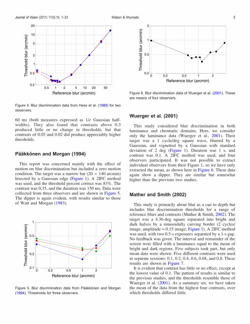
in accommodation. Most relevant to the present review,their data are the first published instance of a “dipper,” inwhich the minimum threshold is found for fluctuationsaround a fixed amount of defocus greater than zero. Thisdipper for optical blur was confirmed under a wide varietyof conditions by later studies (Walsh & Charman, 1988).We do not analyze these studies in detail here but notethat their results should be addressed by any general blurdiscrimination model.In the context of visual displays, there is an applied

interest in human sensitivity to blur. Many displayattributes, such as resolution, pixel shape (Farrell, Xu,Larson, & Wandell, 2009), surface coatings, screen grain(Fiske, Silverstein, Hodgson, & Watson, 2007), andmotion blur (Watson, 2010a, 2010b) will affect theamount of rendered image blur. It is essential to under-stand human sensitivity to blur in order to optimize theengineering and economic trade-offs in design of thesedisplays. Blur has also long been a central concern inautomated analysis of image quality (Granger & Cupery,1972). For image processing operations such as scaling,compression, or enhancement, it is important to knowwhether perceptible blur has been introduced. In fact,among the earliest direct measurements of blur detectionand discrimination were those made as part of an appliedinterest in image sharpness (Hamerly & Dvorak, 1981).Since that time, many “blur metrics” have been devised toassess the sharpness of images (Ferzli & Karam, 2006;Kayargadde & Martens, 1996).One approach to the study of human perception of blur

is to ask observers to make judgments of photographicimages subjected to blurring or sharpening operations(de Ridder, 2001b; Field & Brady, 1997; Parraga,Troscianko, & Tolhurst, 2005; Tadmor & Tolhurst,1994). However, this has not led to simple models, perhapsbecause the statistics of natural images are not stationaryor because suprathreshold blur estimates are subject tocontext effects (de Ridder, 2001a). Indeed, it has beenshown that sharpness or blur estimates can be stronglymanipulated by adaptation to blurred or sharpened images(Elliott, Georgeson, & Webster, 2011; Webster, 2011;Webster, Georgeson, & Webster, 2002).Alternatively, one can study the perception of blur in a

single edge. An edge is a transition between two differentluminances. When the edge is straight, there is novariation in the dimension orthogonal to the edge, andwe can consider just the one-dimensional cross section ofthe edge. In the limiting case of an edge with no blur, thetransition is a step function. An edge may be blurred byconvolving it with a blurring kernel. In the experimentsdiscussed here, this is typically a Gaussian with unit area.The width of the Gaussian, usually characterized by itsstandard deviation, is a measure of the amount of blur.In one classic experimental design, an observer is

presented with a pair of edges, identical except for theirrespective blurs. One is said to have the “reference” blur

and the other a larger “test” blur, which may beconsidered the reference plus an added blur. The observeris asked to identify the edge with the larger blur. Over aseries of trials, the reference blur is fixed, while theamount of added blur is varied, so as to determine thethreshold blur increment, that is, the amount of added blurat which the observer is correct some specified percentageof the time. When the reference blur is zero (step edge vs.blurred edge), this threshold is the absolute threshold forblur detection. When the reference blur is greater thanzero, the measurement is of blur discrimination. Thismeasurement is repeated for a number of values of thereference blur to produce an empirical function that wewill call the threshold vs. reference (TVR) curve.A number of models and theories have been constructed

to explain the results of blur discrimination experiments ofthis sort. These theories have often assumed explicitestimation of blur magnitude (Watt, 1988) and have ofteninvoked ad hoc concepts such as “intrinsic blur” (Mather& Smith, 2002; Paakkonen & Morgan, 1994; Watt, 1988).Likewise, they have often attributed the form of the TVRcurve to interaction among multiple channels (Hess et al.,1989; Watt & Morgan, 1984) or complex nonlinearcontrast normalization schemes (Chen et al., 2009). Theseideas will be discussed in more detail below.The first purpose of this report is to review the several

studies that have analyzed blur detection and discrim-ination in this manner. Despite many differences in stimuliand procedures, the various studies will be shown tolargely agree on the basic pattern of results. The secondpurpose is to review briefly the various theories that havebeen put forward to account for the data. The third andfinal goal will be to show that a simple model of visiblecontrast energy detection can account for the essentials ofthe data and that, consequently, no additional mechanismsor models are required.

Data

We consider here the data extracted from eight studiesof blur detection and discrimination. While varying inmany details, all employed a similar paradigm. In eachstudy, an observer attempted to discriminate between twostimuli, one containing an edge (or edges) with somereference amount of blur and the other identical except fora larger test blur. Threshold is quantified as the differencebetween reference and test amounts of blur at somespecified percent correct.In the following sections, we describe briefly the

stimuli, methods, and data from each study. The studies arepresented in chronological order, except for Westheimeret al. (1999), in which only blur detection thresholds weremeasured. Data were extracted from published figuresusing manual location of points in the graphic and

Journal of Vision (2011) 11(5):10, 1–23 Watson & Ahumada 2

subsequent processing of locations by software of ourdesign. To compare these diverse sets of data, it isnecessary to adopt consistent notation and plottingconventions. Here, all blur measurements are expressedas the standard deviation of a Gaussian, in minutes of arcof visual angle (arcmin). Where the actual blur was otherthan Gaussian, such as a ramp or cosine, it has beenconverted to the closest Gaussian in a mean square errorsense. Our standard plot is what we call the thresholdversus reference (TVR) curve, that is, the threshold blurincrement as a function of the reference blur. Threshold isdefined as the blur increment that yields a fixed percentcorrect. Unless otherwise stated, this percentage was 75%;in some cases, values up to 83% were used. In most plots,threshold and reference axes are logarithmic and areequally scaled. Where present, points with a zero abscissa(zero reference blur) are plotted at 0.1 or lower, with abroken x-axis. Where possible, a consistent color code isused to identify each study. From each study, we have

derived a summary curve by averaging over observers orconditions, as described in the text. These summaries willease comparison of data and models.In Figure 1, we show our reconstructions of the stimuli

used in these eight studies. To allow comparisons, theimages are all drawn to a common scale. In each study,we embed the stimulus in a 0.25-deg-wide margin of thebackground luminance. In many cases, there were ambi-guities regarding stimulus details (e.g., luminance of thebackground), and in those cases, we have made our bestinference. In all cases, we have contacted the authors toconfirm general accuracy. Further details on these stimuliwill be provided in the following sections.To provide the reader with additional insight, we have

provided an animated demonstration of a blur discrim-ination task. This demonstration allows the reader toadjust the stimulus parameters and perform their own blurdiscrimination judgments. This demonstration, along withthree others, require the use of a free browser plug-in.

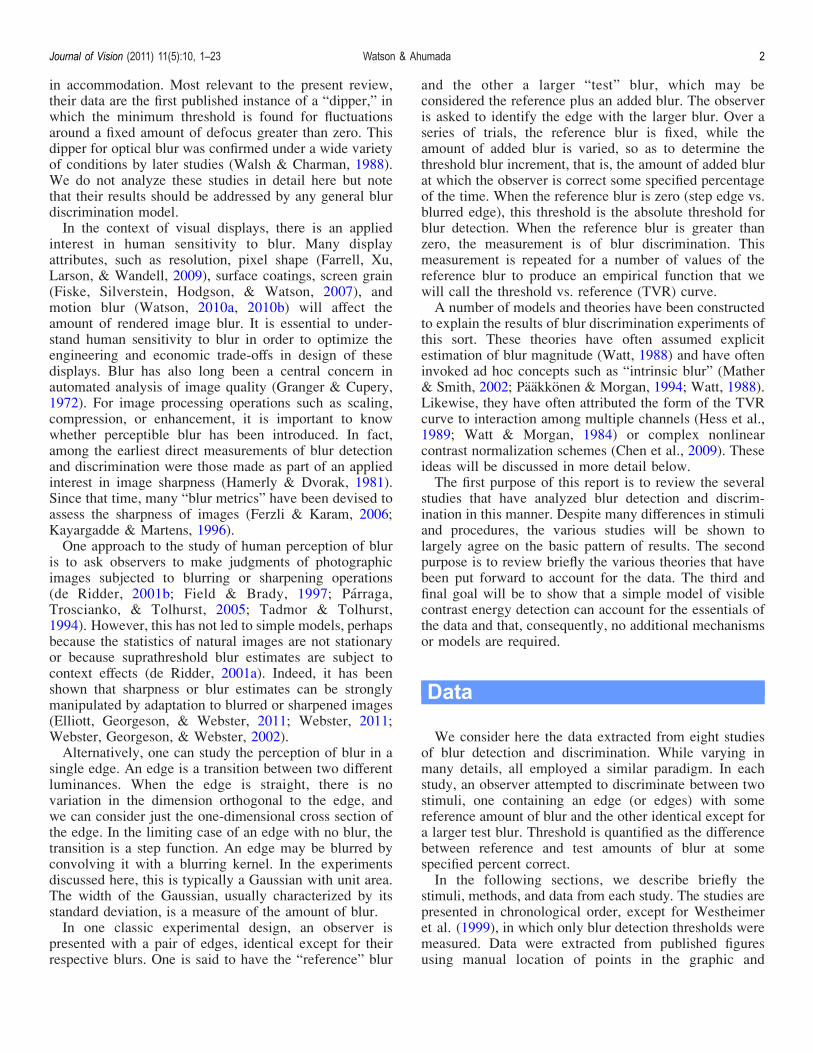
Figure 1. Stimuli used in eight studies of blur detection and discrimination. All stimuli are drawn to scale. Each stimulus is surrounded by a0.25-deg-wide margin of our estimate of the background. In each stimulus, the blur width (standard deviation) is 4 arcmin.


http://www.journalofvision.org/site/misc/cdf/watson-jov-blur-demos.xhtml

Hamerly and Dvorak (1981)

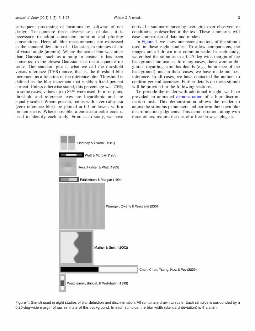
In this early paper, the authors used a pair of edges,aligned and separated by 12 arcmin (Figure 1). Twoobservers (the authors) and two contrasts (0.333 and0.818) were used. A 2AFC method was used, andinspection time was unspecified and thus assumed to beunlimited. Data are shown in Figure 2. Because differentreference blur sets were used for the two observers, wehave created a mean set by averaging linear interpolationsof each observer’s mean, sampled at the union of allreference blurs used. This is shown by the gray points inFigure 2.The data show a clear decline in threshold with

increasing reference blur. This is the beginning of theso-called “dipper” shape, though the study does not usereference blurs large enough to show the subsequent rise.As will be noted below, the mean thresholds are 2 to 5 timeslower than estimates from the other studies consideredhere.Contrast has a very small effect for one observer and,

essentially, no effect for the other. The two observersdiffer by, on average, a factor of 2.6. As will be notedbelow, these thresholds are well below those measured inother studies. They also explore a much smaller range ofreference blur. As a summary set, we have taken the meanof all four data sets.

Watt and Morgan (1983)

These authors used a narrow bar (180 � 12 arcmin)containing two edges separated by 90 arcmin (Figure 1).The background luminance outside the stimulus was notspecified but was dark, since a calligraphic display wasused (a cathode ray oscilloscope with inputs to control theposition and intensity of the beam). Inspection time was

unlimited. Contrast was 0.8. Three different edge profileswere used: Gaussian, ramp, and cosine. In Figure 3, weshow the data for two observers and three profiles, allconverted to units of equivalent Gaussian standarddeviations.It is evident that the profile has little effect on thresh-

olds. The results show a dipper shape, with a detectionthreshold of around 0.4 arcmin and a minimum thresholdof about 0.15 arcmin, at a reference blur of around1 arcmin. As a summary set, we have taken the mean ofthe two observers for the Gaussian profile. Of particularimportance to the authors at the time was that the data forlarge reference blurs were not linear but concave upward.

Hess et al. (1989)

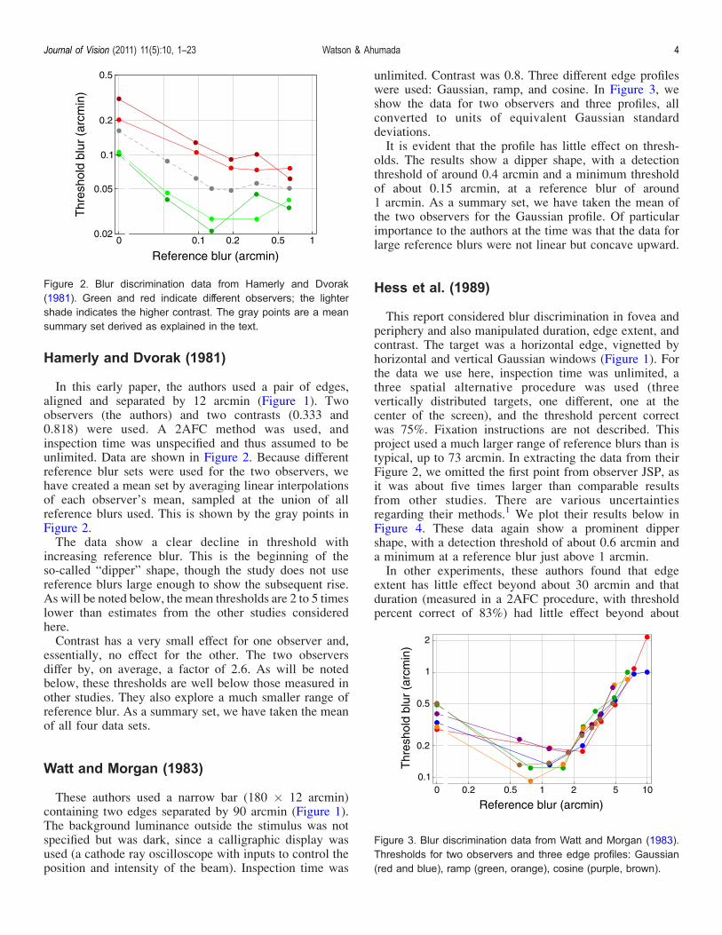
This report considered blur discrimination in fovea andperiphery and also manipulated duration, edge extent, andcontrast. The target was a horizontal edge, vignetted byhorizontal and vertical Gaussian windows (Figure 1). Forthe data we use here, inspection time was unlimited, athree spatial alternative procedure was used (threevertically distributed targets, one different, one at thecenter of the screen), and the threshold percent correctwas 75%. Fixation instructions are not described. Thisproject used a much larger range of reference blurs than istypical, up to 73 arcmin. In extracting the data from theirFigure 2, we omitted the first point from observer JSP, asit was about five times larger than comparable resultsfrom other studies. There are various uncertaintiesregarding their methods.1 We plot their results below inFigure 4. These data again show a prominent dippershape, with a detection threshold of about 0.6 arcmin anda minimum at a reference blur just above 1 arcmin.In other experiments, these authors found that edge

extent has little effect beyond about 30 arcmin and thatduration (measured in a 2AFC procedure, with thresholdpercent correct of 83%) had little effect beyond about

Figure 2. Blur discrimination data from Hamerly and Dvorak(1981). Green and red indicate different observers; the lightershade indicates the higher contrast. The gray points are a meansummary set derived as explained in the text.

Figure 3. Blur discrimination data from Watt and Morgan (1983).Thresholds for two observers and three edge profiles: Gaussian(red and blue), ramp (green, orange), cosine (purple, brown).


60 ms (both measures expressed as 1/e Gaussian half-widths). They also found that contrasts above 0.3produced little or no change in thresholds, but thatcontrasts of 0.05 and 0.02 did produce appreciably higherthresholds.

Pääkkönen and Morgan (1994)

This report was concerned mainly with the effect ofmotion on blur discrimination but included a zero motioncondition. The target was a narrow bar (20 � 140 arcmin)bisected by a Gaussian edge (Figure 1). A 2IFC methodwas used, and the threshold percent correct was 83%. Thecontrast was 0.35, and the duration was 150 ms. Data werecollected from three observers and are shown in Figure 5.The dipper is again evident, with results similar to thoseof Watt and Morgan (1983).

Wuerger et al. (2001)

This study considered blur discrimination in bothluminance and chromatic domains. Here, we consideronly the luminance data (Wuerger et al., 2001). Theirtarget was a 1 cycle/deg square wave, blurred by aGaussian, and vignetted by a Gaussian with standarddeviation of 2 deg (Figure 1). Duration was 1 s, andcontrast was 0.1. A 2IFC method was used, and fourobservers participated. It was not possible to extractindividual observers from their Figure 1, so we have onlyextracted the mean, as shown here in Figure 6. These dataagain show a dipper. They are similar but somewhathigher than the previous two studies.

Mather and Smith (2002)

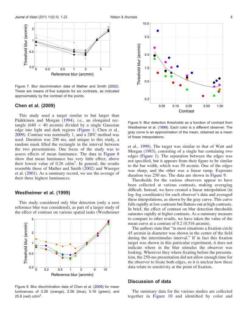
This study is primarily about blur as a cue to depth butincludes blur discrimination thresholds for a range ofreference blurs and contrasts (Mather & Smith, 2002). Thetarget was a 4.36-deg square separated into bright anddark halves by a sinusoidally curving border (2 cycles/image, amplitude = 0.15 image; Figure 1). A 2IFC methodwas used, with two 0.5-s exposures separated by a 1-s gap.No feedback was given. The interval and remainder of thescreen were filled with a luminance equal to the mean ofbright and dark regions. Five subjects took part, but onlymean data were shown. Five different contrasts were usedin separate sessions: 0.1, 0.2, 0.4, 0.6, 0.68, and 0.8. Theseresults are shown in Figure 7.It is evident that contrast has little or no effect, except at

the lowest value of 0.1. The pattern of results is similar tothe previous studies, and the thresholds resemble those ofWuerger et al. (2001). As a summary set, we have takenthe mean of the data from the highest four contrasts, overwhich thresholds differed little.

Figure 5. Blur discrimination data from Pääkkönen and Morgan(1994). Thresholds for three observers.

Figure 6. Blur discrimination data of Wuerger et al. (2001). Theseare means of four observers.

Figure 4. Blur discrimination data from Hess et al. (1989) for twoobservers.


Chen et al. (2009)

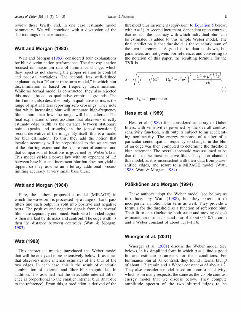
This study used a target similar to but larger thanPaakkonen and Morgan (1994), i.e., an elongated rec-tangle (640 � 40 arcmin) divided by a single Gaussianedge into light and dark regions (Figure 1; Chen et al.,2009). Contrast was nominally 1, and a 2IFC method wasused. Duration was 200 ms, and unique to this study, arandom mask filled the rectangle in the interval betweenthe two presentations. One focus of the study was toassess effects of mean luminance. The data in Figure 8show that mean luminance has very little effect, abovetheir lowest value of 0.26 cd/m2. In general, the resultsresemble those of Mather and Smith (2002) and Wuergeret al. (2001). As a summary record, we use the average oftheir three highest luminances.

Westheimer et al. (1999)

This study considered only blur detection (only a zeroreference blur was considered), as part of a larger study ofthe effect of contrast on various spatial tasks (Westheimer

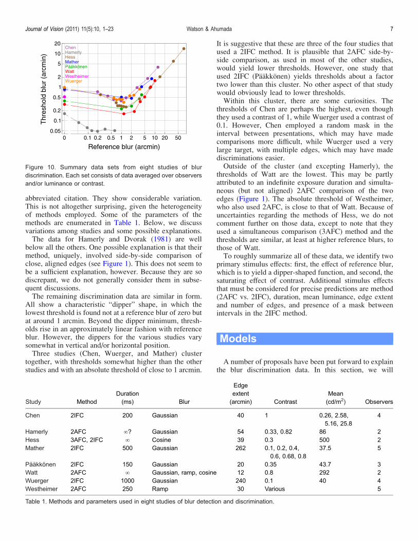
et al., 1999). The target was similar to that of Watt andMorgan (1983), consisting of a single bar containing twoedges (Figure 1). The separation between the edges wasnot specified, but it appears from their figure to be similarto the bar width, which was 30 arcmin. One of the edgeswas sharp, and the other was a linear ramp. Exposureduration was 250 ms. The data are shown in Figure 9.Thresholds for the various observers appear to have

been collected at various contrasts, making averagingdifficult. Instead, we have created a linear interpolation (inlog–log coordinates) for each observer’s data and averagedthese interpolations, as shown by the gray curve. This curvefalls rapidly at low contrasts but flattens out at high contrasts.In brief, the effect of contrast on blur detection thresholdssaturates rapidly at higher contrasts. As a summary measureto compare to other results, we have taken the value of themean curve at a contrast of 0.2 (0.516 arcmin).The authors state that “in most situations a fixation circle

45 arcmin in diameter was shown in the center of the fieldduring the interstimulus interval.” If in fact this fixationtarget was shown in this particular experiment, it does notindicate where in the blur stimulus the observer waslooking. Wherever they where fixating before the presenta-tion, the 250-ms presentation did not allow enough time forthe observer to fixate both edges, so it is unclear how thesedata relate to sensitivity at the point of fixation.

Discussion of data

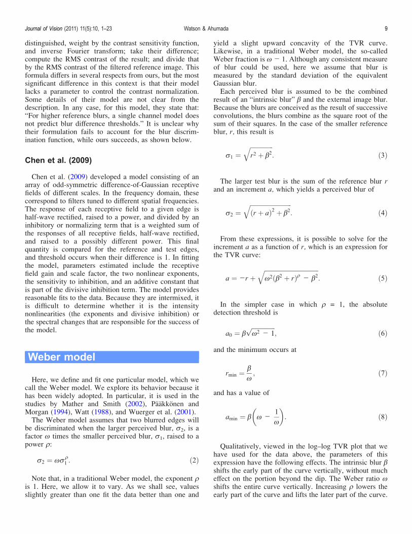
The summary data for the various studies are collectedtogether in Figure 10 and identified by color and

Figure 8. Blur discrimination data of Chen et al. (2009) for meanluminances of 0.26 (orange), 2.58 (blue), 5.16 (green), and25.8 (red) cd/m2.

Figure 9. Blur detection thresholds as a function of contrast fromWestheimer et al. (1999). Each color is a different observer. Thegray curve is an approximation of the mean, obtained as a meanof linear interpolations.

Figure 7. Blur discrimination data of Mather and Smith (2002).These are means of five subjects for six contrasts, as indicatedapproximately by the contrast of the points.


abbreviated citation. They show considerable variation.This is not altogether surprising, given the heterogeneityof methods employed. Some of the parameters of themethods are enumerated in Table 1. Below, we discussvariations among studies and some possible explanations.The data for Hamerly and Dvorak (1981) are well

below all the others. One possible explanation is that theirmethod, uniquely, involved side-by-side comparison ofclose, aligned edges (see Figure 1). This does not seem tobe a sufficient explanation, however. Because they are sodiscrepant, we do not generally consider them in subse-quent discussions.The remaining discrimination data are similar in form.

All show a characteristic “dipper” shape, in which thelowest threshold is found not at a reference blur of zero butat around 1 arcmin. Beyond the dipper minimum, thresh-olds rise in an approximately linear fashion with referenceblur. However, the dippers for the various studies varysomewhat in vertical and/or horizontal position.Three studies (Chen, Wuerger, and Mather) cluster

together, with thresholds somewhat higher than the otherstudies and with an absolute threshold of close to 1 arcmin.

It is suggestive that these are three of the four studies thatused a 2IFC method. It is plausible that 2AFC side-by-side comparison, as used in most of the other studies,would yield lower thresholds. However, one study thatused 2IFC (Paakkonen) yields thresholds about a factortwo lower than this cluster. No other aspect of that studywould obviously lead to lower thresholds.Within this cluster, there are some curiosities. The

thresholds of Chen are perhaps the highest, even thoughthey used a contrast of 1, while Wuerger used a contrast of0.1. However, Chen employed a random mask in theinterval between presentations, which may have madecomparisons more difficult, while Wuerger used a verylarge target, with multiple edges, which may have madediscriminations easier.Outside of the cluster (and excepting Hamerly), the

thresholds of Watt are the lowest. This may be partlyattributed to an indefinite exposure duration and simulta-neous (but not aligned) 2AFC comparison of the twoedges (Figure 1). The absolute threshold of Westheimer,who also used 2AFC, is close to that of Watt. Because ofuncertainties regarding the methods of Hess, we do notcomment further on those data, except to note that theyused a simultaneous comparison (3AFC) method and thethresholds are similar, at least at higher reference blurs, tothose of Watt.To roughly summarize all of these data, we identify two

primary stimulus effects: first, the effect of reference blur,which is to yield a dipper-shaped function, and second, thesaturating effect of contrast. Additional stimulus effectsthat must be considered for precise predictions are method(2AFC vs. 2IFC), duration, mean luminance, edge extentand number of edges, and presence of a mask betweenintervals in the 2IFC method.

Models

A number of proposals have been put forward to explainthe blur discrimination data. In this section, we will

Figure 10. Summary data sets from eight studies of blurdiscrimination. Each set consists of data averaged over observersand/or luminance or contrast.

Study MethodDuration(ms) Blur

Edgeextent(arcmin) Contrast

Mean(cd/m2) Observers

Chen 2IFC 200 Gaussian 40 1 0.26, 2.58,5.16, 25.8

4

Hamerly 2AFC V? Gaussian 54 0.33, 0.82 86 2Hess 3AFC, 2IFC V Cosine 39 0.3 500 2Mather 2IFC 500 Gaussian 262 0.1, 0.2, 0.4,

0.6, 0.68, 0.837.5 5

Pääkkönen 2IFC 150 Gaussian 20 0.35 43.7 3Watt 2AFC V Gaussian, ramp, cosine 12 0.8 292 2Wuerger 2IFC 1000 Gaussian 240 0.1 40 4Westheimer 2AFC 250 Ramp 30 Various 5

Table 1. Methods and parameters used in eight studies of blur detection and discrimination.


review these briefly and, in one case, estimate modelparameters. We will conclude with a discussion of theshortcomings of these models.


Watt and Morgan (1983) considered four explanationsfor blur discrimination performance. The first explanationfocused on maximum rate of luminance change, whichthey reject as not showing the proper relation to contrastand pedestal variations. The second, less well-definedexplanation, is a “Fourier transform model,” in which blurdiscrimination is based on frequency discrimination.While no formal model is constructed, they also rejectedthis model based on qualitative empirical grounds. Thethird model, also described only in qualitative terms, is therange of spatial filters reporting zero crossings. They notethat while increasing blur will attenuate high-frequencyfilters more than low, the range will be unaltered. Thefinal explanation offered assumes that observers directlyestimate edge width as the distance between stationarypoints (peaks and troughs) in the (one-dimensional)second derivative of the image. By itself, this is a modelfor blur estimation. To this, they add the notion thatlocation accuracy will be proportional to the square rootof the blurring extent and the square root of contrast andthat comparison of locations is governed by Weber’s law.This model yields a power law with an exponent of 1.5between base blur and increment blur but does not yield adipper, so they assume an arbitrary additional processlimiting accuracy at very small base blurs.


Here, the authors proposed a model (MIRAGE) inwhich the waveform is processed by a range of band-passfilters and each output is split into positive and negativeparts. The positive and negative signals from the severalfilters are separately combined. Each zero bounded regionis then marked by its mass and centroid. The edge width isthen the distance between centroids (Watt & Morgan,1983).

Watt (1988)

This theoretical treatise introduced the Weber modelthat will be analyzed more extensively below. It assumesthat observers make internal estimates of the blur of thetwo edges. In each case, this is the result of quadraticcombination of external and filter blur magnitudes. Inaddition, it is assumed that the detectable internal differ-ence is proportional to the smaller internal blur (that dueto the reference). From this, a prediction is derived of the

threshold blur increment (equivalent to Equation 5 below,with > = 1). A second increment, dependent upon contrast,that reflects the accuracy with which individual blurs canbe estimated is added to this simple Weber model. Thefinal prediction is that threshold is the quadratic sum ofthe two increments. A good fit to data is shown, butparameters are not given. For reference, and converting tothe notation of this paper, the resulting formula for theTVR is

a ¼ffiffiffiffiffiffiffiffiffiffiffiffiffiffiffiffiffiffiffiffiffiffiffiffiffiffiffiffiffiffiffiffiffiffiffiffiffiffiffiffiffiffiffiffiffiffiffiffiffiffiffiffiffiffiffiffiffiffiffiffiffiffiffiffiffiffiffiffiffiffiffiffiffiffiffiffiffiffiffiffiffiffiffiffiffiffiffiffiffiffiffiffiffiffir j

ffiffiffiffiffiffiffiffiffiffiffiffiffiffiffiffiffiffiffiffiffiffiffiffiffiffiffiffiffiffiffiffiffiffiffiffiffiffið52 j 1Þ"2 þ r252

q� �2

þ ðr2 þ "2Þ3=2kL2c"3

s;

ð1Þ

where kL is a parameter.

Hess et al. (1989)

Hess et al. (1989) first considered an array of Gaborfilters, with sensitivities governed by the overall contrastsensitivity function, with outputs subject to an accelerat-ing nonlinearity. The energy response of a filter of aparticular center spatial frequency to changes in the blurof an edge was then computed to determine the thresholdblur increment. The overall threshold was assumed to bethat due to the most sensitive filter. They later abandonthis model, as it is inconsistent with their data from phase-shifted edges, and resort to a MIRAGE model (Watt,1988; Watt & Morgan, 1984).

Pääkkönen and Morgan (1994)

These authors adopt the Weber model (see below) asintroduced by Watt (1988), but they extend it toincorporate a motion blur term as well. They provide aformula for the threshold as a function of reference blur.Their fit to data (including both static and moving edges)estimated an intrinsic spatial blur of about 0.5–0.7 arcminand a Weber constant of about 1.11–1.16.

Wuerger et al. (2001)

Wuerger et al. (2001) discuss the Weber model (seebelow), in its simplified form in which > = 1, find a goodfit, and estimate parameters for their conditions. Forluminance blur at 0.1 contrast, they found internal blur "of about 1.2 arcmin and a Weber constant 5 of about 1.2.They also consider a model based on contrast sensitivity,which is, in many respects, the same as the visible contrastenergy model that we discuss below. They computeamplitude spectra of the two blurred edges to be


distinguished, weight by the contrast sensitivity function,and inverse Fourier transform; take their difference;compute the RMS contrast of the result; and divide thatby the RMS contrast of the filtered reference image. Thisformula differs in several respects from ours, but the mostsignificant difference in this context is that their modellacks a parameter to control the contrast normalization.Some details of their model are not clear from thedescription. In any case, for this model, they state that:“For higher reference blurs, a single channel model doesnot predict blur difference thresholds.” It is unclear whytheir formulation fails to account for the blur discrim-ination function, while ours succeeds, as shown below.

Chen et al. (2009)

Chen et al. (2009) developed a model consisting of anarray of odd-symmetric difference-of-Gaussian receptivefields of different scales. In the frequency domain, thesecorrespond to filters tuned to different spatial frequencies.The response of each receptive field to a given edge ishalf-wave rectified, raised to a power, and divided by aninhibitory or normalizing term that is a weighted sum ofthe responses of all receptive fields, half-wave rectified,and raised to a possibly different power. This finalquantity is compared for the reference and test edges,and threshold occurs when their difference is 1. In fittingthe model, parameters estimated include the receptivefield gain and scale factor, the two nonlinear exponents,the sensitivity to inhibition, and an additive constant thatis part of the divisive inhibition term. The model providesreasonable fits to the data. Because they are intermixed, itis difficult to determine whether it is the intensitynonlinearities (the exponents and divisive inhibition) orthe spectral changes that are responsible for the success ofthe model.

Weber model

Here, we define and fit one particular model, which wecall the Weber model. We explore its behavior because ithas been widely adopted. In particular, it is used in thestudies by Mather and Smith (2002), Paakkonen andMorgan (1994), Watt (1988), and Wuerger et al. (2001).The Weber model assumes that two blurred edges will

be discriminated when the larger perceived blur, A2, is afactor 5 times the smaller perceived blur, A1, raised to apower >:

A2 ¼ 5A>1 : ð2Þ

Note that, in a traditional Weber model, the exponent >is 1. Here, we allow it to vary. As we shall see, valuesslightly greater than one fit the data better than one and

yield a slight upward concavity of the TVR curve.Likewise, in a traditional Weber model, the so-calledWeber fraction is 5 j 1. Although any consistent measureof blur could be used, here we assume that blur ismeasured by the standard deviation of the equivalentGaussian blur.Each perceived blur is assumed to be the combined

result of an “intrinsic blur” " and the external image blur.Because the blurs are conceived as the result of successiveconvolutions, the blurs combine as the square root of thesum of their squares. In the case of the smaller referenceblur, r, this result is

A1 ¼ffiffiffiffiffiffiffiffiffiffiffiffiffiffiffir2 þ "2

q: ð3Þ

The larger test blur is the sum of the reference blur rand an increment a, which yields a perceived blur of

A2 ¼ffiffiffiffiffiffiffiffiffiffiffiffiffiffiffiffiffiffiffiffiffiffiffiffiffiffiffiðr þ aÞ2 þ "2

q: ð4Þ

From these expressions, it is possible to solve for theincrement a as a function of r, which is an expression forthe TVR curve:

a ¼ jr þffiffiffiffiffiffiffiffiffiffiffiffiffiffiffiffiffiffiffiffiffiffiffiffiffiffiffiffiffiffiffiffiffiffiffi52ð"2 þ rÞ> j "2

q: ð5Þ

In the simpler case in which > = 1, the absolutedetection threshold is

a0 ¼ "ffiffiffiffiffiffiffiffiffiffiffiffiffiffiffi52 j 1

p; ð6Þ

and the minimum occurs at

rmin ¼ "

5; ð7Þ

and has a value of

amin ¼ " 5 j1

5

� �: ð8Þ

Qualitatively, viewed in the log–log TVR plot that wehave used for the data above, the parameters of thisexpression have the following effects. The intrinsic blur "shifts the early part of the curve vertically, without mucheffect on the portion beyond the dip. The Weber ratio 5shifts the entire curve vertically. Increasing > lowers theearly part of the curve and lifts the later part of the curve.


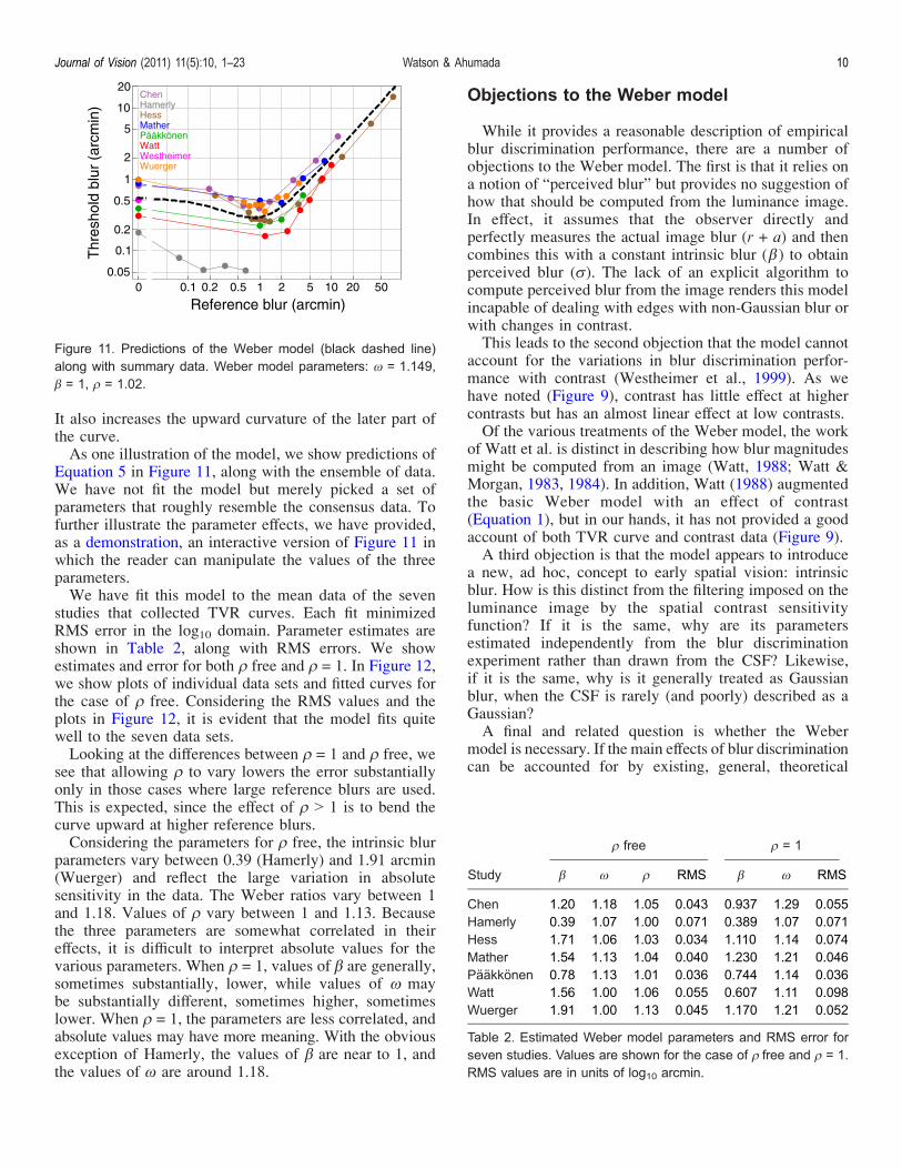
It also increases the upward curvature of the later part ofthe curve.As one illustration of the model, we show predictions of

Equation 5 in Figure 11, along with the ensemble of data.We have not fit the model but merely picked a set ofparameters that roughly resemble the consensus data. Tofurther illustrate the parameter effects, we have provided,as a demonstration, an interactive version of Figure 11 inwhich the reader can manipulate the values of the threeparameters.We have fit this model to the mean data of the seven

studies that collected TVR curves. Each fit minimizedRMS error in the log10 domain. Parameter estimates areshown in Table 2, along with RMS errors. We showestimates and error for both > free and > = 1. In Figure 12,we show plots of individual data sets and fitted curves forthe case of > free. Considering the RMS values and theplots in Figure 12, it is evident that the model fits quitewell to the seven data sets.Looking at the differences between > = 1 and > free, we

see that allowing > to vary lowers the error substantiallyonly in those cases where large reference blurs are used.This is expected, since the effect of > 9 1 is to bend thecurve upward at higher reference blurs.Considering the parameters for > free, the intrinsic blur

parameters vary between 0.39 (Hamerly) and 1.91 arcmin(Wuerger) and reflect the large variation in absolutesensitivity in the data. The Weber ratios vary between 1and 1.18. Values of > vary between 1 and 1.13. Becausethe three parameters are somewhat correlated in theireffects, it is difficult to interpret absolute values for thevarious parameters. When > = 1, values of " are generally,sometimes substantially, lower, while values of 5 maybe substantially different, sometimes higher, sometimeslower. When > = 1, the parameters are less correlated, andabsolute values may have more meaning. With the obviousexception of Hamerly, the values of " are near to 1, andthe values of 5 are around 1.18.

Objections to the Weber model

While it provides a reasonable description of empiricalblur discrimination performance, there are a number ofobjections to the Weber model. The first is that it relies ona notion of “perceived blur” but provides no suggestion ofhow that should be computed from the luminance image.In effect, it assumes that the observer directly andperfectly measures the actual image blur (r + a) and thencombines this with a constant intrinsic blur (") to obtainperceived blur (A). The lack of an explicit algorithm tocompute perceived blur from the image renders this modelincapable of dealing with edges with non-Gaussian blur orwith changes in contrast.This leads to the second objection that the model cannot

account for the variations in blur discrimination perfor-mance with contrast (Westheimer et al., 1999). As wehave noted (Figure 9), contrast has little effect at highercontrasts but has an almost linear effect at low contrasts.Of the various treatments of the Weber model, the work

of Watt et al. is distinct in describing how blur magnitudesmight be computed from an image (Watt, 1988; Watt &Morgan, 1983, 1984). In addition, Watt (1988) augmentedthe basic Weber model with an effect of contrast(Equation 1), but in our hands, it has not provided a goodaccount of both TVR curve and contrast data (Figure 9).A third objection is that the model appears to introduce

a new, ad hoc, concept to early spatial vision: intrinsicblur. How is this distinct from the filtering imposed on theluminance image by the spatial contrast sensitivityfunction? If it is the same, why are its parametersestimated independently from the blur discriminationexperiment rather than drawn from the CSF? Likewise,if it is the same, why is it generally treated as Gaussianblur, when the CSF is rarely (and poorly) described as aGaussian?A final and related question is whether the Weber

model is necessary. If the main effects of blur discriminationcan be accounted for by existing, general, theoretical

Figure 11. Predictions of the Weber model (black dashed line)along with summary data. Weber model parameters: 5 = 1.149," = 1, > = 1.02.

Study

> free > = 1

" 5 > RMS " 5 RMS

Chen 1.20 1.18 1.05 0.043 0.937 1.29 0.055Hamerly 0.39 1.07 1.00 0.071 0.389 1.07 0.071Hess 1.71 1.06 1.03 0.034 1.110 1.14 0.074Mather 1.54 1.13 1.04 0.040 1.230 1.21 0.046Pääkkönen 0.78 1.13 1.01 0.036 0.744 1.14 0.036Watt 1.56 1.00 1.06 0.055 0.607 1.11 0.098Wuerger 1.91 1.00 1.13 0.045 1.170 1.21 0.052

Table 2. Estimated Weber model parameters and RMS error forseven studies. Values are shown for the case of > free and > = 1.RMS values are in units of log10 arcmin.



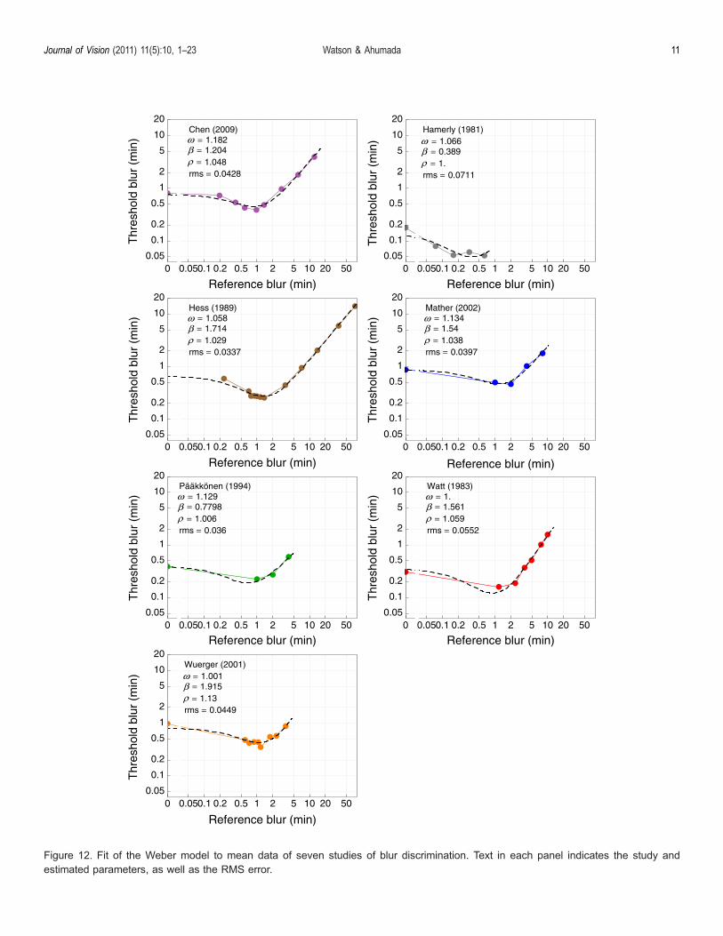
Figure 12. Fit of the Weber model to mean data of seven studies of blur discrimination. Text in each panel indicates the study andestimated parameters, as well as the RMS error.


formulations, then there is no need to construct a specialad hoc model for the case of blur discrimination. As wewill argue in the next section, such a model does exist inthe form of visible contrast energy discrimination.

Visible contrast energydiscrimination

In the previous section, we questioned whether a modeldesigned uniquely to deal with blur discrimination wasnecessary or whether the results could be accounted for byexisting general models of contrast discrimination. In thissection, we describe two such models. The first isparticularly simple and is presented to show that theessentials of the TVR curve are a consequence of thenature of difference signal and the contrast sensitivityfunction alone. In the second model, we add a smallamount of complexity, in the form of local contrast andmasking by local contrast energy, in order to betteraccount for the saturating effect of contrast on blurdiscrimination. We call these two models visible contrastenergy (ViCE) and ViCE simplified (ViCEs).

Simplified model (ViCEs)

In this model, we assume that two blurred edges arediscriminated when the contrast energy of their difference,after filtering by the contrast sensitivity function (CSF), isequal to a criterion value. In this derivation, we make useof a canonical function, which we call a unit Gaussian. Inthe space domain, a unit Gaussian with positive scale s isgiven by

G x; sð Þ ¼ 1

sexp j:

x2

s2

� �: ð9Þ

This has a maximum of 1/s and an integral of 1. The scales is an alternative to the standard deviation as a measureof the Gaussian width. The two are related by

A ¼ sffiffiffiffiffiffi2:

p : ð10Þ

A unit Gaussian in the frequency domain is given by

G~ðu; sÞ ¼ expðj:s2u2Þ: ð11Þ

This has a maximum of 1 and an integral of 1/s. It is theFourier transform of G(x, s). An attractive feature of this

parameterization of Gaussians is that the Fourier trans-form of a Gaussian of scale s (in degrees) is a Gaussian ofscale 1/s (in cycles/degree).An ideal unit contrast edge can be represented by the

sign (sgn) function. The reference and test blurred edgescan be represented by convolution with Gaussians ofscales rVand rV+ aV, respectively:

Gðx; rVÞ � sgnðxÞ; Gðx; rVþ aVÞ � sgnðxÞ: ð12Þ

We use primes to indicate that the quantities representscales, converted from the corresponding standard devia-tions by Equation 10. Note that the two edge blurringGaussians differ in width, but both have the same unitarea.We represent the CSF, in the space domain, as a

difference of Gaussians (DoG), with center scale 7 andsurround scale E, with a surround weight of 1 and gain + .The parameter 1 lies between 0 and 1 and represents theratio of areas of the two Gaussians:

+½Gðx;7Þj 1Gðx; EÞ�: ð13Þ

To compute the contrast energy difference between thetwo blurred edges, we convolve each with the CSF,subtract the results, and then square and integrate thedifference. Because convolution is linear, we can rear-range terms and subtract the edge blurring kernels first,followed by convolution with the ideal edge and the CSF.Including the edge contrast c, the visible contrast energydifference can thus be written as

V ¼ c2+2Z V

jV

��½Gðx; rVÞ j Gðx; rVþ aVÞ� � sgnðxÞ� ½Gðx;7Þ j 1Gðx; EÞ��2: ð14Þ

According to Plancherel’s theorem, a function and itsFourier transform have equal energy. Thus, Equation 14can be rewritten by Fourier transforming the elementswithin the absolute value. The unit Gaussians transform tounit Gaussians, the sgn function transforms to animaginary hyperbola, and convolutions transform tomultiplications, giving us

V ¼ c2+2Z V

jV

��½G~ðu; rVÞ j G~ u; rVþ aVð Þ� �ji

:u

� G~ u;7ð Þ j 1G~ u; Eð Þ� ��2: ð15Þ

Note that the difference of Gaussians on the right nowrepresents a CSF in the frequency domain. The parameter 1,


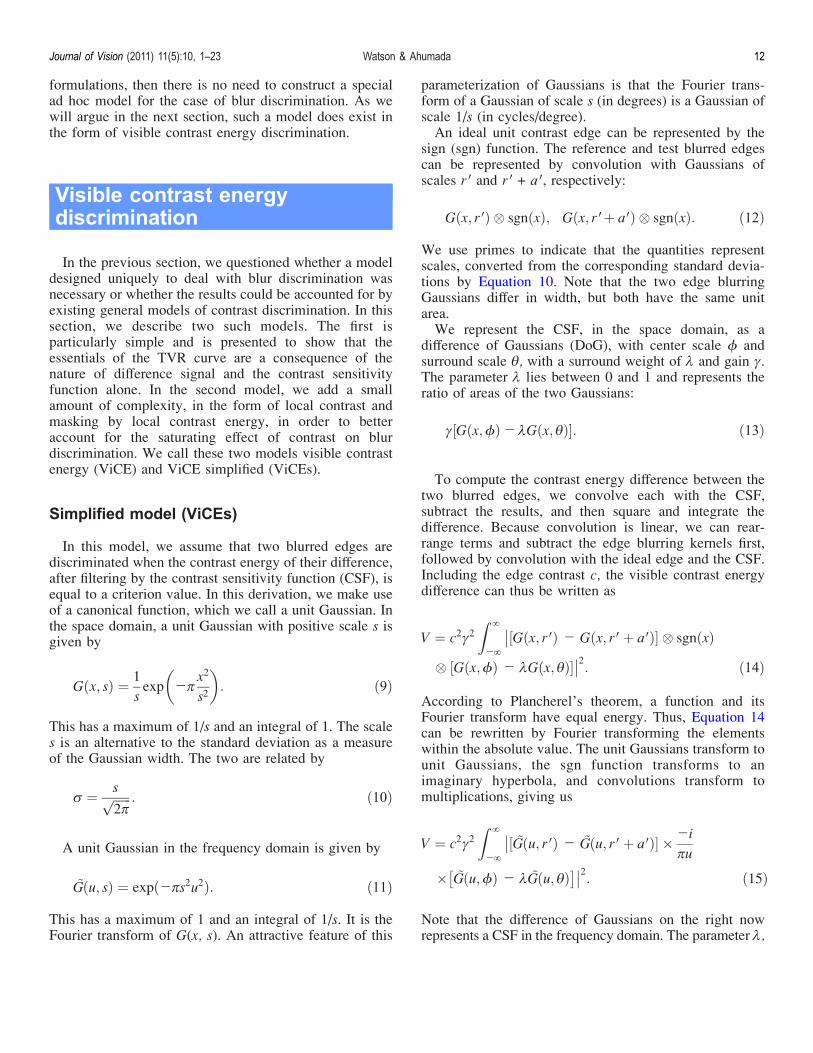
introduced above, determines the attenuation at low spatialfrequencies.The steps in this derivation are also illustrated in Figure 13,

which shows them in the form of a graphic equation. Thefirst row shows the elements of the model in the spacedomain, and the second row shows them in the Fourierdomain. The last row shows that the final result is theenergy of the product of two functions: one is thedifference of the two blur spectra (the leftmost two termsin row two), and the other is the product of the CSF andthe hyperbola (the rightmost three terms in row two). It isconvenient to segregate the terms in this way because theformer is what is manipulated in the experiment and thelatter is fixed.A convenient and remarkable feature of this model is

that the integral has a solution, which simplifies thecalculation of predictions. For reference, we provide ithere. In this expression, aV, rV, 7, and E are Gaussianscales expressed in degrees, and V is the visible contrastenergy:

V ¼ j1

:2c2+2

ffiffiffi2

p12

ffiffiffiffiffiffiffiffiffiffiffiffiffiffiffiffiffiffiffiffiE2 þ ðrVÞ2

qþ

ffiffiffi2

p ffiffiffiffiffiffiffiffiffiffiffiffiffiffiffiffiffiffiffiffiffi72 þ ðrVÞ2

q

j 21

ffiffiffiffiffiffiffiffiffiffiffiffiffiffiffiffiffiffiffiffiffiffiffiffiffiffiffiffiffiffiffiffiffiE2 þ 72 þ 2ðr 0 Þ2

qj 212

ffiffiffiffiffiffiffiffiffiffiffiffiffiffiffiffiffiffiffiffiffiffiffiffiffiffiffiffiffiffiffiffiffiffiffiffiffiffiffiffiffiffiffiffiffiffiffiffiffiffiffiffiffiffiffiffiffi2E2 þ ða 0 Þ2 þ 2a 0r 0 þ 2ðr 0 Þ2

q

þ 41

ffiffiffiffiffiffiffiffiffiffiffiffiffiffiffiffiffiffiffiffiffiffiffiffiffiffiffiffiffiffiffiffiffiffiffiffiffiffiffiffiffiffiffiffiffiffiffiffiffiffiffiffiffiffiffiffiffiffiffiffiffiffiffiffiffiE2 þ 72 þ ða 0 Þ2 þ 2a 0r 0 þ 2ðr 0 Þ2

q

j 2

ffiffiffiffiffiffiffiffiffiffiffiffiffiffiffiffiffiffiffiffiffiffiffiffiffiffiffiffiffiffiffiffiffiffiffiffiffiffiffiffiffiffiffiffiffiffiffiffiffiffiffiffiffiffiffiffiffiffi272 þ ða 0 Þ2 þ 2a 0r 0 þ 2ðr 0 Þ2

qþ

ffiffiffi2

p12

ffiffiffiffiffiffiffiffiffiffiffiffiffiffiffiffiffiffiffiffiffiffiffiffiffiffiffiffiffiffiE2 þ ða 0 þ r 0 Þ2

q

þffiffiffi2

p ffiffiffiffiffiffiffiffiffiffiffiffiffiffiffiffiffiffiffiffiffiffiffiffiffiffiffiffiffiffiffi72 þ ða 0 þ r 0 Þ2

qj 21

ffiffiffiffiffiffiffiffiffiffiffiffiffiffiffiffiffiffiffiffiffiffiffiffiffiffiffiffiffiffiffiffiffiffiffiffiffiffiffiffiffiffiffiffiE2 þ 72 þ 2ða 0 þ r 0 Þ2

q !: ð16Þ

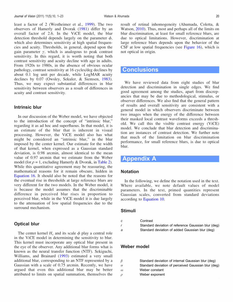
In the visible contrast energy model, a signal is detectedwhen the energy V = 1. In order to generate predictions forthis model, we require values for the parameters 7, E, + ,and 1. We have obtained these values through anapproximate fit to a set of eleven contrast thresholds forGabor functions from the ModelFest experiment (Carneyet al., 2000; Watson & Ahumada, 2005). All of thesetargets employed a Gaussian aperture with a standarddeviation of 0.5 deg. The first target, with a nominalspatial frequency of 0, was actually a simple Gaussian,with no sinusoidal modulation. That target is useful forestimating the sensitivity to very low spatial frequencies.In this fitting procedure, we are aided by the fact that

the response of this model to a Gabor target has also aclosed form solution (Appendix A). Because the DoGCSF falls much more rapidly than the human data, we haveelected to omit the highest frequency Gabor (30 cycles/deg)from the fit. The result of this fit is shown in Figure 14.The estimates obtained were + = 160.05, 1 = 0.7329, 7 =2.456 arcmin, and E = 24.75 arcmin.2

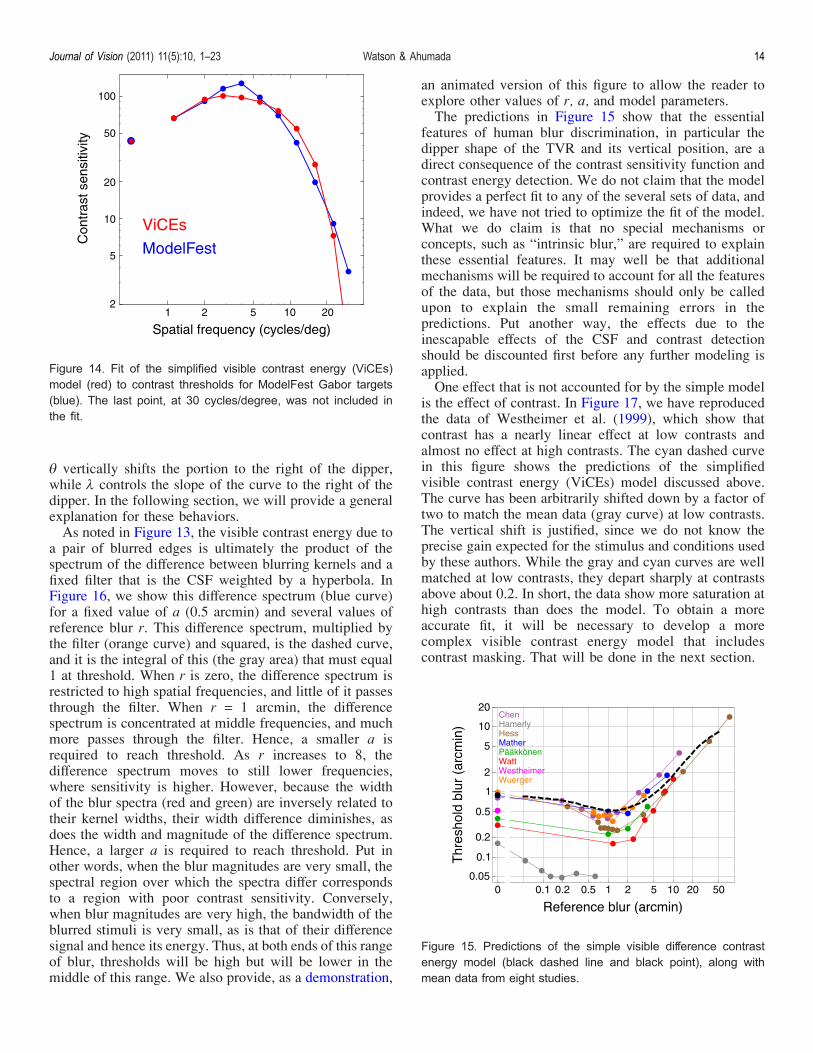
Using the estimated parameters, for each value ofreference blur r, we can solve for the value of added blurthat yields V = 1. A result is shown in Figure 15 for anedge contrast of c = 0.2. This figure shows that thesimplest visible contrast energy model, with no adjust-ment of parameters, predicts the essential features of theblur discrimination TVR function: the absolute threshold,the dipper, the location of the dip, the magnitude of thedip, and the rise at higher reference blurs.To allow the reader to explore the effects of the various

model parameters, we provide, as a demonstration, aninteractive version of Figure 15 that allows modificationof the parameters. This shows that, in the log–log plot,+ generally shifts the predictions vertically, 7 verticallyshifts the portion of the curve to the left of the dipper,

Figure 13. Graphic representation of the derivation of the simple version of the visible contrast energy model. The first row shows (left)blurring Gaussians, (center) step edge, and (right) difference-of-Gaussian receptive field. The second row shows these elements afterFourier transformation. In the third row, we show that the final result is the energy of the product of two functions: one is the difference ofthe two blur spectra, and the other is the product of the CSF and the hyperbola.



E vertically shifts the portion to the right of the dipper,while 1 controls the slope of the curve to the right of thedipper. In the following section, we will provide a generalexplanation for these behaviors.As noted in Figure 13, the visible contrast energy due to

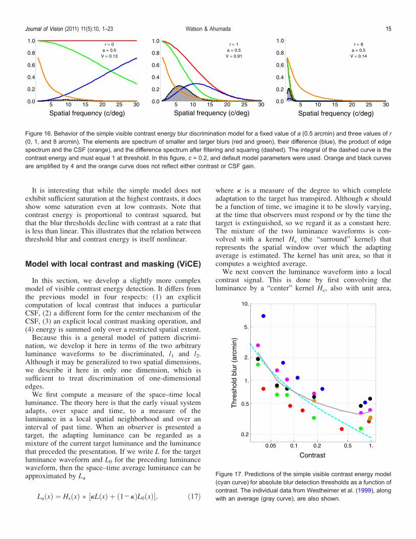
a pair of blurred edges is ultimately the product of thespectrum of the difference between blurring kernels and afixed filter that is the CSF weighted by a hyperbola. InFigure 16, we show this difference spectrum (blue curve)for a fixed value of a (0.5 arcmin) and several values ofreference blur r. This difference spectrum, multiplied bythe filter (orange curve) and squared, is the dashed curve,and it is the integral of this (the gray area) that must equal1 at threshold. When r is zero, the difference spectrum isrestricted to high spatial frequencies, and little of it passesthrough the filter. When r = 1 arcmin, the differencespectrum is concentrated at middle frequencies, and muchmore passes through the filter. Hence, a smaller a isrequired to reach threshold. As r increases to 8, thedifference spectrum moves to still lower frequencies,where sensitivity is higher. However, because the widthof the blur spectra (red and green) are inversely related totheir kernel widths, their width difference diminishes, asdoes the width and magnitude of the difference spectrum.Hence, a larger a is required to reach threshold. Put inother words, when the blur magnitudes are very small, thespectral region over which the spectra differ correspondsto a region with poor contrast sensitivity. Conversely,when blur magnitudes are very high, the bandwidth of theblurred stimuli is very small, as is that of their differencesignal and hence its energy. Thus, at both ends of this rangeof blur, thresholds will be high but will be lower in themiddle of this range. We also provide, as a demonstration,

an animated version of this figure to allow the reader toexplore other values of r, a, and model parameters.The predictions in Figure 15 show that the essential

features of human blur discrimination, in particular thedipper shape of the TVR and its vertical position, are adirect consequence of the contrast sensitivity function andcontrast energy detection. We do not claim that the modelprovides a perfect fit to any of the several sets of data, andindeed, we have not tried to optimize the fit of the model.What we do claim is that no special mechanisms orconcepts, such as “intrinsic blur,” are required to explainthese essential features. It may well be that additionalmechanisms will be required to account for all the featuresof the data, but those mechanisms should only be calledupon to explain the small remaining errors in thepredictions. Put another way, the effects due to theinescapable effects of the CSF and contrast detectionshould be discounted first before any further modeling isapplied.One effect that is not accounted for by the simple model

is the effect of contrast. In Figure 17, we have reproducedthe data of Westheimer et al. (1999), which show thatcontrast has a nearly linear effect at low contrasts andalmost no effect at high contrasts. The cyan dashed curvein this figure shows the predictions of the simplifiedvisible contrast energy (ViCEs) model discussed above.The curve has been arbitrarily shifted down by a factor oftwo to match the mean data (gray curve) at low contrasts.The vertical shift is justified, since we do not know theprecise gain expected for the stimulus and conditions usedby these authors. While the gray and cyan curves are wellmatched at low contrasts, they depart sharply at contrastsabove about 0.2. In short, the data show more saturation athigh contrasts than does the model. To obtain a moreaccurate fit, it will be necessary to develop a morecomplex visible contrast energy model that includescontrast masking. That will be done in the next section.

Figure 15. Predictions of the simple visible difference contrastenergy model (black dashed line and black point), along withmean data from eight studies.

Figure 14. Fit of the simplified visible contrast energy (ViCEs)model (red) to contrast thresholds for ModelFest Gabor targets(blue). The last point, at 30 cycles/degree, was not included inthe fit.



It is interesting that while the simple model does notexhibit sufficient saturation at the highest contrasts, it doesshow some saturation even at low contrasts. Note thatcontrast energy is proportional to contrast squared, butthat the blur thresholds decline with contrast at a rate thatis less than linear. This illustrates that the relation betweenthreshold blur and contrast energy is itself nonlinear.

Model with local contrast and masking (ViCE)

In this section, we develop a slightly more complexmodel of visible contrast energy detection. It differs fromthe previous model in four respects: (1) an explicitcomputation of local contrast that induces a particularCSF, (2) a different form for the center mechanism of theCSF, (3) an explicit local contrast masking operation, and(4) energy is summed only over a restricted spatial extent.Because this is a general model of pattern discrimi-

nation, we develop it here in terms of the two arbitraryluminance waveforms to be discriminated, l1 and l2.Although it may be generalized to two spatial dimensions,we describe it here in only one dimension, which issufficient to treat discrimination of one-dimensionaledges.We first compute a measure of the space–time local

luminance. The theory here is that the early visual systemadapts, over space and time, to a measure of theluminance in a local spatial neighborhood and over aninterval of past time. When an observer is presented atarget, the adapting luminance can be regarded as amixture of the current target luminance and the luminancethat preceded the presentation. If we write L for the targetluminance waveform and L0 for the preceding luminancewaveform, then the space–time average luminance can beapproximated by La

LaðxÞ ¼ HsðxÞ * ½.LðxÞ þ ð1j.ÞL0ðxÞ�; ð17Þ

where . is a measure of the degree to which completeadaptation to the target has transpired. Although . shouldbe a function of time, we imagine it to be slowly varying,at the time that observers must respond or by the time thetarget is extinguished, so we regard it as a constant here.The mixture of the two luminance waveforms is con-volved with a kernel Hs (the “surround” kernel) thatrepresents the spatial window over which the adaptingaverage is estimated. The kernel has unit area, so that itcomputes a weighted average.We next convert the luminance waveform into a local

contrast signal. This is done by first convolving theluminance by a “center” kernel Hc, also with unit area,

Figure 17. Predictions of the simple visible contrast energy model(cyan curve) for absolute blur detection thresholds as a function ofcontrast. The individual data from Westheimer et al. (1999), alongwith an average (gray curve), are also shown.

Figure 16. Behavior of the simple visible contrast energy blur discrimination model for a fixed value of a (0.5 arcmin) and three values of r(0, 1, and 8 arcmin). The elements are spectrum of smaller and larger blurs (red and green), their difference (blue), the product of edgespectrum and the CSF (orange), and the difference spectrum after filtering and squaring (dashed). The integral of the dashed curve is thecontrast energy and must equal 1 at threshold. In this figure, c = 0.2, and default model parameters were used. Orange and black curvesare amplified by 4 and the orange curve does not reflect either contrast or CSF gain.


that reflects optical and perhaps neural blurring. From this,the local average is subtracted, which also divides theresult:

C xð Þ ¼ HcðxÞ * LðxÞ j LaðxÞLaðxÞ ¼ Hc * LðxÞ

LaðxÞ j 1:

ð18Þ

In many cases, the prior luminance waveform is a constantL0, in which case

C xð Þ ¼ HcðxÞ * LðxÞ.HsðxÞ * LðxÞ þ ð1 j .ÞL0 j 1: ð19Þ

For the center kernel, we use a hyperbolic secant with ascale 7 (in degrees):

Hc xð Þ ¼ 1

7sech :

x

7

� �: ð20Þ

Later, we will show that this provides a better fit to thehigh-frequency decline of the human CSF than does aGaussian.For the surround kernel, we use a unit Gaussian with

scale E (in degrees):

Hs xð Þ ¼ G x; Eð Þ ¼ 1

Eexp j:

x

E

� �2� �: ð21Þ

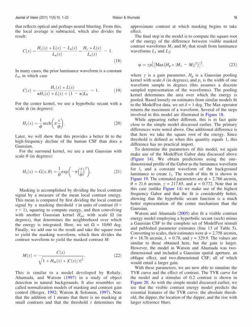
Masking is accomplished by dividing the local contrastsignal by a measure of the mean local contrast energy.This mean is computed by first dividing the local contrastsignal by a masking threshold C in units of contrast (0 GC G 1), squaring to compute energy, and then convolvingwith another Gaussian kernel Hm, with scale 4 (indegrees), that determines the neighborhood over whichthe energy is integrated. Here, we set 4 = 10/60 deg.Finally, we add one to the result and take the square rootto yield the masking waveform, which then divides thecontrast waveform to yield the masked contrast M:

M xð Þ ¼ CðxÞffiffiffiffiffiffiffiffiffiffiffiffiffiffiffiffiffiffiffiffiffiffiffiffiffiffiffiffiffiffiffiffiffiffiffiffiffiffiffiffiffiffiffiffi1þ HmðxÞ * kCðxÞ=Ck2

q : ð22Þ

This is similar to a model developed by Rohaly,Ahumada, and Watson (1997) in a study of objectdetection in natural backgrounds. It also resembles so-called normalization models of masking and contrast gaincontrol (Heeger, 1992; Watson & Solomon, 1997). Notethat the addition of 1 means that there is no masking atsmall contrasts and that the threshold C determines the

approximate contrast at which masking begins to takeeffect.The final step in the model is to compute the square root

of the energy of the difference between visible maskedcontrast waveforms M1 and M2 that result from luminancewaveforms L1 and L2:

= ¼ +p12x Max Hp * kM1 j M2k

2 � �1

2; ð23Þ

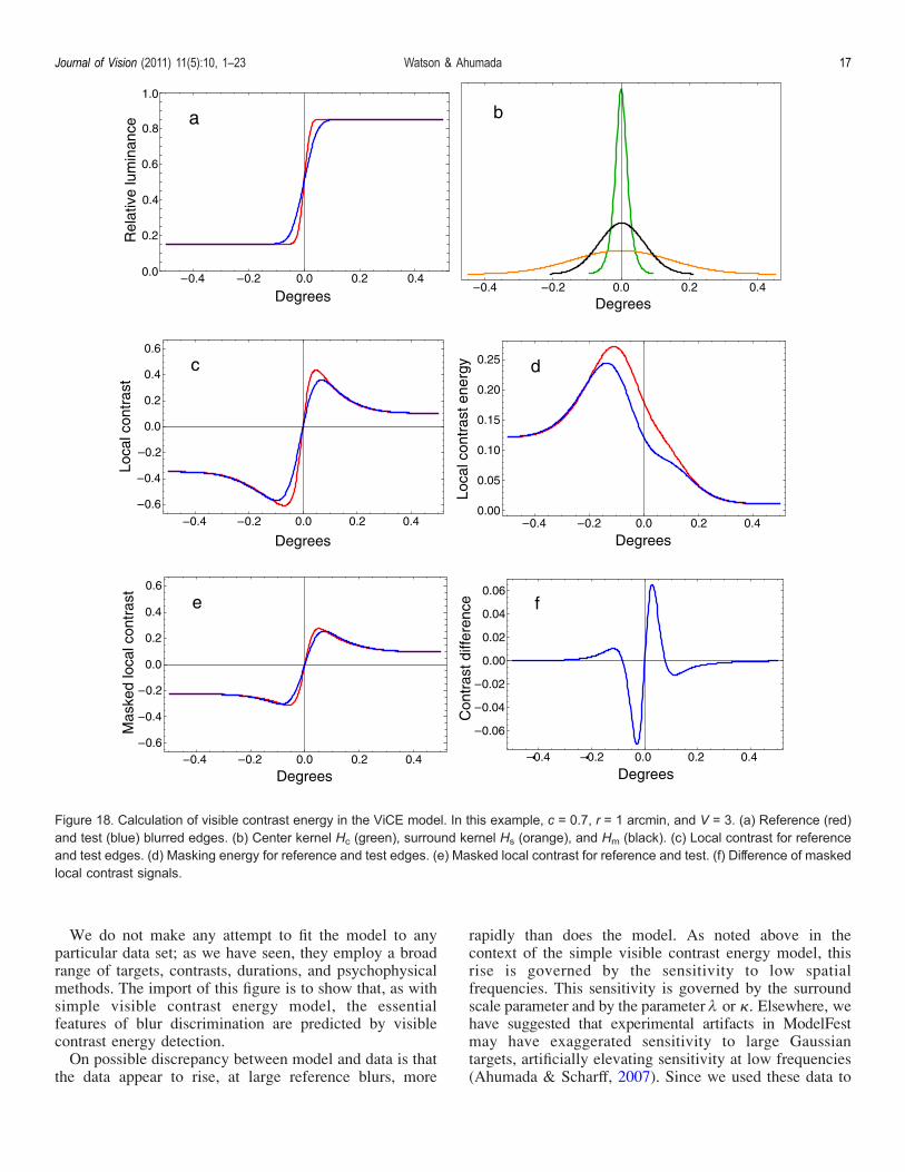
where + is a gain parameter, Hp is a Gaussian poolingkernel with scale % (in degrees), and px is the width of onewaveform sample in degrees (this assumes a discretesampled representation of the waveforms). The poolingkernel determines the area over which the energy ispooled. Based loosely on estimates from similar models fitto the ModelFest data, we set % = 1 deg. The Max operatorreturns the maximum of a waveform. Several of the stepsinvolved in this model are illustrated in Figure 18.While appearing rather different, this is in fact quite

close to the simple model discussed earlier. The primarydifferences were noted above. One additional difference isthat here we take the square root of the energy. Sincethreshold is defined as when this quantity equals 1, thisdifference has no practical import.To determine the parameters of this model, we again

make use of the ModelFest Gabor data discussed above(Figure 14). We obtain predictions using the one-dimensional profile of the Gabor as the luminance waveformfor l1 and a constant waveform of the backgroundluminance to create l2. The result of this fit is shown inFigure 19. The estimated parameters are 7 = 2.766 arcmin,E = 21.6 arcmin, + = 217.65, and . = 0.772. Note that inthis case (unlike Figure 14) we make use of the highestfrequency Gabor and that the fit is considerably better,showing that the hyperbolic secant function is a muchbetter representation of the center mechanism than theGaussian.Watson and Ahumada (2005) also fit a visible contrast

energy model employing a hyperbolic secant (sech) minusa Gaussian CSF to the complete set of ModelFest stimuliand published parameter estimates (line 13 of Table 5).Converting to scales, their estimates were7 = 2.758 arcmin,E = 18.76 arcmin, 1 = 0.78, and + = 329.9. The values aresimilar to those obtained here, but the gain is larger.However, the model in Watson and Ahumada was two-dimensional and included a Gaussian spatial aperture, anoblique effect, and two-dimensional CSF, all of whichwould entail a larger gain.With these parameters, we are now able to simulate the

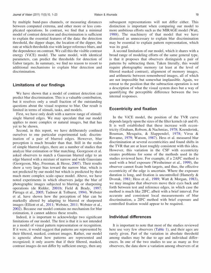
TVR curve and the effect of contrast. The TVR curve forthe model and a stimulus of 0.2 contrast is shown inFigure 20. As with the simple model discussed earlier, wesee that the visible contrast energy model predicts theessential features of the TVR curve: the absolute thresh-old, the dipper, the location of the dipper, and the rise withlarger reference blurs.


We do not make any attempt to fit the model to anyparticular data set; as we have seen, they employ a broadrange of targets, contrasts, durations, and psychophysicalmethods. The import of this figure is to show that, as withsimple visible contrast energy model, the essentialfeatures of blur discrimination are predicted by visiblecontrast energy detection.On possible discrepancy between model and data is that

the data appear to rise, at large reference blurs, more

rapidly than does the model. As noted above in thecontext of the simple visible contrast energy model, thisrise is governed by the sensitivity to low spatialfrequencies. This sensitivity is governed by the surroundscale parameter and by the parameter 1 or .. Elsewhere, wehave suggested that experimental artifacts in ModelFestmay have exaggerated sensitivity to large Gaussiantargets, artificially elevating sensitivity at low frequencies(Ahumada & Scharff, 2007). Since we used these data to

Figure 18. Calculation of visible contrast energy in the ViCE model. In this example, c = 0.7, r = 1 arcmin, and V = 3. (a) Reference (red)and test (blue) blurred edges. (b) Center kernel Hc (green), surround kernel Hs (orange), and Hm (black). (c) Local contrast for referenceand test edges. (d) Masking energy for reference and test edges. (e) Masked local contrast for reference and test. (f) Difference of maskedlocal contrast signals.


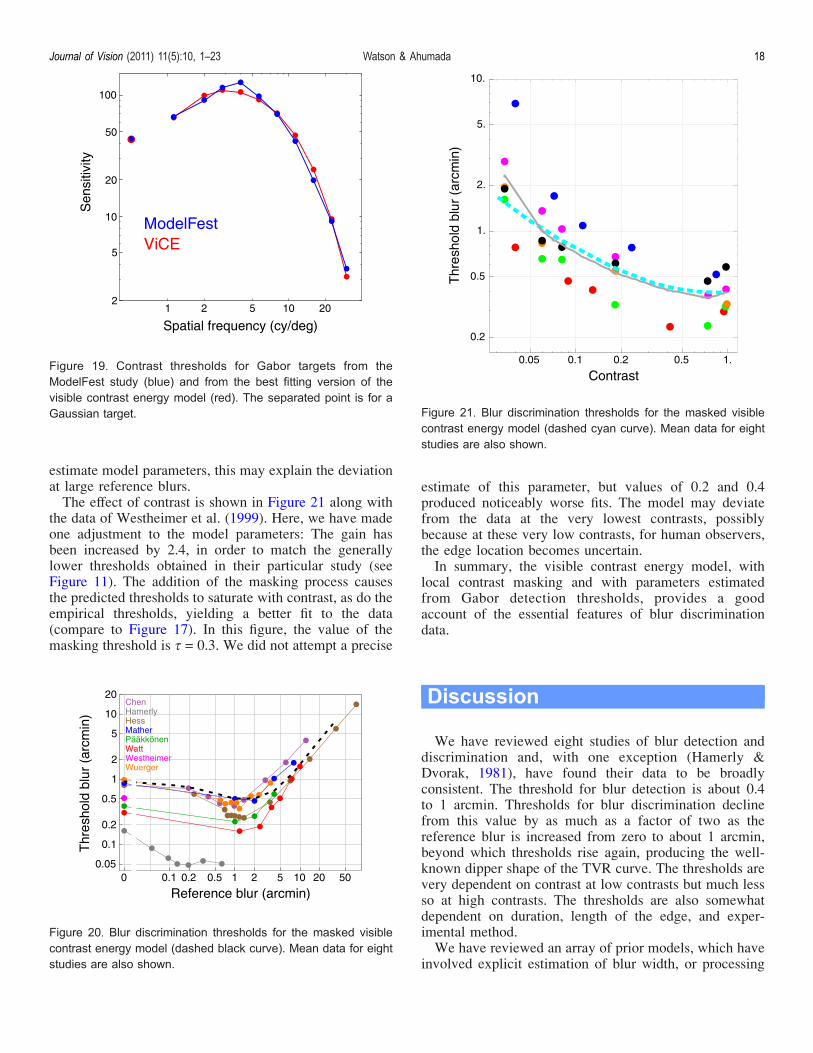
estimate model parameters, this may explain the deviationat large reference blurs.The effect of contrast is shown in Figure 21 along with

the data of Westheimer et al. (1999). Here, we have madeone adjustment to the model parameters: The gain hasbeen increased by 2.4, in order to match the generallylower thresholds obtained in their particular study (seeFigure 11). The addition of the masking process causesthe predicted thresholds to saturate with contrast, as do theempirical thresholds, yielding a better fit to the data(compare to Figure 17). In this figure, the value of themasking threshold is C = 0.3. We did not attempt a precise

estimate of this parameter, but values of 0.2 and 0.4produced noticeably worse fits. The model may deviatefrom the data at the very lowest contrasts, possiblybecause at these very low contrasts, for human observers,the edge location becomes uncertain.In summary, the visible contrast energy model, with

local contrast masking and with parameters estimatedfrom Gabor detection thresholds, provides a goodaccount of the essential features of blur discriminationdata.

Discussion

We have reviewed eight studies of blur detection anddiscrimination and, with one exception (Hamerly &Dvorak, 1981), have found their data to be broadlyconsistent. The threshold for blur detection is about 0.4to 1 arcmin. Thresholds for blur discrimination declinefrom this value by as much as a factor of two as thereference blur is increased from zero to about 1 arcmin,beyond which thresholds rise again, producing the well-known dipper shape of the TVR curve. The thresholds arevery dependent on contrast at low contrasts but much lessso at high contrasts. The thresholds are also somewhatdependent on duration, length of the edge, and exper-imental method.We have reviewed an array of prior models, which have

involved explicit estimation of blur width, or processing

Figure 19. Contrast thresholds for Gabor targets from theModelFest study (blue) and from the best fitting version of thevisible contrast energy model (red). The separated point is for aGaussian target.

Figure 20. Blur discrimination thresholds for the masked visiblecontrast energy model (dashed black curve). Mean data for eightstudies are also shown.

Figure 21. Blur discrimination thresholds for the masked visiblecontrast energy model (dashed cyan curve). Mean data for eightstudies are also shown.


by multiple band-pass channels, or measuring distancesbetween computed extrema, and other more or less com-plicated operations. In contrast, we find that a minimalmodel of contrast detection and discrimination is sufficientto explain the essential features of the data: the detectionthreshold, the dipper shape, the location of the dipper, therate at which thresholds rise with larger reference blurs, andthe dependence on contrast. We call this the visible contrastenergy (ViCE) model. The same model, with identicalparameters, can predict the thresholds for detection ofGabor targets. In summary, we find no reason to resort toadditional mechanisms to explain blur detection anddiscrimination.

Limitations of our findings

We have shown that a model of contrast detection canpredict blur discrimination. This is a valuable contribution,but it resolves only a small fraction of the outstandingquestions about the visual response to blur. Our result islimited in terms of stimuli, tasks, and models.First, we have only dealt with a narrow range of stimuli:

single blurred edges. We may speculate that our modelapplies to more complex or natural images, but that hasyet to be shown.Second, in this report, we have deliberately confined

ourselves to one particular experimental task: discrim-ination of a pair of blurred edges. However, blurperception is much broader than that. Still in the realmof simple blurred edges, there are a number of studies thatanalyze blur estimation or blur matching. Georgeson et al.asked observers to match a Gaussian blurred edge to anedge blurred with a mixture of narrow and wide Gaussians(Georgeson, May, Freeman, & Hesse, 2007). Their resultsshow a very large bias toward the narrow blur, which isnot predicted by our model but which is predicted by theirmuch more complex scale–space model. Above, we havenoted experiments in which observers judge the blur ofphotographic images subjected to blurring or sharpeningoperations (de Ridder, 2001b; Field & Brady, 1997;Parraga et al., 2005; Tadmor & Tolhurst, 1994). Websteret al. have shown how the perception of blur can bemarkedly altered by adapting to blurred or sharpenedimages (Elliott et al., 2011; Webster, 2011; Webster et al.,2002). Because our model contains no mechanism for blurestimation, it cannot address these results.Indeed, it is important to acknowledge two significant

limitations of our model. The first is that it is not intendedas a model of visual pattern representation or recognition.If it were, it would suggest that patterns are represented bytheir filtered, masked, contrast images. Rather, our modelis agnostic about how patterns are represented andrecognized; it only asserts that if their filtered, masked,contrast images do not differ by sufficient energy, then any

subsequent representations will not differ either. Thisdistinction is important when comparing our model tomore ambitious efforts such as the MIRAGE model (Watt,1988). The machinery of that model that we havedismissed as unnecessary to explain blur discriminationmay be essential to explain pattern representation, whichwas its goal.A second limitation of our model, which it shares with a

broad range of modeling efforts of the same general type,is that it proposes that observers distinguish a pair ofpatterns by subtracting them. Taken literally, this wouldrequire photographic memory (at least at the level offiltered masked contrast), alignment of memory images,and arithmetic between remembered images, all of whichare not impossible but somewhat implausible. Again, weretreat to the position that the subtraction operation is nota description of what the visual system does but a way ofquantifying the perceptible difference between the twointernal responses.

Eccentricity and fixation

In the ViCE model, the position of the TVR curvedepends largely upon the sizes of the filter kernels (7 and E).It is well established that these increase with eccen-tricity (Graham, Robson, & Nachmias, 1978; Koenderink,Bouman, Mesquita, & Slappendel, 1978; Virsu &Rovamo, 1979; Watson, 1987). Hess et al. measured blurdiscrimination at several eccentricities and found shifts inthe TVR that are at least roughly consistent with this idea.However, this variation in the CSF with eccentricitycreates problems for some of the methods used in thestudies reviewed here. For example, if a 2AFC method isused with a brief exposure (Westheimer et al., 1999), theobserver cannot fixate both targets, and thus, the effectiveeccentricity of the edge is uncertain. Where the exposureduration is long, and fixation is uncontrolled (Hamerly &Dvorak, 1981; Hess et al., 1989; Watt & Morgan, 1983),we may imagine that observers move their eyes back andforth between test and reference edges, in which case themethod is much like 2IFC, albeit with a brief interval. Foraccurate and consistent local measurements of blurdiscrimination, a 2IFC method with brief exposure andcontrolled fixation would appear to be required.

Individual differences

It is important to note that most of the studies reviewedhere use very few observers (Table 1), and their ages arerarely given. Part of the variation in absolute thresholdamong studies may be due to age and individual differ-ences. In one of the two studies to use as many as fiveobservers, the data show a variation among observers of at


least a factor of 2 (Westheimer et al., 1999). The twoobservers of Hamerly and Dvorak (1981) differ by anoverall factor of 2.6. In the ViCE model, the blurdetection threshold depends largely on the parameter 7,which also determines sensitivity at high spatial frequen-cies and acuity. Thresholds, in general, depend upon thegain parameter + , which is analogous to peak contrastsensitivity. In this regard, it is worth noting that bothcontrast sensitivity and acuity decline with age in adults.From 1920s to 1980s, in the absence of obvious ocularpathology, contrast sensitivity at 16 cycles/deg declines byabout 0.1 log unit per decade, while LogMAR acuitydeclines by 0.07 (Owsley, Sekuler, & Siemsen, 1983).Thus, we may expect substantial differences in blursensitivity between observers as a result of differences inacuity and contrast sensitivity.

Intrinsic blur

In our discussion of the Weber model, we have objectedto the introduction of the concept of “intrinsic blur,”regarding it as ad hoc and superfluous. In that model, it isan estimate of the blur that is inherent in visualprocessing. However, the ViCE model also has whatmight be considered an “intrinsic blur,” in the blurimposed by the center kernel. Our estimate for the widthof that kernel, when expressed as a Gaussian standarddeviation, is 0.98 arcmin, almost identical to the meanvalue of 0.97 arcmin that we estimate from the Webermodel (for > = 1, excluding Hamerly & Dvorak, in Table 2).While this quantitative agreement may be reassuring, themathematical reasons for it remain obscure, hidden inEquation 16. It should also be noted that the reasons forthe eventual rise in thresholds at large reference blurs arevery different for the two models. In the Weber model, itis because the model assumes that the discriminabledifference in perceived blur rises in proportion toperceived blur, while in the ViCE model it is due largelyto the attenuation of low spatial frequencies due to thesurround mechanism.

Optical blur

The center kernel Hc and its scale 7 play a central rolein the ViCE model in determining the sensitivity to blur.This kernel must incorporate any optical blur present inthe eye of the observer. Any additional blur forms what isknown as the neural transfer function (NTF). Sekiguchi,Williams, and Brainard (1993) estimated a very smalladditional blur, corresponding to an NTF represented by aGaussian with a scale of 0.75 arcmin. Recently, we haveargued that even this additional blur may be betterattributed to limits on spatial summation, themselves the

result of retinal inhomogeneity (Ahumada, Coletta, &Watson, 2010). Thus, most and perhaps all of the limits onblur discrimination, at least for small reference blurs, aredue to optical limitations. However, discrimination atlarge reference blurs depends upon the behavior of theCSF at low spatial frequencies (see Figure 16), which isnot optical in origin.

Conclusions

We have reviewed data from eight studies of blurdetection and discrimination in single edges. We findgood agreement among the studies, apart from discrep-ancies that may be due to methodological, stimulus, orobserver differences. We also find that the general patternof results and overall sensitivity are consistent with ageneral model in which observers discriminate betweentwo images when the energy of the difference betweentheir masked local contrast waveforms exceeds a thresh-old. We call this the visible contrast energy (ViCE)model. We conclude that blur detection and discrimina-tion are instances of contrast detection. We further notethat much of the limitation on blur discriminationperformance, for small reference blurs, is due to opticalblur.

Appendix A

Notation

In the following, we define the notation used in the text.Where available, we note default values of modelparameters. In the text, primed quantities representGaussian scales, converted from standard deviationsaccording to Equation 10.

Stimuli

Weber model

c Contrastr Standard deviation of reference Gaussian blur (deg)a Standard deviation of added Gaussian blur (deg)

" Standard deviation of internal Gaussian blur (deg)A Standard deviation of perceived Gaussian blur (deg)5 Weber constant> Weber exponent


Appendix B

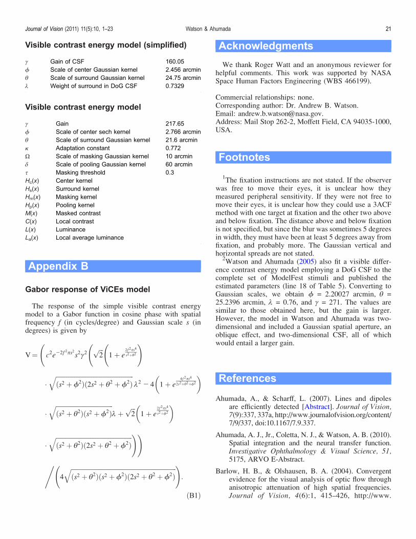
Gabor response of ViCEs model

The response of the simple visible contrast energymodel to a Gabor function in cosine phase with spatialfrequency f (in cycles/degree) and Gaussian scale s (indegrees) is given by

V¼ c2ej2f 2:s2s2+2

ffiffiffi2

p 1þ e

2 f2:s4

s2þE2

!

�ffiffiffiffiffiffiffiffiffiffiffiffiffiffiffiffiffiffiffiffiffiffiffiffiffiffiffiffiffiffiffiffiffiffiffiffiffiffiffiffiffiffiffiffiffiffiffiffiffiffiðs2 þ 72Þð2s2 þ E2 þ 72Þ

q12 j 4 1þ e

4 f2:s4

2s2þE2þ72

� �

�ffiffiffiffiffiffiffiffiffiffiffiffiffiffiffiffiffiffiffiffiffiffiffiffiffiffiffiffiffiffiffiffiffiffiffiffiffiðs2 þ E2Þðs2 þ 72Þ

q1þ

ffiffiffi2

p1þ e

2 f2:s4

s2þ72

� �

�ffiffiffiffiffiffiffiffiffiffiffiffiffiffiffiffiffiffiffiffiffiffiffiffiffiffiffiffiffiffiffiffiffiffiffiffiffiffiffiffiffiffiffiffiffiffiffiffiffiðs2 þ E2Þð2s2 þ E2 þ 72Þ

q !!

, 4

ffiffiffiffiffiffiffiffiffiffiffiffiffiffiffiffiffiffiffiffiffiffiffiffiffiffiffiffiffiffiffiffiffiffiffiffiffiffiffiffiffiffiffiffiffiffiffiffiffiffiffiffiffiffiffiffiffiffiffiffiffiffiffiffiffiffiffiffiðs2 þ E2Þðs2 þ 72Þð2s2 þ E2 þ 72Þ

q !:

ðB1Þ

Acknowledgments

We thank Roger Watt and an anonymous reviewer forhelpful comments. This work was supported by NASASpace Human Factors Engineering (WBS 466199).

Commercial relationships: none.Corresponding author: Dr. Andrew B. Watson.Email: [email protected]: Mail Stop 262-2, Moffett Field, CA 94035-1000,USA.

Footnotes

1The fixation instructions are not stated. If the observer

was free to move their eyes, it is unclear how theymeasured peripheral sensitivity. If they were not free tomove their eyes, it is unclear how they could use a 3ACFmethod with one target at fixation and the other two aboveand below fixation. The distance above and below fixationis not specified, but since the blur was sometimes 5 degreesin width, they must have been at least 5 degrees away fromfixation, and probably more. The Gaussian vertical andhorizontal spreads are not stated.

2Watson and Ahumada (2005) also fit a visible differ-

ence contrast energy model employing a DoG CSF to thecomplete set of ModelFest stimuli and published theestimated parameters (line 18 of Table 5). Converting toGaussian scales, we obtain 7 = 2.20027 arcmin, E =25.2396 arcmin, 1 = 0.76, and + = 271. The values aresimilar to those obtained here, but the gain is larger.However, the model in Watson and Ahumada was two-dimensional and included a Gaussian spatial aperture, anoblique effect, and two-dimensional CSF, all of whichwould entail a larger gain.

References

Ahumada, A., & Scharff, L. (2007). Lines and dipolesare efficiently detected [Abstract]. Journal of Vision,7(9):337, 337a, http://www.journalofvision.org/content/7/9/337, doi:10.1167/7.9.337.

Ahumada, A. J., Jr., Coletta, N. J., & Watson, A. B. (2010).Spatial integration and the neural transfer function.Investigative Ophthalmology & Visual Science, 51,5175, ARVO E-Abstract.

Barlow, H. B., & Olshausen, B. A. (2004). Convergentevidence for the visual analysis of optic flow throughanisotropic attenuation of high spatial frequencies.Journal of Vision, 4(6):1, 415–426, http://www.

+ Gain of CSF 160.057 Scale of center Gaussian kernel 2.456 arcminE Scale of surround Gaussian kernel 24.75 arcmin1 Weight of surround in DoG CSF 0.7329

+ Gain 217.657 Scale of center sech kernel 2.766 arcminE Scale of surround Gaussian kernel 21.6 arcmin. Adaptation constant 0.7724 Scale of masking Gaussian kernel 10 arcmin% Scale of pooling Gaussian kernel 60 arcminC Masking threshold 0.3Hc(x) Center kernelHs(x) Surround kernelHm(x) Masking kernelHp(x) Pooling kernelM(x) Masked contrastC(x) Local contrastL(x) LuminanceLa(x) Local average luminance

Visible contrast energy model (simplified)

Visible contrast energy model



journalofvision.org/content/4/6/1, doi:10.1167/4.6.1.[PubMed] [Article]

Burr, D. C., & Ross, J. (2002). Direct evidence that“speedlines” influence motion mechanisms. Journalof Neuroscience, 22, 8661–8664. [Article]

Campbell, F. W., & Westheimer, G. (1958). Sensitivity ofthe eye to differences in focus. The Journal ofPhysiology, 143, 18P. [Article]

Carney, T., Tyler, C. W., Watson, A. B., Makous, W.,Beutter, B., Chen, C.-C., et al. (2000). Modelfest:Year one results and plans for future years. HumanVision, Visual Processing, and Digital Display IX,3959, 140–151.

Chen, C.-C., Chen, K.-P., Tseng, C.-H., Kuo, S.-T., &Wu, K.-N. (2009). Constructing a metrics for blurperception with blur discrimination experiments.Paper presented at the Image Quality and SystemPerformance VI, San Jose, CA, USA, http://link.aip.org/link/%3FPSI/7242/724219/1.

de Ridder, H. (2001a). Cognitive issues in image qualitymeasurement. Journal of Electronic Imaging, 10, 47–55.

de Ridder, H. (2001b). Image processing and the problemof quantifying image quality. Paper presented at the2001 International Conference on Image Processing.

Elliott, S. L., Georgeson, M. A., & Webster, M. A. (2011).Response normalization and blur adaptation: Data andmulti-scale model. Journal of Vision, 11(2):7, 1–18,http://www.journalofvision.org/content/11/2/7,doi:10.1167/11.2.7. [PubMed] [Article]

Farrell, J., Xu, J., Larson, K., & Wandell, B. (2009).Visual preference for ClearType technology. Societyfor Information Display Digest of Technical Papers,2009, 702–705.

Ferzli, R., & Karam, L. J. (2006). Human visual systembased on no-reference objective image sharpnessmetric. Paper presented at the 2006 IEEE Interna-tional Conference on Image Processing, doi:10.1109/ICIP.2006.312925.

Field, D. J., & Brady, N. (1997). Visual sensitivity, blurand the sources of variability in the amplitude spectraof natural scenes. Vision Research, 37, 3367–3383,doi:10.1016/S0042-6989(97)00181-8. [Article]

Fiske, T. J., Silverstein, L. D., Hodgson, S., & Watson,A. B. (2007). Visual quality of high-contrast projectionscreens: Part I. Visibility of screen-based artifacts andnoise. Journal of the Society for Information Display,15, 409–419. [PubMed] [Article]

Geisler, W. S. (1999). Motion streaks provide a spatial codefor motion direction. Nature, 400, 65–69. [Article]

Georgeson, M. A., May, K. A., Freeman, T. C., & Hesse,G. S. (2007). From filters to features: Scale–

space analysis of edge and blur coding in humanvision. Journal of Vision, 7(13):7, 1–21, http://www.journalofvision.org/content/7/13/7, doi:10.1167/7.13.7. [PubMed] [Article]

Graham, N., Robson, J. G., & Nachmias, J. (1978). Gratingsummation in fovea and periphery. Vision Research, 18,815–825, doi:10.1016/0042-6989(78)90122-0. [Article]

Granger, E. M., & Cupery, K. N. (1972). An optical meritfunction (SQF) which correlates with subjective imagejudgements. Photographic Science and Engineering,16, 221–230.

Hamerly, J. R., & Dvorak, C. A. (1981). Detection anddiscrimination of blur in edges and lines. Journal ofthe Optical Society of America, 71, 448, doi:10.1364/JOSA.71.000448.

Harrington, T. L., & Harrington, M. K. (1981). Perceptionof motion using blur pattern information in themoderate and high-velocity domains of vision. ActaPsychologica, 48, 227–237. [Article]

Heeger, D. J. (1992). Normalization of cell responses incat striate cortex. Visual Neuroscience, 9, 181–197,doi:10.1017/S0952523800009640.

Held, R. T., Cooper, E. A., O’Brien, J. F., & Banks, M. S.(2010). Using blur to affect perceived distance and size.ACM Transactions on Graphics, 29, 1–16. [Article]

Hess, R. F., Pointer, J. S., & Watt, R. J. (1989). How arespatial filters used in fovea and parafovea? Journal ofthe Optical Society of America A, 6, 329. [Article]

Kayargadde, V., & Martens, J. B. (1996). Perceptual char-acterization of images degraded by blur and noise:Model. Journal of the Optical Society of America A:Optics, Image Science, and Vision, 13, 1178–1188,doi:10.1364/JOSAA.13.001166. [PubMed]

Koenderink, J. J., Bouman, M. A., Mesquita, A. E. B. d.,& Slappendel, S. (1978). Perimetry of contrastdetection thresholds of moving spatial sine wavepatterns: I. The near peripheral visual field (eccen-tricity 0-–8-). Journal of the Optical Society ofAmerica, 68, 845–849, doi:10.1364/JOSA.68.000845.

Kruger, P. B., & Pola, J. (1986). Stimuli for accommodation:Blur, chromatic aberration and size. Vision Research,26, 957–971, doi:10.1016/0042-6989(86)90153-7.[Article]

Legras, R., Chateau, N., & Charman, W. N. (2004).Assessment of just-noticeable differences for refractiveerrors and spherical aberration using visual simulation.Optometry & Vision Science, 81, 718–728. [Article]

Mather, G., & Smith, D. R. (2002). Blur discriminationand its relation to blur-mediated depth perception.Perception, 31, 1211–1219, doi:10.1068/p3254.[PubMed]


http://www.ncbi.nlm.nih.gov/entrez/query.fcgi?cmd=Retrieve&db=PubMed&dopt=Citation&list_uids=15330709


http://www.jneurosci.org/cgi/content/abstract/22/19/8661

http://jp.physoc.org/content/143/supplement/1P.full.pdftml

http://link.aip.org/link/%3FPSI/7242/724219/1

http://link.aip.org/link/%3FPSI/7242/724219/1

http://www.ncbi.nlm.nih.gov/pubmed/21307174


http://www.sciencedirect.com/science/article/pii/S0042698997001818

http://scitation.aip.org/getabs/servlet/GetabsServlet?prog=normal&id=JSIDE8000015000006000409000001

http://dx.doi.org/10.1889/1.2749327

http://dx.doi.org/10.1038/21886



http://www.sciencedirect.com/science/article/pii/0042698978901220

http://www.sciencedirect.com/science/article/B6V5T-45Y6NTH-V/2/6adae2c18a338a4d2366dc972834cc77

http://doi.acm.org/10.1145/1731047.1731057

http://josaa.osa.org/abstract.cfm?URI=josaa-6-2-329


http://www.sciencedirect.com/science/article/B6T0W-484M9JS-24Y/2/8c9f1ed4367b0dc82b8e13579c6cd774

http://journals.lww.com/optvissci/Fulltext/2004/09000/Assessment_of_Just_Noticeable_Differences_for.17.aspx


Owsley, C., Sekuler, R., & Siemsen, D. (1983). Contrastsensitivity throughout adulthood. Vision Research,23, 689–699, doi:10.1016/0042-6989(83)90210-9.[PubMed] [Article]

Paakkonen, A. K., & Morgan, M. J. (1994). Effectsof motion on blur discrimination. Journal of theOptical Society of America A, 11, 992, doi:10.1364/JOSAA.11.000992.

Parraga, C. A., Troscianko, T., & Tolhurst, D. J. (2005).The effects of amplitude-spectrum statistics on fovealand peripheral discrimination of changes in naturalimages, and a multi-resolution model. VisionResearch, 45, 3145–3168. [Article]

Rohaly, A. M., Ahumada, A. J., Jr., & Watson, A. B.(1997). Object detection in natural backgroundspredicted by discrimination performance and models.Vision Research, 37, 3225–3235, doi:10.1016/S0042-6989(97)00156-9. [Article]

Sekiguchi, N., Williams, D. R., & Brainard, D. H. (1993).Efficiency in detection of isoluminant and isochromaticinterference fringes. Journal of the Optical Societyof America A, 10, 2118–2133, doi:10.1364/JOSAA.10.002118.

Tadmor, Y., & Tolhurst, D. J. (1994). Discrimination ofchanges in the second-order statistics of natural andsynthetic images. Vision Research, 34, 541–554.[Article]

Thibos, L. N. (2009). Retinal image quality for virtual eyesgenerated by a statistical model of ocular wavefrontaberrations. Ophthalmic & Physiological Optics, 29,288–291, doi:10.1111/j.1475-1313.2009.00662.x.[PubMed]

Thibos, L. N., Hong, X., Bradley, A., & Cheng, X. (2002).Statistical variation of aberration structure and imagequality in a normal population of healthy eyes. Journalof the Optical Society of America A: Optics, ImageScience, and Vision, 19, 2329–2348. [Article]

Virsu, V., & Rovamo, J. (1979). Visual resolution, contrastsensitivity, and the cortical magnification factor.Experimental Brain Research, 37, 475–494,doi:10.1007/BF00236818. [Article]

Walsh, G., & Charman, W. N. (1988). Visual sensitivityto temporal change in focus and its relevance to theaccommodation response. Vision Research, 28,1207–1221, doi:10.1016/0042-6989(88)90037-5.[Article]

Wang, B., & Ciuffreda, K. J. (2005). Foveal blur discrim-ination of the human eye.Ophthalmic & PhysiologicalOptics, 25, 45–51, doi:10.1111/j.1475-1313.2004.00250.x. [PubMed]

Watson, A. B. (1987). Estimation of local spatialscale. Journal of the Optical Society of America A, 4,1579–1582, doi:10.1364/JOSAA.4.001579.

Watson, A. B. (2010a). Display motion blur: Comparisonof measurement methods. Journal of the Society forInformation Display, 18, 179–190, doi:10.1089/JSID18.2.179. [Article]

Watson, A. B. (2010b). Visible motion blur: A perceptualmetric for display motion blur. Society for InformationDisplay Digest of Technical Papers, 41, 184–187.

Watson, A. B., & Ahumada, A. J., Jr. (2005). A standardmodel for foveal detection of spatial contrast.Journal of Vision, 5(9):6, 717–740, http://www.journalofvision.org/content/5/9/6, doi:10.1167/5.9.6.[PubMed] [Article]

Watson, A. B., & Ahumada, A. J., Jr. (2008). Predictingvisual acuity from wavefront aberrations. Journal ofVision, 8(4):17, 1–19, http://www.journalofvision.org/content/8/4/17, doi:10.1167/8.4.17. [PubMed] [Article]

Watson, A. B., & Solomon, J. A. (1997). Model of visualcontrast gain control and pattern masking. Journal ofthe Optical Society of America A: Optics, ImageScience, and Vision, 14, 2379–2391, doi:10.1364/JOSAA.14.002379.

Watt, R. J. (1988). Visual processing: Computational,psychophysical, and cognitive research. Hove, UK;Hillsdale, NJ: L. Erlbaum Associates.

Watt, R. J., & Morgan, M. J. (1983). The recognition andrepresentation of edge blur: Evidence for spatialprimitives in human vision. Vision Research, 23,1465–1477, doi:10.1016/0042-6989(83)90158-X.[Article]

Watt, R. J., & Morgan, M. J. (1984). Spatial filters and thelocalization of luminance changes in human vision.Vision Research, 24, 1387–1397, doi:10.1016/0042-6989(84)90194-9. [PubMed] [Article]

Webster, M. A. (2011). Adaptation and visualcoding. Journal of Vision, 11(5):3, 1–23, http://www.journalofvision.org/content/11/5/3, doi:10.1167/11.5.3.[PubMed] [Article]

Webster, M. A., Georgeson, M. A., & Webster, S. M.(2002). Neural adjustments to image blur. NatureNeuroscience, 5, 839–840, doi:10.1038/nn906.[PubMed]

Westheimer, G., Brincat, S., & Wehrhahn, C. (1999).Contrast dependency of foveal spatial functions:Orientation, vernier, separation, blur and displace-ment discrimination and the tilt and Poggendorffillusions. Vision Research, 39, 1631–1639. [Article]

Wuerger, S. M., Owens, H., & Westland, S. (2001). Blurtolerance for luminance and chromatic stimuli. Journalof the Optical Society of America A, 18, 1231–1239,doi:10.1364/JOSAA.18.001231.




http://www.sciencedirect.com/science/article/B6T0W-4H5DY6H-1/2/313cacec2da66ea710e9a3f6c2bd1796

http://www.sciencedirect.com/science/article/pii/S0042698997001569

http://www.sciencedirect.com/science/article/B6T0W-4835PK8-73/2/04fccd3f729a6d0deed73c8e81294e63


http://josaa.osa.org/abstract.cfm?URI=josaa-19-12-2329

http://www.mendeley.com/research/visual-resolution-contrast-sensitivity-and-the-cortical-magnification-factor/

http://www.sciencedirect.com/science/article/B6T0W-484DYV0-19W/2/851ecdc131358aa1525de1a48087f867


http://ntrs.nasa.gov/archive/nasa/casi.ntrs.nasa.gov/20110003569_2011001040.pdf





http://www.sciencedirect.com/science/article/pii/004269898390158X






http://www.sciencedirect.com/science/article/B6T0W-3VNPJ5G-M/2/8f6482b60a3776335468927536984ed9

Documents

Blur clariﬁed: A review and synthesis of blur discrimination