BOILING WATER REACTOR TURBINE TRIP (TT) BENCHMARK€¦ · · 2005-08-12BOILING WATER REACTOR TURBINE TRIP (TT) ... sponsorship a PWR main steam line break (MSLB) benchmark against

ISBN 92-64-01064-5 NEA/NSC/DOC(2004)21

NEA NUCLEAR SCIENCE COMMITTEE NEA COMMITTEE ON SAFETY OF NUCLEAR INSTALLATIONS

BOILING WATER REACTOR TURBINE TRIP (TT) BENCHMARK

Volume II: Summary Results of Exercise 1

June 2005

by

Bedirhan Akdeniz and Kostadin N. Ivanov Nuclear Engineering Program

The Pennsylvania State University University Park, PA, 16802 USA

Andy M. Olson Exelon Nuclear

200 Exelon Way, KSA2-N Kennett Square, PA, 19348 USA

© OECD 2005 NEA No. 4448

NUCLEAR ENERGY AGENCY ORGANISATION FOR ECONOMIC CO-OPERATION AND DEVELOPMENT

AND US NUCLEAR REGULATORY COMMISSION

ORGANISATION FOR ECONOMIC CO-OPERATION AND DEVELOPMENT

The OECD is a unique forum where the governments of 30 democracies work together to address the economic, social and environmental challenges of globalisation. The OECD is also at the forefront of efforts to understand and to help governments respond to new developments and concerns, such as corporate governance, the information economy and the challenges of an ageing population. The Organisation provides a setting where governments can compare policy experiences, seek answers to common problems, identify good practice and work to co-ordinate domestic and international policies.

The OECD member countries are: Australia, Austria, Belgium, Canada, the Czech Republic, Denmark, Finland, France, Germany, Greece, Hungary, Iceland, Ireland, Italy, Japan, Korea, Luxembourg, Mexico, the Netherlands, New Zealand, Norway, Poland, Portugal, the Slovak Republic, Spain, Sweden, Switzerland, Turkey, the United Kingdom and the United States. The Commission of the European Communities takes part in the work of the OECD.

OECD Publishing disseminates widely the results of the Organisation’s statistics gathering and research on economic, social and environmental issues, as well as the conventions, guidelines and standards agreed by its members.

* * *

This work is published on the responsibility of the Secretary-General of the OECD. The opinions expressed and arguments employed herein do not necessarily reflect the official views of the Organisation or of the governments of its member countries.

NUCLEAR ENERGY AGENCY

The OECD Nuclear Energy Agency (NEA) was established on 1st February 1958 under the name of the OEEC European Nuclear Energy Agency. It received its present designation on 20th April 1972, when Japan became its first non-European full member. NEA membership today consists of 28 OECD member countries: Australia, Austria, Belgium, Canada, the Czech Republic, Denmark, Finland, France, Germany, Greece, Hungary, Iceland, Ireland, Italy, Japan, Luxembourg, Mexico, the Netherlands, Norway, Portugal, Republic of Korea, the Slovak Republic, Spain, Sweden, Switzerland, Turkey, the United Kingdom and the United States. The Commission of the European Communities also takes part in the work of the Agency.

The mission of the NEA is:

� to assist its member countries in maintaining and further developing, through international co-operation, the scientific, technological and legal bases required for a safe, environmentally friendly and economical use of nuclear energy for peaceful purposes, as well as

� to provide authoritative assessments and to forge common understandings on key issues, as input to government decisions on nuclear energy policy and to broader OECD policy analyses in areas such as energy and sustainable development.

Specific areas of competence of the NEA include safety and regulation of nuclear activities, radioactive waste management, radiological protection, nuclear science, economic and technical analyses of the nuclear fuel cycle, nuclear law and liability, and public information. The NEA Data Bank provides nuclear data and computer program services for participating countries.

In these and related tasks, the NEA works in close collaboration with the International Atomic Energy Agency in Vienna, with which it has a Co-operation Agreement, as well as with other international organisations in the nuclear field.

© OECD 2005 No reproduction, copy, transmission or translation of this publication may be made without written permission. Applications should be sent to OECD Publishing: [email protected] or by fax (+33-1) 45 24 13 91. Permission to photocopy a portion of this work should be addressed to the Centre Français d’exploitation du droit de Copie, 20 rue des Grands Augustins, 75006 Paris, France ([email protected]).

3

FOREWORD

The OECD Nuclear Energy Agency (NEA) completed under US Nuclear Regulatory Commission (NRC) sponsorship a PWR main steam line break (MSLB) benchmark against coupled system three-dimensional (3-D) neutron kinetics and thermal-hydraulic codes. Another OECD/NRC coupled-code benchmark was recently completed for a BWR turbine trip (TT) transient and is the object of the present report.

Turbine trip transients in a BWR are pressurisation events in which the coupling between core space-dependent neutronic phenomena and system dynamics plays an important role. The data made available from actual experiments carried out at the Peach Bottom 2 plant make the present benchmark particularly valuable. While defining and co-ordinating the BWR TT benchmark, a systematic approach and level methodology not only allowed for a consistent and comprehensive validation process, but also contributed to the study of key parameters of pressurisation transients. The benchmark consists of three separate exercises, two initial states and five transient scenarios.

The BWR TT Benchmark will be published in four volumes as NEA reports. CD-ROMs will also be prepared and will include the four reports and the transient boundary conditions, decay heat values as a function of time, cross-section libraries and supplementary tables and graphs not published in the paper version. BWR TT Benchmark – Volume I: Final Specifications was issued in 2001 [NEA/NSC/DOC(2001)1]. The benchmark team [Pennsylvania State University (PSU) in co-operation with Exelon Nuclear and the NEA] has been responsible for co-ordinating benchmark activities, answering participant questions and assisting them in developing their models, as well as analysing submitted solutions and providing reports summarising the results for each phase. The benchmark team has also been involved in the technical aspects of the benchmark, including sensitivity studies for the different exercises. In performing these tasks, the PSU team has been collaborating with Andy M. Olson and Kenneth W. Hunt of Exelon Nuclear. Lance J. Agee, of the Electric Power Research Institute (EPRI), has also provided technical assistance for this international benchmark project.

Volume II summarises the results for Exercise 1 of the benchmark and identifies the key parameters and important issues concerning the thermal-hydraulic system modelling of the TT transient with specified core average axial power distribution and fission power (or reactivity) time transient history. Exercise 1 helped the participants initialise and test their system code models for further use in Exercise 3 on coupled 3-D kinetics/system thermal-hydraulics simulations.

Readers are invited to note that many of the original graphics in the report are in colour; colour versions are available online at the NEA website (www.nea.fr).

4

Acknowledgements

The authors would like to thank Professor J. Aragonés of UPM, Dr. T. Lefvert and Dr. S. Langenbuch of GRS, and Dr. F. Eltawila of NRC, whose support and encouragement in establishing this benchmark were invaluable.

This report is the sum of many efforts – the participants and the funding agencies and their staff, including the US Nuclear Regulatory Commission and the Organisation of Economic Co-operation and Development. Special appreciation is due to: L. Agee of EPRI, Professor T. Downar of Purdue University, B. Aktas of ISL Inc., Dr. G. Gose and Dr. C. Peterson from CSA, Dr. A. Hotta of TSI, Dr. P. Coddington of PSI and Dr. U. Grundmann of FZR. Their technical assistance, comments and suggestions were very valuable. We would like to thank them for the effort and time involved.

Of particular note are the labours of Dr. F. Eltawila, assisted by Dr. J. Han and Dr. J. Uhle of the US Nuclear Regulatory Commission. Through their endeavours, funding was secured for this project. We also thank them for their invaluable technical advice and assistance.

The authors wish to express their sincere appreciation for the outstanding support offered by Dr. E. Sartori, who provides efficient administration, organisation and valuable technical advice.

The authors would also like to particularly thank all of the OECD/NEA BWR Turbine Trip Benchmark participants for their valuable support, comment and feedback during this study.

Special thanks are due to the authors’ family members for their encouragement, support and patience throughout the course of this work.

Finally, the authors are grateful to A. Griffin-Chahid for having devoted her competence and skills to the editing of this report.

5

TABLE OF CONTENTS

Foreword ........................................................................................................................................ 3

List of Figures ................................................................................................................................ 7

List of Tables.................................................................................................................................. 9

List of Abbreviations ..................................................................................................................... 11

Chapter 1 INTRODUCTION..................................................................................................... 13

Chapter 2 DESCRIPTION OF EXERCISE 1 .......................................................................... 15

2.1 General ................................................................................................................ 15

2.2 Description of turbine trip scenario..................................................................... 15

2.3 Initial steady state conditions .............................................................................. 16

2.4 Transient calculations.......................................................................................... 18

Chapter 3 METHODOLOGIES FOR COMPARATIVE ANALYSIS.................................. 19

3.1 Standard techniques for the comparison of results.............................................. 19

3.1.1 Integral parameter values.......................................................................... 19

3.1.2 One-dimensional (1-D) axial distributions ............................................... 20

3.1.3 Time histories............................................................................................ 20

3.2 ACAP analysis .................................................................................................... 21

Chapter 4 RESULTS AND DISCUSSION OF EXERCISE 1 ................................................ 27

Chapter 5 CONCLUSIONS ....................................................................................................... 65

References ...................................................................................................................................... 67

Appendix A Description of computer codes used for analysis of Exercise 1 of the NEA-NRC BWR TT Benchmark................................................................... 69

CATHARE (CEA, France)....................................................................................... 71

S-RELAP5 (FANP, Germany) ................................................................................. 73

ATHLET (GRS, Germany) ...................................................................................... 73

DNB/3D (NETCORP, USA).................................................................................... 73

TRAC-BF1 (NFI, Japan).......................................................................................... 74

6

TRAC-BF1 (NUPEC, Japan) ................................................................................... 74

RETRAN-3D (PSI, Switzerland) ............................................................................. 74

TRAC-BF1/MOD1 (PSU, USA).............................................................................. 75

TRAC-M (PSU/NRC, USA) .................................................................................... 77

TRAC-BF1-ENTRÉE (TEPSYS, Japan) ................................................................. 78

RELAP5 (UPISA, Italy)........................................................................................... 80

TRAC-BF1-VALKIN (UPV, Spain)........................................................................ 80

POLCA-T (Westinghouse, Sweden) ........................................................................ 81

Appendix B Questionnaire for Exercise 1 of the NEA-NRC BWR TT Benchmark.................... 85

CATHARE2 v1.5 (CEA, France)............................................................................. 88

S-RELAP5 (FANP, Germany) ................................................................................. 91

ATHLET (GRS, Germany) ...................................................................................... 94

DNB/3D (NETCORP, USA).................................................................................... 97

TRAC-BF1 (NFI, Japan).......................................................................................... 103

TRAC-BF1 (NUPEC, Japan) ................................................................................... 106

RETRAN-3D (PSI, Switzerland) ............................................................................. 109

TRAC-BF1 (PSU, USA) .......................................................................................... 116

TRAC-M (PSU/NRC, USA) .................................................................................... 118

TRAC-BF1 (TEPSYS, Japan).................................................................................. 121

RELAP5 (UPISA, Italy)........................................................................................... 123

TRAC-BF1-VALKIN (UPV, Spain)........................................................................ 127

POLCA-T (Westinghouse, Sweden) ........................................................................ 130

7

List of Figures

Figure 2.3-1. PB2 TT2 initial core axial average power distribution from P1 edit ..................... 17

Figure 3.2-1. FOM configuration in ACAP ................................................................................ 22

Figure 4-1. Core inlet enthalpy................................................................................................. 30

Figure 4-2. Core pressure drop................................................................................................. 31

Figure 4-3. Core average void fraction distribution ................................................................. 32

Figure 4-4. Core average void fraction distribution ................................................................. 32

Figure 4-5. Void fraction distribution – averaged vs. Exelon data........................................... 33

Figure 4-6. Void fraction distribution – Exelon and deviation................................................. 33

Figure 4-7. Vessel dome pressure (5 seconds) ......................................................................... 36

Figure 4-8. Vessel dome pressure (5 seconds) ......................................................................... 36

Figure 4-9. Vessel dome pressure – measured vs. averaged data (5 seconds) ......................... 37

Figure 4-10. Vessel dome pressure (1.5 seconds) ...................................................................... 38

Figure 4-11. Vessel dome pressure (1.5 seconds) ...................................................................... 38

Figure 4-12. Vessel dome pressure – measured vs. averaged data (1.5 seconds) ...................... 39

Figure 4-13. Core exit pressure (5 seconds) ............................................................................... 40

Figure 4-14. Core exit pressure (5 seconds) ............................................................................... 40

Figure 4-15. Core exit pressure – Exelon vs. averaged data (5 seconds) ................................... 41

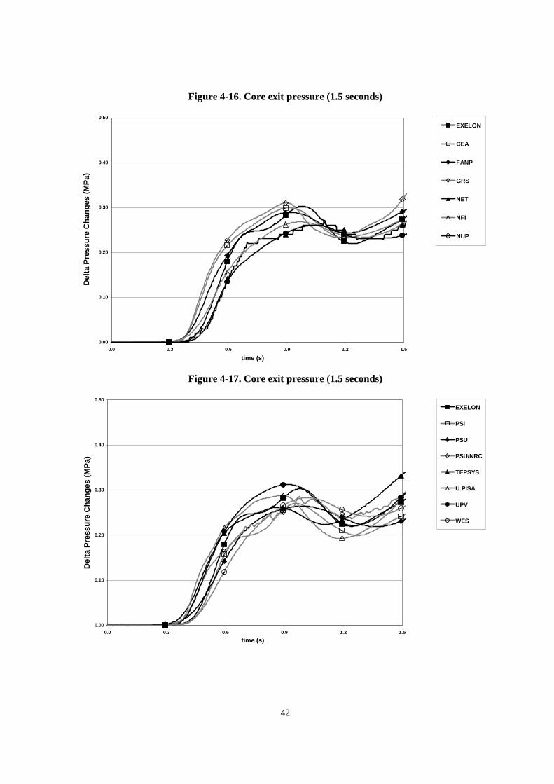
Figure 4-16. Core exit pressure (1.5 seconds) ............................................................................ 42

Figure 4-17. Core exit pressure (1.5 seconds) ............................................................................ 42

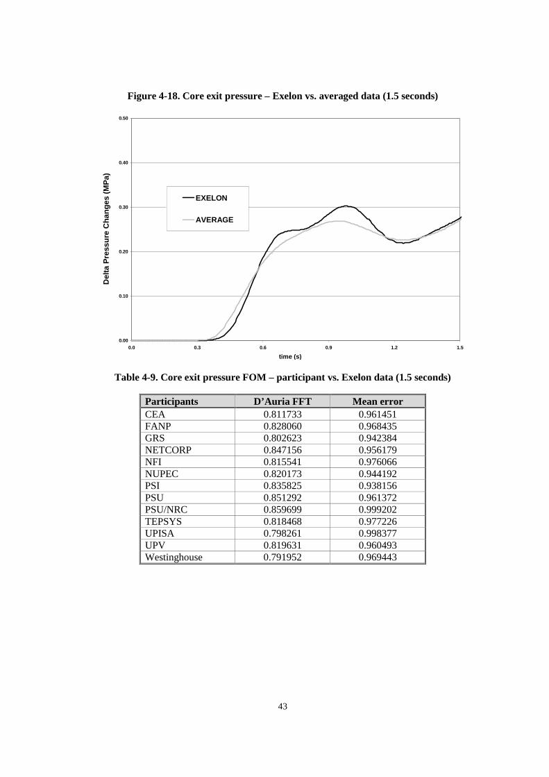
Figure 4-18. Core exit pressure – Exelon vs. averaged data (1.5 seconds) ................................ 43

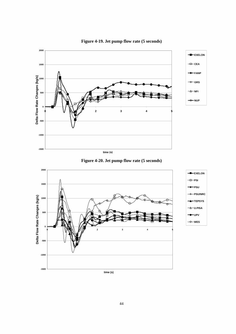
Figure 4-19. Jet pump flow rate (5 seconds) .............................................................................. 44

Figure 4-20. Jet pump flow rate (5 seconds) .............................................................................. 44

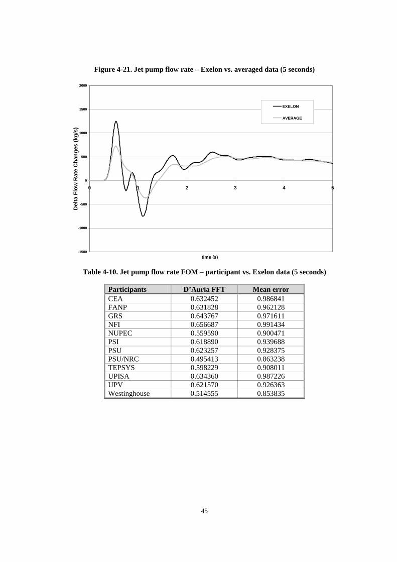
Figure 4-21. Jet pump flow rate – Exelon vs. averaged data (5 seconds) .................................. 45

Figure 4-22. Jet pump flow rate (1.5 seconds) ........................................................................... 46

Figure 4-23. Jet pump flow rate (1.5 seconds) ........................................................................... 46

8

Figure 4-24. Jet pump flow rate – Exelon vs. averaged data (5 seconds) .................................. 47

Figure 4-25. Core in-channel flow rate (5 seconds) ................................................................... 48

Figure 4-26. Core in-channel flow rate (5 seconds) ................................................................... 48

Figure 4-27. Core in-channel flow rate – Exelon vs. averaged data (5 seconds) ....................... 49

Figure 4-28. Core in-channel flow rate (1.5 seconds) ................................................................ 50

Figure 4-29. Core in-channel flow rate (1.5 seconds) ................................................................ 50

Figure 4-30. Core in-channel flow rate – Exelon vs. averaged data (1.5 seconds) .................... 51

Figure 4-31. Steam bypass flow rate (5 seconds.) ...................................................................... 52

Figure 4-32. Steam bypass flow rate (5 seconds)....................................................................... 52

Figure 4-33. Steam bypass flow rate – Exelon vs. averaged data (5 seconds) ........................... 53

Figure 4-34. Steam bypass flow rate (1.5 seconds).................................................................... 54

Figure 4-35. Steam bypass flow rate (1.5 seconds).................................................................... 54

Figure 4-36. Steam bypass flow rate – Exelon vs. averaged data (1.5 seconds) ........................ 55

Figure 4-37. Turbine inlet pressure (5 seconds) ......................................................................... 56

Figure 4-38. Turbine inlet pressure (5 seconds) ......................................................................... 56

Figure 4-39. Turbine inlet pressure (1.5 seconds) ...................................................................... 58

Figure 4-40. Turbine inlet pressure (1.5 seconds) ...................................................................... 58

Figure 4-41. RETRAN PB2 thermal-hydraulic model............................................................... 61

Figure A-1. TEPSYS modifications in control block INTM..................................................... 79

Figure B-1. CEA nodalisation diagram..................................................................................... 88

Figure B-2. FANP nodalisation diagram................................................................................... 91

Figure B-3. GRS reactor pressure vessel nodalisation schema ................................................. 94

Figure B-4. GRS steam line nodalisation schema..................................................................... 95

Figure B-5. NETCORP reactor vessel nodalisation.................................................................. 99

Figure B-6. NETCORP schematic of BWR NSSS representation............................................ 99

Figure B-7. NETCORP’s method of characteristics of main system........................................ 100

9

Figure B-8. NETCORP schematic of reactor vessel geometry for jet pumps........................... 101

Figure B-9. NETCORP flow diagram within reactor vessel for jet pumps .............................. 102

Figure B-10. NETCORP DNB/3D equations ............................................................................. 102

Figure B-11. NFI TRAC-BF1 nodalisation diagram .................................................................. 103

Figure B-12. NFI TRAC-BF1 steam line nodalisation ............................................................... 104

Figure B-13. NUPEC Peach Bottom 2 plant nodalisation .......................................................... 106

Figure B-14. PSI nodalisation of the reactor vessel .................................................................... 110

Figure B-15. PSI nodalisation of the channels............................................................................ 111

Figure B-16. PSI nodalisation of the steam line.......................................................................... 112

Figure B-17. Nodalisation of the steam separator region............................................................ 114

Figure B-18. PSU TRAC-BF1 nodalisation................................................................................ 116

Figure B-19. PSU/NRC TRAC-M nodalisation.......................................................................... 119

Figure B-20. PSU/NRC TRAC-M jet pump nodalisation........................................................... 120

Figure B-21. PSU/NRC TRAC-M separator nodalisation .......................................................... 120

Figure B-22. TEPSYS TRAC-BF1 plant model ......................................................................... 121

Figure B-23. UPISA RELAP5 model ......................................................................................... 124

Figure B-24. UPISA steam line simplified schema .................................................................... 124

Figure B-25. UPV thermal-hydraulic nodalisation ..................................................................... 127

Figure B-26. UPV thermal-hydraulic channel map .................................................................... 128

Figure B-27. UPV steam line nodalisation.................................................................................. 128

List of Tables

Table 1-1. List of participants in Exercise 1 of the BWR TT benchmark............................... 14

Table 2.3-1. PB2 TT2 initial conditions from process computer P1 edit................................... 16

Table 2.3-2. PB2 TT2 initial core average axial power distribution from P1 edit ..................... 17

Table 2.4-1. PB TT2 event timing (time in milliseconds).......................................................... 18

Table 4-1. Participant models used in Exercise 1 of the BWR TT benchmark....................... 29

10

Table 4-2. Core inlet enthalpy – deviation (ei) and FOM ....................................................... 30

Table 4-3. Core pressure drop – deviation (ei) and FOM........................................................ 31

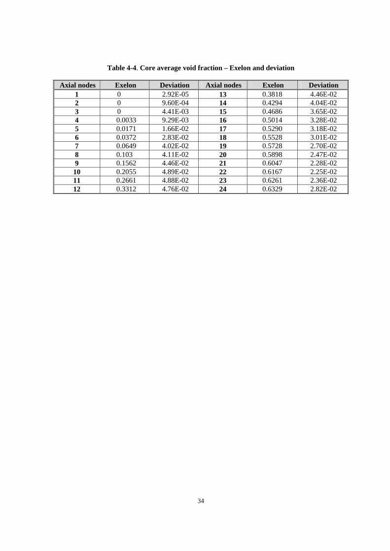
Table 4-4. Core average void fraction – Exelon and deviation............................................... 34

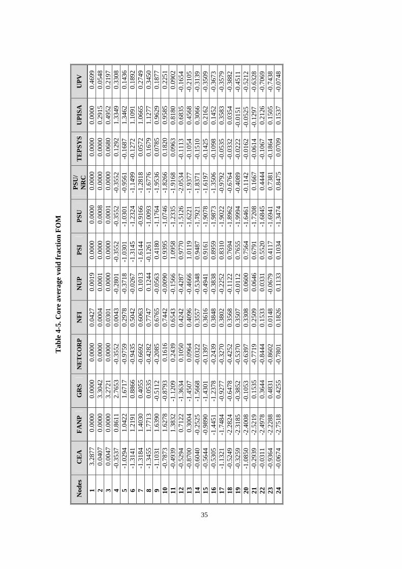
Table 4-5. Core average void fraction FOM........................................................................... 35

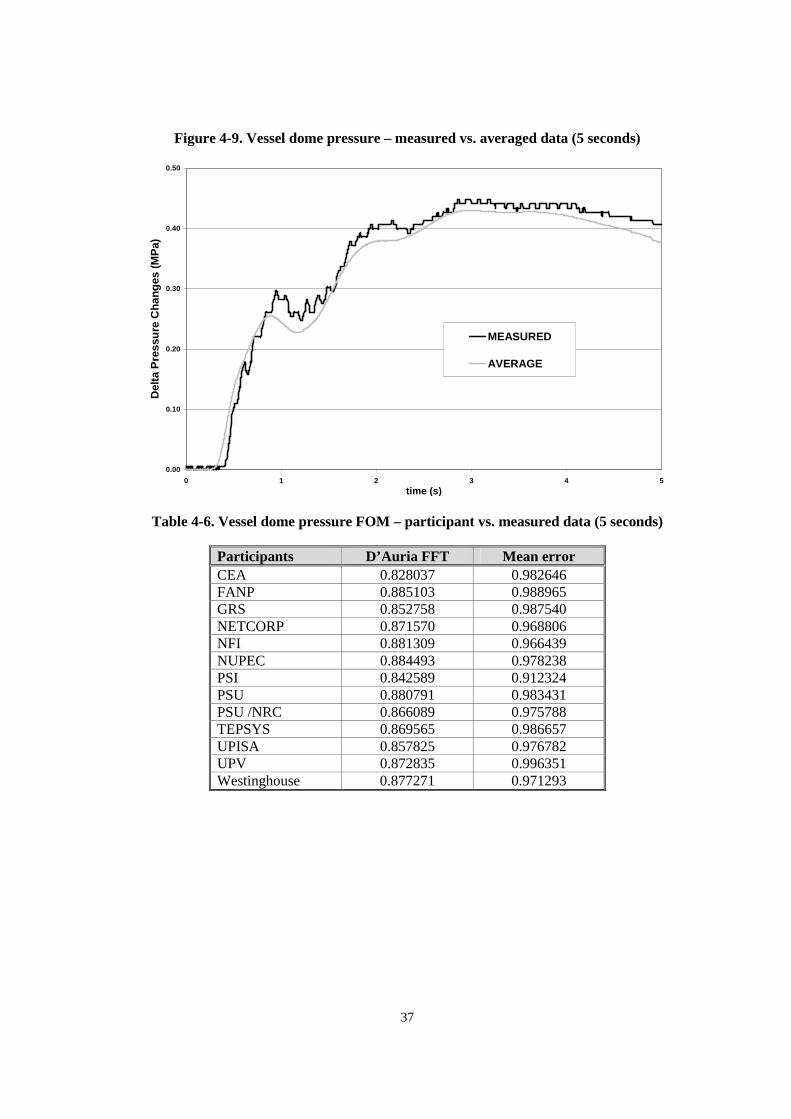
Table 4-6. Vessel dome pressure FOM – participant vs. measured data (5 seconds) ............. 37

Table 4-7. Vessel dome pressure FOM – participant vs. measured data (1.5 seconds) .......... 39

Table 4-8. Core exit pressure FOM – participant vs. Exelon data (5 seconds)....................... 41

Table 4-9. Core exit pressure FOM – participant vs. Exelon data (1.5 seconds).................... 43

Table 4-10. Jet pump flow rate FOM – participant vs. Exelon data (5 seconds) ...................... 45

Table 4-11. Jet pump flow rate FOM – participant vs. Exelon data (1.5 seconds) ................... 47

Table 4-12. Core in-channel flow rate FOM – participant vs. Exelon data (5 seconds) ........... 49

Table 4-13. Core in-channel flow rate FOM – participant vs. Exelon data (1.5 seconds) ........ 51

Table 4-14. Steam bypass flow rate FOM – participant vs. Exelon data (5 seconds)............... 53

Table 4-15. Steam bypass flow rate FOM – participant vs. Exelon data (1.5 seconds)............ 55

Table 4-16. Turbine inlet pressure FOM – participant vs. averaged data (5 seconds).............. 57

Table 4-17. Turbine inlet pressure FOM – participant vs. averaged data (1.5 seconds)........... 57

Table 4-18. Sequence of events ................................................................................................ 59

Table 4-19. Time of the maximum peak ................................................................................... 59

Table 4-20. Maximum peak value (delta changes) ................................................................... 60

Table A-1. TEPSYS reference numerical options in ENTRÉE and valve parameters ............ 79

Table B-1. UPISA steam line and bypass system geometrical data ........................................ 123

Table B-2. UPISA decay constant and fractions of delayed neutrons ..................................... 125

11

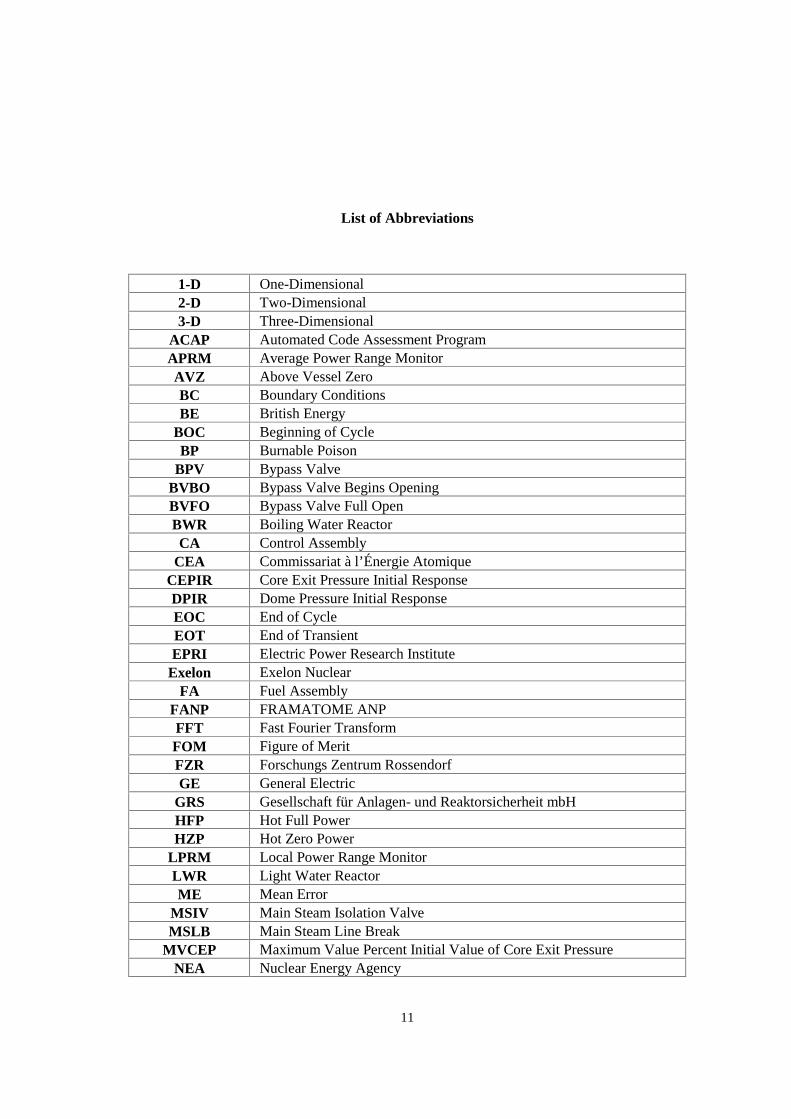
List of Abbreviations

1-D One-Dimensional 2-D Two-Dimensional 3-D Three-Dimensional

ACAP Automated Code Assessment Program APRM Average Power Range Monitor AVZ Above Vessel Zero BC Boundary Conditions BE British Energy

BOC Beginning of Cycle BP Burnable Poison

BPV Bypass Valve BVBO Bypass Valve Begins Opening BVFO Bypass Valve Full Open BWR Boiling Water Reactor CA Control Assembly

CEA Commissariat à l’Énergie Atomique CEPIR Core Exit Pressure Initial Response DPIR Dome Pressure Initial Response EOC End of Cycle EOT End of Transient EPRI Electric Power Research Institute

Exelon Exelon Nuclear FA Fuel Assembly

FANP FRAMATOME ANP FFT Fast Fourier Transform FOM Figure of Merit FZR Forschungs Zentrum Rossendorf GE General Electric

GRS Gesellschaft für Anlagen- und Reaktorsicherheit mbH HFP Hot Full Power HZP Hot Zero Power

LPRM Local Power Range Monitor LWR Light Water Reactor ME Mean Error

MSIV Main Steam Isolation Valve MSLB Main Steam Line Break

MVCEP Maximum Value Percent Initial Value of Core Exit Pressure NEA Nuclear Energy Agency

12

NEM Nodal Expansion Method NETCORP Nuclear Engineering Technology Corporation

NFI Nuclear Fuel Industries Ltd. NP Normalised Power

NPP Nuclear Power Plant NRC US Nuclear Regulatory Commission NRS Nuclear Reactor Systems NSC Nuclear Science Committee NSSS Nuclear Steam Supply System

NUPEC Nuclear Power Engineering Corporation OECD Organisation for Economic Co-operation and Development

PB Peach Bottom Atomic Power Station PB2 Peach Bottom Atomic Power Station Unit 2

PECo Philadelphia Electric Company PSI Paul Scherrer Institute PSU Pennsylvania State University PWR Pressurised Water Reactor SRV Safety Relief Valve

TEPSYS TEPCO Systems Corporation T-H Thermal-Hydraulic TSV Turbine Stop Valve

TSVC Turbine Stop Valve Closing TT Turbine Trip

TT2 Turbine Trip Test 2 UPISA University of Pisa UPV Universidad Politecnica de Valencia VBA Visual Basic for Applications WES Westinghouse Atom AB

13

Chapter 1

INTRODUCTION

Prediction of a nuclear power plant’s behaviour under both normal and abnormal conditions has important ramifications for safety and economic operations. Such prediction is only possible using highly sophisticated computer codes given the complexity of nuclear power plants. Incorporation of full three-dimensional (3-D) models of the reactor core into system transient codes allows for a “best-estimate” calculation of interactions between core behaviour and plant dynamics. Recent progress in computer technology has made the development of such coupled code systems (thermal-hydraulic and neutron kinetics) feasible. Considerable effort has been made by various countries and organisations in this direction. In order to verify the capability of the coupled codes for the analysis of complex transients with coupled core-plant interactions and to fully test thermal-hydraulic coupling, appropriate light water reactor (LWR) transient benchmarks need to be developed on a higher best-estimate level. Previous sets of transient benchmark problems separately addressed system transients (designed mainly for thermal-hydraulic system codes with point kinetics models) and core transients (designed for thermal-hydraulic core boundary condition models coupled with a 3-D neutron kinetics model). The Nuclear Energy Agency (NEA) of the Organisation for Economic Co-operation and Development (OECD) has recently completed, under the sponsorship of the US Nuclear Regulatory Commission (NRC), a PWR Main Steam Line Break (MSLB) benchmark [1] against coupled thermal-hydraulic and neutron kinetics codes.

A benchmark team from The Pennsylvania State University (PSU) was responsible for developing the benchmark specifications, assisting the participants and co-ordinating the benchmark activities. The benchmark was well-received by the international community. The participants of the PWR MSLB benchmark felt that there should be a similar benchmark against the codes for a BWR plant transient. A turbine trip (TT) transient in a BWR is a pressurisation event in which the coupling between core phenomena and system dynamics plays an important role. In addition, the available real plant experimental data [3-5] makes such a benchmark problem quite valuable. The NEA, OECD and US NRC have approved the BWR TT benchmark for the purpose of validating advanced-system best-estimate analysis codes.

As a result, a benchmark project has been established in order to test the coupled system (thermal-hydraulic/neutron kinetics) codes by modelling a PB2 (a GE-designed BWR/4) turbine trip transient with a sudden closure of the turbine stop valve. Three turbine trip transients at different power levels were performed at the Peach Bottom (PB2) BWR/4 nuclear power plant (NPP) prior to shutdown for refuelling at the end of Cycle 2 in April 1977. The second test was selected for the benchmark to investigate the effect of the pressurisation transient (following the sudden closure of the turbine stop valve) on the neutron flux in the reactor core. In a best-estimate manner the test conditions approached the design basis conditions as much as possible. The actual data were collected, including a compilation of reactor design and operating data for Cycles 1 and 2 of PB, as well as the plant transient experimental data. The transient was selected for this benchmark because it is a dynamically complex event for which neutron kinetics in the core were coupled with thermal-hydraulics in the reactor primary system.

14

The purposes of this benchmark are met through the application of three exercises, which are described in Volume 1 of the OECD/NRC BWR TT Benchmark – Final Specifications [2]. The purpose of the first exercise is to test the thermal-hydraulic system response and to initialise the participants’ system models. Core power response is provided to reproduce the actual test results, using either power or reactivity versus time data. The second exercise has two steady state conditions – hot zero power (HZP) conditions and initial conditions of TT2. The purpose of Exercise 2 is to provide a clean initialisation of the coupled core models since the core thermal-hydraulic boundary conditions are provided. The last exercise, Exercise 3, is the best estimate for coupled 3-D core/thermal-hydraulic system modelling. This exercise combines elements of the first two exercises of this benchmark and is an analysis of the transient in its entirety. Exercise 3 also includes extreme scenarios, which provide the opportunity to better test the code coupling and feedback modelling.

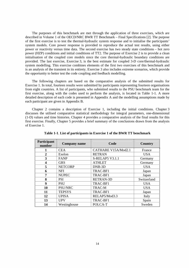
The following chapters are based on the comparative analysis of the submitted results for Exercise 1. In total, fourteen results were submitted by participants representing fourteen organisations from eight countries. A list of participants, who submitted results to the PSU benchmark team for the first exercise, along with the codes used to perform the analysis, is located in Table 1-1. A more detailed description of each code is presented in Appendix A and the modelling assumptions made by each participant are given in Appendix B.

Chapter 2 contains a description of Exercise 1, including the initial conditions. Chapter 3 discusses the utilised comparative statistical methodology for integral parameters, one-dimensional (1-D) values and time histories. Chapter 4 provides a comparative analysis of the final results for this first exercise. Finally, Chapter 5 provides a brief summary of the conclusions drawn from the analysis of Exercise 1.

Table 1-1. List of participants in Exercise 1 of the BWR TT benchmark

Participant number

Company name Code Country

1 CEA CATHARE V15A/Mod2.1 France 2 Exelon RETRAN USA 3 FANP S-RELAP5 V3.1.1 Germany 4 GRS ATHLET Germany 5 NETCORP DNB-3D USA 6 NFI TRAC-BF1 Japan 7 NUPEC TRAC-BF1 Japan 8 PSI RETRAN-3D Switzerland 9 PSU TRAC-BF1 USA

10 PSU/NRC TRAC-M USA 11 TEPSYS TRAC-BF1 Japan 12 UPISA RELAP5/Mod3.3 Italy 13 UPV TRAC-BF1 Spain 14 Westinghouse POLCA-T Sweden

15

Chapter 2

DESCRIPTION OF EXERCISE 1

2.1 General

The first exercise consists of performing a system thermal-hydraulic calculation (no neutron kinetics model involved; core power or reactivity as a function of time is provided as an input) for the PB2 TT transient. The purpose of the first exercise is to test the thermal-hydraulic system response and to initialise the participants’ system models. This approach is used to develop/refine key sub-models of steam lines, steam bypass systems, jet pumps, steam separators and the upper downcomer region where a distinct steam-water interface exists.

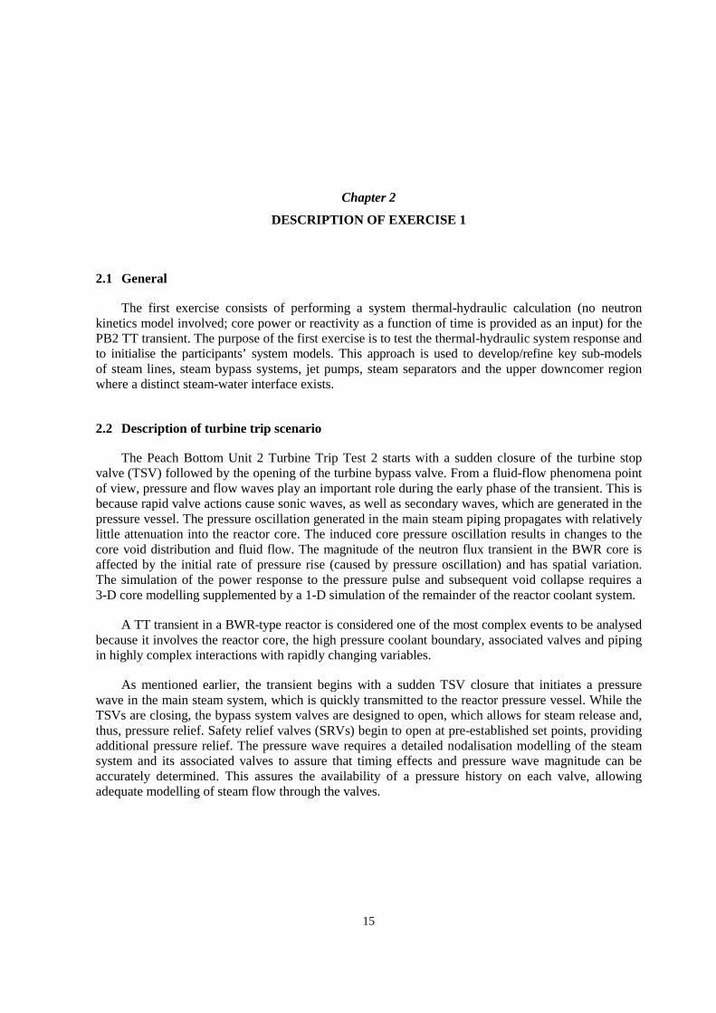
2.2 Description of turbine trip scenario

The Peach Bottom Unit 2 Turbine Trip Test 2 starts with a sudden closure of the turbine stop valve (TSV) followed by the opening of the turbine bypass valve. From a fluid-flow phenomena point of view, pressure and flow waves play an important role during the early phase of the transient. This is because rapid valve actions cause sonic waves, as well as secondary waves, which are generated in the pressure vessel. The pressure oscillation generated in the main steam piping propagates with relatively little attenuation into the reactor core. The induced core pressure oscillation results in changes to the core void distribution and fluid flow. The magnitude of the neutron flux transient in the BWR core is affected by the initial rate of pressure rise (caused by pressure oscillation) and has spatial variation. The simulation of the power response to the pressure pulse and subsequent void collapse requires a 3-D core modelling supplemented by a 1-D simulation of the remainder of the reactor coolant system.

A TT transient in a BWR-type reactor is considered one of the most complex events to be analysed because it involves the reactor core, the high pressure coolant boundary, associated valves and piping in highly complex interactions with rapidly changing variables.

As mentioned earlier, the transient begins with a sudden TSV closure that initiates a pressure wave in the main steam system, which is quickly transmitted to the reactor pressure vessel. While the TSVs are closing, the bypass system valves are designed to open, which allows for steam release and, thus, pressure relief. Safety relief valves (SRVs) begin to open at pre-established set points, providing additional pressure relief. The pressure wave requires a detailed nodalisation modelling of the steam system and its associated valves to assure that timing effects and pressure wave magnitude can be accurately determined. This assures the availability of a pressure history on each valve, allowing adequate modelling of steam flow through the valves.

16

2.3 Initial steady state conditions

The reference design for the BWR is derived from real reactor, plant and operation data for the PB2 NPP and it is based on the information provided in the EPRI reports [3-6] as well as some additional sources such as the PECo Energy Topical report [7].

Peach Bottom Atomic Power Station Unit 2 is a GE-designed BWR/4 with a rated thermal power of 3 293 MW, a rated core flow of 12 915 kg/s (102.5 × 106 lb/hr), a rated steam flow of 1 685 kg/s (13.37 × 106 lb/hr) and a turbine inlet pressure of 6.65 MPa (965 psia). The nuclear steam supply system (NSSS) has turbine-driven feed pumps and a two-loop M-G driven recirculation system, feeding a total of 20 jet pumps. In total, there are four steam lines and each has a flow-limiting nozzle, main steam isolation valves (MSIVs), safety relief valves and a turbine stop valve. The steam bypass system consists of nine bypass valves (BPVs) mounted on a common header, which is connected to each of the four steam lines.

There are 764 fuel bundles with an active fuel length of 365.76 cm (12 ft) in the core region. The fuel bundles consist of 576 original 7 × 7 fuel bundles with P/D (pitch/outer diameter) equal to 1.87452 cm/1.43002 cm (0.738 in/0.563 in) and 188 partially reloaded 8 × 8 fuel bundles with P/D equal to 1.62560 cm/1.25222 cm (0.640 in/0.493 in). Additionally, the core region includes 185 control rods (CRs). For the reactor protection system (RPS), control systems for reactor pressure, recirculation flow, feedwater flow and reactor water level are commonly used in reactors of this design.

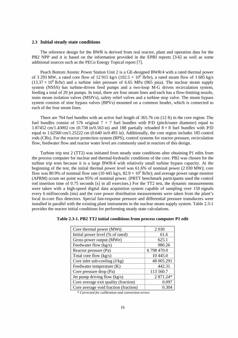
Turbine trip test 2 (TT2) was initiated from steady state conditions after obtaining P1 edits from the process computer for nuclear and thermal-hydraulic conditions of the core. PB2 was chosen for the turbine trip tests because it is a large BWR/4 with relatively small turbine bypass capacity. At the beginning of the test, the initial thermal power level was 61.6% of nominal power (2 030 MW); core flow was 80.9% of nominal flow rate (10 445 kg/s, 82.9 × 106 lb/hr); and average power range monitor (APRM) scram set point was 95% of nominal power. (PBTT benchmark participants used the control rod insertion time of 0.75 seconds [s] in all exercises.) For the TT2 test, the dynamic measurements were taken with a high-speed digital data acquisition system capable of sampling over 150 signals every 6 milliseconds (ms) and the core power distribution measurements were taken from the plant’s local in-core flux detectors. Special fast-response pressure and differential pressure transducers were installed in parallel with the existing plant instruments in the nuclear steam supply system. Table 2.3-1 provides the reactor initial conditions for performing steady state calculations.

Table 2.3-1. PB2 TT2 initial conditions from process computer P1 edit

Core thermal power (MWt) 2 030.000 Initial power level (% of rated) 61.600 Gross power output (MWe) 625.100 Feedwater flow (kg/s) 980.260 Reactor pressure (Pa) 6 798 470.000 Total core flow (kg/s) 10 445.000 Core inlet sub-cooling (J/kg) 48 005.291 Feedwater temperature (K) 442.310 Core pressure drop (Pa) 113 560.700 Jet pump driving flow (kg/s) 2 871.24* Core average exit quality (fraction) 0.097 Core average void fraction (fraction) 0.304

* Corrected for calibration and conversion errors

17

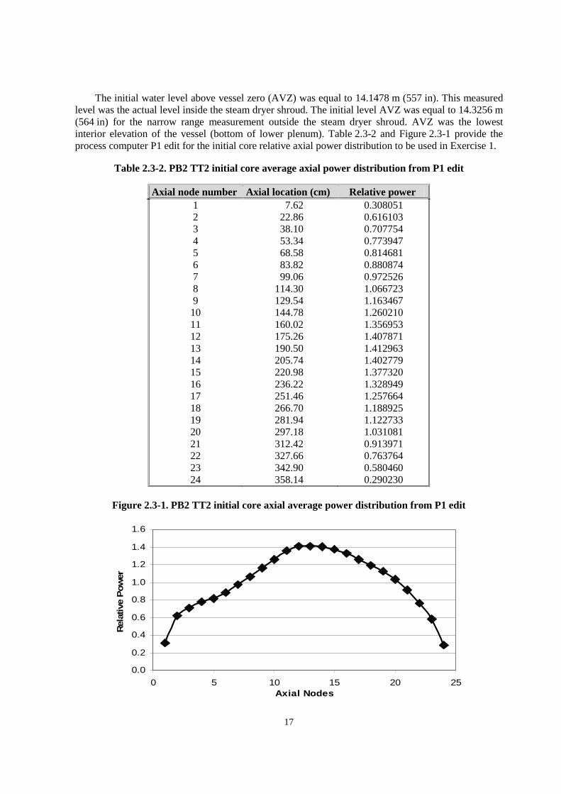
The initial water level above vessel zero (AVZ) was equal to 14.1478 m (557 in). This measured level was the actual level inside the steam dryer shroud. The initial level AVZ was equal to 14.3256 m (564 in) for the narrow range measurement outside the steam dryer shroud. AVZ was the lowest interior elevation of the vessel (bottom of lower plenum). Table 2.3-2 and Figure 2.3-1 provide the process computer P1 edit for the initial core relative axial power distribution to be used in Exercise 1.

Table 2.3-2. PB2 TT2 initial core average axial power distribution from P1 edit

Axial node number Axial location (cm) Relative power 1 2 3 4 5 6 7 8 9 10 11 12 13 14 15 16 17 18 19 20 21 22 23 24

017.62 122.86 138.10 153.34 168.58 183.82 199.06 114.30 129.54 144.78 160.02 175.26 190.50 205.74 220.98 236.22 251.46 266.70 281.94 297.18 312.42 327.66 342.90 358.14

0.308051 0.616103 0.707754 0.773947 0.814681 0.880874 0.972526 1.066723 1.163467 1.260210 1.356953 1.407871 1.412963 1.402779 1.377320 1.328949 1.257664 1.188925 1.122733 1.031081 0.913971 0.763764 0.580460 0.290230

Figure 2.3-1. PB2 TT2 initial core axial average power distribution from P1 edit

0.0

0.2

0.4

0.6

0.8

1.0

1.2

1.4

1.6

0 5 10 15 20 25Axial Nodes

Rel

ativ

e P

ow

er

18

2.4 Transient calculations

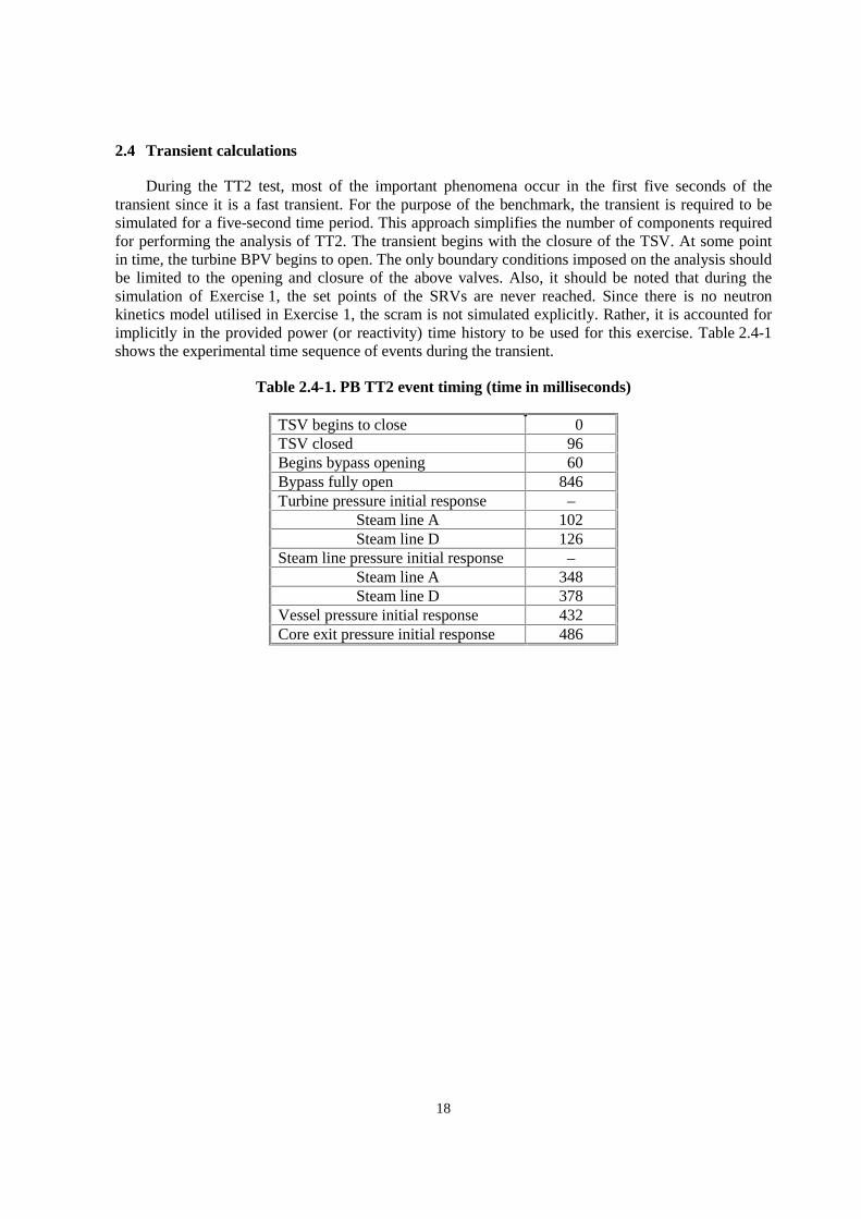
During the TT2 test, most of the important phenomena occur in the first five seconds of the transient since it is a fast transient. For the purpose of the benchmark, the transient is required to be simulated for a five-second time period. This approach simplifies the number of components required for performing the analysis of TT2. The transient begins with the closure of the TSV. At some point in time, the turbine BPV begins to open. The only boundary conditions imposed on the analysis should be limited to the opening and closure of the above valves. Also, it should be noted that during the simulation of Exercise 1, the set points of the SRVs are never reached. Since there is no neutron kinetics model utilised in Exercise 1, the scram is not simulated explicitly. Rather, it is accounted for implicitly in the provided power (or reactivity) time history to be used for this exercise. Table 2.4-1 shows the experimental time sequence of events during the transient.

Table 2.4-1. PB TT2 event timing (time in milliseconds)

TSV begins to close 110 TSV closed 096 Begins bypass opening 160 Bypass fully open 846 Turbine pressure initial response –

Steam line A 102 Steam line D 126

Steam line pressure initial response – Steam line A 348 Steam line D 378

Vessel pressure initial response 432 Core exit pressure initial response 486

19

Chapter 3

METHODOLOGIES FOR COMPARATIVE ANALYSIS

As mentioned in Chapter 1, each of the 14 participants submitted various data that were available for statistical analysis. The submitted results were categorised by nature of the data. For Exercise 1, the categories were: integral parameter values, 1-D distributions and time histories.

In addition, the submitted data could be distinguished according to the reference data used in the comparative analysis. The reference data used in the Exercise 1 comparative analysis were called: measured data, Exelon data and averaged data.

Measured data is the set of original recorded data during the second turbine trip transient test. In the case of unavailable measured data, Exelon results (so-called Exelon data) were used as reference results for the comparison. The main reason for this approach is that the Exelon results were already extensively validated with the measured data. In other words, the Exelon data agree quite well with the measured data and this agreement was published in the PECo Topical Report, which was submitted to US NRC [7]. It should be noted that the current operator of PB2 NPP is Exelon Nuclear. The former operator, the Philadelphia Electric Company (PECo), recently merged with Exelon Nuclear. In the event of a lack of measured data and/or Exelon data for a given parameter, the reference solution for each requested parameter is based on the statistical mean value (so-called averaged data) of all submitted results.

3.1 Standard techniques for the comparison of results

In Exercise 1 of this benchmark, several types of data were analysed and the results of all participants were compared. The data types were:

� Integral parameter values.

� One-dimensional (1-D) axial distributions.

� Time histories.

It was necessary to develop a suite of statistical methods for each of these data types, which were applied in the comparative analysis. What follows is a description of each of these methods.

3.1.1 Integral parameter values

These parameters include such values as core inlet enthalpy and core average pressure drop for initial steady state conditions. Since measured data exist for both core inlet enthalpy and core average pressure drop, standard deviation and figure of merit (FOM) are calculated in Eqs. (3.1-3.3).

20

� �1

2

�

��

N

xx Measuredi

(3.1)

where � is the standard deviation, xi is the data submitted by each participant and N is the total number of received results.

The FOM is computed as follows:

i = ei/� (3.2)

ei = xi – xMeasured (3.3)

where ei is the deviation for each participant result.

3.1.2 One-dimensional (1-D) axial distributions

Exercise 1 compared only one 1-D axial distribution, which was the core average axial void fraction distribution. The core average axial void fraction distribution is a function of height or number of axial nodes, and it can be displayed as an x-y plot. Similar methods of statistical analysis described in the previous section could be applied for each axial cell, the only difference being the reference data. In this case and in the event of a lack of measured data, the Exelon data were taken as reference for the comparison. Analyses were performed for each 1-D cell according to Eqs. (3.4-3.6):

� �1

2

�

��

N

xx Exeloni

(3.4)

where xi is each participant’s data and N is the total number of received results. FOM is computed as:

i = ei/� (3.5)

ei = xi – xExelon (3.6)

For each participant, a table was prepared that shows the deviations from mean and FOM at each axial position.

3.1.3 Time histories

Six different sets of time histories were submitted by the participants for Exercise 1. The submitted time histories included: dome pressure, core exit pressure, jet pump flow rate, core in-channel flow rate, steam bypass flow rate and turbine inlet pressure. The reference data for dome pressure comparison was the measured data. Since Exelon data were available for core exit pressure, jet pump flow rate, core in-channel flow rate and steam bypass flow rate, the comparisons were based on the Exelon data. It should be noted that for some of these categories there were measured data. However, the quality of this data (oscillating time histories) was not appropriate and the oscillatory behaviour of the data needed to be smoothed. The Exelon results show perfect agreement with the smoothed measured data. Due to the lack of measured and Exelon data, the statistical mean value of the submitted turbine pressure results (also called averaged data) was used as reference. The averaged data were calculated according to the equation that follows.

21

N

x

x

N

ii�

�

(3.7)

where xi is each participant’s value for specified time interval and N is total number of received results.

3.2 ACAP analysis

The comparative analysis was performed for code-to-data and code-to-code comparisons using the standard statistical methodology with the Automated Code Assessment Program (ACAP) [8]. ACAP is a tool developed to provide quantitative comparisons between nuclear reactor system code results and experimental measurements. This software was developed under a contract with PSU and the NRC for use in PSU’s code consolidation efforts. ACAP’s capabilities are described as follows:

� Draws upon a mathematical toolkit to compare experimental data and NRS code simulations.

� Returns quantitative FOMs associated with individual and suite comparisons.

� Accommodates the multiple data types encountered in NRS environments.

� Incorporates experimental uncertainty in the assessment.

� Provides “event windowing” capability.

� Accommodates inconsistencies between measured and computed independent variables (e.g. different time steps).

� Provides a framework for automated, tuneable weighting of component measures in the construction of overall FOM accuracy.

ACAP is a PC and UNIX station-based application that can be run interactively on PCs with Windows 95/98/NT, in batch mode on PCs as a Windows console application, or in batch mode on UNIX stations as a command line executable.

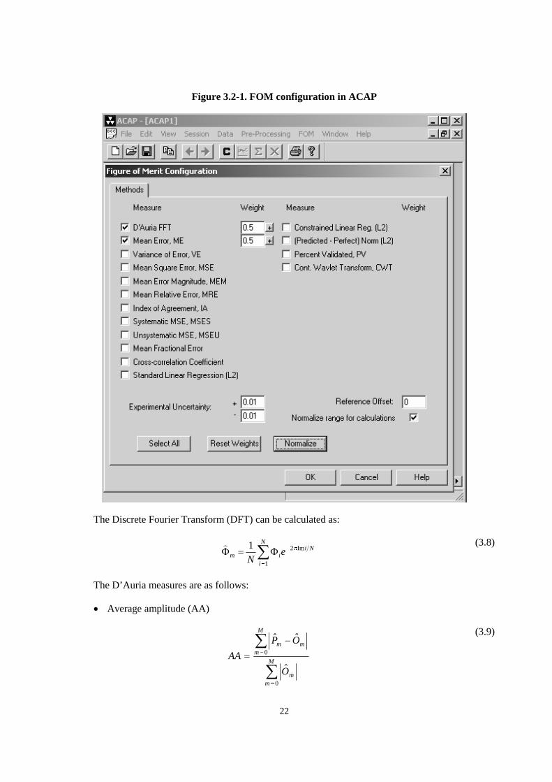
The D’Auria Fast Fourier Transformation (FFT) and Mean Error (ME) methods were used in FOM calculations for time histories [8,11]. Figure 3.2-1 shows a snapshot of the FOM configuration for ACAP calculations in Exercise 1 of the benchmark. These methods are advanced techniques for analysis of time history data. Eqs. (3.8-3.13) represent the theory portion of the D’Auria FFT and ME methods.

22

Figure 3.2-1. FOM configuration in ACAP

The Discrete Fourier Transform (DFT) can be calculated as:

��

��N

i

Niim e

N 1

Im21�

(3.8)

The D’Auria measures are as follows:

� Average amplitude (AA)

�

�

�

�

��

M

mm

M

mmm

O

OP

AA

0

0

(3.9)

23

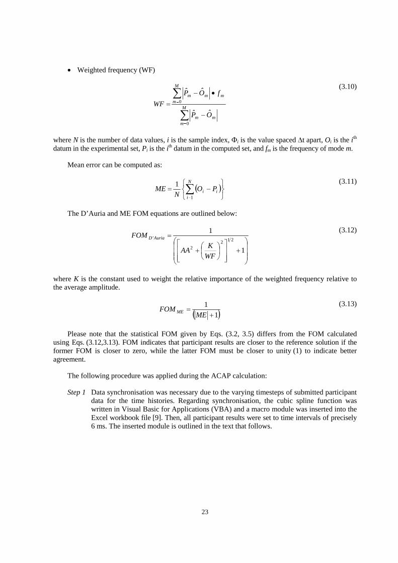
� Weighted frequency (WF)

�

�

�

�

�

��

M

mmm

m

M

mmm

OP

fOP

WF

0

0

(3.10)

where N is the number of data values, i is the sample index, i is the value spaced t apart, Oi is the ith datum in the experimental set, Pi is the ith datum in the computed set, and fm is the frequency of mode m.

Mean error can be computed as:

� ��

��

��

N

iii PO

NME

1

1

(3.11)

The D’Auria and ME FOM equations are outlined below:

��

�

�

��

�

��

��

�

��

��

��

�

1

1212

2

WF

KAA

FOM Auria’D (3.12)

where K is the constant used to weight the relative importance of the weighted frequency relative to the average amplitude.

� �1

1

��

MEFOM ME

(3.13)

Please note that the statistical FOM given by Eqs. (3.2, 3.5) differs from the FOM calculated using Eqs. (3.12,3.13). FOM indicates that participant results are closer to the reference solution if the former FOM is closer to zero, while the latter FOM must be closer to unity (1) to indicate better agreement.

The following procedure was applied during the ACAP calculation:

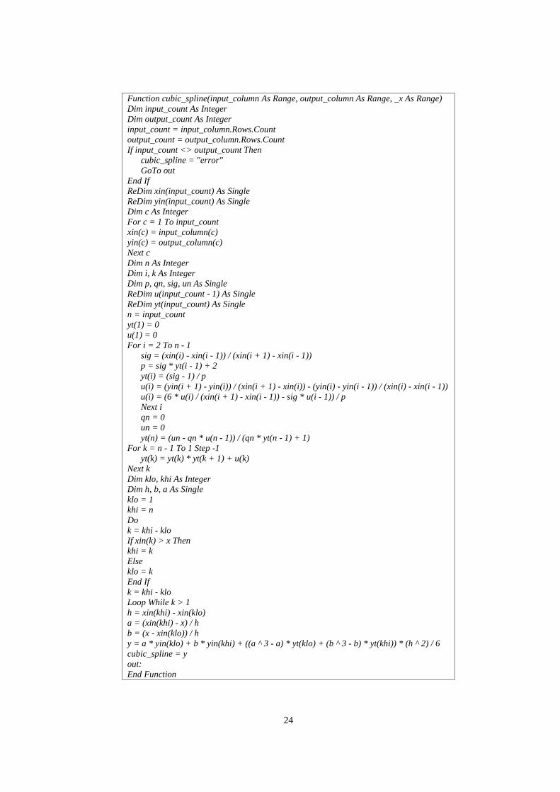
Step 1 Data synchronisation was necessary due to the varying timesteps of submitted participant data for the time histories. Regarding synchronisation, the cubic spline function was written in Visual Basic for Applications (VBA) and a macro module was inserted into the Excel workbook file [9]. Then, all participant results were set to time intervals of precisely 6 ms. The inserted module is outlined in the text that follows.

24

Function cubic_spline(input_column As Range, output_column As Range, _x As Range) Dim input_count As Integer Dim output_count As Integer input_count = input_column.Rows.Count output_count = output_column.Rows.Count If input_count <> output_count Then 000cubic_spline = "error" 000GoTo out End If ReDim xin(input_count) As Single ReDim yin(input_count) As Single Dim c As Integer For c = 1 To input_count xin(c) = input_column(c) yin(c) = output_column(c) Next c Dim n As Integer Dim i, k As Integer Dim p, qn, sig, un As Single ReDim u(input_count - 1) As Single ReDim yt(input_count) As Single n = input_count yt(1) = 0 u(1) = 0 For i = 2 To n - 1 000sig = (xin(i) - xin(i - 1)) / (xin(i + 1) - xin(i - 1)) 000p = sig * yt(i - 1) + 2 000yt(i) = (sig - 1) / p 000u(i) = (yin(i + 1) - yin(i)) / (xin(i + 1) - xin(i)) - (yin(i) - yin(i - 1)) / (xin(i) - xin(i - 1)) 000u(i) = (6 * u(i) / (xin(i + 1) - xin(i - 1)) - sig * u(i - 1)) / p 000Next i 000qn = 0 000un = 0 000yt(n) = (un - qn * u(n - 1)) / (qn * yt(n - 1) + 1) For k = n - 1 To 1 Step -1 000yt(k) = yt(k) * yt(k + 1) + u(k) Next k Dim klo, khi As Integer Dim h, b, a As Single klo = 1 khi = n Do k = khi - klo If xin(k) > x Then khi = k Else klo = k End If k = khi - klo Loop While k > 1 h = xin(khi) - xin(klo) a = (xin(khi) - x) / h b = (x - xin(klo)) / h y = a * yin(klo) + b * yin(khi) + ((a ^ 3 - a) * yt(klo) + (b ^ 3 - b) * yt(khi)) * (h ^ 2) / 6 cubic_spline = y out: End Function

25

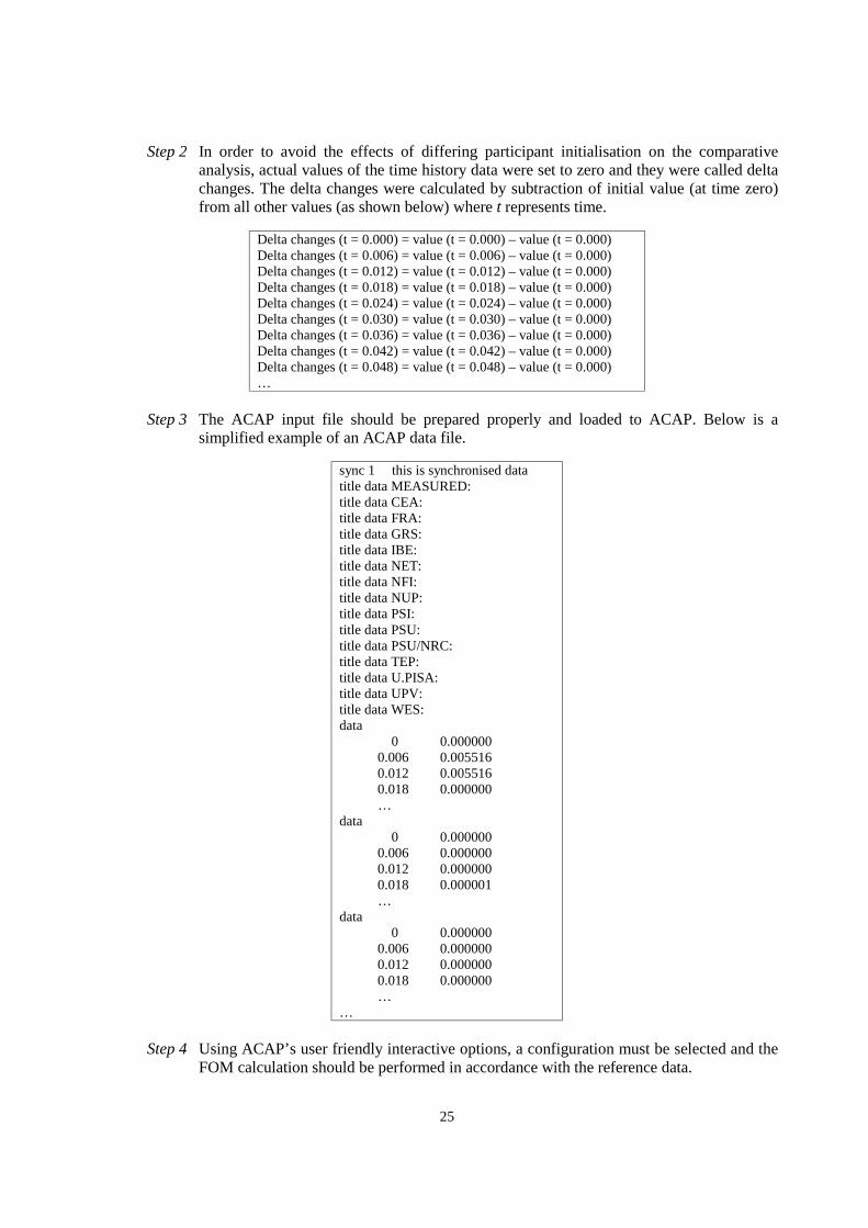
Step 2 In order to avoid the effects of differing participant initialisation on the comparative analysis, actual values of the time history data were set to zero and they were called delta changes. The delta changes were calculated by subtraction of initial value (at time zero) from all other values (as shown below) where t represents time.

Delta changes (t = 0.000) = value (t = 0.000) – value (t = 0.000) Delta changes (t = 0.006) = value (t = 0.006) – value (t = 0.000) Delta changes (t = 0.012) = value (t = 0.012) – value (t = 0.000) Delta changes (t = 0.018) = value (t = 0.018) – value (t = 0.000) Delta changes (t = 0.024) = value (t = 0.024) – value (t = 0.000) Delta changes (t = 0.030) = value (t = 0.030) – value (t = 0.000) Delta changes (t = 0.036) = value (t = 0.036) – value (t = 0.000) Delta changes (t = 0.042) = value (t = 0.042) – value (t = 0.000) Delta changes (t = 0.048) = value (t = 0.048) – value (t = 0.000) …

Step 3 The ACAP input file should be prepared properly and loaded to ACAP. Below is a

simplified example of an ACAP data file.

sync 1 this is synchronised data title data MEASURED: title data CEA: title data FRA: title data GRS: title data IBE: title data NET: title data NFI: title data NUP: title data PSI: title data PSU: title data PSU/NRC: title data TEP: title data U.PISA: title data UPV: title data WES: data 0 0.000000 0.006 0.005516 0.012 0.005516 0.018 0.000000 … data 0 0.000000 0.006 0.000000 0.012 0.000000 0.018 0.000001 … data 0 0.000000 0.006 0.000000 0.012 0.000000 0.018 0.000000 … …

Step 4 Using ACAP’s user friendly interactive options, a configuration must be selected and the

FOM calculation should be performed in accordance with the reference data.

27

Chapter 4

RESULTS AND DISCUSSION OF EXERCISE 1

The tables and figures in this chapter provide a comparison of participant results with the referencesolution for the parameters that have the greatest effect on the initial steady state and transient scenario.The tables show values of standard deviation and figure of merit (as defined in Chapter 3) for eachparticipant result and for a given parameter. This chapter contains figures that show the scatter of dataaround the reference solution.

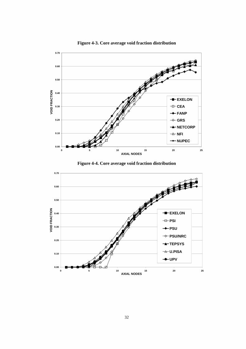
Participant models used in Exercise 1 are presented in Table 4-1. This table is categorised byusage of bypass model, decay heat and power model as well as by the number of core channels in theparticipant system models. Core inlet enthalpy, core average pressure drop and core averaged axialvoid fraction distribution are the selected parameters for steady state comparisons in this exercise. Forthese parameters, Figures 4-1 through 4-6 graphically illustrate the agreement or disagreement ofparticipant predictions. Tables 4-2 through 4-5 show values, deviations and figures of merit for eachparticipant result and given parameter.

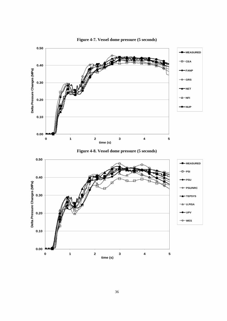
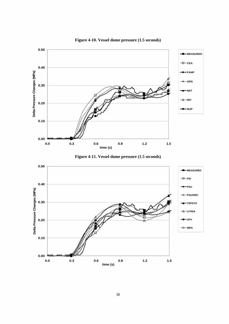
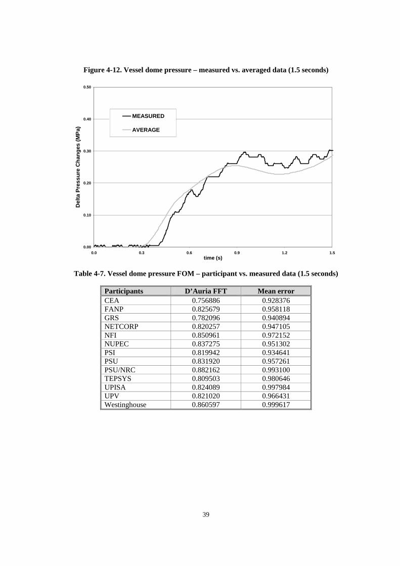
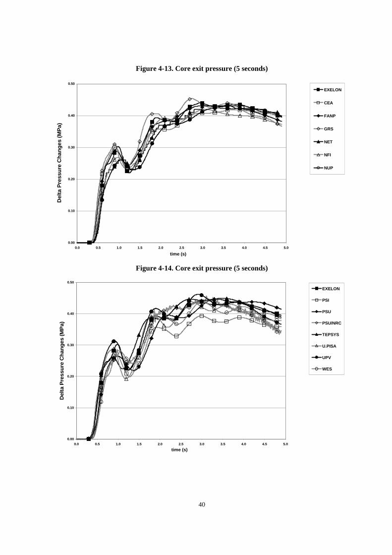
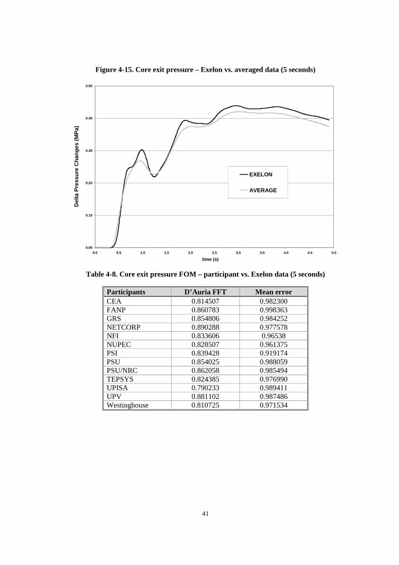
In the transient analysis, reactor vessel dome pressure, core exit pressure, jet pump flow rate (totalcore flow rate), core in-channel flow rate, steam bypass flow rate (turbine bypass flow rate) and turbineinlet pressure are the selected time histories for Exercise 1 comparisons. Time histories were analysedfor two different time intervals, which were 5 seconds and 1.5 seconds. Since this transient is a very fastone, the study focused on the initial 1.5 s period after performing the analysis on the 5 s period.Figures 4-7 through 4-40 compare the participant results with the reference solutions for each parameter.Reference solutions are also compared with the averaged values of participant results. In addition,Tables 4-6 through 4-17 show the ACAP FOM results for each parameter.

Although each of the 5 s time histories consisted of 833 data points and each of the 1.5 s timehistories consisted of 250 data points, few of these data points were marked in the figures. One markerfor each 50 points (for each 0.3 s time interval) was shown on the figures in order to make the figureslegible. For this purpose, a macro module was written in VBA for the Excel workbooks.

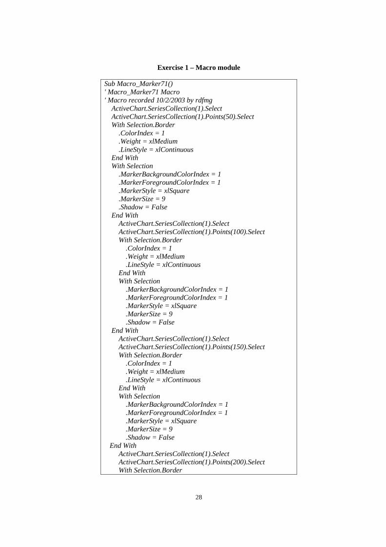
Participant marker types, marker frequencies and the thickness/colour of lines were unique andconsistent for all time history figures. For instance, the reference data (measured, Exelon or averaged)were always illustrated with the marker . Part of the macro module is subsequently shown.

28

Exercise 1 – Macro module

Sub Macro_Marker71()' Macro_Marker71 Macro' Macro recorded 10/2/2003 by rdfmg

ActiveChart.SeriesCollection(1).SelectActiveChart.SeriesCollection(1).Points(50).SelectWith Selection.Border

.ColorIndex = 1

.Weight = xlMedium

.LineStyle = xlContinuousEnd WithWith Selection

.MarkerBackgroundColorIndex = 1

.MarkerForegroundColorIndex = 1

.MarkerStyle = xlSquare

.MarkerSize = 9

.Shadow = FalseEnd With


.ColorIndex = 1

.Weight = xlMedium





.MarkerSize = 9



.ColorIndex = 1

.Weight = xlMedium





.MarkerSize = 9



29

Exercise 1 – Macro module continued

.ColorIndex = 1

.Weight = xlMedium





.MarkerSize = 9

.Shadow = False***continues for all desired data points and for all other figuresillustrated on the Excel chart***

End WithEnd Sub

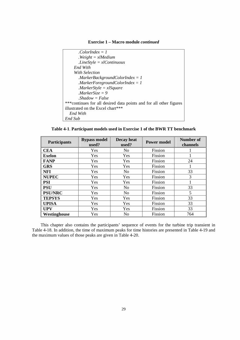
Table 4-1. Participant models used in Exercise 1 of the BWR TT benchmark

Participants Bypass modelused?

Decay heatused?

Power model Number ofchannels

CEA Yes No Fission 1Exelon Yes Yes Fission 1FANP Yes Yes Fission 24GRS Yes Yes Fission 1NFI Yes No Fission 33NUPEC Yes Yes Fission 3PSI Yes Yes Fission 1PSU Yes No Fission 33PSU/NRC Yes No Fission 5TEPSYS Yes Yes Fission 33UPISA Yes Yes Fission 33UPV Yes Yes Fission 33Westinghouse Yes No Fission 764

This chapter also contains the participants’ sequence of events for the turbine trip transient inTable 4-18. In addition, the time of maximum peaks for time histories are presented in Table 4-19 andthe maximum values of those peaks are given in Table 4-20.

30

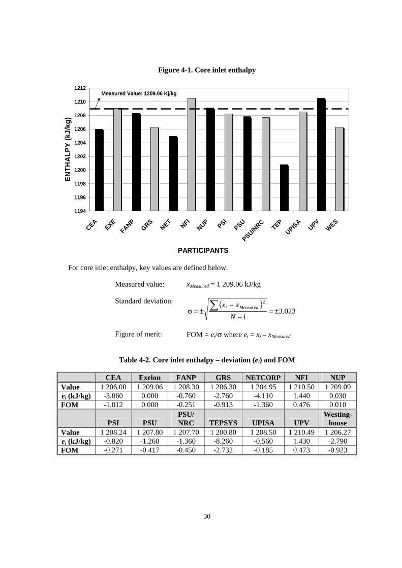
Figure 4-1. Core inlet enthalpy

Measured Value: 1209.06 Kj/kg

1194

1196

1198

1200

1202

1204

1206

1208

1210

1212

CEAEXE

FANPGRS

NETNFI

NUPPSI

PSU

PSU/NRC

TEP

UPISA

UPVW

ES

PARTICIPANTS

EN

TH

AL

PY

(kJ/

kg)

For core inlet enthalpy, key values are defined below.

Measured value: xMeasured = 1 209.06 kJ/kg

Standard deviation: ( )0233

1

2

.N

xx Measuredi ±=−

−±=σ �

Figure of merit: FOM = ei/σ where ei = xi – xMeasured

Table 4-2. Core inlet enthalpy – deviation (ei) and FOM

CEA Exelon FANP GRS NETCORP NFI NUPValue 1 206.00 1 209.06 1 208.30 1 206.30 1 204.95 1 210.50 1 209.09ei (kJ/kg) -3.060 0.000 -0.760 -2.760 -4.110 1.440 0.030FOM -1.012 0.000 -0.251 -0.913 -1.360 0.476 0.010

PSI PSUPSU/NRC TEPSYS UPISA UPV

Westing-house

Value 1 208.24 1 207.80 1 207.70 1 200.80 1 208.50 1 210.49 1 206.27ei (kJ/kg) -0.820 -1.260 -1.360 -8.260 -0.560 1.430 -2.790FOM -0.271 -0.417 -0.450 -2.732 -0.185 0.473 -0.923

31

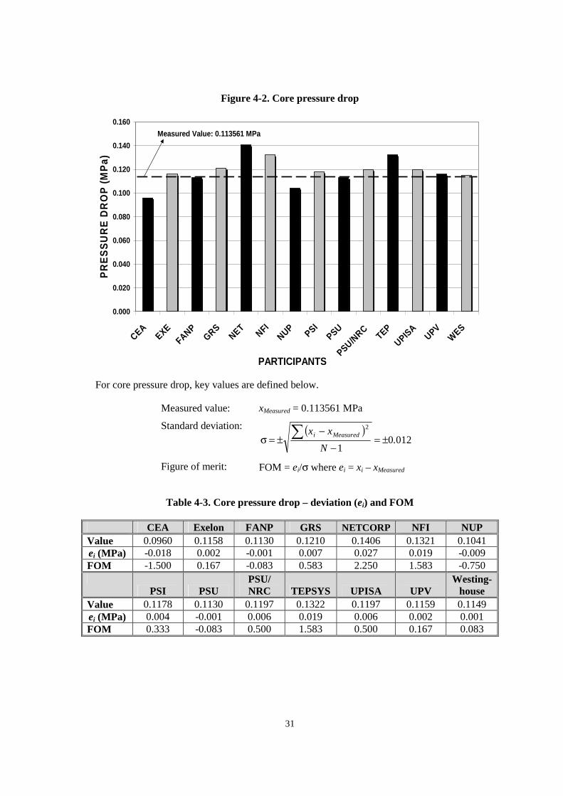
Figure 4-2. Core pressure drop

Measured Value: 0.113561 MPa

0.000

0.020

0.040

0.060

0.080

0.100

0.120

0.140

0.160

CEAEXE

FANPGRS

NETNFI

NUPPSI

PSU

PSU/NRC

TEP

UPISA

UPVW

ES

PARTICIPANTS

PR

ES

SU

RE

DR

OP

(MP

a)

For core pressure drop, key values are defined below.

Measured value: xMeasured = 0.113561 MPa

Standard deviation: ( )0120

1

2

.N

xx Measuredi ±=−

−±=σ �

Figure of merit: FOM = ei/σ where ei = xi – xMeasured

Table 4-3. Core pressure drop – deviation (ei) and FOM

CEA Exelon FANP GRS NETCORP NFI NUPValue 0.0960 0.1158 0.1130 0.1210 0.1406 0.1321 0.1041ei (MPa) -0.018 0.002 -0.001 0.007 0.027 0.019 -0.009FOM -1.500 0.167 -0.083 0.583 2.250 1.583 -0.750

PSI PSUPSU/NRC TEPSYS UPISA UPV

Westing-house

Value 0.1178 0.1130 0.1197 0.1322 0.1197 0.1159 0.1149ei (MPa) 0.004 -0.001 0.006 0.019 0.006 0.002 0.001FOM 0.333 -0.083 0.500 1.583 0.500 0.167 0.083

32

Figure 4-3. Core average void fraction distribution

0.00

0.10

0.20

0.30

0.40

0.50

0.60

0.70

0 5 10 15 20 25

AXIAL NODES

VO

IDF

RA

CT

ION

EXELON

CEA

FANP

GRS

NETCORP

NFI

NUPEC

Figure 4-4. Core average void fraction distribution

0.00

0.10

0.20

0.30

0.40

0.50

0.60

0.70

0 5 10 15 20 25AXIAL NODES

VO

IDF

RA

CT

ION

EXELON

PSI

PSU

PSU/NRC

TEPSYS

U.PISA

UPV

33

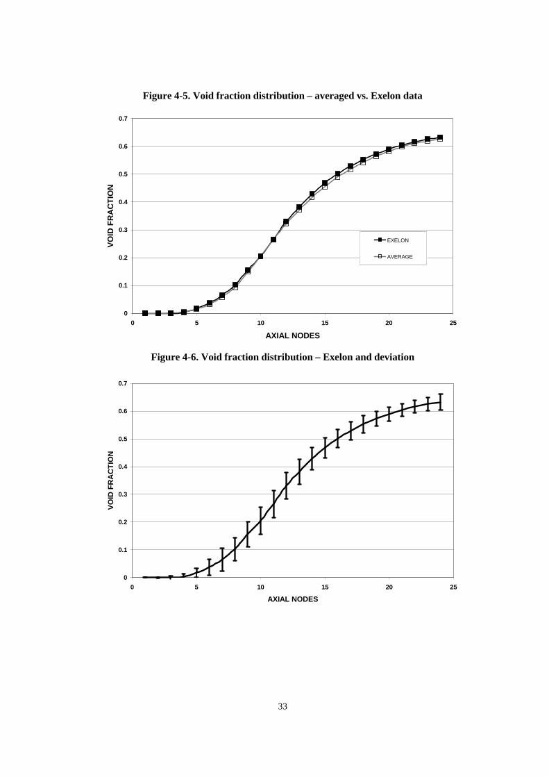
Figure 4-5. Void fraction distribution – averaged vs. Exelon data

0

0.1

0.2

0.3

0.4

0.5

0.6

0.7

0 5 10 15 20 25

AXIAL NODES

VO

IDF

RA

CT

ION

EXELON

AVERAGE

Figure 4-6. Void fraction distribution – Exelon and deviation

0

0.1

0.2

0.3

0.4

0.5

0.6

0.7

0 5 10 15 20 25

AXIAL NODES

VO

IDF

RA

CT

ION

34

Table 4-4. Core average void fraction – Exelon and deviation

Axial nodes Exelon Deviation Axial nodes Exelon Deviation1 00000 2.92E-05 13 0.3818 4.46E-022 00000 9.60E-04 14 0.4294 4.04E-023 00000 4.41E-03 15 0.4686 3.65E-024 0.0033 9.29E-03 16 0.5014 3.28E-025 0.0171 1.66E-02 17 0.5290 3.18E-026 0.0372 2.83E-02 18 0.5528 3.01E-027 0.0649 4.02E-02 19 0.5728 2.70E-028 0.1030 4.11E-02 20 0.5898 2.47E-029 0.1562 4.46E-02 21 0.6047 2.28E-0210 0.2055 4.89E-02 22 0.6167 2.25E-0211 0.2661 4.88E-02 23 0.6261 2.36E-0212 0.3312 4.76E-02 24 0.6329 2.82E-02

Tab

le4-

5.C

ore

aver

age

void

frac

tion

FO

M

Nod

esC

EA

FA

NP

GR

SN

ET

CO

RP

NF

IN

UP

PSI

PSU

PSU

/N

RC

TE

PSY

SU

PIS

AU

PV

103

.287

700

.000

000

.000

000

.000

00.

0427

00.0

019

0.00

0010

.000

010

.000

010

.000

00.

0000

10.4

699

200

.040

700

.000

003

.304

200

.000

00.

0004

00.0

001

0.00

0010

.000

810

.000

010

.000

00.

2915

10.0

548

300

.004

700

.000

003

.272

100

.000

00.

0301

00.0

000

0.00

0010

.000

110

.000

010

.068

00.

4952

10.2

197

4-0

.353

700

.861

102

.765

3-0

.355

20.

0043

-0.2

801

-0.3

5520

-0.3

552

-0.3

552

10.1

292

1.33

4910

.330

85

-1.0

294

01.0

422

01.6

717

-0.9

759

0.29

78-0

.371

8-1

.030

10-1

.030

1-0

.956

1-0

.168

71.

3462

10.1

436

6-1

.314

101

.219

100

.886

6-0

.943

50.

5042

-0.0

267

-1.3

1450

-1.2

324

-1.1

499

-0.1

272

1.10

9110

.189

27

-1.3

184

01.4

030

00.4

055

-0.6

692

0.60

6300

.101

3-1

.614

40-0

.916

6-1

.281

810

.057

21.

0665

10.2

749

8-1

.345

501

.771

300

.053

5-0

.428

20.

7747

00.1

244

-0.1

2610

-1.0

093

-1.6

776

10.1

679

1.12

7710

.345

09

-1.1

031

01.6

390

-0.5

112

-0.2

085

0.67

65-0

.056

30.

4180

-1.1

764

-1.9

536

10.0

785

0.96

2910

.187

710

-0.7

873

01.6

278

-0.8

793

00.1

616

0.74

42-0

.009

00.

9395

-1.0

746

-1.8

266

10.1

820

0.95

8510

.225

111

-0.4

939

01.3

832

-1.1

209

00.2

439

0.65

43-0

.156

61.

0958

-1.2

335

-1.9

168

10.0

963

0.81

8010

.090

212

-0.5

294

00.7

122

-1.3

634

00.1

050

0.42

42-0

.428

70.

9770

-1.5

126

-2.0

534

-0.1

113

0.68

35-0

.165

413

-0.8

700

00.3

004

-1.4

507

00.0

964

0.40

96-0

.466

61.

0119

-1.6

221

-1.9

377

-0.1

054

0.45

68-0

.210

514

-0.6

040

-0.2

525

-1.5

668

-0.0

322

0.35

57-0

.534

80.

9487

-1.7

921

-1.8

371

-0.1

510

0.30

66-0

.313

915

-0.5

644

-0.9

890

-1.4

301

-0.1

397

0.36

16-0

.494

10.

9161

-1.9

078

-1.6

197

-0.1

425

0.21

62-0

.350

916

-0.5

305

-1.4

451

-1.2

378

-0.2

439

0.38

48-0

.383

80.

8959

-1.9

873

-1.3

506

-0.1

098

0.14

52-0

.367

317

-1.1

321

-1.7

484

-0.9

277

-0.3

270

0.38

02-0

.225

20.

8310

-1.9

022

-0.9

792

-0.0

535

0.35

83-0

.357

918

-0.5

249

-2.2

824

-0.6

478

-0.4

252

0.35

68-0

.112

20.

7694

-1.8

962

-0.6

764

-0.0

332

0.03

54-0

.388

219

-0.3

259

-2.3

185

-0.3

852

-0.5

370

0.35

07-0

.011

20.

7655

-1.9

994

-0.4

089

-0.0

222

-0.0

1511

-0.4

511

20-1

.085

0-2

.400

8-0

.105

3-0

.639

70.

3308

00.0

600

0.75

64-1

.646

1-0

.114

2-0

.016

2-0

.052

51-0

.521

221

-0.2

939

-2.5

219

00.1

535

-0.7

719

0.25

0900

.064

60.

6791

-1.7

208

10.1

667

-0.0

614

-0.1

2971

-0.6

328

22-0

.031

1-2

.497

800

.364

4-0

.844

40.

1533

00.0

331

0.55

20-1

.684

510

.444

4-0

.106

70.

2126

-0.7

069

23-0

.936

4-2

.228

800

.483

1-0

.860

20.

0148

-0.0

679

0.41

17-1

.694

110

.738

1-0

.186

40.

1505

-0.7

438

24-0

.067

4-2

.751

800

.425

5-0

.780

10.

1826

00.1

133

0.10

34-1

.347

410

.847

510

.070

90.

1537

-0.0

748

35

36

Figure 4-7. Vessel dome pressure (5 seconds)

0.00

0.10

0.20

0.30

0.40

0.50

0 1 2 3 4 5time (s)

Del

taP

ress

ure

Chan

ges

(MP

a)

MEASURED

CEA

FANP

GRS

NET

NFI

NUP

Figure 4-8. Vessel dome pressure (5 seconds)

0.00

0.10

0.20

0.30

0.40

0.50

0 1 2 3 4 5time (s)

Del

taP

ress

ure

Ch

ang

es(M

Pa)

MEASURED

PSI

PSU

PSU/NRC

TEPSYS

U.PISA

UPV

WES

37

Figure 4-9. Vessel dome pressure – measured vs. averaged data (5 seconds)

0.00

0.10

0.20

0.30

0.40

0.50

0 1 2 3 4 5

time (s)

Del

taP

ress

ure

Ch

ang

es(M

Pa)

MEASURED

AVERAGE

Table 4-6. Vessel dome pressure FOM – participant vs. measured data (5 seconds)

Participants D’Auria FFT Mean errorCEA 0.828037 0.982646FANP 0.885103 0.988965GRS 0.852758 0.987540NETCORP 0.871570 0.968806NFI 0.881309 0.966439NUPEC 0.884493 0.978238PSI 0.842589 0.912324PSU 0.880791 0.983431PSU /NRC 0.866089 0.975788TEPSYS 0.869565 0.986657UPISA 0.857825 0.976782UPV 0.872835 0.996351Westinghouse 0.877271 0.971293

38

Figure 4-10. Vessel dome pressure (1.5 seconds)

0.00

0.10

0.20

0.30

0.40

0.50

0.0 0.3 0.6 0.9 1.2 1.5time (s)

Del

taP

ress

ure

Ch

ang

es(M

Pa)

MEASURED

CEA

FANP

GRS

NET

NFI

NUP

Figure 4-11. Vessel dome pressure (1.5 seconds)

0.00

0.10

0.20

0.30

0.40

0.50

0.0 0.3 0.6 0.9 1.2 1.5time (s)

Del

taP

ress

ure

Ch

ang

es(M

Pa)

MEASURED

PSI

PSU

PSU/NRC

TEPSYS

U.PISA

UPV

WES

39

Figure 4-12. Vessel dome pressure – measured vs. averaged data (1.5 seconds)

0.00

0.10

0.20

0.30

0.40

0.50

0.0 0.3 0.6 0.9 1.2 1.5time (s)

Del

taP

ress

ure

Ch

ang

es(M

Pa)

MEASURED

AVERAGE

Table 4-7. Vessel dome pressure FOM – participant vs. measured data (1.5 seconds)

Participants D’Auria FFT Mean errorCEA 0.756886 0.928376FANP 0.825679 0.958118GRS 0.782096 0.940894NETCORP 0.820257 0.947105NFI 0.850961 0.972152NUPEC 0.837275 0.951302PSI 0.819942 0.934641PSU 0.831920 0.957261PSU/NRC 0.882162 0.993100TEPSYS 0.809503 0.980646UPISA 0.824089 0.997984UPV 0.821020 0.966431Westinghouse 0.860597 0.999617

40

Figure 4-13. Core exit pressure (5 seconds)

0.00

0.10

0.20

0.30

0.40

0.50

0.0 0.5 1.0 1.5 2.0 2.5 3.0 3.5 4.0 4.5 5.0

time (s)

Del

taP

ress

ure

Ch

ang

es(M

Pa)

EXELON

CEA

FANP

GRS

NET

NFI

NUP

Figure 4-14. Core exit pressure (5 seconds)

0.00

0.10

0.20

0.30

0.40

0.50

0.0 0.5 1.0 1.5 2.0 2.5 3.0 3.5 4.0 4.5 5.0

time (s)

Del

taP

ress

ure

Ch

ang

es(M

Pa)

EXELON

PSI

PSU

PSU/NRC

TEPSYS

U.PISA

UPV

WES

41

Figure 4-15. Core exit pressure – Exelon vs. averaged data (5 seconds)

0.00

0.10

0.20

0.30

0.40

0.50

0.0 0.5 1.0 1.5 2.0 2.5 3.0 3.5 4.0 4.5 5.0

time (s)

Del

taP

ress

ure

Ch

ang

es(M

Pa)

EXELON

AVERAGE

Table 4-8. Core exit pressure FOM – participant vs. Exelon data (5 seconds)


42

Figure 4-16. Core exit pressure (1.5 seconds)

0.00

0.10

0.20

0.30

0.40

0.50

0.0 0.3 0.6 0.9 1.2 1.5

time (s)

Del

taP

ress

ure

Ch

ang

es(M

Pa)

EXELON

CEA

FANP

GRS

NET

NFI

NUP

Figure 4-17. Core exit pressure (1.5 seconds)

0.00

0.10

0.20

0.30

0.40

0.50

0.0 0.3 0.6 0.9 1.2 1.5

time (s)

Del

taP

ress

ure

Ch

ang

es(M

Pa)

EXELON

PSI

PSU

PSU/NRC

TEPSYS

U.PISA

UPV

WES

43

Figure 4-18. Core exit pressure – Exelon vs. averaged data (1.5 seconds)

0.00

0.10

0.20

0.30

0.40

0.50

0.0 0.3 0.6 0.9 1.2 1.5

time (s)

Del

taP

ress

ure

Ch

ang

es(M

Pa)

EXELON

AVERAGE

Table 4-9. Core exit pressure FOM – participant vs. Exelon data (1.5 seconds)


44

Figure 4-19. Jet pump flow rate (5 seconds)

-1500

-1000

-500

0

500

1000

1500

2000

0 1 2 3 4 5

time (s)

Del

taF

low

Rat

eC

han

ges

(kg

/s)

EXELON

CEA

FANP

GRS

NFI

NUP

Figure 4-20. Jet pump flow rate (5 seconds)

-1500

-1000

-500

0

500

1000

1500

2000

0 1 2 3 4 5

time (s)

Del

taF

low

Rat

eC

han

ges

(kg

/s)

EXELON

PSI

PSU

PSU/NRC

TEPSYS

U.PISA

UPV

WES

45

Figure 4-21. Jet pump flow rate – Exelon vs. averaged data (5 seconds)

-1500

-1000

-500

0

500

1000

1500

2000

0 1 2 3 4 5

time (s)

Del

taF

low

Rat

eC

han

ges

(kg

/s)

EXELON

AVERAGE

Table 4-10. Jet pump flow rate FOM – participant vs. Exelon data (5 seconds)

Participants D’Auria FFT Mean errorCEA 0.632452 0.986841FANP 0.631828 0.962128GRS 0.643767 0.971611NFI 0.656687 0.991434NUPEC 0.559590 0.900471PSI 0.618890 0.939688PSU 0.623257 0.928375PSU/NRC 0.495413 0.863238TEPSYS 0.598229 0.908011UPISA 0.634360 0.987226UPV 0.621570 0.926363Westinghouse 0.514555 0.853835

46

Figure 4-22. Jet pump flow rate (1.5 seconds)

-1500

-1000

-500

0

500

1000

1500

2000

0.0 0.3 0.6 0.9 1.2 1.5

time (s)

Del

taF

low

Rat

eC

han

ges

(kg

/s)

EXELON

CEA

FANP

GRS

NFI

NUP

Figure 4-23. Jet pump flow rate (1.5 seconds)

-1500

-1000

-500

0

500

1000

1500

2000

0.0 0.3 0.6 0.9 1.2 1.5

time (s)

Del

taF

low

Rat

eC

han

ges

(kg

/s)

EXELON

PSI

PSU

PSU/NRC

TEPSYS

U.PISA

UPV

WES

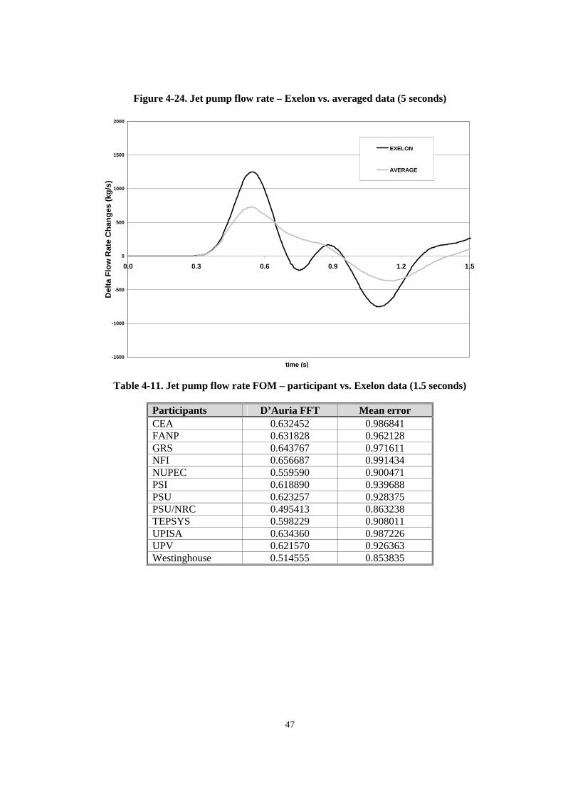
47

Figure 4-24. Jet pump flow rate – Exelon vs. averaged data (5 seconds)

-1500

-1000

-500

0

500

1000

1500

2000

0.0 0.3 0.6 0.9 1.2 1.5

time (s)

Del

taF

low

Rat

eC

han

ges

(kg

/s)

EXELON

AVERAGE

Table 4-11. Jet pump flow rate FOM – participant vs. Exelon data (1.5 seconds)


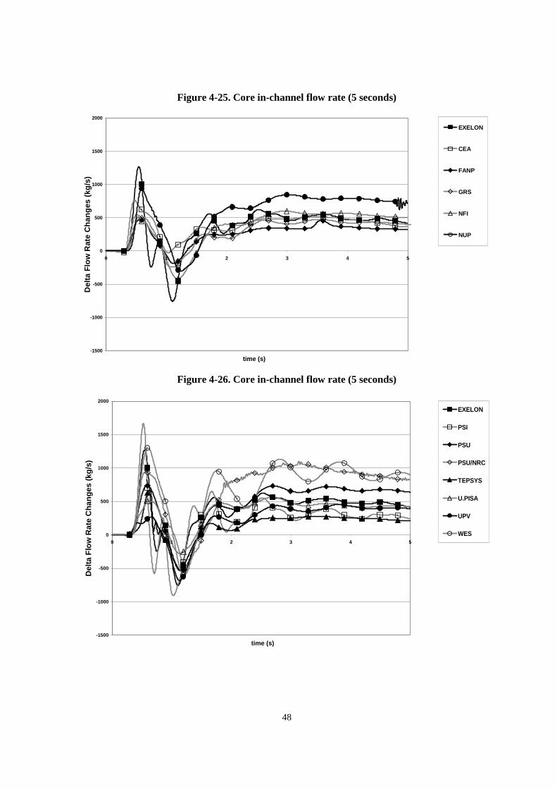
48

Figure 4-25. Core in-channel flow rate (5 seconds)

-1500

-1000

-500

0

500

1000

1500

2000

0 1 2 3 4 5

time (s)

Del

taF

low

Rat

eC

han

ges

(kg

/s)

EXELON

CEA

FANP

GRS

NFI

NUP

Figure 4-26. Core in-channel flow rate (5 seconds)

-1500

-1000

-500

0

500

1000

1500

2000

0 1 2 3 4 5

time (s)

Del

taF

low

Rat

eC

han

ges

(kg

/s)

EXELON

PSI

PSU

PSU/NRC

TEPSYS

U.PISA

UPV

WES

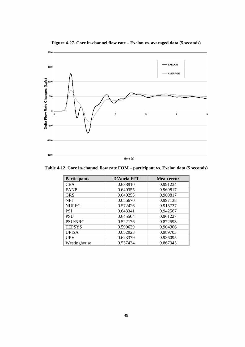
49

Figure 4-27. Core in-channel flow rate – Exelon vs. averaged data (5 seconds)

-1500

-1000

-500

0

500

1000

1500

2000

0 1 2 3 4 5

time (s)

Del

taF

low

Rat

eC

han

ges

(kg

/s)

EXELON

AVERAGE

Table 4-12. Core in-channel flow rate FOM – participant vs. Exelon data (5 seconds)


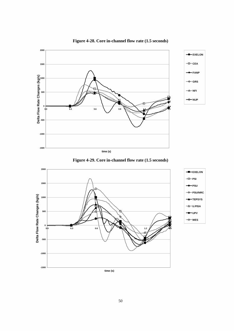
50

Figure 4-28. Core in-channel flow rate (1.5 seconds)

-1500

-1000

-500

0

500

1000

1500

2000

0.0 0.3 0.6 0.9 1.2 1.5

time (s)

Del

taF

low

Rat

eC

han

ges

(kg

/s)

EXELON

CEA

FANP

GRS

NFI

NUP

Figure 4-29. Core in-channel flow rate (1.5 seconds)

-1500

-1000

-500

0

500

1000

1500

2000

0.0 0.3 0.6 0.9 1.2 1.5

time (s)

Del

taF

low

Rat

eC

han

ges

(kg

/s)

EXELON

PSI

PSU

PSU/NRC

TEPSYS

U.PISA

UPV

WES

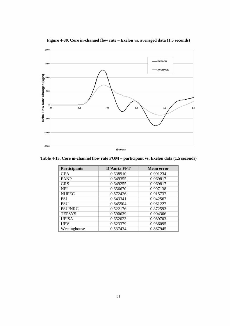
51

Figure 4-30. Core in-channel flow rate – Exelon vs. averaged data (1.5 seconds)

-1500

-1000

-500

0

500

1000

1500

2000

0.0 0.3 0.6 0.9 1.2 1.5

time (s)

Del

taF

low

Rat

eC

han

ges

(kg

/s)

EXELON

AVERAGE

Table 4-13. Core in-channel flow rate FOM – participant vs. Exelon data (1.5 seconds)


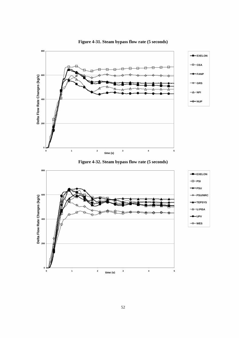
52

Figure 4-31. Steam bypass flow rate (5 seconds)

0

200

400

600

800

0 1 2 3 4 5time (s)

Del

taF

low

Rat

eC

han

ges

(kg

/s)

EXELON

CEA

FANP

GRS

NFI

NUP

Figure 4-32. Steam bypass flow rate (5 seconds)

0

200

400

600

800

0 1 2 3 4 5time (s)

Del

taF

low

Rat

eC

han

ges

(kg

/s)

EXELON

PSI

PSU

PSU/NRC

TEPSYS

U.PISA

UPV

WES

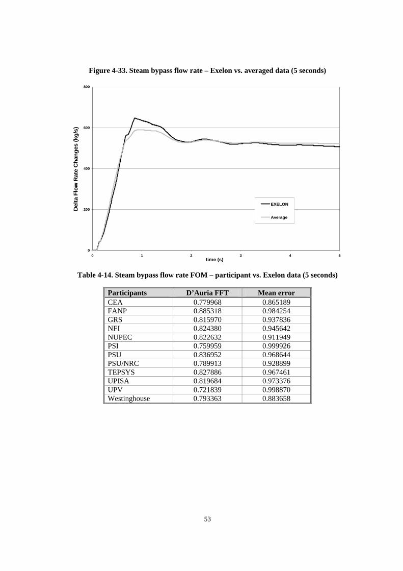
53

Figure 4-33. Steam bypass flow rate – Exelon vs. averaged data (5 seconds)

0

200

400

600

800

0 1 2 3 4 5time (s)

Del

taF

low

Rat

eC

han

ges

(kg

/s)

EXELON

Average

Table 4-14. Steam bypass flow rate FOM – participant vs. Exelon data (5 seconds)


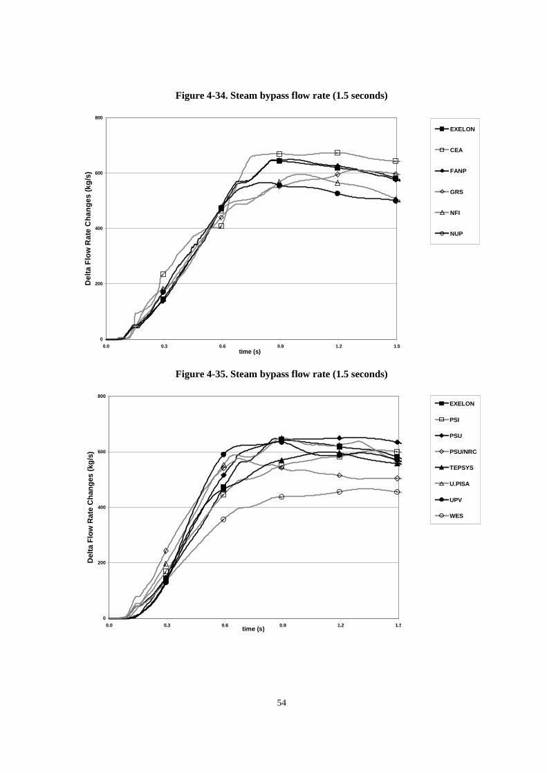
54

Figure 4-34. Steam bypass flow rate (1.5 seconds)

0

200

400

600

800

0.0 0.3 0.6 0.9 1.2 1.5time (s)

Del

taF

low

Rat

eC

han

ges

(kg

/s)

EXELON

CEA

FANP

GRS

NFI

NUP

Figure 4-35. Steam bypass flow rate (1.5 seconds)

0

200

400

600

800

0.0 0.3 0.6 0.9 1.2 1.5time (s)

Del

taF

low

Rat

eC

han

ges

(kg

/s)

EXELON

PSI

PSU

PSU/NRC

TEPSYS

U.PISA

UPV

WES

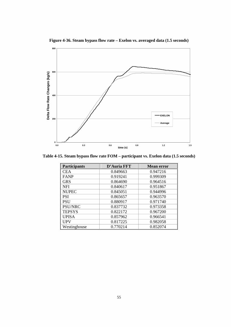
55

Figure 4-36. Steam bypass flow rate – Exelon vs. averaged data (1.5 seconds)

0

200

400

600

800

0.0 0.3 0.6 0.9 1.2 1.5time (s)

Del

taF

low

Rat

eC

han

ges

(kg

/s)

EXELON

Average

Table 4-15. Steam bypass flow rate FOM – participant vs. Exelon data (1.5 seconds)


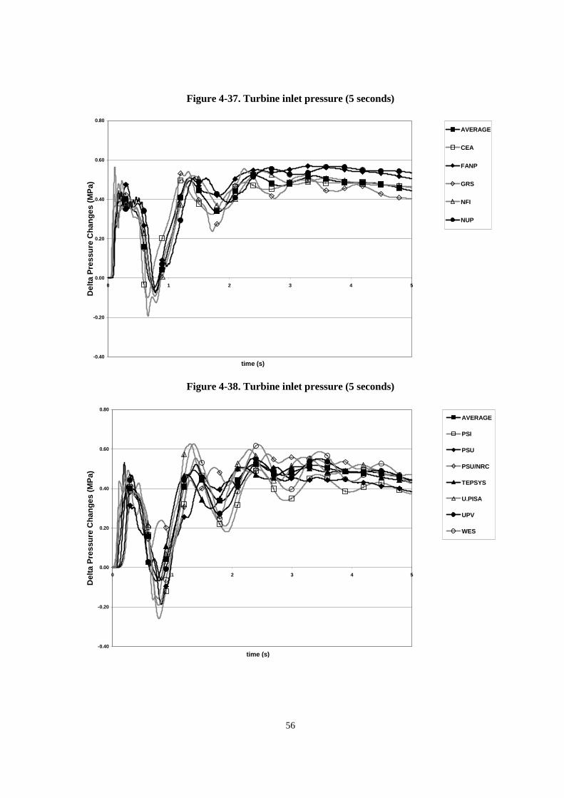
56

Figure 4-37. Turbine inlet pressure (5 seconds)

-0.40

-0.20

0.00

0.20

0.40

0.60

0.80

0 1 2 3 4 5

time (s)

Del

taP

ress

ure

Ch

ang

es(M

Pa)

AVERAGE

CEA

FANP

GRS

NFI

NUP

Figure 4-38. Turbine inlet pressure (5 seconds)

-0.40

-0.20

0.00

0.20

0.40

0.60

0.80

0 1 2 3 4 5

time (s)

Del

taP

ress

ure

Ch

ang

es(M

Pa)

AVERAGE

PSI

PSU

PSU/NRC

TEPSYS

U.PISA

UPV

WES

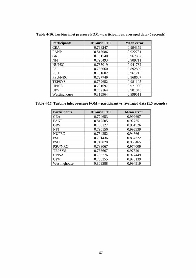
57

Table 4-16. Turbine inlet pressure FOM – participant vs. averaged data (5 seconds)


Table 4-17. Turbine inlet pressure FOM – participant vs. averaged data (1.5 seconds)


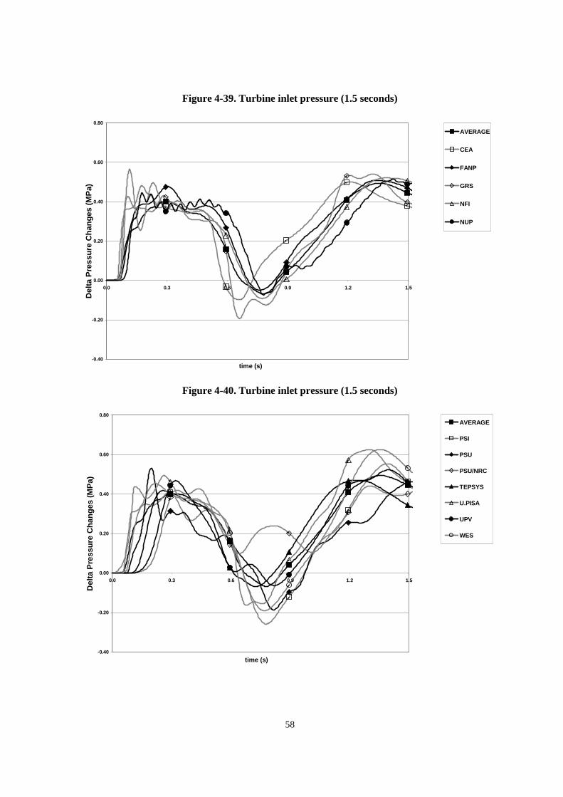
58

Figure 4-39. Turbine inlet pressure (1.5 seconds)

-0.40

-0.20

0.00

0.20

0.40

0.60

0.80

0.0 0.3 0.6 0.9 1.2 1.5

time (s)

Del

taP

ress

ure

Ch

ang

es(M

Pa)

AVERAGE

CEA

FANP

GRS

NFI

NUP

Figure 4-40. Turbine inlet pressure (1.5 seconds)

-0.40

-0.20

0.00

0.20

0.40

0.60

0.80

0.0 0.3 0.6 0.9 1.2 1.5

time (s)

Del

taP

ress

ure

Ch

ang

es(M

Pa)

AVERAGE

PSI

PSU

PSU/NRC

TEPSYS

U.PISA

UPV

WES

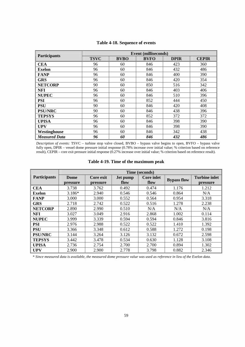
59

Table 4-18. Sequence of events

Event (milliseconds)ParticipantsTSVC BVBO BVFO DPIR CEPIR

CEA 96 60 846 423 360Exelon 96 60 846 432 486FANP 96 60 846 400 390GRS 96 60 846 420 354NETCORP 90 60 850 516 342NFI 96 60 846 403 406NUPEC 96 60 846 510 396PSI 96 60 852 444 450PSU 90 60 846 420 408PSU/NRC 90 60 846 438 396TEPSYS 96 60 852 372 372UPISA 96 60 846 398 390UPV 96 60 846 398 390Westinghouse 96 60 846 342 438Measured Data 96 60 846 432 486

Description of events: TSVC – turbine stop valve closed, BVBO – bypass valve begins to open, BVFO – bypass valvefully open, DPIR – vessel dome pressure initial response (0.78% increase over initial value; % criterion based on referenceresult), CEPIR – core exit pressure initial response (0.27% increase over initial value; % criterion based on reference result).

Table 4-19. Time of the maximum peak

Time (seconds)Participants Dome

pressureCore exitpressure

Jet pumpflow

Core inletflow

Bypass flow Turbine inletpressure

CEA 3.738 3.762 0.492 0.474 1.176 1.212Exelon 13.186* 2.940 0.546 0.546 0.864 N/AFANP 3.000 3.000 0.552 0.564 0.954 3.318GRS 2.718 2.742 0.522 0.516 1.278 2.238NETCORP 2.890 2.990 0.510 N/A N/A N/ANFI 3.027 3.049 2.916 2.868 1.002 0.114NUPEC 3.999 3.339 0.594 0.594 0.846 3.816PSI 2.976 2.988 0.522 0.522 1.410 1.392PSU 3.366 3.348 0.612 0.588 1.272 0.198PSU/NRC 3.144 3.264 3.126 3.132 0.672 2.598TEPSYS 3.442 3.478 0.534 0.630 1.128 3.108UPISA 2.736 2.754 2.700 2.700 0.894 1.302UPV 2.900 2.900 2.778 3.798 0.882 2.346

* Since measured data is available, the measured dome pressure value was used as reference in lieu of the Exelon data.

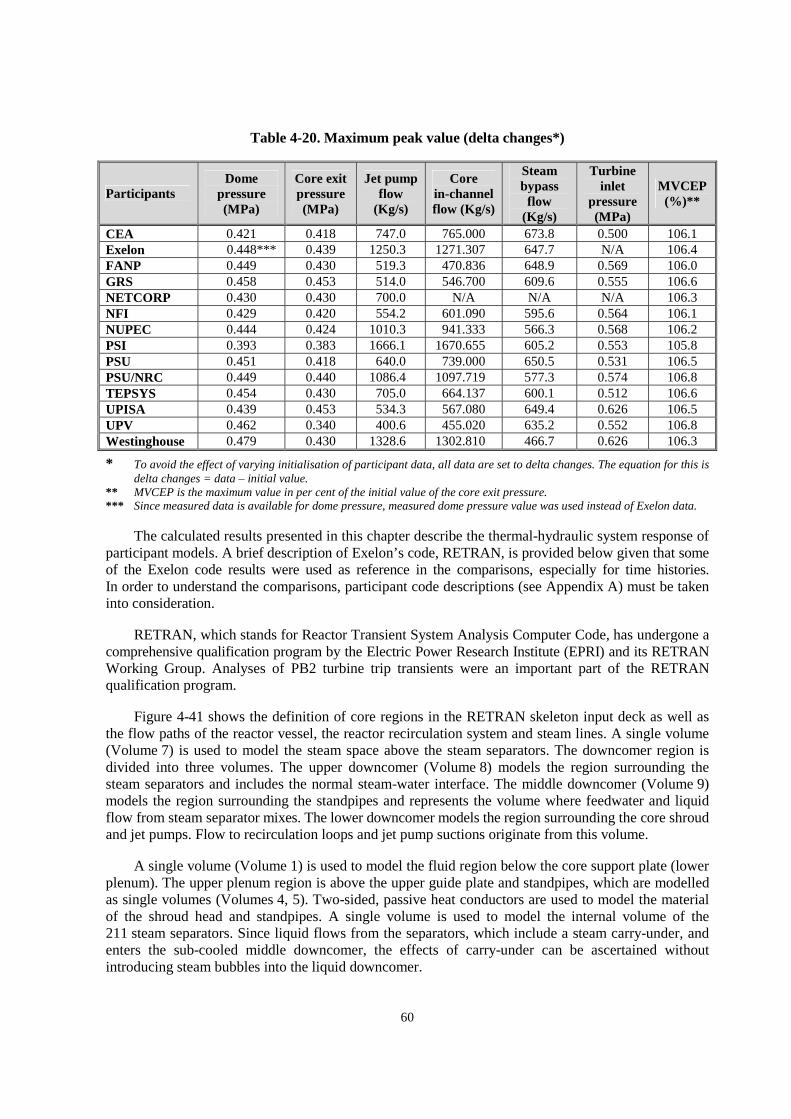
60

Table 4-20. Maximum peak value (delta changes*)

ParticipantsDome

pressure(MPa)

Core exitpressure(MPa)

Jet pumpflow

(Kg/s)

Corein-channelflow (Kg/s)

Steambypass

flow(Kg/s)

Turbineinlet

pressure(MPa)

MVCEP(%)**

CEA 0.421 0.418 747.0 765.000 673.8 0.500 106.1Exelon 1110.448*** 0.439 1250.31 1271.3071 647.7 N/A 106.4FANP 0.449 0.430 519.3 470.836 648.9 0.569 106.0GRS 0.458 0.453 514.0 546.700 609.6 0.555 106.6NETCORP 0.430 0.430 700.0 N/A N/A N/A 106.3NFI 0.429 0.420 554.2 601.090 595.6 0.564 106.1NUPEC 0.444 0.424 1010.31 941.333 566.3 0.568 106.2PSI 0.393 0.383 1666.11 1670.6551 605.2 0.553 105.8PSU 0.451 0.418 640.0 739.000 650.5 0.531 106.5PSU/NRC 0.449 0.440 1086.41 1097.7191 577.3 0.574 106.8TEPSYS 0.454 0.430 705.0 664.137 600.1 0.512 106.6UPISA 0.439 0.453 534.3 567.080 649.4 0.626 106.5UPV 0.462 0.340 400.6 455.020 635.2 0.552 106.8Westinghouse 0.479 0.430 1328.61 1302.8101 466.7 0.626 106.3

* To avoid the effect of varying initialisation of participant data, all data are set to delta changes. The equation for this isdelta changes = data – initial value.

** MVCEP is the maximum value in per cent of the initial value of the core exit pressure.*** Since measured data is available for dome pressure, measured dome pressure value was used instead of Exelon data.

The calculated results presented in this chapter describe the thermal-hydraulic system response ofparticipant models. A brief description of Exelon’s code, RETRAN, is provided below given that someof the Exelon code results were used as reference in the comparisons, especially for time histories.In order to understand the comparisons, participant code descriptions (see Appendix A) must be takeninto consideration.

RETRAN, which stands for Reactor Transient System Analysis Computer Code, has undergone acomprehensive qualification program by the Electric Power Research Institute (EPRI) and its RETRANWorking Group. Analyses of PB2 turbine trip transients were an important part of the RETRANqualification program.

Figure 4-41 shows the definition of core regions in the RETRAN skeleton input deck as well asthe flow paths of the reactor vessel, the reactor recirculation system and steam lines. A single volume(Volume 7) is used to model the steam space above the steam separators. The downcomer region isdivided into three volumes. The upper downcomer (Volume 8) models the region surrounding thesteam separators and includes the normal steam-water interface. The middle downcomer (Volume 9)models the region surrounding the standpipes and represents the volume where feedwater and liquidflow from steam separator mixes. The lower downcomer models the region surrounding the core shroudand jet pumps. Flow to recirculation loops and jet pump suctions originate from this volume.

A single volume (Volume 1) is used to model the fluid region below the core support plate (lowerplenum). The upper plenum region is above the upper guide plate and standpipes, which are modelledas single volumes (Volumes 4, 5). Two-sided, passive heat conductors are used to model the materialof the shroud head and standpipes. A single volume is used to model the internal volume of the211 steam separators. Since liquid flows from the separators, which include a steam carry-under, andenters the sub-cooled middle downcomer, the effects of carry-under can be ascertained withoutintroducing steam bubbles into the liquid downcomer.

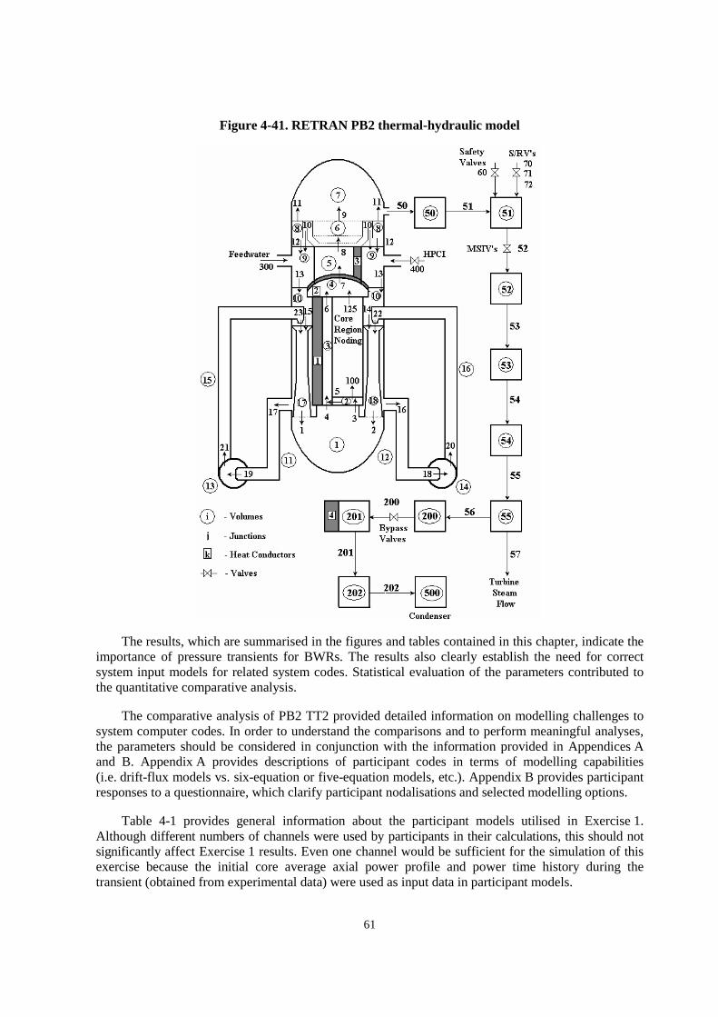
61

Figure 4-41. RETRAN PB2 thermal-hydraulic model

The results, which are summarised in the figures and tables contained in this chapter, indicate theimportance of pressure transients for BWRs. The results also clearly establish the need for correctsystem input models for related system codes. Statistical evaluation of the parameters contributed tothe quantitative comparative analysis.

The comparative analysis of PB2 TT2 provided detailed information on modelling challenges tosystem computer codes. In order to understand the comparisons and to perform meaningful analyses,the parameters should be considered in conjunction with the information provided in Appendices Aand B. Appendix A provides descriptions of participant codes in terms of modelling capabilities(i.e. drift-flux models vs. six-equation or five-equation models, etc.). Appendix B provides participantresponses to a questionnaire, which clarify participant nodalisations and selected modelling options.

Table 4-1 provides general information about the participant models utilised in Exercise 1.Although different numbers of channels were used by participants in their calculations, this should notsignificantly affect Exercise 1 results. Even one channel would be sufficient for the simulation of thisexercise because the initial core average axial power profile and power time history during thetransient (obtained from experimental data) were used as input data in participant models.

62

Correct modelling of initial steady state is important – the TT2 test has been initiated from thesteady state conditions of the EOC 2. Participant results have shown excellent agreement for steadystate parameters. Although CEA, NETCORP and TEPSYS predictions seem to deviate more noticeablyfrom the reference results presented in Figures 4-1 and 4-2, the maximum deviation for the core inletenthalpy is less than 0.7% and less than 23% for the core pressure drop. The inlet enthalpy usuallydepends on the amount of steam carry-under from the separators. The transient response of the systemis very sensitive to separator modelling because this affects the initial location of the bulk boilingin core channels. The good agreement obtained in the core inlet enthalpy predictions is encouragingfor the participants to perform further analyses. The accuracy of the core pressure drop calculationsis affected by the predictions of the inlet enthalpy, which is related to the modelling of steamseparators/dryers and loss coefficients in the vessel and channels. Since the inlet enthalpy predictionsagree quite well, the observed discrepancies in the pressure drop predictions may come fromparticipant models other than the separator models.

The most challenging part of the steady state analysis is the prediction of the void fractiondistribution. This prediction depends on the modelling of core channels, vessel levels, steam dryers/separators, jet pumps and recirculation loops, and also depends on the features of the participantsystem codes. With all these challenges in mind, one can consider that the core average axial voidfraction distribution results agree very well. An interesting observation can be made regardingFigure 4-5, which shows very good agreement of the average result over all participants’ predictionsas compared to the Exelon results. Among the void fraction results, only the FANP prediction exhibitsdeviation from the reference result as shown in Figure 4-3. The reason may come from the calculationof the channel and vessel loss coefficients. Most of the results have shown slight differences at theaxially lower (bottom) part of the core, such as PSI’s prediction (Figure 4-4). Since there is noneutronic feedback for this exercise, the slight deviations may be explained by participants’ differentthermal-hydraulic flow and heat transfer models and especially sub-cooled boiling models.

In summary, steady state simulation of large systems is very difficult and requires extensive workon each component’s model. In addition, correct simulation is necessary of the control phenomena ininput models, such as water level control, recirculation pump speed, jet pump flows, feedwater flowand steam line pressure.

The calculated transient results and the comparisons presented in this chapter not only provide anopportunity to understand the phenomena behind the turbine transient tests but also to engage incomprehensive testing and examination of the capability of participant codes to simulate suchtransients. During the benchmark workshops, three important decisions were made by the participantsrelated to the comparative analysis of the time histories: 1) to analyse the time histories of deltachanges (instead of absolute parameter values) in order to avoid the impact of initial steady statedisagreements; 2) to provide two comparisons for 1.5 s and for 5 s; and 3) to provide two FOM estimatesbased on two different methods (FFT and ME).

In general, it was demonstrated that the steam bypass line has a strong interaction with the mainsteam line and the steam bypass line’s impact on the pressure responses depends on the relative positionof the TSV and BPV. It was observed that an acoustical pressure wave (oscillation) can exist in thereactor main steam piping due to the combined compressibility and momentum effects in the steamline. The fundamental mode of the acoustical pressure oscillation is strongly excited as a result of turbinetrip, which causes a sharp initial pressure rise in the reactor as the first pressure wave enters the reactorvessel. In addition, the fundamental acoustical mode propagates in the main steam piping, entering thereactor vessel and passing through the steam separators into the reactor core with relatively littleattenuation. All of these physical facts can be seen in participant results (Figures 4-7 through 4-40).

63

During analysis of the results for the first exercise, it was obvious that the sources of deviations inparticipant predictions came from the differences in modelling the two key parameters – pressureresponse and core flow response. Accurate prediction of the pressure response depends on the numberof models used by a given code. Models include: the steam line model (requires adequate nodalisationand treatment of momentum effects), the steam bypass system model and the steam separator model(requires proper treatment of steam separator inlet inertia and non-equilibrium effects at steam-watersurfaces). Prediction of core flow response is sensitive to the jet pump model used (requires properrepresentation of the dynamic response of flow-to-pressure) and the core exit/separator region model(requires proper representation of the dynamic response of two-phase flow).

Figures 4-7 through 4-18 and Tables 4-6 through 4-9 present the comparative analysis of participantvessel dome pressure and core exit pressure results with the reference data. In principle, the results arein good agreement. In particular, the good agreement in the times of occurrence of the initial riseindicates that the time effects (delays, rise times and frequencies) are modelled well. In addition, theamplitudes of the pressures are generally in good agreement. The discrepancies can be attributed to theshortcomings of the code models. For example, improving the slip model may increase the accuracy ofthe results because the reactor pressure vessel may have a larger liquid inventory and lower steaminventory, which tend to produce higher pressures.

If Tables 4-6 through 4-9 are analysed together, it can be concluded that some participantpredictions agree well with the reference solutions in the first 1.5 seconds of the transient while otherparticipant predictions agree well in the later part of the transient. The reason for this may be explainedin the following statements. The overall behaviour of the pressure is mostly affected by the transientflow rate of steam through the turbine stop valves and bypass valves. Simulation of the opening andclosing of the valves and nodalisation of the steam lines play an important role in the calculations. Thediscrepancies seen in the latter phases of these curves may arise from depressurisation rate mechanisms(e.g. critical flow models and steam formation models).

Participant results for jet pump flow rate (total core flow rate) and core in-channel flow rate aregenerally consistent as shown in Figures 4-19 through 4-30 and in Tables 4-10 through 4-13. Althoughthe submitted results in the figures seem to have great deviations when compared with the referencedata, it should be noted that the illustrated results are based on delta changes (explained in Chapter 3).If the initial values of the flow rates (such as 10 445 kg/s for total core rate) are considered, then themaximum deviation is evaluated at less than 10%.

Discrepancies in flow rate responses can be analysed in 2 sections – deviations before 1.5 secondsand after 1.5 seconds. Most problematic in the period before 1.5 seconds were predictions of peak timesand peak amplitudes as well as the simulation of wave propagation. The best agreement with referenceresults in the flow rate prediction was achieved by the PSI results. As described in Appendix A, PSIused RETRAN-3D, which is based on the code RETRAN (used by Exelon for reference calculations).

In the latter phases of the jet pump flow rate and core in-channel flow rate figures, the NUPEC,PSU/NRC and Westinghouse predictions were ~3-5% higher than the reference solution. The mostprobable reason for this disagreement is the input model (if the effect of the core bypass flow modelon the core flows is considered). In most models, the core bypass flow is directly related to the totalcore flow. For instance, a decrease in core bypass flow causes an increase in total core flow rate.

Although steam bypass modelling is one of the most challenging parts of the exercise, thesubmitted results have shown that participant models can simulate steam bypass flow successfully.The submitted results agree well as shown by Figures 4-31 through 4-36 and by Tables 4-14, 4-15.The predictions shown in the figures deviated at the peak time and especially at the end of the transient.

64

Assumptions used in modelling the phenomena between the flow through steam bypass valve and thevalve opening area had a great effect on the results. In addition, the predictions were very importantbecause the bypass flow rate itself greatly influenced peak pressures.

Predictions of the participant models are also affected by the choice of bypass piping heat transferoptions [10]. As hot steam enters the bypass valves, significant heat is transferred to the cold pipingwalls due to the large temperature gradient. This event causes slower pressurisation of bypass piping,which increases the affects of the critical flow through the bypass valve. The heat transfer to the pipewalls causes an increase of the flow rate until walls reach the steam temperature. In most cases, pipesare cold (i.e. their temperatures are close to the condenser temperature); however, there is evidencethat the piping walls remain at a high temperature for some time after steam bypass opening. Since theTT2 event followed TT1, during the opening of the bypass valves the heat transfer to the walls may benegligible [7]. Finally, it was shown that the transient flow phenomena in the steam bypass system areof great importance.

As a parameter for the time histories, turbine inlet pressure predictions were compared with theaverage result. All results were in quite good agreement. Some slight deviations on the initial pressureresponse were possibly a result of the differences in the action of TSV modelling. The modelling ofthis action affects the prediction of certain time effects such as delays, rise times and frequencies.

The remarkable overall good agreement between reference and participant results for time historiesraised confidence in the participants’ system codes as well as in the developed system models. Moreover,the excellent agreement, which is illustrated in Figures 4-9, 4-12, 4-15, 4-18, 4-21, 4-24, 4-27, 4-30,4-33, 4-36 and 4-39, between average and reference results not only indicated the success of thisbenchmark but also encouraged participants to take part in the remaining exercises.

In addition to time histories, sequence of events, maximum peak times for time histories andmaximum peak values can be found in Tables 4-18, 4-19 and 4-20. Although participant event timingsfor TSVC, BVBO and BVFO were perfect as shown in Table 4-18, initial responses had slightdifferences. In parallel, time and maximum peaks presented in Tables 4-19 and 4-20 had discrepancies.The possible reasons for these discrepancies were explained in the above paragraphs.

In conclusion, the results of the first exercise verified the participants’ system codes and systemmodels, and contributed to gaining a more in-depth knowledge of the capabilities of these codes.Developing a more in-depth knowledge of coupled computer code systems is important because 3-Dkinetic/thermal-hydraulic codes will play a critical role in the future of nuclear analysis. Since thepurpose of this exercise was to initialise and test the thermal-hydraulic system model responses, thischapter proved that this exercise laid the foundation for conducting other benchmark exercises in aconsistent and systematic way.

65

Chapter 5

CONCLUSIONS

In order to meet the objectives for the validation of best-estimate coupled codes, a systematic approach was introduced to evaluate the turbine trip transient. Such codes use separate temporal and spatial models as well as numerical methods for core neutronics, core thermal-hydraulics and system thermal-hydraulic simulations. Therefore, the validation of the codes should include testing these models for the defined transient for a given type of reactor (BWR in this case) as separate exercises of the overall benchmark.

The ultimate goal is to enable participants to initiate and verify these models before focusing on the major objective, which is the testing of coupling methodologies in terms of numerics, temporal and spatial mesh overlays. This approach allows one to evaluate in a more consistent way the modelling of combined effects (neutronics/thermal-hydraulics as well as core/plant interactions) by removing the uncertainties introduced with separate models.

In order to perform such a comprehensive validation of coupled codes, a multi-level methodology is employed. This includes the application of three exercises, the evaluation of different steady states and the simulation of different transient scenarios.

To summarise this work, Exercise 1 of the BWR TT benchmark was discussed in detail. The results of this benchmark problem were intended to assist in the understanding of the behaviour of next generation computer codes. Overall, this benchmark has been well-accepted internationally, with 14 participants from 8 countries participating in the first exercise. The results submitted by participants of Exercise 1 were used to make comparisons and a subsequent statistical analysis. This information encompassed several types of data for thermal-hydraulic parameters at the initial steady state conditions and throughout the turbine trip transient. These included: integral parameters, 1-D axial distributions and time histories.

Due to the sensitive nature of this transient to small variations in initial parameters, the participants were advised to follow the final specifications as closely as possible. In order to avoid possible misinterpretations, the benchmark team provided further clarifications before the final results were submitted. The motivation behind such clarifications was to narrow down as much as possible the modelling differences for the initial steady state conditions as well as for the transient scenario. This strategy helped to obtain a cluster of solutions to be used as a basis for further comparative analysis.

A detailed assessment of the differences between calculated results submitted by the participants for this exercise was presented in Chapter 4 of this report. Overall, the participant results for integral parameters, core-averaged axial distributions and core-averaged time histories were in good agreement with reference solutions, especially considering the approximations in some participant models, the uncertainties of some system parameters and the difficulties in interpreting some of the measured responses. This is important from the fluid phenomena point of view because pressure and flow waves play an important role in the early phase of the response to a turbine trip.

66

Since core inlet enthalpy is highly sensitive to core inlet temperature, the submitted results were accepted as being in very good agreement. Besides, participant predictions for the core pressure drop were quite close to the reference value if complexities of such system models were taken into account. In the void fraction results, deviations were mostly observed in the lower (bottom) part of the core because of differences in the participants’ sub-cooled boiling models. However, the average distribution calculated from the participants’ submitted results almost matched the reference solution.

Generally, time history results and transient single values were in very good agreement with the reference data. Although some parameters seemed to have deviations, surprisingly, the average values matched the reference solution well. We observed that more than 10 submitted sets of data could make the comparative analysis meaningful in terms of the statistical approach.

In the time history comparisons, the deviations were mostly observed within the first 1.5 second time period after the start of the transient. Since power was provided as a function of time (to eliminate the impact of neutronic feedback effects), the deviations in the first 1.5 seconds may have come from the computer code control capabilities or from the approximations of participant models used in this transient (especially simulating the bypass phenomena).

It was demonstrated that Exercise 1 fulfilled its objective, namely, to help the participants initialise and test thermal-hydraulic system models to be used later in Exercise 3 (coupled 3-D neutron kinetics/system thermal-hydraulic calculations of PB2 TT2). In addition, the participants utilised Exercise 1 to perform a number of sensitivity studies on different modelling and numerical issues. Such investigations were aimed toward evaluation of impact of the following effects and parameters:

� Thermal-hydraulic modelling issues: Turbine bypass line modelling; nodalisation of vessel, steam line and steam separator region; TSV position and steam mass flow modelling; thermal-hydraulic model – number of equations; void fraction model; steam separator inertia; and jet pump modelling.

� Thermal-hydraulic key parameters: Feedwater temperature; jet pump parameters; void fraction in the bulk water (carry-under); core outlet pressure; active core pressure loss; core inlet temperature; core inlet mass flow without bypass flow; sub-cooling; void generation rate; and gas gap conductance.

� Timestep size: Fixed timestep of 6 ms versus using a variable timestep algorithm with a maximum timestep size imposed.

Exercise 1 provided the opportunity to study the impact of different thermal-hydraulic models on code predictions and to identify the key parameters for modelling a TT transient. This in turn allowed the evaluation of key parameters through the performance of sensitivity studies, which allowed the participants to develop a more in-depth knowledge of the capabilities of current generation best-estimate thermal-hydraulic system codes.

67

REFERENCES

[1] Ivanov, K.N., T. Beam, A. Baratta, A. Irani, N. Trikouros, PWR MSLB Benchmark – Final Specifications, Nuclear Energy Agency, NEA/NSC/DOC(97)15, October 1997.

[2] Solis, J., K.N. Ivanov, B. Sarikaya, A. Olson, K. Hunt, Boiling Water Reactor Turbine Trip (TT) Benchmark Volume I: Final Specifications, Nuclear Energy Agency of the Organisation for Co-operation and Development, NEA/NSC/DOC(2001)1, June 2001.

[3] “Transient and Stability Tests at Peach Bottom Atomic Power Station Unit 2 at End of Cycle 2”, General Electric Company/Nuclear Energy Engineering Division, NP-564, Research Project 1020-I, Topical Report, June 1978.

[4] Larsen, N.H., “Core Design and Operating Data for Cycles 1 and 2 of Peach Bottom 2”, EPRI NP-563, June 1978.

[5] Carmichael, L.A., R.O. Niemi, “Transient and Stability Tests at Peach Bottom Atomic Power Station Unit 2 at End of Cycle 2”, EPRI NP-564, June 1978.

[6] Hornyik, K., J.A. Naser, “RETRAN Analysis of the Turbine Trip Tests at Peach Bottom Atomic Power Station Unit 2 at the End of Cycle 2”, EPRI NP-1076-SR Special Report, April 1979.

[7] Olson, A.M., “Methods for Performing BWR System Transient Analysis”, Philadelphia Electric Company, Topical Report PECo-FMS-0004-A (1988).

[8] Kuntz, R.F., G.F. Kasmala, J.H. Mahaffy, “Automated Code Assessment Program: Technique Selection and Mathematical Prescription”, Applied Research Laboratory, Pennsylvania State University, Letter Report 3 to US NRC, April 1998.

[9] Cubic_spline for Excel workbook, SRS1 Software, February 2003. Available at the website http://www.srs1software.com.

[10] Akdeniz, B., K.N. Ivanov, “Analysis and Sensitivity Studies of Exercise 1 of OECD/NRC BWR TT Benchmark”, TANSAO 87 (2002).

[11] Ambrosini, W., R. Bovalini, F. D’Auria, “Evaluation of Accuracy of Thermal-hydraulics Code Calculations”, Energia Nucleare, Vol. 7, No. 2 (1990).

69

Appendix A

DESCRIPTION OF COMPUTER CODES USED FOR ANALYSISOF EXERCISE 1 OF THE NEA-NRC BWR TT BENCHMARK

71

CATHARE (CEA, France)

The development of the CATHARE code was initiated in 1979 [1]. Code objectives include:

• Perform safety analyses with best-estimate calculations of thermal-hydraulic transients inpressurised water reactors.

• Quantify the conservative analysis margin.

• Investigate plant operating procedures and accident management.

• Evaluate usage as plant analyser in full-scope training simulator providing real-time calculation.

The code is based on a two-fluid six-equation model. The presence of non-condensable gases canbe modelled by one to four additive transport equations. The code is able to model any kind ofexperimental facility or PWR, and is usable for other reactors (fusion reactor, BWRs, etc.)

The CATHARE code applications have been extended by coupling with other codes:

• Three-dimensional neutronics code – CRONOS [2].

• Core thermal-hydraulic code (component code) – FLICA [3].

• Severe accident code – ICARE2 [4].

CATHARE Main features

CATHARE has a modular structure. The modules are:

• One-dimensional module to describe pipe flow.

• Volume module, which is a two-node module.

• Three-dimensional module to describe multi-dimensional effects in the vessel.

To complete the modelling of the circuits, sub-modules can be connected to the main modules(e.g. the multi-layer wall module), the point neutronics module, valves, safety valves, check valves,flow limiters, boundary conditions, etc.

Physical description

All modules use the two-fluid model to describe steam-water flows and four non-condensablegases that may be transported. Both thermal and mechanical non-equilibrium of the two phases aredescribed.

All kinds of two-phase flow patterns are modelled [5]. Heat transfer with wall structures and fuelrods are calculated, taking into account all heat transfer processes: natural and forced convection withliquid or gas, sub-cooled and saturated nucleate boiling, critical heat flux, film condensation for effectsof non-condensable gases, etc.

72

The range of parameters is rather large: pressure from 0.1-25 MPa, gas temperature from20-2 000°C, fluid velocities up to supersonic conditions and duct hydraulic diameters from 0.01-0.75m.

System of equations

Mass, momentum and energy equations are established for any CATHARE module. They arewritten for each phase. They are derived from exact local instantaneous equations, using somesimplification through physical assumptions as well as time and space averaging procedures. One tofour transport equations can be added when non-condensable gases are present.

Physical models are required to close the system of equations for CATHARE. Closurerelationships concern mass, momentum and energy exchanges between phases and between each phaseand the wall. As much as possible, physical closure laws are developed on an experimental basis.

Numerical scheme and solution procedure

The numerical method in the CATHARE code uses a first order finite volume/finite differencescheme with a staggered mesh and donor cell principle. The time discretisation varies from the fullyimplicit discretisation used in the 0-D and 1-D modules to the semi-implicit scheme used in the 3-Dmodule. Wall conduction is implicitly coupled to hydraulic calculations.

The non-linear system of equations is solved by a Newton-Raphson iterative method. In the lastversion of CATHARE (v1.5), the solution can be distributed over several processors in order to reducethe CPU time by parallel computing.

References

[1] Houdayer, G., J.C Rousseau, B. Brun, “The CATHARE Code and its Qualification onAnalytical Experiments”, 10th Water Reactor Safety Research Information, Washington,October 1982.

[2] Lautard, J.J., S. Loubiere, C. Magnaud, “CRONOS: A Modular Computational System forNeutronic Core Calculations”, IAEA meeting, Cadarache, France (1990).

[3] Toumi, I., A. Bergeron, D. Gallo, E. Royer, D. Caruge, “FLICA4: A Three-dimensionalTwo-phase Flow Computer Code with Advanced Numerical Methods for Nuclear Applications”,Nuclear Engineering and Design, 200, 139-155 (2000).

[4] Guillard, V., F. Fhicot, P. Boudier, M. Parent, R. Roser, “ICARE/CATHARE Coupling:Three-dimensional Thermal-hydraulics of Severe LWR Accidents”, ICONE9, Nice Acropolis,France (2001).

[5] Bestion, D., “The Physical Closure Laws in the CATHARE Code”, Nuclear Engineering andDesign, Vol. 124, pp. 229-245 (1990).

73

S-RELAP5 (FANP, Germany)

S-RELAP5 is the standard tool of FRAMATOME ANP for the investigation of accident scenariosin nuclear power plants, both of PWR and BWR. The range of applications covers LBLOCA on theone end and reactor transients on the other end. S-RELAP5 includes all features of the RELAP5 codefamily. It is a highly modular code where the user defines the granularity of the analysis by definingan appropriate noding scheme.

The hydraulic part of such a noding scheme includes a concatenation of hydraulic volumesconnected by junctions. In the case of a two-phase state in the hydraulic volume, thermalnon-equilibrium is assumed. The two-phase flow between the volumes is non-homogeneous; thecorresponding phasical velocities are determined by solving momentum equations. This approachrequires the definition of local static pressure, with the pressure gradient being the source ofmovement for each phase. Thermal properties as densities or internal energies are locally defined.In S-RELAP5, flow maps and heat transfer modes are defined; they allow for the application ofconstitutive relations as inter-phasical shear or heat transfer coefficients, which depend on them. Ahighly sophisticated numerical solution scheme allows for the consideration of hydraulic systems withup to 500 hydraulic volumes. S-RELAP5 has a fully developed fuel model and a point kinetic model.

ATHLET (GRS, Germany)

The system code ATHLET is applied for analysis of behaviour of the whole plant under accidentconditions. It is a thermal fluid dynamic system code based on 1-D pipe components with a wide rangeof applications. The applications are comprised of anticipated and abnormal plant transients, small andintermediate leaks as well as large breaks in PWRs and BWRs. The code offers the possibility ofchoosing between different models of fluid dynamics. The two-phase flow can be described with up toa full six-equation model for mass, energy and momentum of both phases, including models fornon-condensables. A boron tracking model for single and two-phase flow has been implemented. Thecode structure is highly modular and allows for easy implementation of different physical models. Thebasic modules include: thermo-fluid dynamics, neutron kinetics, general control simulation moduleand numerical integration method FEBE. ATHLET provides a modular network approach for therepresentation of a thermal-hydraulic system. The possibility to implement connections among a groupof parallel channels in the reactor core allows for the modelling of cross flow inside the reactor core.

DNB/3D (NETCORP, USA)

DNB/3D is a FORTRAN 77 computer program that simulates the nuclear steam supply system ofa boiling water reactor under transient conditions. Geometry and system component options are providedto represent any of the current BWR designs. The major features of DNB/3D are as follows:

• Point, 1-D and 3-D neutronic kinetics models including Doppler, moderator density andcontrol rod feedback along with standard decay heat models. Initially, sub-critical cores canbe represented. A power forced option is also provided.

• Multi-node radial and axial coolant channels and fuel rods.

• Fixed nodalisation in the reactor vessel and steam lines.

• One-dimensional homogeneous equilibrium conservation of mass, energy and momentum.

74

• Mechanistic non-equilibrium flow quality or profile fit model option to represent slip with thecoolant channels.

• Steam line includes representation of the MSIV, turbine control and stop valves, RSV andsteam bypass valves.

• Method of characteristics used to solve conservation equations in the steam lines.

• Turbine representation.

• Structural metal components represented. Reactor protection and safety systems represented.

• Control systems represented. Complete self-initialisation of all components and models.

• Provisions to represent a wide variety of transient and accident scenarios. Flexible restartcapability. British or Sl input/output option.

TRAC-BF1 (NFI, Japan)

The code used in the first exercise is TRAC-BF1/MOD1. TRAC-BF1/COS3D is not used in thisexercise but in the others. TRAC-BF1 is a best-estimate transient analysis code for analysing the fullrange of postulated accidents in boiling water reactor systems and related facilities.

TRAC-BF1 (NUPEC, Japan)

NUPEC used the TRAC-BF1 code in the first exercise. TRAC-BF1 is the latest public domainBWR version of TRAC, which deals with thermal hydraulics, fuel heat transfer and plant system.Thermal-hydraulics utilises the two-fluid model that solves six balance equations of mass, momentumand energy for liquid and vapor phases. Two-phase flow in the core region is treated as 1-D parallelvertical flows. The heat transfer model solves 1-D radial heat conduction equations. Heat transfercoefficients at the cladding surface are subdivided into each flow regime. Material properties are basedon the code-installed MATPRO correlations. TRAC-BF1 has major BWR component modules: vessel,channel, separator/dryer, pump, pipe, valve, etc. The plant system can be composed of thesecomponent modules. The reactor pressure vessel is modelled with the vessel component in 3-Dcylindrical co-ordinates. Two numerical methods for thermal-hydraulic calculations are used. The firstis the standard finite differential method with staggered mesh, which is used for the space integrationof both fluid flow and heat conduction. The second is the time integration of fluid flow equations,which is performed by the semi-implicit scheme with the stability enhanced two-step (SETS) method.

RETRAN-3D (PSI, Switzerland)

Within the STARS project at PSI, the code environment for the coupled 3-D reactor-kinetics/thermal-hydraulics transient analyses of Swiss LWRs is based mainly on RETRAN-3D andCORETRAN for both PWR and BWR systems. (Note that other codes are used for specificapplications, e.g. RAMONA for BWR stability.) Both codes play distinct roles in this environment –RETRAN-3D is used for analysis of coupled 3-D core/plant system transients while CORETRAN is

75

used for core-only dynamic analysis. An important aspect is that both codes are based on an identicalneutronics algorithm, allowing usage of CORETRAN as an interface code to help prepare the 3-D coremodel for RETRAN-3D. This approach forms the basis of PSI 3-D transient analysis methodology.

Participation in the OECD/NRC Peach Bottom 2 Turbine Trip Benchmark was prompted by thefollowing considerations. First, the PSI methodology so far has only been assessed for neutronicallydriven transients and for a PWR system transient. Since the benchmark addresses a BWR transientdriven by system thermal-hydraulic perturbations, it extends the range of code assessment. Secondly,the benchmark incorporates three different phases, which are well-suited to a comprehensiveassessment of all the participating codes, according to the PSI viewpoint. Consequently, PSI participatedin all three phases of the benchmark.

RETRAN-3D MOD003.1, which is used in phase 1 of the benchmark, was developed by EPRI toperform licensing and best-estimate transient thermal-hydraulic analyses of light water reactors and ismaintained by CSA/USA. RETRAN-3D is used to analyse thermal-hydraulic transients and requiresnumerical input data that completely describe the components and geometry of the system beinganalysed. Input data include fluid volume sizes, initial flow, pump features, power generation, heatexchanger properties and material compositions. RETRAN-3D can calculate a steady state initialisationfrom a minimal amount of information. The steady state option computes volume enthalpies from asteady state energy balance with the restriction that only one enthalpy may be supplied per flowsystem. The range of applications of RETRAN-3D also includes the spatial kinetics behaviour ofmulti-dimensional reactor cores. RETRAN-3D permits the analysis of systems with non-equilibriumthermo-dynamic conditions and allows for the presence of non-condensable gases in the fluid stream.

TRAC-BF1/MOD1 (PSU, USA)

TRAC-BF1/MOD1: An advanced best-estimate computer program for boiling water reactoraccident analysis [1]

The TRAC-BWR Code Development Program at the Idaho National Engineering Laboratory(INEL) is a program that develops versions of the Transient Reactor Analysis Code (TRAC) toprovide the US Nuclear Regulatory Commission and the public with best-estimate capability for theanalysis of accidents and transients in boiling water reactor systems and related experimental facilities.This effort began in October 1979 and resulted in the first publicly released version of the code,TRAC-BD1 v1-1 which was sent to the National Energy Software Center in February 1981. The missionof this first version of the code was to provide best-estimate capability for the analysis of design basisloss-of-coolant accidents (LOCAs) in BWRs. The code provided a unified and consistent treatment ofthe design basis LOCAs sequence beginning with the blowdown phase, through heatup, then refloodwith quenching and, finally, refill phase of the LOCAs scenario. New models developed forTRAC-BD1 in order to accomplish its mission included: a) a full two-fluid, non-equilibrium,non-homogeneous thermal-hydraulic model of two-phase flow in all parts of the BWR system,including a 3-D treatment of the BWR pressure vessel; b) a detailed model of a BWR fuel bundle,which includes other models (a radiation heat transfer model for thermal radiation between multiplefuel rod groups, the inner surface of the channel wall and the liquid and steam phases in the channel;a leakage path model; and a quench front-tracking capability for both falling films and bottom floodingquench fronts on all rod groups and the inner surface of the channel wall); c) simplified models ofBWR hardware components such as the jet pump and separator/dryer; d) a counter currentflow-limiting model for BWR geometries; e) a non-homogeneous critical flow model; and f) flowregime-dependent constitutive relations for the transfer of mass, energy and momentum between theliquid and steam phases in two-phase flow and between each phase and structure.

76

The mission of the second publicly released version of the code, TRAC-BD1/MOD1, wasexpanded to include not only large and small-break LOCAs but also operational transients andanticipated transients without scram (ATWS) to which point reactor kinetics is applicable. Modelsdeveloped to support the broadening of the mission scope for the TRAC-BWR codes included:

• Balance of plant models such as turbine, feedwater heaters and condenser.

• A simple lumped parameter containment model.

• Reactivity feedback model for use in the point reactor kinetics model.

• Soluble boron transport model.

• Non-condensable gas transport model.

• Two-phase level tracking model.

• Control systems model.

• Generalised component-to-component heat and mass transfer models.

• Improved constitutive models for the transfer of mass, energy and momentum between thetwo phases and between the phases and structure.

User convenience features, such as free-format input and extensive error checking of the inputdata, were also included in TRAC-BD1/MOD1.

The mission of TRAC-BF1/MOD1 is the same as for TRAC-BD1/MOD1, but the newcapabilities built into this code make it more suitable for that mission. The new models andcapabilities in TRAC-BF1/MOD1 include:

• Material courant limit violating numerical solution for all 1-D hydraulic components.

• Implicit steam separator/dryer model.

• Implicit turbine model.

• Improved interfacial heat transfer.

• Improved interfacial shear model.

• A condensation model for stratified vertical flow.

• One-dimensional neutron kinetics model.

• Improved control system logic and solution method.

In addition to these code improvements, a pre-load processor was written for TRAC-BF1, itsgraphic routines were improved for adaptation to the Nuclear Plant Analyzer (NPA) at INEL, andmore than 95% of the coding was converted to ANSI Standard FORTRAN 77.

77

TRAC-BF1/MOD1 can be applied to any BWR accident analysis or thermal-hydraulic test facility,including those requiring reactivity feedback effects, control system simulation and/or balance of plantmodel. TRAC-BF1/MOD1 has been applied to experimental facilities from simple pipe blowdowns(e.g. Edwards pipe tests) to integral LOCA tests [e.g. two-loop test apparatus (TLTA) facility] andeven to multi-dimensional test facilities [e.g. slab core test facility (SCTF)]. BWR small-break LOCAshave also been simulated with TRAC-BD1. The BWR fuel bundle model is quite versatile and hasbeen used to simulate not only BWR fuel bundles within a BWR reactor vessel but also stand-alone,single-bundle experiments in which advanced bundle hydraulics and heat transfer models are required.

Reference

[1] Giles, M.M., G.A. Jayne, S.Z. Rouhani, R.W. Shumway, G.L. Singer, D.D. Taylor, W.L. Weaver,“TRAC-BF1/MOD1: An Advanced Best-estimate Computer Program Boiling Water ReactorAccident Analysis Volume 1: Model Description”, NUREG/CR-4356 EGG-2626, pp. 1-1, 1-2,May 1992.

TRAC-M (PSU/NRC, USA)

TRAC-M performs best-estimate analyses of loss-of-coolant accidents and other accident andoperational transients in pressurised light water reactors as well as neutronic thermal-hydraulicexperiments in reduced-scale facilities. Models used include multi-dimensional two-phase flow,non-equilibrium thermo-dynamics, generalised heat transfer, reflood and reactor kinetics. Automaticsteady state and dump/restart capabilities are also provided.

The partial differential equations that describe two-phase flow and heat transfer are solved byfinite differences. The heat transfer equations are evaluated using a semi-implicit time-differencingtechnique. The fluid dynamics equations in the spatial 1-D, 2-D and 3-D components use a multi-steptime-differencing procedure that allows the material courant limit condition to be exceeded. The finitedifference equations for hydrodynamic phenomena form a system of coupled, non-linear equationsthat are solved by the Newton-Raphson iteration method. The resulting linearised equations are solvedby direct matrix inversion. For the 1-D network matrix, this is done via a direct full matrix solver. Formultiple vessel matrix, this is done via the capacitance matrix method using direct banded matrix solver.

The number of reactor components in the problem and the manner in which they are coupled isarbitrary. Reactor hydraulic components in TRAC-M include PIPEs, PLENUMs, PRIZERs(pressurisers), PUMPs, TEEs, VALVEs, and VESSELs with associated internals. HSTR (heatstructure) SLAB and ROD components are available to compute 2-D conduction and surfaceconvection heat transfer in Cartesian and cylindrical geometries. FILL and BREAK components areused to apply the desired coolant flow and pressure boundary conditions, respectively, for TRAC-Msteady state and transient calculations. There are also the SEPD (separator) and TURB (turbine,TRAC-M/F77 only) components, which are to be replaced in the future TRAC-M/F90 development.The current status of SEPD and TURB is indicated as appropriate in this document. Additionalcomponent models that are under development are indicated later in this section.

The TRAC-M computer execution time is highly problem-dependent and is a function of the totalnumber of mesh cells, the maximum allowable timestep size and the rate of the neutronicthermal-hydraulic phenomena being evaluated. For TRAC-PF1 and later versions, stability-enhancingtwo-step numerics in 1-D hydraulic components allowed the material courant limit to be exceeded.This enabled the usage of very large timesteps in slow transients when only 1-D hydraulic components

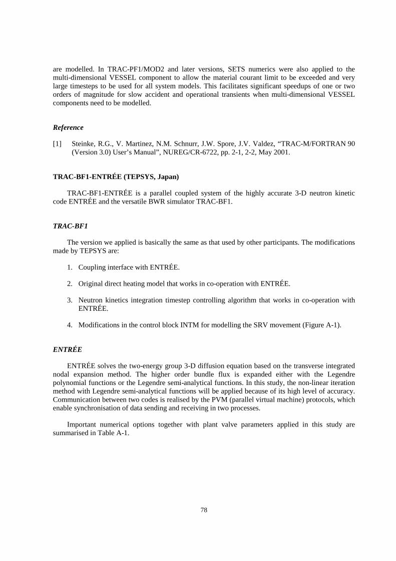
78

are modelled. In TRAC-PF1/MOD2 and later versions, SETS numerics were also applied to themulti-dimensional VESSEL component to allow the material courant limit to be exceeded and verylarge timesteps to be used for all system models. This facilitates significant speedups of one or twoorders of magnitude for slow accident and operational transients when multi-dimensional VESSELcomponents need to be modelled.

Reference

[1] Steinke, R.G., V. Martinez, N.M. Schnurr, J.W. Spore, J.V. Valdez, “TRAC-M/FORTRAN 90(Version 3.0) User’s Manual”, NUREG/CR-6722, pp. 2-1, 2-2, May 2001.

TRAC-BF1-ENTRÉE (TEPSYS, Japan)

TRAC-BF1-ENTRÉE is a parallel coupled system of the highly accurate 3-D neutron kineticcode ENTRÉE and the versatile BWR simulator TRAC-BF1.

TRAC-BF1

The version we applied is basically the same as that used by other participants. The modificationsmade by TEPSYS are:

1. Coupling interface with ENTRÉE.

2. Original direct heating model that works in co-operation with ENTRÉE.

3. Neutron kinetics integration timestep controlling algorithm that works in co-operation withENTRÉE.

4. Modifications in the control block INTM for modelling the SRV movement (Figure A-1).

ENTRÉE

ENTRÉE solves the two-energy group 3-D diffusion equation based on the transverse integratednodal expansion method. The higher order bundle flux is expanded either with the Legendrepolynomial functions or the Legendre semi-analytical functions. In this study, the non-linear iterationmethod with Legendre semi-analytical functions will be applied because of its high level of accuracy.Communication between two codes is realised by the PVM (parallel virtual machine) protocols, whichenable synchronisation of data sending and receiving in two processes.

Important numerical options together with plant valve parameters applied in this study aresummarised in Table A-1.

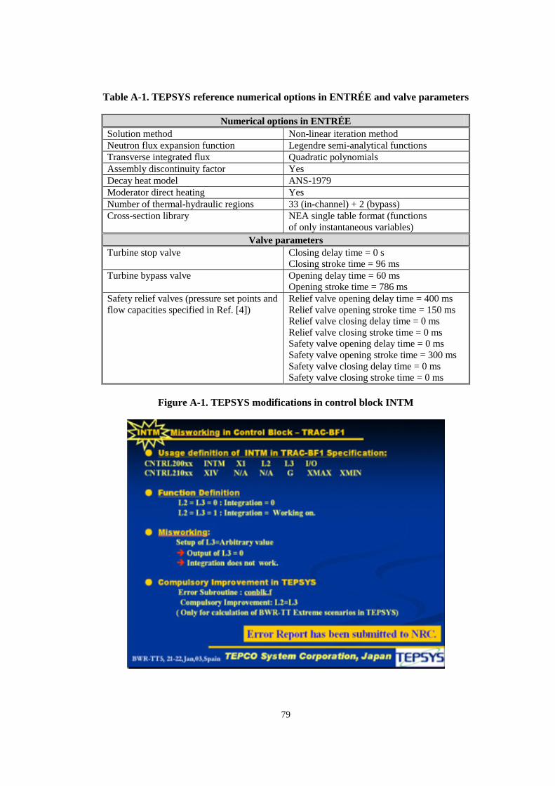
79

Table A-1. TEPSYS reference numerical options in ENTRÉE and valve parameters

Numerical options in ENTRÉESolution method Non-linear iteration methodNeutron flux expansion function Legendre semi-analytical functionsTransverse integrated flux Quadratic polynomialsAssembly discontinuity factor YesDecay heat model ANS-1979Moderator direct heating YesNumber of thermal-hydraulic regions 33 (in-channel) + 2 (bypass)Cross-section library NEA single table format (functions

of only instantaneous variables)Valve parameters

Turbine stop valve Closing delay time = 0 sClosing stroke time = 96 ms

Turbine bypass valve Opening delay time = 60 msOpening stroke time = 786 ms

Safety relief valves (pressure set points andflow capacities specified in Ref. [4])

Relief valve opening delay time = 400 msRelief valve opening stroke time = 150 msRelief valve closing delay time = 0 msRelief valve closing stroke time = 0 msSafety valve opening delay time = 0 msSafety valve opening stroke time = 300 msSafety valve closing delay time = 0 msSafety valve closing stroke time = 0 ms

Figure A-1. TEPSYS modifications in control block INTM

80

RELAP5 (UPISA, Italy)

The light water reactor transient analysis code, RELAP5, was developed at the Idaho NationalEngineering Laboratory for the US Nuclear Regulatory Commission. Code uses include: analysesrequired to support rulemaking, licensing audit calculations, evaluation of accident mitigation strategies,evaluation of operator guidelines and experiment planning analysis. RELAP5 has also been used asthe basis for a nuclear plant analyser. Specific applications have included simulations of transients inLWR systems such as loss-of-coolant, anticipated transients without scram and operational transients(e.g. loss of feedwater, loss of offsite power, station blackout and turbine trip). RELAP5 is a highlygeneric code that, in addition to calculating the behaviour of a reactor coolant system during atransient, can be used for simulation of a wide variety of hydraulic and thermal transients in bothnuclear and non-nuclear systems involving mixtures of steam, water, non-condensables and solutes.

The RELAP5/MOD3 code is based on a non-homogeneous and non-equilibrium model for thetwo-phase system and is solved by a fast, partially implicit numerical scheme to permit economicalcalculation of system transients. The objective from the outset of the RELAP5 development effort wasto produce a code that included important first-order effects necessary for the accurate prediction ofsystem transients but that was also sufficiently simple/cost effective for parametric/sensitivity studies.

The code includes many generic component models from which general systems can be simulated.The component models include pumps, valves, pipes, heat-releasing or absorbing structures, reactorpoint kinetics, electric heaters, jet pumps, turbines, separators, accumulators and control systemcomponents. In addition, special process models are included for effects such as form loss, flow at anabrupt area change, branching, choked flow, boron tracking and non-condensable gas transport.

The system mathematical models are coupled into an efficient code structure. The code includesextensive input checking capability to help the user discover input errors and inconsistencies. Alsoincluded are free-format input, restart, renodalisation and variable output edit features. These userconveniences were developed in recognition that the major cost associated with the use of a systemtransient code is the engineering labour/time involved in accumulating system data and developingsystem models, while the computer cost associated with the generation of final results is usually small.

The development of models and code versions that constitute RELAP5 has spanned ~17 years,from the early stages of the RELAP5 numerical scheme development to the present. RELAP5represents the aggregate accumulation of experience in modelling reactor core behaviour duringaccidents, two-phase flow processes and LWR systems. Code development has benefited fromextensive application and comparison to experimental data in LOFT, PBF, Semiscale, ACRR, NRUand other test programs. The latest version used in the Peach Bottom BWR TT Benchmark isRELAP5/MOD3.3.

TRAC-BF1-VALKIN (UPV, Spain)

The coupled code is called TRAC-BF1-VALKIN and it can be used to simulate transients whileconsidering neutronic phenomena in 3-D geometry and thermal-hydraulic processes in multiplechannel 1-D geometry.

TRAC-BF1

As the thermal-hydraulic code we used the best-estimate code TRAC-BF1, which has a two-fluid,six-equation model to account for the thermal-hydraulic phenomena.

81

To model the heat transfer in the fuel, an axial-radial heat transfer equation is utilised. Thethermal-hydraulics processes are modelled solving six balance equations of mass, momentum and energyfor liquid and vapour phases. For the numerical integration of the fluid flow equations, a semi-implicittwo-step method is used for time discretisation and a first order finite difference method withstaggered mesh is applied to discretise the spatial portion of the equations.

VALKIN

The neutronic code used is the VALKIN module. This module has two options, MODKIN andNOKIN. MODKIN is based on a nodal modal method to integrate the time-dependent neutrondiffusion equation in the approximation of two energy groups. It is also based on the expansion of theneutronic flux in terms of the dominant lambda modes of a given configuration of the reactor core.NOKIN option uses a one-step backward discretisation of the neutron diffusion equation.

NEM

Neutronic code NEM was used to compare the results obtained from the VALKIN code. NEM isa 3-D kinetic code based on the nodal expansion method.

POLCA-T (Westinghouse, Sweden)

POLCA-T is a coupled 3-D core neutron kinetics and system thermal-hydraulics computercode [1]. The code is able to perform steady state and transient analysis of BWR. To varying extents,the code is based on models and tools for BWR and PWR analysis used in the POLCA7 [2], BISONand RIGEL codes [3]. The code utilises new advanced methods and models in neutron kinetics,thermal-hydraulics and numerics. The main features of the code can be summarised as follows:

• Full 3-D model of the reactor core. The neutronic models in the code are the same as those inthe well-known static core analyser POLCA7 with the addition of a proper 3-D kinetics model.

• Advanced five-equation thermal-hydraulic model with a thermal non-equilibrium descriptionof the steam-water mixture and its coupling to the heat structures. Separate mass and energybalances of the phases. Drift flux model that can handle all flow regimes.

• Heat transfer model that also works in post-dryout.

• The gas phase consists of steam and non-condensable gases. The liquid phase containsdissolved non-condensable gas.

• Boron transport model.

• Use of the same thermal-hydraulics model for core and plant systems.

• Two-dimensional fuel rod heat transfer model, gas gap model consistent with design code andcomplete range of heat transfer regimes. The code is able to model all plant heat structures.

• Dryout and DNB correlations (using pin power distributions model).

82

• Full geometrical flexibility of the code: volume cells, flow paths, heat structures, materials,pumps, measurements, controls, etc. are all input data. Code is able to analyse different powerplants and test facilities.

• Balance of plant, control and safety systems: reactor pressure vessel, external pump loops,steam system, feedwater system, ECC systems and steam relief system are modelled todesired detail. A large and valuable set of existent input models can be used.

• Stable numerical method that allows long timesteps, which is also used for a steady statesolution. Low dependence on the size of the timestep since the implicit numerical integrationis close to second order by means of θ-weighting.

Due to the above mentioned features, the POLCA-T code makes possible a comprehensiveapproach to plant analysis with full consistency in steady state and transient calculations. Consistencyin BWR core and system modelling, when transient analyses are performed, is achieved by using thesame basic model and the same design database for core data (cross-section data, burn-up, xenon andother 3-D distributions obtained from depletion calculations), fuel thermal-mechanical behaviour(properties) and system data. Thus, full consistency is also possible between predicted core and systemparameters and their behaviour in a very wide range of phenomena and processes important both fordesign and safety analyses.

Application areas of the POLCA-T code consist of three groups: 1) BWR steady state core design,2) BWR stability, transients and accident analyses and 3) modelling of experimental test facilities.

Applications for BWR steady state core design are covered by POLCA7’s broad capabilities:

• Evaluation of reactivity and power distribution at cold and hot core conditions.

• Detailed thermal-hydraulic analysis.

• Control operations (reactivity search modes including boron, power, flow, control rod, axialoffset and minimum boron control).

• Detector simulation.

• Evaluation of fuel pins, pellet powers and burn-up.

• Evaluation of peaking factors based on pin results.

• Dryout and DNB margin calculations (based on pin power distributions).

• Fission heat load parameters (margins) calculations.

• Pellet cladding interaction calculations.

• Depletion calculation with tracking of most important fissile isotopes and fission products.

• Fuel bundle, control rod, fuel channel and fixed in-core detector depletion.

• Shutdown margin evaluation.

83

• Shutdown cooling.

• Xenon transients.

• Reactivity coefficients (void, burn-up and moderator temperature).

Applications for BWR safety analysis include operational transient, stability, RIA, ATWS,ATWC and LOCA as follows:

• Feedwater flow increase/temperature decrease transients.

• Loss of feedwater flow transients.

• Pressure increase transients – analysis on cladding.

• Pressure increase transients – analysis on the reactor coolant pressure boundary.

• Pressure decrease transients.

• Recirculation flow increase transients.

• Recirculation flow decrease transients.

• Control rod withdrawal error.

• Inadvertent loading transients.

• Control rod drop accident.

• Stability analysis.

• Anticipated transients without scram.

• Anticipated transients without control rods (ATWC).

The POLCA-T code is well-adapted to analyse the type of scenarios with a number of failingcontrol rods. The boron transport model makes it possible to analyse different types of boron shutdownscenarios. Applications for the modelling of separate test facilities (e.g. FRIGG) are foreseen not onlyfor code validation but also for pre-test analysis and experiment planning and optimisation.

References

[1] Panayotov, D., U. Bredolt, P. Jerfsten, “POLCA-T – Consistent BWR Core and SystemsModelling”, ANS/AESJ/ENS Int. Conf. Top Fuel 2003, Paper 410, Wurzburg, Germany,16-19 March 2003.

[2] Lindahl, S-Ö., E. Müller, “Status of ABB Atom’s Core Simulator POLCA”, Int. Conf.PHYSOR96, Mito, Japan, 16-20 September 1996.

84

[3] Wijkström, H., “ABB Atom’s New Code for 3D Static and Transient Analysis”, Proceedings ofthe German Nuclear Society Workshop on Thermal and Fluid Dynamics, Reactor Physics andComputing Methods, Rossendorf, Germany, 31 January through 1 February 2000.

[4] Panayotov, D., “OECD/NRC BWR Turbine Trip Benchmark: Simulation by POLCA-T Code”,PHYSOR2002 International Conference on the New Frontiers of Nuclear Technology: ReactorPhysics, Safety and High-Performance Computing, Track H-2, Paper 3C-02, Seoul, Korea.

85

Appendix B

QUESTIONNAIRE FOR EXERCISE 1 OFTHE NEA-NRC BWR TT BENCHMARK

87

QUESTIONNAIRE FOR EXERCISE 1

1. Thermal-hydraulic model and nodalisation of the vessel and balance of the plant

a) What kind of nodalisation is used (1-D, 3-D and number of T-H channels or cells)?

b) How are the volumes, junctions and channels/T-H cells chosen? (If possible, please provideschematic.)

c) Please provide in detail the nodalisation of the steam line.

2. Boundary conditions

a) Which core thermal-hydraulic initial and transient boundary conditions are used and how?

b) Which neutronic/power initial and transient boundary conditions are used and how?

3. Component design and modelling

a) How many core bypass channels are used in this exercise?

b) How are the jet pumps modelled?

c) How is the steam separator modelled?

d) How are the turbine stop valve closing and steam bypass system modelled?

e) What were the difficulties encountered during the component design modelling?

4. General

a) Deviations from the updated final specifications?

b) User assumptions? Please provide the timestep(s) size or maximum and minimum values usedfor the simulation of Exercise 1.

c) Specific features of the codes used?

d) Number of solutions submitted per participant and how they differ?

e) If your results are significantly different (> 3σ) than the measured or Exelon results, arethere any explanations for these differences? Please explain each significant difference.

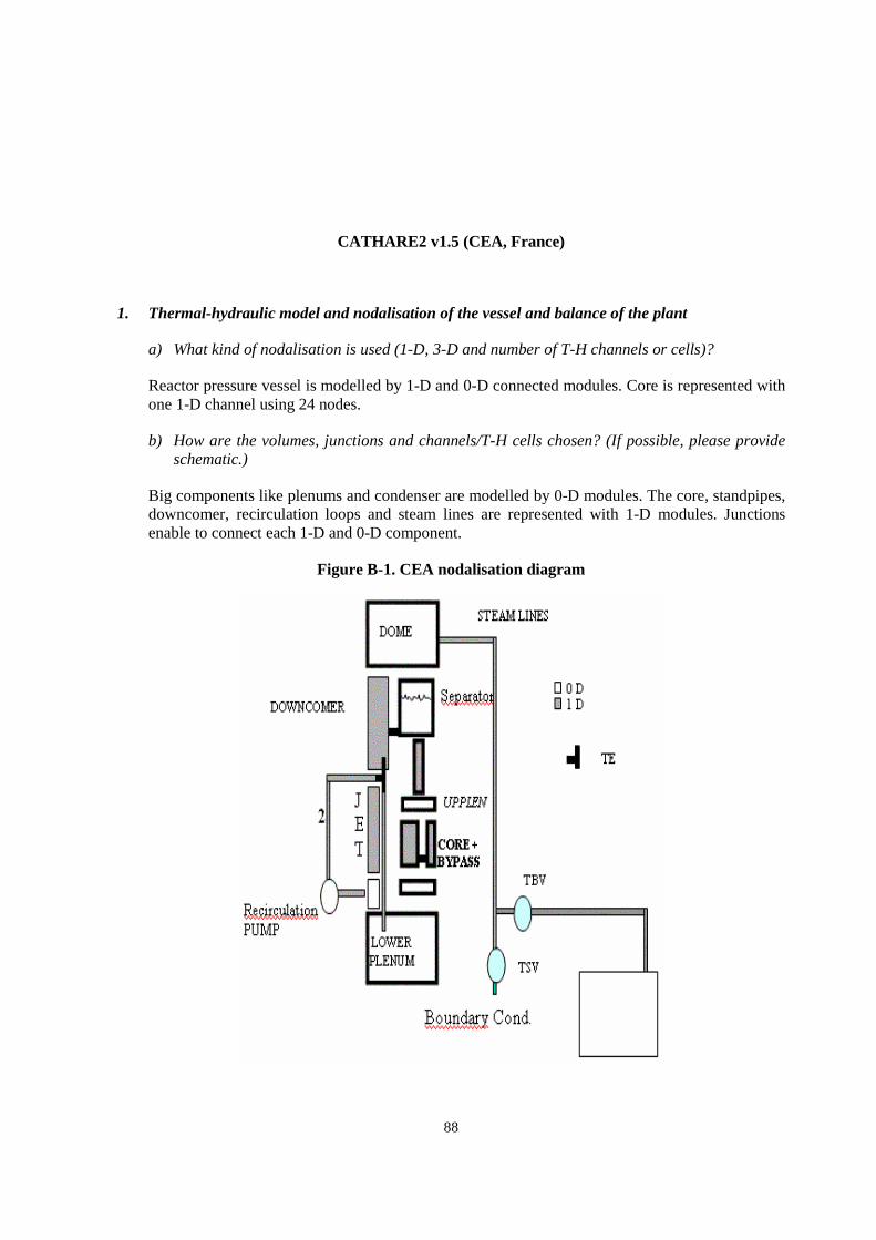
88

CATHARE2 v1.5 (CEA, France)



Reactor pressure vessel is modelled by 1-D and 0-D connected modules. Core is represented withone 1-D channel using 24 nodes.


Big components like plenums and condenser are modelled by 0-D modules. The core, standpipes,downcomer, recirculation loops and steam lines are represented with 1-D modules. Junctionsenable to connect each 1-D and 0-D component.

Figure B-1. CEA nodalisation diagram

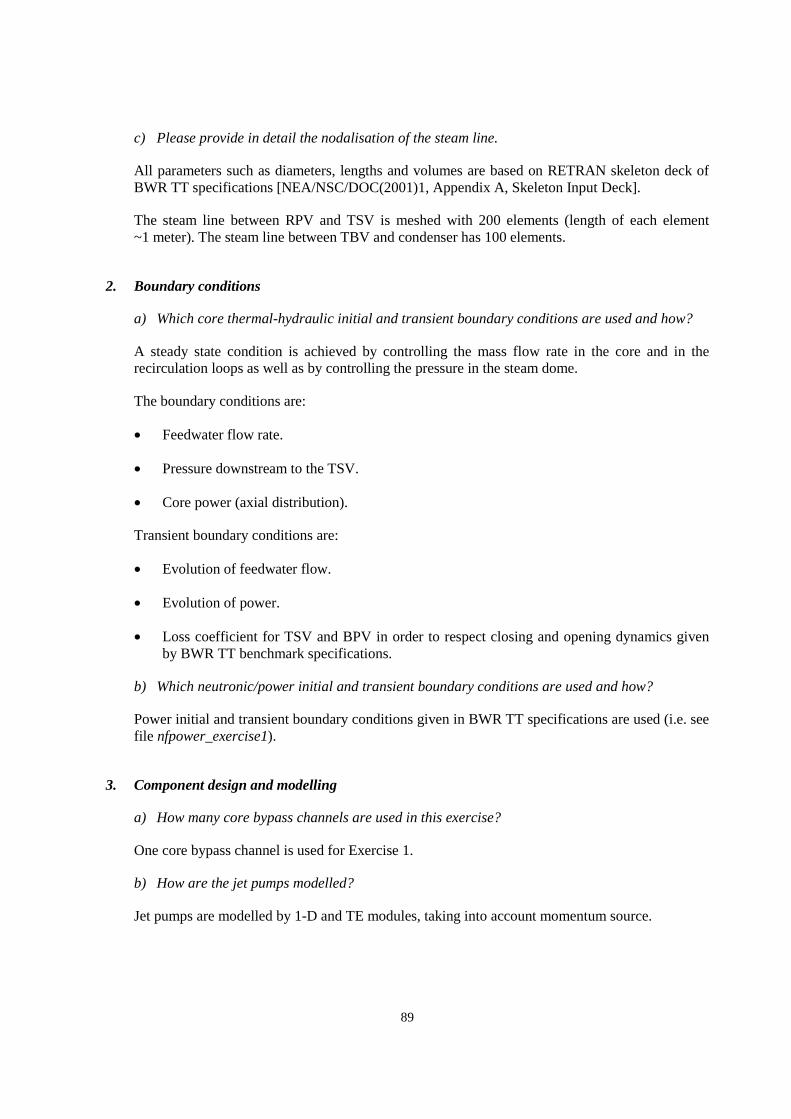
89


All parameters such as diameters, lengths and volumes are based on RETRAN skeleton deck ofBWR TT specifications [NEA/NSC/DOC(2001)1, Appendix A, Skeleton Input Deck].

The steam line between RPV and TSV is meshed with 200 elements (length of each element~1 meter). The steam line between TBV and condenser has 100 elements.



A steady state condition is achieved by controlling the mass flow rate in the core and in therecirculation loops as well as by controlling the pressure in the steam dome.

The boundary conditions are:

• Feedwater flow rate.

• Pressure downstream to the TSV.

• Core power (axial distribution).

Transient boundary conditions are:

• Evolution of feedwater flow.

• Evolution of power.

• Loss coefficient for TSV and BPV in order to respect closing and opening dynamics givenby BWR TT benchmark specifications.


Power initial and transient boundary conditions given in BWR TT specifications are used (i.e. seefile nfpower_exercise1).



One core bypass channel is used for Exercise 1.


Jet pumps are modelled by 1-D and TE modules, taking into account momentum source.

90


The steam separator model utilised is the CATHARE simple separator model with constantcarry-under ratios.


TSV and BPV are modelled by a head-loss coefficient, which is adjusted to simulate the valveclosing and opening.


No particular difficulty was encountered for global modelling.

4. General



The maximum timestep value for the transient calculation is 10–4 s. A sensitivity study showedthat results were not modified if the timestep was kept lower than 0.005 s.


CATHARE is a best-estimate code for LWR transient analysis. The code is based on a six-equation,two-phase flow model with a set of closure laws assessed on a large number of experiments.


One solution for Exercise 1.


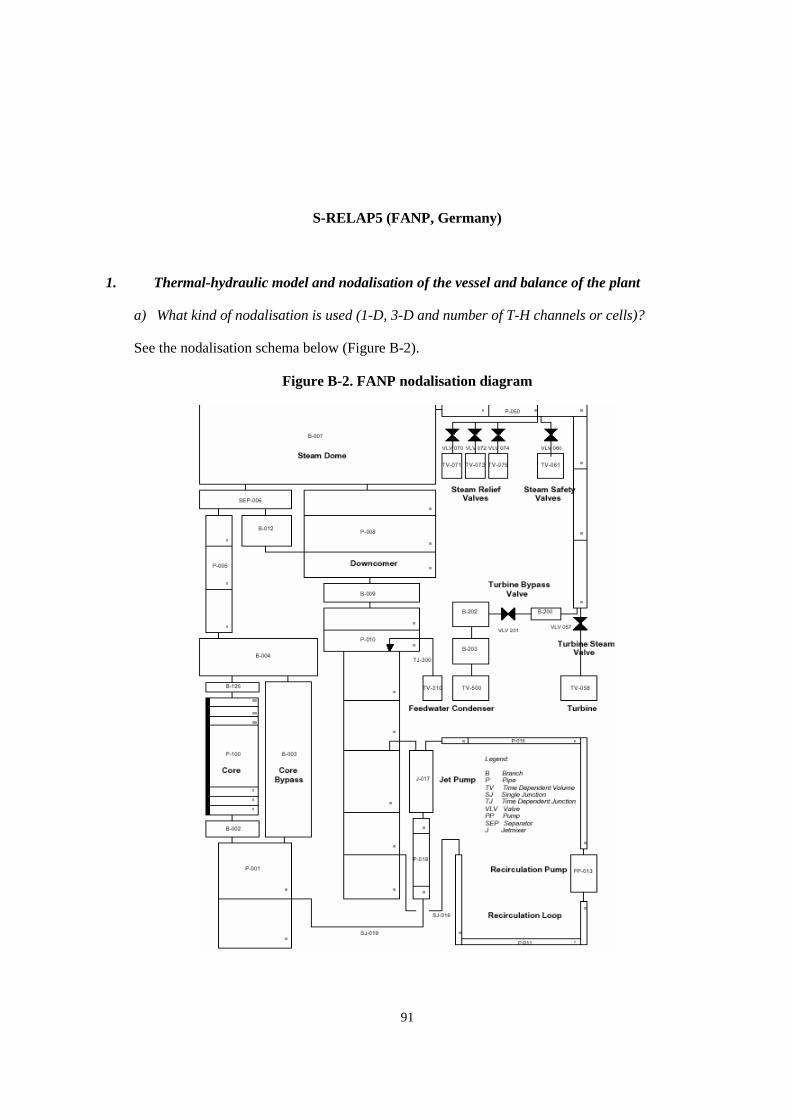
91

S-RELAP5 (FANP, Germany)



See the nodalisation schema below (Figure B-2).

Figure B-2. FANP nodalisation diagram

92


Close to RETRAN nodalisation schema.


See the FANP nodalisation diagram (Figure B-2).



Boundary conditions provided by the benchmark team.


Boundary conditions provided by the benchmark team.



One.


S-RELAP5 standard component.


S-RELAP5 standard component.


Turbine stop valve – linear closure within 96 ms.

Steam bypass system – modelled in such a way that the steam outflow value of RETRAN(provided by the benchmark team) matched the final specifications.


4. General


None.

93


Six milliseconds (6 ms).




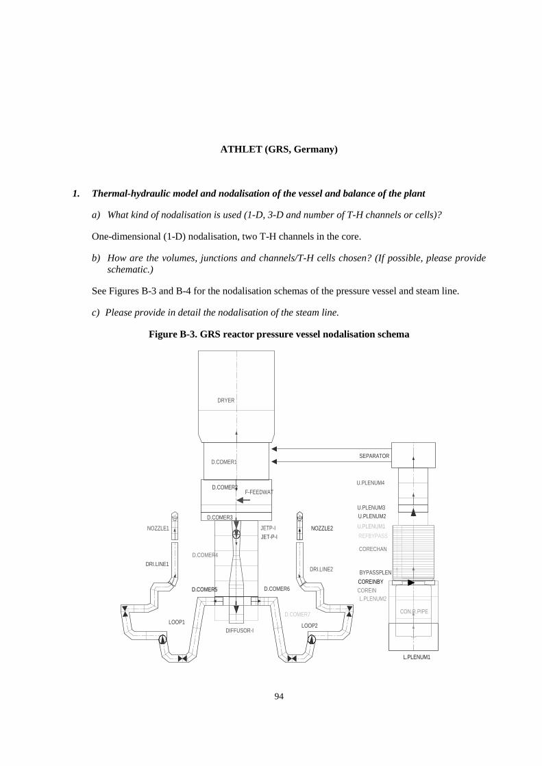
94

ATHLET (GRS, Germany)



One-dimensional (1-D) nodalisation, two T-H channels in the core.


See Figures B-3 and B-4 for the nodalisation schemas of the pressure vessel and steam line.


Figure B-3. GRS reactor pressure vessel nodalisation schema

D.COMER2

D.COMER3

JETP-IJET-P-I

DIFFUSOR-I

L.PLENUM1

L.PLENUM2COREIN

CORECHAN

U.PLENUM1

U.PLENUM2U.PLENUM3

U.PLENUM4

SEPARATORD.COMER1

D.COMER4

D.COMER5

LOOP1

DRI.LINE1

NOZZLE1

LOOP2

DRI.LINE2

NOZZLE2

CON.R.PIPE

BYPASSPLEN

REFBYPASS

COREINBYD.COMER6

D.COMER7

DRYER

F-FEEDWAT

95

Figure B-4. GRS steam line nodalisation schema

DRYER

MSL

BYPLINE

B-TDV

MTV



Mass flow rate at core inlet = 10 580.89 kg/s.

Bypass mass flow rate = 841.8 kg/s.

Pressure at core dome – as measured at steady state.

Core pressure losses adapted to 0.82 bar and mean void to 30.4%.

Core inlet enthalpy – as specified.


Axial power distribution – as specified.

Power history – as specified.

3. Component design


One bypass channel.

96


The model consists of two symmetrical recirculation loops. The mass flow rate through the jetpumps and the pressure difference are adjusted to specifications (see nodalisation schema).


The steam separator is modelled by a corresponding module of ATHLET.

d) How are the turbine stop event and steam bypass flow simulated?

The turbine stop valve closing is modelled by a linear change of the flow area within the closuretime. The steam bypass valve is opened by a linear change of the flow area within the openingtime. It is assumed that critical flow conditions constantly exist and that in fully opened conditionthe mass flow rate is ~600 kg/s.

e) What were the difficulties encountered during the component design?

Great effort was made to approximate the pressure distribution within the reactor vesselcorresponding to the given values from the plant.

4. General


No considerable deviations.



Five-equation model of the thermal-hydraulics.


Only one solution delivered.

f) If your results are significantly different (> 3σ) than the measured or Exelon results, arethere any explanations for these differences? Please explain each significant difference.

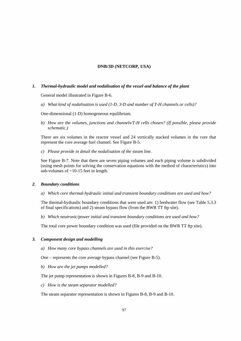
97

DNB/3D (NETCORP, USA)


General model illustrated in Figure B-6.


One-dimensional (1-D) homogeneous equilibrium.


There are six volumes in the reactor vessel and 24 vertically stacked volumes in the core thatrepresent the core average fuel channel. See Figure B-5.


See Figure B-7. Note that there are seven piping volumes and each piping volume is subdivided(using mesh points for solving the conservation equations with the method of characteristics) intosub-volumes of ~10-15 feet in length.



The thermal-hydraulic boundary conditions that were used are: 1) feedwater flow (see Table 5.3.3of final specifications) and 2) steam bypass flow (from the BWR TT ftp site).


The total core power boundary condition was used (file provided on the BWR TT ftp site).



One – represents the core average bypass channel (see Figure B-5).


The jet pump representation is shown in Figures B-8, B-9 and B-10.


The steam separator representation is shown in Figures B-8, B-9 and B-10.

98


The turbine stop valve position closing was assumed to close linearly with time; however, thenon-linear area as a function of position was included in the model. The steam bypass flow wasbased on the boundary condition as noted in Figure B-10.


No difficulties were encountered in the component modelling.

4. General

a) Deviations from the updated final specifications.

There were no known deviations from the final specifications.

b) User assumptions. Please provide the timestep(s) size or maximum and minimum values usedfor the simulation of Exercise 1.

The thermal-hydraulic timestep size was 0.01s for reactor vessel regions and 0.001 s for steamline regions.


See the code description for DNB/3D in Appendix A.


Only one solution was submitted.

e) If your results are significantly different (> 3σ) than the measurement or Exelon results, arethere any explanations for these differences? Please explain each significant difference.

There are no known significant differences.

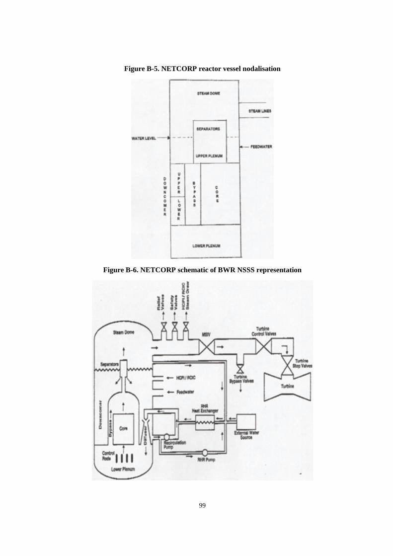
99

Figure B-5. NETCORP reactor vessel nodalisation

Figure B-6. NETCORP schematic of BWR NSSS representation

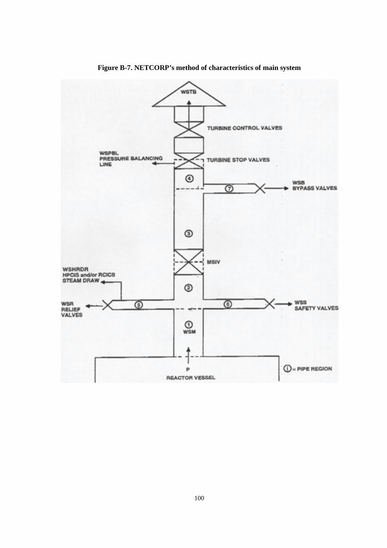
100

Figure B-7. NETCORP’s method of characteristics of main system

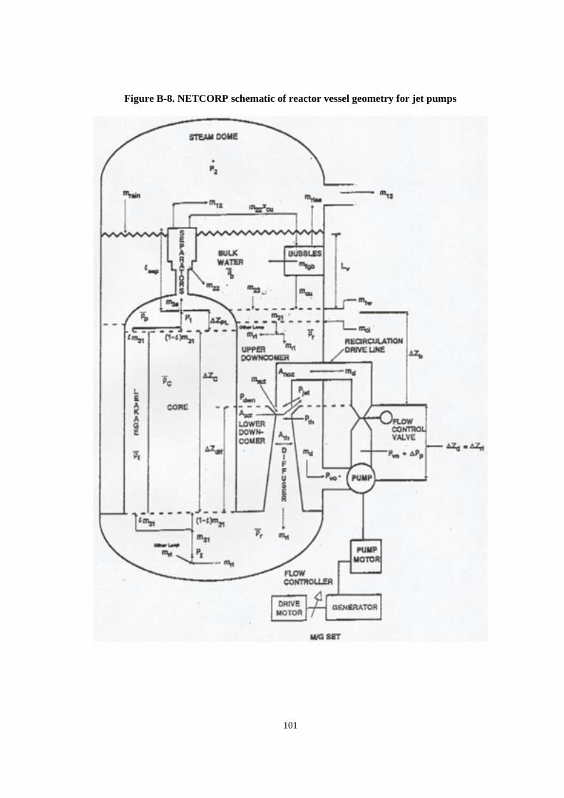
101

Figure B-8. NETCORP schematic of reactor vessel geometry for jet pumps

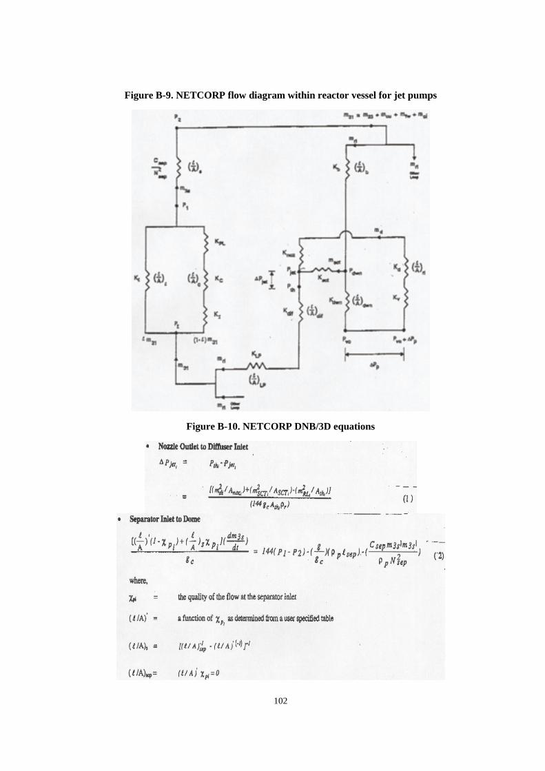
102

Figure B-9. NETCORP flow diagram within reactor vessel for jet pumps

Figure B-10. NETCORP DNB/3D equations

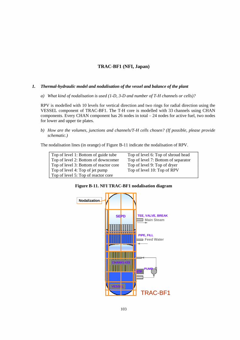
103

TRAC-BF1 (NFI, Japan)



RPV is modelled with 10 levels for vertical direction and two rings for radial direction using theVESSEL component of TRAC-BF1. The T-H core is modelled with 33 channels using CHANcomponents. Every CHAN component has 26 nodes in total – 24 nodes for active fuel, two nodesfor lower and upper tie plates.


The nodalisation lines (in orange) of Figure B-11 indicate the nodalisation of RPV.

Top of level 1: Bottom of guide tube Top of level 6: Top of shroud headTop of level 2: Bottom of downcomer Top of level 7: Bottom of separatorTop of level 3: Bottom of reactor core Top of level 9: Top of dryerTop of level 4: Top of jet pump Top of level 10: Top of RPVTop of level 5: Top of reactor core

Figure B-11. NFI TRAC-BF1 nodalisation diagram

Feed Water

Main Steam

VESSEL

PUMP

PIPE, FILL

TEE, VALVE, BREAK

JETP

NodalizationNodalizationNodalization

TRACTRAC--BF1BF1

SEPD

CHAN#1-#33

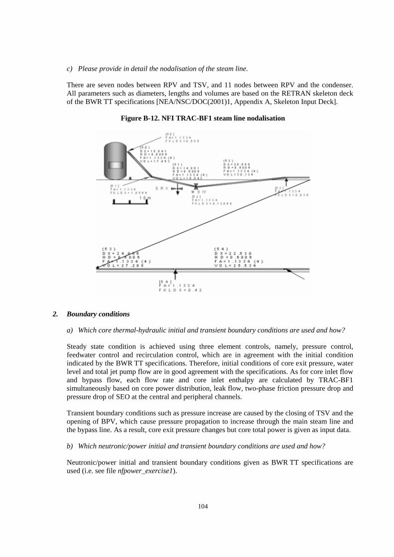
104


There are seven nodes between RPV and TSV, and 11 nodes between RPV and the condenser.All parameters such as diameters, lengths and volumes are based on the RETRAN skeleton deckof the BWR TT specifications [NEA/NSC/DOC(2001)1, Appendix A, Skeleton Input Deck].

Figure B-12. NFI TRAC-BF1 steam line nodalisation



Steady state condition is achieved using three element controls, namely, pressure control,feedwater control and recirculation control, which are in agreement with the initial conditionindicated by the BWR TT specifications. Therefore, initial conditions of core exit pressure, waterlevel and total jet pump flow are in good agreement with the specifications. As for core inlet flowand bypass flow, each flow rate and core inlet enthalpy are calculated by TRAC-BF1simultaneously based on core power distribution, leak flow, two-phase friction pressure drop andpressure drop of SEO at the central and peripheral channels.

Transient boundary conditions such as pressure increase are caused by the closing of TSV and theopening of BPV, which cause pressure propagation to increase through the main steam line andthe bypass line. As a result, core exit pressure changes but core total power is given as input data.


Neutronic/power initial and transient boundary conditions given as BWR TT specifications areused (i.e. see file nfpower_exercise1).

105



Core bypass channels are not used as CHAN but as VESSEL components. Levels 3 and 4 ofVESSEL correspond to the bypass region. We neglect direct heating in core bypass region.


The JETP component is used. The specification is the same as Table 3.1.2.2 and Figure 3.1.2.1 ofthe BWR TT specifications. The junction loss coefficients (jet pump nozzle, suction, etc.) areutilised using the TRAC-BF1 recommended value.


The SEPD component is used. The simple separator model in TRAC-BF1 is selected, so thecarry-under ratio keeps constant during the transient.


The characteristics of Tables 5.2.1 and 5.2.2 of BWR TT benchmark specifications are used forTSV and BPV, respectively.


As for Exercise 1, there is no outstanding difficulty for component design modelling.

4. General



The minimum and maximum timestep value of TRAC-BF1 is 3.0 × 10–5s and 3.0 × 10–1 s,respectively. The actual timestep value is changing between them during the calculation.


TRAC-BF1 is a best-estimate code for BWR transient or accident analysis. This code includesa full non-homogeneous, non-equilibrium, two-fluid thermal-hydraulic model of two-phase flow.


It is our view that the difference between the participants is caused by two main reasons. One isthe difference between codes and their models. The codes would be different in physical modelsversus thermal-hydraulic models. Another is the difference of nodalisation. The modelling ofmain steam lines/RPV or pressure loss profile along pipelines affects pressure propagation/increase.


106

TRAC-BF1 (NUPEC, Japan)



The reactor pressure vessel is modelled in 3-D cylindrical co-ordinates with two radial rings and15 axial levels. Thermal-hydraulic channels were treated as three 1-D parallel channels.


See Figure B-13.


See Figure B-13.

Figure B-13. NUPEC Peach Bottom 2 plant nodalisation

107



Core flow rate and feedwater at initial were from the final specifications. Feedwater flow rate andtemperature during the transient were also from the final specifications.


Fission power was from the final specifications. Decay heat was taken in account.



Core bypass region was simulated by one vessel region. The core bypass flow was simulated witha leak path model from the T-H channel to the vessel (core bypass) region.


The jet pumps were modelled with the JETP component of TRAC-BF1, following Table 3.1.2.2and Figure 3.1.2.1 in the final specifications.


The steam separators were modelled with SEPD component using a mechanistic model ofTRAC-BF1. Code defaults were used.


The turbine stop valve and steam bypass valve were modelled with the VALVE component ofTRAC-BF1. The valve movements were given as timetables.


Simulation of inertia of the steam separators.

4. General


None.


Timesteps: 0.5-1.0 ms.


None.

108


One.


Our result was within 3σ of the measured result.

NUPEC used the TRAC-BF1 code in the first exercise. Peach Bottom 2 plant nodalisation isshown above in Figure B-13. The thermal-hydraulic channels were treated as three 1-D parallelchannels. The reactor pressure vessel is modelled in 3-D cylindrical co-ordinates with two radialrings and 15 axial levels.

109

RETRAN-3D (PSI, Switzerland)



A 1-D nodalisation with 53 volumes and 63 junctions is used. The core region between the lowerplenum and the upper plenum is represented by a core inlet volume, a core exit volume, a corebypass volume and a T-H channel representing the core, which consists of 24 axially stackedvolumes with pre-defined power.


For the modelling of the transient, we used the code RETRAN-3D. Although the referencesolution for the benchmark was developed using RETRAN-02 [by Andy Olson (Exelon/USA)] inorder to fit the results as much as possible, we decided to develop a PSI RETRAN-3D model. Theaim was to increase our team’s learning curve. Our RETRAN-3D input model for the phase 1calculation was developed from an early RETRAN-02 model for Turbine Trip 1 [Hornyik andNaser, 1979]. From this model, we used the nodalisation for the reactor vessel (including thesteam separator and downcomer region), the recirculation loop and the steam lines. Aspreparation for the inclusion of the 3-D core in the later benchmark phases, the reactor coreregion was renodalised (including the accompanying heat structures) to include 24 axial controlvolumes, in combination with a core exit volume and core inlet volume connected to the corebypass volume. From the benchmark specifications, we included the time-dependence and axialprofile of the pre-defined power, together with the feedwater flow, the turbine inlet flow rate andthe turbine bypass area of Turbine Trip 2. In addition, the value of enthalpy in the lower plenum,steam dome pressure and flow rates at t = 0 were used.

We investigated the sensitivity of our model with respect to non-equilibrium effects in the steamseparator region and to pressure losses in the turbine bypass line. The improvements with respectto the non-equilibrium effects were included in the 3-D model, since they influence the magnitudeand timing of the power maximum. Improvements relating to pressure losses in the turbine bypassline (effective only after t = 2 s) were not included.

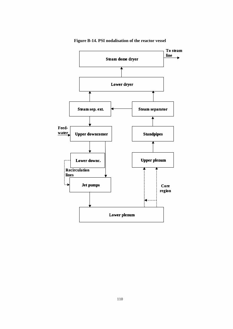
110

Figure B-14. PSI nodalisation of the reactor vessel

Lower downc.

Jet pumps

Upper downcomer

Steam sep. ext.

Upper plenum

Standpipes

Steam separator

Lower dryer

Lower plenum

To steamline

Recirculationlines

Coreregion

Steam dome dryer

Feed-water

Lower downc.Lower downc.

Jet pumpsJet pumps

Upper downcomerUpper downcomer

Steam sep. ext.Steam sep. ext.

Upper plenumUpper plenum

StandpipesStandpipes

Steam separatorSteam separator

Lower dryerLower dryer

Lower plenumLower plenum

To steamline

Recirculationlines

Coreregion

Steam dome dryerSteam dome dryer

Feed-water

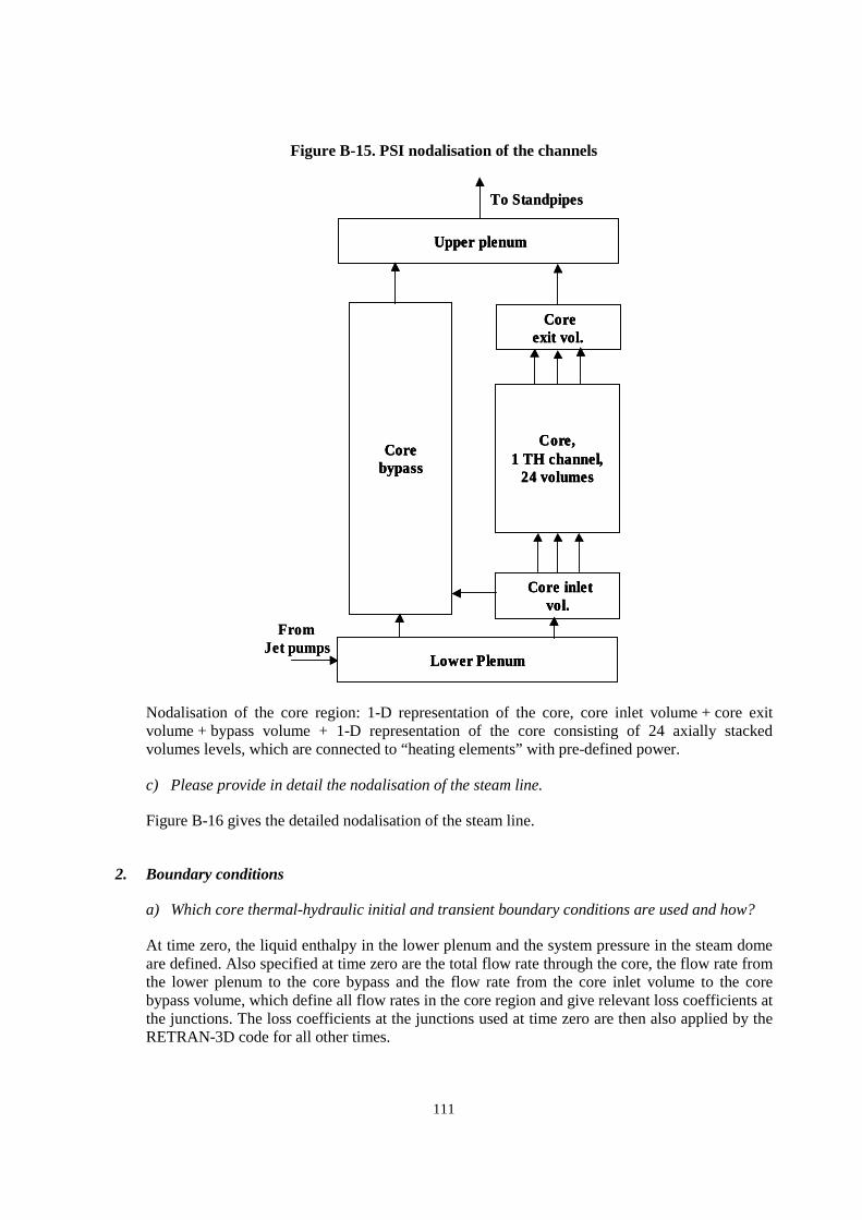
111

Figure B-15. PSI nodalisation of the channels

Core inletvol.

Upper plenum

Lower Plenum

FromJet pumps

Coreexit vol.

Corebypass

Core,1 TH channel,

24 volumes

To Standpipes

Core inletvol.

Core inletvol.

Upper plenumUpper plenum

Lower PlenumLower Plenum

FromJet pumps

Coreexit vol.

Coreexit vol.

CorebypassCore

bypass

Core,1 TH channel,

24 volumes

Core,1 TH channel,

24 volumes

To Standpipes

Nodalisation of the core region: 1-D representation of the core, core inlet volume + core exitvolume + bypass volume + 1-D representation of the core consisting of 24 axially stackedvolumes levels, which are connected to “heating elements” with pre-defined power.


Figure B-16 gives the detailed nodalisation of the steam line.



At time zero, the liquid enthalpy in the lower plenum and the system pressure in the steam domeare defined. Also specified at time zero are the total flow rate through the core, the flow rate fromthe lower plenum to the core bypass and the flow rate from the core inlet volume to the corebypass volume, which define all flow rates in the core region and give relevant loss coefficients atthe junctions. The loss coefficients at the junctions used at time zero are then also applied by theRETRAN-3D code for all other times.

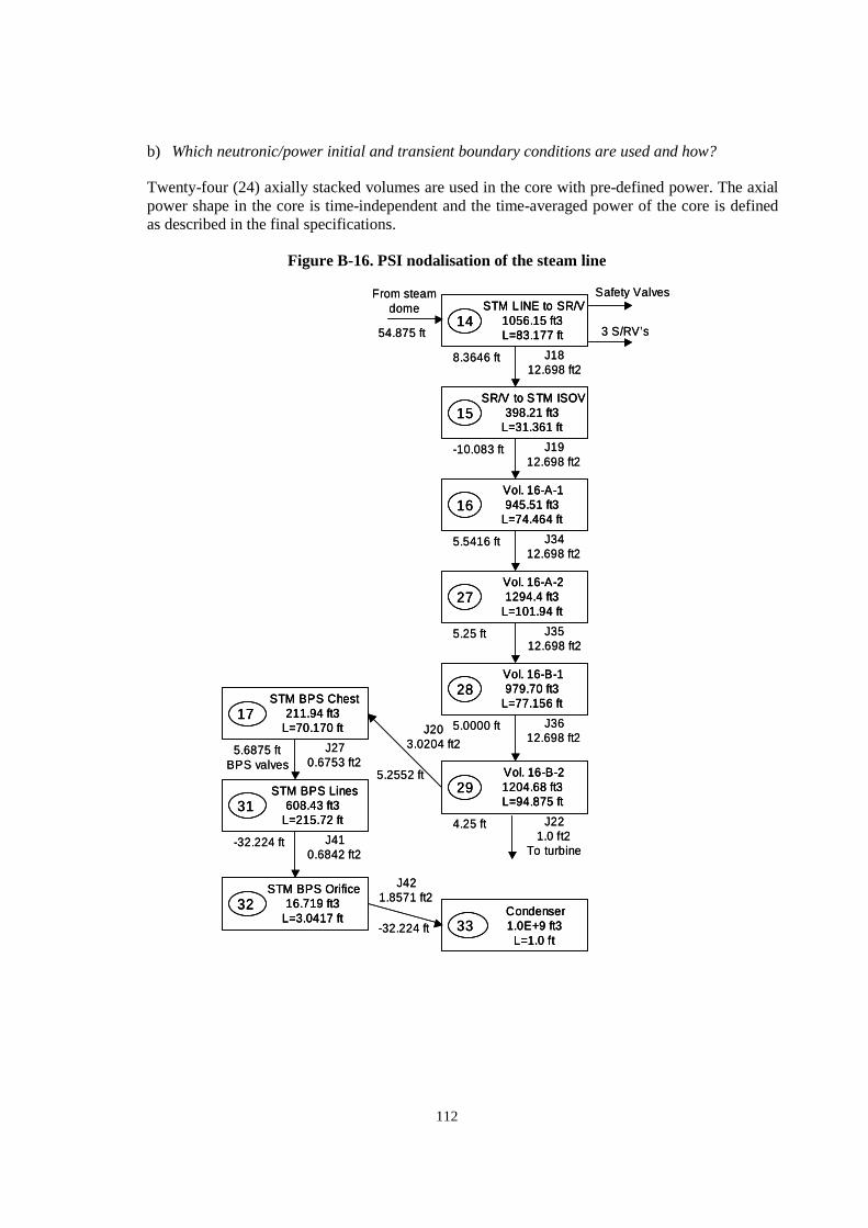
112


Twenty-four (24) axially stacked volumes are used in the core with pre-defined power. The axialpower shape in the core is time-independent and the time-averaged power of the core is definedas described in the final specifications.

Figure B-16. PSI nodalisation of the steam line

From steamdome

54.875 ft

SR/V to STM ISOV398.21 ft3

L=31.361 ft15

J1912.698 ft2

-10.083 ft

Vol. 16-A-1945.51 ft3

L=74.464 ft16

J3412.698 ft2

5.5416 ft

Vol. 16-A-21294.4 ft3

L=101.94 ft27

J3512.698 ft2

5.25 ft

Vol. 16-B-1979.70 ft3

L=77.156 ft28

J3612.698 ft2

5.0000 ft

STM LINE to SR/V1056.15 ft3L=83.177 ft

14

J1812.698 ft2

8.3646 ft

Vol. 16-B-21204.68 ft3L=94.875 ft

29

J221.0 ft2

To turbine

4.25 ft

STM BPS Chest211.94 ft3

L=70.170 ft17

J270.6753 ft2

5.6875 ftBPS valves

STM BPS Lines608.43 ft3

L=215.72 ft31

J410.6842 ft2

-32.224 ft

STM BPS Orifice16.719 ft3

L=3.0417 ft32

J421.8571 ft2

-32.224 ftCondenser1.0E+9 ft3

L=1.0 ft33

Safety Valves

3 S/RV’s

J203.0204 ft2

5.2552 ft

From steamdome

54.875 ft


L=31.361 ft15


L=31.361 ft15

J1912.698 ft2

-10.083 ft

Vol. 16-A-1945.51 ft3

L=74.464 ft16

Vol. 16-A-1945.51 ft3

L=74.464 ft16

J3412.698 ft2

5.5416 ft

Vol. 16-A-21294.4 ft3

L=101.94 ft27

Vol. 16-A-21294.4 ft3

L=101.94 ft27

J3512.698 ft2

5.25 ft

Vol. 16-B-1979.70 ft3

L=77.156 ft28

Vol. 16-B-1979.70 ft3

L=77.156 ft28

J3612.698 ft2

5.0000 ft

STM LINE to SR/V1056.15 ft3L=83.177 ft

14STM LINE to SR/V

1056.15 ft3L=83.177 ft

14

J1812.698 ft2

8.3646 ft

Vol. 16-B-21204.68 ft3L=94.875 ft

29Vol. 16-B-21204.68 ft3L=94.875 ft

29

J221.0 ft2

To turbine

4.25 ft


L=70.170 ft17


L=70.170 ft17

J270.6753 ft2

5.6875 ftBPS valves


L=215.72 ft31


L=215.72 ft31

J410.6842 ft2

-32.224 ft


L=3.0417 ft32


L=3.0417 ft32

J421.8571 ft2

-32.224 ftCondenser1.0E+9 ft3

L=1.0 ft33

Condenser1.0E+9 ft3

L=1.0 ft33

Safety Valves

3 S/RV’s

J203.0204 ft2

5.2552 ft

113



One core bypass channel.


The jet pumps are modelled using a RETRAN-3D pump model.


In order to determine the distribution of the steam flow, it is important to follow the flow of steamthrough the separators into the steam dome. In the reactor, two-phase flow from the core regionpasses through the standpipes and then enters the steam separators. In each separator, thesteam-water mixture passes turning vanes, which impart a spin to establish a vortex and separatesthe water from the steam. The denser liquid is thrown radially outward by centrifugal forceforming a continuous film on the inside wall of the inner pipe. The separator water exits fromunder the separator cap and flows out between the standpipes, draining into the downcomer.Steam with a quality of at least 90% exits from the top of the separator and rises to the dryers.The dryers force the wet steam to be directed horizontally through the dryer panels. The steamflow makes a series of rapid changes in direction while traversing the panels. During thesedirection changes, the heavier drops of entrained moisture are forced to the outer walls wheremoisture collection hooks catch and drain the liquid to collection troughs, then through tubes intothe vessel downcomer so that the steam dryer assembly increases the quality of the steam to morethan 99.9%. This dry steam flows into the steam dome and the steam lines.

This behaviour is approximated in the RETRAN-3D model by control volumes (CV 1-5 inFigure B-17). Two-phase flow from the core region flows into the steam separator volume (CV 1).In this volume, a liquid level is defined, below which a two-phase flow is established. Above theliquid level there is only steam flow. In this volume (CV 1), the RETRAN-3D bubble rise modeloption is used. The steam flows upwards to the lower dryer volume (CV 2) and continues to thesteam dome volume (CV 3) and into the steam line.

Two-phase flow, which consists of water with some vapour carry-under, flows from the steamseparator volume to the steam separator external volume (CV 4). The junction between these twocontrol volumes is below the liquid level in CV 1. In the steam separator external (CV 4), a liquidlevel develops with a steam phase above the liquid level and a two-phase region below the liquidlevel. The RETRAN-3D bubble rise model is again used to describe this phenomenon. At t = 0there is a very small steam flow from the steam separator external to the lower dryer volume(CV 2), while the main flow is water down into the upper downcomer (CV 5). The feedwater alsoflows into the upper downcomer volume. From the upper downcomer volume, water flows to thelower downcomer and jet pumps, and from there back into the core.

Since the RETRAN-3D code option used in analysis is that of the four-equation model (i.e. fullthermal equilibrium), the volume of water in steam separator (CV 1) and steam separator external(CV 4) two-phase control volumes is in equilibrium with the steam. And, this strongly influencesthe pressure increase per unit of steam generated in the core. As a result, a renodalisation of theseparator/downcomer region was performed in a sensitivity study, which gave a pressure increaseequal to the measured one at ~1 s. In order to achieve this, the volumes of the steam separator andthe steam separator external control volumes were reduced in the sensitivity test, while thevolume of the upper downcomer control volume was increased to preserve the total water volume.

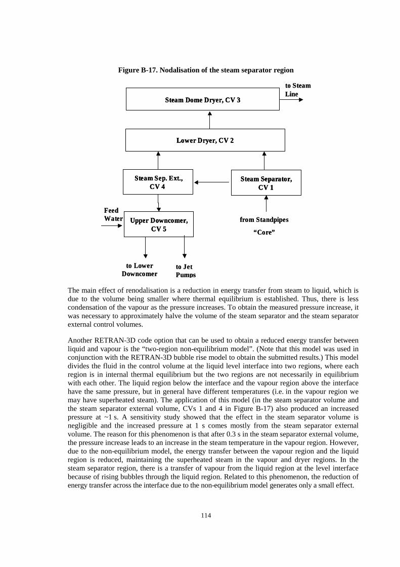
114

Figure B-17. Nodalisation of the steam separator region

Upper Downcomer,CV 5

Steam Sep. Ext.,CV 4

Steam Separator,CV 1

FeedWater

to LowerDowncomer

from Standpipes

“Core”

to JetPumps

to SteamLine

Lower Dryer, CV 2

Steam Dome Dryer, CV 3







FeedWater

to LowerDowncomer

from Standpipes

“Core”

to JetPumps

to SteamLine

Lower Dryer, CV 2Lower Dryer, CV 2

Steam Dome Dryer, CV 3Steam Dome Dryer, CV 3

The main effect of renodalisation is a reduction in energy transfer from steam to liquid, which isdue to the volume being smaller where thermal equilibrium is established. Thus, there is lesscondensation of the vapour as the pressure increases. To obtain the measured pressure increase, itwas necessary to approximately halve the volume of the steam separator and the steam separatorexternal control volumes.

Another RETRAN-3D code option that can be used to obtain a reduced energy transfer betweenliquid and vapour is the “two-region non-equilibrium model”. (Note that this model was used inconjunction with the RETRAN-3D bubble rise model to obtain the submitted results.) This modeldivides the fluid in the control volume at the liquid level interface into two regions, where eachregion is in internal thermal equilibrium but the two regions are not necessarily in equilibriumwith each other. The liquid region below the interface and the vapour region above the interfacehave the same pressure, but in general have different temperatures (i.e. in the vapour region wemay have superheated steam). The application of this model (in the steam separator volume andthe steam separator external volume, CVs 1 and 4 in Figure B-17) also produced an increasedpressure at ~1 s. A sensitivity study showed that the effect in the steam separator volume isnegligible and the increased pressure at 1 s comes mostly from the steam separator externalvolume. The reason for this phenomenon is that after 0.3 s in the steam separator external volume,the pressure increase leads to an increase in the steam temperature in the vapour region. However,due to the non-equilibrium model, the energy transfer between the vapour region and the liquidregion is reduced, maintaining the superheated steam in the vapour and dryer regions. In thesteam separator region, there is a transfer of vapour from the liquid region at the level interfacebecause of rising bubbles through the liquid region. Related to this phenomenon, the reduction ofenergy transfer across the interface due to the non-equilibrium model generates only a small effect.

115


The turbine stop valve closing is described by a negative fill junction model, which is combinedwith a valve where area versus time is specified. This defines the flow rate to the turbine.

The steam bypass system is modelled using four RETRAN-3D control volumes. The steambypass chest volume is connected via the bypass valves to the steam bypass lines volume, whichis connected to the steam bypass orifice volume that is in turn connected to the condenser. In theturbine bypass valve between the steam bypass chest volume and the steam bypass lines volume,area versus time is defined (approximately) to get the specified flow through the turbine bypass.Choked flow through the bypass valve is assumed.


4. General


Since we decided that there would be no point just copying the reference RETRAN-02 model, ourPSI RETRAN-3D model must have some differences in the final specifications [see also responseto question 1b)]. For instance, the nodalisation of steam line, reactor vessel and steam separatorregion is based on the original model from Hornyik and Naser (1979). This means, for example,that the steam separator volume is connected to the steam separator external volume. That is tosay that the two RETRAN-3D volumes with a liquid level are connected, which is not the case inthe Olson model.


The minimum timestep size between 0-1.2 s is 0.001 s and 0.006 s after 1.2 s. However, asensitivity study showed that the effect of choosing an overall minimum timestep of 0.006 swould have only a negligible effect on the results.


As described above, the four-equation model was used for the two-phase flow calculation, togetherwith an algebraic (Zolotar-Lellouche) slip correlation. The bubble rise model was used in the steamseparator and steam separator external volumes to describe the development of a liquid level. Thetwo-region non-equilibrium model was also used in the steam separator and steam separatorexternal volumes to account for the relatively slow exchange of energy across the liquid level.


One solution from PSI.


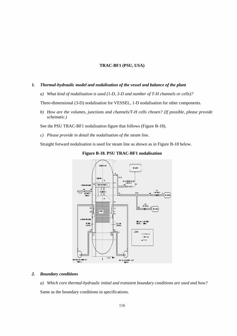
116

TRAC-BF1 (PSU, USA)



Three-dimensional (3-D) nodalisation for VESSEL, 1-D nodalisation for other components.


See the PSU TRAC-BF1 nodalisation figure that follows (Figure B-18).


Straight forward nodalisation is used for steam line as shown as in Figure B-18 below.

Figure B-18. PSU TRAC-BF1 nodalisation



Same as the boundary conditions in specifications.

117


Power lookup table from specifications is used.



No bypass channel is used. Core bypass flow is simulated by leak paths from first cell of channelsto related elevation of the vessel.


Standard jet pump option of TRAC-B is used. See Figure B-18.


Simple separator is used.


Same as specifications.


No difficulties were encountered.

4. General



The convergence criterion is 0.0001 and courant number is 0.999. The timestep size is 6 ms.Some loss coefficients are assumed.


See the TRAC-BF1 code description in Appendix A.


One solution is provided.


The results agree well with the provided reference results.

118

TRAC-M (PSU/NRC, USA)



Three-dimensional (3-D) nodalisation for VESSEL, 1-D nodalisation for other components.


See Figure B-19.


Straight forward nodalisation is used for steam line as shown as in Figure B-19.



Same as the boundary conditions in specifications.


Power lookup table from specifications is used.



No bypass channel is used.


Standard jet pump option of TRAC-M is used. See Figures B-19 and B-20.


Three-stage mechanistic separators are used.

d) How were the turbine stop valve closing and steam bypass system modelled?

They are the same as specifications.

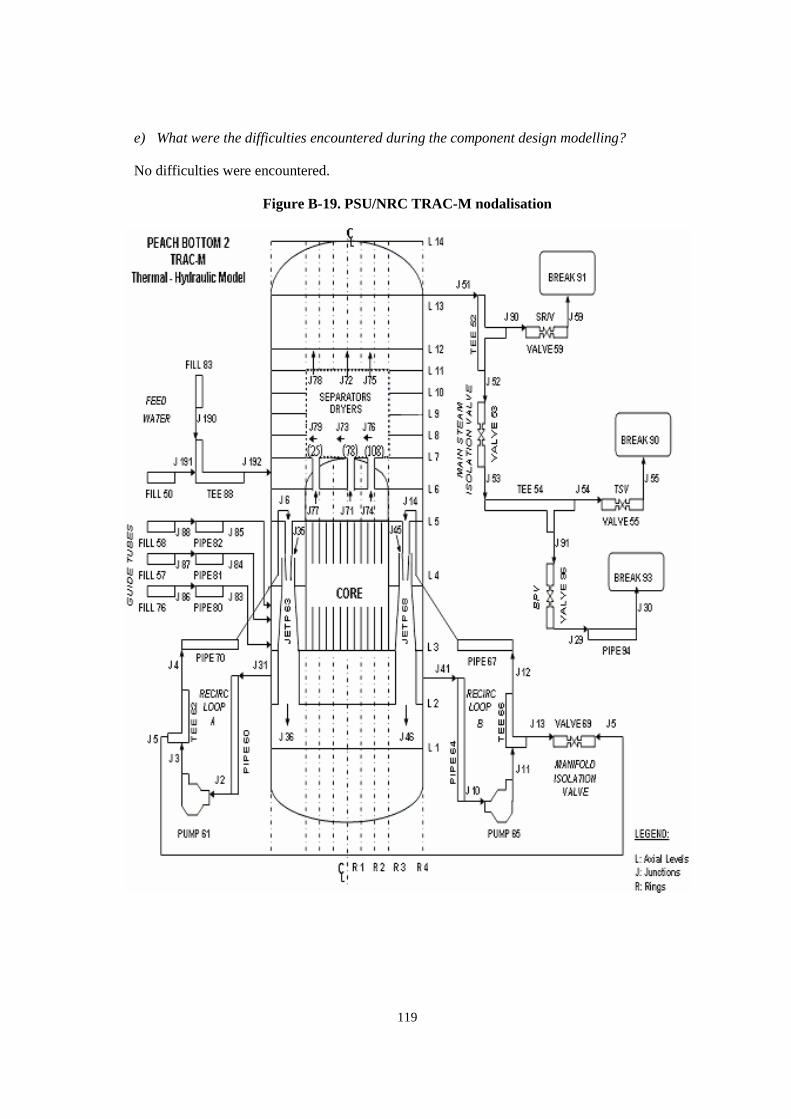
119


No difficulties were encountered.

Figure B-19. PSU/NRC TRAC-M nodalisation

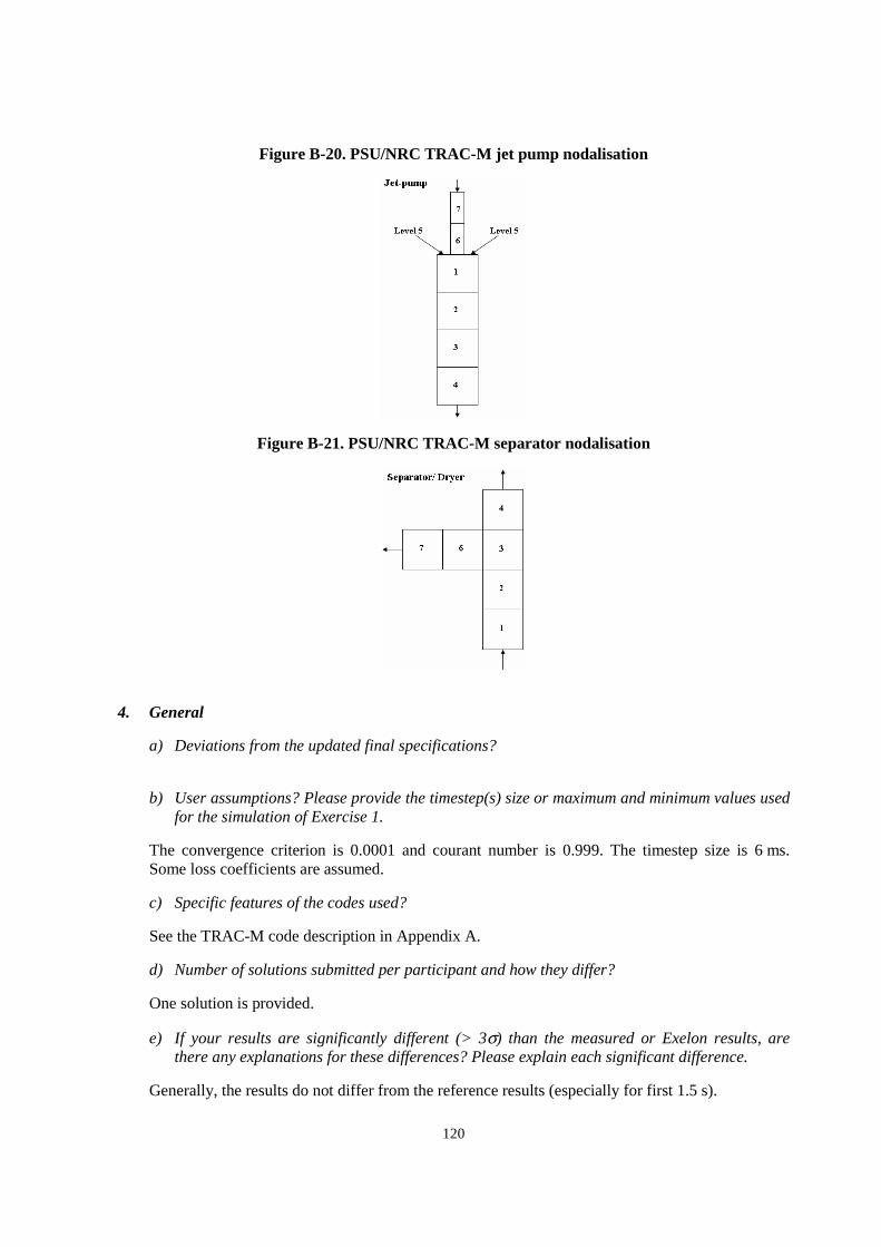
120

Figure B-20. PSU/NRC TRAC-M jet pump nodalisation

Figure B-21. PSU/NRC TRAC-M separator nodalisation

4. General



The convergence criterion is 0.0001 and courant number is 0.999. The timestep size is 6 ms.Some loss coefficients are assumed.


See the TRAC-M code description in Appendix A.


One solution is provided.


Generally, the results do not differ from the reference results (especially for first 1.5 s).

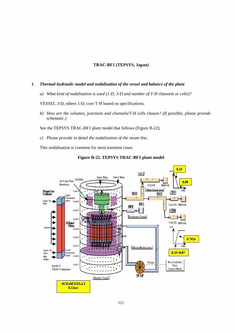
121

TRAC-BF1 (TEPSYS, Japan)



VESSEL 3-D, others 1-D, core T-H based on specifications.


See the TEPSYS TRAC-BF1 plant model that follows (Figure B-22).


This nodalisation is common for most transient cases.

Figure B-22. TEPSYS TRAC-BF1 plant model

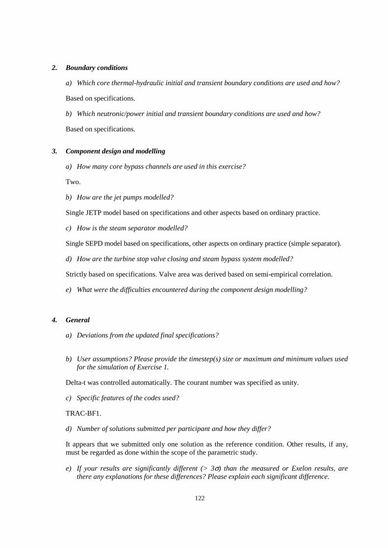
122



Based on specifications.


Based on specifications.



Two.


Single JETP model based on specifications and other aspects based on ordinary practice.


Single SEPD model based on specifications, other aspects on ordinary practice (simple separator).


Strictly based on specifications. Valve area was derived based on semi-empirical correlation.


4. General



Delta-t was controlled automatically. The courant number was specified as unity.


TRAC-BF1.


It appears that we submitted only one solution as the reference condition. Other results, if any,must be regarded as done within the scope of the parametric study.


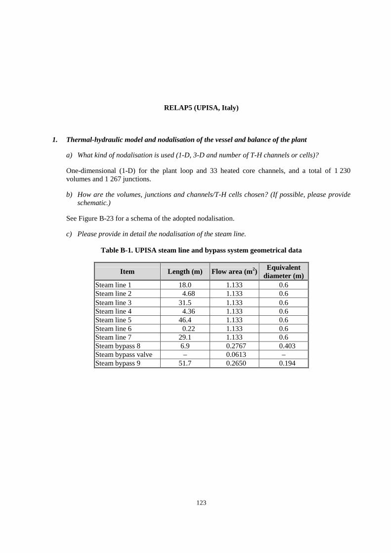
123

RELAP5 (UPISA, Italy)



One-dimensional (1-D) for the plant loop and 33 heated core channels, and a total of 1 230volumes and 1 267 junctions.


See Figure B-23 for a schema of the adopted nodalisation.


Table B-1. UPISA steam line and bypass system geometrical data

Item Length (m) Flow area (m2) Equivalentdiameter (m)

Steam line 1 18.0 1.133 0.6Steam line 2 114.68 1.133 0.6Steam line 3 31.5 1.133 0.6Steam line 4 114.36 1.133 0.6Steam line 5 46.4 1.133 0.6Steam line 6 110.22 1.133 0.6Steam line 7 29.1 1.133 0.6Steam bypass 8 6.9 10.2767 110.403Steam bypass valve – 10.0613 –Steam bypass 9 51.7 10.2650 110.194

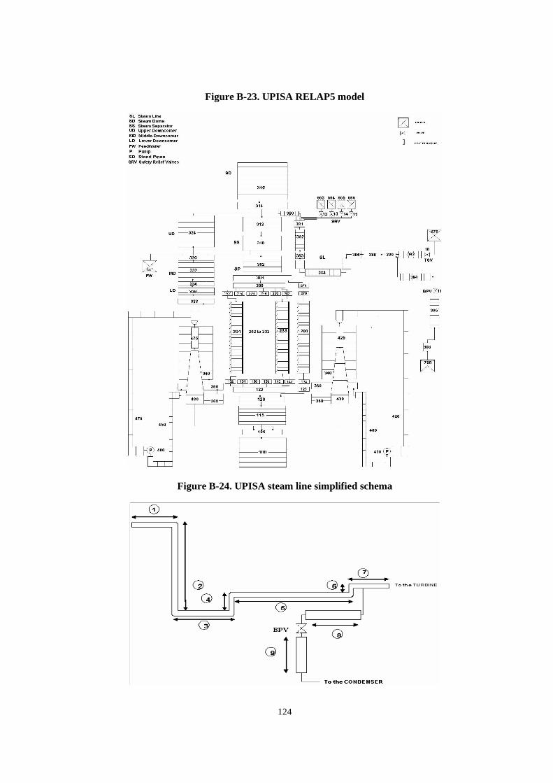
124

Figure B-23. UPISA RELAP5 model

Figure B-24. UPISA steam line simplified schema

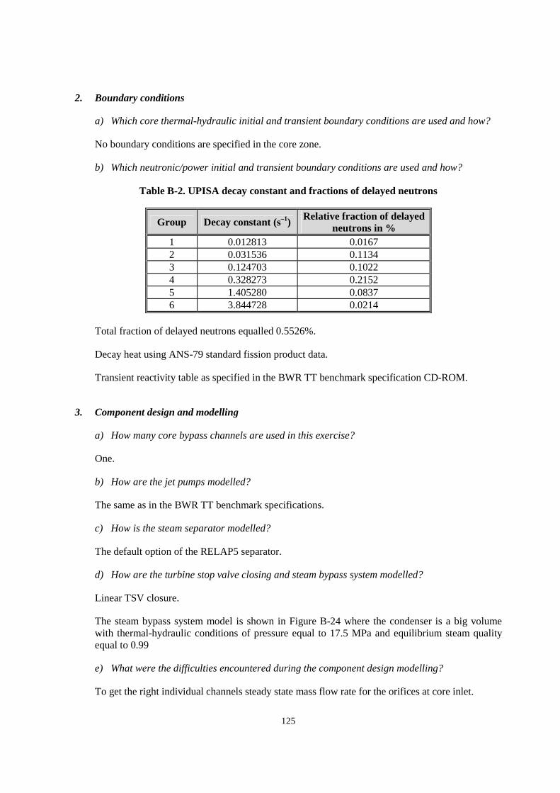
125



No boundary conditions are specified in the core zone.


Table B-2. UPISA decay constant and fractions of delayed neutrons

Group Decay constant (s–1) Relative fraction of delayedneutrons in %

1 0.012813 0.01672 0.031536 0.11343 0.124703 0.10224 0.328273 0.21525 1.405280 0.08376 3.844728 0.0214

Total fraction of delayed neutrons equalled 0.5526%.

Decay heat using ANS-79 standard fission product data.

Transient reactivity table as specified in the BWR TT benchmark specification CD-ROM.



One.


The same as in the BWR TT benchmark specifications.


The default option of the RELAP5 separator.


Linear TSV closure.

The steam bypass system model is shown in Figure B-24 where the condenser is a big volumewith thermal-hydraulic conditions of pressure equal to 17.5 MPa and equilibrium steam qualityequal to 0.99


To get the right individual channels steady state mass flow rate for the orifices at core inlet.

126

4. General



Minimum DT = 1.0 e – 6 s

Maximum DT = 1.0 e – 3 s


The RELAP5/MOD3 code is based on a six-equation non-homogeneous and non-equilibriummodel for the two-phase system. The solutions are obtained through fast resolution of a partiallyimplicit numerical scheme.


Two solutions, the main differences between them are outlined in the table below.

Number ofheated channels

Core pressuredrop MPa Inlet enthalpy

First solution 1 0.0670 1 194.0Second solution 33 0.1025 1 208.5


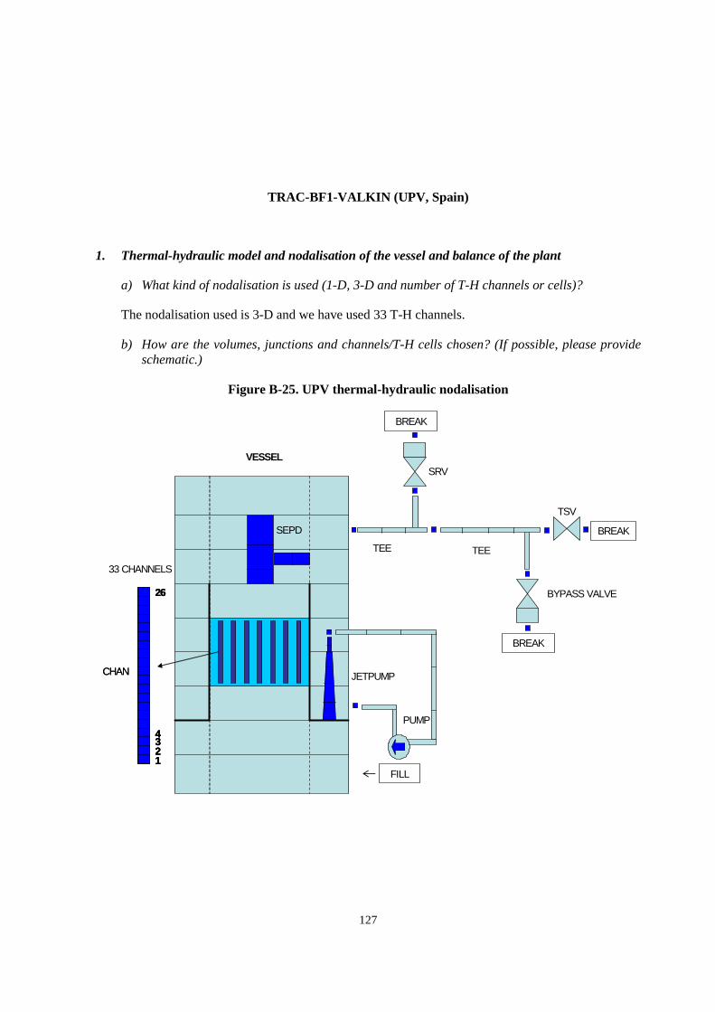
127

TRAC-BF1-VALKIN (UPV, Spain)



The nodalisation used is 3-D and we have used 33 T-H channels.


Figure B-25. UPV thermal-hydraulic nodalisation

TEE

TSV

BYPASS VALVE

BREAK

BREAK

BREAK

TEE

PUMP

VESSEL

SEPD

JETPUMP

33 CHANNELS

CHAN

1234

26

CHAN

1234

26

1234

26

SRV

FILL

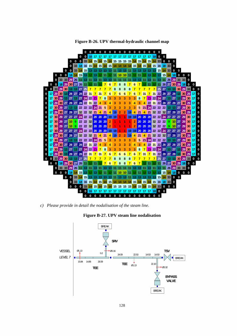
128

Figure B-26. UPV thermal-hydraulic channel map

0 0 0 0 0 0 0 0 0 0 0 0 0 0 0 00 0 18 17 17 17 17 17 17 17 17 17 17 17 17 18 0 0

0 0 0 33 14 15 14 15 14 15 15 15 15 14 15 14 15 14 33 0 0 00 33 18 16 15 14 15 14 15 14 14 14 14 15 14 15 14 15 16 18 33 0

0 0 33 14 15 13 13 13 13 13 11 13 13 11 13 13 13 13 13 15 14 33 0 00 0 0 18 14 15 13 12 13 12 11 12 11 10 10 11 12 11 12 13 12 13 15 14 18 0 0 00 33 33 29 26 11 13 11 13 11 13 13 11 11 11 11 13 13 11 13 11 13 11 26 29 33 33 0

0 0 18 29 30 27 26 11 12 11 12 7 6 7 8 8 7 6 7 12 11 12 11 26 27 30 29 18 0 00 0 33 29 30 13 13 27 25 7 7 7 7 7 8 8 8 8 7 7 7 7 7 25 27 13 13 30 29 33 0 00 17 29 30 13 28 27 28 22 31 7 31 7 6 7 6 6 7 6 7 31 7 31 22 28 27 28 13 30 29 17 00 17 30 29 13 27 13 27 24 22 23 7 8 3 3 3 3 3 3 8 7 23 22 24 27 13 27 13 29 30 17 00 17 29 30 27 28 27 28 22 31 22 4 3 4 3 3 3 3 4 3 4 22 31 22 28 27 28 27 30 29 17 00 17 30 29 27 13 13 22 22 22 24 21 5 3 3 3 3 3 3 5 21 24 22 22 22 13 13 27 29 30 17 00 17 29 30 27 28 27 32 22 32 21 4 21 4 19 2 2 19 4 21 4 21 32 22 32 27 28 27 30 29 17 00 17 30 29 27 27 27 24 22 22 20 20 20 19 19 1 1 19 19 20 20 20 22 22 24 27 27 27 29 30 17 00 17 30 29 27 10 9 22 22 32 20 20 20 2 1 1 1 1 2 20 20 20 32 22 22 9 10 27 29 30 17 00 17 30 29 27 10 9 22 22 32 20 20 20 2 1 1 1 1 2 20 20 20 32 22 22 9 10 27 29 30 17 00 17 30 29 27 27 27 24 22 22 20 20 20 19 19 1 1 19 19 20 20 20 22 22 24 27 27 27 29 30 17 00 17 29 30 27 28 27 32 22 32 21 4 21 4 19 2 2 19 4 21 4 21 32 22 32 27 28 27 30 29 17 00 17 30 29 27 13 13 22 22 22 24 21 5 3 3 3 3 3 3 5 21 24 22 22 22 13 13 27 29 30 17 00 17 29 30 27 28 27 28 22 31 22 4 3 4 3 3 3 3 4 3 4 22 31 22 28 27 28 27 30 29 17 00 17 30 29 13 27 13 27 24 22 23 7 8 3 3 3 3 3 3 8 7 23 22 24 27 13 27 13 29 30 17 00 17 29 30 13 28 27 28 22 31 7 31 7 6 7 6 6 7 6 7 31 7 31 22 28 27 28 13 30 29 17 00 0 33 29 30 13 13 27 25 7 7 7 7 7 8 8 8 8 7 7 7 7 7 25 27 13 13 30 29 33 0 0

0 0 18 29 30 27 26 11 12 11 12 7 6 7 8 8 7 6 7 12 11 12 11 26 27 30 29 18 0 00 33 33 29 26 11 13 11 13 11 13 13 11 11 11 11 13 13 11 13 11 13 11 26 29 33 33 00 0 0 18 14 15 13 12 13 12 11 12 11 10 10 11 12 11 12 13 12 13 15 14 18 0 0 0

0 0 33 14 15 13 13 13 13 13 11 13 13 11 13 13 13 13 13 15 14 33 0 00 33 18 16 15 14 15 14 15 14 14 14 14 15 14 15 14 15 16 18 33 00 0 0 33 14 15 14 15 14 15 15 15 15 14 15 14 15 14 33 0 0 0

0 0 18 17 17 17 17 17 17 17 17 17 17 17 17 18 0 00 0 0 0 0 0 0 0 0 0 0 0 0 0 0 0


Figure B-27. UPV steam line nodalisation

TEE

TSV

BYPASSVALVE

BREAK

BREAK

BREAK

TEE

SRV

VESSEL

LEVEL715.84 14.86 26.59

0.2 24.09 22.53 14.53 14.53

22.10

Ø1.13

Ø1.13

Ø0.16

Ø0.32

129



We used the boundary conditions from specifications.


The initial power was 2 030 MW, and the boundary conditions were from specifications.



We did not use any bypass channels.


The jet pumps are modelled with the jet pump component of TRAC-BF1. The primary tube hasfour cells and secondary one has two cells.


The steam separator was modelled with the TRAC-BF1 component SEPD.


The turbine valve closes at 0.096 s; it is specified in table provided by specifications on valvecomponents.

The steam bypass system is modelled using the data from specifications.


4. General



Timestep size of 0.1 s.



We submitted one solution.


130

POLCA-T (Westinghouse, Sweden)



Three-dimensional (3-D) nodalisation with 764 T-H channels, 24 fuel nodes and two nodes forthe bottom and top reflector in each channel.


One T-H channel per fuel assembly, 122 radial reflector channels.


Main steam lines are modelled by steam lines, safety and relieve valves, turbine stop valves andsteam head with a total of 65 nodes and five valves.



Power versus timetable, turbine pressure controller set point versus time, bypass valve positionversus time and feedwater mass flow.


See response to question 2a).



One.


The POLCA-T jet pumps model is used, which is validated against full and 1/6 scale test facilitydata and has nodalisation similar to that used in TRAC-M calculations.


The POLCA-T steam separator model is used, which is validated against our test data.

131


The turbine stop valve closing is modelled by a signal-activated turbine pressure controller. Thecontroller’s set point versus timetable is given as a boundary condition.

Bypass valve position versus time is given as a boundary condition. The steam bypass systemmodel covers: bypass chest, bypass valves, lines and orifice, and steam condenser with a total of51 nodes and one valve.

d) What were the difficulties encountered during the component design modelling?

There were no difficulties encountered during the component design modelling. However, to setup the plant model there was the need for a sensitivity study on some of the parameters [such ascarry-under and carry-over, turbine stop valve closing (linear or non-linear model), and jet pumpmodel to work along the M-N curve].

4. General


We did not see any.


Constant timestep as given in the specifications (0.006 s).


Core description given in the input data of our neutronics code POLCA-7, POLCA-T steamseparator model, POLCA-T jet pumps model, control rods speed and position controller, scramcontroller, jet pump drive flow controller, feedwater controller, RPV water level controller andturbine pressure controller.


One solution.


OECD PUBLICATIONS, 2 rue André-Pascal, 75775 PARIS CEDEX 16 Printed in France.

Documents

BOILING WATER REACTOR TURBINE TRIP (TT) BENCHMARK€¦ · · 2005-08-12BOILING WATER REACTOR TURBINE TRIP (TT) ... sponsorship a PWR main steam line break (MSLB) benchmark against