Statistics & Probability Letters 52 (2001) 73–78

Bounds for optimal stopping values of dependentrandom variables with given marginals

Alfred M�uller ∗

Institut f�ur Wirtschaftstheorie und Operations Research, Universit�at Karlsruhe, Geb. 20.21, Kaiserstrasse 12,D-76128 Karlsruhe, Germany

Received October 1999; received in revised form February 2000

Abstract

We consider the problem of optimal stopping of a �nite sequence of dependent random variables. We explicitly determinethe maximum of the stopping value within the Fr�echet class of all multivariate distributions with given continuousmarginals. We show that the maximum is attained for a shu�e of min copula, and that it coincides with the value of aprophet. c© 2001 Elsevier Science B.V. All rights reserved

Keywords: Optimal stopping; Bounds; Distributions with given marginals; Copula; Prophet inequalities

1. Introduction

For a �nite sequence X = (X1; : : : ; Xn) of n random variables, we de�ne the optimal stopping value V (X)as

V (X) := sup�∈T

EX�;

where T is the set of all stopping times for (X1; : : : ; Xn). According to Chow et al. (1971), V (X) can bedetermined, in principle, by a backward induction method. If the sequence (X1; : : : ; Xn) is independent or atleast Markovian, then this leads to an easy computation, but it is practically infeasible, if we allow arbitrarydependencies between the components. In that case, it is interesting to �nd bounds for V (X). Rinott andSamuel-Cahn (1987,1991) have shown that a weak condition of negative dependence leads to an increase ofthe optimal stopping value compared with the case of independent components.In this paper, we try to �nd bounds for V (X) under the condition that we know the marginal distributions

F1; : : : ; Fn, but that we do not know the dependence structure. Formally, let � = �(F1; : : : ; Fn) be the set of

∗ Tel.: +49-721-608-4737; fax: +49-721-608-6057.E-mail address: mueller@wior.uni-karlsruhe.de (A. M�uller).

0167-7152/01/$ - see front matter c© 2001 Elsevier Science B.V. All rights reservedPII: S0167 -7152(00)00220 -0

74 A. M�uller / Statistics & Probability Letters 52 (2001) 73–78

all n-dimensional distributions with �xed marginals F1; : : : ; Fn. In the literature on statistical dependence thisset is usually called a Fr�echet class, see e.g. Joe (1997). We will try to derive the values of

V+(F1; : : : ; Fn) := maxX∈�(F1 ;:::; Fn)

V (X) and V−(F1; : : : ; Fn) := minX∈�(F1 ;:::; Fn)

V (X):

Our main result will be the explicit solution of the maximum problem for arbitrary continuous F1; : : : ; Fn.The minimum problem seems to be more di�cult. However, we can show that the trivial lower bound EX1is sharp in many important cases.

2. The upper bound

First, we will introduce the stopping rule, and the dependence structure that will lead to the maximum of theproblem maxX∈�V (X). We assume that all distributions F1; : : : ; Fn are continuous. Hence there exists some�∗ ∈ R with ∑n

i=1 1−Fi(�∗)=1. Moreover, we de�ne �∗i := 1−Fi(�∗). Now, we construct the random vectorX̃ with marginals F1; : : : ; Fn as follows. Let U ∼ U (0; 1) be a uniformly distributed real random variable, andde�ne U1 :=U , and recursively Ui+1 :=Ui ⊕ �∗i , i = 1; : : : ; n− 1. Here ⊕ denotes addition modulo 1, i.e.

x ⊕ y :={x + y if x + y6 1;

x + y − 1 if x + y¿ 1:

Now let X̃ i :=F−1i (Ui); i=1; : : : ; n, where as usual F−1

i (z)= inf{t ∈ R : F(t)¿ z} is the generalized inverseof Fi.Notice that the random variables Ui; i=1; : : : ; n are all uniformly distributed, and that the Xi’s are monotone

transformations of the Ui’s. Hence, the dependence structure of X̃ can be described by the distribution Cof U = (U1; : : : ; Un), which is the copula of X̃ . The copula C that we use here, can be considered as amultivariate extension of the well-known shu�es of Min introduced by Mikusinski et al. (1992). Especially,it exhibits complete dependence.As optimal stopping rule we simply use the threshold stopping rule with �∗ as threshold, i.e. �∗ := inf{i :

X̃ i ¿�∗}. In the following theorem, we will show that this stopping rule yields a return that stochasticallydominates the return for any other strategy and any other dependence structure. As usual, we write X 6st Y , ifY stochastically dominates X , i.e. if P(X ¿ t)6P(Y ¿ t) for all t ∈ R. We refer to Shaked and Shanthikumar(1994) for more details about stochastic ordering.

Theorem 2.1. If all distributions F1; : : : ; Fn are continuous; then

X�6st X̃ �∗

for all � ∈ T and all X ∈ �(F1; : : : ; Fn).

Proof. We have de�ned U1; : : : ; Un such that they are all uniformly distributed, and such that for all 16 i¡ j6 nwe have

[Ui ¿ 1− �∗i ] = [0¡Ui+1¡�∗i ] = : : :=

[ j−1∑k=i+1

�∗k ¡Uj ¡j−1∑k=i

�∗k

]:

A. M�uller / Statistics & Probability Letters 52 (2001) 73–78 75

Since∑n

k=1 �∗k =1, we have 1−�∗j ¿

∑j−1k=i �

∗k , and therefore the events [Ui ¿ 1−�∗i ]= [F−1

i (Ui)¿F−1i (1−

�∗i )] = [X̃ i ¿�∗]; i = 1; : : : ; n are disjoint, and form a partition of the probability space. Hence,

P(X̃ �∗ ¿t) =n∑i=1

P(X̃ �∗ ¿t; �∗ = i)

=n∑i=1

P(X̃ i ¿ t; X̃ i ¿�∗)

=min

{1;

n∑i=1

P(X̃ i ¿ t)

}for all t ∈ R:

On the other hand, we have for all � ∈ T and all X ∈ �(F1; : : : ; Fn)

P(X�¿ t) =n∑i=1

P(X�¿ t; �= i)

6n∑i=1

P(Xi ¿ t)

=n∑i=1

P(X̃ i ¿ t)

and hence P(X�¿ t)6min{1;∑ni=1 P(X̃ i ¿ t)}.

Remark. Notice that the distribution of X̃ is singular, since all components X̃ i; i=1; : : : ; n are a deterministicfunction of U . Indeed, all components X̃ i; i=2; : : : ; n can be written as a deterministic function of X1, so thatall uncertainty disappears after observing the �rst variable. Moreover, notice that the components of X̃ exhibitsome sort of negative dependence, since large values never go together. This is, however, an unusual and veryweak sort of negative dependence. Let us assume e.g. that F1 = : : :=Fn=U (0; 1). Then Var(

∑X̃ i)=Var(X̃ 1)

and hence∑

i 6=j Corr(X̃ i; X̃ j) =−(n− 1). Thus, there must be some negative correlation. On the other hand,we have for all i = 1; : : : ; n− 1

Corr(X̃ i; X̃ i+1) = 2(n− 1)3 + 1

n3− 1 → 1 for n→ ∞:

Indeed, if n is very large, then X̃ i and X̃ i+1 are nearly identical. So nearby components are strongly positivelycorrelated, but the components far from each other (e.g. X̃ 1 and X̃ n=2) are negatively correlated.Using the well-known identity EX =

∫∞0 P(X ¿x) dx we can immediately derive the following explicit

expression for V+(F1; : : : ; Fn).

Corollary 2.2. If all distributions F1; : : : ; Fn are continuous; then

V+(F1; : : : ; Fn) = EX̃ �∗ = �∗ +∫ ∞

�∗

(n∑i=1

(1− Fi(t)))dt:

Notice that Theorem 2.1 implies a much more general result than Corollary 2.2. In Corollary 2.2, weconsider the optimal stopping problem for a decision maker who maximizes the expected value, i.e. she is

76 A. M�uller / Statistics & Probability Letters 52 (2001) 73–78

risk neutral. Theorem 2.1 implies, however, that the same result holds also for any decision maker with a(non-decreasing) von Neumann–Morgenstern utility u : R→ R, who faces the decision problem

Vu(X) := sup�∈T

Eu(X�):

For the explicit solution of this problem in the case of independent components we refer to M�uller (2000)and the references therein. Now, de�ne

V+u (F1; : : : ; Fn) := maxX∈�(F1 ;:::; Fn)

Vu(X):

Then, it follows immediately from Theorem 2.1 that

V+u (F1; : : : ; Fn) = Eu(X̃ �∗);

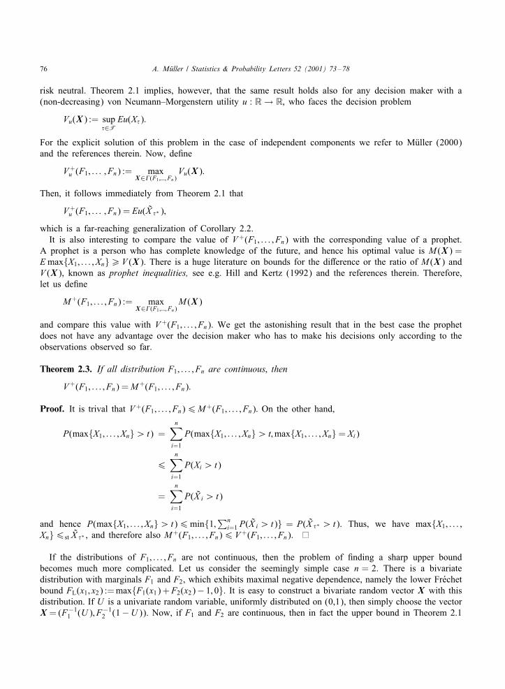
which is a far-reaching generalization of Corollary 2.2.It is also interesting to compare the value of V+(F1; : : : ; Fn) with the corresponding value of a prophet.

A prophet is a person who has complete knowledge of the future, and hence his optimal value is M (X) =Emax{X1; : : : ; Xn}¿V (X). There is a huge literature on bounds for the di�erence or the ratio of M (X) andV (X), known as prophet inequalities, see e.g. Hill and Kertz (1992) and the references therein. Therefore,let us de�ne

M+(F1; : : : ; Fn) := maxX∈�(F1 ;:::; Fn)

M (X)

and compare this value with V+(F1; : : : ; Fn). We get the astonishing result that in the best case the prophetdoes not have any advantage over the decision maker who has to make his decisions only according to theobservations observed so far.

Theorem 2.3. If all distribution F1; : : : ; Fn are continuous; then

V+(F1; : : : ; Fn) =M+(F1; : : : ; Fn):

Proof. It is trival that V+(F1; : : : ; Fn)6M+(F1; : : : ; Fn): On the other hand,

P(max{X1; : : : ; Xn}¿t) =n∑i=1

P(max{X1; : : : ; Xn}¿t;max{X1; : : : ; Xn}= Xi)

6n∑i=1

P(Xi ¿ t)

=n∑i=1

P(X̃ i ¿ t)

and hence P(max{X1; : : : ; Xn}¿t)6min{1;∑ni=1 P(X̃ i ¿ t)} = P(X̃ �∗ ¿t). Thus, we have max{X1; : : : ;

Xn}6st X̃ �∗ , and therefore also M+(F1; : : : ; Fn)6V+(F1; : : : ; Fn).

If the distributions of F1; : : : ; Fn are not continuous, then the problem of �nding a sharp upper boundbecomes much more complicated. Let us consider the seemingly simple case n = 2. There is a bivariatedistribution with marginals F1 and F2, which exhibits maximal negative dependence, namely the lower Fr�echetbound FL(x1; x2) :=max{F1(x1)+F2(x2)− 1; 0}. It is easy to construct a bivariate random vector X with thisdistribution. If U is a univariate random variable, uniformly distributed on (0,1), then simply choose the vectorX = (F−1

1 (U ); F−12 (1−U )). Now, if F1 and F2 are continuous, then in fact the upper bound in Theorem 2.1

A. M�uller / Statistics & Probability Letters 52 (2001) 73–78 77

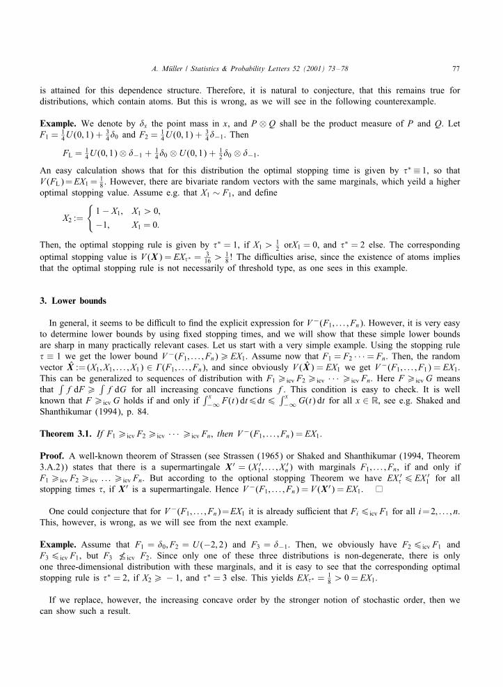
is attained for this dependence structure. Therefore, it is natural to conjecture, that this remains true fordistributions, which contain atoms. But this is wrong, as we will see in the following counterexample.

Example. We denote by �x the point mass in x, and P ⊗ Q shall be the product measure of P and Q. LetF1 = 1

4U (0; 1) +34�0 and F2 =

14U (0; 1) +

34�−1. Then

FL = 14U (0; 1)⊗ �−1 + 1

4�0 ⊗ U (0; 1) + 12�0 ⊗ �−1:

An easy calculation shows that for this distribution the optimal stopping time is given by �∗ ≡ 1, so thatV (FL)=EX1 = 1

8 . However, there are bivariate random vectors with the same marginals, which yeild a higheroptimal stopping value. Assume e.g. that X1 ∼ F1, and de�ne

X2 :=

{1− X1; X1¿ 0;

−1; X1 = 0:

Then, the optimal stopping rule is given by �∗ = 1, if X1¿ 12 orX1 = 0, and �

∗ = 2 else. The correspondingoptimal stopping value is V (X) = EX�∗ = 3

16¿18 ! The di�culties arise, since the existence of atoms implies

that the optimal stopping rule is not necessarily of threshold type, as one sees in this example.

3. Lower bounds

In general, it seems to be di�cult to �nd the explicit expression for V−(F1; : : : ; Fn). However, it is very easyto determine lower bounds by using �xed stopping times, and we will show that these simple lower boundsare sharp in many practically relevant cases. Let us start with a very simple example. Using the stopping rule� ≡ 1 we get the lower bound V−(F1; : : : ; Fn)¿EX1. Assume now that F1 = F2 · · ·= Fn. Then, the randomvector X̂ := (X1; X1; : : : ; X1) ∈ �(F1; : : : ; Fn), and since obviously V (X̂) = EX1 we get V−(F1; : : : ; F1) = EX1.This can be generalized to sequences of distribution with F1¿icv F2¿icv · · · ¿icv Fn. Here F¿icv G meansthat

∫f dF¿

∫f dG for all increasing concave functions f. This condition is easy to check. It is well

known that F¿icv G holds if and only if∫ x−∞ F(t) dt6dt6

∫ x−∞G(t) dt for all x ∈ R, see e.g. Shaked and

Shanthikumar (1994), p. 84.

Theorem 3.1. If F1¿icv F2¿icv · · · ¿icv Fn, then V−(F1; : : : ; Fn) = EX1.

Proof. A well-known theorem of Strassen (see Strassen (1965) or Shaked and Shanthikumar (1994, Theorem3.A.2)) states that there is a supermartingale X ′ = (X ′

1 ; : : : ; X′n) with marginals F1; : : : ; Fn, if and only if

F1¿icv F2¿icv : : : ¿icv Fn. But according to the optional stopping Theorem we have EX ′�6EX ′

1 for allstopping times �, if X ′ is a supermartingale. Hence V−(F1; : : : ; Fn) = V (X ′) = EX1.

One could conjecture that for V−(F1; : : : ; Fn)=EX1 it is already su�cient that Fi6icv F1 for all i=2; : : : ; n.This, however, is wrong, as we will see from the next example.

Example. Assume that F1 = �0; F2 = U (−2; 2) and F3 = �−1. Then, we obviously have F26icv F1 andF36icv F1, but F3 �icv F2. Since only one of these three distributions is non-degenerate, there is onlyone three-dimensional distribution with these marginals, and it is easy to see that the corresponding optimalstopping rule is �∗ = 2, if X2¿ − 1, and �∗ = 3 else. This yields EX�∗ = 1

8¿ 0 = EX1.

If we replace, however, the increasing concave order by the stronger notion of stochastic order, then wecan show such a result.

78 A. M�uller / Statistics & Probability Letters 52 (2001) 73–78

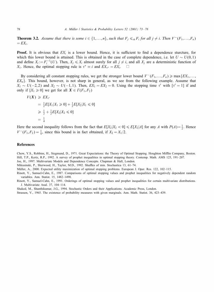
Theorem 3.2. Assume that there is some i ∈ {1; : : : ; n}, such that Fj6st Fi for all j 6= i. Then V−(F1; : : : ; Fn)= EXi.

Proof. It is obvious that EXi is a lower bound. Hence, it is su�cient to �nd a dependence sturcture, forwhich this lower bound is attained. This is obtained in the case of complete dependence, i.e. let U ∼ U (0; 1)and de�ne Xi :=F−1

i (U ). Then, Xj6Xi almost surely for all j 6= i, and all Xj are a deterministic function ofX1. Hence, the optimal stopping rule is �∗ ≡ i and EX�∗ = EXi.

By considering all constant stopping rules, we get the stronger lower bound V−(F1; : : : ; Fn)¿max{EX1; : : : ;EXn}. This bound, however, is not sharp in general, as we see from the following example. Assume thatX1 ∼ U (−2; 2) and X2 ∼ U (−1; 1). Then, EX1 = EX2 = 0. Using the stopping time �′ with [�′ = 1] if andonly if [X1¿ 0] we get for all X ∈ �(F1; F2)

V (X) ¿ EX�′

= 12E[X1|X1¿ 0] + 1

2E[X2|X16 0]

¿ 12 +

12E[X2|X26 0]

= 14

Here the second inequality follows from the fact that E[X2|X2¡ 0]6E[X2|A] for any A with P(A)= 12 . Hence

V−(F1; F2) = 14 , since this bound is in fact obtained, if X2 = X1=2.

References

Chow, Y.S., Robbins, H., Siegmund, D., 1971. Great Expectations: the Theory of Optimal Stopping. Houghton Mi�in Company, Boston.Hill, T.P., Kertz, R.P., 1992. A survey of prophet inequalities in optimal stopping theory. Contemp. Math. AMS 125, 191–207.Joe, H., 1997. Multivariate Models and Dependence Concepts. Chapman & Hall, London.Mikusinski, P., Sherwood, H., Taylor, M.D., 1992. Shu�es of min. Stochastica 13, 61–74.M�uller, A., 2000. Expected utility maximization of optimal stopping problems. European J. Oper. Res. 122, 102–115.Rinott, Y., Samuel-Cahn, E., 1987. Comparisons of optimal stopping values and prophet inequalities for negatively dependent randomvariables. Ann. Statist. 15, 1482–1490.

Rinott, Y., Samuel-Cahn, E., 1991. Orderings of optimal stopping values and prophet inequalities for certain multivariate distributions.J. Multivariate Anal. 37, 104–114.

Shaked, M., Shanthikumar, J.G., 1994. Stochastic Orders and their Applications. Academic Press, London.Strassen, V., 1965. The existence of probability measures with given marginals. Ann. Math. Statist. 36, 423–439.