Branching Processes, Martingales, Kingman’s

Subadditive Ergodic Theorem, and some applications

Sascha Troscheit

Department of Pure Mathematics, University of Waterloo, Waterloo, Ont., N2L 3G1, Canada

stroscheit@uwaterloo.ca

October 18, 2017

Abstract

These are the lecture notes for a short learning seminar given at the Department ofPure Mathematics, University of Waterloo.

Branching processes are stochastic processes often used to model reproduction andwere first developed to study effects in populations such as extinction of surnames andBrownian motion. However, these models have applications across a whole range of puremathematics and have been employed in solving problems in analysis, combinatorics,number theory, and group theory. In this series of seminars we take a probabilisticand dynamical view on several types of branching processes and study basic propertiessuch as the change of number of descendants. To do this we will use two tools, thetheory of martingales and ergodic theory, each of which become applicable in differentsituations:

• Classical branching process are often martingales and we will state and applythe martingale convergence theorems to define several geometrically interestingmeasures with applications to models such as percolation.

• For some modern branching processes, we state and prove a version of Kingman’ssubadditive ergodic theorem. This theorem is a very powerful tool in probabilityand dynamical systems with many applications to other fields such as numbertheory. We will apply this theorem to those branching processes to obtain someinteresting, albeit implicit, results and discuss some open problems for these pro-cesses.

1

Contents

1 Classical Branching processes 31.1 Galton–Watson Process . . . . . . . . . . . . . . . . . . . . . . . . . . . . . . 31.2 Probability Generating Function . . . . . . . . . . . . . . . . . . . . . . . . . 4

2 Martingales and Convergence Theorems 72.1 Doob’s Martingale convergence theorems . . . . . . . . . . . . . . . . . . . . . 82.2 Application to Galton–Watson processes . . . . . . . . . . . . . . . . . . . . . 9

3 Finer Information on the number of descendants 123.1 Application: Mandelbrot percolation (yet again) . . . . . . . . . . . . . . . . 14

4 Kingman’s Subadditive Ergodic Theorem 154.1 Fekete’s Lemma . . . . . . . . . . . . . . . . . . . . . . . . . . . . . . . . . . . 154.2 Kingman’s Subadditive Ergodic Theorem (at last) . . . . . . . . . . . . . . . 164.3 An Application . . . . . . . . . . . . . . . . . . . . . . . . . . . . . . . . . . . 18

5 V -variable branching processes 18

2

1 Classical Branching processes

Branching processes are stochastic processes that capture a ‘population’ where each ‘indi-vidual’ has a given distribution of producing ‘descendants’. In effect, they are random trees,where each node has a random number of descendants. The archetypal of such branchingprocess is called the Galton–Watson process and assumes that the offspring of an individualis independent and identical in distribution for every individual. We will analyse Galton–Watson processes in this section and continue exploring other branching processes in latersections, following an approach similar to Athreya [AN72]. To start, we recall the definitionof a tree and its boundary1.

Definition 1.1. Let Λ be a countable index set and let Λ∗ =⋃∞i=1 Λi be the set of finite

words over Λ. A tree τ (over Λ) is a subset of Λ∗ such that:

• For every v ∈ τ there exists λ ∈ Λ such that vλ ∈ τ .

• For every v ∈ τ of length greater than one, there exist λ ∈ Λ and w ∈ τ such thatv = wλ.

We note that some authors prefer rooted trees, in which case one would require theempty word to be in τ , acting as the root of the entire tree. Contrary to those authors wewill allow “empty trees”, i.e. τ = ∅ and random forests.

Definition 1.2. The (Gromov) boundary ∂τ of a tree τ are all infinite words v ∈ ΛN suchthat every finite restriction is in τ , i.e. v|k = v1v2 . . . vk ∈ τ for all k ∈ N.

1.1 Galton–Watson Process

We capture the distribution of offspring that an individual produces as a probability vector,called the offspring distribution.

Definition 1.3. The offspring distribution is the probability vector ~θ = (θ0, θ1, . . . ), where∑∞i=0 θi = 1. If additionally θ0 +θ1 < 1, we refer to ~θ as a non-trivial offspring distribution.

Let Xji be the random variable such that PXj

i = k = θk. In particular, Xji are pairwise

independent and have the same distribution. We write X for a generic copy of that randomvariable.

Definition 1.4. The sequence of random variables (Z0, Z1, . . . ) is called a Galton–Watsonprocess if Z0 = X0

0 and

Zi+1 =

Zi∑j=1

Xji+1.

This model was originally proposed by to study the extinction of surnames by Sir FrancisGalton. He posed his question in the Educational Times in 1873, to which Rev. HenryWatson replied. Later they published a join article on the extinction of families [GW75].Clearly, if there exists k such that Zk = 0 we must have Zl = 0 for all l ≥ k and this extinctionis what originally motivated Galton. Similarly, the first question we shall attempt to answeris:

1So far, we are not using this definition and it may get deleted or moved later.

3

Question 1.5. Given an offspring distribution ~θ, what is the probability that the associatedGalton–Watson process becomes extinct? That is, we aim to determine

PZk = 0 for some k.

Alternatively, we can define the k-th random variable in the Galton–Watson process asthe number of words of length k in a random tree where each node v ∈ τ has offspringdistribution according to τ , that is, for all v ∈ τ ,

θk = P#λ ∈ Λ | vλ ∈ τ = k.

By our definition of trees, there is a slight issue comparing offspring in this way: no nodecan have zero children and τ only contains nodes with children. We shall gloss over this factnow and put it on a formal footing later.

To determine when a Galton–Watson process ‘dies out’ we will use a powerful tool calledthe probability generating function.

1.2 Probability Generating Function

The probability generating function of a discrete random variable is a power series represen-tation that ‘encodes’ many useful properties of the random variable. It is defined in termsof expectations, and we write E(X) =

∫ΩX(ω)dP(ω) for the expectation of X with respect

to some probability space (Ω,P). We will ignore the issue of measurability entirely as allthe random variables we will consider are (Borel) measurable.

Definition 1.6. The probability generating function f(X, s) of a discrete random variableX is defined as

f(X, s) = E(sX) =

∞∑i=0

PX = isi.

For simplicity, we will often write f(s) if X = Z0 is the random variable associated with agiven offspring distribution for a Galton–Watson process.

Example. Let ~θ = p, 1 − p, 0, 0, . . . for some 0 ≤ p ≤ 1. If p = 1, then clearly theGalton–Watson tree τ is empty almost surely. Similarly, if p = 0, then Zk = 1 for all kalmost surely. If 0 < p < 1, then Zk = 1 with probability (1− p)k+1 and hence the processdies out almost surely. Since this behaviour is so simple and uninformative we refer to thecase θ0 + θ1 = 1 as a trivial Galton–Watson process. In both of these cases the probabilitygenerating function is linear, f(s) = p+ (1− p)s, with f(0) = θ0 and f(1) = 1.

As it turns out, the last two facts hold in much greater generality, but the generatingfunction is now strictly convex, a fact that we will use later on. We write f (k) for thek-th derivative of f and fk(s) for the k-fold composition of the map f , i.e. f1(s) = f(s),f2(s) = (ff)(s), f3(s) = (fff)(s), et cetera. Combining composition and differentiation,

we write f(l)k (s) = (dl/dsl)fk(s).

Theorem 1.7. Let ~θ be a non-trivial offspring distribution with associated random variableX. The following statements hold for its generating function f(s).

1. f(0) = θ0 and lims1 f(s) = 1.

2. f(s) is smooth on [0, 1) and f (k)(s) is continuous at s = 1 if f (k)(1) <∞.

4

3. The offspring distribution can be recovered by

PX = k =f (k)(0)

k!.

4. The mean of X is m = E(X) = f (1)(1).

5. Assume E(X) is finite. Then the variance Var(X) = E((X −m)2) is

Var(X) = f (2)(1) +m−m2.

6. f(s) is strictly convex and increasing in s on [0, 1]

7. If m ≤ 1, then f(t) > t for all t ∈ [0, 1). If m > 1, then there exists a unique q ∈ [0, 1)such that f(q) = q.

8. If t ∈ [0, q), then fk(t) q as k →∞. If t ∈ (q, 1), then fk(t) q as k →∞.

Proof.

1. The first claim is trivial and the second follows from Abel’s theorem.

2. Smoothness arises from the non-negativity of entries in the sum (and Abel’s theoremfor s = 1).

3. Simple computation. Differentiating once we get

f (1)(s) =

∞∑i=1

θi i si−1 =

∞∑i=0

θi i si−1,

differentiating again,

f (2)(s) =

∞∑i=0

θi i (i− 1) si−2,

and in general

f (k)(s) =

∞∑i=0

θi i (i− 1) . . . (i− k + 1)si−k.

Setting s = 0 gives the desired result.

4. Simple computation f (1)(1) =∑∞i=1 θi i 1i = E(X).

5. We compute

Var(X) = E((X −m)2) =

∞∑i=0

θi(i−m)2 =

∞∑i=0

θi i2 +

∞∑i=0

θim2 − 2

∞∑i=0

θimi

=

∞∑i=0

θi i2 + (−m+m)−m2 =

∞∑i=0

θi i2 −

∞∑i=0

θi i+m−m2

=

∞∑i=0

θi i(i− 1) +m−m2 = f (2)(1) +m−m2.

5

6. Positive constants and non-triviality imply f (1)(s) > 0 and f (2)(s) > 0, thus f(s) isstrictly increasing and convex.

7. Follows from 6.

8. Clearly 0 ≤ t < q gives t < f(t) < f(q) and iterating gives

t < f(t) < f2(t) < f3(t) < · · · < fk(t) < f(q) = q.

By continuity fk(t) L for some L that satisfies f(L) = L. But q is the least rootand thus L = q. The other limit follows similarly.

1.2.1 Linking the generating function to Zk

There is a strong connection between iterates of the probability generating function and theGalton–Wason process Zk. Consider

f(Z1, s) = f( Z0∑i=1

Xi1, s)

= E(s∑Z0i=1X

i1)

= E(E(sX11 sX

21 . . . sX

Z01 | Z0))

= E((E(sX11 ))Z0) = E(f(X1

1 , s)X1

0 )

= f(X, f(X, s)) = f2(X, s).

This can be extended (in the obvious way) for all k ∈ N and f(Zk, s) = fk(X, s).

Theorem 1.8. Let Zk be a Galton–Watson process with mean m = E(Z0) = E(X) <∞.Then E(Zk) = mk.

Proof. From Theorem 1.7 and the chain rule we deduce,

f(1)1 (Zk, s) = f

(1)k (X, s) = f

(1)k−1(X, f1(X, s)) · f (1)

1 (X, s)

= f(1)k−2(X, f2(X, s)) · f (1)

1 (X, f1(X, s)) · f (1)1 (X, s)

= f (1)(X, fk−1(X, s)) · f (1)(X, fk−2(X, s)) · . . . · f (1)(X, s).

But then,

E(Zk) = f(1)1 (Zk, 1) = f (1)(X, fk−1(X, 1)) · . . . · f (1)(X, 1) = [f (1)(X, 1)]k = mk.

Theorem 1.9. Let Zk be a Galton–Watson process and let q ∈ [0, 1] be the smallestsolution to f(Z0, q) = q. Then the probability of extinction of the process is q,

PZk = 0 | for some k = q

Proof. First note that

PZk = 0 | for some k = limk

PZk = 0 = limkf(Zk, 0)

and so by Lemma 1.7,

PZk = 0 | for some k = limkfk(X, 0) = q.

6

1.2.2 Example: Mandelbrot percolation

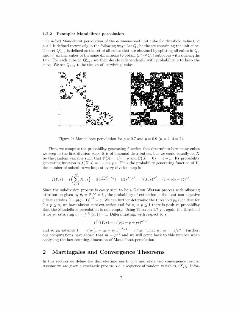
The n-fold Mandelbrot percolation of the d-dimensional unit cube for threshold value 0 <p < 1 is defined recursively in the following way: Let Q1 be the set containing the unit cube.The set Q′n+1 is defined as the set of all cubes that are obtained by splitting all cubes in Qninto nd smaller cubes of the same dimensions to obtain (nd ·#Qn) subcubes with sidelengths1/n. For each cube in Q′n+1 we then decide independently with probability p to keep thecube. We set Qn+1 to be the set of ‘surviving’ cubes.

Figure 1: Mandelbrot percolation for p = 0.7 and p = 0.9 (n = 2, d = 2).

First, we compute the probability generating function that determines how many cubeswe keep in the first division step. It is of binomial distribution, but we could equally let Xbe the random variable such that PX = 1 = p and PX = 0 = 1 − p. Its probabilitygenerating function is f(X, s) = 1− p+ p s. Thus the probability generating function of Y ,the number of subcubes we keep at every division step is

f(Y, s) = f( nd∑i=1

Xi, s)

= E(s∑nd

i=1Xi) = E(sX)nd

= f(X, s)nd

= (1 + p(s− 1))nd

.

Since the subdivision process is easily seen to be a Galton–Watson process with offspringdistribution given by θi = PY = i, the probability of extinction is the least non-negative

q that satisfies (1+p(q−1))nd

= q. We can further determine the threshold p0 such that for0 < p ≤ p0 we have almost sure extinction and for p0 < p ≤ 1 there is positive probabilitythat the Mandelbrot percolation is non-empty. Using Theorem 1.7 yet again the thresholdis for p0 satisfying m = f (1)(Y, 1) = 1. Differentiating, with respect to s,

f (1)(Y, s) = ndp(1− p+ ps)nd−1

and so p0 satisfies 1 = ndp0(1 − p0 + p0 1)nd−1 = ndp0. That is, p0 = 1/nd. Further,

our computations have shown that m = pnd and we will come back to this number whenanalysing the box-counting dimension of Mandelbrot percolation.

2 Martingales and Convergence Theorems

In this section we define the discrete-time martingale and state two convergence results.Assume we are given a stochastic process, i.e. a sequence of random variables, (Xi)i. Infor-

7

mally, a martingale is a process where, given information about all previous outcomes, theexpectation of the next outcome is the current value.

For martingales we will also need the notion of conditional expectation.

Definition 2.1 (Conditional expectation). Let X be a random variable and A ′ ⊆ A be aσ-algebra. The conditional expectation of X given A ′, denoted by E(X|A ′), is any A ′-measurable function Ω→ R satisfying∫

A′E(X|A ′)dP =

∫A′XdP

for all A′ ∈ A ′.

The conditional expectation can be interpreted as the expectation with the ‘knowledge’of events in the σ-algebra A ′. The ‘finer’ the σ-algebra, the better our prediction of the out-come. As an example, if A ′ = ∅,Ω we have no knowledge and the conditional expectationis a constant function E(X|A ′) = E(X). However, if A ′ = A , we have ‘total knowledge’and E(X|A ′) = X. Given a random variable, we define 〈X〉, the σ-algebra generated by X,to be the smallest σ-algebra such that X is Borel measurable.

It is important to note that P is a measure on the event space Ω. Given a fixed r.v. wemight instead want to talk about the distribution of measurements. The distribution PX issimply the image of the measure P under X, i.e. PX(A) = P(X ∈ A) for all A ⊂ R, whichis itself a measure.

Definition 2.2. A discrete stochastic process (Mi)i is called a (discrete-time) martingaleif all Mi are integrable and

E(Mi+1 | 〈M1,M2, . . . ,Mi〉) = Mi for all i.

Equivalently,E(Mi+1 −Mi | 〈M1,M2, . . . ,Mi〉) = 0 for all i.

Similarly, a stochastic process is called a submartingale if it satisfies

E(Mi+1 | 〈M1,M2, . . . ,Mi〉) ≥Mi for all i,

and a supermartingale if

E(Mi+1 | 〈M1,M2, . . . ,Mi〉) ≤Mi for all i.

We note that every martingale is also a supermartingale and submartingale.

2.1 Doob’s Martingale convergence theorems

The first convergence result we mention is due to Doob about pointwise convergence and aproof can be found in [Wil91].

Theorem 2.3. Let (Mi) be a supermartingale in L1, that is supi E(|Mi|) < ∞. Then thepointwise limit M = limi→∞Mi exists almost surely and E(M) <∞.

Corollary 2.4 (Non-negative Martingale Convergence Theorem2). Let (Mi) be a non-negative supermartingale. Then the pointwise limit M = limi→∞Mi exists almost surely.

2The name of this theorem is also the only theorem known to the author for which the number of wordsin English necessary to state the theorem adequately is no greater than the number of words in its title.The non-negative martingale convergence theorem: non-negative martingales converge.

8

Proof. Since E(|Mi|) = E(Mi) ≤ E(M0), the process is in L1 and we can apply the pointwiseMartingale convergence theorem.

Example 2.5. Let S0 be my accumulated wealth and assume that it is positive and finite.Assume further, that I have quit my job and will not have any income anymore from anysource. Also, assume that I have no expenditures and do not consume food of any kind. Iturn to the only thing left: gambling. Note that, even though we do not know what game Iam playing, we can say that the games are at best fair games and my wealth after the k-thgame only depends on the wealth I have had before. In other words, E(Sk | 〈Sk−1〉) ≤ Sk−1.Because of my bad credit history, I am not eligible for any credit. Thus, assume that Sk ≥ 0for all k, i.e. I stop playing if I run out of money. My wealth therefore is a non-negativemartingale and we can apply Theorem 2.3 and conclude that my wealth converges almostsurely, independent of any gambling strategy, almost surely I will stop playing and end upwith a fixed amount of wealth. Knowing my habits, Sk = 0, for some big enough k.

We note that these two results do not imply convergence in L1, i.e. E(|Mi −M |) maynot tend to 0 as i→∞. We will shortly see an illuminating example of this but if we wantthis convergence, or uniform convergence, we need stronger assumptions and state anotherresult by Doob, a proof of which can also be found in [Wil91].

Theorem 2.6. Let (Mi) be a supermartingale such that supi E|Mi|p < ∞ for some p > 1.Then there exists a random variable M ∈ Lp(Ω,R) such that

Mi →a.s. X and

∫Ω

|Mi −M |pdP→ 0.

In particular, E(|Mi|p)→ E(|M |p).

2.2 Application to Galton–Watson processes

The first of the two convergence theorems is useful if you only require almost sure convergenceand do not need to know anything about the limit. As an example, we look at a processthat we can obtain from the Galton–Watson process, called the normalised Galton–Watsonprocess.

Definition 2.7. Let ~θ be a non-trivial offspring distribution with associated Galton–Watsonprocess (Zk) with finite mean, m = E(Z0). The normalised Galton–Watson process is

Wk = Zk/mk.

We immediately see that E(Wk) = 1 for all k > 0.

Lemma 2.8. The stochastic process (Wi) is a non-negative martingale and thus convergesalmost surely to some random variable W with finite expectation.

Proof. Since Zn ≥ 0 and by non-triviality the mean m is positive, we also have Wi ≥ 0 forall i. It remains to check that (Wk) is a martingale.

E(Wk | 〈W1, . . . ,Wk−1〉) = E(Zk/mk | 〈Z1, . . . , Zk−1〉)

= E(Zk/mk | 〈Zk−1〉)

= E(

1/mk

Zk−1∑i=1

Xik

∣∣∣ 〈Zk−1〉)

9

= E(

1/mkZk−1

∣∣∣ 〈Zk−1〉)E(Xi

k)

= (Zk−1/mk−1)E(Z0)/m = Wk−1,

as required. The convergence follows from Corollary 2.4.

This convergence allows us to conclude that almost every Galton Watson process satisfiesC−1ω mk ≤ Zk ≤ Cωm

k for some random Cω and big enough k. However, Cω = 0 almostsurely, is not excluded and would give a fairly trivial result. We note further, that such aGalton–Watson process may not even converge in L1. Let ~θ be such that its mean satisfiesm = 1. We have already learnt that Zn = 0 for big enough n is an almost sure event.Its normalised Galton–Watson process (Wn) then coincides with (Zn) and both have unitexpectation for all n. But almost sure extinction means that E(W ) = 0 and so

E(|Wn −W |) = E(|Zn − Z|) = E(Zn) = 1 6→ 0.

When it comes to Lp convergence, the easiest case to check is usually p = 2, since

E(M2n) = E(M2

0 ) +

n∑i=1

E((Mi −Mi−1)2).

However, for Galton–Watson processes there is an even more convenient way to determinethe second moment. Let ~θ be any offspring distribution, we observe that

f (2)(X, s) =

∞∑i=2

θi(i)(i− 1)si−2 =

∞∑i=0

θi(i)(i− 1)si−2 =

∞∑i=0

θi i2 si−2 − f (1)(X, s).

This holds in general and we find

E((Zk −mk)2) =

∞∑i=0

PZk = i(i−mk)2

=

∞∑i=0

PZk = i i2 +

∞∑i=0

PZk = i(mk)2 − 2

∞∑i=0

PZk = i imk

=

∞∑i=0

PZk = i i2 + (mk)2 − 2mkf(Zk, 1)

=

∞∑i=0

PZk = i i2 −m2k

= f(2)k (X, 1) + f

(1)k (X, 1)−m2k

= f(2)k−1(X, f(X, 1))(f (1)(X, 1))2 + f

(1)k−1(X, f(X, 1))f (2)(X, 1) +mk −m2k

= f(2)k−1(X, 1)m2 + f

(1)k−1(X, 1)f (2)(X, 1) +mk −m2k

= f(2)k−1(X, 1)m2 +mk−1f (2)(X, 1) +mk −m2k

= (f(2)k−2(X, 1)m2 +mk−2f (2)(X, 1))m2 +mk−1f (2)(X, 1) +mk −m2k

= f(2)k−2(X, 1)m4 + f (2)(X, 1)(mk−1 +mk) +mk −m2k

= f(2)k−3(X, 1)m6 + f (2)(X, 1)(mk−1 +mk +mk+1) +mk −m2k

= f (2)(X, 1)(mk−1 +mk +mk+1 + · · ·+m2k−2) +mk −m2k

10

Now Var(X) = f (2)(X, 1) +m−m2 and so

Var(Zk) = E((Zk −mk)2) = Var(X)mk−1(1 +m+ · · ·+mk−1) = Var(X)mk−1mk − 1

m− 1.

So,

Var(Wk) =

(1

mk

)2

Var(Zk) = Var(X)mk − 1

mk (m2 −m)= Var(X)

1−m−k

m(m− 1),

which is bounded above for m > 1. This means that we can apply the second martingaleconvergence theorem and there exists W ∈ L2 such that Wk →W almost surely. Moreover,since Wk is non-negative, 1 = E(Wk) → E(W ) and thus there exists positive probabilitythat Wk mk. Further, since PW = ∞ = 0, we can claim that Wk converges to somepositive real number almost surely, conditioned on non-extinction.

Box-counting dimension of Mandelbrot percolation This can now be applied tocalculate the box-counting dimension of Mandelbrot percolation.

Definition 2.9. Let (M, d) be a totally bounded metric space. Denote by Nδ(M) the leastnumber of sets of diameter δ > 0 needed to cover M. The box-counting dimension of M isdefined as

dimB M = limδ→0

logNδ(M)

− log δ.

If the limit does not exist we talk about upper and lower box-counting dimension, taking theupper and lower limit, respectively.

Assume that p > nd, so that there is a positive probability that the limit set is non-empty. One can easily see that the least number of sets of diameter δ = n−k is comparable tothe number of subcubes at stage k. Since those are Galton–Watson processes with boundedvariance, the above result can be applied to give #Qk mk. Thus

logNn−k(M(ω))

− log n−k≤ logCωm

k

k log n=

logCωk log n

+log(p nd)

log n

for some Cω that is almost surely positive and finite, conditioned on non-extinction. Asimilar lower bound holds and upon taking limits we conclude that the almost sure box-counting dimension of Mandelbrot percolation is log(ndp)/ log n. The keen observer mightnote that we only looked at δ = n−k, however, this does not produce any issues as thenumber of subcubes surviving is off by at most a fixed multiple to the least number ofcovering sets. We leave details to the reader.

2.2.1 Random Cascade Measure

The same process can be applied to labelled trees to generate a random measure on [0, 1]d

called the random cascade measure. Let X be a non-negative random variable with meanE(X) = n−d and consider a process similar to the Mandelbrot percolation. At each step wesubdivide a subcube into nd subcubes but instead of deleting cubes we associate a realisationof XC with each subcube C. Let C ⊂ Qk be a level k cube with address C1C2 . . . Ck. Wedefine its l-level mass by

ml(C) = XC1XC2

. . . XCk

∑D∈Qk+lDi=Ci1≤i≤k

Dk+1Dk+2 . . . Dk+l

11

Now ml(C) is a non-negative martingale and the pointwise convergence theorem tells usthat ml converges pointwise and it is easily verifiable that the limit m is indeed a measureon the unit cube. This random measure is the random cascade measure.

Let d = 1 and n = 2. That is, the subcubes are the dyadic intervals. Let X be a randomvariable with mean 1/2 and PX = 0 = 0. Consider the associated random cascademeasure and assume E(X logX) <∞. It can be shown that the associated random cascademeasure µ of the unit interval is almost surely positive. Without loss of generality we assumeµ([0, 1]) = 1 and set φ(x) = µ([0, x)) to be the cumulative probability distribution functionand note that it is strictly increasing (almost surely).

Now let F be any subset of the unit line, a question that is currently of active interestis what happens to the dimensions of F under the mapping φ, i.e. what is the relationshipbetween dimF and dimφ(F ).

3 Finer Information on the number of descendants

So far, we have learnt about the mean of the Galton–Watson process at step n, and achievedfiner almost sure results using martingales. In this section we will go back to the probabilitygenerating function to prove a Lemma due to Athreya [Ath94]. This Lemma will allow usto estimate the number of descendants at a given node and we will apply this to establish asimilar result as in [Tro17] but for Mandelbrot percolation. process.

We first introduce additional notation. Notice that f , the generating function, wasconvex and strictly increasing. Hence it is invertible with strictly increasing but concavederivative. We denote the inverse map of f by g and write gk for the k-th iterate of theinverse.

From now on we make an assumption that is somewhat stronger than the mean existing,namely that the generating function is defined on an interval greater than [0, 1]. We generallymake the assumption that there exists s0 > 1 such that f(s0) < ∞. This implies that f isdefined on [0, s0] and g on [f(0), f(s0)] = [θ0, f(s0)]. As a side-note, this further means thatthe mean is defined since s0 > 1 forces f (1)(1) <∞.

Lemma 3.1. Let f(s0) < ∞ for some s0 > 1. Then, for 1 ≤ s ≤ f(s0) and gk(s0) 1from above,

mk(gk(s)− 1) G(s),

where G(s) is the unique solution to G(f(s)) = mG(s) for 1 ≤ s ≤ f(s0). Further 0 <G(s) <∞ for all 1 < s ≤ f(s0) and G(1) = 0 and G′(1) = 1.

The proof is similar to the ones we have seen for the generating function and we omitdetails.

Lemma 3.2 ([Ath94, Theorem 4]). Let Zk be a Galton–Watson process with mean m =E(Xε) < ∞. Suppose that there exists t0 > 0 such that E(exp(t0Z1) | Z0 = 1) < ∞. Thenthere exists t1 > 0 such that

supk∈N

E(et1Wk

∣∣∣ Z0 = 1)<∞ (3.1)

Proof. By assumption, there exists some s0 = et0 > 1 such that f(s0) < ∞. Let K =f(s0) < ∞, we must have f2(s) ≤ K if 0 ≤ f(s) ≤ s0. Equivalently, 0 ≤ s ≤ g(s0) and ingeneral we get

fn(s) ≤ K if 0 ≤ s ≤ gn−1(s0).

12

Recall that Wk was the normalised Galton–Watson process and so

E(etWk

∣∣∣ Z0 = 1)

= fn

(etm

−k).

Thus,

E(etWk

∣∣∣ Z0 = 1)≤ K if t ≤ mk log gn−1(s0).

It is a simple argument, similar to Theorem 1.7, to establish that gk(t) → 1 for all t > 1where g is defined. We can therefore conclude that log gk(s0) ∼ gk(s0)− 1 and make use ofLemma 3.1, and have

mk log gk−1(s0)→ mG(s0),

which is positive and finite. Since, further gk(s0) > 1 for all k ≥ 1 we can choose

t1 = infkmk log gk−1(s0)

and the left-hand side of (3.1) is bounded by K.

With this technical lemma out of the way we can now focus our attention on an interestingconsequence with regards to the deviation from the mean number of children.

Theorem 3.3. Let Zk be a Galton–Watson process with non-trivial offspring distribution.Assume that there exists t0 such that E(exp(t0Z1) | Z0 = 1) < ∞. Let C > 0 and ε > 0 begiven. Then there exist t2 > 0 and D > 0 such that

PZk ≥ Cm(1+ε)k

≤ De−t2m

εk

.

That is, the probability that Zk exceeds Cm(1+ε)k decreases superexponentially.

Proof. Let t1 and K be given by Lemma 3.2. We use a standard Chernoff bound to obtain,

PZk ≥ Cm(1+ε)k

= P

Wk ≥ Cmεk

= P

exp (t1Wk) ≥ exp

(Ct1m

εk)

≤ E (exp (t1Wk))

exp (Ct1mεk)

= Ket2mεk

,

for t2 = Ct1, as required.

We can state an immediate corollary.

Corollary 3.4. Let Zk be a Galton–Watson process satisfying the conditions of Theorem 3.3.Let C > 0 and ε > 0 be given. Then,

PZk ≥ Cm(1+ε)k for some k ≥ l

≤∞∑k=l

De−t2mεk

≤ D′e−t2mεl

,

for some D′ > 0 independent of l.

13

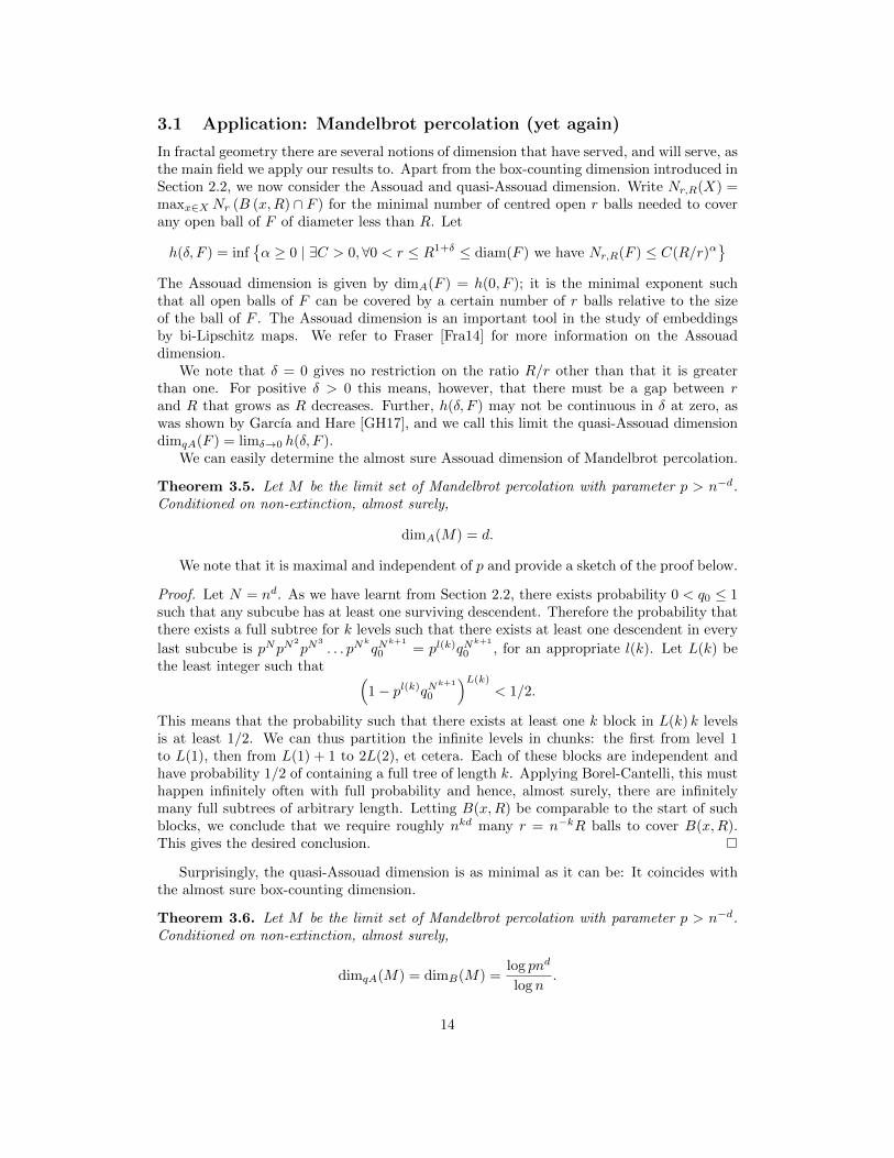
3.1 Application: Mandelbrot percolation (yet again)

In fractal geometry there are several notions of dimension that have served, and will serve, asthe main field we apply our results to. Apart from the box-counting dimension introduced inSection 2.2, we now consider the Assouad and quasi-Assouad dimension. Write Nr,R(X) =maxx∈X Nr (B (x,R) ∩ F ) for the minimal number of centred open r balls needed to coverany open ball of F of diameter less than R. Let

h(δ, F ) = infα ≥ 0 | ∃C > 0,∀0 < r ≤ R1+δ ≤ diam(F ) we have Nr,R(F ) ≤ C(R/r)α

The Assouad dimension is given by dimA(F ) = h(0, F ); it is the minimal exponent suchthat all open balls of F can be covered by a certain number of r balls relative to the sizeof the ball of F . The Assouad dimension is an important tool in the study of embeddingsby bi-Lipschitz maps. We refer to Fraser [Fra14] for more information on the Assouaddimension.

We note that δ = 0 gives no restriction on the ratio R/r other than that it is greaterthan one. For positive δ > 0 this means, however, that there must be a gap between rand R that grows as R decreases. Further, h(δ, F ) may not be continuous in δ at zero, aswas shown by Garcıa and Hare [GH17], and we call this limit the quasi-Assouad dimensiondimqA(F ) = limδ→0 h(δ, F ).

We can easily determine the almost sure Assouad dimension of Mandelbrot percolation.

Theorem 3.5. Let M be the limit set of Mandelbrot percolation with parameter p > n−d.Conditioned on non-extinction, almost surely,

dimA(M) = d.

We note that it is maximal and independent of p and provide a sketch of the proof below.

Proof. Let N = nd. As we have learnt from Section 2.2, there exists probability 0 < q0 ≤ 1such that any subcube has at least one surviving descendent. Therefore the probability thatthere exists a full subtree for k levels such that there exists at least one descendent in every

last subcube is pNpN2

pN3

. . . pNk

qNk+1

0 = pl(k)qNk+1

0 , for an appropriate l(k). Let L(k) bethe least integer such that (

1− pl(k)qNk+1

0

)L(k)

< 1/2.

This means that the probability such that there exists at least one k block in L(k) k levelsis at least 1/2. We can thus partition the infinite levels in chunks: the first from level 1to L(1), then from L(1) + 1 to 2L(2), et cetera. Each of these blocks are independent andhave probability 1/2 of containing a full tree of length k. Applying Borel-Cantelli, this musthappen infinitely often with full probability and hence, almost surely, there are infinitelymany full subtrees of arbitrary length. Letting B(x,R) be comparable to the start of suchblocks, we conclude that we require roughly nkd many r = n−kR balls to cover B(x,R).This gives the desired conclusion.

Surprisingly, the quasi-Assouad dimension is as minimal as it can be: It coincides withthe almost sure box-counting dimension.

Theorem 3.6. Let M be the limit set of Mandelbrot percolation with parameter p > n−d.Conditioned on non-extinction, almost surely,

dimqA(M) = dimB(M) =log pnd

log n.

14

Again, we only sketch the proof, a full version of which can be found in [Tro17].

Proof. Let δ > 0 and assume for a contradiction that there exists ε > 0 such that dimqA(M) ≥dimB(M) + ε with positive probability. Thus we should be able to find a sequence ofballs B(x,R) such that the minimal number of covering sets exceeds (pnd)(1+ε)k, wherek ≥ logR/ log r. This is equivalent to finding infinitely many subcubes in the Mandelbrot

percolation at levels lk with more than (pnd)(1+ε) subcubes at levels exceeding l1+δ′

k forsome δ′ > 0 only dependent on δ. We know from Corollary 3.4 that the probability of thisoccurring decreases superexponentially. However, the number of descendants grows at mostexponentially since they are bounded by nd children at every step and we get

P ∃k-level subcube with “too many” descendants ≤(nd)kD′e−t2m

ε(1+δ′)k

and we note that summing the right-hand term over k is finite. But then the probabilitythat there are infinitely many levels that contain such a full enough subtree is zero by theBorel–Cantelli Lemmas, contradicting the positive measure assumption.

4 Kingman’s Subadditive Ergodic Theorem

Let (Ω, µ) be a probability space. Consider the surjective map T : Ω → Ω. We assumethat T is invariant with respect to µ, i.e. µ(A) = µ(T−1A) for all measurable A ⊆ Ω. LetF : Ω → R be a real-valued measurable function. We say that T is ergodic with respect toµ if A = T−1A implies µ(A) = 0 or µ(Ω \A) = 0 for all measurable A ⊆ Ω.

The famous Birkhoff’s Ergodic Theorem then states that for µ-almost every ω ∈ Ω,

1

n

n∑j=1

F (T j(ω))→∫f dµ,

if T is ergodic. Informally, we say that the time average converges to the space average forobservable F .

4.1 Fekete’s Lemma

To motivate Kingman’s subadditive theorem, consider the following well known result onsub-additive sequences. Let (ai)

∞i=1 be a real-valued sequence such that an+m ≤ an + am.

We call any such sequence subadditive. Fekete’s Lemma states that an/n converges if (ai)∞i=1

is subadditive.

Lemma 4.1 (Fekete’s Lemma). Let (ai)∞i=1 be a subadditive sequence. Then,

ann→ lim inf

i→∞

aii∈ [−∞,∞).

While the proof does not help us for Kingman’s subadditive ergodic theorem, it isstraightforward and we include it for completeness.

Proof. Let q ∈ N. Then, for every n, there exists a unique pn ∈ N and rn ∈ 0, 1, . . . , p− 1such that n = pq + r. Therefore, using subadditivity,

ann

=apnq+rnpnq + rn

15

≤ apnq + arnpnq

≤ pnaq + arnpnq

and therefore, taking the upper limit,

lim supn→∞

ann≤ lim sup

n→∞

pnaq + arnpnq

=aqq.

But this holds for any q ∈ N and so, in particular, lim infi→∞ ai/i is a (finite) upperbound.

4.2 Kingman’s Subadditive Ergodic Theorem (at last)

In this section we state and prove Kingman’s subadditive theorem. The original theorem isdue to Kingsman [Kin73] and the short proof we present is due to Steele [Ste89].

Theorem 4.2. Let T be a µ-invariant surjective transformation on Ω and let gn be asequence of integrable sub-additive functions,

gn+m(ω) ≤ gn(ω) + gm(Tnω). (4.1)

Then, for µ-almost every ω ∈ Ω,

limn→∞

gn(ω)

n= g(ω) ≥ −∞,

where g is an invariant function. Further, if T is also ergodic, then g is constant almostsurely.

Proof. Instead of gn we could consider the function

gn(ω) = gn(ω)−n−1∑i=1

g1(T iω). (4.2)

Using the subadditivity this implies gn ≤ 0 and further gn satisfies the same subadditivitycondition of equation 4.1. As we are interested in gn/n, we see that the second term in (4.2),when normalised by n, converges for almost every ω due to Birkhoff’s Ergodic Theorem.Therefore, gn/n converges if and only if gn/n converges. We can therefore, without loss ofgenerality, assume that gn is non-positive.

For definitiveness, we define g(ω) = lim infn→∞ gn(ω)/n. We observe that g is an invari-ant function with respect to T . Since gn+1(ω)/n ≤ g1(ω)/n+ gn(T (ω))/n we take the lowerlimit and obtain g(ω) ≤ g(T (ω)). But then

ω ∈ Ω | g(ω) ≥ α ⊆ ω ∈ Ω | g(T (ω)) ≥ α = T−1 ω ∈ Ω | g(ω) ≥ α

and so the sets on the left-hand side and right-hand differ by at most a set of zero measure,since T is measure preserving. This means that g(ω) = g(T (ω)) almost surely. Further, ifT is ergodic with respect to µ, the intersection of the two sets must have measure zero orone. But then there exists some “jump value” α and g(ω) = α almost surely. By takingcountable intersections of full measure subsets of Ω we can thus, without loss of generality,assume that g(T k(ω)) = g(ω) for all k.

16

To get the required convergence results we will employ a few tricks. The first one concernsthe lower bound. Nothing is preventing g = −∞ for some, or all ω ∈ Ω (nor did we claim so),and we will circumvent the slight issue this is presenting by defining Gb(ω) = min −b, g(ω)for b ≥ 0. Now, let ε > 0 and b ≥ 0 be given. For every N ∈ N we define the bad words

Bb,ε(N) = ω ∈ Ω | gl(ω)/l > Gb(ω) + ε for all 1 ≤ l ≤ N .

Correspondingly we let Sb,ε(N) = Ω \Bb,ε(N) be the set of splendid words.Consider an arbitrary ω ∈ Ω and let n > 1 be given. We consider the integer set

1, 2, 3, . . . , n − 1 and will decompose it into several disjoint sets of three different types:τ1, τ2, and τ3. This follows the following algorithm.

1. Set k = 1.

2. Consider ω′ = T k(ω):

(a) If ω′ ∈ Bb,ε(N) add the singleton set k to τ1. Go to Step 3.

(b) If ω′ ∈ Sb,ε(N), there exists l such that

gl(Tk(ω)) ≤ l(Gb(T k(ω)) + ε) = l(Gb(ω) + ε).

If there are multiple, consider the least l and evaluate l + k:

i. If l + k < n, add the set k, k + 1, . . . , k + l − 1 to τ2. Go to Step 3.

ii. If l + k ≥ n, add the singleton set k to τ3. Go to Step 3.

3. Check whether there are any integers in 1, . . . , n− 1 not contained in any of τ1, τ2,or τ3. If there is, let k be the least such integer and go to Step 2. Otherwise, terminatethe algorithm.

Let j be the number of sets in class τ2 and write li for the number of elements in eachof the j sets. Further. we write ki for the least element in each of these sets. Note thatwe can use the subadditivity to decompose gn(ω) as the sum of values at each of the pairsdetermined above, that is

gn(ω) ≤j∑i=1

gli(Tki(ω)) +

#τ1∑i=1

g1(T ki(ω)) +

#τ3∑i=1

g1(T ki(ω)) ≤j∑i=1

gli(Tki(ω)),

where the last inequality holds as gn(ω) ≤ 0. But since we know that T ki(ω) is splendid wecan further write

gn(ω) ≤j∑i=1

li(Gb(ω) + ε) ≤ Gb(ω)

n∑i=1

li + nε, (4.3)

where we take li = 1 for all i > j. Note further that by virtue of construction

n ≤j∑i=1

li +

n∑i=1

χBb,ε(N)(Ti(ω)) +N

and so,

1

n

j∑i=1

li ≥ 1− N

n− 1

n

n∑i=1

χBb,ε(N)(Ti(ω))

17

Taking the lower limit and applying Birkhoff’s Ergodic Theorem we obtain, for almost everyω ∈ Ω,

lim infn→∞

1

n

n∑i=1

li ≥ 1− limn→∞

1

n

n∑i=1

χBb,ε(N)(Ti(ω)) = 1− E

(χBb,ε(N)

)= 1− µ (Bb,ε(N))

Combining this with the upper bound in (4.3) we get, almost surely,

lim supn→∞

gn(ω)

n≤ Gb(ω)(1− µ(Bb,ε(N)) + ε ≤ Ga(ω)(1− µ(Bb,ε(N)) + ε

for all a ≤ b.We are now almost done. First letting N →∞ gives

lim supn→∞

gn(ω)/n ≤ Ga(ω) + ε,

which holds for all a ≥ 0 and ε > 0. Thus,

lim supn→∞

gn(ω)/n ≤ lim infn→∞

gn(ω)/n = g(ω),

almost surely, as required.

4.3 An Application

Let Mλ be n×n matrices, indexed by some λ ∈ Λ. Let µ be a probability measure supportedon Λ. Let Ω = ΛN be the set of infinite sequences over Λ and set P = µN. It is easy to checkthat P is invariant with respect to T (ω) = T (ω1ω2 . . . ) = ω2ω3 . . . . Slightly less trivial, themeasure P is also ergodic with respect to T . Let ‖.‖ be any submultiplicative matrix norm.Then,

‖Mω1Mω2 . . .Mωk‖1/k → c ∈ [0,∞) as k →∞ (a.s.). (4.4)

This can quickly be proved by letting gn(ω) = log‖Mω1Mω2

. . .Mωn‖ which is subadditiveby the submultiplicativity of the norm.

gn+m(ω) = log‖Mω1Mω2

. . .Mωn+m‖

≤ log‖Mω1. . .Mωn‖+ log‖Mωn+1

. . .Mωn+m‖

= gn(ω) + gm(Tnω).

Hence, gn(ω)/n converges almost surely in [−∞,∞), taking exponentials and noting that Twas ergodic, the limit of (4.4) is non-negative and constant almost surely.

5 V -variable branching processes

References

[AN72] K. B. Athreya and P. E. Ney. Branching processes. Springer-Verlag, New York-Heidelberg, 1972. Die Grundlehren der mathematischen Wissenschaften, Band 196.

[Ath94] K. B. Athreya. Large deviation rates for branching processes. I. Single type case.Ann. Appl. Probab., 4, no. 3, (1994), 779–790.

18

[Fra14] J. M. Fraser. Assouad type dimensions and homogeneity of fractals. Trans. Amer.Math. Soc., 366, (2014), 6687–6733.

[GH17] I. Garcıa and K. Hare. Properties of Quasi-Assouad dimension. ArXiv e-prints.

[GW75] F. Galton and H. W. Watson. On the probability of the extinction of families.Journal of the Royal Anthropological Institute, 4, (1875), 138–144.

[Kin73] J. F. C. Kingman. Subadditive ergodic theory. Ann. Probability, 1, (1973), 883–909.With discussion by D. L. Burkholder, Daryl Daley, H. Kesten, P. Ney, Frank Spitzerand J. M. Hammersley, and a reply by the author.

[Ste89] J. M. Steele. Kingman’s subadditive ergodic theorem. Ann. Inst. H. PoincareProbab. Statist., 25, no. 1, (1989), 93–98.

[Tro17] S. Troscheit. The quasi-Assouad dimension for stochastically self-similar sets. ArXive-prints.

[Wil91] D. Williams. Probability with martingales. Cambridge University Press, Cambridge,1991.

19