Embed Size (px)
Citation preview
Bridging the gapbetween Kalecki’s words
and the modelingof a monetary macroeconomy
Gerard DUMENIL and Dominique LEVYCNRS and PSE-CNRS
Article prepared for a special issue of Metroeconomica dedicated to MichalKalecki.
Address all mail to: PSE-CNRS, 48 bd Jourdan, 75014 Paris, France.Tel: 33 1 43 13 62 62, Fax: 33 1 43 13 62 59E-mail: [email protected], [email protected] Site: http://www.jourdan.ens.fr/levy/
The focus of this study is the treatment of monetary and credit(“monetary” for short) mechanisms within macro models of busi-ness-cycle fluctuations. The analysis is introduced in relation toMichal Kalecki’s work in the broader context of Marxian and Key-nesian economics (section 1). Kalecki’s words on investment echoMarx’s approach of accumulation in terms of financing out of pre-viously garnered profits and borrowing. Independently of Keynes,Kalecki developed a framework of analysis hinging around the “prin-ciple of effective demand” (in Keynes’s formulation) or, equivalently,a “short-term equilibrium by quantities”, the pillar of Keynesian andpostKeynesian (“(post)Keynesian” for short) economics. Kalecki’smethodology is, however, thoroughly distinct from those of Marxand Keynes. In his analysis of the business cycle, Kalecki devotedconsiderable energy to the investigation of what he, himself, called“economic dynamics” (the mathematical study of “cyclical changes”)to build a theory of business-cycle fluctuations. The study of sucheconomic dynamics requires the definition of a framework in whichdisequilibrium around short-term equilibrium may prevail. Despitesuch promising inroads, however, the models presented by Kalecki donot actually lay the foundations of what could be seen as a “commonground” within heterodox economics. The ambition of this study isto bridge this gap.
1 - Kalecki between Marx and Keynes
This preliminary section defines the overall project and intro-duces the general outline. Three contemporary frameworks specifi-cally relevant to the present investigation are, then, contrasted.
1.1 General outline
Section 2 discusses financing in reference to Kalecki’s statementsconcerning the financing of investment out of income and borrow-ing. The analysis is conducted within the postKeynesian frameworkof transaction-flow matrices extended to the dynamics toward short-term equilibrium. A relationship follows, the straightforward expres-sion of Kalecki’s explicit statements concerning investment, in which
2 The modeling of a monetary macroeconomy
demand is financed out of income and the variation of the net debtsof economic agents. Only in a situation of equilibrium the variationof the net debt of households is null.
Section 3 focuses on (in)stability, a central theme in the presentstudy. The stability of short-term equilibrium is always subject toconditions. The section contends that, if abstraction is made of theaction of monetary authorities, the behaviors of economic agents aresuch that short-term equilibrium is unstable, a “built-in instability”.This fundamental property of capitalism makes of the stabilizing ac-tion of central institutions a basic requirement. This action is, how-ever, not always successful. Thus, a central aspect of the businesscycle is the succession of phases in which the stability of short-termequilibrium is ensured or not.
Section 4 is devoted to the modeling of monetary mechanisms.The principle of “co-determination” is put forward. Not only realand monetary variables (for example, respectively, investment andborrowing) are determined jointly, but both the behaviors of nonfi-nancial and financial agents are involved. For example, householdsmake projects that only materialize in the negotiation with banks.The action of the central bank is finally crucial. The behaviors ofhouseholds concerning real and financial variables, and the actionsof commercial banks and of the central bank are modeled in a singlefunction, the “co-determined monetary function”. This approach —in our opinion, the cornerstone of monetary macroeconomics — mustbe substituted for the postKeynesian perspective of “accommoda-tive” money. In our framework, money is neither endogenous norexogenous.
A set of possible models of a monetary macroeconomy are intro-duced in section 5. Alternative stabilizing mechanisms — the controlof the level of indebtedness, the control of inflation, the manipulationof interest rates, and fiscal policy — are considered.
Section 6 focuses on the explanatory power of the (in)stability ofshort-term equilibrium in the analysis of business-cycle fluctuations.A link is, finally, established with Hyman Minsky financial instabilityframework, in which business-cycle fluctuations are approached interms of instability and the emphasis is on financial mechanisms.
The modeling of a monetary macroeconomy 3
1.2 Alternative contemporary frameworks
Elaborating on the foundations laid by Marx, Keynes, and Kaleckimuch work has now been done. The present study refers to three con-temporary frameworks:
1. The continuation of the traditional Keynesian viewpoint. A firstapproach, directly inspired by Keynes’s analysis, is still typical ofmany Keynesian economists. The focus is on the position of short-term equilibrium, that is, the degree to which productive capacityis used. Reference is made to the uncertainty surrounding expecta-tions in the decision to invest as in Keynes’ original formulations.Did Keynes himself, in the General Theory, attempt to interpret thesluggish U.K. macroeconomy of the 1920s or the sudden collapse ofoutput into the Great Depression, which suggests a lost stability?One thing is sure, the theoretical framework built by Keynes focusedon the position of short-term equilibrium, not the dynamics towardthis equilibrium. Keynes did not contemplate long-term equilibria.The same is true of traditional Keynesian economists.2. PostKeynesian economists. The main segment of contemporaryKeynesian economists studies short-term equilibria in the traditionalKeynesian perspective, but acknowledges that such positions are nec-essarily “temporary” equilibria. A distinction is made between flowsand stocks. Flow variables are studied in the framework of short-term equilibrium, while stock variables are gradually altered along asequence of short-term equilibria leading to a “Keynesian” long-termsteady state with any value of the capacity utilization rate. There istypically little interest in the stability of short-term equilibria.3. Our viewpoint. The formal framework is the same as in postKey-nesian models, with the consideration of short-term equilibria, andthe analysis of the succession of such temporary equilibria converg-ing toward a long-term equilibrium. In such a long-term equilibrium,however, prices have converged toward prices of production (with uni-form profit rates) as in Marx’s analysis of competition (and outputsand capital stocks have been adjusted). This is what we denote as“being Keynesian in the short term and classical in the long term”.1Another important difference is the attention paid to the stability ofshort-term equilibrium, in our view, a crucial component in the anal-ysis of business-cycle fluctuations and the main object of the presentstudy.
1. G. Dumenil, D. Levy, “Being Keynesian in the Short Term and Classicalin the Long Term: The Traverse to Classical Long-Term Equilibrium”, TheManchester School, 67 (1999), p. 684-716.
4 The modeling of a monetary macroeconomy
2 - Financing demand
This section recalls Kalecki’s major statements concerning thefinancing of investment out of both previously garnered profits andborrowing. The methodology of transaction-flow matrices is used tomake explicit the basic macro relationships implicit in such state-ments. A special emphasis is placed on the application of this ac-counting framework to the analysis of the dynamics of macro vari-ables out of equilibrium — a truly original approach. The financingframework introduced is more general than the framework consideredby Kalecki, in which borrowing are limited to the financing of invest-ment by capitalists. The main result is the formulation of equationsthat link demands, income flows, and the variations of the net debtsof nonfinancial agents, the straightforward expression of Kalecki’sformulations concerning investment.
2.1 Kalecki’s words on the financing of investment
The traditional interpretation concerning investment contrasts aMarxian approach in which investment, denoted as “accumulation”,is financed out of previously garnered profits, and the confrontationbetween the “marginal efficiency of capital” and the interest rate, asin Keynes’ analysis. Kalecki’s approach to investment is much closerto the Classical-Marxian perspective2:
How can capitalists invest more than remains from theircurrent profits after spending part of them for personal con-sumption [1]? This is made possible by the banking systemin various forms of credit inflation [2].3
(“Credit inflation” refers to the expansion of credit or, equivalently,the issuance of money.)
2. The quotations in this section are from M. Sawyer, “Kalecki and Fi-nance”, European Journal of the History of Economic Thought, 8 (2001),p. 487-508.3. M. Kalecki, Capitalism: Business Cycles and Full Employment, Col-lected Works of Michal Kalecki, Vol. I (Edited by J. Osiatynski), Oxford:Clarendon Press (1990), p. 148.
The modeling of a monetary macroeconomy 5
Not only can savings out of current profits be directly in-vested in the business [1], but this increase in the firm’scapital will make it possible to contract new loans [2].4
The first parts [1] of the two statements echo the perspective ofaccumulation in the strict sense. Kalecki opens, however, the optionthat capitalists borrow [2] to finance additional investment. Thereshould be no attempt at theorizing investment and business-cyclefluctuations without this reference to credit (and, obviously, money):“Business fluctuations are strictly connected with credit inflation”.5
Such views suggest that real and monetary mechanisms are tightlyrelated and should not be considered autonomously. Note that bothMarx and Kalecki associate credit inflation with the rapid expansionof output.6
2.2 Accounting relationships
During the recent years, the consideration of monetary and fi-nancial variables made important progress within the postKeynesianliterature.7 Real and monetary variables are carefully articulatedwithin tables inspired by national accounting frameworks, denotedas “transaction-flow matrices” as, notably, in Wynne Godley’s andMarc Lavoie’s work.8 These matrices are used to account for the
4. M. Kalecki, Capitalism: Economic Dynamics, Collected Works of MichalKalecki, Vol. II (Edited by J. Osiatynski), Oxford: Clarendon Press (1991),p. 277-278.5. M. Kalecki, Capitalism: Business Cycles and Full Employment, op. cit.note 3, p. 148-149, emphasized by Kalecki.6. “Kalecki noted that there is an ‘increased demand for money in circu-lation [in the upswing of the business cycle] in connection with the rise inproduction and prices’. (Kalecki, CWI, p. 93).” (M. Sawyer, “Kalecki andFinance”, op. cit. note 2 p. 491).7. The analysis of the circuit of capital and reproduction schemes in Marx’sVolume II of Capital also expresses such a network of stock/flow relation-ships as in national accounting frameworks (G. Dumenil, Marx et Keynesface a la crise, Paris: Economica (1977); D. Foley, Understanding Capital,Marx’s Economic Theory, Cambridge: Harvard University Press (1986);G. Dumenil, D. Levy, “The Analytics of the Competitive Process in aFixed Capital Environment”, The Manchester School, LVII (1989), p. 34-57 and “The Real and Financial Determinants: The Law of the TendencyToward Increasing Instability”, in W. Semmler (ed.), Financial Dynamicsand Business Cycles: New Perspectives, Armonk: Sharpe (1989), p. 87-115).8. W. Godley, M. Lavoie, Monetary Economics. An Integrated Approachto Credit, Money, Income, Production and Wealth, London: Palgrave(2007).
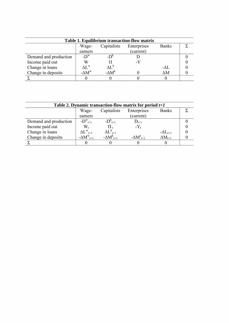
Table 1. Equilibrium transaction-flow matrix Wage-
earners Capitalists Enterprises
(current) Banks Σ
Demand and production -Dw -Dk D 0 Income paid out W Π -Y 0 Change in loans ∆Lw ∆Lk -∆L 0 Change in deposits -∆Mw -∆Mk 0 ∆M 0 Σ 0 0 0 0
Table 2. Dynamic transaction-flow matrix for period t+1 Wage-
earners Capitalists Enterprises
(current) Banks Σ
Demand and production -Dwt+1 -Dk
t+1 Dt+1 0 Income paid out Wt Π t -Yt 0 Change in loans ∆Lw
t+1 ∆Lkt+1 -∆Lt+1 0
Change in deposits -∆Mwt+1 -∆Mk
t+1 -∆Met+1 ∆Mt+1 0
Σ 0 0 0 0
6 The modeling of a monetary macroeconomy
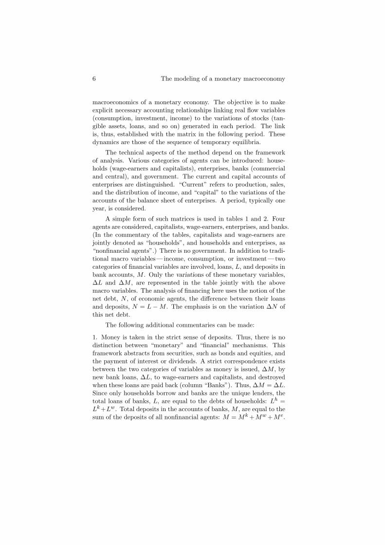
macroeconomics of a monetary economy. The objective is to makeexplicit necessary accounting relationships linking real flow variables(consumption, investment, income) to the variations of stocks (tan-gible assets, loans, and so on) generated in each period. The linkis, thus, established with the matrix in the following period. Thesedynamics are those of the sequence of temporary equilibria.
The technical aspects of the method depend on the frameworkof analysis. Various categories of agents can be introduced: house-holds (wage-earners and capitalists), enterprises, banks (commercialand central), and government. The current and capital accounts ofenterprises are distinguished. “Current” refers to production, sales,and the distribution of income, and “capital” to the variations of theaccounts of the balance sheet of enterprises. A period, typically oneyear, is considered.
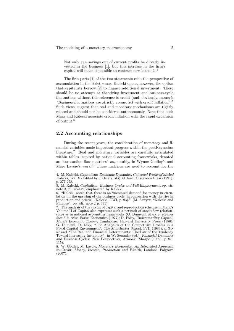
A simple form of such matrices is used in tables 1 and 2. Fouragents are considered, capitalists, wage-earners, enterprises, and banks.(In the commentary of the tables, capitalists and wage-earners arejointly denoted as “households”, and households and enterprises, as“nonfinancial agents”.) There is no government. In addition to tradi-tional macro variables — income, consumption, or investment — twocategories of financial variables are involved, loans, L, and deposits inbank accounts, M . Only the variations of these monetary variables,∆L and ∆M , are represented in the table jointly with the abovemacro variables. The analysis of financing here uses the notion of thenet debt, N , of economic agents, the difference between their loansand deposits, N = L −M . The emphasis is on the variation ∆N ofthis net debt.
The following additional commentaries can be made:
1. Money is taken in the strict sense of deposits. Thus, there is nodistinction between “monetary” and “financial” mechanisms. Thisframework abstracts from securities, such as bonds and equities, andthe payment of interest or dividends. A strict correspondence existsbetween the two categories of variables as money is issued, ∆M , bynew bank loans, ∆L, to wage-earners and capitalists, and destroyedwhen these loans are paid back (column “Banks”). Thus, ∆M = ∆L.Since only households borrow and banks are the unique lenders, thetotal loans of banks, L, are equal to the debts of households: Lh =Lk+Lw. Total deposits in the accounts of banks, M , are equal to thesum of the deposits of all nonfinancial agents: M = Mk +Mw +Me.
The modeling of a monetary macroeconomy 7
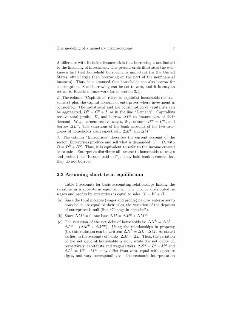
A difference with Kalecki’s framework is that borrowing is not limitedto the financing of investment. The present crisis illustrates the well-known fact that household borrowing is important (in the UnitedStates, often larger than borrowing on the part of the nonfinancialbusiness). Thus, it is assumed that households can also borrow forconsumption. Such borrowing can be set to zero, and it is easy toreturn to Kalecki’s framework (as in section 3.1).
2. The column “Capitalists” refers to capitalist households (as con-sumers) plus the capital account of enterprises where investment isconsidered. The investment and the consumption of capitalists canbe aggregated, Dk = Ck + I, as in the line “Demand”. Capitalistsreceive total profits, Π, and borrow ∆Lk to finance part of theirdemand. Wage-earners receive wages, W , consume Dw = Cw, andborrow ∆Lw. The variations of the bank accounts of the two cate-gories of households are, respectively, ∆Mk and ∆Mw.
3. The column “Enterprises” describes the current account of thesector. Enterprises produce and sell what is demanded: Y = D, withD = Dk +Dw. Thus, it is equivalent to refer to the income createdor to sales. Enterprises distribute all income to households as wagesand profits (line “Income paid out”). They hold bank accounts, butthey do not borrow.
2.3 Assuming short-term equilibrium
Table 1 accounts for basic accounting relationships linking thevariables in a short-term equilibrium. The income distributed aswages and profits by enterprises is equal to sales: Y = W +Π.
(a) Since the total incomes (wages and profits) paid by enterprises tohouseholds are equal to their sales, the variation of the depositsof enterprises is null (line “Change in deposits”).
(b) Since ∆Me = 0, one has: ∆M = ∆Mk + ∆Mw.
(c) The variation of the net debt of households is: ∆Nh = ∆Lk +∆Lw − (∆Mk + ∆Mw). Using the relationships in property(b), this variation can be written: ∆Nh = ∆L−∆M . As statedearlier, in the accounts of banks, ∆M = ∆L. Thus, the variationof the net debt of households is null, while the net debts of,respectively, capitalists and wage-earners, ∆Nk = Lk −Mk and∆Lk = Lw − Mw, may differ from zero, equal with oppositesigns, and vary correspondingly. The economic interpretation
8 The modeling of a monetary macroeconomy
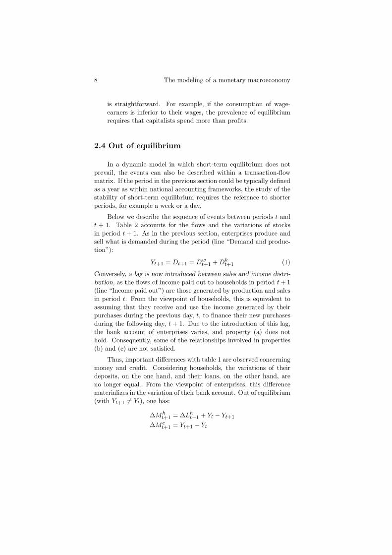
is straightforward. For example, if the consumption of wage-earners is inferior to their wages, the prevalence of equilibriumrequires that capitalists spend more than profits.
2.4 Out of equilibrium
In a dynamic model in which short-term equilibrium does notprevail, the events can also be described within a transaction-flowmatrix. If the period in the previous section could be typically definedas a year as within national accounting frameworks, the study of thestability of short-term equilibrium requires the reference to shorterperiods, for example a week or a day.
Below we describe the sequence of events between periods t andt + 1. Table 2 accounts for the flows and the variations of stocksin period t + 1. As in the previous section, enterprises produce andsell what is demanded during the period (line “Demand and produc-tion”):
Yt+1 = Dt+1 = Dwt+1 +Dkt+1 (1)
Conversely, a lag is now introduced between sales and income distri-
bution, as the flows of income paid out to households in period t+ 1(line “Income paid out”) are those generated by production and salesin period t. From the viewpoint of households, this is equivalent toassuming that they receive and use the income generated by theirpurchases during the previous day, t, to finance their new purchasesduring the following day, t + 1. Due to the introduction of this lag,the bank account of enterprises varies, and property (a) does nothold. Consequently, some of the relationships involved in properties(b) and (c) are not satisfied.
Thus, important differences with table 1 are observed concerningmoney and credit. Considering households, the variations of theirdeposits, on the one hand, and their loans, on the other hand, areno longer equal. From the viewpoint of enterprises, this differencematerializes in the variation of their bank account. Out of equilibrium(with Yt+1 6= Yt), one has:
∆Mht+1 = ∆Lht+1 + Yt − Yt+1
∆Met+1 = Yt+1 − Yt
The modeling of a monetary macroeconomy 9
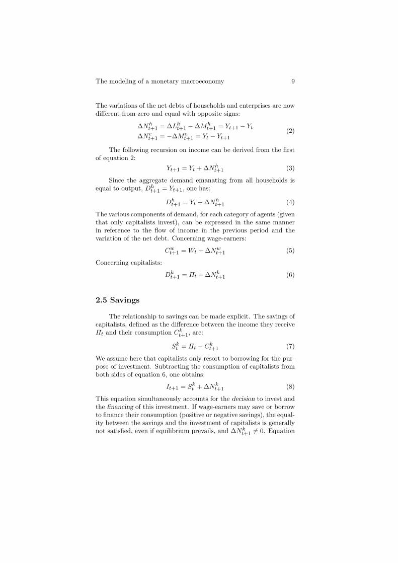
The variations of the net debts of households and enterprises are nowdifferent from zero and equal with opposite signs:
∆Nht+1 = ∆Lht+1 −∆Mh
t+1 = Yt+1 − Yt∆Ne
t+1 = −∆Met+1 = Yt − Yt+1
(2)
The following recursion on income can be derived from the firstof equation 2:
Yt+1 = Yt + ∆Nht+1 (3)
Since the aggregate demand emanating from all households isequal to output, Dht+1 = Yt+1, one has:
Dht+1 = Yt + ∆Nht+1 (4)
The various components of demand, for each category of agents (giventhat only capitalists invest), can be expressed in the same mannerin reference to the flow of income in the previous period and thevariation of the net debt. Concerning wage-earners:
Cwt+1 = Wt + ∆Nwt+1 (5)
Concerning capitalists:
Dkt+1 = Πt + ∆Nkt+1 (6)
2.5 Savings
The relationship to savings can be made explicit. The savings ofcapitalists, defined as the difference between the income they receiveΠt and their consumption Ckt+1, are:
Skt = Πt − Ckt+1 (7)
We assume here that capitalists only resort to borrowing for the pur-pose of investment. Subtracting the consumption of capitalists fromboth sides of equation 6, one obtains:
It+1 = Skt + ∆Nkt+1 (8)
This equation simultaneously accounts for the decision to invest andthe financing of this investment. If wage-earners may save or borrowto finance their consumption (positive or negative savings), the equal-ity between the savings and the investment of capitalists is generallynot satisfied, even if equilibrium prevails, and ∆Nk
t+1 6= 0. Equation
10 The modeling of a monetary macroeconomy
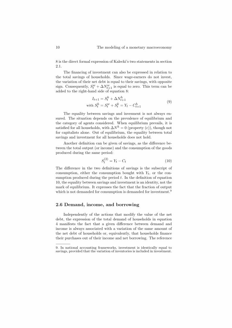
8 is the direct formal expression of Kalecki’s two statements in section2.1.
The financing of investment can also be expressed in relation tothe total savings of households. Since wage-earners do not invest,the variation of their net debt is equal to their savings, with oppositesign. Consequently, Swt + ∆Nw
t+1 is equal to zero. This term can beadded to the right-hand side of equation 8:
It+1 = Sht + ∆Nht+1
with Sht = Swt + Skt = Yt − Cht+1
(9)
The equality between savings and invesment is not always en-sured. The situation depends on the prevalence of equilibrium andthe category of agents considered. When equilibrium prevails, it issatisfied for all households, with ∆Nh = 0 (property (c)), though notfor capitalists alone. Out of equilibrium, the equality between totalsavings and investment for all households does not hold.
Another definition can be given of savings, as the difference be-tween the total output (or income) and the consumption of the goodsproduced during the same period:
S(2)t = Yt − Ct (10)
The difference in the two definitions of savings is the subscript ofconsumption, either the consumption bought with Yt, or the con-sumption produced during the period t. In the definition of equation10, the equality between savings and investment is an identity, not themark of equilibrium. It expresses the fact that the fraction of outputwhich is not demanded for consumption is demanded for investment.9
2.6 Demand, income, and borrowing
Independently of the actions that modify the value of the netdebt, the expression of the total demand of households in equation4 manifests the fact that a given difference between demand andincome is always associated with a variation of the same amount ofthe net debt of households or, equivalently, that households financetheir purchases out of their income and net borrowing. The reference
9. In national accounting frameworks, investment is identically equal tosavings, provided that the variation of inventories is included in investment.
The modeling of a monetary macroeconomy 11
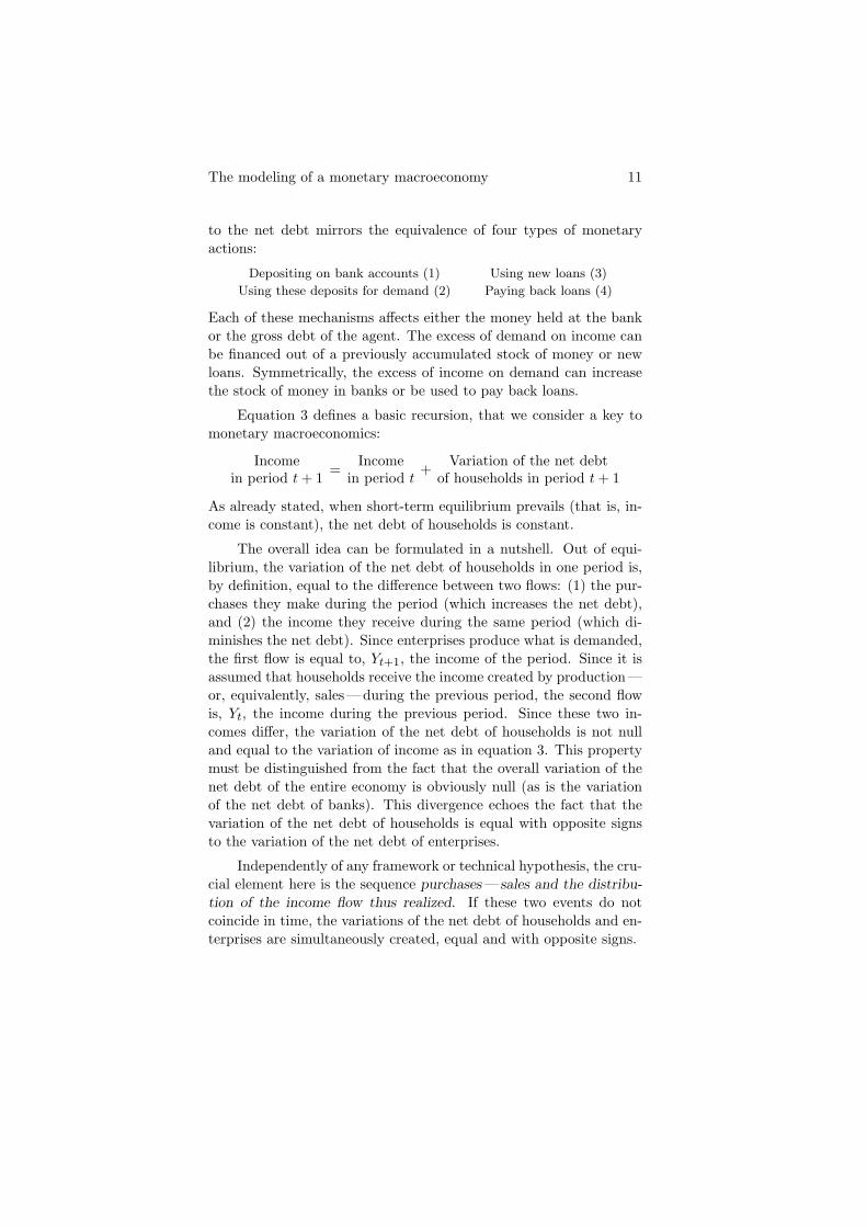
to the net debt mirrors the equivalence of four types of monetaryactions:
Depositing on bank accounts (1)
Using these deposits for demand (2)
Using new loans (3)
Paying back loans (4)
Each of these mechanisms affects either the money held at the bankor the gross debt of the agent. The excess of demand on income canbe financed out of a previously accumulated stock of money or newloans. Symmetrically, the excess of income on demand can increasethe stock of money in banks or be used to pay back loans.
Equation 3 defines a basic recursion, that we consider a key tomonetary macroeconomics:
Incomein period t+ 1 = Income
in period t+ Variation of the net debt
of households in period t+ 1
As already stated, when short-term equilibrium prevails (that is, in-come is constant), the net debt of households is constant.
The overall idea can be formulated in a nutshell. Out of equi-librium, the variation of the net debt of households in one period is,by definition, equal to the difference between two flows: (1) the pur-chases they make during the period (which increases the net debt),and (2) the income they receive during the same period (which di-minishes the net debt). Since enterprises produce what is demanded,the first flow is equal to, Yt+1, the income of the period. Since it isassumed that households receive the income created by production —or, equivalently, sales — during the previous period, the second flowis, Yt, the income during the previous period. Since these two in-comes differ, the variation of the net debt of households is not nulland equal to the variation of income as in equation 3. This propertymust be distinguished from the fact that the overall variation of thenet debt of the entire economy is obviously null (as is the variationof the net debt of banks). This divergence echoes the fact that thevariation of the net debt of households is equal with opposite signsto the variation of the net debt of enterprises.
Independently of any framework or technical hypothesis, the cru-cial element here is the sequence purchases — sales and the distribu-
tion of the income flow thus realized. If these two events do notcoincide in time, the variations of the net debt of households and en-terprises are simultaneously created, equal and with opposite signs.
12 The modeling of a monetary macroeconomy
3 - Money, credit, and (in)stability
This section is devoted to the (in)stability of short-term equi-librium. In a dynamic model, stability is typically subject to condi-tions. Within (post)Keynesian models, the condition for the stabilityof short-term equilibrium (denoted as “Keynesian stability”), is thatthe slope of the investment function must be smaller than the slopeof the saving function. It is generally assumed that this condition issatisfied.
The first section below expresses such conditions within two sim-ple variants of Kalecki’s models, in which monetary relationships arelimited to the borrowing of capitalists to finance investment as in sec-tions 2.1 and 2.5. We contend that, in the absence of the stabilizingaction of the central bank, the capitalist macroeconomy would alwaysbe unstable, what we denote as “built-in instability”. Consequently,the action of the central bank must be treated as a basic componentof macro theory, and not an optional sophistication of mechanismsotherwise defined. This is the object of the second section.
A preliminary statement must be made concerning the decisionto produce by enterprises. In a dynamic model built to study thestability of short-term equilibrium, two alternative hypotheses canbe made: (1) Enterprises produce exactly what is demanded; or (2)Demand is not yet known when enterprises decide on output, andinventories of unsold goods can exist or rationing prevail.10 In thepresent study, we use the first option, in conformity with the vastmajority of (post)Keynesian models.
3.1 Built-in instability
Kalecki’s framework is well known. Two agents are considered:(1) wage-earners who have no access to credit and consume exactlywhat is allowed by their wages; and (2) capitalists who have accessto credit and consume a given fraction, 1 − s, of profits, and may
10. This is our favorite framework. The accounting is, however, more com-plex, as inventories of unsold commodities must be financed. G. Dumenil,D. Levy, The Economics of the Profit Rate: Competition, Crises, and His-torical Tendencies in Capitalism, Aldershot: Edward Elgar (1993); and Ladynamique du capital. Un siecle d’economie americaine, Paris: PressesUniversitaires de France (1996).
The modeling of a monetary macroeconomy 13
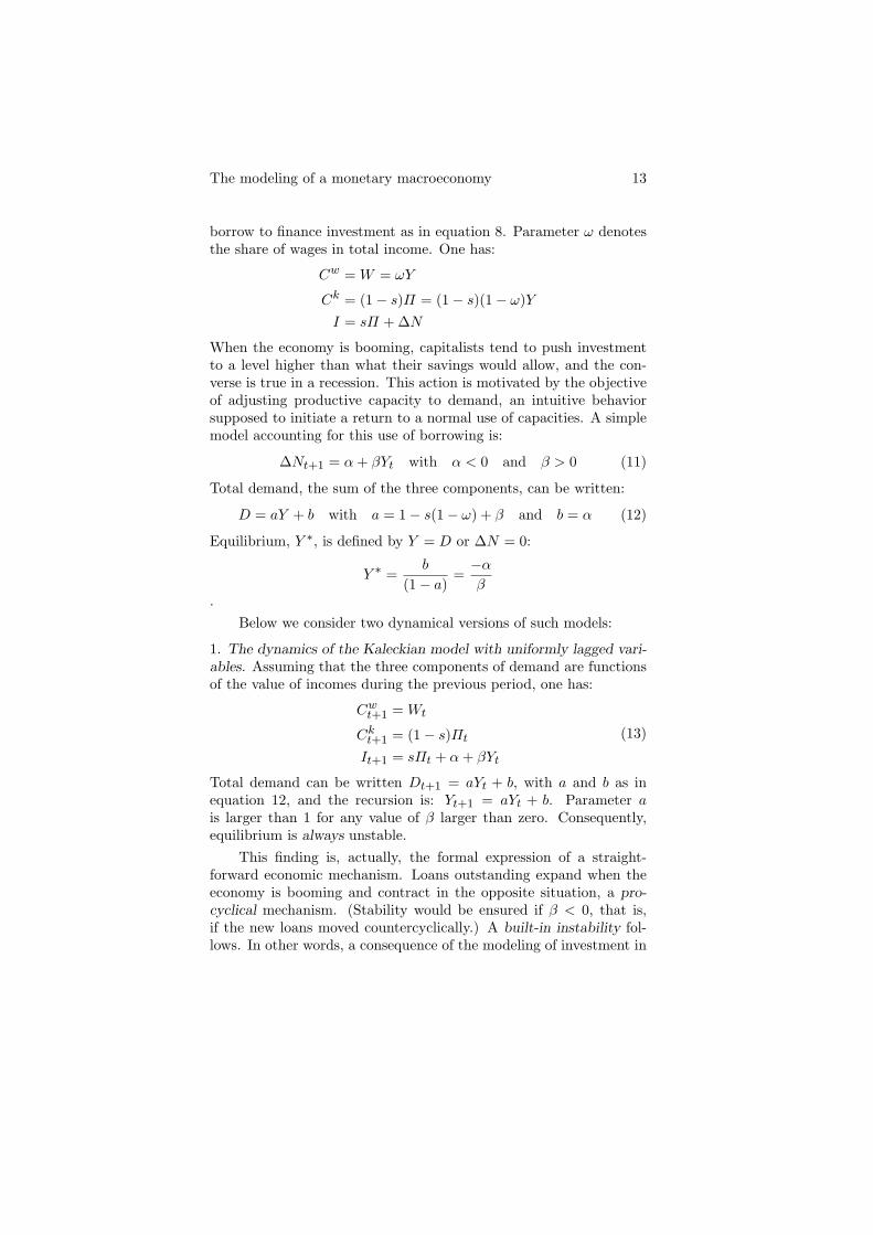
borrow to finance investment as in equation 8. Parameter ω denotesthe share of wages in total income. One has:
Cw = W = ωY
Ck = (1− s)Π = (1− s)(1− ω)YI = sΠ + ∆N
When the economy is booming, capitalists tend to push investmentto a level higher than what their savings would allow, and the con-verse is true in a recession. This action is motivated by the objectiveof adjusting productive capacity to demand, an intuitive behaviorsupposed to initiate a return to a normal use of capacities. A simplemodel accounting for this use of borrowing is:
∆Nt+1 = α+ βYt with α < 0 and β > 0 (11)
Total demand, the sum of the three components, can be written:
D = aY + b with a = 1− s(1− ω) + β and b = α (12)
Equilibrium, Y ∗, is defined by Y = D or ∆N = 0:
Y ∗ =b
(1− a)=−αβ
.Below we consider two dynamical versions of such models:
1. The dynamics of the Kaleckian model with uniformly lagged vari-ables. Assuming that the three components of demand are functionsof the value of incomes during the previous period, one has:
Cwt+1 = Wt
Ckt+1 = (1− s)ΠtIt+1 = sΠt + α+ βYt
(13)
Total demand can be written Dt+1 = aYt + b, with a and b as inequation 12, and the recursion is: Yt+1 = aYt + b. Parameter ais larger than 1 for any value of β larger than zero. Consequently,equilibrium is always unstable.
This finding is, actually, the formal expression of a straight-forward economic mechanism. Loans outstanding expand when theeconomy is booming and contract in the opposite situation, a pro-cyclical mechanism. (Stability would be ensured if β < 0, that is,if the new loans moved countercyclically.) A built-in instability fol-lows. In other words, a consequence of the modeling of investment in
14 The modeling of a monetary macroeconomy
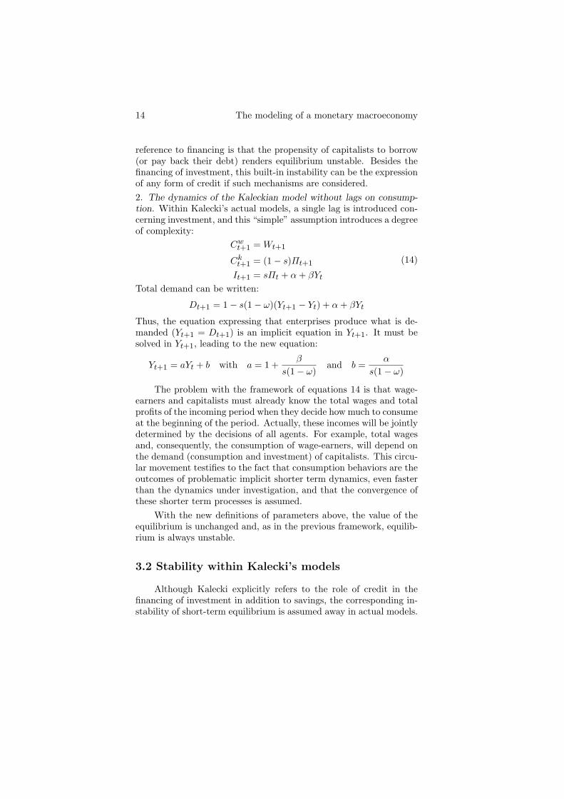
reference to financing is that the propensity of capitalists to borrow(or pay back their debt) renders equilibrium unstable. Besides thefinancing of investment, this built-in instability can be the expressionof any form of credit if such mechanisms are considered.2. The dynamics of the Kaleckian model without lags on consump-tion. Within Kalecki’s actual models, a single lag is introduced con-cerning investment, and this “simple” assumption introduces a degreeof complexity:
Cwt+1 = Wt+1
Ckt+1 = (1− s)Πt+1
It+1 = sΠt + α+ βYt
(14)
Total demand can be written:
Dt+1 = 1− s(1− ω)(Yt+1 − Yt) + α+ βYt
Thus, the equation expressing that enterprises produce what is de-manded (Yt+1 = Dt+1) is an implicit equation in Yt+1. It must besolved in Yt+1, leading to the new equation:
Yt+1 = aYt + b with a = 1 +β
s(1− ω)and b =
α
s(1− ω)
The problem with the framework of equations 14 is that wage-earners and capitalists must already know the total wages and totalprofits of the incoming period when they decide how much to consumeat the beginning of the period. Actually, these incomes will be jointlydetermined by the decisions of all agents. For example, total wagesand, consequently, the consumption of wage-earners, will depend onthe demand (consumption and investment) of capitalists. This circu-lar movement testifies to the fact that consumption behaviors are theoutcomes of problematic implicit shorter term dynamics, even fasterthan the dynamics under investigation, and that the convergence ofthese shorter term processes is assumed.
With the new definitions of parameters above, the value of theequilibrium is unchanged and, as in the previous framework, equilib-rium is always unstable.
3.2 Stability within Kalecki’s models
Although Kalecki explicitly refers to the role of credit in thefinancing of investment in addition to savings, the corresponding in-stability of short-term equilibrium is assumed away in actual models.
The modeling of a monetary macroeconomy 15
In some instances11, Kalecki uses a variant of the accelerator model.In other contexts12, investment beyond savings is linked to a discrep-ancy between an investment that would have yielded a “normal profitrate”, and the actual investment in the previous period, in a mannerensuring stability:
The considerations concerning the prerequisites for reinvest-ment of entrepreneurial savings — i.e., whether the invest-ment decisions taken in a given year are to be equal to en-trepreneurial savings, exceed them or fall short of them —are closely related to the idea of the “normal rate of profit”π on a new investment.13
A last option is the assumption that capitalists only invest a fractionof their savings.14 None of these ways out are really convincing.
3.3 Stabilizing a monetary economy
The importance of the finding concerning a built-in instability ina monetary macroeconomy must be stressed. This property is, how-ever, subject to the assumption that capitalists autonomously decideon borrowing or, equivalently, that the financial system accommo-dates their demand. A consequence is that a countercyclical action ofcentral institutions is a requirement. This action must be understoodas a “structural” component of capitalism, as soon (and inasmuch)as monetary mechanisms reach an advanced degree of development.This analysis obviously confers a crucial role on the action of centralmonetary institutions, first of all, the central bank, but also poten-tially more complex institutions, such as agencies, within a broadlydefined regulatory framework. Demand policies by governments arealso involved. It is only for simplicity that, with little exception, theremainder of this study refers to the “central bank” and monetarypolicy.
This statement concerning macrodynamics in capitalism has cru-cial theoretical implications. The mechanisms implied in the stabi-lizing role of central monetary authorities are a necessary component
11. M. Kalecki, Theory of Economic Dynamics. An Essay on Cyclical andLong-Run Changes in Capitalist Economy, New York: Monthly ReviewPress (2009), ch. 9, p. 102.12. M. Kalecki, “Trend and Business Cycles Reconsidered”, Economic Jour-nal, 78 (1968), p. 263-276, p. 268.13. M. Kalecki, Theory of Economic Dynamics, op. cit. note 11, p. 98.14. M. Kalecki, ibid., p. 98.
16 The modeling of a monetary macroeconomy
of the theory of the macroeconomy, not sophistications that can beadded or not, once the fundamental framework has been devised.
The consideration of the stabilizing behavior of the central bankdoes not imply, however, that the stability of short-term equilib-rium is permanently ensured. First, considering the financial systemglobally — commercial banks and the central bank — the outcome isuncertain. The action of the financial system may accompany andstimulate phases of expansion, accommodating or contributing to thebuilt-in instability. Second, stability conditions also depend on thebehaviors of nonfinancial agents, and these behaviors are also subjectto nonfinancial determinants, notably the profitability of capital andthe capacity utilization rate.
Thus, the countercyclical action of the central bank or the gov-ernment only places limits on the vagaries of the macroeconomy butdoes not eliminate business-cycle fluctuations. In the absence of suchmechanisms, the economy would, however, be fundamentally unsta-ble. The course of output along the phases of the business cyclesuggests that this management of the macroeconomy is only par-tially successful. Stability may be ensured “to some extent” duringspecific periods and, recurrently, instability prevails during other pe-riods. Overheatings and recessions are always around the corner.
The requirement of a central management of the macroeconomyis a crucial aspect of Keynes’ assessment of capitalism. It is alsopresent in Kalecki’s work, and is an important theme within thepostKeynesian school. One limitation of the Keynesian perspectiveis, however, that macro polices are considered in reference to thenecessity of adjusting the level of equilibrium to appropriate values,not as responding to the requirement of the preservation of stability.
4 - The principle of co-determination
One thing is sure, monetary mechanisms should not be mod-eled in the traditional framework of the confrontation between givensupply and demand curves. Money and credit are not goods orservices produced by financial enterprises and demanded by nonfi-nancial agents. The section introduces the alternative principle of“co-determination”. Besides the overall idea that real and monetary
The modeling of a monetary macroeconomy 17
variables are simultaneously determined, the notion emphasizes thatthis determination results from the joint behavior of nonfinancial andfinancial agents.
The relationship between real and monetary variables, as in thefirst facet of co-determination above, is already a central aspect ofthe analysis in the previous sections. Concerning the second facet,familiar processes of interaction are involved. For example, a house-hold willing to buy a house goes to the bank and adjusts its ambitionsto its capability to borrow in a reciprocal process of negotiation andassessment of the costs and risks of borrowing and lending.
We call the “co-determined monetary function”, the single func-tions in which these simultaneous and joint determinations are ex-pressed. For example, the behavior of the banking system is in-troduced into the equations accounting for the determination of thedemand of households. The same is true if the entire macroeconomyis considered.
4.1 Nonfinancial and financial agents
The thesis of a built-in instability in capitalism in section 3.1clearly sets out the two aspects of monetary mechanisms. Monetarymechanisms allow for the expansion of demand beyond available in-come when the economy is booming (or the contraction of demandbelow income when the economy is depressed), and this procyclical(thus, destabilizing) mechanism makes of the stabilizing action of thecentral bank a basic requirement.
Abstracting from government deficits or surpluses to which sec-tion 5.4 is devoted, the dynamics governing the complex issuance/de-struction of money, lending/borrowing, and deposits/withdrawals are,actually, the combined outcome of the actions of three categories ofagents: (1) households, (2) commercial banks seeking profits, and (3)the central bank in charge of the management of the macroeconomyand the stability of the financial system:
1. Households simultaneously consider their eagerness to buy, theirincome, the cost of borrowing, and their monetary situation.2. Commercial banks seek maximum profits, given the assessment ofcorresponding risks. Depending on the situation of potential borrow-ers, they may accept or deny loans, and they can impact the amounts.They take into consideration their own situation, including their ca-pability to access available and cheap financing on the part of other
18 The modeling of a monetary macroeconomy
banks and the central bank. Obviously, they must abide by a numberof regulations, which differ significantly among countries and periods,constraining their action to distinct degrees.3. The central bank acts with the triple objective of supporting theaction of banks, managing the macroeconomy, and ensuring the sta-bility of the financial system. This means taming or stimulating eco-nomic activity, as well as maintaining the stability of the general pricelevel and the levels of indebtedness, with important consequences onthe capability of individual agents and commercial banks to borrow.In the accomplishment of these functions, the central bank is sur-rounded by a number of agencies. Besides interest rates, variousratios (concerning reserves or banks’ equity), and a wealth of regu-lations perform the task. The frontier between central control andprivate initiative is susceptible of important variation as manifest inthe current crisis.
These three categories of agents constantly interact and negotiate.Monetary mechanisms are determined as the collective and conflictingoutcomes of such behaviors and mechanisms.
Concerning the relationship with postKeynesian economists, thereis a common agreement concerning the initial statement that, inthe modeling of monetary variables, the confrontation between sup-ply and demand functions whose intersection defines an equilibriumprice (the interest rate) is inappropriate.15 But the emphasis withinpostKeynesian economics is exclusively on the behavior of nonfinan-cial agents, modeled in demand functions for money and loans. Thesupply behavior of the banking system is supposed to accommodatethis demand (for any value of the interest rate).16
4.2 The co-determined monetary function
The joint determination of real and monetary variables refers toa whole set of variables such as purchases, new loans, the amount ofdebt paid back, and the changes in the bank accounts. One optionwould be to model separately these various elements. We consider,however, that the demand or variation of the net debt can be syn-thetically described in single functions for a given agent, a group
15. This criticism also applies to Keynes’ analysis of the determination ofinterest rates.16. For example, the financial system “has no choice but to accommodate”(B.J. Moore, “The Endogenous Money Stock”, Journal of Post KeynesianEconomics, 2 (1979), p. 49-70, p. 58).
The modeling of a monetary macroeconomy 19
of agents, or the entire macroeconomy, depending on the frameworkunder investigation. The consideration of single functions echoes theview that the central bank has a capability to affect the outcome ofthe complex set of monetary mechanisms impacting the determina-tion of demand.
The synthetic expression of such mechanisms in a single func-tion allows for the construction of macro models that can be treatedanalytically, as in section 5. In our opinion, such models account forthe main properties of a macroeconomy with money.
Equations 4, 5, or 8 are accounting relationships linking the de-mands and variations of the net debts for, respectively, the entiremacroeconomy, wage-earners, and capitalists. They show that, giventhe income resulting from the sales during the previous period, itis equivalent to determine one of the two variables. We choose tomodel the variation of the net debts, and denote the correspondingfunctions as the “co-determined monetary functions”, F :
∆N = F
To the co-determined monetary functions of each individual or col-lective agent corresponds a demand function and reciprocally. In thesimplest option of a single function for the entire macroeconomy, themodel for demand is:
Dt+1 = Yt + Ft+1 (15)
An example of such a co-determined monetary function is:
F = α+ βY − γN − δj (16)
Besides the constant α, three linear terms are involved:
1. βY . This first term accounts for the procyclical components ofthe dynamics of demand and borrowing: (1) the propensity of non-financial agents to borrow; (2) the propensity of commercial banksto accommodate the demands for credit on the part of nonfinancialagents when the economy is booming (or to stimulate such demandsas in the mortgage wave in the United States after 2000); (3) theaccommodative behavior of the central bank during phases of expan-sion. There is a symmetrical aspect to each of these componentsas, during phases of contraction of output, households refrain fromborrowing.
To this procyclical component, one must add one or several termsaccounting for the limitations placed on borrowing (their stimulation
20 The modeling of a monetary macroeconomy
in symmetrical situations) due to the deviation of a number of vari-ables that might threaten individual or collective interests. Two suchterms are considered in equation 16:2. −γN . This term accounts for a first group of countercyclicalbehaviors: (1) Commercial banks are watchful of the levels of in-debtedness, N , of their customers; (2) Central banks are also con-cerned by rising indebtedness, which may jeopardize the stability ofthe macroeconomy or of the financial system.3. −δj. Central banks are wary of inflation rates, j, and tend tostrengthen monetary policy during phases of inflation. Assumingthat overheating is associated with increased inflation rates, and con-versely for recessions, this behavior has a countercyclical impact onthe macroeconomy.
Various facets of the above reactions lead to the modification ofinterest rates on the part of the central bank (and commercial banks).An option is, thus, to include the interest rate into the co-determinedmonetary function. A larger value of the interest rate can be expectedto have the following effects: (1) diminished borrowings; (2) earlyamortization; (3) increased deposits; or (4) diminished withdrawals.In all instances, F is reduced if i is larger.
Ft+1 = α+ βYt − ϕit (17)
Then, a reaction function must be introduced modeling the manipu-lation of interest rate, assuming that i is altered procyclically by thecentral bank with the objective of stabilizing the macroeconomy.
Obviously, these terms must be understood as simple particu-lar forms of more general mechanisms. The central element here isthe combination of pro-, βY , and countercyclical mechanisms, −γN ,−δj, and −ϕi.
5 - Checking built-in instability
This section introduces various models of a monetary macroe-conomy based on the principle of co-determination as defined in theprevious section. Thus, underlying each of these models is a recursionsuch as in equation 3:
Yt+1 = Yt + Ft+1
The modeling of a monetary macroeconomy 21
The general framework is simple. There is no growth, as invest-ment is only a component of demand. No difference is made betweenwage-earners and capitalists, and demand is considered globally, ab-stracting from possible specific behaviors relative to consumption andinvestment. In the model of section 5.4 demand also originates fromthe goverment. Thus, it is the only model in which two co-determinedmonetary functions are introduced instead of one.
Pro- and countercyclical mechanisms are combined. Two firstvariants are considered depending on the behavior of the bankingsystem: (1) The banking system reacts negatively to the levels of thenet debt; (2) The central bank responds to inflation. Two additionalmodels are introduced concerning, respectively, stabilizing policiesin which the interest rate is increased when output rises, and fiscalpolicy responding countercyclically to the levels of output.
Recursions with one or two variables are obtained, and the equi-librium values of the variables can be determined. The stability ofequilibrium is ensured in each model under the intuitive conditionthat the countercyclical mechanisms dominate.
5.1 Controlling indebtedness
Besides a constant, two terms are considered in the macro co-determined monetary function:
Ft+1 = α+ βYt − γNtA procyclical term, βYt, models the joint behavior of nonfinancialagents and commercial banks. A countercyclical term, −γNt, modelsthe action of the banking system. The consideration of the levels ofindebtedness by commercial banks is an aspect of their managementof risks. The same is true of the central bank, but the objective is thepreservation of the stability of the overall banking system to preventfinancial crises.
With Ft+1 as above, the corresponding recursion with two vari-ables is:
Yt+1 = Yt + Ft+1
Nt+1 = Nt + Ft+1
This recursion can be broken down into two autonomous components,substituting Z1 and Z2 for Y and N , with Z1 = Y − N and Z2 =
22 The modeling of a monetary macroeconomy
βY − γN :Z1t+1 = Z1
t
Z2t+1 = (1 + β − γ)Z2
t + α(β − γ)The short-term equilibrium is:
Z1∗ = Z10 and Z2∗ = −α
Returning to the original variables, Y and N :
Y ∗ =α+ γ(Y0 −N0)
γ − β and N∗ =α+ β(Y0 −N0)
γ − βThese equilibrium values depend on all parameters, α, β and γ, andon the initial values, Y0 and N0, of the two variables.
The stability of the equilibrium in Z2 is subject to the condition:
1 + β − γ < 1, that is, γ > β
Parameter γ measures the intensity of the countercyclical componentin the action of the banking system, and β, the procyclical compo-nent. Stability is ensured if the countercyclical component prevails.(The contemporary crisis provides an interesting illustration of theconsequences of the excessive relaxation of the countercyclical com-ponent.17)
5.2 Targeting price stability
This section introduces an alternative model of the macro co-determined monetary function in which countercyclical proceduresare fully in the hands of the central bank, while the procyclical termcan be imputed to all other agents. The objective of the centralbank is price stability. In this framework, it is obviously necessary toaccount for the dynamics of the determination of prices by enterprises.
The rigidity of prices is a basic assumption in the Keynesianperspective. The adjustment between supply and demand is madeby quantities — that is, enterprises set output to the level of demand,with rigid prices — not by prices as in a neoclassical model. We arein full agreement with this viewpoint, but we believe it must be in-terpreted as an approximation. Instead of “rigid”, prices should besaid to be “sticky”, meaning “slowly adjusted” — adjusted much lessrapidly than outputs.
17. G. Dumenil, D. Levy, The Crisis of Neoliberalism, Harvard: HarvardUniversity Press (2011).
The modeling of a monetary macroeconomy 23
Enterprises mark up on costs, pt = µtw, where the nominal wagerate, w, is the only cost and is constant. Enterprises slowly adjustthe mark-up rate µt. A simple option is to consider that enterprisesincrease their mark-up rate when output is larger than its targetvalue, Y , and conversely if output is lower than this target:
µt+1 = µt(1 + ε(Yt − Y )
)
Thus, the inflation rate is proportional to the deviation of output:
jt =pt+1 − pt
pt=µt+1 − µt
µt= ε(Yt − Y )
The macro co-determined monetary function combines two com-ponents, a procyclical term, βYt, and a countercyclical term −δjt(and a constant α):
Ft+1 = α+ βYt − δjt = α+ εδY + (β − εδ)Yt (18)
The recursion, with only one variable, is:
Yt+1 = aYt + b with a = 1 + β − εδ and b = α+ εδY
Short-term equilibrium prevails when:
Y ∗ =b
1− a, j∗ = ε(Y ∗ − Y ), and F ∗ = 0
The position of the equilibrium depends on the values of all parame-ters, but not on the initial values of the variables. The inflation rateis constant but not null, except if Y ∗ = Y .
The condition for stability, a < 1, is:
εδ > β
The first term, εδ, measures the strength of the countercyclical com-ponent. It is the product of ε, the degree of the reaction of enterprisesto the disequilibrium concerning the level of production, and δ, thedegree of the reaction of the central bank to inflation. The formeris assumed to be weak. Thus, δ must be strong enough to ensurethat the countercyclical component εδ dominates over the procyclicalcomponent β. In this framework, as in the model in the previous sec-tion, the central bank has a capability to stabilize the macroeconomy,but this capability is subject to conditions in which the behaviors ofnonfinancial and financial agents are jointly involved.
24 The modeling of a monetary macroeconomy
5.3 Manipulating interest rates
The manipulation of the interest rate of the central bank is animportant tool in the conduct of monetary policy. The central bankadjusts i depending on various targets such as inflation or indebt-edness. The form of the macro co-determined demand function isthe one introduced in equation 17. A simple model of the stabiliz-ing action of the central bank is that it increases the interest ratewhen output rises, and conversely when output diminishes, that is,the interest rate is altered countercyclically. The reaction functionis:
it+1 = it + ν(Yt+1 − Yt) (19)
The recursion is:
Yt+1 = α+ (1 + β)Yt − ϕitit+1 = it + ν(Yt+1 − Yt)
It can be shown that the equilibrium is stable if the reaction of thecentral bank, measured by parameter ν, is strong enough. In theabsence of the dynamics of the interest rate, the equilibrium wouldbe unstable.
5.4 Fiscal policy
There are two aspects to fiscal policy. It can be the mere effect ofthe stickiness of expenses compared to the variations of the revenueof the government, or a deliberate action intending to stimulate themacroeconomy.
A difference with the two previous models is that demand em-anates from two categories of agents, government and households.Two co-determined monetary functions, FG and Fh, are correspond-ingly considered. We assume that the sources of government revenueare taxes paid by nonfinancial agents, proportional to aggregate in-come: τY . Government expenses (the purchase of goods and services)move countercyclically: larger than government revenue during reces-sions (Yt < Y ), and lower, during periods of high activity (Yt > Y ).Thus, the government borrows during periods of recession and paysback its debt during periods of high activity. Its net debt variescountercyclically:
FG = −βG(Yt − Y )
The modeling of a monetary macroeconomy 25
The disposable income of households is (1 − τ)Yt. Their monetarybehavior is procyclical, and their co-determined monetary functionis:
Fh = α+ βYt
Equilibrium is stable if the countercyclical effect of fiscal policy isstrong enough.
6 - Business-cycle fluctuations
This section is devoted to the analysis of business-cycle fluc-tuations. Section 6.1 concludes concerning our own interpretation.Section 6.2 briefly retakes the issue in Kalecki’s work and within the(post)Keynesian perspective. Section 6.3 discusses Minsky’s frame-work of “financial instability”.
6.1 The (in)stability of short-term equilibriumcentral stage
The main thesis in the present study is the economic relevanceof the (in)stability issue in the analysis of business-cycle fluctuations.Three main aspects must be emphasized:
1. The conditions for the stability of short-term equilibrium may bemet or not, and the identification of phases in which stability andinstability alternatively prevail is a distinction of crucial importance.2. The thesis in section 3.1 of a built-in instability in capitalismascribes this tendency to monetary mechanisms: (1) the effect of apropensity on the part of nonfinancial agents to spend more than isallowed by previously garnered incomes (or symmetrically, to contracttheir spendings below what income flows would allow, that is, todiminish their net debt); and (2) the tendency of financial institutionsto accommodate these demands.3. This built-in instability renders necessary the stabilizing action ofthe central bank. Periods of instability manifest the recurrent failuresof central institutions to check this built-in instability.
This emphasis on stability conditions opens a new field in whichthe economic interpretation of these conditions becomes a central
26 The modeling of a monetary macroeconomy
element in the analysis of the business cycle. The ambition of sections4 and 5 is to provide the foundations of a theory of stability conditionssusceptible of empirical application. Parameters such as β, γ, orδ, are not simple technical instruments. Their possible variationsare subject to economic interpretation. The reference to a “cycle”suggests cyclical patterns of variations of these coefficients, but more“structural” variations can also alter the forms of the business cycle.Various examples could be given of such transformations. The suddenchange in the conduct of monetary policy — the 1979 coup18 — thatmarked the entrance into neoliberalism in the United States meant arise of δ; the transformation of financial mechanisms that led to thesubprime crisis can be interpreted as a decline of γ.
Many basic aspects of the business cycle can be investigatedwithin linear frameworks, as in the present study. But the explana-tory power of linear models cannot be extended to the vagaries ofthe macroeconomy at a significant distance from equilibrium. Oncethe possible instability of short-term equilibrium is acknowledged, itbecomes necessary to consider nonlinear dynamic models.
In the 1980s, in an attempt to account for such dynamics, webuilt nonlinear dynamic models with a “pitchfork singularity”, inwhich the (in)stability of short-term equilibrium is central.19 Thesemodels account for: (1) the gradual drift toward situations in whichthe short-term equilibrium is unstable; and (2) the sudden fall down-ward.
The succession of such phases to the point of instability echoesthe description of the cycle of industry by Marx:
The path characteristically described by modern industry,which takes the form of a decennial cycle (interrupted bysmaller oscillations) of periods of average activity, produc-tion at high pressure, crisis, and stagnation [...].20
18. G. Dumenil, D. Levy, Capital Resurgent. Roots of the NeoliberalRevolution, Harvard: Harvard University Press (2004).19. G. Dumenil, D. Levy, “The Macroeconomics of Disequilibrium”, Jour-nal of Economic Behavior and Organization, 8 (1987), p. 377-395; “MicroAdjustment Behavior and Macro Stability”, Seoul Journal of Economics, 2(1989), p. 1-37; and “The Real and Financial Determinants”, op. cit. note7.20. K. Marx, Capital, Volume III (1894), New York: First Vintage BookEdition (1981), p. 785.
The modeling of a monetary macroeconomy 27
6.2 Kalecki’s and (post)Keynesian interpretations
As already contended, the focus of traditional Keynesian eco-nomics is more on the position of equilibrium than on the fluctuationsproper of the general level of activity. The same is true of postKey-nesian frameworks where the investigation is extended to long-termsteady states. Although the contrast is sharp between these ap-proaches and ours, it is important to stress that, in our opinion, theemphasis on the (in)stability of short-term equilibrium does not pre-clude the relevance of the degree to which productive capacities areused. In other works, we considered dynamic frameworks account-ing for the shift of the position of equilibrium in the longer run.21
This is the “postKeynesian component” of our analysis. Monetarymechanisms are also central stage.
To the contrary, the final objective of Kalecki’s investigation isexplicitly the business cycle. The cycle is interpreted as the mani-festation of recurrent shocks on a macroeconomy in the vicinity ofa stable short-term equilibrium. After a shock, output tends to re-converge toward equilibrium, but a new shock occurs, and so on,creating permanent oscillations. This emphasis on the dynamics ofthe macroeconomy around short-term equilibrium defines a commonpoint with Kalecki’s approach, although Kalecki does not considerthe succession of periods of stability and instability.
The (in)stability issue is not completely absent, however, fromthe traditional Keynesian perspective. It is (or was) discussed inthe framework of “Keynesian stability”, but only the case in whichstability is ensured is considered relevant.22
Besides Minsky, to which the following section is devoted, NicholasKaldor stands out as an exception in this regard. In his paper on thetrade cycle23, Kaldor contends that, in a vicinity of a normal use ofproductive capacities, the slope of the investment function is largerthan the slope of the saving function or, equivalently, that the slopeof the aggregate demand function is larger than 1. Consequently,
21. G. Dumenil, D. Levy, “Being Keynesian in the Short Term”, op. cit.note 1.22. There is some interest in the instability of long-term equilibrium, de-noted as “Harrodian instability” (P. Skott, Growth, Instability and Cycles:Harrodian and Kaleckian Models of Accumulation and Income Distribu-tion, University of Massachusetts, Amherst, Economics Department Work-ing Paper Series (2008)).23. N. Kaldor, “A Model of the Trade Cycle”, Economic Journal, 50 (1940),p. 781-92.
28 The modeling of a monetary macroeconomy
the instability of the short-term equilibrium is viewed as a centralcomponent of the analysis of the business cycle.24
6.3 Minsky’s financial instability
Because of the importance conferred on instability and the ref-erence to monetary mechanisms, a link can be established betweenthe perspective in the present study and Minsky’s theory of financialinstability. The central character of instability is clearly set out byMinsky, and combined with the notion of the succession of phases ofstability and instability:
Our current difficulties in economics and the economy stemsfrom our failure to understand and deal with instability.25
The first theorem of the financial instability hypothesis isthat the economy has financing regimes under which it isstable, and financing regimes in which it is unstable. [...]over periods of prolonged prosperity, the economy transitsfrom financial relations that make for a stable system tofinancial relations that make for an unstable system.26
The source of such transitions must be sought in the dynamicsof credit mechanisms, financial markets, and financial innovation.The phases of rather balanced growth are explicitly associated with“credit financing”.27 A difference with our approach is that Minsky,besides indebtedness, focuses on the market for financial assets, while,in the present state of our investigation, the emphasis is on the impacton demand of monetary and credit mechanisms.
Minsky acknowledges the effect of the action of the central bank,notably as lender of last resort, although he has serious doubts con-cerning open-maket policies. The attempt by the central bank torestore stability may trigger the fall of the macroeconomy.
24. Kaldor considers nonlinear investment and saving functions. Underappropriate assumptions, a limit cycle obtains (M. Szydlowski, A. Kraw-iec, “The Kaldor-Kalecki Model of Business-Cycle Fluctuations as Two-Dimensioned Dynamical System”, Journal of Nonlinear Mathematical Physics,8 (2001), Supplement, p. 266-271).25. H. Minsky, “Capitalist Financial Processes and the Instability of Cap-italism”, Journal of Economic Issues, 14 (1980), p. 505-523, p. 57.26. H. Minsky, “Financial Instability Hypothesis”, in P. Arestis, M. Sawyer(eds.), The Elgar companion to radical political economy, Aldershot: Ed-ward Elgar (1994), p. 153-157, p. 157.27. H. Minsky, Stabilizing an Unstable Economy, New Haven: Yale Uni-versity Press (1986), p. 178.
The modeling of a monetary macroeconomy 29
The framework of the pitchfork in section 6.1 is directly evoca-tive of Minsky’s instability hypothesis. This is the more Minskiancomponent of our approach. In other works, in which Minsky resortsto dynamic modeling, he manifests a clear consciousness of the neces-sity of introducing nonlinear behaviors to account for the dynamicsin disequilibrium at a distance from an unstable equilibrium.28 Hedoes not perform the task, however.
28. H. Minsky, “Monetary Systems and Accelerator Models”, The Ameri-can Economic Review, 47 (1957), p. 860-883.
30 The modeling of a monetary macroeconomy
References
Dumenil G. 1977, Marx et Keynes face a la crise, Paris: Economica.
Dumenil G., Levy D. 1987, “The Macroeconomics of Disequilibrium”,Journal of Economic Behavior and Organization, 8, p. 377-395.
Dumenil G., Levy D. 1989(a), “The Analytics of the Competitive Pro-cess in a Fixed Capital Environment”, The Manchester School,LVII, p. 34-57.
Dumenil G., Levy D. 1989(b), “Micro Adjustment Behavior andMacro Stability”, Seoul Journal of Economics, 2, p. 1-37.
Dumenil G., Levy D. 1989(c), The Real and Financial Determinants:The Law of the Tendency Toward Increasing Instability in W.Semmler (ed.), Financial Dynamics and Business Cycles: NewPerspectives, Armonk: Sharpe, p. 87-115.
Dumenil G., Levy D. 1993, The Economics of the Profit Rate: Com-petition, Crises, and Historical Tendencies in Capitalism, Alder-shot: Edward Elgar.
Dumenil G., Levy D. 1996, La dynamique du capital. Un siecled’economie americaine, Paris: Presses Universitaires de France.
Dumenil G., Levy D. 1999, “Being Keynesian in the Short Term andClassical in the Long Term: The Traverse to Classical Long-TermEquilibrium”, The Manchester School, 67, p. 684-716.
Dumenil G., Levy D. 2004, Capital Resurgent. Roots of the Neolib-eral Revolution, Harvard: Harvard University Press.
Dumenil G., Levy D. 2011, The Crisis of Neoliberalism, Harvard:Harvard University Press.
Foley D. 1986, Understanding Capital, Marx’s Economic Theory,Cambridge: Harvard University Press.
Godley W., Lavoie M. 2007, Monetary Economics. An IntegratedApproach to Credit, Money, Income, Production and Wealth,London: Palgrave.
Kaldor N. 1940, “A Model of the Trade Cycle”, Economic Journal,50, p. 781-92.
Kalecki M. 1968, “Trend and Business Cycles Reconsidered”, Eco-nomic Journal, 78, p. 263-276.
The modeling of a monetary macroeconomy 31
Kalecki M. 1990, Capitalism: Business Cycles and Full Employment,Collected Works of Michal Kalecki, Vol. I (Edited by J. Osiatyn-ski), Oxford: Clarendon Press.
Kalecki M. 1991, Capitalism: Economic Dynamics, Collected Worksof Michal Kalecki, Vol. II (Edited by J. Osiatynski), Oxford:Clarendon Press.
Kalecki M. 2009, Theory of Economic Dynamics. An Essay on Cycli-cal and Long-Run Changes in Capitalist Economy, New York:Monthly Review Press.
Marx K. 1981, Capital, Volume III (1894), New York: First VintageBook Edition.
Minsky H. 1957, “Monetary Systems and Accelerator Models”, TheAmerican Economic Review, 47, p. 860-883.
Minsky H. 1980, “Capitalist Financial Processes and the Instabilityof Capitalism”, Journal of Economic Issues, 14, p. 505-523.
Minsky H. 1986, Stabilizing an Unstable Economy, New Haven: YaleUniversity Press.
Minsky H. 1994, Financial Instability Hypothesis in P. Arestis, M.Sawyer (ed.), The Elgar companion to radical political economy,Aldershot: Edward Elgar, p. 153-157.
Moore B.J. 1979, “The Endogenous Money Stock”, Journal of PostKeynesian Economics, 2, p. 49-70.
Sawyer M. 2001, “Kalecki and Finance”, European Journal of theHistory of Economic Thought, 8, p. 487-508.
Skott P. 2008, Growth, Instability and Cycles: Harrodian and Kaleck-ian Models of Accumulation and Income Distribution, Universityof Massachusetts, Amherst, Economics Department Working Pa-per Series.
Szydlowski M., Krawiec A. 2001, “The Kaldor-Kalecki Model of Business-Cycle Fluctuations as Two-Dimensioned Dynamical System”, Jour-nal of Nonlinear Mathematical Physics, 8, Supplement, p. 266-271.
32 The modeling of a monetary macroeconomy
Contents
1 - Kalecki between Marx and Keynes . . . . . . . . . 11.1 General outline . . . . . . . . . . . . . . . . . . 11.2 Alternative contemporary frameworks . . . . . . . . 3
2 - Financing demand . . . . . . . . . . . . . . . . . 42.1 Kalecki’s words on the financing of investment . . . . 42.2 Accounting relationships . . . . . . . . . . . . . . 52.3 Assuming short-term equilibrium . . . . . . . . . . 72.4 Out of equilibrium . . . . . . . . . . . . . . . . 82.5 Savings . . . . . . . . . . . . . . . . . . . . . 92.6 Demand, income, and borrowing . . . . . . . . . 10
3 - Money, credit, and (in)stability . . . . . . . . . . 123.1 Built-in instability . . . . . . . . . . . . . . . 123.2 Stability within Kalecki’s models . . . . . . . . . 143.3 Stabilizing a monetary economy . . . . . . . . . . 15
4 - The principle of co-determination . . . . . . . . 164.1 Nonfinancial and financial agents . . . . . . . . . 174.2 The co-determined monetary function . . . . . . . 18
5 - Checking built-in instability . . . . . . . . . . . 205.1 Controlling indebtedness . . . . . . . . . . . . . 215.2 Targeting price stability . . . . . . . . . . . . . 225.3 Manipulating interest rates . . . . . . . . . . . . 245.4 Fiscal policy . . . . . . . . . . . . . . . . . . 24
6 - Business-cycle fluctuations . . . . . . . . . . . . 256.1 The (in)stability of short-term equilibrium central stage 256.2 Kalecki’s and (post)Keynesian interpretations . . . . 276.3 Minsky’s financial instability . . . . . . . . . . . 28
References . . . . . . . . . . . . . . . . . . . . . . 30