Brushless Permanent Magnet

Motor Design Second Edition

Brushless Permanent Magnet

Motor Design Second Edition

Brushless Permanent Magnet

Motor Design Second Edition

Dr. Duane Hanselman Electrical and Computer Engineering

University of Maine Orono, ME 04469

USA

MAGNA PHYSICS PUBLISHING

Publisher's Cataloging-in-Publication Data

Hanselman, Duane C. Brushless permanent magnet motor design / Duane Hanselman.— 2nd ed.

p. cm. Includes bibliographical references and index.

ISBN 1-881855-15-5 1. Electric motors, Permanent magnet-Design and construction. 2.

Electric motors, Brushless-Design and construction. I. Title. TK2537.H36 2003 621.46-dc21

© 2006 by Duane Hanselman. All rights reserved. No part of this book may be repro-duced in any form or by any means including information storage and retrieval sys-tems without permission in writing from the author and publisher.

Information contained in this book is believed to be reliable. However, neither the publisher nor the author guarantee the accuracy or completeness of any information published herein. The publisher and the author shall not be liable for any errors, omissions, or damages arising out of use of this information. This work is published with the understanding that the publisher and author are supplying information but are not attempting to render professional services.

Printed in the United States of America 10 9 8 7 6 5 4

Originally published as ISBN 1-932133-63-1 by The Writer's Collective, Cranston, Rhode Island.

Magna Physics Publishing, ISBN: 1-881855-15-5

Published by Magna Physics Publishing Motorsoft Division of Fisher Electric Technology 3000 M Henkle Drive Lebanon, Ohio 45036

Acknowledgments I am indebted to my wife Pamela and our children Ruth, Sarah, and Kevin. The seemingly countless hours I spent on this project were hours that I did not spend with you.

I acknowledge the companies for which I have provided consulting services. The breadth of knowledge and insight gained as a result of this work has made this text possible.

I am indebted to fellow consultants including Jim Hendershot, Dan Jones, Ben Kuo, Bert Leenhouts, Tim Miller, Joe Stupak, and Bill Yeadon. Your friendship and shared expertise over the years are deeply appreciated.

I am deeply grateful for the contributions of Earl Richards. Your meticulous proof-reading has improved this text immeasurably. Thank you for your many long hours of dedicated work. You are a kind and generous person.

I acknowledge the contributions of Eric Beenfeldt, Nick Houtman, John Raposa, and Bill Yeadon. Your technical comments and proofreading skills have contributed to the professionalism of this text.

I am indebted to Mike Keshura and John Raposa for getting me started in this area of work. Years ago you gave a fresh Ph.D. a chance to develop and prove his capabili-ties. Who knows what I would be doing right now if it weren't for you.

About the Author Duane Hanselman is an electrical engineering professor at the University of Maine. He holds a Ph.D. from the University of Illinois. He has written numerous texts, and technical articles. Many of these are in the area of brushless permanent magnet motors and their controls. Others are about the software program MATLAB. In addi-tion to his teaching duties and writing, Duane actively consults in the area of mag-netics and brushless permanent magnet motors. He has provided services to dozens of companies and has served as an expert witness in patent infringement lawsuits.

Dr. Duane Hanselman 5708 Barrows Hall

University of Maine Orono, ME 04469-5708 USA

Phone: (207) 581-2246 E-mail: brushlessmotor@ieee.org

Web: www.eece.maine.edu

Preface to the Second Edition

Preface to the First Edition

Chapter 1 Basic Concepts 1.1 Scope 1.2 Shape 1.3 Torque 1.4 Motor Action 1.5 Magnet Poles and Motor Phases 1.6 Poles, Slots, Teeth, and Yokes 1.7 Mechanical and Electrical Measures 1.8 Motor Size 1.9 Units 1.10 Summary

Chapter 2 Magnetic Modeling 2.1 Magnetic Circuit Concepts

Basic Relationships Magnetic Field Sources Air Gap Modeling Slot Modeling Example

2.2 Magnetic Materials Permeability Ferromagnetic Materials Core Loss Permanent Magnets Permanent Magnet Magnetic Circuit Model

2.3 Example 2.4 Summary

Chapter 3 Electrical and Mechanical Relationships 3.1 Flux Linkage and Inductance

Self inductance 45 Mutual Inductance 46 Mutual Flux Due to a Permanent Magnet 49

3.2 Induced voltage 50 Faraday's Law 50 Example 51

3.3 Energy and Coenergy 53 Energy and Coenergy in Singly-Excited Systems 53 Energy and Coenergy in Doubly-Excited Systems 55 Coenergy in the Presence of a Permanent Magnet 56

3.4 Force, Torque and Power 56 Basic Relationships 56 Fundamental Implications 57 Torque From a Macroscopic Viewpoint 58 Force From a Microscopic Viewpoint 61 Reluctance and Mutual Torque 62 Example 63

3.5 Summary 64

Chapter 4 Brushless Motor Fundamentals 67 4.1 Assumptions 67

Rotational Motion 67 Surface-Mounted Magnets 67

4.2 Fundamental Concepts 68 Magnetic Circuit Model 68 Magnetic Circuit Solution 71 Flux Linkage 74 Back EMF and Torque 76 Multiple Coils 78

4.3 Multiple Phases 80 4.4 Design Variations 82

Fractional Pitch Coils 82 Fractional Pitch Magnets 84 Fractional Slot Motor 86

4.5 Coil Resistance 90 4.6 Coil Inductance 94

Air Gap Inductance 95 Slot Leakage Inductance 96

End Turn Inductance 98 4.7 Series and Parallel Connections 100 4.8 Armature Reaction 103 4.9 Slot Constraints 104

Slot Fill Factors 104 Slot Resistance 105 Wire Gage Relationships 106 Constancy of Ni 107

4.10 Torque Constant, Back EMF Constant, and Motor Constant 108 4.11 Torque per Unit Rotor Volume 110 4.12 Cogging Torque 111 4.13 Summary 115

Chapter 5 Motor Design Possibilities 117 5.1 Radial Flux Motors 117

Inner Rotor 117 Outer Rotor 120

5.2 Axial Flux Motors 121 5.3 Li near Mo tor s 123 5.4 Summary 124

Chapter 6 Windings 125 6.1 Assumptions 125 6.2 Coil Span 126 6.3 Valid Pole and Slot Combinations 127 6.4 Winding Layout 129

Example 131 Example 134 Winding Layout Procedure 137

6.5 Coil Connections 139 6.6 Winding Factor 140 6.7 Inductance Revisited 143

Single Tooth Coil Equivalence 144 Air Gap Inductance 144 Slot Leakage Inductance 148

6.8 Summary 150

Chapter 7 Magnetic Design 7.1 Air Gap Magnetic Field Distribution

151 152

Air Gap Region Solution 153 Magnet Region Solution 153 Symmetry 154

7.2 Influence of Stator Slots 154 7.3 Tooth Flux 158 7.4 Stator Yoke Flux 162 7.5 Influence of Skew 165 7.6 Influence of Ferromagnetic Material 169 7.7 Back EMF 173 7.8 Slotless Motor Construction 176

Concentrated Winding 176 Sinusoidally-Distributed Winding 180

7.9 Summary 181

Chapter 8 Electrical Control 183 8.1 Fundamentals of Torque Production 183 8.2 Brushless DC Motor Drive 185

Ideal Torque Production 185 Motor Constant 187 Torque Ripple 187

8.3 AC Synchronous Motor Drive 188 Ideal Torque Production 188

Motor Constant 189 Torque Ripple 189

8.4 General Drive 193 Ideal Torque Production 193 Torque Ripple 195 Motor Constant 195

8.5 Motor Drive Topologies 196 Half Bridge 196 Full H-Bridge 196 Y-Connection 198 zl-Connection 200

8.6 Summary 201

Chapter 9 Performance 203 9.1 Motor Constant 203

General Sizing 203

Motor Constant Maximization 206 9.2 Cogging Torque Relationships 209 9.3 Radial Force Relationships 214 9.4 Core Losses 217

Basic Concepts 217 Core Loss Modeling 219 Application to Motor Design 222 Conclusion 223

9.5 AC Winding Resistance 223 9.6 Summary 226

Chapter 10 Examples 229 Common Characteristics 229 Presented Results 230 Notes 231 Two Pole Motors 232 Four Pole Motors 234 Six Pole Motors 250 Eight Pole Motors 258 Ten Pole Motors 278 Twelve Pole Motors 294 Fourteen Pole Motors 300 Sixteen Pole Motors 312 Twenty Pole Motors 320 Twenty-Four Pole Motors 326 Thirty-Two Pole Motors 330

Appendix A Fourier Series 335 A.l Definition 335 A.2 Coefficients 336 A.3 Symmetry Properties 337 A.4 Mathematical Operations 337

Addition 338 Scalar Multiplication 338 Function Product 338 Phase Shift 338 Differentiation 339 Mean Square Value and RMS 339

A.5 Computing Coefficients 339 Procedure 340

A.6 Summary 341

Appendix B Magnetic Field Distributions in Polar Coordinates 343 B.l Problem Formulation 343 B.2 Polar Coordinate Application 345 B.3 Air Gap Region Solution 348 B.4 Magnet Region Solution 350 B.5 Summary 352 B.6 Magnetization Profiles 353

Radial Magnetization 354 Parallel Magnetization 355 Radial Sinusoidal Amplitude Magnetization 356 Sinusoidal Angle Magnetization 356

B.7 Examples 357 B.8 Summary 360

Appendix C Magnetic Field Distributions in Rectangular Coordinates 361 C.l Rectangular Coordinate Application 362

Single Magnet and Single Air Gap Case 363 Two Magnet, Single Air Gap Case 364 One Magnet, Two Air Gap Case 365

C.2 Magnetization Profile 366 C.3 Summary 366

Appendix D Symbols, Units, and Abbreviations 367

Appendix E Glossary 373

Bibliography 381

Books 381 Articles 384

Index 387

This second edition follows the same philosophy as the first edition. That is, the goal of this text is to start with basic concepts, provide intuitive reasoning for them, and gradually build a set of understandable concepts for the design of brushless perma-nent magnet motors. This text does not assume that you know all the jargon of motor design before reading this book, but rather introduces and explains them so that this and other books make sense.

The first three chapters of this edition closely follow those of the first edition. This basic materia] forms the foundation for the more detailed concepts that follow it. The remaining chapters contain all new material. While the material in the remaining chapters of the first edition was informative and provided simple tools for motor design, it was not very useful for rigorous motor design. Chapter 4 of this edition covers the same material as that in the first edition, but does so with much greater depth. All of the new chapters reflect knowledge gained and details worked out since publication of the first edition. Despite their rigor, the new material continues to fol-low the keep-it-simple philosophy adopted by the first edition.

Because motor design is not a hot discipline where fortunes are made or lost over-night, traditional publishers were not interested in publishing this text. As a result, 1 engaged in this project alone. I purchased desktop publishing software, equation composition software, illustration software, and a Postscript laser printer. Every word, equation, and illustration was conceived, composed and placed on pages by me. For better than six months I worked on this text whenever time permitted, as well as on numerous occasions when it did not. I am very fortunate to have a job that gives me time to work on projects such as this, even if the time spent was considered ill-advised by some.

For much of the material in this text I am indebted to others. I am indebted to those who contributed the works cited in the Bibliography as well as to many other articles, books, and reports that have passed through my hands. I am indebted to all fellow motor designers and consultants that I have crossed paths with over the years. I am also indebted to all those who have engaged my services as a consultant. Thank you.

I hope you find this text useful. The material presented here is not taught j n any academic environment that I am aware of, despite the fact that brushless permanent magnet motors play an important role in the world economy. As technology pro-

gresses, the number of disciplines increases dramatically and the intellectual content of each discipline becomes highly specialized. This is certainly true of motor design. As a result, texts such as this one play a valuable role in documenting the intellectual content of one particular highly-specialized discipline.

The highly specialized nature of technological disciplines promotes the need for and existence of specialists, i.e., consultants. I am one of those people in the area of brushless permanent magnet motors. If I can be of service to you, please feel free to contact me. If I cannot help you directly, I can help you find someone who can.

Sincerely,

Duane Hanselman March 2003

You've just picked up another book on motors. You've seen many others, but they all assume that you know more about motors than you do. Phrases such as armature reaction, slot leakage, fractional pitch, and skew factor are used with little or no introduction. You keep looking for a book that is written from a more basic, yet rigor-ous, perspective and you're hoping this is it.

If the above describes at least part of your reason for picking up this book, then this book is for you. This book starts with basic concepts, provides intuitive reasoning for them, and gradually builds a set of understandable concepts for the design of brush-less permanent magnet motors. It is meant to be the book to read before all other motor books. Every possible design variation is not considered. Only basic design concepts are covered in depth. However, the concepts illustrated are described in such a way that common design variations follow naturally.

If the first paragraph above does not describe your reason for picking up this book, then this book may still be for you. It is for you if you are looking for a fresh approach to this material. It is also for you if you are looking for a modern text that brings together material normally scattered in numerous texts and articles many of which were written decades ago.

Is this book for you if you are never going to design a motor? By all means, yes. Although the number of people who actually design motors is very small, many more people specify and use motors in an infinite variety of applications. The mate-rial presented in this text will provide the designers of systems containing motors a wealth of information about how brushless permanent magnet motors work and what the basic performance tradeoffs are. Used wisely, this information will lead to better engineered motor systems.

Why a book on brushless permanent magnet motor design? This book is motivated by the ever increasing use of brushless permanent magnet motors in applications ranging from hard disk drives to a variety of industrial and military uses. Brushless permanent magnet motors have become attractive because of the significant improvements in permanent magnets over the past decade, similar improvements in power electronics devices, and the ever increasing need to develop smaller, cheaper, and more energy efficient motors. At the present time, brushless permanent magnet motors are not the most prevalent motor type in use. However, as their cost contin-

ues to decrease, they will slowly become a dominant motor type because of their superior drive characteristics and efficiency.

Finally, what's missing from this book? What's missing is the "nuts and bolts" required to actually build a motor. It does not include commercial material specifica-tions and their suppliers, such as those for electrical steels, permanent magnets, adhesives, wire tables, bearings, etc. In addition, this book does not discuss the vari-ety of manufacturing processes used in motor fabrication. While this information is needed to build a motor, much of it becomes outdated as new materials and proc-esses evolve. Moreover, the inclusion of this material would dilute the primary focus of this book, which is to understand the intricacies and tradeoffs in the magnetic design of brushless permanent magnet motors.

I hope that you find this book useful and perhaps enlightening. If you have correc-tions, please share them with me, as it is impossible to eliminate all errors, especially as sole author. I also welcome your comments and constructive criticisms about the material.

This chapter develops a number of basic motor concepts in a way that appeals to your intuition. In doing so, the concepts are more likely to make sense, especially when these concepts are used for motor design in later chapters. Many of the con-cepts presented here apply to most motor types since all motors are constructed of similar materials and all produce the same output, namely torque.

1.1 Scope

This text covers the analysis and design of rotational brushless permanent magnet (PM) motors. Brushless DC, PM synchronous, and PM step motors are all brushless permanent magnet motors. These specific motor types evolved over time to satisfy different application niches, but their operating principles are essentially identical. Thus, the material presented in this text is applicable to all three of these motor types, with particular emphasis given to brushless DC and PM synchronous motors.

To put these motor types into perspective, it is useful to show where they fit in the overall classification of electric motors as shown in Fig. 1-1. The other motors shown in the figure are not considered in this text. Their operating principles can be found in a number of other texts.

Brushless DC motors are typically characterized as having a trapezoidal back elec-tromotive force (EMF) and are typically driven by rectangular pulse currents. This mimics the operation of brush DC motors. From this perspective, the name "brush-less DC" fits even though it is an AC motor. PM synchronous motors differ from brushless DC motors in that they typically have a sinusoidal back EMF and are driven by sinusoidal currents. Step motors in general have high pole counts and therefore require many periods of excitation for each shaft revolution. Even though they can be driven like other synchronous motors, they are typically driven with cur-rent pulses. Step motors are typically used in low cost, high volume, position,-cqntrol applications where the cost of position feedback cannot be justified.

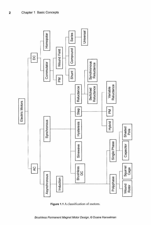
Figure 1.1 A classification of motors.

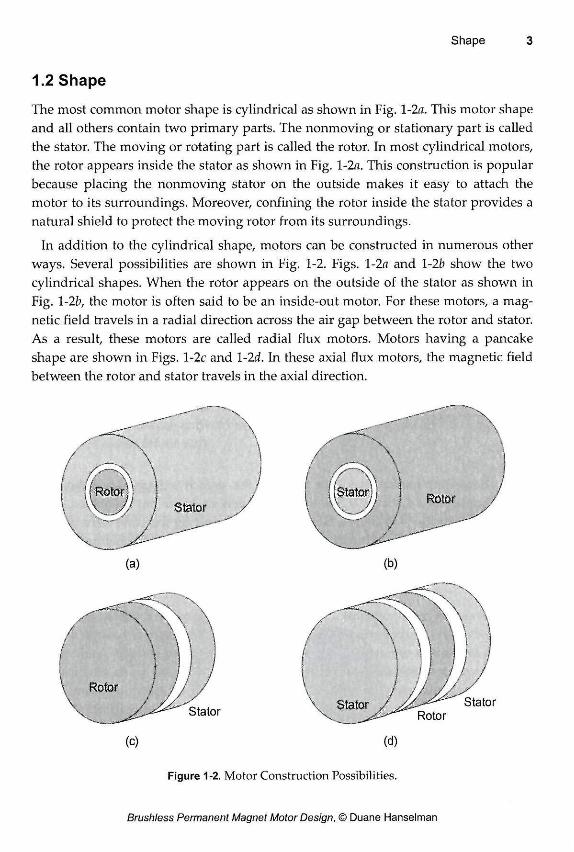
The most common motor shape is cylindrical as shown in Fig. 1-2a. This motor shape and all others contain two primary parts. The nonmoving or stationary part is called the stator. The moving or rotating part is called the rotor. In most cylindrical motors, the rotor appears inside the stator as shown in Fig. 1-2a. This construction is popular because placing the nonmoving stator on the outside makes it easy to attach the motor to its surroundings. Moreover, confining the rotor inside the stator provides a natural shield to protect the moving rotor from its surroundings.

In addition to the cylindrical shape, motors can be constructed in numerous other ways. Several possibilities are shown in Fig. 1-2. Figs. 1-2a and 1-2b show the two cylindrical shapes. When the rotor appears on the outside of the stator as shown in Fig. 1-2b, the motor is often said to be an inside-out motor. For these motors, a mag-netic field travels in a radial direction across the air gap between the rotor and stator. As a result, these motors are called radial flux motors. Motors having a pancake shape are shown in Figs. l-2c and 1-2d. In these axial flux motors, the magnetic field between the rotor and stator travels in the axial direction.

Figure 1-2. Motor Construction Possibilities.

Brushless PM motors can be built in all the shapes shown in Fig. 1-2 as well as in a number of other more creative shapes. All brushless PM motors are constructed with electrical windings on the stator and permanent magnets on the rotor. This construc-tion is one of the primary reasons for the increasing popularity of brushless PM motors. Because the windings remain stationary, no potentially troublesome moving electrical contacts, i.e., brushes are required. In addition, stationary windings are eas-ier to keep cool.

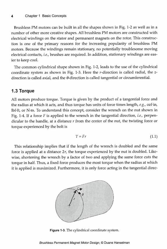
The common cylindrical shape shown in Fig. 1-2, leads to the use of the cylindrical coordinate system as shown in Fig. 1-3. Here the r-direction is called radial, the z-direction is called axial, and the ^-direction is called tangential or circumferential.

1.3 Torque

All motors produce torque. Torque is given by the product of a tangential force and the radius at which it acts, and thus torque has units of force times length, e.g., ozf in, lbf-ft, or N-m. To understand this concept, consider the wrench on the nut shown in Fig. 1-4. If a force F is applied to the wrench in the tangential direction, i.e., perpen-dicular to the handle, at a distance r from the center of the nut, the twisting force or torque experienced by the bolt is

This relationship implies that if the length of the wrench is doubled and the same force is applied at a distance 2r, the torque experienced by the nut is doubled. Like-wise, shortening the wrench by a factor of two and applying the same force cuts the torque in half. Thus, a fixed force produces the most torque when the radius at which it is applied is maximized. Furthermore, it is only force acting in the tangential direc-

T = Fr (1.1)

Figure 1-3. The cylindrical coordinate system.

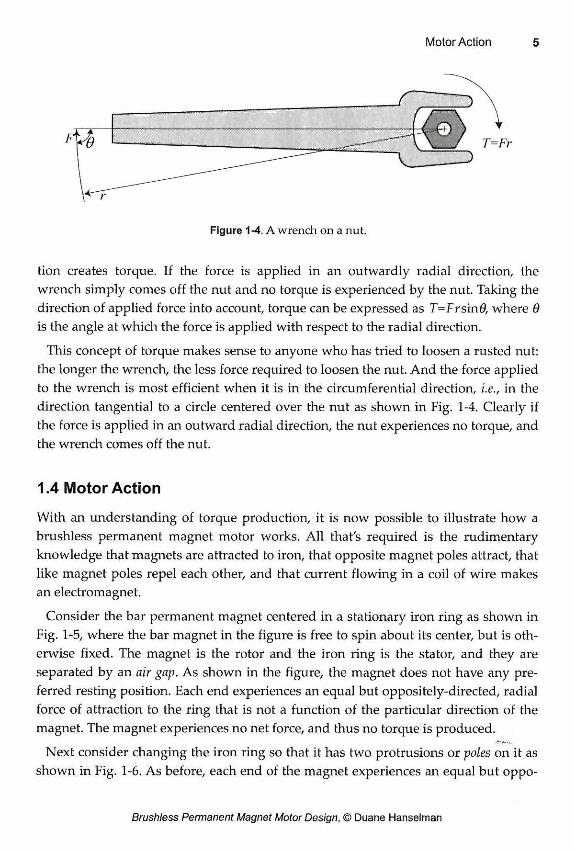
Figure 1-4. A wrench on a nut.

tion creates torque. If the force is applied in an outwardly radial direction, the wrench simply comes off the nut and no torque is experienced by the nut. Taking the direction of applied force into account, torque can be expressed as T=Frsin0, where 0 is the angle at which the force is applied with respect to the radial direction.

This concept of torque makes sense to anyone who has tried to loosen a rusted nut: the longer the wrench, the less force required to loosen the nut. And the force applied to the wrench is most efficient when it is in the circumferential direction, i.e., in the direction tangential to a circle centered over the nut as shown in Fig. 1-4. Clearly if the force is applied in an outward radial direction, the nut experiences no torque, and the wrench comes off the nut.

1.4 Motor Action

With an understanding of torque production, it is now possible to illustrate how a brushless permanent magnet motor works. All that's required is the rudimentary knowledge that magnets are attracted to iron, that opposite magnet poles attract, that like magnet poles repel each other, and that current flowing in a coil of wire makes an electromagnet.

Consider the bar permanent magnet centered in a stationary iron ring as shown in Fig. 1-5, where the bar magnet in the figure is free to spin about its center, but is oth-erwise fixed. The magnet is the rotor and the iron ring is the stator, and they are separated by an air gap. As shown in the figure, the magnet does not have any pre-ferred resting position. Each end experiences an equal but oppositely-directed, radial force of attraction to the ring that is not a function of the particular direction of the magnet. The magnet experiences no net force, and thus no torque is produced.

Next consider changing the iron ring so that it has two protrusions or poles on it as shown in Fig. 1-6. As before, each end of the magnet experiences an equal but oppo-

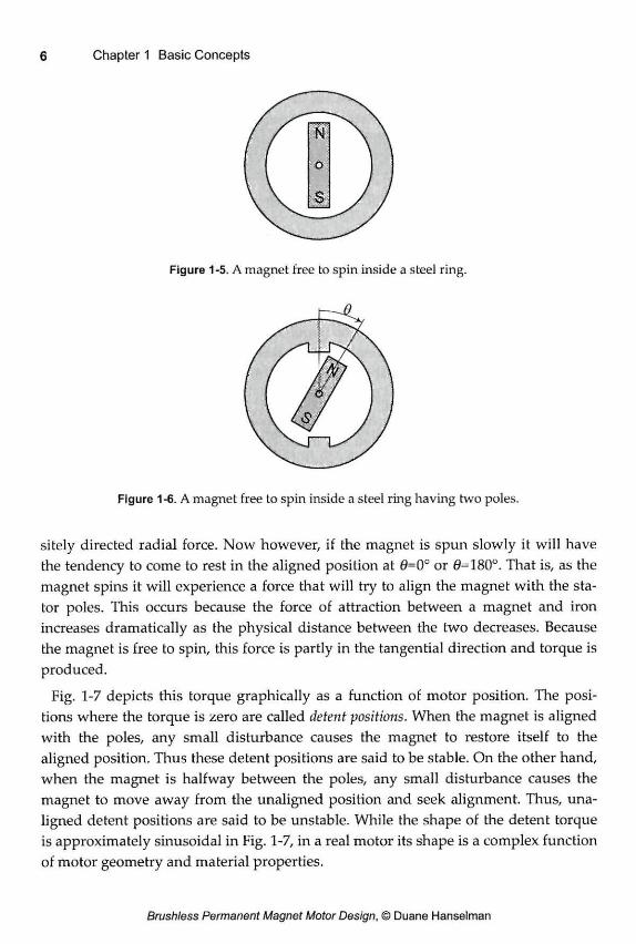
Figure 1-5. A magnet free to spin inside a steel ring.

sitely directed radial force. Now however, if the magnet is spun slowly it will have the tendency to come to rest in the aligned position at 0=0° or 0=180°. That is, as the magnet spins it will experience a force that will try to align the magnet with the sta-tor poles. This occurs because the force of attraction between a magnet and iron increases dramatically as the physical distance between the two decreases. Because the magnet is free to spin, this force is partly in the tangential direction and torque is produced.

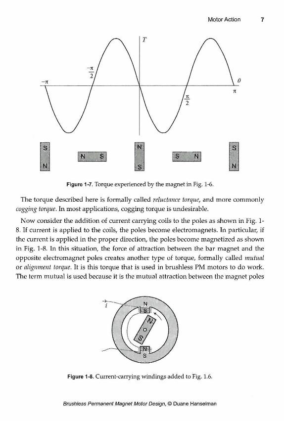
Fig. 1-7 depicts this torque graphically as a function of motor position. The posi-tions where the torque is zero are called detent positions. When the magnet is aligned with the poles, any small disturbance causes the magnet to restore itself to the aligned position. Thus these detent positions are said to be stable. On the other hand, when the magnet is halfway between the poles, any small disturbance causes the magnet to move away from the unaligned position and seek alignment. Thus, una-ligned detent positions are said to be unstable. While the shape of the detent torque is approximately sinusoidal in Fig. 1-7, in a real motor its shape is a complex function of motor geometry and material properties.

T

-7T

-7 i f \ ~2 \

\ 0

I— / 2 Tt

Figure 1-7. Torque experienced by the magnet in Fig. 1-6.

The torque described here is formally called reluctance torque, and more commonly cogging torque. In most applications, cogging torque is undesirable.

Now consider the addition of current carrying coils to the poles as shown in Fig. 1-8. If current is applied to the coils, the poles become electromagnets. In particular, if the current is applied in the proper direction, the poles become magnetized as shown in Fig. 1-8. In this situation, the force of attraction between the bar magnet and the opposite electromagnet poles creates another type of torque, formally called mutual or alignment torque. It is this torque that is used in brushless PM motors to do work. The term mutual is used because it is the mutual attraction between the magnet poles

Figure 1-8. Current-carrying windings added to Fig. 1.6.

that produces torque. The term alignment is used because the force of attraction seeks to align the bar magnet and coil-created magnet poles.

This torque could also be called repulsion torque, since if the current is applied in the opposite direction, the poles become magnetized in the opposite direction as shown in Fig. 1-9. In this situation the like poles repel, sending the bar magnet in the opposite direction. Since both of these scenarios involve the mutual interaction of the magnet poles, the torque mechanism is identical, and the term repulsion torque is not used.

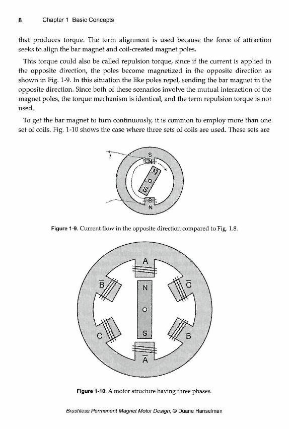
To get the bar magnet to turn continuously, it is common to employ more than one set of coils. Fig. 1-10 shows the case where three sets of coils are used. These sets are

Poles, Slots, Teeth, and Yokes 9

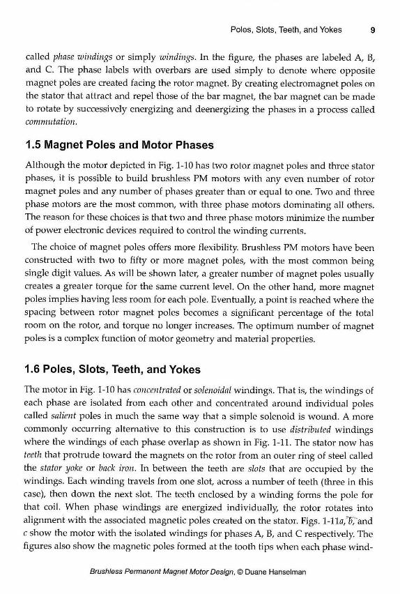
called phase windings or simply windings. In the figure, the phases are labeled A, B, and C. The phase labels with overbars are used simply to denote where opposite magnet poles are created facing the rotor magnet. By creating electromagnet poles on the stator that attract and repel those of the bar magnet, the bar magnet can be made to rotate by successively energizing and deenergizing the phases in a process called commutation.

1.5 Magnet Poles and Motor Phases

Although the motor depicted in Fig. 1-10 has two rotor magnet poles and three stator phases, it is possible to build brushless PM motors with any even number of rotor magnet poles and any number of phases greater than or equal to one. Two and three phase motors are the most common, with three phase motors dominating all others. The reason for these choices is that two and three phase motors minimize the number of power electronic devices required to control the winding currents.

The choice of magnet poles offers more flexibility. Brushless PM motors have been constructed with two to fifty or more magnet poles, with the most common being single digit values. As will be shown later, a greater number of magnet poles usually creates a greater torque for the same current level. On the other hand, more magnet poles implies having less room for each pole. Eventually, a point is reached where the spacing between rotor magnet poles becomes a significant percentage of the total room on the rotor, and torque no longer increases. The optimum number of magnet poles is a complex function of motor geometry and material properties.

1.6 Poles, Slots, Teeth, and Yokes

The motor in Fig. 1-10 has concentrated or solenoidal windings. That is, the windings of each phase are isolated from each other and concentrated around individual poles called salient poles in much the same way that a simple solenoid is wound. A more commonly occurring alternative to this construction is to use distributed windings where the windings of each phase overlap as shown in Fig. 1-11. The stator now has teeth that protrude toward the magnets on the rotor from an outer ring of steel called the stator yoke or back iron. In between the teeth are slots that are occupied by the windings. Each winding travels from one slot, across a number of teeth (three in this case), then down the next slot. The teeth enclosed by a winding forms the pole for that coil. When phase windings are energized individually, the rotor rotates into alignment with the associated magnetic poles created on the stator. Figs. l-lla,"B',and c show the motor with the isolated windings for phases A, B, and C respectively. The figures also show the magnetic poles formed at the tooth tips when each phase wind-

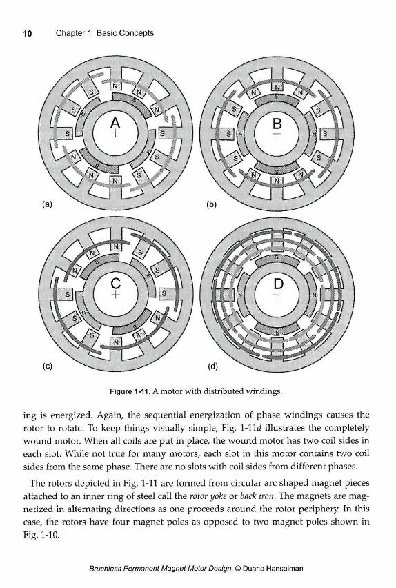
Figure 1-11. A motor with distributed windings.

ing is energized. Again, the sequential energization of phase windings causes the rotor to rotate. To keep things visually simple, Fig. 1-11 d illustrates the completely wound motor. When all coils are put in place, the wound motor has two coil sides in each slot. While not true for many motors, each slot in this motor contains two coil sides from the same phase. There are no slots with coil sides from different phases.

The rotors depicted in Fig. 1-11 are formed from circular arc shaped magnet pieces attached to an inner ring of steel call the rotor yoke or back iron. The magnets are mag-netized in alternating directions as one proceeds around the rotor periphery. In this case, the rotors have four magnet poles as opposed to two magnet poles shown in Fig. 1-10.

Mechanical and Electrical Measures 11

The motor cross sections shown in Fig. 1-11 are more representative of actual motors than those shown earlier, but they are still much simpler than real motors. In later chapters, a variety of more practical motor construction details will be pre-sented.

1.7 Mechanical and Electrical Measures

In electric motors it is common to define two related measures of position and speed. Mechanical position and speed are the respective position and speed of the rotor shaft. When the rotor shaft makes one complete revolution, it traverses 360 mechani-cal degrees (°M) or 2n mechanical radians (radM). Having made this revolution, the rotor is right back where it started.

Electrical position is defined such that movement of the rotor by 360 electrical degrees (°E) or 2n electrical radians (radE) puts the rotor back in an identical mag-netic orientation. In Fig. 1-10, mechanical and electrical position are identical since the rotor must rotate 360°M to reach the same magnetic orientation. On the other hand, in Fig. 1-11 the rotor need only move 180 °M to have the same magnetic orien-tation. Thus, 360°E is the same as 180°M for this case. Based on these two cases, it is easy to see that the relationship between electrical and mechanical position is related to the number of magnet poles on the rotor. If Nm is the number of magnet poles on the rotor facing the air gap, i.e., Nm= 2 for Fig. 1-10 and Nm= 4 for Fig. 1-11, this rela-tionship can be stated as

where 6e and 0 m are electrical and mechanical position respectively. Since magnets always have two poles, it is common to define a pole pair as one North and one South magnet pole facing the air gap. In this case, the number of pole pairs is equal to Np= NJ2 and the above relationship is simply

0e = N r 9 m (1.3)

Differentiating (1.3) with respect to time gives the relationship between electrical and mechanical frequency or speed as

= Np(Om (1.4)

where coc and com are electrical and mechanical frequencies respectively in radians per second. This relationship can also be stated in terms of Hertz (cycles per second) as

fc=Hpfln (1.5)

where/„,= (0m/(2ri). Later when harmonics of fe are discussed, fc will be called the fun-damental electrical frequency.

It is common practice to specify motor mechanical speed, S, in revolutions per min-ute (rpm). For reference, the relationships among S,f„„ and fe are given by

* c S

^ = 3 0 S - l o M

N Nv fe = — = — S (1.7) J e 120 60 V ;

This last equation is useful because it describes the rate or frequency at which com-mutation must occur for the motor to turn at a given speed in rpm. The inverse of this frequency gives the commutation time period, i.e., the length of time over which the energizing of a phase completes one cycle of operation.

The fundamental electrical frequency/,, influences the design of the power electron-ics used to drive the motor. As fe increases, the power electronics must act faster to keep the motor shaft turning. This implies that the power electronics become more expensive as fe increases. Because of this, it is common to use fewer magnet poles, i.e., reduce N,„, for motors designed to operate at high speeds. However, reducing N„, does not come without a penalty. As the magnet pole count decreases, the torque production efficiency drops. Therefore, one must find a compromise between power electronics cost and torque production efficiency when choosing the number of mag-net poles.

Variables such as 9 and co are used in this text both with and without various sub-scripts to denote positions and velocities. In some situations, these variables describe quantities in electrical measure; in other places they describe quantities in mechanical measure. In all cases, the subscript e denotes electrical measure; whereas the sub-script m denotes mechanical measure. When these subscripts are not used, the con-text of passage where they appear clarifies their unit measure.

A fundamental question in motor design is: How big does a motor have to be to pro-duce a required torque? For radial flux motors the answer to this question is often stated as

T = kD2L (1.8)

where T is torque, k is a constant, D is the rotor diameter, and L is the axial rotor length. To understand this relationship, reconsider the motor shown in Fig. 1-10.

First assume that the motor has an axial length (depth into page) equal to L. For this length, a certain torque TL is available. Now if this motor is duplicated, added to the end of the original motor, and the rotor shafts connected together, the total torque available becomes the sum of that from each motor, namely T = T[+ T . That is, an effective doubling of the axial rotor length to 2L doubles the available torque. Thus, torque is linearly proportional to L as shown in (1.8).

Understanding the D2 relationship requires a little more effort. In the discussion of the wrench and nut shown in Fig. 1-4, it was stated that a given force produces a torque that is proportional to radius, i.e., D/2. Therefore, torque is at least linearly proportional to diameter. However, it can be argued that the ability to produce force is also linearly proportional to diameter. This follows because the rotor perimeter increases linearly with diameter, e.g., the circumference of a circle is equal to nD. A simple way to see this relationship is to compare the simple motor in Fig. 1-10 to that in Fig. 1-11. If the motor in Fig. 1-10 produces a torque T, then the motor in Fig. 1-11 should produce a torque equal to 2T because twice the magnets are producing twice the force. Clearly as diameter increases, there is more and more room for magnets around the rotor. So it makes sense that the ability to produce force increases linearly with diameter. Combining these two contributing factors leads to the desired rela-tionship (1.8) that torque is proportional to diameter squared.

1.9 Units

Unless specifically noted otherwise, this text utilizes the International System of Units (SI units). Doing so eliminates the need for conversion factors that often complicate expressions and derivations. On the other hand, SI units are not universally used in practice. Several other systems of units are commonly used; each with its own.advan-tages and disadvantages. It is assumed that the reader can convert the expressions and quantities in this text to the system of units of their choice.

14 Chapter 1 Basic Concepts

1.10 Summary

This chapter developed the basic concepts involved in brushless PM motor design. Both radial flux and axial flux shapes were described. The relationship between torque and force was developed and basic properties of magnets were used to intui-tively describe how a motor works. Along the way, the ideas of coils, windings,

2 phases, poles, slots, teeth, and yokes were introduced. The commonly held D L siz-ing relationship was also justified intuitively. The purpose of the remaining chapters is to use and expand the intuition gained in this chapter to develop quantitative expressions describing motor operation and performance.

Brushless permanent magnet motor operation relies on the conversion of energy from electrical to magnetic to mechanical. Because magnetic energy plays a central role in the production of torque, it is necessary to formulate methods for computing it. Magnetic energy is highly dependent upon the spatial distribution of a magnetic field, i.e., how it is distributed within an apparatus. For brushless permanent magnet motors, this means finding the magnetic field distribution within the motor.

There are numerous ways to determine the magnetic field distribution within an apparatus. For very simple geometries, the magnetic field distribution can be found analytically. However, in most cases, the field distribution can only be approximated. Magnetic field approximations appear in two general forms. In the first, the direction of the magnetic field is assumed to be known everywhere within the apparatus. This leads to magnetic circuit analysis, which is analogous to electric circuit analysis. In the other form, the apparatus is discretized geometrically, and the magnetic field is numerically computed at discrete points in the apparatus. From this information, the magnitude and direction of the magnetic field can be approximated throughout the apparatus. This approach is commonly called finite element analysis, and it embodies a variety of similar mathematical methods known as the finite difference method, the finite element method, and the boundary element method.

Of these two magnetic field approximations, finite element analysis produces the most accurate results if the geometric discretization is fine enough. While the power of computers now allows one to generate finite element analysis solutions in reason-able time, finite element analysis requires a detailed model of the apparatus that may take many hours to produce. In addition to the time involved, finite element analysis produces a purely numerical solution. The solution is typically composed of the potential at thousands of points within the apparatus. The relationship between geo-metrical parameters and the resulting change in the magnetic field distribution are not related analytically. Thus many finite element solutions are usually required to develop basic insight into the effect of various parameters on the magnetic field dis-tribution. Because of these disadvantages, finite element analysis is not used exten-

sively as a design tool. Rather, it is most often used to confirm or improve the results of analytical design work. For this task, finite element analysis is indispensable.

As opposed to the complexity and numerical nature of finite element analysis, the simplicity and analytic properties of magnetic circuit analysis make it the most com-monly used magnetic field approximation method for much design work. By making the assumption that the direction of the magnetic field is known throughout an appa-ratus, magnetic circuit analysis allows one to approximate the field distribution ana-lytically. Because of this analytical relationship, the geometry of a problem is clearly related to its field distribution, thereby providing substantial design insight. A major weakness of the magnetic circuit approach is that it is often difficult to determine the magnetic field direction throughout an apparatus. Moreover, predetermining the magnetic field direction requires subjective foresight that is influenced by the experi-ence of the person using magnetic circuit analysis. Despite these weaknesses, mag-netic circuit analysis is very useful for designing brushless permanent magnet motors. For this reason, magnetic circuit analysis concepts are developed in this chapter.

2.1 Magnetic Circuit Concepts

Basic Relationships Two vector quantities, B and H, describe a magnetic field. The flux density B can be thought of as the density of magnetic field flowing through a given area of material, and the field intensity H is the resulting change in the intensity of the magnetic field due to the interaction of B with the material it encounters. For magnetic materials common to motor design, B and H are collinear. That is, they are oriented in the same coordinate direction within a given material. Fig. 2-1 illustrates these relationships for a differential size block of material. In this figure, B is directed perpendicularly through the block in the z-direction, and H is the change in the field intensity in the z-direction. In general, the relationship between B and H is a nonlinear, multivalued function of the material. However, for many materials this relationship is linear or nearly linear over a sufficiently large operating range. In this case, B and H are line-arly related and written as

B = nH (2.1)

where n is the permeability of the material.

Magnetic circuit analysis is based on the assumptions of material linearity and the colinearity of B and H. Two fundamental equations lead to magnetic circuit analysis.

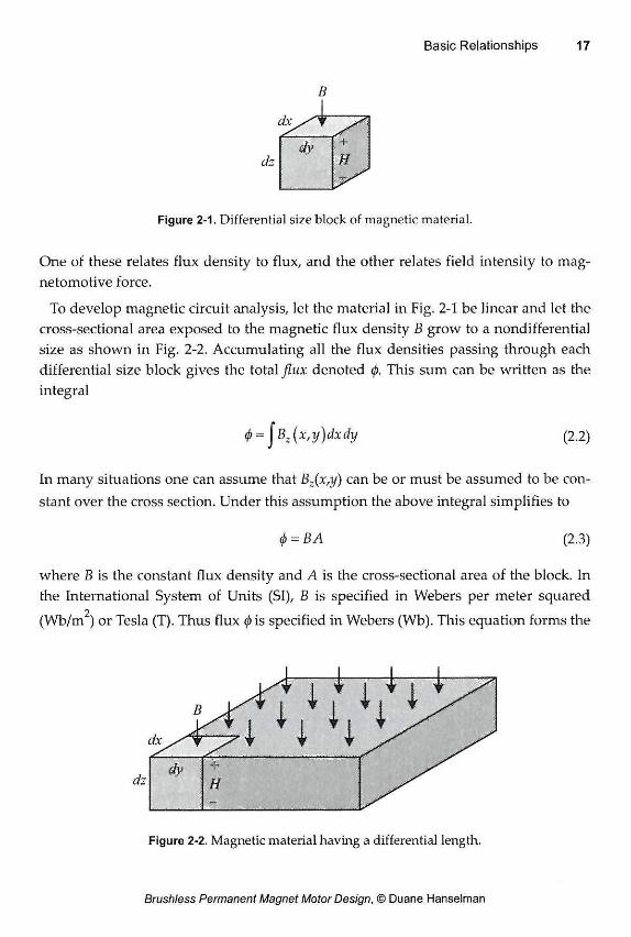
Figure 2-1. Differential size block of magnetic material.

One of these relates flux density to flux, and the other relates field intensity to mag-netomotive force.

To develop magnetic circuit analysis, let the material in Fig. 2-1 be linear and let the cross-sectional area exposed to the magnetic flux density B grow to a nondifferential size as shown in Fig. 2-2. Accumulating all the flux densities passing through each differential size block gives the total flux denoted (p. This sum can be written as the integral

(f> = \Bz(x,y)dxdy (2.2)

In many situations one can assume that Bz(x,y) can be or must be assumed to be con-stant over the cross section. Under this assumption the above integral simplifies to

(p = BA (2.3)

where B is the constant flux density and A is the cross-sectional area of the block. In the International System of Units (SI), B is specified in Webers per meter squared (Wb/m ) or Tesla (T). Thus flux 0 is specified in Webers (Wb). This equation forms the

Figure 2-2. Magnetic material having a differential length.

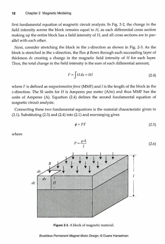
first fundamental equation of magnetic circuit analysis. In Fig. 2-2, the change in the field intensity across the block remains equal to H, as each differential cross section making up the entire block has a field intensity of H, and all cross sections are in par-allel with each other.

Next, consider stretching the block in the z-direction as shown in Fig. 2-3. As the block is stretched in the z-direction, the flux 0 flows through each succeeding layer of thickness dz creating a change in the magnetic field intensity of H for each layer. Thus, the total change in the field intensity is the sum of each differential amount,

where F is defined as magnetomotive force (MMF) and / is the length of the block in the z-direction. The SI units for H is Amperes per meter (A/m) and thus MMF has the units of Amperes (A). Equation (2.4) defines the second fundamental equation of magnetic circuit analysis.

Connecting these two fundamental equations is the material characteristic given in (2.1). Substituting (2.3) and (2.4) into (2.1) and rearranging gives

(2.4)

4> = PF (2.5)

where

(2.6)

dz

I

Figure 2-3. A block of magnetic material.

is defined as the permeance of the material having a cross-sectional area A, length I, and permeability \i. Permeance is described in units of Webers per Ampere (Wb/A) or Henries (H). Materials having higher permeability have greater permeance, which promotes greater flux flow through them.

Equation (2.5) is analogous to Ohm's law, I=GV. Flux flows in closed paths just as current does; F is magnetomotive force (MMF) just as voltage is electromotive force (EMF), and the conductance of a rectangular block of resistive material is identical to the permeance equation (2.6) with conductivity replacing permeability.

The inverse of permeance is reluctance and is given by

In terms of reluctance, (2.5) can be rewritten as

which is analogous to Ohm's law written as V=IR, with reluctance being analogous to resistance. At this point the analogy between electric and magnetic circuits ends because current flow through a resistance constitutes energy dissipation, whereas flux flow through a reluctance constitutes energy storage.

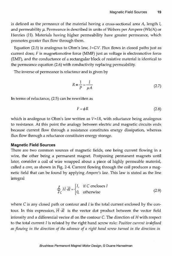
Magnetic Field Sources There are two common sources of magnetic fields, one being current flowing in a wire, the other being a permanent magnet. Postponing permanent magnets until later, consider a coil of wire wrapped about a piece of highly permeable material, called a core, as shown in Fig. 2-4. Current flowing through the coil produces a mag-netic field that can be found by applying Ampere's law. This law is stated as the line integral

where C is any closed path or contour and / is the total current enclosed by the con-tour. In this expression, H • dl is the vector dot product between the vector field intensity and a differential vector dl on the contour C. The direction of H with respect to the total current I is related by the right hand screw rule: Positive current is-defined as flowing in the direction of the advance of a right hand screw turned in the direction in

F = <f>R (2.8)

I, if C encloses I 0, otherwise (2.9)

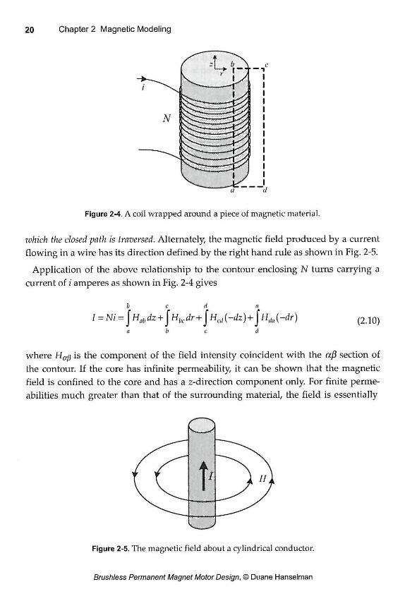
Figure 2-4. A coil wrapped around a piece of magnetic material.

which the closed path is traversed. Alternately, the magnetic field produced by a current flowing in a wire has its direction defined by the right hand rule as shown in Fig. 2-5.

Application of the above relationship to the contour enclosing N turns carrying a current of i amperes as shown in Fig. 2-4 gives

b e d a I = Ni = j Hab dz + jHbcdr+j Hcd (-dz)+J* Hda (-dr) ( 2 .10)

a b c d

where Haß is the component of the field intensity coincident with the aß section of the contour. If the core has infinite permeability, it can be shown that the magnetic field is confined to the core and has a z-direction component only. For finite perme-abilities much greater than that of the surrounding material, the field is essentially

confined to the core also; thus all terms in the above equation except the first, are zero. Using this assumption, the above simplifies to

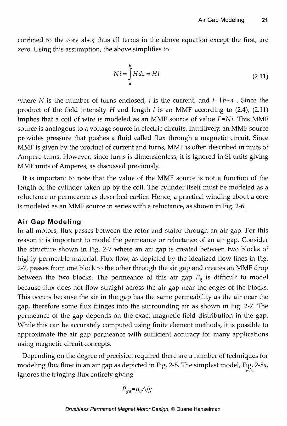
where N is the number of turns enclosed, i is the current, and l=\b-a\. Since the product of the field intensity H and length I is an MMF according to (2.4), (2.11) implies that a coil of wire is modeled as an MMF source of value F=Ni. This MMF source is analogous to a voltage source in electric circuits. Intuitively, an MMF source provides pressure that pushes a fluid called flux through a magnetic circuit. Since MMF is given by the product of current and turns, MMF is often described in units of Ampere-turns. However, since turns is dimensionless, it is ignored in SI units giving MMF units of Amperes, as discussed previously.

It is important to note that the value of the MMF source is not a function of the length of the cylinder taken up by the coil. The cylinder itself must be modeled as a reluctance or permeance as described earlier. Hence, a practical winding about a core is modeled as an MMF source in series with a reluctance, as shown in Fig. 2-6.

Air Gap Mode l ing In all motors, flux passes between the rotor and stator through an air gap. For this reason it is important to model the permeance or reluctance of an air gap. Consider the structure shown in Fig. 2-7 where an air gap is created between two blocks of highly permeable material. Flux flow, as depicted by the idealized flow lines in Fig. 2-7, passes from one block to the other through the air gap and creates an MMF drop between the two blocks. The permeance of this air gap Pg is difficult to model because flux does not flow straight across the air gap near the edges of the blocks. This occurs because the air in the gap has the same permeability as the air near the gap, therefore some flux fringes into the surrounding air as shown in Fig. 2-7. The permeance of the gap depends on the exact magnetic field distribution in the gap. While this can be accurately computed using finite element methods, it is possible to approximate the air gap permeance with sufficient accuracy for many applications using magnetic circuit concepts.

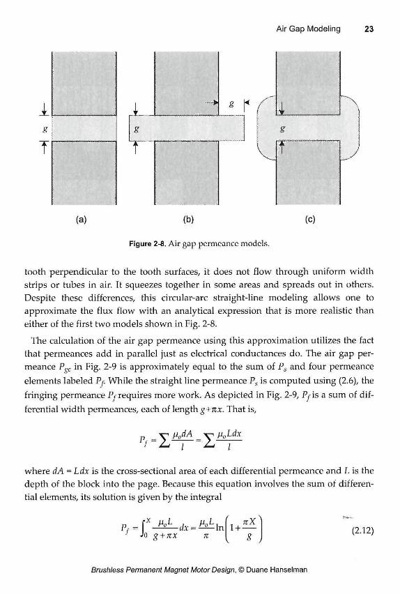
Depending on the degree of precision required there are a number of techniques for modeling flux flow in an air gap as depicted in Fig. 2-8. The simplest model, Fig. 2-8a, ignores the fringing flux entirely giving

b (2.11)

a

Pga=^8

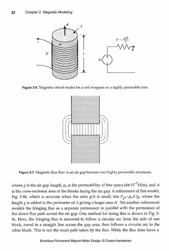
Figure 2-7. Magnetic flux flow in an air gap between two highly permeable structures.

_7

where g is the air gap length, fi0 is the permeability of free space (471-10 H/m), and A is the cross-sectional area of the blocks facing the air gap. A refinement of this model, Fig. 2-8b, which is accurate when the ratio g/A is small, lets Pgh=n0A'/g, where the length g is added to the perimeter of A giving a larger area A'. Yet another refinement models the fringing flux as a separate permeance in parallel with the permeance of the direct flux path across the air gap. One method for doing this is shown in Fig. 2-8c. Here, the fringing flux is assumed to follow a circular arc from the side of one block, travel in a straight line across the gap area, then follows a circular arc to the other block. This is not the exact path taken by the flux. While the flux does leave a

(a) (b) (c)

Figure 2-8. Air gap permeance models.

tooth perpendicular to the tooth surfaces, it does not flow through uniform width strips or tubes in air. It squeezes together in some areas and spreads out in others. Despite these differences, this circular-arc straight-line modeling allows one to approximate the flux flow with an analytical expression that is more realistic than either of the first two models shown in Fig. 2-8.

The calculation of the air gap permeance using this approximation utilizes the fact that permeances add in parallel just as electrical conductances do. The air gap per-meance PgC in Fig. 2-9 is approximately equal to the sum of Ps and four permeance elements labeled Pf. While the straight line permeance Ps is computed using (2.6), the fringing permeance Pf requires more work. As depicted in Fig. 2-9, Py is a sum of dif-ferential width permeances, each of length g+iix. That is,

¡d0dA Y 1 A'o Ldx I

where dA = Ldx is the cross-sectional area of each differential permeance and L is the depth of the block into the page. Because this equation involves the sum of differen-tial elements, its solution is given by the integral

p/ = 'L 0 g + 7tX 71 1 +

7tX (2.12)

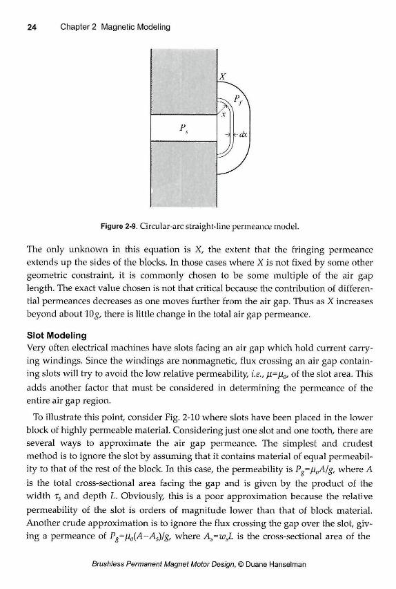
Figure 2-9. Circular-arc straight-line permeance model.

The only unknown in this equation is X, the extent that the fringing permeance extends up the sides of the blocks. In those cases where X is not fixed by some other geometric constraint, it is commonly chosen to be some multiple of the air gap length. The exact value chosen is not that critical because the contribution of differen-tial permeances decreases as one moves further from the air gap. Thus as X increases beyond about lOg, there is little change in the total air gap permeance.

Slot Modeling Very often electrical machines have slots facing an air gap which hold current carry-ing windings. Since the windings are nonmagnetic, flux crossing an air gap contain-ing slots will try to avoid the low relative permeability, i.e., /i=pi0, of the slot area. This adds another factor that must be considered in determining the permeance of the entire air gap region.

To illustrate this point, consider Fig. 2-10 where slots have been placed in the lower block of highly permeable material. Considering just one slot and one tooth, there are several ways to approximate the air gap permeance. The simplest and crudest method is to ignore the slot by assuming that it contains material of equal permeabil-ity to that of the rest of the block. In this case, the permeability is P?=/i0A/g, where A is the total cross-sectional area facing the gap and is given by the product of the width TS and depth L. Obviously, this is a poor approximation because the relative permeability of the slot is orders of magnitude lower than that of block material. Another crude approximation is to ignore the flux crossing the gap over the slot, giv-ing a permeance of Pg=/J0(A-As)/g, where As=wsL is the cross-sectional area of the

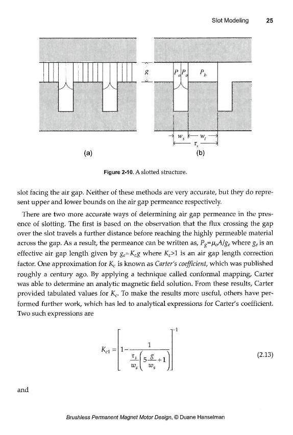
(a)

P. P P,

w,

(b)

Figure 2-10. A slotted structure.

slot facing the air gap. Neither of these methods are very accurate, but they do repre-sent upper and lower bounds on the air gap permeance respectively.

There are two more accurate ways of determining air gap permeance in the pres-ence of slotting. The first is based on the observation that the flux crossing the gap over the slot travels a further distance before reaching the highly permeable material across the gap. As a result, the permeance can be written as, Pg=fi0A/ge where ge is an effective air gap length given by ge=Kcg where Kc> 1 is an air gap length correction factor. One approximation for Kc is known as Carter's coefficient, which was published roughly a century ago. By applying a technique called conformal mapping, Carter was able to determine an analytic magnetic field solution. From these results, Carter provided tabulated values for Kc. To make the results more useful, others have per-formed further work, which has led to analytical expressions for Carter's coefficient. Two such expressions are

(2.13)

and

1 / \

5 — + 1 Ws ws s

KC2 = 2 wa

7TTc tan -l

2g - — I n

UK 4 we

-l

(2.14)

The other method for determining the air gap permeance utilizes the circular arc, straight line modeling discussed earlier. This method is demonstrated in Fig. 2-10fr. Following an approach similar to that described by (2.12), the permeance of the air gap over one slot pitch Ts can be written as

P=2Pa+Pb=/u0L w +—In g 7t

1 + 7tWs

where L is the depth of the block into the page. With some algebraic manipulation, this solution can also be written in the form of an air gap length correction factor as described in the preceding paragraph. In this case, Kc is given by

*c3 = 1 - ^ + iS - ln rc ktc

1 + KWC

4g

-l (2.15)

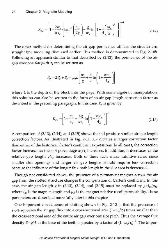
A comparison of (2.13), (2.14), and (2.15) shows that all produce similar air gap length correction factors. As illustrated in Fig. 2-11, dictates a larger correction factor than either of the historical Carter's coefficient expressions. In all cases, the correction factor increases as the slot percentage ivs/zs increases. In addition, it decreases as the relative gap length g/rs increases. Both of these facts make intuitive sense since smaller slot openings and larger air gap lengths should require less correction because the influence of the longer flux path length in the slot area is decreased.

Though not considered above, the presence of a permanent magnet across the air gap from the slotted structure changes the computation of Carter's coefficient. In this case, the air gap length g in (2.13), (2.14), and (2.15) must be replaced by g+lm/^R, where l m is the magnet length and [Ir is the magnet relative recoil permeability. These parameters are described more fully later in this chapter.

One important consequence of slotting shown in Fig. 2-12 is that the presence of slots squeezes the air gap flux into a cross-sectional area (1-wJt s) times smaller than the cross-sectional area of the entire air gap over one slot pitch. Thus the average flux density B=<p/A at the base of the teeth is greater by a factor of (1 -wjrs) \ The impor-

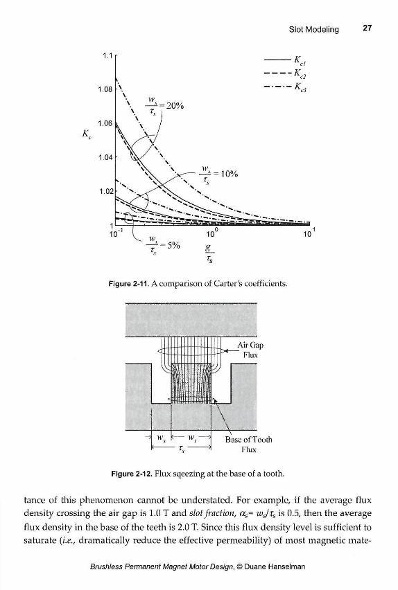
Figure 2-11. A comparison of Carter's coefficients.

Figure 2-12. Flux sqeezing at the base of a tooth.

tance of this phenomenon cannot be understated. For example, if the average flux density crossing the air gap is 1.0 T and slot fraction, 0^= ws/ts is 0.5, then the average flux density in the base of the teeth is 2.0 T. Since this flux density level is sufficient to saturate (i.e., dramatically reduce the effective permeability) of most magnetic mate-

rials, there is an upper limit to the achievable air gap flux density in a motor. Later this will be shown to be a crucial factor in motor performance.

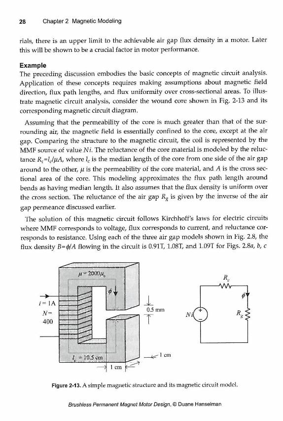
Example The preceding discussion embodies the basic concepts of magnetic circuit analysis. Application of these concepts requires making assumptions about magnetic field direction, flux path lengths, and flux uniformity over cross-sectional areas. To illus-trate magnetic circuit analysis, consider the wound core shown in Fig. 2-13 and its corresponding magnetic circuit diagram.

Assuming that the permeability of the core is much greater than that of the sur-rounding air, the magnetic field is essentially confined to the core, except at the air gap. Comparing the structure to the magnetic circuit, the coil is represented by the MMF source of value Ni. The reluctance of the core material is modeled by the reluc-tance Rc=lcll±A, where lc is the median length of the core from one side of the air gap around to the other, ji is the permeability of the core material, and A is the cross sec-tional area of the core. This modeling approximates the flux path length around bends as having median length. It also assumes that the flux density is uniform over the cross section. The reluctance of the air gap Rg is given by the inverse of the air gap permeance discussed earlier.

The solution of this magnetic circuit follows Kirchhoff's laws for electric circuits where MMF corresponds to voltage, flux corresponds to current, and reluctance cor-responds to resistance. Using each of the three air gap models shown in Fig. 2.8, the flux density B=(p/A flowing in the circuit is 0.91T, 1.08T, and 1.09T for Figs. 2.8a, b, c

0.5 mm

Rc

-M/V

<b 1 cm

Figure 2-13. A simple magnetic structure and its magnetic circuit model.

respectively, where X=10g is used for Fig. 2-8c in (2.12). Solving for the MMF across the air gap Fg=(j)Rs for each case and expressing the results in terms of percentages with respect to the MMF source of Ni=400 gives 90.5%, 88.7%, and 88.6% for the three respective cases. These results show that the two air gap models that include a cor-rection for fringing lead to nearly identical results, with these results differing signifi-cantly from the case in Fig. 2-8a where fringing is ignored. In addition, for all three cases, the air gap dominates the circuit because approximately 90% of the available magnetomotive force is required to push the flux across the air gap.

The fact that the air gap dominates the magnetic circuit has profound implications in practice. For analytic work, it allows one to neglect the reluctance of the core in many cases, thereby simplifying the analysis considerably. The dominance of the air gap also implies that the exact magnetic characteristics of the core do not have a great effect on the solution provided that the permeability of the core remains high. This is fortunate because the core is commonly made from materials having nonlinear mag-netic properties.

Before moving on it is important to note that the magnetic circuit shown in Fig. 2-13 ignores flux in the air surrounding the core away from the air gap. In electric circuits the difference in conductivity between conductors (e.g., wires) and insulators (e.g., air) is on the order of 10 . As a result, current stays confined to the conductors in an electric circuit. On the other hand, in a magnetic circuit the difference in permeability between conductors (e.g., cores) and insulators (e.g., air) is only typically on the order

2 3 of 10 to 10 . Therefore, some magnetic flux strays out of core material into the sur-rounding air. Inclusion of this stray flux requires identifying the flux paths involved, determining a reluctance or permeance model for them, then solving the resulting magnetic circuit. Clearly this complicates magnetic circuit analysis immensely. For this reason, only dominant fringing flux is taken into account, such as that surround-ing a primary air gap as shown in Figs. 2-8b and 2-8c.

Magnetic circuit analysis does not lead to exact magnetic field solutions. However, it often leads to analytic solutions that are conducive to the formulation of design equations. Finite element analysis leads to much more accurate magnetic field solu-tions because it models all flux fringing paths, but it only provides a numerical solu-tion. In a sense, magnetic circuit analysis solves problems from a macroperspective, whereas finite element analysis solves problems from a microperspective. These two approaches complement each other. The strengths of one approach are the weak-nesses of the other. Both are valuable in the design of brushless permanent magnet motors.

2.2 Magnetic Materials

Permeability

As stated in (2.1), in linear materials B and H are related by, B=/iH, where /i is the permeability of the material. For convenience, it is common to express permeability with respect to the permeability of free space, o=4TI*10 H/m. In doing so, a dimensionless relative permeability is defined as

(2-16) r-o

and (2.1) is rewritten as B=fj.r[i0H. As a result of this relationship, materials having jXr~ 1 are commonly called nonmagnetic materials, while those with much greater permeability are called magnetic materials. Permeability as defined by (2.1) and (2.16) applies strictly to materials that are linear, homogeneous (i.e., have uniform properties), and isotropic (i.e., have the same properties in all directions). Despite this fact, however, (2.1) and (2.16) are used extensively because they approximate the actual properties of more complex magnetic materials with sufficient accuracy over a sufficiently wide operating range.

Ferromagnetic materials, especially electrical steels, are the most common magnetic materials used in motor construction. The permeability of these materials is nonlin-ear and multivalued, making exact analysis extremely difficult. In addition to the permeability being a nonlinear, saturating function of the field intensity, the multival-ued nature of the permeability means that the flux density through the material is not unique for a given field intensity, but rather is a function of the past history of the field intensity. Because of this behavior, the magnetic properties of a ferromagnetic material are often described graphically in terms of its B-H curve, hysteresis loop, and core losses.

Ferromagnetic Materials Figure 2-14 shows the B-H curve and several hysteresis loops for a typical ferromag-netic material. Hysteresis loops are formed by applying sinusoidal excitation of dif-ferent amplitudes to the material and plotting B versus H. The B-H curve is formed by connecting the tips or extremes of the hysteresis loops together to form a smooth curve. The B-H curve, or DC magnetization curve, represents an average material characteristic that reflects the nonlinear property of the permeability, but ignores its multivalued property.

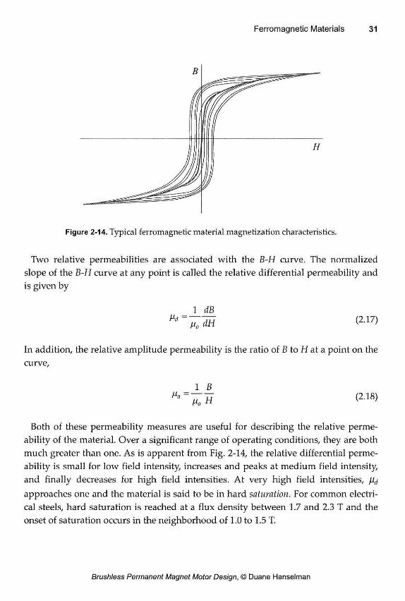
Figure 2-14. Typical ferromagnetic material magnetization characteristics.

Two relative permeabilities are associated with the B-H curve. The normalized slope of the B-H curve at any point is called the relative differential permeability and is given by

Pd = 1 dB

Po dti (2.17)

In addition, the relative amplitude permeability is the ratio of B to H at a point on the

curve,

Pa -—77 Po H (2.18)

Both of these permeability measures are useful for describing the relative perme-ability of the material. Over a significant range of operating conditions, they are both much greater than one. As is apparent from Fig. 2-14, the relative differential perme-ability is small for low field intensity, increases and peaks at medium field intensity, and finally decreases for high field intensities. At very high field intensities, fa approaches one and the material is said to be in hard saturation. For common electri-cal steels, hard saturation is reached at a flux density between 1.7 and 2.3 T and the onset of saturation occurs in the neighborhood of 1.0 to 1.5 T.

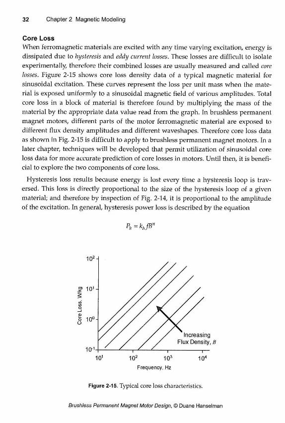
Core Loss When ferromagnetic materials are excited with any time varying excitation, energy is dissipated due to hysteresis and eddy current losses. These losses are difficult to isolate experimentally, therefore their combined losses are usually measured and called core losses. Figure 2-15 shows core loss density data of a typical magnetic material for sinusoidal excitation. These curves represent the loss per unit mass when the mate-rial is exposed uniformly to a sinusoidal magnetic field of various amplitudes. Total core loss in a block of material is therefore found by multiplying the mass of the material by the appropriate data value read from the graph. In brushless permanent magnet motors, different parts of the motor ferromagnetic material are exposed to different flux density amplitudes and different waveshapes. Therefore core loss data as shown in Fig. 2-15 is difficult to apply to brushless permanent magnet motors. In a later chapter, techniques will be developed that permit utilization of sinusoidal core loss data for more accurate prediction of core losses in motors. Until then, it is benefi-cial to explore the two components of core loss.

Hysteresis loss results because energy is lost every time a hysteresis loop is trav-ersed. This loss is directly proportional to the size of the hysteresis loop of a given material; and therefore by inspection of Fig. 2-14, it is proportional to the amplitude of the excitation. In general, hysteresis power loss is described by the equation

Pu=k„fB"

Frequency, Hz

where k/, is a constant that depends on the material type and dimensions, / is the fre-quency of applied excitation, B is the flux density amplitude within the material, and n is a material dependent exponent usually between 1.5 and 2.5.

Eddy current loss is caused by electric currents induced within the ferromagnetic material under time varying excitation. These induced eddy currents circulate within the material dissipating power (i.e., I R losses) due to the resistivity of the material. Eddy current power loss is approximately described by the relationship

Pe = keh2 f2B2

where h is the material thickness and ke is a material dependent constant. In this case, power lost is proportional to the square of frequency, flux density amplitude, and material thickness in the plane perpendicular to the magnetic field flow. Therefore, one would expect hysteresis loss to dominate at low frequencies and eddy current loss to dominate at higher frequencies.

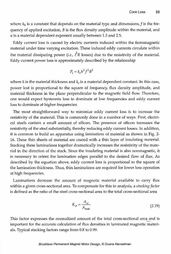
The most straightforward way to minimize eddy current loss is to increase the resistivity of the material. This is commonly done in a number of ways. First, electri-cal steels contain a small amount of silicon. The presence of silicon increases the resistivity of the steel substantially, thereby reducing eddy current losses. In addition, it is common to build an apparatus using laminations of material as shown in Fig. 2-16. These thin sheets of material are coated with a thin layer of insulating material. Stacking these laminations together dramatically increases the resistivity of the mate-rial in the direction of the stack. Since the insulating material is also nonmagnetic, it is necessary to orient the lamination edges parallel to the desired flow of flux. As described by the equation above, eddy current loss is proportional to the square of the lamination thickness. Thus, thin laminations are required for lower loss operation at high frequencies.

Laminations decrease the amount of magnetic material available to carry flux within a given cross-sectional area. To compensate for this in analysis, a stacking factor is defined as the ratio of the steel cross-sectional area to the total cross-sectional area

K - ^ (2.19)

total

This factor expresses the normalized amount of the total cross-sectional area and is important for the accurate calculation of flux densities in laminated magnetic materi-als. Typical stacking factors range from 0.8 to 0.99.

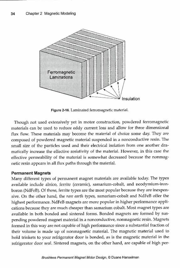
Figure 2-16. Laminated ferromagnetic material.

Though not used extensively yet in motor construction, powdered ferromagnetic materials can be used to reduce eddy current loss and allow for three dimensional flux flow. These materials may become the material of choice some day. They are composed of powdered magnetic material suspended in a nonconductive resin. The small size of the particles used and their electrical isolation from one another dra-matically increase the effective resistivity of the material. However, in this case the effective permeability of the material is somewhat decreased because the nonmag-netic resin appears in all flux paths through the material.

Permanent Magnets Many different types of permanent magnet materials are available today. The types available include alnico, ferrite (ceramic), samarium-cobalt, and neodymium-iron-boron (NdFeB). Of these, ferrite types are the most popular because they are inexpen-sive. On the other hand, the rare earth types, samarium-cobalt and NdFeB offer the highest performance. NdFeB magnets are more popular in higher performance appli-cations because they are much cheaper than samarium cobalt. Most magnet types are available in both bonded and sintered forms. Bonded magnets are formed by sus-pending powdered magnet material in a nonconductive, nonmagnetic resin. Magnets formed in this way are not capable of high performance since a substantial fraction of their volume is made up of nonmagnetic material. The magnetic material used to hold trinkets to your refrigerator door is bonded, as is the magnetic material in the refrigerator door seal. Sintered magnets, on the other hand, are capable of high per-

formance because the sintering process allows magnets to be formed without a bond-ing agent. Overall, each magnet type has different properties leading to different con-straints and different levels of performance in brushless permanent magnet motors. Rather than exhaustively discuss each of these magnet types, this text discusses only generic properties.

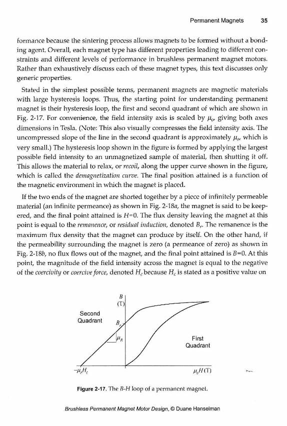
Stated in the simplest possible terms, permanent magnets are magnetic materials with large hysteresis loops. Thus, the starting point for understanding permanent magnet is their hysteresis loop, the first and second quadrant of which are shown in Fig. 2-17. For convenience, the field intensity axis is scaled by fi0, giving both axes dimensions in Tesla. (Note: This also visually compresses the field intensity axis. The uncompressed slope of the line in the second quadrant is approximately fi0, which is very small.) The hysteresis loop shown in the figure is formed by applying the largest possible field intensity to an unmagnetized sample of material, then shutting it off. This allows the material to relax, or recoil, along the upper curve shown in the figure, which is called the demagnetization curve. The final position attained is a function of the magnetic environment in which the magnet is placed.

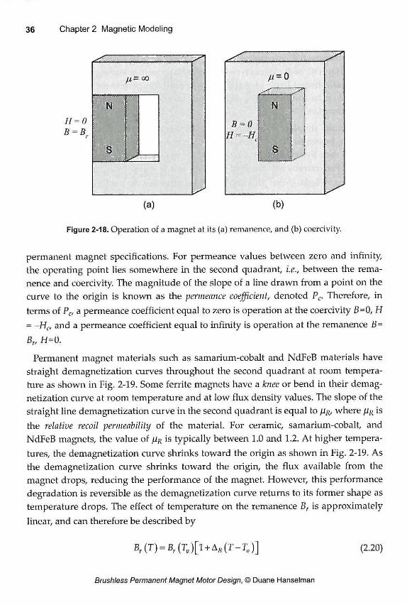
If the two ends of the magnet are shorted together by a piece of infinitely permeable material (an infinite permeance) as shown in Fig. 2-18a, the magnet is said to be keep-ered, and the final point attained is H=0. The flux density leaving the magnet at this point is equal to the remanence, or residual induction, denoted Br. The remanence is the maximum flux density that the magnet can produce by itself. On the other hand, if the permeability surrounding the magnet is zero (a permeance of zero) as shown in Fig. 2-18b, no flux flows out of the magnet, and the final point attained is B=0. At this point, the magnitude of the field intensity across the magnet is equal to the negative of the coercivity or coercive force, denoted Hc because Hc is stated as a positive value on

B

Figure 2-17. The B-H loop of a permanent magnet.

(a) (b)

Figure 2-18. Operation of a magnet at its (a) remanence, and (b) coercivity.

permanent magnet specifications. For permeance values between zero and infinity, the operating point lies somewhere in the second quadrant, i.e., between the rema-nence and coercivity. The magnitude of the slope of a line drawn from a point on the curve to the origin is known as the permeance coefficient, denoted Pc. Therefore, in terms of Pc, a permeance coefficient equal to zero is operation at the coercivity B~0, H = -Hc, and a permeance coefficient equal to infinity is operation at the remanence B= Br, H=0.

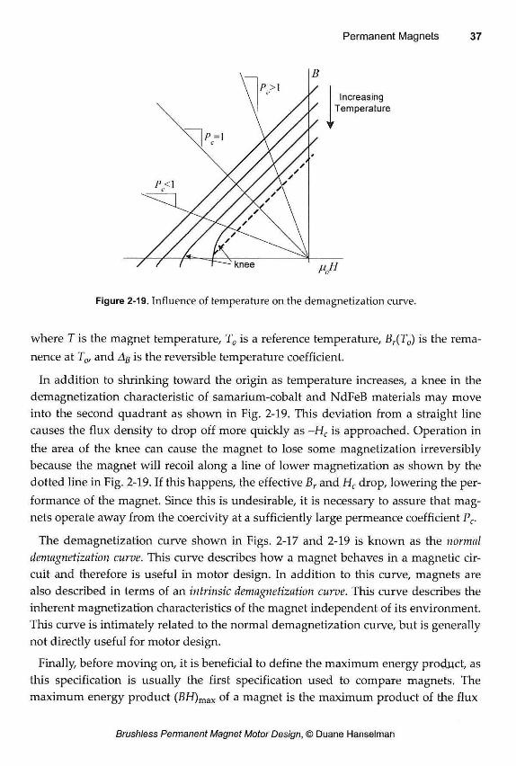
Permanent magnet materials such as samarium-cobalt and NdFeB materials have straight demagnetization curves throughout the second quadrant at room tempera-hire as shown in Fig. 2-19. Some ferrite magnets have a knee or bend in their demag-netization curve at room temperature and at low flux density values. The slope of the straight line demagnetization curve in the second quadrant is equal to jur, where /Jr is the relative recoil permeability of the material. For ceramic, samarium-cobalt, and NdFeB magnets, the value of fiR is typically between 1.0 and 1.2. At higher tempera-tures, the demagnetization curve shrinks toward the origin as shown in Fig. 2-19. As the demagnetization curve shrinks toward the origin, the flux available from the magnet drops, reducing the performance of the magnet. However, this performance degradation is reversible as the demagnetization curve returns to its former shape as temperature drops. The effect of temperature on the remanence Br is approximately linear, and can therefore be described by

Br(T)=Br(T0)[l + AB(T-T0)] (2.20)

/ Temperature

/ " /

B

Increasing

Figure 2-19. Influence of temperature ori the demagnetization curve.

where T is the magnet temperature, T0 is a reference temperature, Br(T0) is the rema-nence at T0, and A$ is the reversible temperature coefficient.

In addition to shrinking toward the origin as temperature increases, a knee in the demagnetization characteristic of samarium-cobalt and NdFeB materials may move into the second quadrant as shown in Fig. 2-19. This deviation from a straight line causes the flux density to drop off more quickly as -Hc is approached. Operation in the area of the knee can cause the magnet to lose some magnetization irreversibly because the magnet will recoil along a line of lower magnetization as shown by the dotted line in Fig. 2-19. If this happens, the effective Br and Hc drop, lowering the per-formance of the magnet. Since this is undesirable, it is necessary to assure that mag-nets operate away from the coercivity at a sufficiently large permeance coefficient Pc.

The demagnetization curve shown in Figs. 2-17 and 2-19 is known as the normal demagnetization curve. This curve describes how a magnet behaves in a magnetic cir-cuit and therefore is useful in motor design. In addition to this curve, magnets are also described in terms of an intrinsic demagnetization curve. This curve describes the inherent magnetization characteristics of the magnet independent of its environment. This curve is intimately related to the normal demagnetization curve, but is generally not directly useful for motor design.

Finally, before moving on, it is beneficial to define the maximum energy product, as this specification is usually the first specification used to compare magnets. The maximum energy product (BH)m a x of a magnet is the maximum product of the flux

density and field intensity along the magnet demagnetization curve. Even though this product has units of energy, it is not actual stored magnet energy, but rather it is a qualitative measure of a magnet's performance capability in a magnetic circuit. By convention, (BH)m a x is usually specified in the English units of millions of Gauss-Oer-steds (MG-Oe). However, some magnet manufacturers do conform to SI units of Joules per cubic meter (lMG-Oe=7.958 kj/m3). For magnets with /iR« 1, (BH)m a x

occurs near the unity permeance coefficient operating point. It can be shown that operation at (BH)m a x is the most efficient in terms of magnet volumetric energy den-sity. Despite this fact, permanent magnets in motors are almost never operated at (BH)max because of possible irreversible demagnetization with increasing tempera-ture as discussed in the previous paragraph.

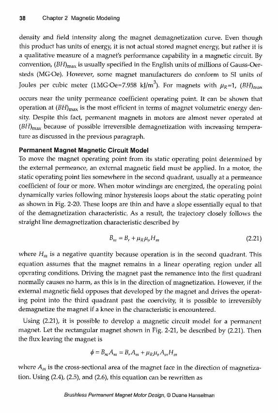
Permanent Magnet Magnetic Circuit Model To move the magnet operating point from its static operating point determined by the external permeance, an external magnetic field must be applied. In a motor, the static operating point lies somewhere in the second quadrant, usually at a permeance coefficient of four or more. When motor windings are energized, the operating point dynamically varies following minor hysteresis loops about the static operating point as shown in Fig. 2-20. These loops are thin and have a slope essentially equal to that of the demagnetization characteristic. As a result, the trajectory closely follows the straight line demagnetization characteristic described by

Bm=Br+WoHm (2.21)

where Hm is a negative quantity because operation is in the second quadrant. This equation assumes that the magnet remains in a linear operating region under all operating conditions. Driving the magnet past the remanence into the first quadrant normally causes no harm, as this is in the direction of magnetization. However, if the external magnetic field opposes that developed by the magnet and drives the operat-ing point into the third quadrant past the coercivity, it is possible to irreversibly demagnetize the magnet if a knee in the characteristic is encountered.

Using (2.21), it is possible to develop a magnetic circuit model for a permanent magnet. Let the rectangular magnet shown in Fig. 2-21, be described by (2.21). Then the flux leaving the magnet is

0 = BmAm = BrAm + ^ o A m H m

where Am is the cross-sectional area of the magnet face in the direction of magnetiza-tion. Using (2.4), (2.5), and (2.6), this equation can be rewritten as

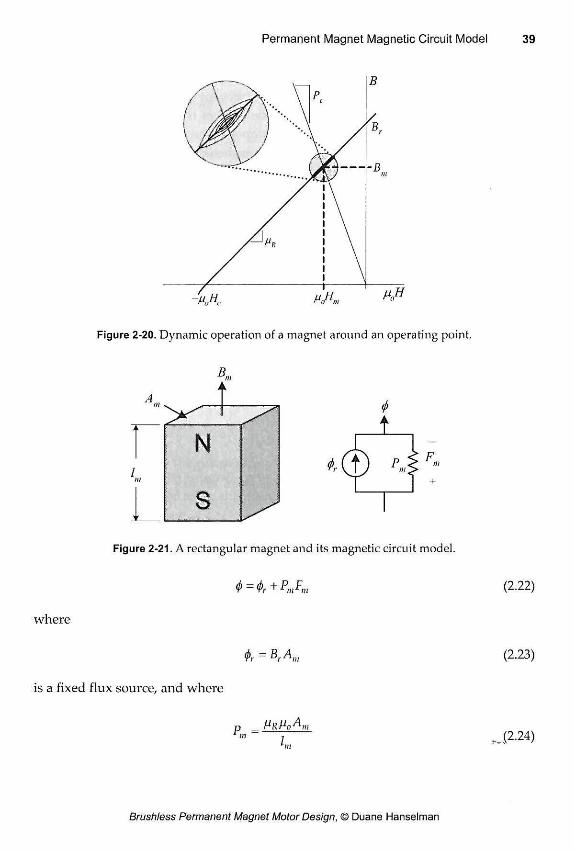
Permanent Magnet Magnetic Circuit Model 39

M0Hnl

Figure 2-20. Dynamic operation of a magnet around an operating point.

where

1 F.

Figure 2-21. A rectangular magnet and its magnetic circuit model.

= <i>r+P,nFnl (2.22)

K = BrAm

is a fixed flux source, and where

P.„ = PrPoAT

(2.23)

,,.(2-24)

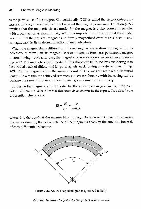
is the permeance of the magnet. Conventionally (2.24) is called the magnet leakage per-meance, although here it will simply be called the magnet permeance. Equation (2.22) implies that the magnetic circuit model for the magnet is a flux source in parallel with a permeance as shown in Fig. 2-21. It is important to recognize that this model assumes that the physical magnet is uniformly magnetized over its cross section and is magnetized in its preferred direction of magnetization.

When the magnet shape differs from the rectangular shape shown in Fig. 2-21, it is necessary to reevaluate its magnetic circuit model In brushless permanent magnet motors having a radial air gap, the magnet shape may appear as an arc as shown in Fig. 2-22. The magnetic circuit model of this shape can be found by considering it to be a radial stack of differential length magnets, each having a model as given in Fig. 2-21. During magnetization the same amount of flux magnetizes each differential length. As a result, the achieved remanence decreases linearly with increasing radius because the same flux over a increasing area gives a smaller flux density.

To derive the magnetic circuit model for the arc-shaped magnet in Fig. 2-22, con-sider a differential slice of radial thickness dr as shown in the figure. This slice has a differential reluctance of

where L is the depth of the magnet into the page. Because reluctances add in series just as resistors do, the net reluctance of the magnet is given by the sum, i.e., integral, of each differential reluctance

dR = = /uA ßrOmL

= dl = dr

•dr

Figure 2-22. An arc-shaped magnet magnetized radially.

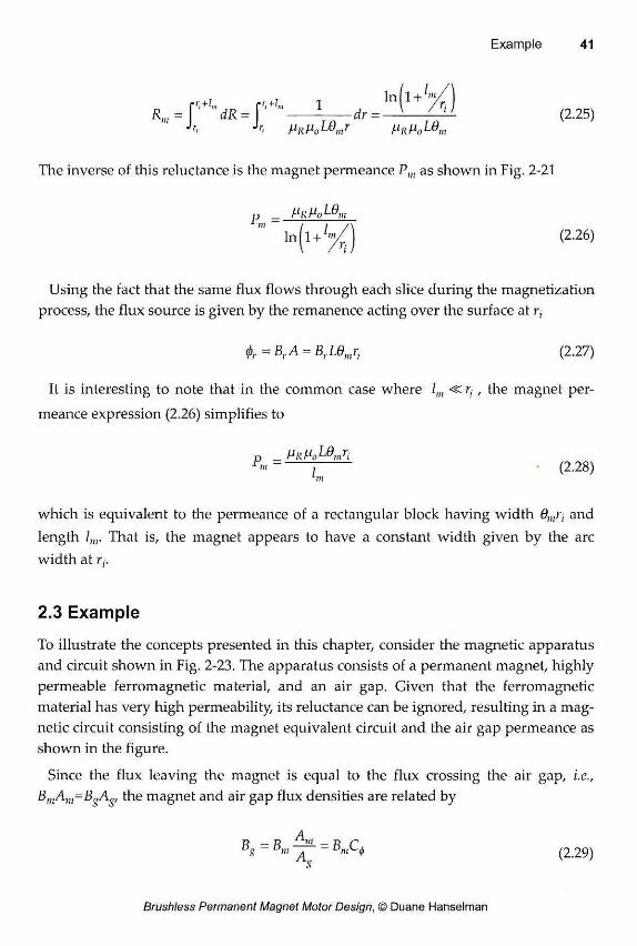
Jr, Jr, f.lRH0L9mr /-IrVo10»,

The inverse of this reluctance is the magnet permeance Pm as shown in Fig. 2-21

ln(l + ) (2.26) P.„ =

Using the fact that the same flux flows through each slice during the magnetization process, the flux source is given by the remanence acting over the surface at r,

<j)r = Br A = B,.L9mri (2.27)

It is interesting to note that in the common case where l m <s: r,, the magnet per-

meance expression (2.26) simplifies to

_ HR»0lAmri 1 ~ 7 (2.28)

Lm which is equivalent to the permeance of a rectangular block having width 9mr{ and length /,„. That is, the magnet appears to have a constant width given by the arc width at rv

2.3 Example

To illustrate the concepts presented in this chapter, consider the magnetic apparatus and circuit shown in Fig. 2-23. The apparatus consists of a permanent magnet, highly permeable ferromagnetic material, and an air gap. Given that the ferromagnetic material has very high permeability, its reluctance can be ignored, resulting in a mag-netic circuit consisting of the magnet equivalent circuit and the air gap permeance as shown in the figure.

Since the flux leaving the magnet is equal to the flux crossing the air gap, i.e., BmA„i=BgAs, the magnet and air gap flux densities are related by

Bx = B»> = B»'C4> (2.29)

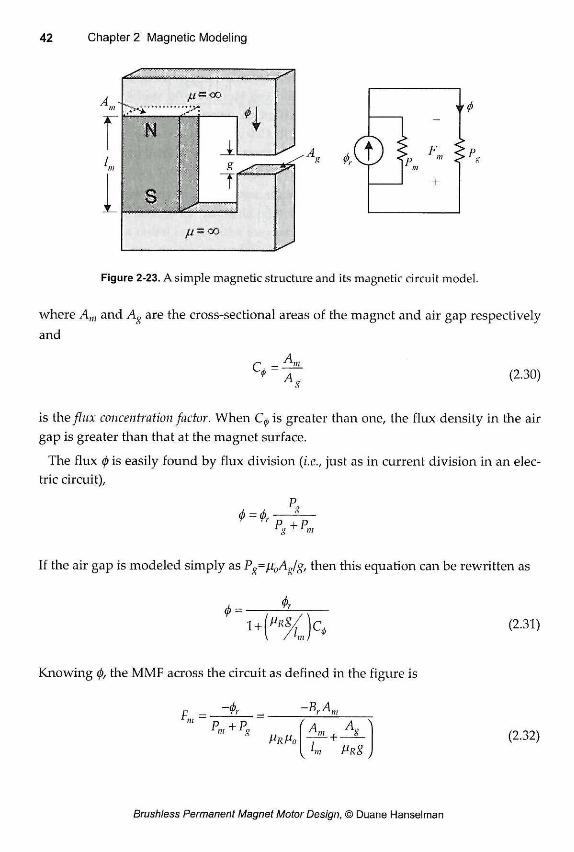
F >p in ' „

Figure 2-23. A simple magnetic structure and its magnetic circuit model.

where Am and Ag are the cross-sectional areas of the magnet and air gap respectively and

r -(2.30)

is the flux concentration factor. When Cq is greater than one, the flux density in the air gap is greater than that at the magnet surface.

The flux 0 is easily found by flux division (i.e., just as in current division in an elec-tric circuit),

'' P +P 1 g ^1 m

If the air gap is modeled simply as Pg=/i0As/g, then this equation can be rewritten as

(2.31)

Knowing 0, the MMF across the circuit as defined in the figure is

F.= ~<t>, ~BrAr

P +P 1 m ^ 1 g PrMO

L PRg (2.32)

These two equations describe the flux and MMF solutions of the magnetic circuit. As stated, the two equations do not provide any significant insight into the operation of the circuit. There are simply too many variables in the equations.

However, recognizing that Bm=<f)/Am and Hm=Fm/lm, the permeance coefficient defining the operating point is given by

p _ ~B"> _ lm 1

This remarkably simple result says that the ratio of the magnet length to the air gap length and the flux concentration factor determine the permeance coefficient. Since the permeance coefficient must be greater than one for safe operation of the magnet especially at higher temperatures, the magnet length must be significantly larger than the air gap length. Moreover, any attempt to increase the air gap flux density through flux concentration, i.e., C<p> 1, pushes the permeance coefficient lower.

The fundamental importance of (2.33) can be seen by considering what is required to maintain a constant permeance coefficient as the flux concentration factor increases. Multiplying the numerator and denominator of (2.33) by A m A s and simpli-fying gives

p

• ~ C j (2-34>

where Vm and V are the magnet and air gap volumes respectively. Now if C is dou-bled to 2C^ and the air gap volume remains constant, the magnet volume must

increase by a factor of 2 =4 to maintain a constant permeance coefficient. If the mag-net cross-sectional area remains constant, this implies that the magnet length must increase by a factor of 4. The implication of this analysis is that concentrating the flux of a permanent magnet comes with the penalty of geometrically increasing magnet volume.

2.4 Summary

In this chapter, the basics of magnetic circuit analysis were presented. Starting with fundamental magnetic field concepts, the concepts of permeance, reluctance, flux, and MMF were developed. Permeance models for blocks of magnetic material, air gaps and slotted magnetic structures were developed. The properties of ferromag-

netic and permanent magnet materials were discussed. A magnetic circuit model of a permanent magnet was introduced and the concept of flux concentration was illus-trated.

With this background it is now possible to discuss how magnetic fields interact with the electrical and mechanical parts of a motor. These concepts are discussed in the next chapter.

As stated in the first chapter, the operation of a brushless permanent magnet motor relies on the conversion of electrical energy to magnetic energy and from magnetic energy to mechanical energy. In this chapter, the connections between magnetic field concepts, electrical circuits, and mechanical motion will be explored to illustrate this energy conversion process.

3.1 Flux Linkage and Inductance

Self Inductance To define flux linkage and self inductance, consider the magnetic circuit shown in Fig. 3-1. This circuit is said to be singly excited since it has only one coil to produce a magnetic field. The flux (p flowing around the core is due to the current i and the direction of flux flow is clockwise because of the right hand rule. Using the magnetic circuit equivalent of Ohm's law, the flux produced is given by

where R is the reluctance seen by the MMF source. Since this flux passes through, or links, all N turns of the winding, the total flux linked by the winding is called the flux linkage, which is defined as

This expression shows that flux linkage is directly proportional to coil current. As a result, it is common to define the constant relating current to flux linkage as induc-tance

A = N<f> (3.2)

Combining these two equations gives

(3.3)

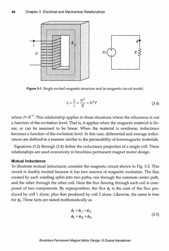
N

—'

O R

Figure 3-1. Single excited magnetic structure and its magnetic circuit model.

J = ~ R = M

where P=R \ This relationship applies in those situations where the reluctance is not a function of the excitation level. That is, it applies when the magnetic material is lin-ear, or can be assumed to be linear. When the material is nonlinear, inductance becomes a function of the excitation level. In this case, differential and average induc-tances are defined in a manner similar to the permeability of ferromagnetic materials.

Equations (3.2) through (3.4) define the inductance properties of a single coil. These relationships are used extensively in brushless permanent magnet motor design.

Mutual Inductance To illustrate mutual inductance, consider the magnetic circuit shown in Fig. 3-2. This circuit is doubly excited because it has two sources of magnetic excitation. The flux created by each winding splits into two paths, one through the common center path, and the other through the other coil. Here the flux flowing through each coil is com-posed of two components. By superposition, the flux fa is the sum of the flux pro-duced by coil 1 alone, plus that produced by coil 2 alone. Likewise, the same is true for 02- These facts are stated mathematically as

02=022+021

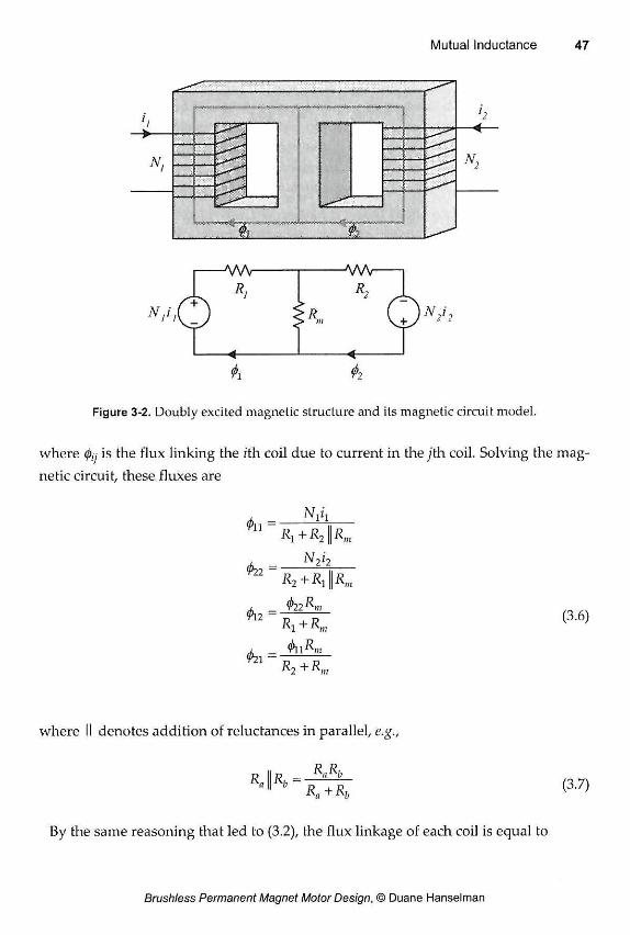
N ,i •O R,

•A/W

R © N2i2

Figure 3-2. Doubly excited magnetic structure and its magnetic circuit model.

where (p,j is the flux linking the ¿th coil due to current in the y'th coil. Solving the mag-netic circuit, these fluxes are

0n =

022 =

012 =

021 =

Nlh Ri+Ri K <t>nK

R1 + Rm

011 Rt+R,„

(3.6)

where II denotes addition of reluctances in parallel, e.g.,

Ä J J ^ J ^ L . (3.7)

By the same reasoning that led to (3.2), the flux linkage of each coil is equal to

¿2 =N 2 0 2 =N2(022+02]) (3.8)

Combining the above expressions leads to

Àq — jLjî-J + L n Ì 2

À2 = ¿21 + ¿2 '2

where the self inductances, Lj and L2, are

(3.9)

L M -

zi .

N

,2=o

u =

„=0

(3.10)

and the mutual inductances are

L -h. L12 - . h

-L -h, - l 2 1 - . /,= 0

N,N2RIU

h=0 R^+R^+R^ (3.11)

The self inductance expressions in (3.10) are identical to (3.4) in that the denomina-tors in (3.10) are equal to the reluctance seen by the respective coils. The mutual inductance (3.11) is due to the mutual coupling between the two coils. The reluctance Rm governs the mutual inductance. If Rm is zero, both coils see a magnetic short through the center path and no flux from either coil is linked to the other. Setting Rni

to zero in (3.11) confirms this, as the mutual inductance is zero in this case. On the other hand, if Rm goes to infinity (a magnetic open circuit), the entire flux from each coil is coupled to the other, since there is no other flux path except that through the other coil. In this case, the mutual inductance is maximum and equal to (L\L2 )1 / 2 .

Mutually coupled coils appear in most brushless permanent magnet motors. Motors typically have two or more phases, each composed of one or more coils. As a general rule, the self inductance of the phase windings is usually much greater than the mutual inductance between windings. In this case, the above derivation is easily generalized to include the mutual inductances between all pairs of coils.

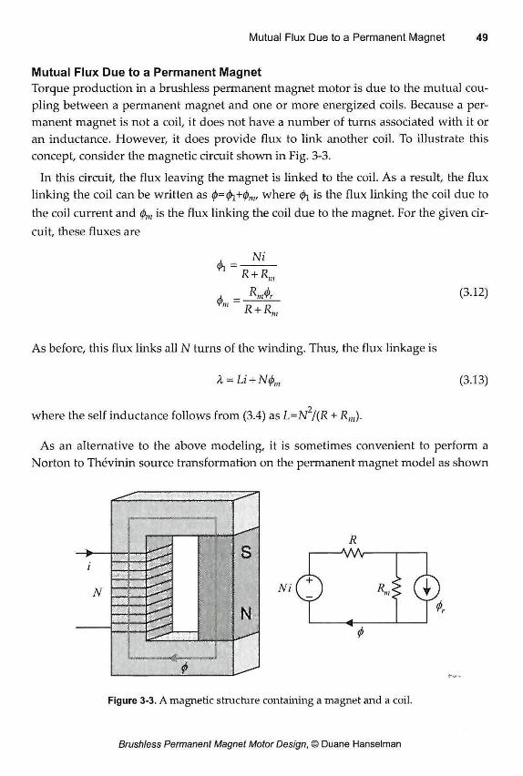
Mutual Flux Due to a Permanent Magnet 49

Mutual Flux Due to a Permanent Magnet Torque production in a brushless permanent magnet motor is due to the mutual cou-pling between a permanent magnet and one or more energized coils. Because a per-manent magnet is not a coil, it does not have a number of turns associated with it or an inductance. However, it does provide flux to link another coil. To illustrate this concept, consider the magnetic circuit shown in Fig. 3-3.

In this circuit, the flux leaving the magnet is linked to the coil. As a result, the flux linking the coil can be written as 0=0i+(pm, where (pi is the flux linking the coil due to the coil current and (f>m is the flux linking the coil due to the magnet. For the given cir-cuit, these fluxes are

0i = Ni

R + Rm

_ Kb R + R„

(3.12)

As before, this flux links all N turns of the winding. Thus, the flux linkage is

X-Li + N(j)m (3.13)

where the self inductance follows from (3.4) as L=N /(R + Rm).

As an alternative to the above modeling, it is sometimes convenient to perform a Norton to Thévinin source transformation on the permanent magnet model as shown

ßä

l

N

-—

S R

-AAV

"'O © t

Figure 3-3. A magnetic structure containing a magnet and a coil.

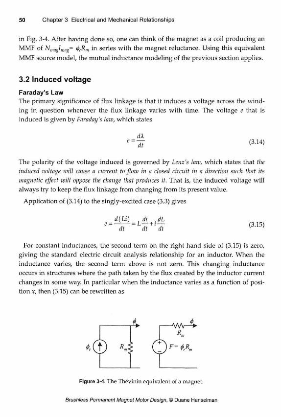
in Fig. 3-4. After having done so, one can think of the magnet as a coil producing an MMF of N i mgln l n g= (¡)rRm in series with the magnet reluctance. Using this equivalent MMF source model, the mutual inductance modeling of the previous section applies.

3.2 Induced voltage

Faraday's Law The primary significance of flux linkage is that it induces a voltage across the wind-ing in question whenever the flux linkage varies with time. The voltage e that is induced is given by Faraday's law, which states

e = ctt dt (3.14)

The polarity of the voltage induced is governed by Lenz's lazv, which states that the induced voltage will cause a current to flow in a closed circuit in a direction such that its magnetic effect will oppose the change that produces it. That is, the induced voltage will always try to keep the flux linkage from changing from its present value.

Application of (3.14) to the singly-excited case (3.3) gives

d(Li) di .dl e = ——- = L— + i —

dt dt dt (3.15)

For constant inductances, the second term on the right hand side of (3.15) is zero, giving the standard electric circuit analysis relationship for an inductor. When the inductance varies, the second term above is not zero. This changing inductance occurs in structures where the path taken by the flux created by the inductor current changes in some way. In particular when the inductance varies as a function of posi-tion x, then (3.15) can be rewritten as

Q F= ¿A

Figure 3-4. The Thévinin equivalent of a magnet.

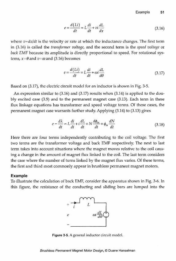
d(Li) T di .dL e — = L 7 t + m T * <3-16>

where v=dx/dt is the velocity or rate at which the inductance changes. The first term in (3.16) is called the transformer voltage, and the second term is the speed voltage or back EMF because its amplitude is directly proportional to speed. For rotational sys-tems, x=0and u=iwand (3.16) becomes

d(Li) di .dL e = ——- = L—+cot— (3.17)

dt dt d6 K '

Based on (3.17), the electric circuit model for an inductor is shown in Fig. 3-5.

An expression similar to (3.16) and (3.17) results when (3.14) is applied to the dou-bly excited case (3.9) and to the permanent magnet case (3.13). Each term in these flux linkage equations has transformer and speed voltage terms. Of these cases, the permanent magnet case warrants further study. Applying (3.14) to (3.13) gives

dl _ di .dL d(j)m , dN

Here there are four terms independently contributing to the coil voltage. The first two terms are the transformer voltage and back EMF respectively. The next to last term takes into account situations where the magnet moves relative to the coil caus-ing a change in the amount of magnet flux linked to the coil. The last term considers the case where the number of turns linked by the magnet flux varies. Of these terms, the first and third most commonly appear in brushless permanent magnet motors.

Example To illustrate the calculation of back EMF, consider the apparatus shown in Fig. 3-6. In this figure, the resistance of the conducting and sliding bars are lumped into the

i . dL /"+N

Figure 3-5. A general inductor circuit model.

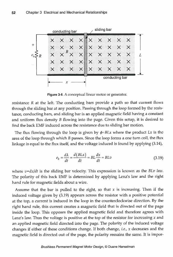
conducting bar sliding bar

X X X X " x X X X X + X X X

x * x

X X X X X X

*A< >R X X X x * x X : X X X X X

X X x X X X X X X X X X X X X X X X

conducting bar

Figure 3-6. A conceptual linear motor or generator.

resistance R at the left. The conducting bars provide a path so that current flows through the sliding bar at any position. Passing through the loop formed by the resis-tance, conducting bars, and sliding bar is an applied magnetic field having a constant and uniform flux density B flowing into the page. Given this setup, it is desired to find the back EMF induced across the resistance due to sliding bar motion.

The flux flowing through the loop is given by <f>=BLx where the product Lx is the area of the loop through which B passes. Since the loop forms a one turn coil, the flux linkage is equal to the flux itself, and the voltage induced is found by applying (3.14),

dt dt dt (3.19)

where v=dx/dt is the sliding bar velocity. This expression is known as the BLv law. The polarity of this back EMF is determined by applying Lenz's law and the right hand rule for magnetic fields about a wire.

Assume that the bar is pulled to the right, so that x is increasing. Then if the induced voltage given by (3.19) appears across the resistor with a positive potential at the top, a current is induced in the loop in the counterclockwise direction. By the right hand rule, this current creates a magnetic field that is directed out of the page inside the loop. This opposes the applied magnetic field and therefore agrees with Lenz's law. Thus the voltage is positive at the top of the resistor for increasing x and an applied magnetic field directed into the page. The polarity of the induced voltage changes if either of these conditions change. If both change, i.e., x decreases and the magnetic field is directed out of the page, the polarity remains the same. It is impor-

Energy and Coenergy in Singly-Excited Systems 53

tant to note that the magnetic field produced by current in the loop does not modify B in (3.19). Equation (3.19) is independent of the magnetic field produced by current flow.

Operation of this structure can also be understood from an energy perspective. Mechanical energy input from the sliding bar creates electrical energy that is con-verted to heat by the resistor. Although the BLv law is derived for the apparatus shown in Fig. 3-6, it is useful in many applications where a constant flux density passes through a coil. In particular, it is useful for brushless permanent magnet motor design.

3.3 Energy and Coenergy

The energy stored in a magnetic field is an important quantity to know in the design and analysis of brushless permanent magnet motors, as the magnetic field is the medium through which electric energy is converted to mechanical energy. In addi-tion, knowing the energy or coenergy stored in a magnetic field provides one method for computing inductance.

Energy and Coenergy in Singly-Excited Systems To illustrate the computation of energy and coenergy, reconsider the singly-excited magnetic circuit shown in Fig. 3-1. If one ignores resistive losses, the instantaneous power delivered to the magnetic field of the coil is p-ei where e and i are the instanta-neous voltage and current respectively in the coil forming the MMF source. Using (3.14), this can be rewritten as

Since power is the rate at which energy is transmitted, the energy stored in the coil at a time t is given by the integral of power

where A(0) is the initial flux linkage and A(t) is the flux linkage at time t. For a linear magnetic circuit, i and A are related by the inductance given in (3.4).

Substituting (3.4) into the above expression gives

.dX_ (3.20)

(3.21)

(3.22)

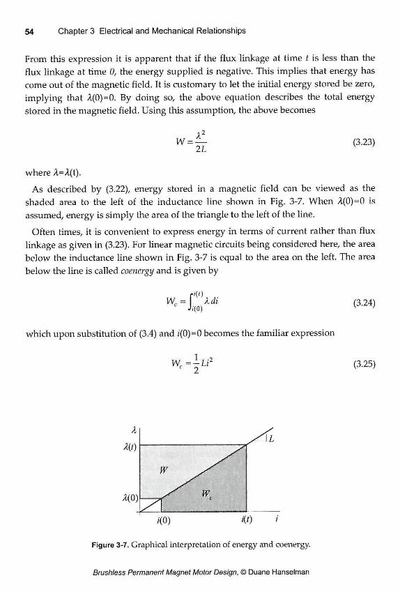
From this expression it is apparent that if the flux linkage at time t is less than the flux linkage at time 0, the energy supplied is negative. This implies that energy has come out of the magnetic field. It is customary to let the initial energy stored be zero, implying that A(0)=0. By doing so, the above equation describes the total energy stored in the magnetic field. Using this assumption, the above becomes

where A=A(t).

As described by (3.22), energy stored in a magnetic field can be viewed as the shaded area to the left of the inductance line shown in Fig. 3-7. When A(0)=0 is assumed, energy is simply the area of the triangle to the left of the line.

Often times, it is convenient to express energy in terms of current rather than flux linkage as given in (3.23). For linear magnetic circuits being considered here, the area below the inductance line shown in Fig. 3-7 is equal to the area on the left. The area below the line is called coenergy and is given by

rf(')

W c = \ i m X d i (3.24)

which upon substitution of (3.4) and z(0)=0 becomes the familiar expression W C =ÌL/ 2 (3.25)

Energy and Coenergy in Doubly-Excited Systems 55

Equations (3.23) and (3.25) define the energy and coenergy stored in a singly-excited magnetic circuit. Before considering doubly-excited circuits, it is useful to express energy and coenergy in terms of magnetic circuit and magnetic field parame-ters. Since P=fiA/l, L=N2P, and F=Ni, energy and coenergy can be written respectively as

2 j 2

2L 2 (N2P) 2P i 1 i (3.26)

Wc = - U 2 = - ( N 2 P ) i 2 = -PF2

C 2 2 \ ) 2

in terms of magnetic circuit parameters. In these equations P, and F are the flux, permeance, and MMF associated with the coil forming the inductance L.

These expressions can be related to the magnetic field parameters B, H and ¡1 to express energy and coenergy per unit volume. Since <p=BA, F=Hl, and volume is Al, (3.26) can be manipulated to give the energy and coenergy densities

W <j>2 (BA)2 B2

iv = Al IP Al 2^A/jAl

c Al 2AI 2 Al

(3.27)

Energy and Coenergy in Doubly-Excited Systems For doubly-excited systems such as that shown in Fig. 3-2, expressions for energy and coenergy are more involved because energy is stored in both the self and mutual inductances. In particular, the calculation of energy stored in mutual inductance requires more rigor than the preceding analysis. As a result, only the final result is given here and the interested reader is encouraged to consult other references.

The instantaneous power delivered to the magnetic field in Fig. 3-2 is

. dXi . dXj p^-g+^it (3-28)

where the subscripts refer to the respective coils and currents are expressed iri lower case characters. From this expression, the energy stored in the magnetic field is

,2 12 W = i l l - + +^12^21,

2L-[ L\2 (3.29)

where A1 1=N10n , Ai2=Ni0i2 a n d The coenergy follows as

Lrf + i L2i*2 + hhUi (3.30)

A comparison of (3.29) and (3.30) shows the apparent advantage of using coenergy, as the terms in (3.30) are much more obvious. In these equations, the first two terms are the energy and coenergy stored in the self inductances respectively, and the last term is energy and coenergy stored in the mutual inductance.

Coenergy in the Presence of a Permanent Magnet Because of its importance in brushless permanent magnet motors, it is important to consider the coenergy stored in the magnetic field of a magnetic circuit containing a permanent magnet. For the magnetic circuit shown in Fig. 3-3, the coenergy stored is

Wc = U t 2 + ^ ( R + R m ) t i l + Ni<i>m (3.31)

where (j)m is the magnet flux linking the coil. In this expression, the first term is the coenergy stored in the self inductance, the second term is the coenergy stored due to the magnet alone, and the last is the coenergy due to mutual flux. As will be dis-cussed next, the torque produced by a motor is composed of two components, one due to the self inductance terms in (3.31) and the other due to the mutual terms. In a brushless permanent magnet motor, the torque due to mutual terms is desired and that due to self inductance terms is commonly parasitic.

3.4 Force, Torque and Power

The torque produced by a brushless permanent magnet motor is the most important quantity to be determined. Torque is a measure of the turning force that can be pro-duced in a motor and represents the fundamental specification to be met in all appli-cations.

Basic Relationships Energy in a mechanical system is called work. Work is equal to the product of force and distance. More accurately it is the product of the displacement of an object and the component of the force along the direction of displacement. Thus a differential

Force, Torque and Power 57

amount of mechanical energy can be written as dWm=Fdx where Wm is mechanical energy, F is the force in the x direction, and dx is a differential length in the x direc-tion.

Power is the amount of work done per unit time, or the time rate of change of energy. Thus, from the above, mechanical power is given by

dWm _pdx dt dt

P„,= — - F—-Fv (3.32)

where v is the velocity of motion.

When motion is confined to rotation, one deals with torque rather than force. The relationship between torque and force was discussed earlier in Chapter 1 and is described in Fig. 1-4 and by (1.1). A tangential force F, acting at a radius r, produces a torque T, given by the product of the force and the length of the lever arm r over which the force is acting, i.e., T=Fr . In this case, a differential amount of work is given by dWm=Fdx=FrdO=Tdd where the relationship between circumferential dis-tance and angular position x=r6 has been used. Finally, as defined earlier, the mechanical power is

dwnL^Tde_ dt dt R..= —-T — = Tco (3.33)

where CO is the rotational speed in mechanical radians per second, radM/s.

Fundamental Implications

Equations (1.8) and (3.33) play an important role in the design of motors. Since torque is proportional to diameter squared as stated in (1.8) and since by (3.33) power is directly proportional to torque, a motor having a larger diameter at which torque is generated will produce more mechanical power. Therefore it appears that motor diameter should be maximized. However, there are a number of constraints that limit the diameter of a motor. The most obvious constraint is the physical space limitations dictated by a particular application. Other constraints are volume, mass, and inertia. The volume of a motor increases with the square of radius or diameter. Thus, the ratio of output power to volume cannot be increased by increasing motor diameter. Since motor mass is proportional to its volume, the ratio of output power to mass cannot be increased either, unless the average mass density of the motor vol-ume decreases as diameter increases. As diameter increases, it is usually possible to have an increasing proportion of the motor volume be composed of air. Therefore, some increase in power density is possible as diameter increases. The last constraint,

inertia, is significant in applications requiring maximum torque to inertia ratio. The inertia of a rotor is proportional to the fourth power of its radius or diameter. There-fore, the torque to inertia ratio of a motor decreases as the square of rotor radius. Clearly, in cases where the inertia is to be minimized, a large diameter must be avoided.

Besides the significance of diameter, (1.8) and (3.33) indicate several other impor-tant points. Once a diameter is chosen, there are two ways to increase the power developed. The first is to increase the speed at which the motor operates. In most applications, the load speed is specified; therefore the only way to increase power by increasing speed is to use some form of speed reduction between the motor and its load. While this is simple conceptually, speed reduction components add significant volume, mass, inertia, cost, frictional losses, and reduced reliability that must be weighed against the benefits of higher speed operation. The other way to increase power for a fixed diameter is to increase the force density acting on the rotor. This is accomplished by increasing the electrical and magnetic operating points of the motor. Often these are referred to as the electric and magnetic loadings respectively. Again, this does not come without constraints. Increasing the electrical operating point implies increasing the current supplied to the motor. This adds ohmic I R loss to the system that increases as the square of current and that must be removed from the system. In a brushless permanent magnet motor, increasing the magnetic field oper-ating point requires more or higher performance magnet material, or specialized motor construction to focus or concentrate flux into the air gap. As was discussed earlier, flux concentration geometrically increases the amount of magnet material required. Moreover, additional ferromagnetic material is required to concentrate flux. Both of these increase the mass and volume of a motor.

It should be clear from the above discussion that getting the highest performance out of a motor for the least cost is not simple. When high performance is required, many physical constraints are pushed to their limits. As a result, high performance motor design requires that all physical constraints be identified and included in the design process. Engineering practice suggests that any constraint not included in the design process will likely be pushed well beyond what is feasible.

Torque From a Macroscopic Viewpoint There are two general ways to determine the torque produced by a magnetic field. The first of these is based on taking a macroscopic viewpoint, a viewpoint that uses the concept of conservation of energy. This method requires that all electrical, mag-netic, and mechanical losses in the motor be modeled as being external to the motor. What remains is a conservative system where no energy is lost. Any added electrical

Torque From a Macroscopic Viewpoint 59

energy must contribute to the energy stored in the magnetic field and to the output mechanical energy. Stated in terms of a differential amount of added energy, conser-vation of energy requires that dWe=dW + dWm where dWer dW, and dWm are differen-tial amounts of electrical, magnetic, and mechanical energies respectively.

Based on the above expression, it is possible to show that the torque can be related to the rate of change of field energy as

T = ~dW

de

and can be related to the rate of change of field coenergy as

(3.34) A=cunstant

T=dW" dd (3.35)

i=constant

The derivation of (3.34) and (3.35) can be found in many references, and the inter-ested reader is encouraged to refer to them. As stated above, positive torque acts to decrease the stored energy at constant flux, and acts to increase coenergy stored at constant current.

Equations (3.34) and (3.35) apply to the general case. When restricted to the linear case, these equations can be simplified. In addition, because coenergy is described in terms of current rather than flux linkage, (3.35) is the most convenient expression to use. Since both equations give the same result when appropriate substitutions are made, only results using (3.35) will be given here.

Application of (3.35) to the mutual inductance case (3.30) gives

1 ,2 ^ 1 .2 dh2 dlq2

The significance of this equation is best discussed by considering each term individu-ally. To do so, first assume that the system under investigation is singly excited, i.e., ¿2=0. In this case only the first term in (3.36) remains. The first term implies that the torque produced is a function of the square of the applied current, and therefore is not a function of the direction of current flow. This makes sense since an electromag-net will attract a piece of steel irrespective of the direction of current flow. In addi-tion, the first term implies that positive torque, or attraction, occurs whenever induc-tance is increasing. In other words, this torque term always acts to increase induc-

2 tance or permeance (since L=N P) and acts to decrease reluctance. As a result, this

term is called reluctance torque. The electromagnet example shows that this fact makes sense also, because the coil inductance and permeance of the magnetic circuit increase as the piece of steel is attracted closer to the electromagnet.

Next, if one assumes that ^=0, rather than i2 as considered above, only the second term in (3.36) remains. Because of the similarity between the first and second terms, this torque term is also reluctance torque and has the same properties as the first term.

Finally, if the self inductances Lt and L2 are both constant, only the last term in (3.36) remains. This term is due to the mutual flux or inductance between the two coils and is commonly called the mutual torque or alignment torque. This term exists only if there is some variation in the mutual inductance between the two coils. In this case, positive torque acts to increase the mutual coupling between the two coils when the currents have the same sign, and acts to decrease it when the currents have the opposite signs. With reference to Fig. 3-2, positive torque is produced when the mutual fluxes add, and negative torque is produced when the mutual fluxes oppose each other. Alternatively, this property states the well known axiom that opposite magnetic poles attract and like poles repel.

Application of (3.35) to the case of a mutually coupled coil and permanent magnet, (3.31) gives

^ 1 .2dl 1,2 dR ...d<p T = — r f— + (3.37)

2 d0 2 dO d6 K '

In this expression, the first two terms are the reluctance torque associated with the coil and magnet respectively, and the third term is the alignment torque due to the mutual flux 0 linking the magnet to the coil. The first term is identical to that in (3.36). The second term is a torque component proportional to the square of the flux leaving the magnet and is not a function of the polarity of the flux. The reason for the minus sign in front of this term is that inductance is inversely proportional to reluc-tance. Thus, dL/d6 is proportional to -dR/dQ, making the first and second terms in (3.37) equivalent in terms of torque production. Since the mutual flux linkage between the flux leaving the magnet (j) and the coil is A,„=N0, the last term in (3.37) is equivalent to the last term in (3.36) where Xn-Lnh

In a brushless permanent magnet motor, the first term in (3.37) appears when motor construction causes the winding inductance to vary as a function of position. The second term describes cogging torque that appears whenever magnet flux travels through a varying reluctance. The final term describes the mutual torque that is used

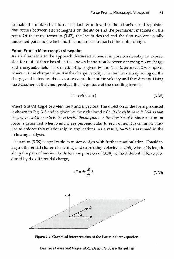
Force From a Microscopic Viewpoint 61

to make the motor shaft turn. This last term describes the attraction and repulsion that occurs between electromagnets on the stator and the permanent magnets on the rotor. Of the three terms in (3.37), the last is desired and the first two are usually undesired parasitics, which must be minimized as part of the motor design.

Force From a Microscopic Viewpoint As an alternative to the approach discussed above, it is possible develop an expres-sion for mutual force based on the known interaction between a moving point charge and a magnetic field. This relationship is given by the Lorentz force equation F=qvxB, where q is the charge value, v is the charge velocity, B is the flux density acting on the charge, and x denotes the vector cross product of the velocity and flux density. Using the definition of the cross product, the magnitude of the resulting force is

F = qvBsirx(a) (3.38)

where a is the angle between the v and B vectors. The direction of the force produced is shown in Fig. 3-8 and is given by the right hand rule: If the right hand is held so that the fingers curl from v to B, the extended thumb points in the direction of F. Since maximum force is generated when v and B are perpendicular to each other, it is common prac-tice to enforce this relationship in applications. As a result, a=n/2 is assumed in the following analysis.

Equation (3.38) is applicable to motor design with further manipulation. Consider-ing a differential charge element dq and expressing velocity as dl/dt, where / is length along the path of motion, leads to an expression of (3.38) as the differential force pro-duced by the differential charge,

Figure 3-8. Graphical interpretation of the Lorentz force equation.

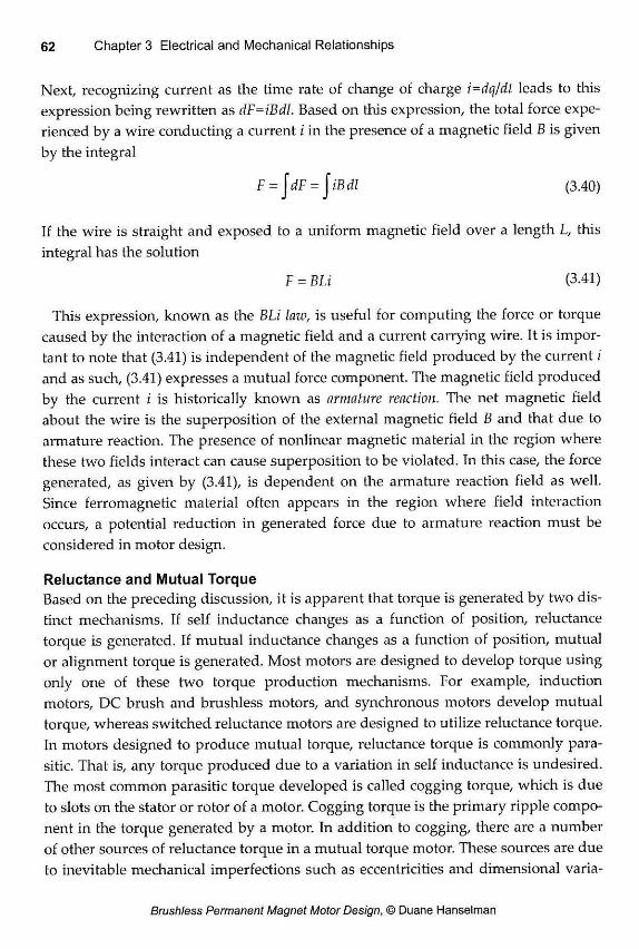
Next, recognizing current as the time rate of change of charge i=dq/dt leads to this expression being rewritten as dF=iBdl. Based on this expression, the total force expe-rienced by a wire conducting a current i in the presence of a magnetic field B is given by the integral

If the wire is straight and exposed to a uniform magnetic field over a length L, this integral has the solution

This expression, known as the BLi law, is useful for computing the force or torque caused by the interaction of a magnetic field and a current carrying wire. It is impor-tant to note that (3.41) is independent of the magnetic field produced by the current i and as such, (3.41) expresses a mutual force component. The magnetic field produced by the current i is historically known as armature reaction. The net magnetic field about the wire is the superposition of the external magnetic field B and that due to armature reaction. The presence of nonlinear magnetic material in the region where these two fields interact can cause superposition to be violated. In this case, the force generated, as given by (3.41), is dependent on the armature reaction field as well. Since ferromagnetic material often appears in the region where field interaction occurs, a potential reduction in generated force due to armature reaction must be considered in motor design.

Reluctance and Mutual Torque Based on the preceding discussion, it is apparent that torque is generated by two dis-tinct mechanisms. If self inductance changes as a function of position, reluctance torque is generated. If mutual inductance changes as a function of position, mutual or alignment torque is generated. Most motors are designed to develop torque using only one of these two torque production mechanisms. For example, induction motors, DC brush and brushless motors, and synchronous motors develop mutual torque, whereas switched reluctance motors are designed to utilize reluctance torque. In motors designed to produce mutual torque, reluctance torque is commonly para-sitic. That is, any torque produced due to a variation in self inductance is undesired. The most common parasitic torque developed is called cogging torque, which is due to slots on the stator or rotor of a motor. Cogging torque is the primary ripple compo-nent in the torque generated by a motor. In addition to cogging, there are a number of other sources of reluctance torque in a mutual torque motor. These sources are due to inevitable mechanical imperfections such as eccentricities and dimensional varia-

(3.40)

F = BLi (3.41)

tions. Since constant torque is usually desired from, a motor to produce smooth mechanical motion, parasitic torque components must be minimized.

To illustrate the calculation of force, consider the setup shown in Fig. 3-9. This setup is similar to that shown in Fig. 3-6, which was used to illustrate the computation of back EMF. In Fig. 3-9, the voltage source creates a current in the sliding bar that inter-acts with the magnetic field directed into the paper. As was discussed earlier, the motion of the sliding bar induces a back EMF ei, across the conducting bars as shown in the figure.

The force on the bar in Fig. 3-9 can be found using both the macroscopic and micro-scopic methods discussed above. Use of the microscopic method is straightforward. The BLi law (3.41) describes the force on the sliding bar. Using the right hand rule, the direction of motion is to the right. Alternatively, the direction can be computed by noting that the force is directed toward the area where the external field B and the field generated due to current flow are in opposition or where the net field is weaker. From the figure, the fields are in opposition to the right of the bar; thus the force is directed to the right.

Based on the macroscopic coenergy method, (3.37) applies to Fig. 3-9. The last term in (3.37) describes the mutual torque developed between a flux and a current carry-ing coil. For linear motion this last term can be written as

Example

F = Ni— dx (3.42)

sliding bar AA/V

R + X X X X p X X X X X

x x x x x x x x x

x x x x x x x x x - x x x x x x x x x

< conducting bar

<

Figure 3-9. A conceptual linear motor.

where 0 is the flux linking the single turn coil. For the setup shown in Fig. 3-9, N= 1, and 0=BLx. With substitution of these facts into (3.42), the force on the bar is again described by the BLi law.

As shown, the structure in Fig. 3-9 can operate as a motor or a generator. In fact, it obeys the BLi and BLv laws simultaneously. If the bar is moved by an external force in a direction so that eb is greater than V, current will flow into the voltage source, thereby making it absorb power. If no force is applied to the bar, current flow from the voltage source will make the sliding bar move as described previously.

The above application illustrates an important point that is apparent when comput-ing the electrical and mechanical power in the system. The electrical power delivered to the sliding bar is Pe=ebi=BLvi, where (3.19) has been used to describe the back EMF eb. The mechanical output power is found by applying (3.32), which gives Pm=Fv= BLiv. Since both the electrical and mechanical power are equal to BLvi, the output mechanical power is equal to the input electrical power. This relationship between electrical and mechanical power holds in all cases of mutual torque or force produc-tion and is sometimes useful for finding the back EMF, torque, or force. Given either of these, the other can be found. For the rotational case, this relationship is given by

ehi = Tcom (3.43)

where com is speed in radM/s.

In addition to its utility in motor analysis, (3.43) has profound implications in motor design. According to (3.43), for a given mechanical output power, the required electrical input power can be composed of a high back EMF at a low current, a high current at a low back EMF, or some compromise in between. Of these choices, a high back EMF at a low current is preferred, because it minimizes the current handling requirements of the power electronics used to drive the motor.

3.5 Summary

In this chapter, the electrical and mechanical relationships important to the design of brushless permanent magnet motor design were developed. Since motors have mul-tiple coils in them, the properties of self inductance and mutual inductance were dis-closed. These properties enable the concept of flux linkage and its derivative to be explored. The derivative of flux linkage produces two voltages, a transformer voltage and a back EMF. The transformer voltage is the conventional voltage across an induc-tor, whereas back EMF is a voltage produced due to a change in flux linkage as a

result of motion. Since magnetic fields store energy, expressions for the energy and coenergy were developed for inductances, mutual inductances, and structures con-taining both an inductance and a permanent magnet. Force and torque were shown to be related to the rate of change of energy or coenergy. Based on a simple example, conservation of energy was used to show that force or torque is related to the power absorbed by the back EMF of a winding. This relationship provides a simple and important connection between back EMF and torque, which is valuable in motor design.

The design of brushless permanent magnet motors is not a simple task. On a more general level, motor design requires knowledge of magnetics, mechanics, thermody-namics, electronics, acoustics, and material science. On a more specific level, it requires knowledge of performance requirements and constraints imposed by the intended motor application. Given this body of knowledge, motor design involves finding an optimal solution for the least cost. This text focuses on the magnetic aspects of motor design. Other general aspects listed above are considered in the design process, but detailed design information about other areas is not provided.

4.1 Assumptions

Besides the performance requirements discussed above, other initial assumptions are necessary to more clearly define and focus the initial design of brushless permanent magnet motors. Some of these assumptions add restrictions and others identify con-ventional design techniques.

Rotational Motion It is assumed that rotary motion is desired. While the design techniques developed here are easily applied to motors having linear motion, initial work will focus on rotary motion where the rotor is inside a stator.

Surface-Mounted Magnets Most brushless permanent magnet motors have magnets mounted on the rotor sur-face facing an air gap. For this reason, initial work will focus on this topology. In some motors the permanent magnets are buried within steel structures. Interior per-manent magnet topologies generally find application for three reasons. First, by burying magnets, it is possible to employ flux concentration. Second, enclosing mag-nets in steel can make the rotor structurally stronger and therefore allow operation at higher speeds. Finally, by burying magnets it is possible to drive a motor over a wider speed range through the use of field weakening control.

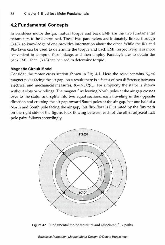
4.2 Fundamental Concepts

In brushless motor design, mutual torque and back EMF are the two fundamental parameters to be determined. These two parameters are intimately linked through (3.43), so knowledge of one provides information about the other. While the BLi and BLv laws can be used to determine the torque and back EMF respectively, it is more convenient to compute flux linkage, and then employ Faraday's law to obtain the back EMF. Then, (3.43) can be used to determine torque.

Magnetic Circuit Model Consider the motor cross section shown in Fig. 4-1. Here the rotor contains N,„=4 magnet poles facing the air gap. As a result there is a factor of two difference between electrical and mechanical measures, 6e=(Nm/2)6m. For simplicity the stator is shown without slots or windings. The magnet flux leaving North poles at the air gap crosses over to the stator and splits into two equal sections, each traveling in the opposite direction and crossing the air gap toward South poles at the air gap. For one half of a North and South pole facing the air gap, this flux flow is illustrated by the flux path on the right side of the figure. Flux flowing between each of the other adjacent half pole pairs follows accordingly.

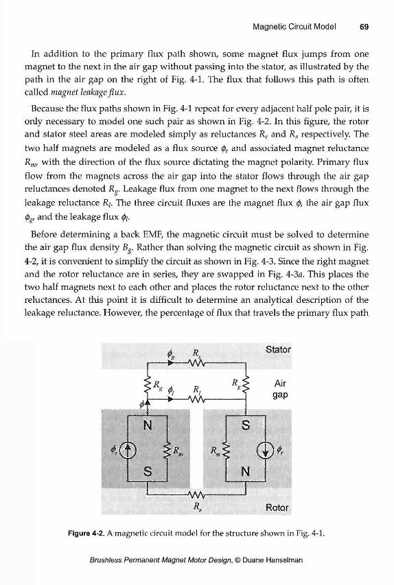
In addition to the primary flux path shown, some magnet flux jumps from one magnet to the next in the air gap without passing into the stator, as illustrated by the path in the air gap on the right of Fig. 4-1. The flux that follows this path is often called magnet leakage flux.

Because the flux paths shown in Fig. 4-1 repeat for every adjacent half pole pair, it is only necessary to model one such pair as shown in Fig. 4-2. In this figure, the rotor and stator steel areas are modeled simply as reluctances Rr and Rs respectively. The two half magnets are modeled as a flux source tpr and associated magnet reluctance Rm, with the direction of the flux source dictating the magnet polarity. Primary flux flow from the magnets across the air gap into the stator flows through the air gap reluctances denoted Rg. Leakage flux from one magnet to the next flows through the leakage reluctance R/. The three circuit fluxes are the magnet flux 0, the air gap flux <(>g, and the leakage flux fy.

Before determining a back EMF, the magnetic circuit must be solved to determine the air gap flux density Bg. Rather than solving the magnetic circuit as shown in Fig. 4-2, it is convenient to simplify the circuit as shown in Fig. 4-3. Since the right magnet and the rotor reluctance are in series, they are swapped in Fig. 4-3c. This places the two half magnets next to each other and places the rotor reluctance next to the other reluctances. At this point it is difficult to determine an analytical description of the leakage reluctance. However, the percentage of flux that travels the primary flux path

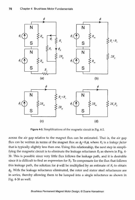
(a) (b)

(o)

2 K A

(d)

Figure 4-3. Simplifications of the magnetic circuit in Fig. 4-2.

across the air gap relative to the magnet flux can be estimated. That is, the air gap flux can be written in terms of the magnet flux as (ps=Ki<p, where K/ is a leakage factor that is typically slightly less than one. Using this relationship, the next step in simpli-fying the magnetic circuit is to eliminate the leakage reluctance Ri as shown in Fig. 4-3b. This is possible since very little flux follows the leakage path, and it is desirable since it is difficult to find an expression for R/. To compensate for the flux that follows this leakage path, the solution for 0 will be multiplied by an estimate of K/ to obtain (pg. With the leakage reluctance eliminated, the rotor and stator steel reluctances are in series, thereby allowing them to be lumped into a single reluctance as shown in Fig. 4-3b as well.

The two magnet halves in series in Fig. 4-3b can be simplified as shown in Fig. 4-3c. From an electrical circuit point of view, the simplified magnet shown in Fig. 4-3c is found by determining the Norton equivalent circuit of the two series magnet halves. That is, the simplified flux source is (pr since that is the flux that would flow if a "short" were placed across the series magnets, and 2Rm is the equivalent reluctance seen looking into the circuit formed by the two series magnets. From a magnetic material point of view, the two half magnets in series is equivalent to a single block of permanent magnet material having twice the length. Therefore, (¡)r remains unchanged but R,n doubles since reluctance is directly proportional to material length.

The steel reluctance Rr+Rs in Fig. 4-3c is nonlinear because of the saturation charac-teristic of ferromagnetic materials. Therefore, this reluctance must be eliminated in some way to find an analytic solution. As long as the permeability of the steel is high relative to air, the steel reluctance will be small relative to the air gap reluctance Rg as demonstrated in the example in Chapter 2. When this is true, the steel reluctance can be thought of as a perturbation of the air gap reluctance. That is, the steel reluctance can be eliminated by introducing a reluctance factor Kr as shown in Fig. 4-3d. Here Kr

is a constant slightly greater than one that increases the air gap reluctance slightly to accommodate or compensate for the missing steel reluctance.

It is important to note that in practice one seldom tries to determine analytical expressions for the leakage factor K/ and reluctance factor Kr. It is simply too difficult to determine accurate values given the simple modeling being performed here. Their values are usually chosen based on the experience of the designer.

Magnetic Circuit Solution Given the magnetic circuit in Fig. 4-3d, the magnet flux 0 can be expressed using flux division as (i.e., as in current division between resistors in an electrical circuit)

Based on and general expressions for the magnet and air gap reluctances, i.e.,

2 Rm

2 Rm +2 KrRg •m (4.1)

R =—— ni ,

iuRPo/im

8 (4.2)

the air gap flux can be written as

(4.3)

where lm and Am are the magnet length and cross-sectional area respectively, and g and Ag are the air gap length and cross-sectional area respectively. Substituting the flux concentration factor C<p=Am/Ag from (2.30), the flux density relationships Bs=(j)g/Ag

and Br=(pr/Amr and the permeance coefficient from (2.33) as Pc=/m/(gQ) i n t o ( 4 - 3 ) gives an air gap flux density of

This equation describes the air gap flux density crossing the air gap. For the motor being considered here with surface magnets, the leakage factor is typically in the range 0.9<K/<1.0, the reluctance factor is in the range 1.0<Kr<1.2, and the flux con-centration factor is ideally 1.0. If one considers these values to be fixed and the rema-nence Br to be fixed by the magnet choice, the permeance coefficient Pc determines the amplitude of the air gap flux density. As the permeance coefficient increases, the air gap flux density approaches a maximum that is slightly less than the remanence. Without flux concentration, it is not possible to achieve an air gap flux density Bg

greater than Br Moreover, the relationship between permeance coefficient and air gap flux density is nonlinear. The air gap flux density approaches the remanence asymptotically. Doubling Pc does not double However, doubling Pc means dou-bling the magnet length, which doubles its volume and associated cost. For typical parameter values, Fig. 4-4 demonstrates the relationship between permeance coeffi-cient and the ratio Bg/Br, where the vertical lines mark the typical four to six per-meance coefficient range used in many motor designs.

The flux density in (4.4) defines an approximation to the air gap flux density over the surface of the magnet pole. That is, (4.4) gives the amplitude of the air gap flux density IB I as shown in Fig. 4-5. Over North poles, (4.4) gives the positive ampli-tude, and over South poles, (4,4) gives the negative amplitude. While this approxima-tion is far from exact, the derivation of (4.4) provides valuable insight into motor operation, and (4.4) itself illustrates fundamental principles that exist even when more accurate modeling is performed.

B (4.4)

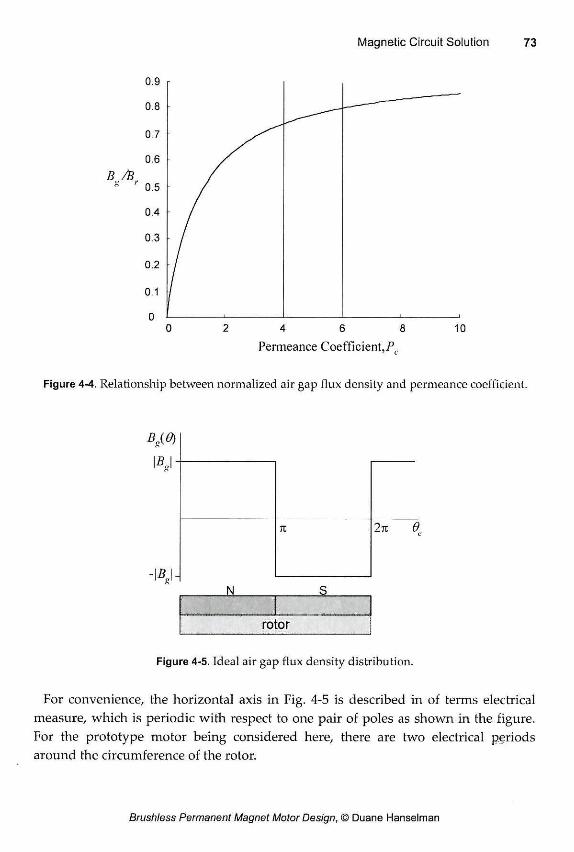
Permeance Coefficient,Pc

Figure 4-4. Relationship between normalized air gap flux density and permeance coefficient.

Figure 4-5. Ideal air gap flux density distribution.

For convenience, the horizontal axis in Fig. 4-5 is described in of terms electrical measure, which is periodic with respect to one pair of poles as shown in the figure. For the prototype motor being considered here, there are two electrical periods around the circumference of the rotor.

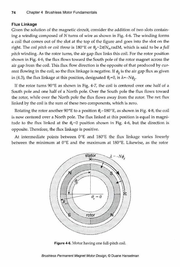
Flux Linkage Given the solution of the magnetic circuit, consider the addition of two slots contain-ing a winding composed of N turns of wire as shown in Fig. 4-6. The winding forms a coil that comes out of the slot at the top of the figure and goes into the slot on the right. The coil pitch or coil throw is 180°E or 0p=27t/NmradM, which is said to be a full pitch winding. As the rotor turns, the air gap flux links this coil. For the rotor position shown in Fig. 4-6, the flux flows toward the South pole of the rotor magnet across the air gap from the coil. This flux flow direction is the opposite of that produced by cur-rent flowing in the coil, so the flux linkage is negative. If (j)g is the air gap flux as given in (4.3), the flux linkage at this position, designated 0e=0, is A=-N0?.

If the rotor turns 90°E as shown in Fig. 4-7, the coil is centered over one half of a South pole and one half of a North pole. Over the South pole the flux flows toward the rotor, while over the North pole the flux flows away from the rotor. The net flux linked by the coil is the sum of these two components, which is zero.

Rotating the rotor another 90 °E to a position 0t,=18O°E, as shown in Fig. 4-8, the coil is now centered over a North pole. The flux linked at this position is equal in magni-tude to the flux linked at the Qe=0 position shown in Fig. 4-6, but the direction is opposite. Therefore, the flux linkage is positive.

At intermediate points between 0°E and 180°E the flux linkage varies linearly between the minimum at 0°E and the maximum at 180°E. Likewise, as the rotor

Figure 4-6. Motor having one full-pitch coil.

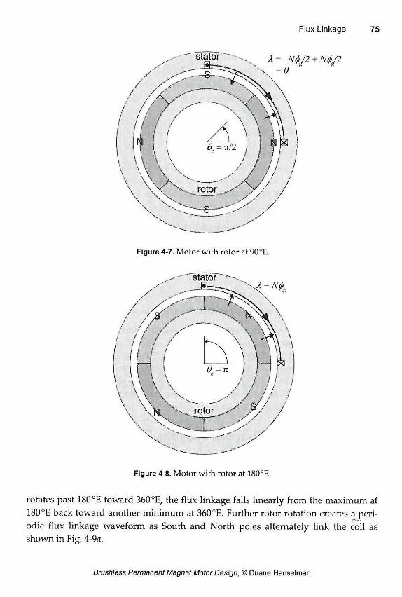
Figure 4-7. Motor with rotor at 90°E.

rotates past 180°E toward 360°E, the flux linkage falls linearly from the maximum at 180°E back toward another minimum at 360°E. Further rotor rotation creates a peri-odic flux linkage waveform as South and North poles alternately link the coil as shown in Fig. 4-9a.

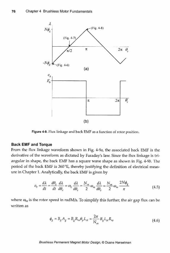
(a)

71 2 TT

(b)

Figure 4-9. Flux linkage and back EMF as a function of rotor position.

Back EMF and Torque From the flux linkage waveform shown in Fig. 4-9a, the associated back EMF is the derivative of the waveform as dictated by Faraday's law. Since the flux linkage is tri-angular in shape, the back EMF has a square wave shape as shown in Fig. 4-9b. The period of the back EMF is 360 °E, thereby justifying the definition of electrical meas-ure in Chapter 1. Analytically, the back EMF is given by

dX dde dX dX N d X Nm 2Ntf> eb = — = —i = co, = —^co... = ——a>„. - .. (-\

! dt dt d0c L d6e 2 dQe 2 7i (4'5>

where com is the rotor speed in radM/s. To simplify this further, the air gap flux can be written as

2 jt = B s A g = BSRroep Lsl = LstRw ( 4 . 6 )

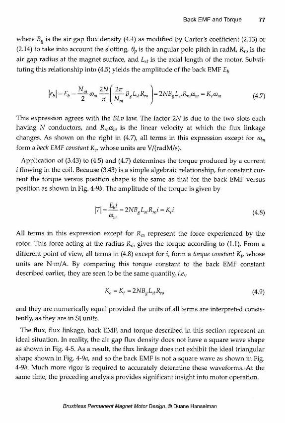
where Bg is the air gap flux density (4.4) as modified by Carter's coefficient (2.13) or (2.14) to take into account the slotting, 6p is the angular pole pitch in radM, Rr0 is the air gap radius at the magnet surface, and Lst is the axial length of the motor. Substi-tuting this relationship into (4.5) yields the amplitude of the back EMF

I I r Nm 2 N ' I K

This expression agrees with the BLv law. The factor 2N is due to the two slots each having N conductors, and Rrocon, is the linear velocity at which the flux linkage changes. As shown on the right in (4.7), all terms in this expression except for com

form a back EMF constant Ke, whose units are V/(radM/s).

Application of (3.43) to (4.5) and (4.7) determines the torque produced by a current i flowing in the coil. Because (3.43) is a simple algebraic relationship, for constant cur-rent the torque versus position shape is the same as that for the back EMF versus position as shown in Fig. 4-%. The amplitude of the torque is given by

\T\ = 5± = 2NBgLstRroi = Kti ( 4 8 )

All terms in this expression except for Rro represent the force experienced by the rotor. This force acting at the radius Rro gives the torque according to (1.1). From a different point of view, all terms in (4.8) except for i, form a torque constant Kt, whose units are N-m/A. By comparing this torque constant to the back EMF constant described earlier, they are seen to be the same quantity, i.e.,

Ke=Kt=2NBgLstRro (4.9)

and they are numerically equal provided the units of all terms are interpreted consis-tently, as they are in SI units.

The flux, flux linkage, back EMF, and torque described in this section represent an ideal situation. In reality, the air gap flux density does not have a square wave shape as shown in Fig. 4-5. As a result, the flux linkage does not exhibit the ideal triangular shape shown in Fig. 4-9fl, and so the back EMF is not a square wave as shown in Fig. 4-9b. Much more rigor is required to accurately determine these waveforms.-At the same time, the preceding analysis provides significant insight into motor operation.

2 TV N,„

BgLstRro = 2 NBgLstRrocûm=Keù)„ (4.7)

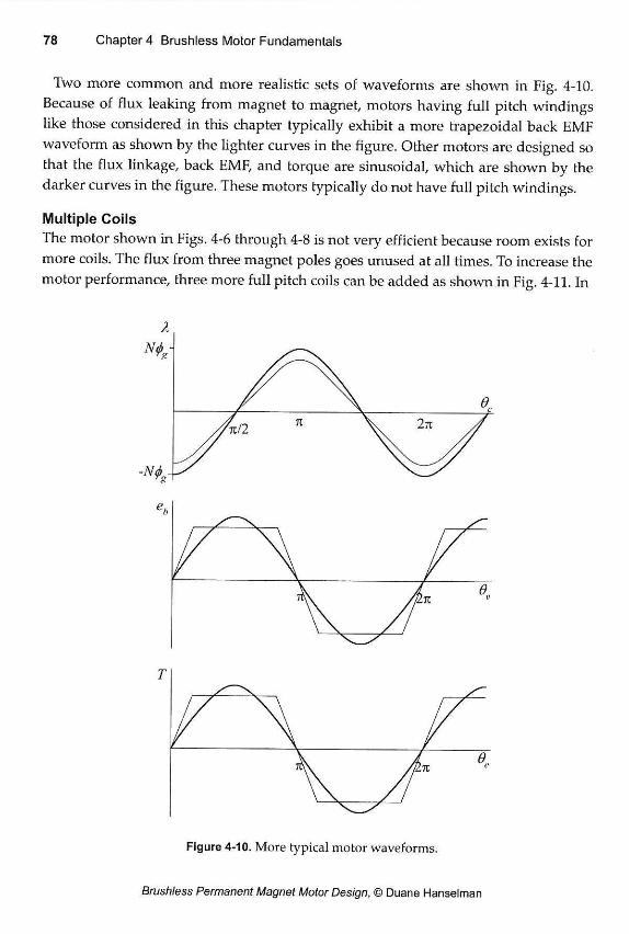
Two more common and more realistic sets of waveforms are shown in Fig. 4-10. Because of flux leaking from magnet to magnet, motors having full pitch windings like those considered in this chapter typically exhibit a more trapezoidal back EMF waveform as shown by the lighter curves in the figure. Other motors are designed so that the flux linkage, back EMF, and torque are sinusoidal, which are shown by the darker curves in the figure. These motors typically do not have full pitch windings.

Multiple Coils The motor shown in Figs. 4-6 through 4-8 is not very efficient because room exists for more coils. The flux from three magnet poles goes unused at all times. To increase the motor performance, three more full pitch coils can be added as shown in Fig. 4-11. In

Figure 4-10. More typical motor waveforms.

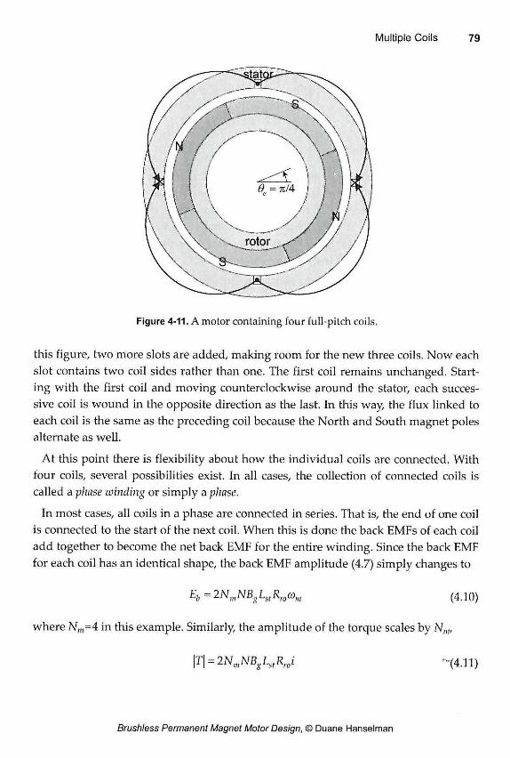
Figure 4-11. A motor containing four full-pitch coils.

this figure, two more slots are added, making room for the new three coils. Now each slot contains two coil sides rather than one. The first coil remains unchanged. Start-ing with the first coil and moving counterclockwise around the stator, each succes-sive coil is wound in the opposite direction as the last. In this way, the flux linked to each coil is the same as the preceding coil because the North and South magnet poles alternate as well.

At this point there is flexibility about how the individual coils are connected. With four coils, several possibilities exist. In all cases, the collection of connected coils is called a phase winding or simply a phase.

In most cases, all coils in a phase are connected in series. That is, the end of one coil is connected to the start of the next coil. When this is done the back EMFs of each coil add together to become the net back EMF for the entire winding. Since the back EMF for each coil has an identical shape, the back EMF amplitude (4.7) simply changes to

Eb = 2 Nm NBg Lst Rwco„, (4.10)

where Nm=4 in this example. Similarly, the amplitude of the torque scales by Nm,

\T\ = 2NmNBgLitRJ -(4.11)

This expression confirms that T=kD2L as given by (1.8). One diameter D appears as the radius Rw; the other is implied by the number of magnet poles N„„ and L appears directly as Lst.

4.3 Multiple Phases

The motor considered in the preceding section and shown in Fig. 4-11 is a single phase motor. This motor type does not appear in many applications because it is not possible to produce torque at all rotor positions. Once every 180°E the back EMF and torque cross through zero. At these points, the motor cannot produce torque. Moreo-ver, if the motor comes to rest at these points, the motor cannot be started without physically rotating the shaft to a nonzero torque point.

To eliminate this problem and to make it easier to produce constant torque, brush-less permanent magnet motors contain more than one phase winding, with the indi-vidual phase windings oriented so that their zero crossing points in the back EMF and torque are uniformly distributed over an electrical period. Most brushless per-manent magnet motors have three phases, and some have either one or two phases. Because the number of power electronics devices needed to drive a motor increases with the number of phases, it is very uncommon to see a motor having more than three phases. Only at very high power levels where multiple banks of power elec-tronic devices are required does it make sense to use more than three phases.

The motor shown in Fig. 4-11 can accommodate two additional phase windings, each composed of four coils in the same way that the first phase winding has four coils. The resulting three phase motor is shown in Fig. 4-12, where A, B, and C desig-nate the phases. To avoid making the figure visually confusing, Fig. 4-12 shows only one coil for each phase. The rest are identified by the phase labels near each slot.

The phase A winding shown in Fig. 4-12 matches the phase winding described ear-lier in Fig. 4-11. Since there are three phases, the zero crossings of the back EMF and torque are separated by (360°E)/3, which is 120°E or 60°M. Therefore the slots for phase B are rotated 60°M from the corresponding slots of phase A, and the slots of phase C are rotated 60°M from the corresponding slots of phase B. This arrangement places slots around the circumference of the stator every 30°M as shown in the fig-ure. The resulting phase waveforms are shown in Fig. 4-13. Since the rotor is unchanged, the flux linkage, back EMF, and torque of phase B will have the same shape as corresponding phase A waveforms, but will be delayed by the 120°E offset due to the 120 °E offset in slot placement. Likewise phase C waveforms look like phase A waveforms displaced by 240 °E.

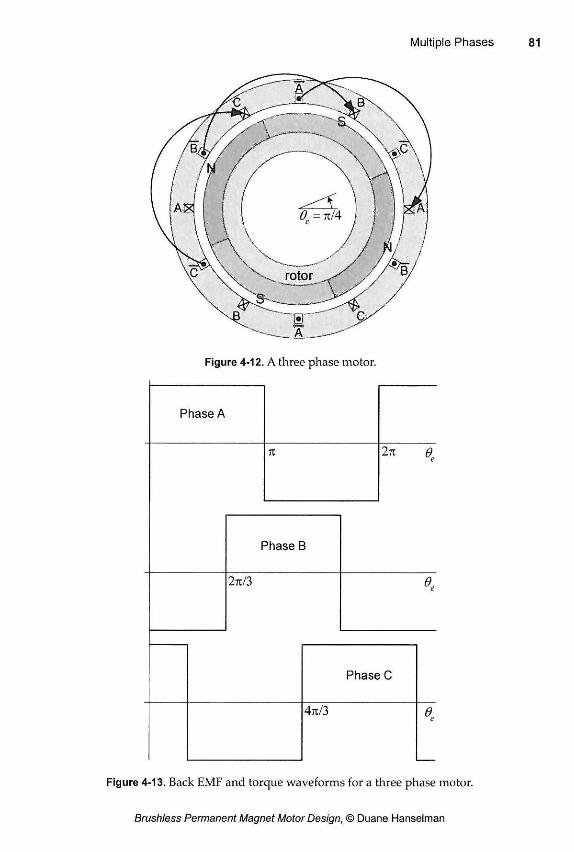
Figure 4-12. A three phase motor.

Phase A

Phase B

2tt/3

Phase C

4n/3

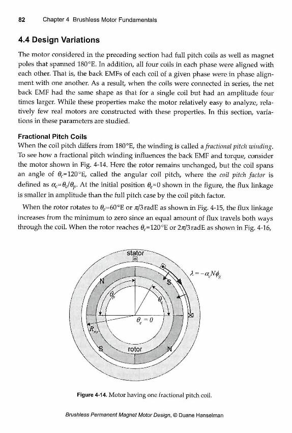
4.4 Design Variations

The motor considered in the preceding section had full pitch coils as well as magnet poles that spanned 180°E. In addition, all four coils in each phase were aligned with each other. That is, the back EMFs of each coil of a given phase were in phase align-ment with one another. As a result, when the coils were connected in series, the net back EMF had the same shape as that for a single coil but had an amplitude four times larger. While these properties make the motor relatively easy to analyze, rela-tively few real motors are constructed with these properties. In this section, varia-tions in these parameters are studied.

Fractional Pitch Coils When the coil pitch differs from 180°E, the winding is called a fractional pitch winding. To see how a fractional pitch winding influences the back EMF and torque, consider the motor shown in Fig. 4-14. Here the rotor remains unchanged, but the coil spans an angle of 0C= 120°E, called the angular coil pitch, where the coil pitch factor is defined as ac=6c/6p. At the initial position 0e=O shown in the figure, the flux linkage is smaller in amplitude than the full pitch case by the coil pitch factor.

When the rotor rotates to 0e=60°E or ;r/3radE as shown in Fig. 4-15, the flux linkage increases from the minimum to zero since an equal amount of flux travels both ways through the coil. When the rotor reaches 0C.=12O°E or 2^/3radE as shown in Fig. 4-16,

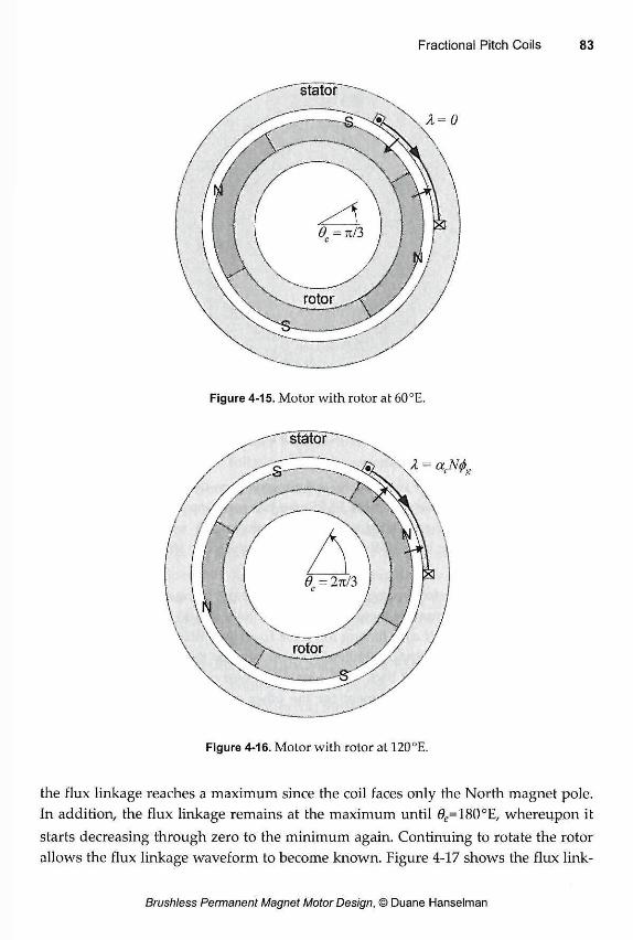
Figure 4-15. Motor with rotor at 60°E.

Figure 4-16. Motor with rotor at 120°E.

the flux linkage reaches a maximum since the coil faces only the North magnet pole. In addition, the flux linkage remains at the maximum until 0C=18O°E, whereupon it starts decreasing through zero to the minimum again. Continuing to rotate the rotor allows the flux linkage waveform to become known. Figure 4-17 shows the flux link-

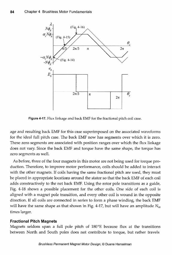
Figure 4-17. Flux linkage and back EMF for the fractional pitch coil case.

age and resulting back EMF for this case superimposed on the associated waveforms for the ideal full pitch case. The back EMF now has segments over which it is zero. These zero segments are associated with position ranges over which the flux linkage does not vary. Since the back EMF and torque have the same shape, the torque has zero segments as well.

As before, three of the four magnets in this motor are not being used for torque pro-duction. Therefore, to improve motor performance, coils should be added to interact with the other magnets. If coils having the same fractional pitch are used, they must be placed in appropriate locations around the stator so that the back EMF of each coil adds constructively to the net back EMF. Using the rotor pole transitions as a guide, Fig. 4-18 shows a possible placement for the other coils. One side of each coil is aligned with a magnet pole transition, and every other coil is wound in the opposite direction. If all coils are connected in series to form a phase winding, the back EMF will have the same shape as that shown in Fig. 4-17, but will have an amplitude Nm

times larger.

Fractional Pitch Magnets Magnets seldom span a full pole pitch of 180°E because flux at the transitions between North and South poles does not contribute to torque, but rather travels

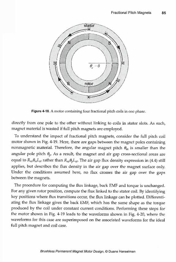
Figure 4-18. A motor containing four fractional pitch coils in one phase.

directly from one pole to the other without linking to coils in stator slots. As such, magnet material is wasted if full pitch magnets are employed.

To understand the impact of fractional pitch magnets, consider the full pitch coil motor shown in Fig. 4-19. Here, there are gaps between the magnet poles containing nonmagnetic material. Therefore, the angular magnet pitch 6 m is smaller than the angular pole pitch 6p. As a result, the magnet and air gap cross-sectional areas are equal to RroOmLst rather than Rr0GpLst. The air gap flux density expression in (4.4) still applies, but describes the flux density in the air gap over the magnet surface only. Under the conditions assumed here, no flux crosses the air gap over the gaps between the magnets.

The procedure for computing the flux linkage, back EMF and torque is unchanged. For any given rotor position, compute the flux linked to the stator coil. By identifying key positions where flux transitions occur, the flux linkage can be plotted. Differenti-ating the flux linkage gives the back EMF, which has the same shape as the torque produced by the coil under constant current conditions. Performing these steps for the motor shown in Fig. 4-19 leads to the waveforms shown in Fig. 4-20, where the waveforms for this case are superimposed on the associated waveforms for the ideal full pitch magnet and coil case.

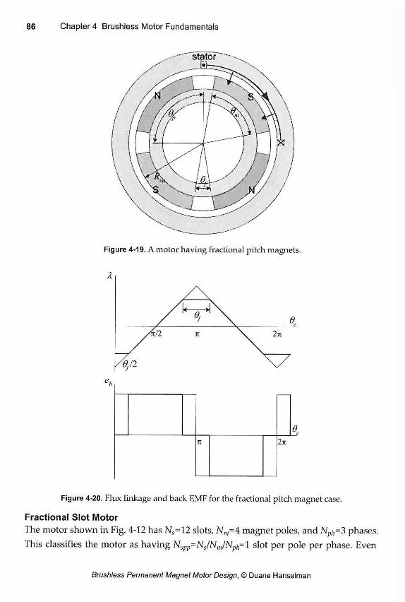
Figure 4-19. A motor having fractional pitch magnets.

Figure 4-20. Flux linkage and back EMF for the fractional pitch magnet case.

Fractional Slot Motor

The motor shown in Fig. 4-12 has Ns= 12 slots, Nm=4 magnet poles, and Nph=3 phases. This classifies the motor as having Nm,=Ns/Nin/Nph=l slot per pole per phase. Even

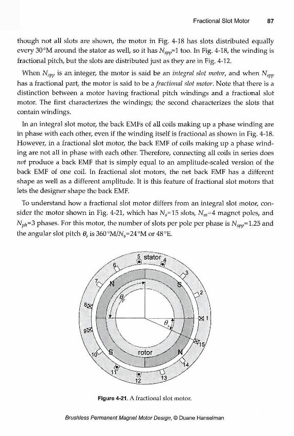
though not all slots are shown, the motor in Fig. 4-18 has slots distributed equally every 30°M around the stator as well, so it has Nspp= 1 too. In Fig. 4-18, the winding is fractional pitch, but the slots are distributed just as they are in Fig. 4-12.

When Nspp is an integer, the motor is said be an integral slot motor, and when Nspp has a fractional part, the motor is said to be a fractional slot motor. Note that there is a distinction between a motor having fractional pitch windings and a fractional slot motor. The first characterizes the windings; the second characterizes the slots that contain windings.

In an integral slot motor, the back EMFs of all coils making up a phase winding are in phase with each other, even if the winding itself is fractional as shown in Fig. 4-18. However, in a fractional slot motor, the back EMF of coils making up a phase wind-ing are not all in phase with each other. Therefore, connecting all coils in series does not produce a back EMF that is simply equal to an amplitude-scaled version of the back EMF of one coil. In fractional slot motors, the net back EMF has a different shape as well as a different amplitude. It is this feature of fractional slot motors that lets the designer shape the back EMF.

To understand how a fractional slot motor differs from an integral slot motor, con-sider the motor shown in Fig. 4-21, which has Ns= 15 slots, N,„=4 magnet poles, and Nph=3 phases. For this motor, the number of slots per pole per phase is Nspp= 1.25 and the angular slot pitch ds is 360°M/NS=24°M or 48°E.

Figure 4-21. A fractional slot motor.

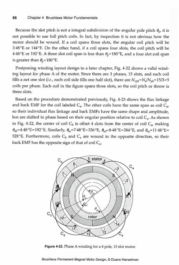
Because the slot pitch is not a integral subdivision of the angular pole pitch 6p, it is not possible to use full pitch coils. In fact, by inspection it is not obvious how the motor should be wound. If a coil spans three slots, the angular coil pitch will be 3-48 °E or 144°E. On the other hand, if a coil spans four slots, the coil pitch will be 4-48 °E or 192°E. A three slot coil span is less than 6>/(=180oE, and a four slot coil span is greater than 0/;=18O°E.

Postponing winding layout design to a later chapter, Fig. 4-22 shows a valid wind-ing layout for phase A of the motor. Since there are 3 phases, 15 slots, and each coil fills a net one slot (i.e., each coil side fills one half slot), there are Ncph=NJNph= 15/3=5 coils per phase. Each coil in the figure spans three slots, so the coil pitch or throw is three slots.

Based on the procedure demonstrated previously, Fig. 4-23 shows the flux linkage and back EMF for the coil labeled Ca . The other coils have the same span as coil Q, so their individual flux linkage and back EMFs have the same shape and amplitude, but are shifted in phase based on their angular position relative to coil Ca. As shown in Fig. 4-22, the center of coil Q, is offset 4 slots from the center of coil Ca, making 0^=4-48 °E=192 °E. Similarly, 0£J(-=7-48oE=336°E, 0(irf=8-48°E=384°E/ and 0„e=1148°E= 528°E. Furthermore, coils Cb and Ce are wound in the opposite direction, so their back EMF has the opposite sign of that of coil Ca.

Figure 4-22. Phase A winding for a 4 pole, 15 slot motor.

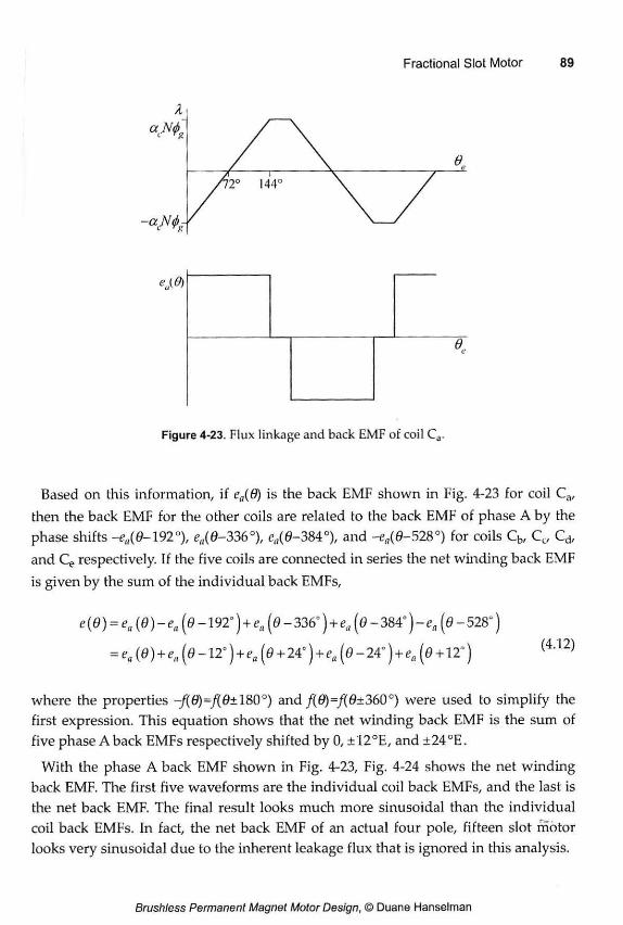
0.

Figure 4-23. Flux linkage and back EMF of coil C a .

Based on this information, if ea(0) is the back EMF shown in Fig. 4-23 for coil Ca, then the back EMF for the other coils are related to the back EMF of phase A by the phase shifts -ea(d-l92°), ea(0-336°), e„(0-384°), and -en(d-528°) for coils Cb, Cc/ Cd, and Ce respectively. If the five coils are connected in series the net winding back EMF is given by the sum of the individual back EMFs,

e(O) = ea{0)-ea(O-l9T) + ea(O-336°) + ea(6-384°)~ea (6-528")

= ea(d) + ea(G-lT) + ea(e + 24°) + ea(d-24°) + ea(d + ir) ( 4 ' 1 2 )

where the properties -/(0)=/(0±18O°) and f(6)=f(d±360°) were used to simplify the first expression. This equation shows that the net winding back EMF is the sum of five phase A back EMFs respectively shifted by 0, ±12°E, and ±24°E.

With the phase A back EMF shown in Fig. 4-23, Fig. 4-24 shows the net winding back EMF. The first five waveforms are the individual coil back EMFs, and the last is the net back EMF. The final result looks much more sinusoidal than the individual coil back EMFs. In fact, the net back EMF of an actual four pole, fifteen slot motor looks very sinusoidal due to the inherent leakage flux that is ignored in this analysis.

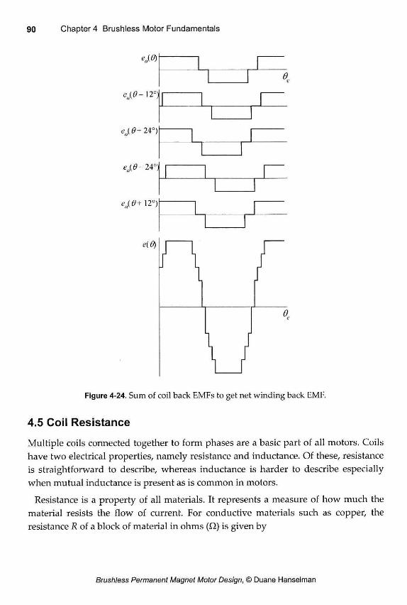
ea{0- 12°)

e(0+ 24°)

e„(0-24c

12°)

Figure 4-24. Sum of coil back EMFs to get net winding back EMF.

4.5 Coil Resistance

Multiple coils connected together to form phases are a basic part of all motors. Coils have two electrical properties, namely resistance and inductance. Of these, resistance is straightforward to describe, whereas inductance is harder to describe especially when mutual inductance is present as is common in motors.

Resistance is a property of all materials. It represents a measure of how much the material resists the flow of current. For conductive materials such as copper, the resistance R of a block of material in ohms (Q) is given by

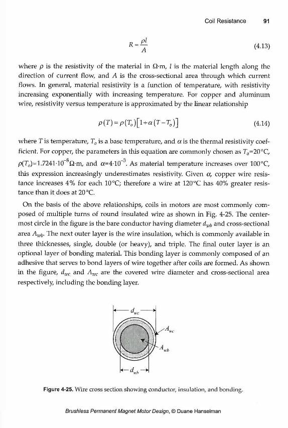
where p is the resistivity of the material in £2-m, I is the material length along the direction of current flow, and A is the cross-sectional area through which current flows. In general, material resistivity is a function of temperature, with resistivity increasing exponentially with increasing temperature. For copper and aluminum wire, resistivity versus temperature is approximated by the linear relationship

p(T) = p(T0)[l + a(T-T0)] (4.14)

where Tis temperature, T0 is a base temperature, and a is the thermal resistivity coef-ficient. For copper, the parameters in this equation are commonly chosen as T0=20°C,

—8 —3 p(T0)=1.7241 -10 Q-m, and a=4-10 . As material temperature increases over 100°C, this expression increasingly underestimates resistivity. Given a, copper wire resis-tance increases 4% for each 10°C; therefore a wire at 120 °C has 40% greater resis-tance than it does at 20 °C.

On the basis of the above relationships, coils in motors are most commonly com-posed of multiple turns of round insulated wire as shown in Fig. 4-25. The center-most circle in the figure is the bare conductor having diameter dwi} and cross-sectional area Awb, The next outer layer is the wire insulation, which is commonly available in three thicknesses, single, double (or heavy), and triple. The final outer layer is an optional layer of bonding material. This bonding layer is commonly composed of an adhesive that serves to bond layers of wire together after coils are formed. As shown in the figure, dwc and Awc are the covered wire diameter and cross-sectional area respectively, including the bonding layer.

Several standards exist for classifying wire according to diameter. One common standard is American Wire Gage (AWG). In AWG, standard wire diameters form a geometric progression described by the relationship

dwb = 8.251463(0.8905257)° (4.15)

where G is the integer wire gage, and dwb is the bare wire diameter in mm. There is an inverse relationship between wire gage and diameter. As the gage increases, the diameter decreases. Alternatively, as the gage increases, the resistance per unit length increases. The inverse of the above relationship is

* ( 8.251463 ] (4.16) log (0.8905257)

Because AWG is based on a geometric progression, wire gages are related to each other by ratios as shown in Fig. 4-26. This figure plots resistance relative to a wire having any gage G to wires having gages G, G+l, etc. The most notable point on the curve appears at G+3. A wire of gage G+3 has twice the resistance of a wire of gage G. So two wires of gage G+3 taken in parallel have the same resistance as one wire of gage G. Other important points appear at G-l and G+l. At G+l, resistance is approxi-mately 26% greater than that at G. So increasing the wire gage by one, increases resis-tance and I2R losses by 26% provided current remains constant. Alternatively, at G-l, resistance decreases approximately to about 79% of that at G. Therefore, decreasing the wire gage by one, decreases the I2R losses for fixed current to 79% of what they are at G.

The current capacity of the wire depends on its cross-sectional area and its thermal environment. The heat density in a resistance, i.e., I2R loss per unit volume, is equal

to p/2, where J is the current density in the material. Based on experience, the maxi-2

mum allowable current density varies roughly between 1 and 10Arms/mm . Using these limits as a guideline, Fig. 4-27 shows the allowable RMS wire current versus wire gage. In confined volumes with little thermal conductivity, the lower limit of 1 Arms/mm2 may be too high. Similarly, if wire is actively cooled, 10 Arms/mm" may be overly conservative as an upper limit. It is interesting to note that the rated current for 14 gage household wiring is 15 Arms, which corresponds to a current density of

2 7.2 Arms/mm".

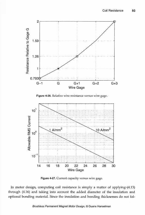
G-1 G G+1 G+2 G+3 Wire Gage

Figure 4-26. Relative wire resistance versus wire gage.

1 0 '

c Q) i—

o C0 è 10L

JD -Q CO §

o

10 - 1

14 16 18 20 22 24 26 28 30 Wire Gage

Figure 4-27. Current capacity versus wire gage.

In motor design, computing coil resistance is simply a matter of applying (4.13) through (4.16) and taking into account the added diameter of the insulation and optional bonding material. Since the insulation and bonding thicknesses do not fol-

low a geometric progression, (4.15) or a similar equation cannot be used to compute the covered diameter dwc. The single, double, and triple insulation thicknesses and the bonding thicknesses do not conform to any smooth function with respect to wire gage, so they are best determined by consulting a manufacturer's wire table.

4.6 Coil Inductance

Inductance is not usually a critical parameter in brushless permanent magnet motors. Inductance determines the time constant of the windings, and therefore, determines the rate at which winding currents can change. Modern power electronic control techniques that rely on current control principles are relatively insensitive to the exact inductance value. As a result, inductance calculations are often simplified to produce analytical inductance estimates. If greater accuracy is required, three-dimensional finite element analysis is required.

When a coil is placed in stator slots, its inductance changes dramatically compared to its inductance when surrounded by air. Computing coil inductance is a matter of determining the magnetic field created by coil current and then relating this field to inductance through the use of (3.4). Alternatively, inductance can be computed by equating the coenergy stored in an inductance (3.26) to the coenergy stored in the field created by the coil (3.27). That is, inductance can be found by solving

for the inductance L, where V is the volume containing the field.

In addition to self inductance as described above, mutual inductance exists between the coils in a given phase as well as between the coils in different phases. Mutual inductance between coils in a given phase is considered here, but mutual inductance between coils in different phases is not. Because mutual inductance between phases is small relative to self inductance (e.g., around 10%) and because mutual inductance requires much more careful computation using these same general procedures, it will not be considered here.

When coils are placed in slots, the coil inductance has three distinct components due to the three distinct areas where significant magnetic field is created by coil cur-rent. These three areas are the air gap, the slots, and the end turns. The ferromagnetic portions of the motor do not contribute to the inductance as long as their relative per-meability is high. Moreover, magnet flux does not contribute to inductance because inductance relates coil current to the flux linkage created by the coil current acting

(4.17)

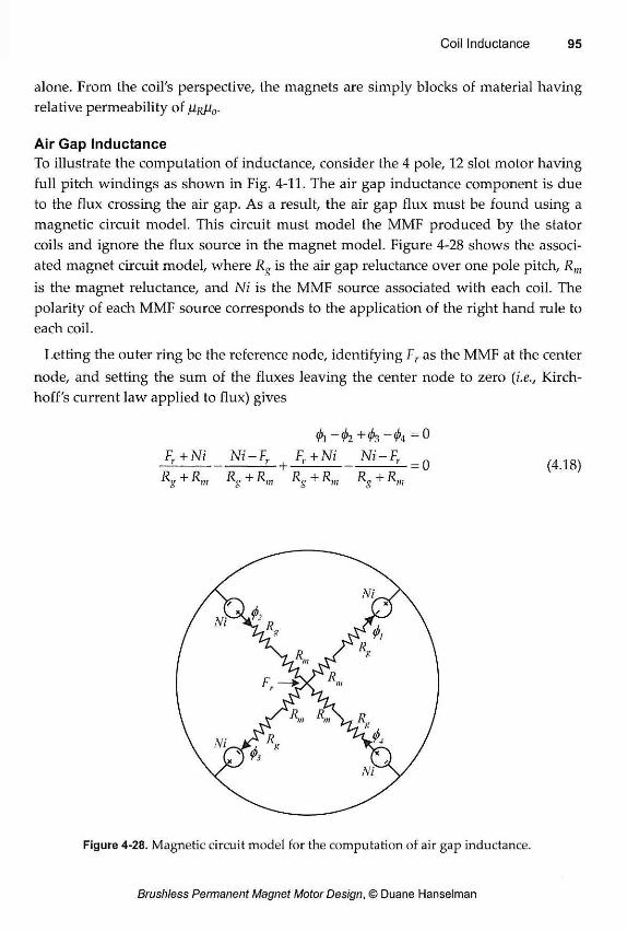
alone. From the coil's perspective, the magnets are simply blocks of material having relative permeability of

Air Gap Inductance To illustrate the computation of inductance, consider the 4 pole, 12 slot motor having full pitch windings as shown in Fig. 4-11. The air gap inductance component is due to the flux crossing the air gap. As a result, the air gap flux must be found using a magnetic circuit model. This circuit must model the MMF produced by the stator coils and ignore the flux source in the magnet model. Figure 4-28 shows the associ-ated magnet circuit model, where Rg is the air gap reluctance over one pole pitch, Rm

is the magnet reluctance, and Ni is the MMF source associated with each coil. The polarity of each MMF source corresponds to the application of the right hand rule to each coil.

Letting the outer ring be the reference node, identifying Fr as the MMF at the center node, and setting the sum of the fluxes leaving the center node to zero (i.e., Kirch-hoff's current law applied to flux) gives

0! + 0 3 - 0 4 = 0 Fr + Ni Ni - Fr

Rg+Rm Rg+Rm

| Fr + Ni Ni - Fr _Q

Rg+Rm Rg + Rm (4.18)

Figure 4-28. Magnetic circuit model for the computation of air gap inductance.

Simplifying the last expression leads to the result Fr=0, which implies that

(4.19)

Therefore, the net flux linked by all four coils is

(4.20)

where Nm=4 is the number of coils (and magnet poles). Using the definition of induc-tance (3.4), the air gap inductance is

Using expressions for the magnet and air gap reluctances (4.2) and the air gap cross-sectional area Ag= Lst6pRro=(27z/Nm)LstRro, where Lst is the axial motor length and Rro

is the air gap radius as shown in Fig. 4-6, yields

where N is the number of turns per coil. This air gap inductance assumes that all four coils are connected in series and is therefore the air gap inductance of the complete phase winding. This expression applies to all full pitch winding cases since Nm does not appear in (4.22). In addition, the air gap inductance is proportional to the rotor surface area, since 2nRroLsl appears in the numerator. The denominator is the mag-netic length from the stator surface through the air gap and magnet to the rotor yoke.

Modifications to the above equation are required when the individual coils are con-nected in parallel or in some combination of series and parallel. These modifications are covered later in this chapter.

Slot Leakage Inductance In addition to the air gap, coil current produces a magnetic field that crosses from one side of a slot to the other as shown in Fig. 4-29. This field makes sense when one considers that a magnetic field circulates around conductors, which in this case are

I - * =

8 i V R < " (4.21)

7 _ 2Kl-loLst Rro k j 2 8 I

(4.22)

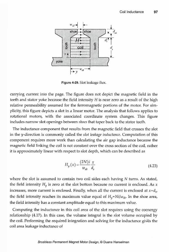
Figure 4-29. Slot leakage flux.

carrying current into the page. The figure does not depict the magnetic field in the teeth and stator yoke because the field intensity H is near zero as a result of the high relative permeability assumed for the ferromagnetic portions of the motor. For sim-plicity, this figure depicts a slot in a linear motor. The analysis that follows applies to rotational motors, with the associated coordinate system changes. This figure includes narrow slot openings between shoes that taper back to the stator teeth.

The inductance component that results from the magnetic field that crosses the slot in the y-direction is commonly called the slot leakage inductance. Computation of this component requires more work than calculating the air gap inductance because the magnetic field linking the coil is not constant over the cross section of the coil, rather it is approximately linear with respect to slot depth, which can be described as

H „ M = (2N)i x

wsb ds (4.23)

where the slot is assumed to contain two coil sides each having N turns. As stated, the field intensity Hy is zero at the slot bottom because no current is enclosed. As x increases, more current is enclosed. Finally, when all the current is enclosed at x-ds, the field intensity reaches its maximum value equal of H^Ni/w^. In the shoe area, the field intensity has a constant amplitude equal to this maximum value.

Computing the inductance in this coil area of the slot requires using the coenergy relationship (4.17). In this case, the volume integral is the slot volume occupied by the coil. Performing the required integration and solving for the inductance gives the coil area leakage inductance of

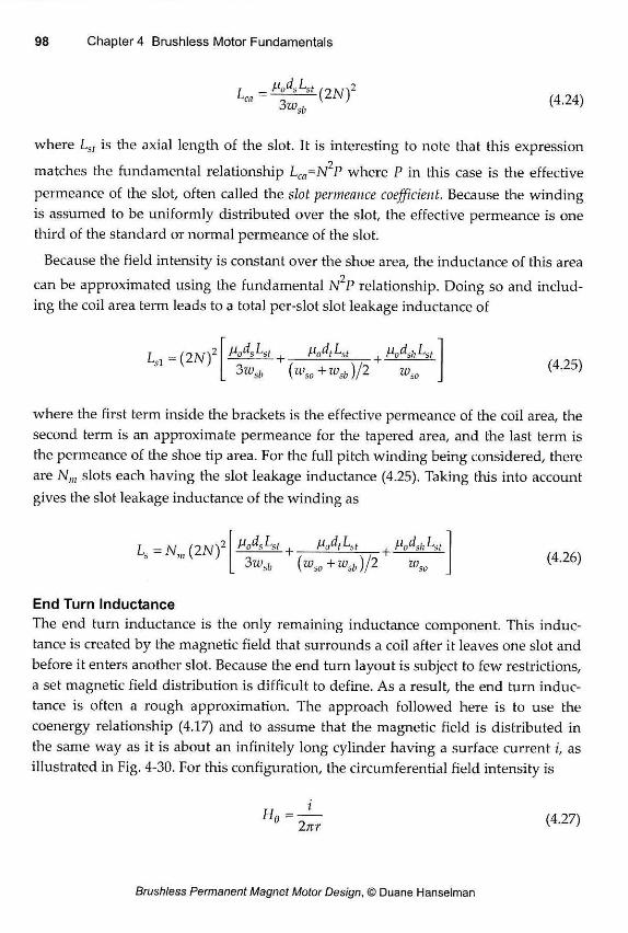
hrn 3 w sb

(4.24)

where Lsi is the axial length of the slot. It is interesting to note that this expression matches the fundamental relationship Lca=N2P where P in this case is the effective permeance of the slot, often called the slot permeance coefficient. Because the winding is assumed to be uniformly distributed over the slot, the effective permeance is one third of the standard or normal permeance of the slot.

Because the field intensity is constant over the shoe area, the inductance of this area can be approximated using the fundamental N P relationship. Doing so and includ-ing the coil area term leads to a total per-slot slot leakage inductance of

=(2 N f PodsLsl H0dtLs

_ 3wsb {wso + wsb )/2 (4.25)

where the first term inside the brackets is the effective permeance of the coil area, the second term is an approximate permeance for the tapered area, and the last term is the permeance of the shoe tip area. For the full pitch winding being considered, there are N„, slots each having the slot leakage inductance (4.25). Taking this into account gives the slot leakage inductance of the winding as

Ls=Nm(2NY PodAt PodtLs Vodsh LSI 3™sb (wso + wsb )/2 VJS

(4.26)

End Turn Inductance The end turn inductance is the only remaining inductance component. This induc-tance is created by the magnetic field that surrounds a coil after it leaves one slot and before it enters another slot. Because the end turn layout is subject to few restrictions, a set magnetic field distribution is difficult to define. As a result, the end turn induc-tance is often a rough approximation. The approach followed here is to use the coenergy relationship (4.17) and to assume that the magnetic field is distributed in the same way as it is about an infinitely long cylinder having a surface current i, as illustrated in Fig. 4-30. For this configuration, the circumferential field intensity is

He = 2 nr (4.27)

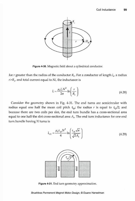
Figure 4-30. Magnetic field about a cylindrical conductor.

for r greater than the radius of the conductor Rc. For a conductor of length le, a radius r>Rc, and total current equal to Ni, the inductance is

Consider the geometry shown in Fig. 4-31. The end turns are semicircular with radius equal one half the mean coil pitch xcp, the radius r is equal to tcp/2; and because there are two coils per slot, the end turn bundle has a cross-sectional area equal to one half the slot cross-sectional area As. The end turn inductance for one end turn bundle having N turns is

L-i—— In — In R..

1

(4.28) " /

Ali Cp . CI) ,,i = L In r —

4 J2AS

WcpN2 , T c p4n \

(4.29) /

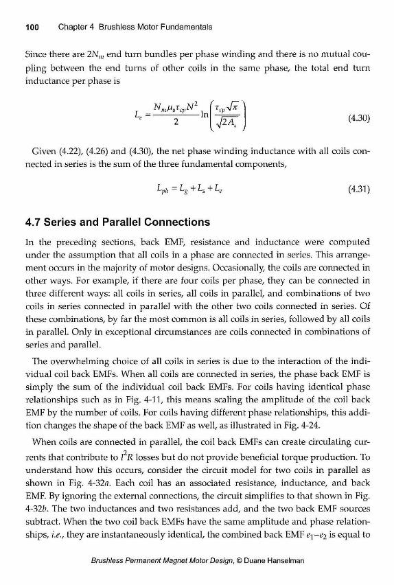
Since there are 2N,„ end turn bundles per phase winding and there is no mutual cou-pling between the end turns of other coils in the same phase, the total end turn inductance per phase is

k> = In JÎÂ; (4.30)

Given (4.22), (4.26) and (4.30), the net phase winding inductance with all coils con-nected in series is the sum of the three fundamental components,

Lpi, - Lg +LS + Le (4.31)

4.7 Series and Parallel Connections

In the preceding sections, back EMF, resistance and inductance were computed under the assumption that all coils in a phase are connected in series. This arrange-ment occurs in the majority of motor designs. Occasionally, the coils are connected in other ways. For example, if there are four coils per phase, they can be connected in three different ways: all coils in series, all coils in parallel, and combinations of two coils in series connected in parallel with the other two coils connected in series. Of these combinations, by far the most common is all coils in series, followed by all coils in parallel. Only in exceptional circumstances are coils connected in combinations of series and parallel.

The overwhelming choice of all coils in series is due to the interaction of the indi-vidual coil back EMFs. When all coils are connected in series, the phase back EMF is simply the sum of the individual coil back EMFs. For coils having identical phase relationships such as in Fig. 4-11, this means scaling the amplitude of the coil back EMF by the number of coils. For coils having different phase relationships, this addi-tion changes the shape of the back EMF as well, as illustrated in Fig. 4-24.

When coils are connected in parallel, the coil back EMFs can create circulating cur-rents that contribute to I R losses but do not provide beneficial torque production. To understand how this occurs, consider the circuit model for two coils in parallel as shown in Fig. 4-32«. Each coil has an associated resistance, inductance, and back EMF. By ignoring the external connections, the circuit simplifies to that shown in Fig. 4-32£>. The two inductances and two resistances add, and the two back EMF sources subtract. When the two coil back EMFs have the same amplitude and phase relation-ships, i.e., they are instantaneously identical, the combined back EMF e\-e2 is equal to

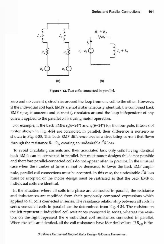
Series and Parallel Connections 101

L

e r e2 Ö

AAA/—

L, + L •2

e e. •2

(a) (b)

Figure 4-32. Two coils connected in parallel.

zero and no current ic circulates around the loop from one coil to the other. However, if the individual coil back EMFs are not instantaneously identical, the combined back EMF e\-e2 is nonzero and current ic circulates around the loop independent of any current applied to the parallel coils during motor operation.

For example, if the back EMFs ea(0-24°) and ea(6+ 24°) for the four pole, fifteen slot motor shown in Fig. 4-24 are connected in parallel, their difference is nonzero as shown in Fig. 4-33. This back EMF difference creates a circulating current that flows through the resistance R1+R2, creating an undesirable I R loss.

To avoid circulating currents and their associated loss, only coils having identical back EMFs can be connected in parallel. For most motor designs this is not possible and therefore parallel-connected coils do not appear often in practice. In the unusual case when the number of turns cannot be decreased to lower the back EMF ampli-tude, parallel coil connections must be accepted. In this case, the undesirable I R loss must be accepted or the motor design must be restricted so that the back EMF of individual coils are identical.

In the situation where all coils in a phase are connected in parallel, the resistance and inductances are modified from their previously computed expressions which applied to all coils connected in series. The resistance relationship between all coils in series versus all coils in parallel can be determined from Fig. 4-34. The resistors on the left represent n individual coil resistances connected in series, whereas the resis-tors on the right represent the n individual coil resistances connected in parallel. When the coils are identical, all the coil resistances have identical values. If Reqs is the

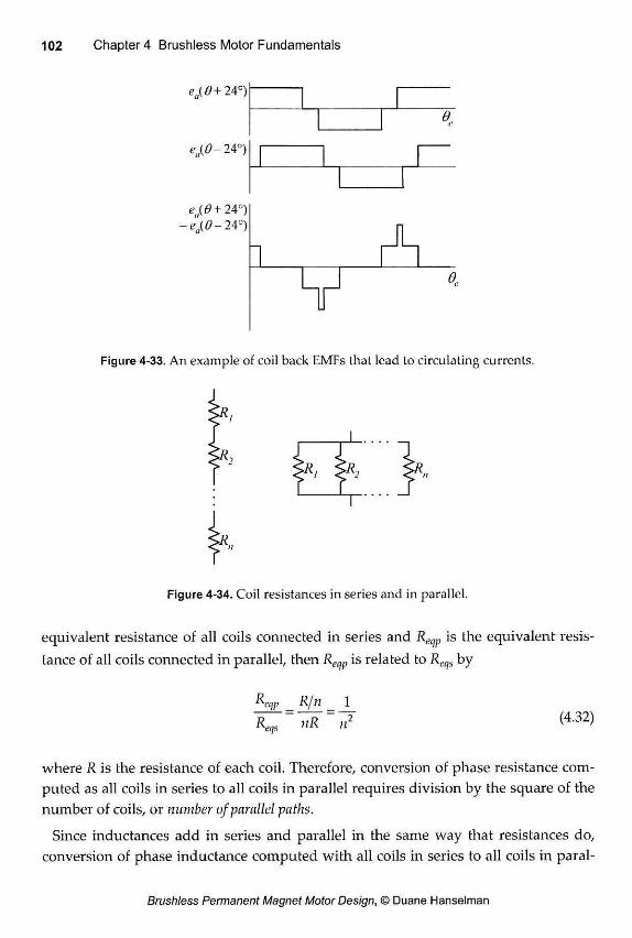
ejL0+ 24°)

ea{6-24°)

e„(0+24°) -eAO- 24°)

1

Figure 4-33. An example of coil back EMFs that lead to circulating currents.

>R,

>R->R, <R2

>R.

Figure 4-34. Coil resistances in series and in parallel.

equivalent resistance of all coils connected in series and Reqp is the equivalent resis-tance of all coils connected in parallel, then Reqp is related to RecjS by

R. cqp _ R/n _ 1 R. eqs

TIR (4.32)

where R is the resistance of each coil. Therefore, conversion of phase resistance com-puted as all coils in series to all coils in parallel requires division by the square of the number of coils, or number of parallel paths.

Since inductances add in series and parallel in the same way that resistances do, conversion of phase inductance computed with all coils in series to all coils in paral-

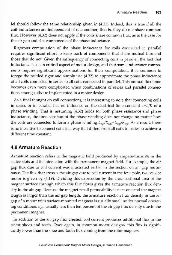
lei should follow the same relationship given in (4.32). Indeed, this is true if all the coil inductances are independent of one another; that is, they do not share common flux. However (4.32) does not apply if the coils share common flux, as is the case for the air gap and slot components of the phase inductance.

Rigorous computation of the phase inductance for coils connected in parallel requires significant effort to keep track of components that share mutual flux and those that do not. Given the infrequency of connecting coils in parallel, the fact that inductance is a less critical aspect of motor design, and that some inductance compo-nents require significant approximations for their computation, it is common to forego the needed rigor and simply use (4.32) to approximate the phase inductance of all coils connected in series to all coils connected in parallel. This mutual flux issue becomes even more complicated when combinations of series and parallel connec-tions among coils are implemented in a motor design.

As a final thought on coil connections, it is interesting to note that connecting coils in series or in parallel has no influence on the electrical time constant r=L/R of a phase winding. That is, assuming (4.32) holds for both phase resistance and phase inductance, the time constant of the phase winding does not change no matter how the coils are connected to form a phase winding LeCjS/RC(jS=Letjp/Reqr. As a result, there is no incentive to connect coils in a way that differs from all coils in series to achieve a different time constant.

4.8 Armature Reaction

Armature reaction refers to the magnetic field produced by ampere-turns Ni in the stator slots and its interaction with the permanent magnet field. For example, the air gap flux due to coil current was illustrated earlier in the section on air gap induc-tance. The flux that crosses the air gap due to coil current in the four pole, twelve slot motor is given by (4.19). Dividing this expression by the cross-sectional area of the magnet surface through which this flux flows gives the armature reaction flux den-sity in the air gap. Because the magnet recoil permeability is near one and the magnet length is larger than the air gap length, the armature reaction flux density in the air gap of a motor with surface-mounted magnets is usually small under normal operat-ing conditions, e.g., usually less than ten percent of the air gap flux density due to the permanent magnet.

In addition to the air gap flux created, coil current produces additional flux in the stator shoes and teeth. Once again, in common motor designs, this flux is signifi-cantly lower than the shoe and tooth flux coming from the rotor magnets.

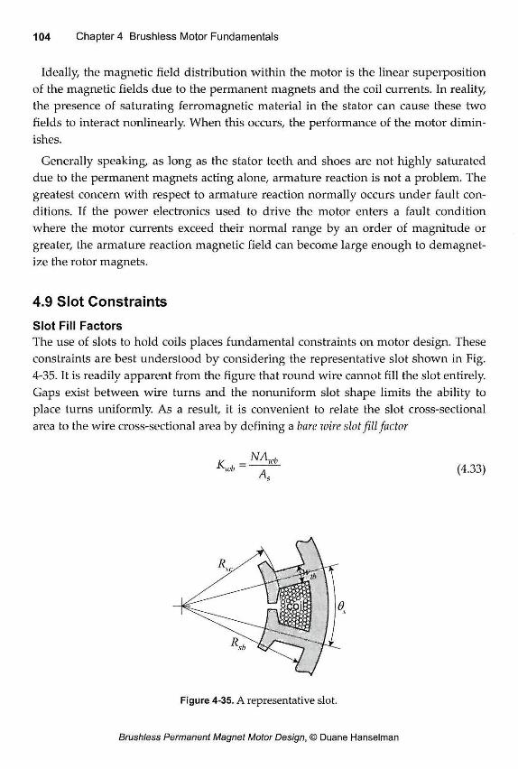
Ideally; the magnetic field distribution within the motor is the linear superposition of the magnetic fields due to the permanent magnets and the coil currents. In reality, the presence of saturating ferromagnetic material in the stator can cause these two fields to interact nonlinearly. When this occurs, the performance of the motor dimin-ishes.

Generally speaking, as long as the stator teeth and shoes are not highly saturated due to the permanent magnets acting alone, armature reaction is not a problem. The greatest concern with respect to armature reaction normally occurs under fault con-ditions. If the power electronics used to drive the motor enters a fault condition where the motor currents exceed their normal range by an order of magnitude or greater, the armature reaction magnetic field can become large enough to demagnet-ize the rotor magnets.

4.9 Slot Constraints

Slot Fill Factors The use of slots to hold coils places fundamental constraints on motor design. These constraints are best understood by considering the representative slot shown in Fig. 4-35. It is readily apparent from the figure that round wire cannot fill the slot entirely. Gaps exist between wire turns and the nonuniform slot shape limits the ability to place turns uniformly. As a result, it is convenient to relate the slot cross-sectional area to the wire cross-sectional area by defining a bare wire slot fill factor

Kb - ~7 (4.33)

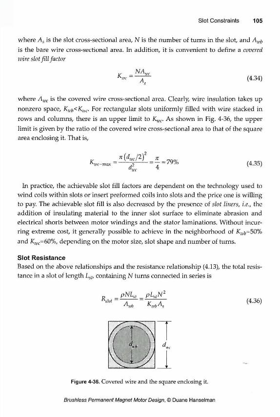
where As is the slot cross-sectional area, N is the number of turns in the slot, and Au,b

is the bare wire cross-sectional area. In addition, it is convenient to define a covered wire slot fill factor

NAU!C

(4.34) K = UK

where Awc is the covered wire cross-sectional area. Clearly, wire insulation takes up nonzero space, Kwb<Kwc. For rectangular slots uniformly filled with wire stacked in rows and columns, there is an upper limit to Kwc. As shown in Fig. 4-36, the upper limit is given by the ratio of the covered wire cross-sectional area to that of the square area enclosing it. That is,

K, K*/2) 3 79% (4.35)

In practice, the achievable slot fill factors are dependent on the technology used to wind coils within slots or insert preformed coils into slots and the price one is willing to pay. The achievable slot fill is also decreased by the presence of slot liners, i.e., the addition of insulating material to the inner slot surface to eliminate abrasion and electrical shorts between motor windings and the stator laminations. Without incur-ring extreme cost, it generally possible to achieve in the neighborhood of Kwb=50% and Ku,c=60%, depending on the motor size, slot shape and number of turns.

Slot Resistance Based on the above relationships and the resistance relationship (4.13), the total resis-tance in a slot of length Lst, containing N turns connected in series is

Klot = PNLst PLstN< A I db Kw bA s

(4.36)

Figure 4-36. Covered wire and the square enclosing it.

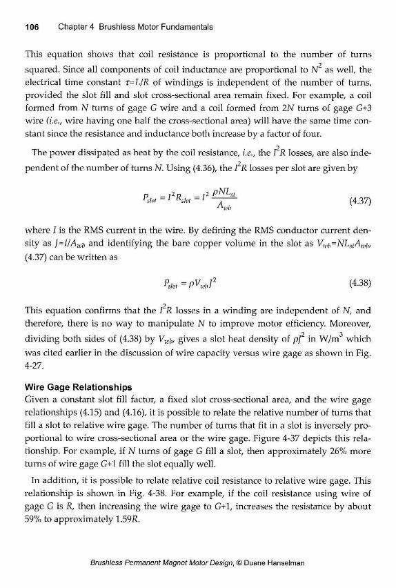
This equation shows that coil resistance is proportional to the number of turns squared. Since all components of coil inductance are proportional to N as well, the electrical time constant r=L/R of windings is independent of the number of turns, provided the slot fill and slot cross-sectional area remain fixed. For example, a coil formed from N turns of gage G wire and a coil formed from 2N turns of gage G+3 wire (i.e., wire having one half the cross-sectional area) will have the same time con-stant since the resistance and inductance both increase by a factor of four.

2 The power dissipated as heat by the coil resistance, i.e., the I R losses, are also inde-

pendent of the number of turns N. Using (4.36), the I R losses per slot are given by

P - j2n _ ,2 pNLst

'slot-1 slot - 1 A ^ (4.37)

where I is the RMS current in the wire. By defining the RMS conductor current den-sity as ]=I/Awb and identifying the bare copper volume in the slot as Vwh=NLstAwiu

(4.37) can be written as

Psiot = PKJ2 (4-38)

This equation confirms that the I~R losses in a winding are independent of N, and therefore, there is no way to manipulate N to improve motor efficiency. Moreover,

2 3

dividing both sides of (4.38) by Vwi„ gives a slot heat density of p/ in W/m which was cited earlier in the discussion of wire capacity versus wire gage as shown in Fig. 4-27. Wire Gage Relationships Given a constant slot fill factor, a fixed slot cross-sectional area, and the wire gage relationships (4.15) and (4.16), it is possible to relate the relative number of turns that fill a slot to relative wire gage. The number of turns that fit in a slot is inversely pro-portional to wire cross-sectional area or the wire gage. Figure 4-37 depicts this rela-tionship. For example, if N turns of gage G fill a slot, then approximately 26% more turns of wire gage G+l fill the slot equally well.

In addition, it is possible to relate relative coil resistance to relative wire gage. This relationship is shown in Fig. 4-38. For example, if the coil resistance using wire of gage G is R, then increasing the wire gage to G+l, increases the resistance by about 59% to approximately 1.59R.

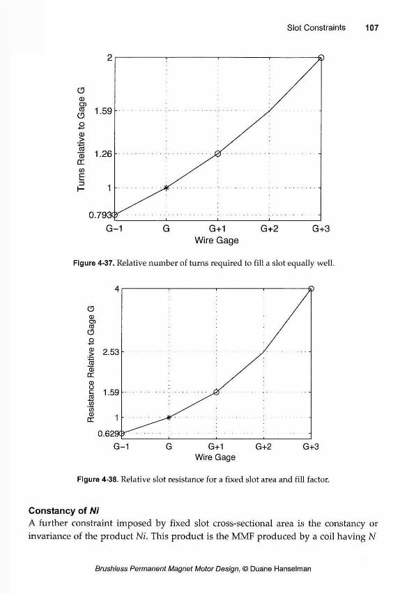
Wire Gage

Figure 4-37. Relative number of turns required to fill a slot equally well.

Wire Gage

Figure 4-38. Relative slot resistance for a fixed slot area and fill factor.

Constancy of Ni

A further constraint imposed by fixed slot cross-sectional area is the constancy or invariance of the product Ni. This product is the MMF produced by a coil having N

turns, each carrying a current of i. Based on the bare wire slot fill factor (4.33) and the current density relationship, the product Ni is equal to

This equation shows that Ni is a constant set by the bare wire slot fill factor and the slot current density. When N increases by some factor, the wire cross-sectional area and resulting current decrease by the same factor. The constancy of Ni implies that neither N nor i can be changed independently to maximize torque as given by (4.8).

4.10 Torque Constant, Back EMF Constant, and Motor Constant

The specification sheets for brushless permanent magnet motors often cite values for the torque constant Kt=T/i and the back EMF constant Ke=Eh/(om, but few provide val-ues for the motor constant Km. Of these specifications, the torque constant is gener-ally the least useful and most deceiving. At first glance it appears that a larger torque constant means that more torque can be obtained for the same amount of current. However, for a given rotor and stator, the constancy of Ni implies that this is not true. Increasing the torque constant by increasing N does not increase the torque capabil-ity of a motor since any increase in N forces the current i to decrease correspondingly.

In the selection of a motor, the back EMF constant is generally more useful because it does not involve the current i. For a given rotor and stator, the back EMF constant scales linearly with N. As a result, by winding the motor with different gage wires and keeping the slot fill factor constant, smaller diameter wires make room for greater numbers of turns N. As a result, different back EMF constants are obtained. Therefore, in practice, the back EMF constant and rated application speed are used to set the peak back EMF voltage to some level just under the voltage available from the power electronics used to drive the motor. Once the back EMF constant is deter-mined by the power electronics, the torque constant is set because of their equiva-lence as given in (4.9). (Note that motor specification sheets do not demonstrate this equivalence because the torque constant and back EMF constants are specified using inconsistent conditions and inconsistent units.)

Since the torque constant and back EMF constant vary with N and the product Ni is constant, they are not good indicators of motor performance. A more useful perform-ance indicator is motor constant, which is defined as

Ni = NAwbJ = KwbAs] (4.39)

T (4.40)

Torque Constant, Back EMF Constant, and Motor Constant 109

As stated, the motor constant expresses torque efficiency, which is different from power efficiency. Motor constant describes how efficiently a motor produces torque as a function of the I R losses incurred in the production of that torque. That is, motor constant is related not only to the desired motor output, but is also inversely proportional to the cost of producing that output.

Since torque is proportional to current and power is proportional to current squared, using the square root of power in (4.40) allows current to cancel from the ratio. As a result, motor constant is independent of current and the number of turns N, and remains unchanged as long as the slot fill factor is fixed. Therefore, motor constant provides a good indication of motor performance.

To illustrate these facts, consider the ideal torque produced by one coil filling two slots as given in (4.8) and having twice the total resistance of one slot (4.36). Substi-tuting these expressions into (4.40) and simplifying gives

_2NBgLstR„I _ 2 NBsLstRro _ BgRn

m " ^ Z ) - J2PLstN/Awb - V (4-41)

where Vn,b is the bare wire volume contained in the two slots. This result confirms that the motor constant is independent of number of turns N as well as current. A family of motors constructed from a given rotor and stator will produce torque with equal efficiency as long as the total volume of bare wire remains unchanged. As N increases, the torque per ampere (i.e., torque constant) increases, but simultaneously the resistance increases with the square of N, so the motor constant is unchanged.

Torque efficiency as described by (4.41) is proportional to the air gap flux density, the rotor outside radius, and the square root of the wire volume. The air gap flux density can be increased by decreasing the air gap length, increasing the magnet length, (both of which imply increasing the permeance coefficient) or by using a more powerful magnet. The air gap length can only be decreased so far before manu-facturing tolerances make it impossible to maintain a consistent air gap. Therefore, once the air gap is minimized, one must buy more magnet material or buy more powerful magnet material to increase torque efficiency.

Increasing the rotor outside radius increases the motor constant but requires that the stator diameter increase to maintain the wire volume. If the stator diameter is constant, increasing the rotor outside radius has little affect on the motor constant. If the rotor outside radius is fixed, increasing the wire volume means increasing the outside stator diameter or increasing the slot fill factor. Increasing the slot fill factor

alone is usually difficult because it becomes increasingly expensive to pack more and more wire into slots, especially as one gets closer to the theoretical maximum.

4.11 Torque per Unit Rotor Volume

In Chapter 1, it was argued that torque is proportional to rotor volume as stated in (1.8) as T=kD L. In this expression k is the only unknown. For a given rotor volume, its value determines the quality of a motor design. Rather than try to determine k specifically, it is beneficial to determine the torque produced per unit rotor volume. To do so, consider the torque produced by the motor shown in Fig. 4-11, whose phase torque is given by (4.11). Based on (4.11) the torque per unit rotor volume is

|T| _ 2NmBgNi TRV ~ n 2 r ~ n (4.42) JcRtUt nRrn K >

This expression is directly proportional to k in (1.8). For a fixed air gap radius Rro, the torque produced per unit rotor volume is directly proportional to the air gap flux density Bg, the number of magnet poles Nm, and the coil ampere-turns Ni. If the sta-tor volume is fixed, Ni is a constant, thereby making Nm and Bg responsible for maxi-mizing the torque per unit rotor volume. As with the motor constant, the air gap flux density plays a crucial role in determining performance. Increasing Bg means decreasing the air gap length, or increasing the quality or quantity of magnet mate-rial used.

The torque per unit rotor volume describes the amount of torque available from a given rotor volume. As such, it is a common measure for comparing motors and for initial motor sizing for a given application. Even more common is the use of the air gap shear stress, which is the tangential force per unit rotor surface area. This meas-ure is often easier to visualize and is very simply related to the torque per unit rotor volume. Using (1.1) and (4.11), the air gap shear stress is given by

F NmBgNI ^ Ktrv

a~2nRroLst~ kRw ~ 2 ( 4 - 4 3 )

While this expression applies to the ideal conditions implied by (4.11), the air gap shear stress provides a useful comparative measure. Often the air gap shear stress is

2 expressed in lbf/in (psi). When expressed in these units, low cost brushiess perma-

nent magnet motors typically exhibit a shear stress in the range 0.5<a<2, higher cost motors are in the range 1.5<G<3, very high performance motors are typically in the range 2<a<10, and large liquid cooled motors can be in the range 10<a<20. From (4.43) it is clear that the number of magnet poles, the air gap flux density, and the coil ampere turns Ni are important quantities. In low performance motors, these values are compromised to reduce cost, whereas in high performance motors, they are pushed to achieve performance.

4.12 Cogging Torque

As described in Chapter 1 and illustrated in Figs. 1-6 and 1-7, cogging torque describes the interaction of the rotor magnets acting on the stator teeth or poles inde-pendent of any current. Mathematically this torque was described as part of the gen-eral torque expression (3.37). While this torque is often considered beneficial in step motors, it is considered detrimental in brushless permanent magnet motors.

This dissatisfaction with cogging torque often lacks quantitative support. One of the first things engineers invariably do when they pick up a small motor is to spin the shaft with their fingers. The pulsations felt during this process are caused by cog-ging torque. In comparing several motors based on this qualitative examination, engineers will judge the one with the least cogging torque the best, even if it per-forms the worst in the actual motor application.

In reality, cogging torque is often very small relative to the beneficial mutual torque produced by a motor. Furthermore, even a slight mismatch between the back EMF of the motor and the motor current often produces greater ripple torque than the cog-ging torque itself. In this situation, cogging torque is masked by the larger torque variation in the mutual torque. As a result, the qualitative shaft spin test is often mis-leading.

Despite the insignificance of cogging torque in many applications and in the pres-ence of mutual torque ripple due to back EMF-current mismatch, cogging torque is a motor characteristic worth understanding. Simply put, cogging torque is the torque created when the rotor permanent magnets attempt to align themselves with a maxi-mum amount of ferromagnetic material. This is visually obvious for simple struc-tures such as that shown in Fig. 1-6, but is more difficult to visualize for common motor structures despite the fact that the same fundamental phenomenon is occur-ring.

To understand cogging torque, consider the cogging torque term from (3.37)

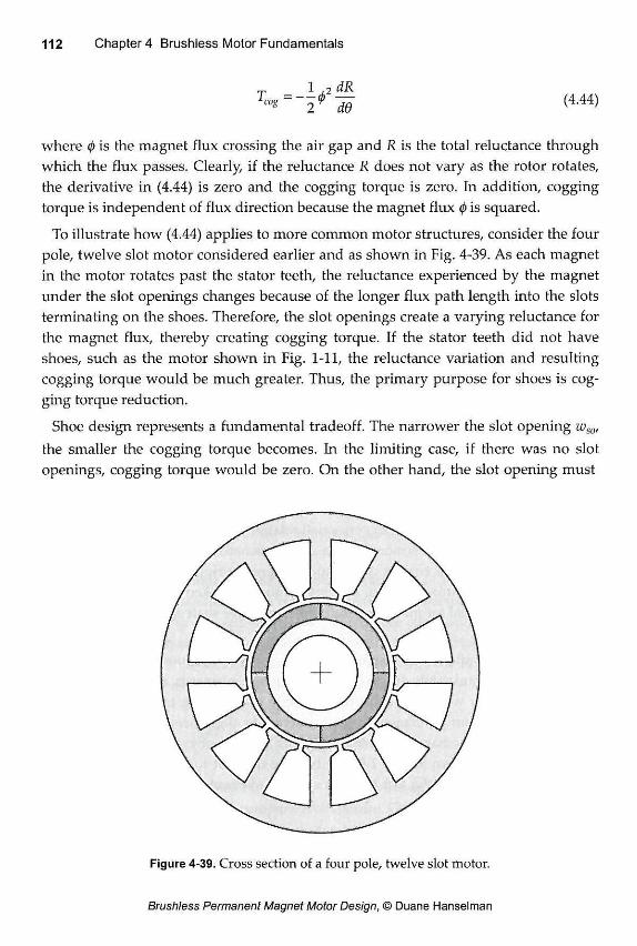
(4.44)

where (p is the magnet flux crossing the air gap and R is the total reluctance through which the flux passes. Clearly, if the reluctance R does not vary as the rotor rotates, the derivative in (4.44) is zero and the cogging torque is zero. In addition, cogging torque is independent of flux direction because the magnet flux 0 is squared.

To illustrate how (4.44) applies to more common motor structures, consider the four pole, twelve slot motor considered earlier and as shown in Fig. 4-39. As each magnet in the motor rotates past the stator teeth, the reluctance experienced by the magnet under the slot openings changes because of the longer flux path length into the slots terminating on the shoes. Therefore, the slot openings create a varying reluctance for the magnet flux, thereby creating cogging torque. If the stator teeth did not have shoes, such as the motor shown in Fig. 1-11, the reluctance variation and resulting cogging torque would be much greater. Thus, the primary purpose for shoes is cog-ging torque reduction.

Shoe design represents a fundamental tradeoff. The narrower the slot opening wso, the smaller the cogging torque becomes. In the limiting case, if there was no slot openings, cogging torque would be zero. On the other hand, the slot opening must

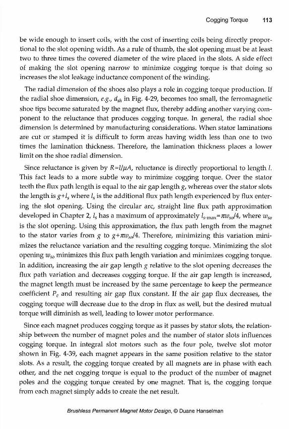
be wide enough to insert coils, with the cost of inserting coils being directly propor-tional to the slot opening width. As a rule of thumb, the slot opening must be at least two to three times the covered diameter of the wire placed in the slots. A side effect of making the slot opening narrow to minimize cogging torque is that doing so increases the slot leakage inductance component of the winding.

The radial dimension of the shoes also plays a role in cogging torque production. If the radial shoe dimension, e.g., dsb in Fig. 4-29, becomes too small, the ferromagnetic shoe tips become saturated by the magnet flux, thereby adding another varying com-ponent to the reluctance that produces cogging torque. In general, the radial shoe dimension is determined by manufacturing considerations. When stator laminations are cut or stamped it is difficult to form areas having width less than one to two times the lamination thickness. Therefore, the lamination thickness places a lower limit on the shoe radial dimension.

Since reluctance is given by R=l//iA, reluctance is directly proportional to length I. This fact leads to a more subtle way to minimize cogging torque. Over the stator teeth the flux path length is equal to the air gap length g, whereas over the stator slots the length is g+ls where ls is the additional flux path length experienced by flux enter-ing the slot opening. Using the circular arc, straight line flux path approximation developed in Chapter 2, LS has a maximum of approximately LS.MAX= TUOSJ4, where zvso

is the slot opening. Using this approximation, the flux path length from the magnet to the stator varies from g to g+mvso/4. Therefore, minimizing this variation mini-mizes the reluctance variation and the resulting cogging torque. Minimizing the slot opening wso minimizes this flux path length variation and minimizes cogging torque. In addition, increasing the air gap length g relative to the slot opening decreases the flux path variation and decreases cogging torque. If the air gap length is increased, the magnet length must be increased by the same percentage to keep the permeance coefficient Pc and resulting air gap flux constant. If the air gap flux decreases, the cogging torque will decrease due to the drop in flux as well, but the desired mutual torque will diminish as well, leading to lower motor performance.

Since each magnet produces cogging torque as it passes by stator slots, the relation-ship between the number of magnet poles and the number of stator slots influences cogging torque. In integral slot motors such as the four pole, twelve slot motor shown in Fig. 4-39, each magnet appears in the same position relative to the stator slots. As a result, the cogging torque created by all magnets are in phase with each other, and the net cogging torque is equal to the product of the number of magnet poles and the cogging torque created by one magnet. That is, the cogging torque from each magnet simply adds to create the net result.

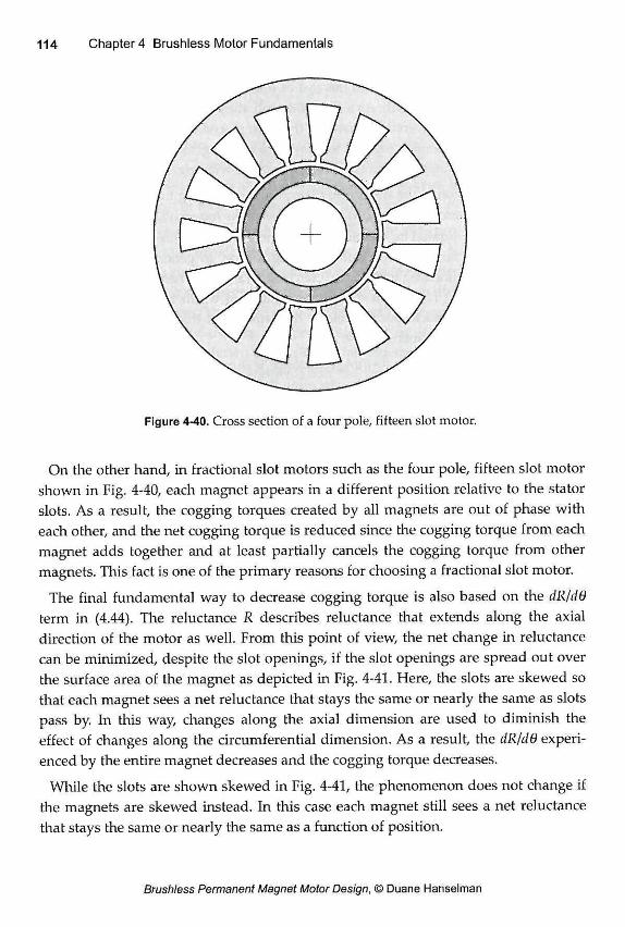
On the other hand, in fractional slot motors such as the four pole, fifteen slot motor shown in Fig. 4-40, each magnet appears in a different position relative to the stator slots. As a result, the cogging torques created by all magnets are out of phase with each other, and the net cogging torque is reduced since the cogging torque from each magnet adds together and at least partially cancels the cogging torque from other magnets. This fact is one of the primary reasons for choosing a fractional slot motor.

The final fundamental way to decrease cogging torque is also based on the dR/dd term in (4.44). The reluctance R describes reluctance that extends along the axial direction of the motor as well. From this point of view, the net change in reluctance can be minimized, despite the slot openings, if the slot openings are spread out over the surface area of the magnet as depicted in Fig. 4-41. Here, the slots are skewed so that each magnet sees a net reluctance that stays the same or nearly the same as slots pass by. In this way, changes along the axial dimension are used to diminish the effect of changes along the circumferential dimension. As a result, the dR/dO experi-enced by the entire magnet decreases and the cogging torque decreases.

While the slots are shown skewed in Fig. 4-41, the phenomenon does not change if the magnets are skewed instead. In this case each magnet still sees a net reluctance that stays the same or nearly the same as a function of position.

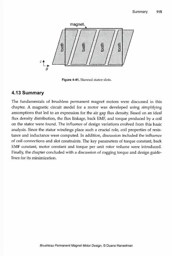
Figure 4-41. Skewed stator slots.

4.13 Summary

The fundamentals of brushless permanent magnet motors were discussed in this chapter. A magnetic circuit model for a motor was developed using simplifying assumptions that led to an expression for the air gap flux density. Based on an ideal flux density distribution, the flux linkage, back EMF, and torque produced by a coil on the stator were found. The influence of design variations evolved from this basic analysis. Since the stator windings place such a crucial role, coil properties of resis-tance and inductance were computed. In addition, discussion included the influence of coil connections and slot constraints. The key parameters of torque constant, back EMF constant, motor constant and torque per unit rotor volume were introduced. Finally, the chapter concluded with a discussion of cogging torque and design guide-lines for its minimization.

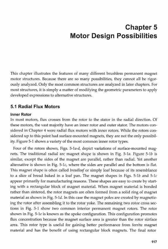
This chapter illustrates the features of many different brushless permanent magnet motor structures. Because there are so many possibilities, they cannot all be rigor-ously analyzed. Only the most common structures are analyzed in later chapters. For most structures, it is simply a matter of modifying the geometric parameters to apply developed expressions to alternative structures.

5.1 Radial Flux Motors

Inner Rotor In most motors, flux crosses from the rotor to the stator in the radial direction. Of these motors, the vast majority have an inner rotor and outer stator. The motors con-sidered in Chapter 4 were radial flux motors with inner rotors. While the rotors con-sidered up to this point had surface-mounted magnets, they are not the only possibil-ity. Figure 5-1 shows a variety of the most common inner rotor types.

Four of the rotors shown, Figs. 5-\a-d, depict variations of surface-mounted mag-nets. The traditional radial arc magnet shape is shown in Fig. 5-1«. Figure 5-lb is similar, except the sides of the magnet are parallel, rather than radial. Yet another alternative is shown in Fig. 5-lc, where the sides are parallel and the bottom is flat. This magnet shape is often called breadloaf or simply loaf because of its resemblance to a slice of bread baked in a loaf pan. The magnet shapes in Figs. 5-1 b and 5-lc appear primarily for manufacturing reasons. These shapes are easy to create by start-ing with a rectangular block of magnet material. When magnet material is bonded rather than sintered, the rotor magnets are often formed from a solid ring of magnet material as shown in Fig. 5-Id. In this case the magnet poles are created by magnetiz-ing the rotor after assembling it to the rotor yoke. The remaining two rotor cross sec-tions in Fig. 5-1 show two common interior permanent magnet rotors. The rotor shown in Fig. 5-le is known as the spoke configuration. This configuration promotes flux concentration because the magnet surface area is greater than the rotor surface area. This rotor type is useful for gaining better performance from ferrite magnet material and has the benefit of using rectangular block magnets. The final rotor

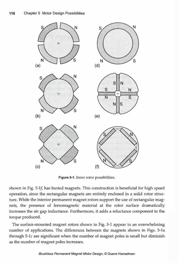
Figure 5-1. Inner rotor possibilities.

shown in Fig. 5-1/, has buried magnets. This construction is beneficial for high speed operation, since the rectangular magnets are entirely enclosed in a solid rotor struc-ture. While the interior permanent magnet rotors support the use of rectangular mag-nets, the presence of ferromagnetic material at the rotor surface dramatically increases the air gap inductance. Furthermore, it adds a reluctance component to the torque produced.

The surface-mounted magnet rotors shown in Fig. 5-1 appear in an overwhelming number of applications. The differences between the magnets shown in Figs. 5-la through 5-lc are significant when the number of magnet poles is small but diminish as the number of magnet poles increases.

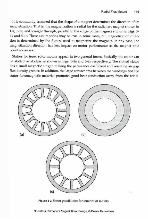
It is commonly assumed that the shape of a magnet determines the direction of its magnetization. That is, the magnetization is radial for the radial arc magnet shown in Fig. 5-1 a, and straight through, parallel to the edges of the magnets shown in Figs. 5-1 b and 5-lc. These assumptions may be true in some cases, but magnetization direc-tion is determined by the fixture used to magnetize the magnets. In any case, the magnetization direction has less impact on motor performance as the magnet pole count increases.

Stators for inner rotor motors appear in two general forms. Basically, the stator can be slotted or slotless as shown in Figs. 5-2a and 5-2b respectively. The slotted stator has a small magnetic air gap making the permeance coefficient and resulting air gap flux density greater. In addition, the large contact area between the windings and the stator ferromagnetic material promotes good heat conduction away from the wind-

ings to the outer stator surface where it can easily be removed. Cogging torque and the cost of inserting windings through small slot openings are the disadvantages of the slotted stator.

In the slotless stator as shown in Fig. 5-2b, windings are formed into a ring that fits inside the stator yoke and separated from the rotor by a small physical air gap. This construction exhibits no cogging torque since the reluctance seen by the rotor mag-nets does not vary with position. More room exists for windings in the slotless motor, but the reduced thermal conductivity to the outer stator surface reduces the allow-able current density in the windings. In the slotless case, the magnetic air gap encom-passes the physical air gap as well as the radial thickness of the windings. This drives the permeance coefficient and air gap flux density down unless one dramatically increases the quality or quantity of magnet material. As a result, the performance of a motor using slotless stator construction is almost always significantly lower than that of an otherwise equivalent motor having a slotted stator.

The stator shown in Fig. 5-2c has no slot openings. Rather, the stator teeth are con-nected or bridged at the inner radius and end at the outer stator yoke. This construc-tion makes it easier to wind the motor because the windings are inserted over the sta-tor teeth from the outside rather than being inserted through small slot openings from the inside. After the windings are inserted, the stator is inserted into a tight-fitting stator yoke. To gain this manufacturing advantage, this construction suf-fers magnetically. The bridged slot openings increase the slot leakage inductance greatly. In addition, they divert some flux away from the coils reducing the coil flux linkage and resulting back EMF. Moreover, a small air gap is introduced where the teeth meet the stator yoke. To minimize the impact of the bridged slot openings, the radial dimension of the bridge must be made as small as manufacturing will allow. Furthermore, the toothed assembly must fit tightly and concentrically within the outer stator yoke.

Outer Rotor There are several reasons for the overwhelming prevalence of motors having inner rotors. These reasons include the ease of heat removal, because the windings are on the outside, and the containment of the rotating element. In some applications, these attributes are not as important as the benefits gained from having an outer rotor and inner stator, such as that shown in Fig. 5-3. Motors having this construction are some-times called inside-out motors. Outer rotor motors appear most commonly as spindle motors for hard disk drives and as the drive motor for ventilation fans, such as those used to cool CPUs and computer cases. In these applications, the motor becomes an integrated part of a larger structure.

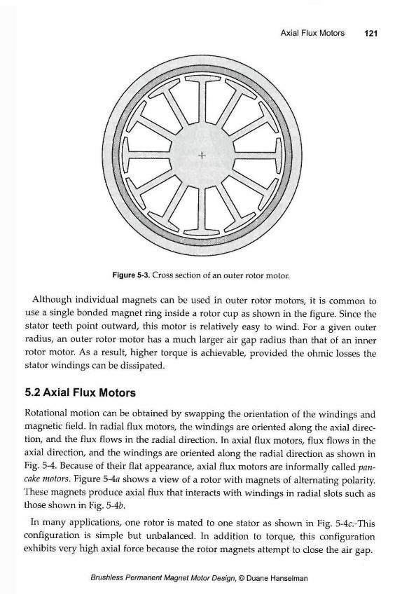
Although individual magnets can be used in outer rotor motors, it is common to use a single bonded magnet ring inside a rotor cup as shown in the figure. Since the stator teeth point outward, this motor is relatively easy to wind. For a given outer radius, an outer rotor motor has a much larger air gap radius than that of an inner rotor motor. As a result, higher torque is achievable, provided the ohmic losses the stator windings can be dissipated.

5.2 Axial Flux Motors

Rotational motion can be obtained by swapping the orientation of the windings and magnetic field. In radial flux motors, the windings are oriented along the axial direc-tion, and the flux flows in the radial direction. In axial flux motors, flux flows in the axial direction, and the windings are oriented along the radial direction as shown in Fig. 5-4. Because of their flat appearance, axial flux motors are informally called pan-cake motors. Figure 5-4« shows a view of a rotor with magnets of alternating polarity. These magnets produce axial flux that interacts with windings in radial slots such as those shown in Fig. 5-4b.

In many applications, one rotor is mated to one stator as shown in Fig. 5-4c. -This configuration is simple but unbalanced. In addition to torque, this configuration exhibits very high axial force because the rotor magnets attempt to close the air gap.

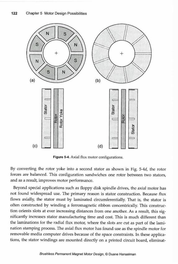
(c)

t

s <0 0> 55 -X

o o > i ~ o u. m S 'S er

(d)

Figure 5-4. Axial flux motor configurations.

By converting the rotor yoke into a second stator as shown in Fig. 5-4d, the rotor forces are balanced. This configuration sandwiches one rotor between two stators, and as a result, improves motor performance.

Beyond special applications such as floppy disk spindle drives, the axial motor has not found widespread use. The primary reason is stator construction. Because flux flows axially, the stator must by laminated circuinferentially. That is, the stator is often constructed by winding a ferromagnetic ribbon concentrically This construc-tion orients slots at ever increasing distances from one another. As a result, this sig-nificantly increases stator manufacturing time and cost. This is much different than the laminations for the radial flux motor, where the slots are cut as part of the lami-nation stamping process. The axial flux motor has found use as the spindle motor for removable media computer drives because of the space constraints. In these applica-tions, the stator windings are mounted directly on a printed circuit board, eliminat-

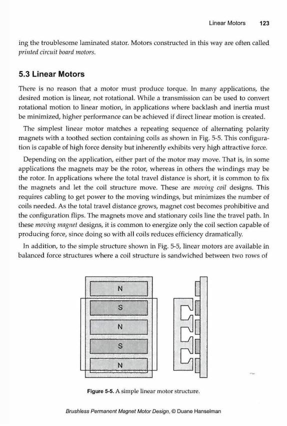
ing the troublesome laminated stator. Motors constructed in this way are often called printed circuit board motors.

5.3 Linear Motors

There is no reason that a motor must produce torque. In many applications, the desired motion is linear, not rotational. While a transmission can be used to convert rotational motion to linear motion, in applications where backlash and inertia must be minimized, higher performance can be achieved if direct linear motion is created.

The simplest linear motor matches a repeating sequence of alternating polarity magnets with a toothed section containing coils as shown in Fig. 5-5. This configura-tion is capable of high force density but inherently exhibits very high attractive force.

Depending on the application, either part of the motor may move. That is, in some applications the magnets may be the rotor, whereas in others the windings may be the rotor. In applications where the total travel distance is short, it is common to fix the magnets and let the coil structure move. These are moving coil designs. This requires cabling to get power to the moving windings, but minimizes the number of coils needed. As the total travel distance grows, magnet cost becomes prohibitive and the configuration flips. The magnets move and stationary coils line the travel path. In these moving magnet designs, it is common to energize only the coil section capable of producing force, since doing so with all coils reduces efficiency dramatically.

In addition, to the simple structure shown in Fig. 5-5, linear motors are available in balanced force structures where a coil structure is sandwiched between two rows of

Figure 5-5. A simple linear motor structure.

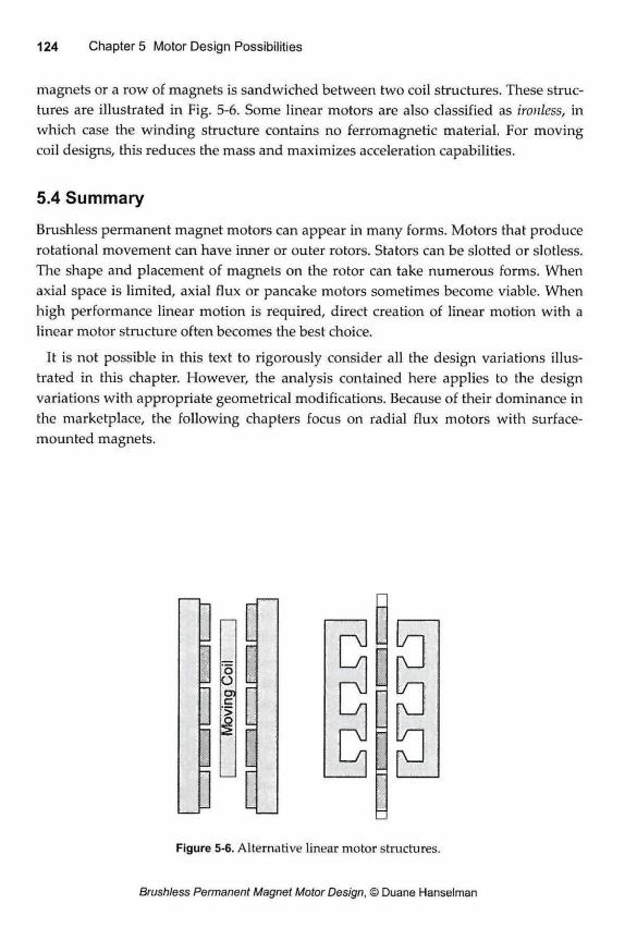
magnets or a row of magnets is sandwiched between two coil structures. These struc-tures are illustrated in Fig. 5-6. Some linear motors are also classified as ironless, in which case the winding structure contains no ferromagnetic material. For moving coil designs, this reduces the mass and maximizes acceleration capabilities.

5.4 Summary

Brushless permanent magnet motors can appear in many forms. Motors that produce rotational movement can have inner or outer rotors. Stators can be slotted or slotless. The shape and placement of magnets on the rotor can take numerous forms. When axial space is limited, axial flux or pancake motors sometimes become viable. When high performance linear motion is required, direct creation of linear motion with a linear motor structure often becomes the best choice.

It is not possible in this text to rigorously consider all the design variations illus-trated in this chapter. However, the analysis contained here applies to the design variations with appropriate geometrical modifications. Because of their dominance in the marketplace, the following chapters focus on radial flux motors with surface-mounted magnets.

Figure 5-6. Alternative linear motor structures.

Brushless permanent magnet motors can have any even number of magnet poles Nm

and any number of slots Ns. From this infinite set, only a small number of magnet pole and slot count combinations maximize use of the stator slots and lead to effi-cient torque production. This chapter develops the concepts required to identify these valid pole and slot count combinations for three phase motors. In addition, this chapter presents a procedure for determining the winding layout for any valid pole and slot combination.

6.1 Assumptions

Since there are an infinite number of possibilities for pole and slot count combina-tions and for winding layouts, assumptions are required to focus or limit the scope so that desirable windings can be found. The assumptions considered here are:

a) The motor has three phases. (Modification of the material in this chapter for other phase counts follows in a straightforward fashion).

b) All slots are filled. Therefore the number of slots is a multiple of the number of phases, i.e., Ns=kNpi,. So for three phase motors, the number of slots is always a multiple of three.

c) There are two coil sides in each slot. That is, the winding can be classified as a double layer winding.

d) Only balanced windings are considered. In other words, only pole and slot count combinations that result in the back EMF of phases B and C being 120°E offset from the back EMF of phase A are considered.

e) The number of slots per pole per phase is assumed to be less than or equal to two, where Nspp=NJNm/Nph is the number of slots per pole per phase. This restriction is primarily for convenience. Most motors fulfill this require-ment. If Nspp is greater than two, another degree of freedom is introduced that can complicate the winding layout but seldom if ever increases motor

performance. In practice, Nspp>2 often appears when a stator lamination is reused for a motor having fewer magnet poles.

f) All coils have the same number of turns and all span the same number of slots. This implies that all coils are the same size and therefore have the same resistance and inductance.

Abiding by the above list of assumptions routinely leads to motors that are capable of high performance. Moreover, these assumptions lead to motors that are readily wound. Motors can be wound that violate one or more of these assumptions. How-ever, they may be more difficult to wind or may offer reduced performance.

6.2 Coil Span

As described in Chapter 4, coil span or coil pitch is the circumferential width of a coil. Coil span can be specified in terms of mechanical or electrical measures. In slot-ted motors, it is convenient to describe the coil span in terms of slots. For example, if a coil goes from slot k to slot k+2, the coil span is 2 slots.

Generally speaking, the coil span for a coil should be as close to 180 °E as possible but seldom exceed it. Doing so maximizes the flux linked to the coil and therefore maximizes the back EMF induced in the coil. The exception to this rule occurs when the slot pitch exceeds 180°E. This occurs when the number of slots Ns is less than the number of magnet poles N,„, a condition that appears most often in outer rotor motors. In this case, when the slot pitch exceeds 180°E, the coil pitch is set to the minimum of one.

The nominal coil span as described above, can be found by defining the number of slots per magnet pole as

This value gives the number of slots per 180°E. As a result, the nominal coil span in slots is the integer portion of (6.1), or

S = max fix ±L N„,

,1 (6.2)

where the function max(v) returns the maximum of its two arguments and the func-tion fix(-) returns the integer portion of its argument. The function max(v) is included in (6.2) to insure that the span is at least one slot when Ns<Nm.

Occasionally, the winding span differs from the nominal span given in (6.2). When it does, the span chosen most often is equal to S*-l . Decreasing the span decreases the length of the end turns and changes the amplitude and harmonic content of the flux linkage and resulting back EMF. When this is done, the winding is said to be short pitched or chorded.

6.3 Valid Pole and Slot Combinations

Only certain combinations of magnet poles and stator slots fit the preceding winding assumptions. For example, for three phase motors the number of slots must be a mul-tiple of three, or not all slots will be filled with two coil sides. Before considering the details of laying out a winding, it is beneficial to identify the subset of magnet pole and slot count combinations that lead to valid windings.

For three phase motors, each of the three phase windings must produce a back EMF of the same amplitude and shape. More important here is that each back EMF be shifted in phase by 120°E from the other two phases. When these three criteria on the amplitude, shape, and relative phase are met, the winding is said to be balanced.

The amplitude and shape of the phase back EMFs will be identical if the coils in each phase have the same number of turns and the same coil span and are distrib-uted in the same way around the stator. Since these criteria are met by the winding assumptions, valid pole and slot counts are then determined by the ability to produce the 120°E relative phase offset among the three phase windings.

With reference to Fig. 6-1, if the first coil of phase A uses slot 0 and slot S, where S is the chosen coil span, then the first coil of phase B must use a slot k and k+S, where k is chosen so that slots 0 and k are separated by 120°E. The slots may also be 120°E+ i]360°E apart where q is any integer. That is, the principle angle between slots 0 and k must be 120°E. If no such slot can be found, the chosen pole and slot count combina-tion does not support a balanced winding.

When a slot k is found, each coil in phase B is shifted by k slots with respect to the corresponding coil in phase A. This span of K0= k slots is called the phase offset. For each coil in phase A, each corresponding coil in phase B is shifted K0 slots, thereby assuring that the individual coil back EMFs of phase B are shifted 120°E relative to those of phase A.

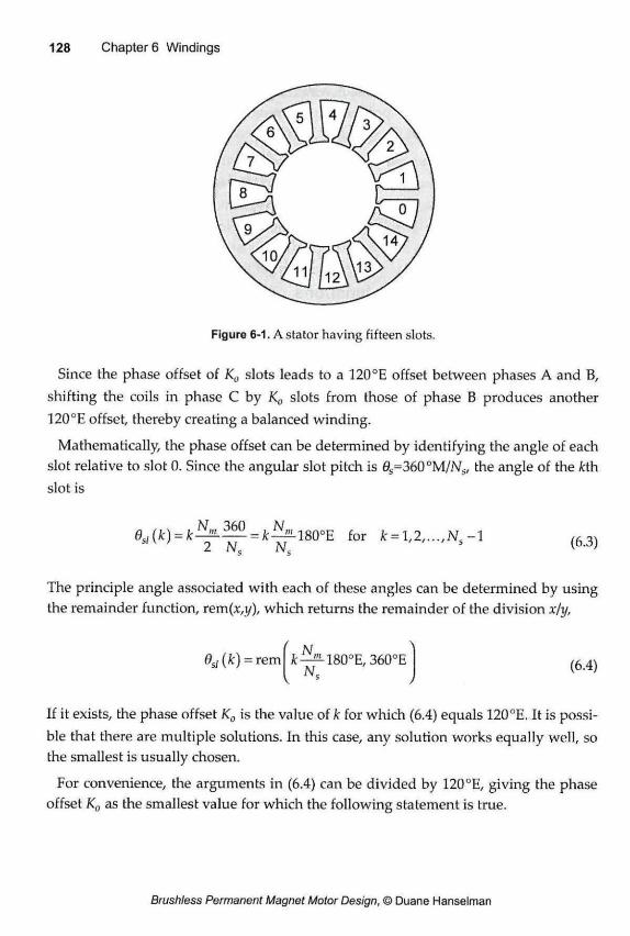
Figure 6-1. A stator having fifteen slots.

Since the phase offset of K0 slots leads to a 120°E offset between phases A and B, shifting the coils in phase C by K0 slots from those of phase B produces another 120°E offset, thereby creating a balanced winding.

Mathematically, the phase offset can be determined by identifying the angle of each slot relative to slot 0. Since the angular slot pitch is 0S=36O°M/NS, the angle of the kih slot is

The principle angle associated with each of these angles can be determined by using the remainder function, rem(x,i/), which returns the remainder of the division x/y,

If it exists, the phase offset K0 is the value of k for which (6.4) equals 120°E. It is possi-ble that there are multiple solutions. In this case, any solution works equally well, so the smallest is usually chosen.

For convenience, the arguments in (6.4) can be divided by 120°E, giving the phase offset K0 as the smallest value for which the following statement is true.

esl(k) = k N m 3 6 0 180°E for A: = 1,2 N - l s n ' 2 N« N 5 (6.3)

(6.4)

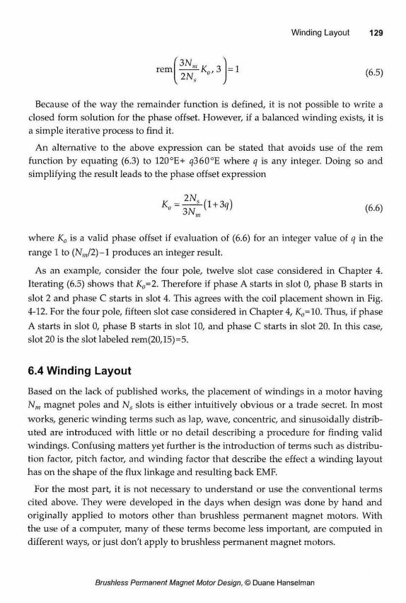
rem =1 /

\

(6.5)

Because of the way the remainder function is defined, it is not possible to write a closed form solution for the phase offset. However, if a balanced winding exists, it is a simple iterative process to find it.

An alternative to the above expression can be stated that avoids use of the rem function by equating (6.3) to 120°E+ i/360°E where q is any integer. Doing so and simplifying the result leads to the phase offset expression

where K0 is a valid phase offset if evaluation of (6.6) for an integer value of q in the range 1 to (N,J2)-l produces an integer result.

As an example, consider the four pole, twelve slot case considered in Chapter 4. Iterating (6.5) shows that K0=2. Therefore if phase A starts in slot 0, phase B starts in slot 2 and phase C starts in slot 4. This agrees with the coil placement shown in Fig. 4-12. For the four pole, fifteen slot case considered in Chapter 4, Ko=10. Thus, if phase A starts in slot 0, phase B starts in slot 10, and phase C starts in slot 20. In this case, slot 20 is the slot labeled rem(20,15)=5.

6.4 Winding Layout

Based on the lack of published works, the placement of windings in a motor having Nm magnet poles and Ns slots is either intuitively obvious or a trade secret. In most works, generic winding terms such as lap, wave, concentric, and sinusoidally distrib-uted are introduced with little or no detail describing a procedure for finding valid windings. Confusing matters yet further is the introduction of terms such as distribu-tion factor, pitch factor, and winding factor that describe the effect a winding layout has on the shape of the flux linkage and resulting back EMF.

For the most part, it is not necessary to understand or use the conventional terms cited above. They were developed in the days when design was done by hand and originally applied to motors other than brushless permanent magnet motors. With the use of a computer, many of these terms become less important, are computed in different ways, or just don't apply to brushless permanent magnet motors.

(6.6)

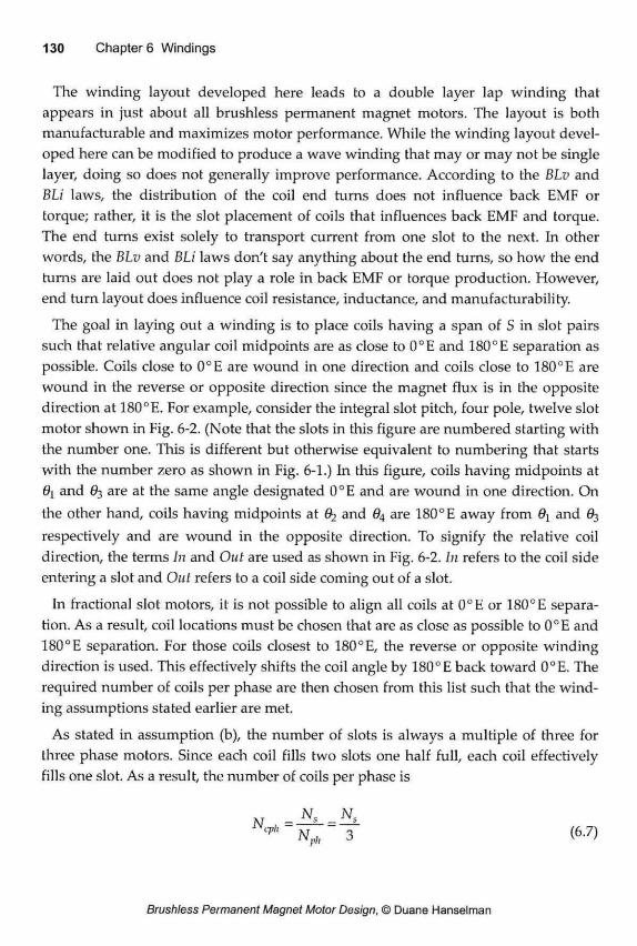
The winding layout developed here leads to a double layer lap winding that appears in just about all brushless permanent magnet motors. The layout is both manufacturable and maximizes motor performance. While the winding layout devel-oped here can be modified to produce a wave winding that may or may not be single layer, doing so does not generally improve performance. According to the BLv and BLi laws, the distribution of the coil end turns does not influence back EMF or torque; rather, it is the slot placement of coils that influences back EMF and torque. The end turns exist solely to transport current from one slot to the next. In other words, the BLv and BLi laws don't say anything about the end turns, so how the end turns are laid out does not play a role in back EMF or torque production. However, end turn layout does influence coil resistance, inductance, and manufacturability.

The goal in laying out a winding is to place coils having a span of S in slot pairs such that relative angular coil midpoints are as close to 0°E and 180°E separation as possible. Coils close to 0°E are wound in one direction and coils close to 180°E are wound in the reverse or opposite direction since the magnet flux is in the opposite direction at 180 °E. For example, consider the integral slot pitch, four pole, twelve slot motor shown in Fig. 6-2. (Note that the slots in this figure are numbered starting with the number one. This is different but otherwise equivalent to numbering that starts with the number zero as shown in Fig. 6-1.) In this figure, coils having midpoints at 6[ and 03 are at the same angle designated 0°E and are wound in one direction. On the other hand, coils having midpoints at ft and <94 are 180°E away from d\ and ft; respectively and are wound in the opposite direction. To signify the relative coil direction, the terms In and Out are used as shown in Fig. 6-2. In refers to the coil side entering a slot and Out refers to a coil side coming out of a slot.

In fractional slot motors, it is not possible to align all coils at 0°E or 180°E separa-tion. As a result, coil locations must be chosen that are as close as possible to 0°E and 180°E separation. For those coils closest to 180°E, the reverse or opposite winding direction is used. This effectively shifts the coil angle by 180° E back toward 0°E. The required number of coils per phase are then chosen from this list such that the wind-ing assumptions stated earlier are met.

As stated in assumption (b), the number of slots is always a multiple of three for three phase motors. Since each coil fills two slots one half full, each coil effectively fills one slot. As a result, the number of coils per phase is

c p " ~ N p h ~ 3 (6-7)

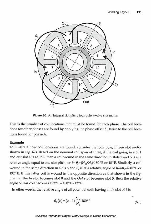
Figure 6-2. An integral slot pitch, four pole, twelve slot motor.

This is the number of coil locations that must be found for each phase. The coil loca-tions for other phases are found by applying the phase offset K0 twice to the coil loca-tions found for phase A.

Example To illustrate how coil locations are found, consider the four pole, fifteen slot motor shown in Fig. 6-3. Based on the nominal coil span of three, if the coil going in slot 1 and out slot 4 is at 0°E, then a coil wound in the same direction in slots 2 and 5 is at a relative angle equal to one slot pitch, or 9=6s=(Nm/N^)-180°E or 48°E. Similarly, a coil wound in the same direction in slots 5 and 8, is at a relative angle of 0=40S=4-48°E or 192°E. If this latter coil is wound in the opposite direction as that shown in the fig-ure, i.e., the In slot becomes slot 8 and the Out slot becomes slot 5, then the relative angle of this coil becomes 192°E-180°E=12°E.

In other words, the relative angle of all potential coils having an In slot of k is

ec(k) = (k-l)^180°E ( 6 8 ) JVj

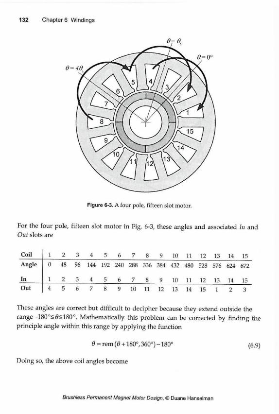
Figure 6-3. A four pole, fifteen slot motor.

For the four pole, fifteen slot motor in Fig. 6-3, these angles and associated In and Out slots are

Coil 1 2 3 4 5 6 7 8 9 10 11 12 13 14 15 Angle 0 48 96 144 192 240 288 336 384 432 480 528 576 624 672

In 1 2 3 4 5 6 7 8 9 10 11 12 13 14 15 Out 4 5 6 7 8 9 10 11 12 13 14 15 1 2 3

These angles are correct but difficult to decipher because they extend outside the range -18O°<0<18O°. Mathematically this problem can be corrected by finding the principle angle within this range by applying the function

9 = rem (6 + 180°, 360°) -180° (6.9)

Doing so, the above coil angles become

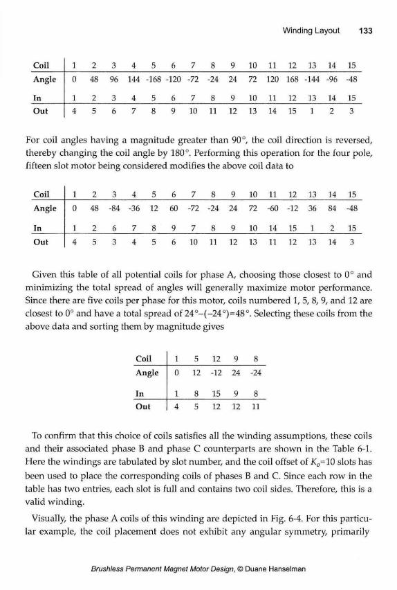
Coil 1 2 3 4 5 6 7 8 9 10 11 12 13 14 15

Angle 0 48 96 144 -168 -120 -72 -24 24 72 120 168 -144 -96 -48

In 1 2 3 4 5 6 7 8 9 10 11 12 13 14 15

Out 4 5 6 7 8 9 10 11 12 13 14 15 1 2 3

For coil angles having a magnitude greater than 90°, the coil direction is reversed, thereby changing the coil angle by 180°. Performing this operation for the four pole, fifteen slot motor being considered modifies the above coil data to

Coil 1 2 3 4 5 6 7 8 9 10 11 12 13 14 15

Angle 0 48 -84 -36 12 60 -72 -24 24 72 -60 -12 36 84 -48

In 1 2 6 7 8 9 7 8 9 10 14 15 1 2 15

Out 4 5 3 4 5 6 10 11 12 13 11 12 13 14 3

Given this table of all potential coils for phase A, choosing those closest to 0° and minimizing the total spread of angles will generally maximize motor performance. Since there are five coils per phase for this motor, coils numbered 1, 5, 8, 9, and 12 are closest to 0° and have a total spread of 24°-(-24°)=48°. Selecting these coils from the above data and sorting them by magnitude gives

Coil 1 5 12 9 8

Angle 0 12 -12 24 -24

In 1 8 15 9 8

Out 4 5 12 12 11

To confirm that this choice of coils satisfies all the winding assumptions, these coils and their associated phase B and phase C counterparts are shown in the Table 6-1. I iere the windings are tabulated by slot number, and the coil offset of K0= 10 slots has been used to place the corresponding coils of phases B and C. Since each row in the table has two entries, each slot is full and contains two coil sides. Therefore, this is a valid winding.

Visually, the phase A coils of this winding are depicted in Fig. 6-4. For this particu-lar example, the coil placement does not exhibit any angular symmetry, primarily

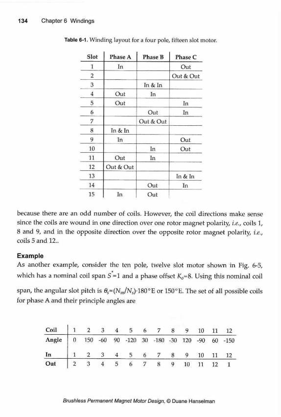
Table 6-1. Winding layout for a four pole, fifteen slot motor.

Slot Phase A Phase B Phase C

1 In Out 2 Out & Out 3 In & In 4 Out Tn

5 Out In 6 Out In 7 Out & Out

8 In & In

9 In Out 10 In Out 11 Out In 12 Out & Out

13 In & In 14 Out In

15 In Out

because there are an odd number of coils. However, the coil directions make sense since the coils are wound in one direction over one rotor magnet polarity, i.e., coils 1, 8 and 9, and in the opposite direction over the opposite rotor magnet polarity, i.e., coils 5 and 12..

Example As another example, consider the ten pole, twelve slot motor shown in Fig. 6-5,

*

which has a nominal coil span S =1 and a phase offset K0= 8. Using this nominal coil

span, the angular slot pitch is 0s=(Nm/Ns)-18O°E or 150°E. The set of all possible coils for phase A and their principle angles are

Coil 1 2 3 4 5 6 7 8 9 10 11 12

Angle 0 150 -60 90 -120 30 -180 -30 120 -90 60 -150

In 1 2 3 4 5 6 7 8 9 10 11 12 Out 2 3 4 5 6 7 8 9 10 11 12 1

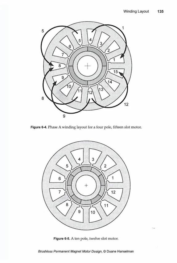
Figure 6-4. Phase A winding layout for a four pole, fifteen slot motor.

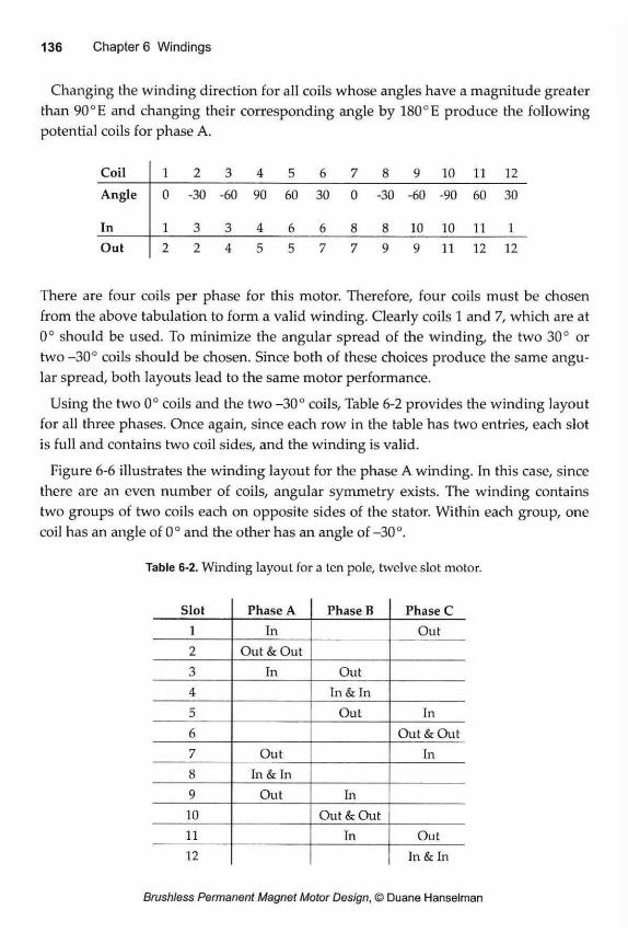
Changing the winding direction for all coils whose angles have a magnitude greater than 90°E and changing their corresponding angle by 180°E produce the following potential coils for phase A.

Coil 1 2 3 4 5 6 7 8 9 10 11 12

Angle 0 -30 -60 90 60 30 0 -30 -60 -90 60 30

In 1 3 3 4 6 6 8 8 10 10 11 1

Out 2 2 4 5 5 7 7 9 9 11 12 12

There are four coils per phase for this motor. Therefore, four coils must be chosen from the above tabulation to form a valid winding. Clearly coils 1 and 7, which are at 0° should be used. To minimize the angular spread of the winding, the two 30° or two -30° coils should be chosen. Since both of these choices produce the same angu-lar spread, both layouts lead to the same motor performance.

Using the two 0° coils and the two -30° coils, Table 6-2 provides the winding layout for all three phases. Once again, since each row in the table has two entries, each slot is full and contains two coil sides, and the winding is valid.

Figure 6-6 illustrates the winding layout for the phase A winding. In this case, since there are an even number of coils, angular symmetry exists. The winding contains two groups of two coils each on opposite sides of the stator. Within each group, one coil has an angle of 0° and the other has an angle of -30°.

Table 6-2. Winding layout for a ten pole, twelve slot motor.

Slot Phase A Phase B Phase C 1 In Out

2 Out & Out

3 In Out

4 In & In

5 Out In

6 Out & Out

7 Out In

8 In&Tn

9 Out In

10 Out & Out

11 In Out 12 In & In

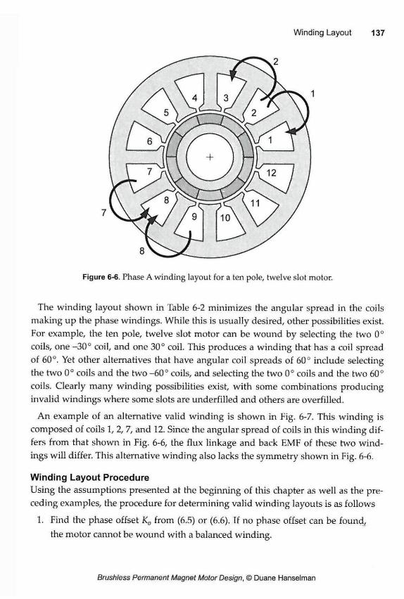
The winding layout shown in Table 6-2 minimizes the angular spread in the coils making up the phase windings. While this is usually desired, other possibilities exist. For example, the ten pole, twelve slot motor can be wound by selecting the two 0° coils, one -30° coil, and one 30° coil. This produces a winding that has a coil spread of 60°. Yet other alternatives that have angular coil spreads of 60° include selecting the two 0° coils and the two -60° coils, and selecting the two 0° coils and the two 60° coils. Clearly many winding possibilities exist, with some combinations producing invalid windings where some slots are underfilled and others are overfilled.

An example of an alternative valid winding is shown in Fig. 6-7. This winding is composed of coils 1, 2, 7, and 12. Since the angular spread of coils in this winding dif-fers from that shown in Fig. 6-6, the flux linkage and back EMF of these two wind-ings will differ. This alternative winding also lacks the symmetry shown in Fig. 6-6.

Winding Layout Procedure Using the assumptions presented at the beginning of this chapter as well as the pre-ceding examples, the procedure for determining valid winding layouts is as follows

1. Find the phase offset K0 from (6.5) or (6.6). If no phase offset can be found, the motor cannot be wound with a balanced winding.

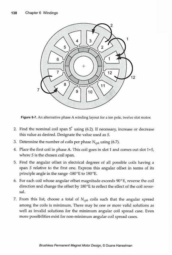
2. Find the nominal coil span S* using (6.2). If necessary, increase or decrease this value as desired. Designate the value used as S.

3. Determine the number of coils per phase N i, using (6.7).

4. Place the first coil in phase A. This coil goes in slot 1 and comes out slot 1+S, where S is the chosen coil span.

5. Find the angular offset in electrical degrees of all possible coils having a span S relative to the first one. Express this angular offset in terms of its principle angle in the range -180°E to 180°E.

6. For each coil whose angular offset magnitude exceeds 90°E, reverse the coil direction and change the offset by 180°E to reflect the effect of the coil rever-sal.

7. From this list, choose a total of NCfll, coils such that the angular spread among the coils is minimum. There may be one or more valid solutions as well as invalid solutions for the minimum angular coil spread case. Even more possibilities exist for non-minimum angular coil spread cases.

8. Using the coil offset K0, determine the winding layout for phases B and C. The phase B winding is shifted K0 slots from the phase A winding, and the phase C winding is shifted K0 slots from the phase B winding.

9. The winding is valid if all slots contain exactly two coil sides each. If the winding is not valid, other possibilities must be considered by returning to procedure step number 7.

6.5 Coil Connections

Once a winding layout has been determined, the individual coils making up each phase must be connected together in some way to form the phase winding. The sim-plest and most common approach is to connect all coils in series. When this is done, the winding can start at any slot specified by the winding layout. Similarly the phase winding can stop anywhere as well, as long as all specified turns are wound in the specified direction in specified slots.

As was illustrated in Chapter 4, individual coils can be connected in combinations of series and parallel to form phase windings. If the back EMFs of the coils connected in parallel are not identical in amplitude, shape, and angle, current circulates among the coils connected in parallel, thereby reducing motor performance. Given a specific winding layout, combinations of series and parallel that do not suffer from circulat-ing currents can be identified.

For example, consider the four pole, fifteen slot motor winding shown in Fig. 6-4. None of the coils in this winding share the same angle. Furthermore, since the num-ber of coils per phase, i.e., Ncpi,=5, is a prime number, all coils must be placed in series or all coils must be placed in parallel. No other feasible combinations exist. Because the relative angles of the coils are all different in this example, connecting all wind-ings in parallel would lead to circulating currents. That leaves connecting all coils in series as the only reasonable possibility for this pole and slot combination.

The situation is much different for the ten pole, twelve slot motor winding shown in Fig. 6-6. Here two coil groups are readily visible. In addition, Nc^i=4 is not a prime number. The coils within each group are at relative coil angles of 0° and -30° respec-tively. Therefore, if the coils within each group (i.e., one coil at 0° and one at -30°) are connected in series, and the two groups are connected in parallel, no circulating currents are created since the net back EMF is identical for each group. Adoption of this connection scheme forms two parallel paths through the winding.

By adopting the alternate winding for the ten pole, twelve slot motor shown in Fig. 6-7, no coil groups are formed. As a result, it is not possible to connect the coils in any way other than all coils in series. Any other connection creates circulating currents.

Based on these examples, the ability to connect all coils in parallel is restricted to integral slot motors where all coils have the same relative angle, such as the four pole, twelve slot motor shown in Fig. 4-12. The ability to connect coils in combina-tions of series and parallel is restricted by the primeness of Nc„h and by the number of unique coil offset angles. In cases where coil groupings can be identified, some com-binations of series and parallel are possible.

If one ignores the circulating currents produced when coils having different offset angles are connected in parallel, the prime factors of Ncph determine the valid series and parallel combinations. For example, in the four pole, fifteen slot motor, there are five coils per phase, which has one and five as its prime factors. This means that all coils can be connected in series (five) or all in parallel (one). In the four pole, twelve slot motor, there are four coils per phase. The prime factors of four are one, two, and four. Therefore, all coils can be connected in series (four), all coils can be connected in parallel (one), or two coils can be connected in series, and these two coil sets can be connected in parallel (two).

6.6 Winding Factor

In traditional motor design, pitch and distribution factors are defined that relate the back EMF of a series connection of coils to the individual coil back EMFs. The distri-bution factor takes into account the distribution of coil offset angles, and the pitch factor takes into account the effect of coil pitch. Given the back EMF of one full pitch coil, application of the pitch and distribution factors leads to the net back EMF of the phase winding. The basis for these two factors was demonstrated in Chapter 4.

In most applications of the pitch and distribution factors, the coil back EMF was assumed to be sinusoidal or the harmonics were ignored because sinusoidal currents were applied to the motor. In this situation, the pitch and distribution factors were relatively simple to compute. In addition, both factors were commonly combined and called the winding factor.

Since motor design is seldom done by hand any more, it is not necessary to derive or use either of these two factors. When using a computer, motor designers can manipulate Fourier series to describe basic waveforms. It is not necessary to limit analysis to a fundamental sinusoid when Fourier series manipulation permits consid-eration of an arbitrary number of harmonics. As a result, these conventional factors

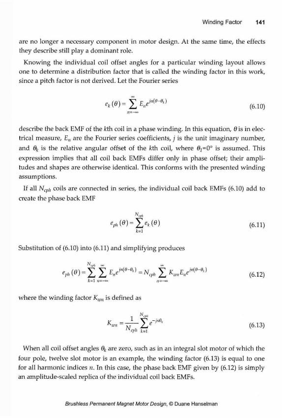
are no longer a necessary component in motor design. At the same time, the effects they describe still play a dominant role.

Knowing the individual coil offset angles for a particular winding layout allows one to determine a distribution factor that is called the winding factor in this work, since a pitch factor is not derived. Let the Fourier series

(6.10)

describe the back EMF of the A r t h coil in a phase winding. In this equation, 0 is in elec-trical measure, En are the Fourier series coefficients, j is the unit imaginary number, and OK is the relative angular offset of the fcth coil, where 0j=O° is assumed. This expression implies that all coil back EMFs differ only in phase offset; their ampli-tudes and shapes are otherwise identical. This conforms with the presented winding assumptions.

If all NCpi, coils are connected in series, the individual coil back EMFs (6.10) add to create the phase back EMF

epi,(e) = Jjek(6) ( 6 1 1 ) J t = i

Substitution of (6.10) into (6.11) and simplifying produces

k=1 h=

where the winding factor Kwn is defined as

fV 1

« - - ¡ r - Z « - * N (''") <J'>i k-1

When all coil offset angles 9k are zero, such as in an integral slot motor of which the four pole, twelve slot motor is an example, the winding factor (6.13) is equal to one for all harmonic indices n. In this case, the phase back EMF given by (6.12) is simply an amplitude-scaled replica of the individual coil back EMFs.

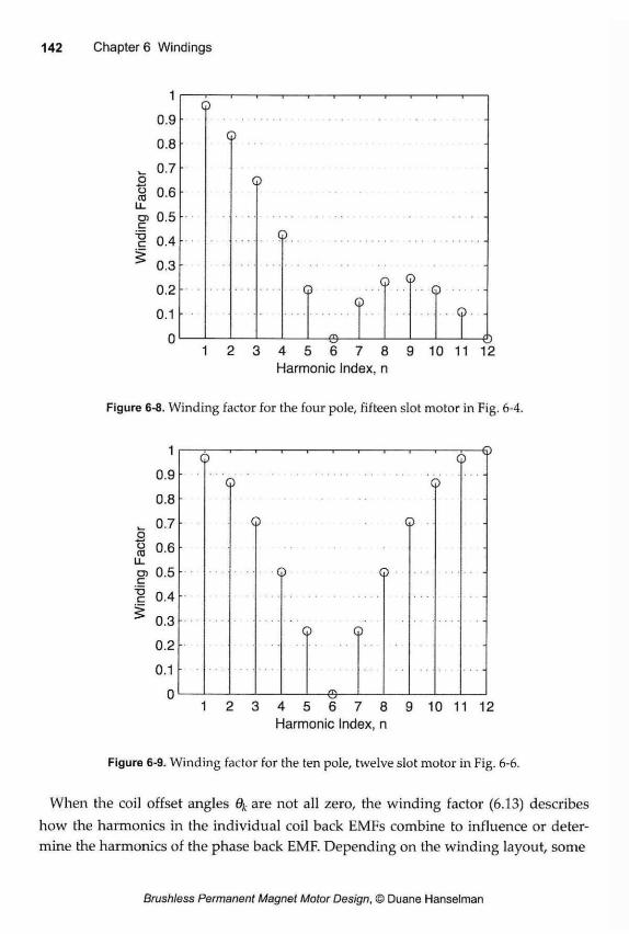
o to L i -ra c T3 c

1

0.9

0.8

0.7

0 .6

0.5

0.4

0.3

0.2

0.1

0

Q -1 1 1 1 1 1 I 1 I-

Q

Q

Q

Q

-e-

Q Q ©

©

. Q - ©

1 2 3 4 5 6 7 8 9 10 11 12 Harmonic Index, n

Figure 6-8. Winding factor for the four pole, fifteen slot motor in Fig. 6-4.

ra c TJ G

1

0.9

0.8

0.7

0.6

0.5

0.4

0.3

0.2

0.1

0

© -1 1 1 1 1 1 1 1 I—

Q

©

Q

© E—©

Q

Q

®

Q Q

1 2 3 4 5 6 7 8 9 10 11 12 Harmonic Index, n

Figure 6-9. Winding factor for the ten pole, twelve slot motor in Fig. 6-6.

When the coil offset angles 6k are not all zero, the winding factor (6.13) describes how the harmonics in the individual coil back EMFs combine to influence or deter-mine the harmonics of the phase back EMF. Depending on the winding layout, some

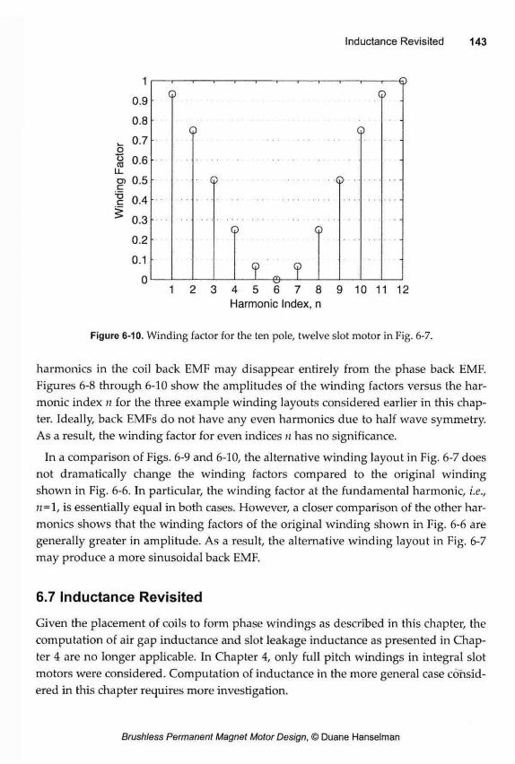
O) c TJ C

1

0.9

0 .8

0.7

0 .6

0.5

0.4

0.3

0.2

0.1

0

Q

Q

Q

? „ ?

-r © Q

Q

©

1 2 3 4 5 6 7 8 9 10 11 12 Harmonie Index, n

Figure 6-10. Winding factor for the ten pole, twelve slot motor in Fig. 6-7.

harmonics in the coil back EMF may disappear entirely from the phase back EMF. Figures 6-8 through 6-10 show the amplitudes of the winding factors versus the har-monic index n for the three example winding layouts considered earlier in this chap-ter. Ideally, back EMFs do not have any even harmonics due to half wave symmetry. As a result, the winding factor for even indices tt has no significance.

In a comparison of Figs. 6-9 and 6-10, the alternative winding layout in Fig. 6-7 does not dramatically change the winding factors compared to the original winding shown in Fig. 6-6. In particular, the winding factor at the fundamental harmonic, i.e., n=1, is essentially equal in both cases. However, a closer comparison of the other har-monics shows that the winding factors of the original winding shown in Fig. 6-6 are generally greater in amplitude. As a result, the alternative winding layout in Fig. 6-7 may produce a more sinusoidal back EMF.

6.7 Inductance Revisited

Given the placement of coils to form phase windings as described in this chapter, the computation of air gap inductance and slot leakage inductance as presented in Chap-ter 4 are no longer applicable. In Chapter 4, only full pitch windings in integral slot motors were considered. Computation of inductance in the more general case consid-ered in this chapter requires more investigation.

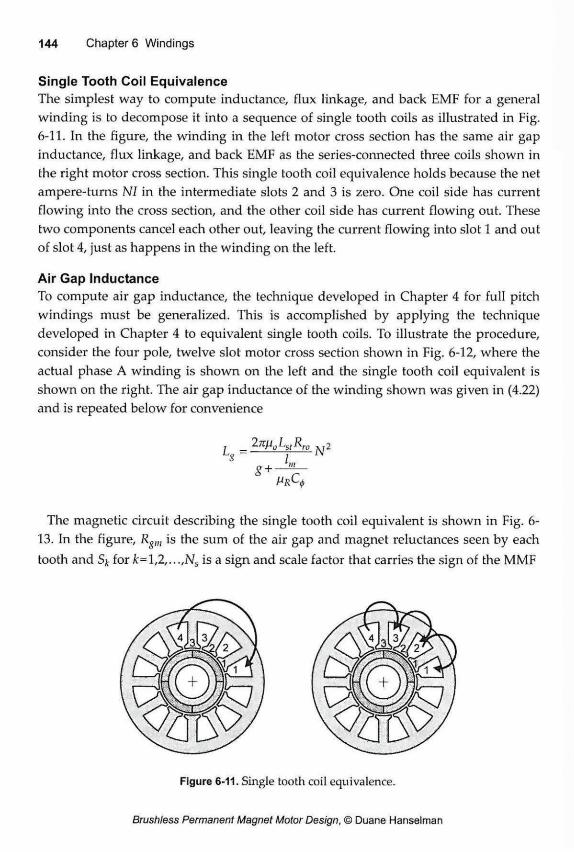
Single Tooth Coil Equivalence The simplest way to compute inductance, flux linkage, and back EMF for a general winding is to decompose it into a sequence of single tooth coils as illustrated in Fig. 6-11. In the figure, the winding in the left motor cross section has the same air gap inductance, flux linkage, and back EMF as the series-connected three coils shown in the right motor cross section. This single tooth coil equivalence holds because the net ampere-turns NI in the intermediate slots 2 and 3 is zero. One coil side has current flowing into the cross section, and the other coil side has current flowing out. These two components cancel each other out, leaving the current flowing into slot 1 and out of slot 4, just as happens in the winding on the left.

Air Gap Inductance To compute air gap inductance, the technique developed in Chapter 4 for full pitch windings must be generalized. This is accomplished by applying the technique developed in Chapter 4 to equivalent single tooth coils. To illustrate the procedure, consider the four pole, twelve slot motor cross section shown in Fig. 6-12, where the actual phase A winding is shown on the left and the single tooth coil equivalent is shown on the right. The air gap inductance of the winding shown was given in (4.22) and is repeated below for convenience

r _ 2np0LstRro 2 $ I

g + - J m -VrCJ,

The magnetic circuit describing the single tooth coil equivalent is shown in Fig. 6-13. In the figure, Rgm is the sum of the air gap and magnet reluctances seen by each tooth and Sk for k=l,2,...,Ns is a sign and scale factor that carries the sign of the MMF

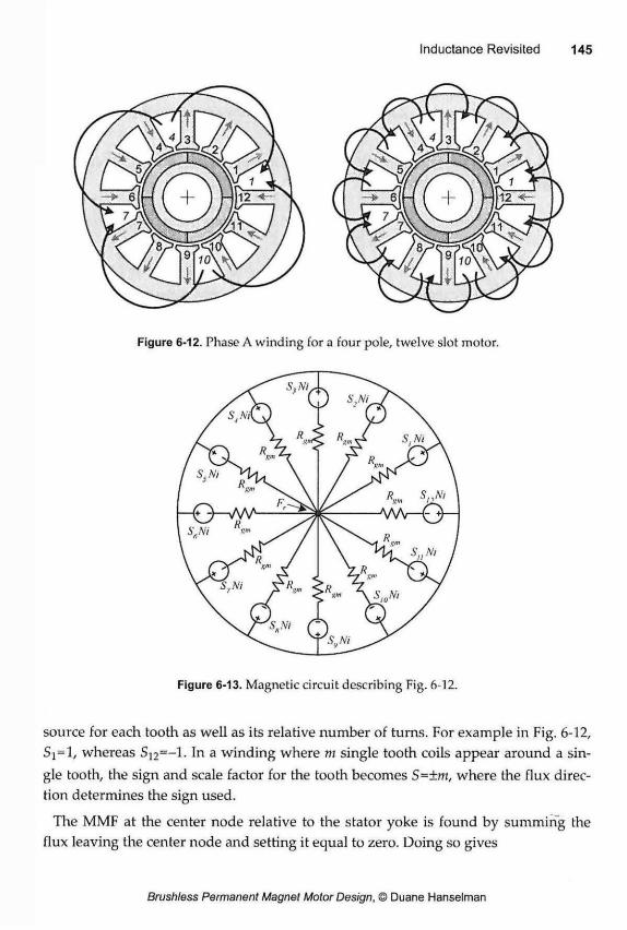
Figure 6-12. Phase A winding for a four pole, twelve slot motor.

source for each tooth as well as its relative number of turns. For example in Fig. 6-12, Si=l, whereas S ] 2 = - l . In a winding where m single tooth coils appear around a sin-gle tooth, the sign and scale factor for the tooth becomes S=±m, where the flux direc-tion determines the sign used.

The MMF at the center node relative to the stator yoke is found by summing the flux leaving the center node and setting it equal to zero. Doing so gives

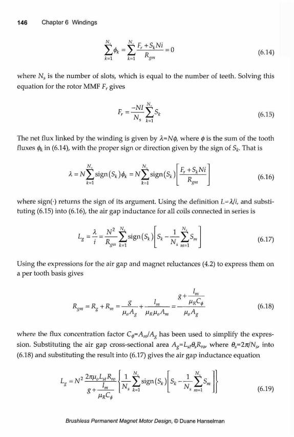
Jt=l k=1 S"' (6.14)

where Ns is the number of slots, which is equal to the number of teeth. Solving this equation for the rotor MMF Fr gives

Fr = -MI N S Jt=l

(6.15)

The net flux linked by the winding is given by A=N0, where 0 is the sum of the tooth fluxes in (6.14), with the proper sign or direction given by the sign of Sk. That is

A = N ^ s i g n ( S t ) 4 = N ^ s i g n ( S i ) Jr=l k=1

Fr+SkNi R gm

(6.16)

where sign(-) returns the sign of its argument. Using the definition L=A/i, and substi-tuting (6.15) into (6.16), the air gap inductance for all coils connected in series is

A N 2 N,

i R - È s i g n ( S , )

V" k=1

N.

N. S m=l (6.17)

Using the expressions for the air gap and magnet reluctances (4.2) to express them on a per tooth basis gives

Rgm = + R„ 8 I 8 +

L

(6.18)

where the flux concentration factor C^AJA^ has been used to simplify the expres-sion. Substituting the air gap cross-sectional area Ag=LsiGsRro, where 0s=2n/Ns, into (6.18) and substituting the result into (6.17) gives the air gap inductance equation

LS=N 2 2 y i 0 L s t R r c I 1

8 + MrC

— £ s i g n ( S , ) S Jt=l

s * - — y s „ k N ¿s * s m=l (6.19)

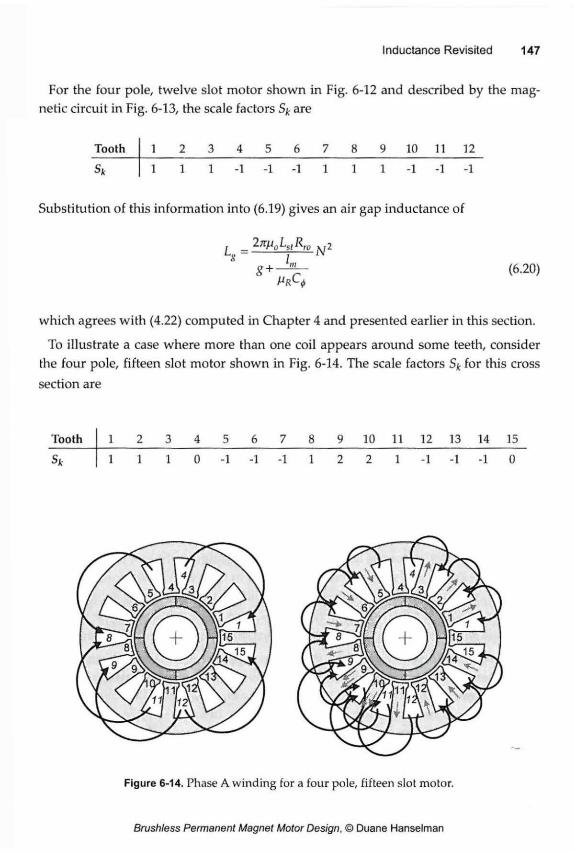
For the four pole, twelve slot motor shown in Fig. 6-12 and described by the mag-netic circuit in Fig. 6-13, the scale factors Sk are

Tooth 1 2 3 4 5 6 7 8 9 10 11 12

s k 1 1 1 -1 -1 -1 1 1 1 -1 -1 -1

Substitution of this information into (6.19) gives an air gap inductance of

, _ 2^ 0 L s > K r o 2 ~ / ™

g + (6.20)

which agrees with (4.22) computed in Chapter 4 and presented earlier in this section.

To illustrate a case where more than one coil appears around some teeth, consider the four pole, fifteen slot motor shown in Fig. 6-14. The scale factors Stt for this cross section are

Tooth 1 2 3 4 5 6 7 8 9 10 11 12 13 14 15

sk 1 1 1 0 -1 -1 -1 1 2 2 1 -1 -1 -1 0

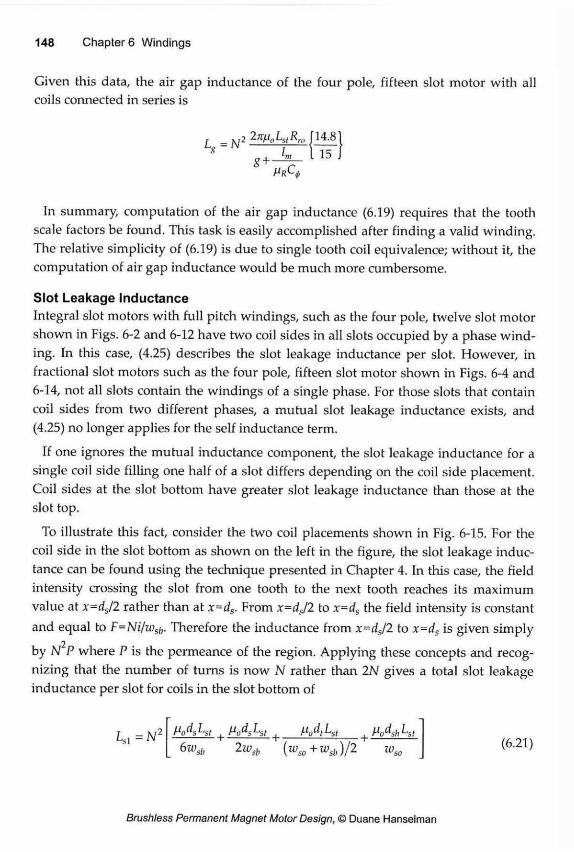
Given this data, the air gap inductance of the four pole, fifteen slot motor with all coils connected in series is

In summary, computation of the air gap inductance (6.19) requires that the tooth scale factors be found. This task is easily accomplished after finding a valid winding. The relative simplicity of (6.19) is due to single tooth coil equivalence; without it, the computation of air gap inductance would be much more cumbersome.

Slot Leakage Inductance Integral slot motors with full pitch windings, such as the four pole, twelve slot motor shown in Figs. 6-2 and 6-12 have two coil sides in all slots occupied by a phase wind-ing. In this case, (4.25) describes the slot leakage inductance per slot. However, in fractional slot motors such as the four pole, fifteen slot motor shown in Figs. 6-4 and 6-14, not all slots contain the windings of a single phase. For those slots that contain coil sides from two different phases, a mutual slot leakage inductance exists, and (4.25) no longer applies for the self inductance term.

If one ignores the mutual inductance component, the slot leakage inductance for a single coil side filling one half of a slot differs depending on the coil side placement. Coil sides at the slot bottom have greater slot leakage inductance than those at the slot top.

To illustrate this fact, consider the two coil placements shown in Fig. 6-15. For the coil side in the slot bottom as shown on the left in the figure, the slot leakage induc-tance can be found using the technique presented in Chapter 4. In this case, the field intensity crossing the slot from one tooth to the next tooth reaches its maximum value at x=dj2 rather than at x=ds. From x=dj2 to x=ds the field intensity is constant and equal to F=Ni/iosb. Therefore the inductance from x-dJ2 to x=ds is given simply

by N P where P is the permeance of the region. Applying these concepts and recog-nizing that the number of turns is now N rather than 2N gives a total slot leakage inductance per slot for coils in the slot bottom of

•2 2nf.i0LstR,0

2 MpdJ-s, | n A h t , M Lst t Updsh t _ 6wsb 2wsb (wso+wsh )/2 ioS0 'si,

+ lo"tust (6.21)

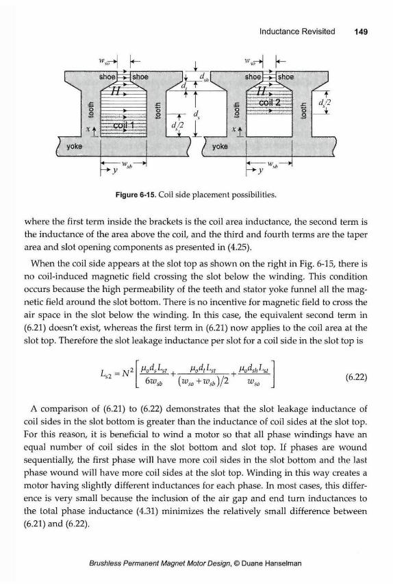
w H h i i rH h

Figure 6-15. Coil side placement possibilities.

where the first term inside the brackets is the coil area inductance, the second term is the inductance of the area above the coil, and the third and fourth terms are the taper area and slot opening components as presented in (4.25).

When the coil side appears at the slot top as shown on the right in Fig. 6-15, there is no coil-induced magnetic field crossing the slot below the winding. This condition occurs because the high permeability of the teeth and stator yoke funnel all the mag-netic field around the slot bottom. There is no incentive for magnetic field to cross the air space in the slot below the winding. In this case, the equivalent second term in (6.21) doesn't exist, whereas the first term in (6.21) now applies to the coil area at the slot top. Therefore the slot leakage inductance per slot for a coil side in the slot top is

6wsb (wso+wsb)/2 wso J <6-22)

A comparison of (6.21) to (6.22) demonstrates that the slot leakage inductance of coil sides in the slot bottom is greater than the inductance of coil sides at the slot top. For this reason, it is beneficial to wind a motor so that all phase windings have an equal number of coil sides in the slot bottom and slot top. If phases are wound sequentially, the first phase will have more coil sides in the slot bottom and the last phase wound will have more coil sides at the slot top. Winding in this way creates a motor having slightly different inductances for each phase. In most cases, this differ-ence is very small because the inclusion of the air gap and end turn inductances to the total phase inductance (4.31) minimizes the relatively small difference between (6.21) and (6.22).

Given the inductance expressions provided here as well as those given in Chapter 4, the phase inductance of any general winding is easily computed by careful appli-cation of the expressions for the air gap, slot leakage, and end turn inductances.

6.8 Summary

This chapter considered fundamental concepts and criteria for winding a brushless permanent magnet motor. Concepts such as coil span, phase offset, and winding fac-tor were presented. Criteria were presented to identify valid pole and slot counts that support a balanced winding. Based on examples, a procedure was presented for winding any general motor that can support a balanced winding. To compute the inductance of windings other than the full pitch windings considered in Chapter 4, the concept of single tooth coil equivalence was introduced and used to generalize expressions for air gap inductance. Finally, slot leakage inductance was generalized to consider coils that occupy only the slot bottom or slot top.

The magnetic field distribution within a motor plays a fundamental role in motor performance. In particular, the magnetic field in the air gap and how it links to the stator coils determines the back EMF and torque. Secondarily, the magnetic field act-ing within the ferromagnetic portions of the motor determines the amplitude of the air gap flux density. If too much flux is forced through the ferromagnetic portions, they saturate and diminish the flux flow across the air gap.

While a magnetic field cannot be seen with the eyes, magnetic flux is a fluid that flows under the influence of pressure in the form of MMF. As such, the magnetic field distribution in a motor can be visualized as fluid flow that is governed by fluid dynamic principles. Within materials, including air, flux density and field intensity are vector quantities that are governed by partial differential equations.

Because of the complexity inherent in describing vector quantities in a three dimen-sional space, assumptions are commonly made to simplify the problem so that sim-ple analytical results can be obtained. This was done in Chapter 4, where magnetic field distributions were considered uniform over cross-sectional areas and the direc-tion of flux flow was assumed. These assumptions led to magnetic circuit analysis.

Magnetic circuit analysis provides rough estimates of the magnetic field distribu-tion within a motor. These estimates provide valuable insight into the fundamentals of motor operation and help identify critical parameters. Because of the inherent non-uniformity of the magnetic field distribution in the air gap, magnetic circuit analysis fails to provide accurate predictions for the flux linkage and back EMF in a brushless permanent magnet motor. For this reason, the air gap flux density distribution must be determined more accurately

This chapter covers motor design details that are associated with the magnetic field distribution in a motor. Accurate prediction of the flux density distribution within the air gap is the key issue. Given this distribution, the magnetic field distribution in the rest of the motor can be easily approximated with sufficient accuracy using mag-netic circuit analysis.

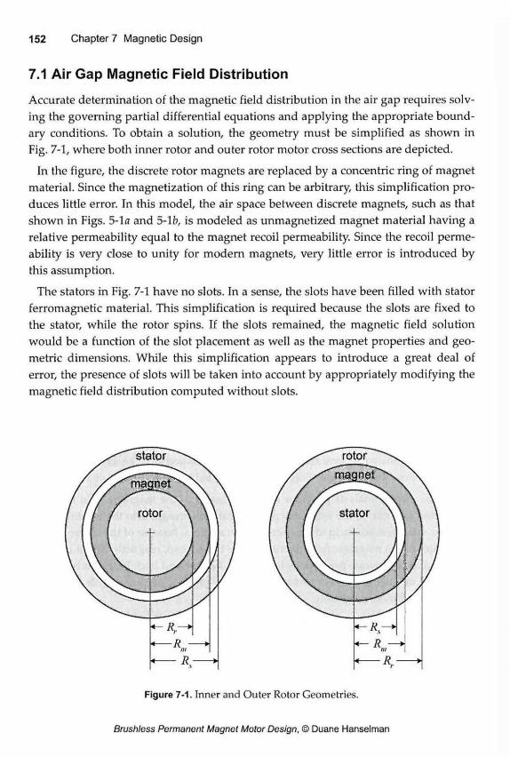
7.1 Air Gap Magnetic Field Distribution

Accurate determination of the magnetic field distribution in the air gap requires solv-ing the governing partial differential equations and applying the appropriate bound-ary conditions. To obtain a solution, the geometry must be simplified as shown in Fig. 7-1, where both inner rotor and outer rotor motor cross sections are depicted.

In the figure, the discrete rotor magnets are replaced by a concentric ring of magnet material. Since the magnetization of this ring can be arbitrary, this simplification pro-duces little error. In this model, the air space between discrete magnets, such as that shown in Figs. 5-1« and 5-1 b, is modeled as unmagnetized magnet material having a relative permeability equal to the magnet recoil permeability. Since the recoil perme-ability is very close to unity for modem magnets, very little error is introduced by this assumption.

The stators in Fig. 7-1 have no slots. In a sense, the slots have been filled with stator ferromagnetic material. This simplification is required because the slots are fixed to the stator, while the rotor spins. If the slots remained, the magnetic field solution would be a function of the slot placement as well as the magnet properties and geo-metric dimensions. While this simplification appears to introduce a great deal of error, the presence of slots will be taken into account by appropriately modifying the magnetic field distribution computed without slots.

m < R •

m R. r

Figure 7-1. Inner and Outer Rotor Geometries.

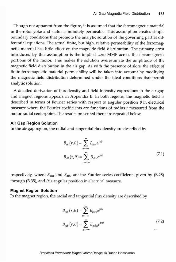
Though not apparent from the figure, it is assumed that the ferromagnetic material in the rotor yoke and stator is infinitely permeable. This assumption creates simple boundary conditions that promote the analytic solution of the governing partial dif-ferential equations. The actual finite, but high, relative permeability of the ferromag-netic material has little effect on the magnetic field distribution. The primary error introduced by this assumption is the implied zero MMF across the ferromagnetic portions of the motor. This makes the solution overestimate the amplitude of the magnetic field distribution in the air gap. As with the presence of slots, the effect of finite ferromagnetic material permeability will be taken into account by modifying the magnetic field distribution determined under the ideal conditions that permit analytic solution.

A detailed derivation of flux density and field intensity expressions in the air gap and magnet regions appears in Appendix B. In both regions, the magnetic field is described in terms of Fourier series with respect to angular position 0 in electrical measure where the Fourier coefficients are functions of radius r measured from the motor radial centerpoint. The results presented there are repeated below.

Air Gap Region Solution In the air gap region, the radial and tangential flux density are described by

Bttr(r,0) = jr Biiry° )J = -oo

respectively, where Bnrn and Bndn are the Fourier series coefficients given by (B.28) through (B.35), and 0 \s angular position in electrical measure.

Magnet Region Solution In the magnet region, the radial and tangential flux density are described by

|!=-oo

Bmd(r,e)=f^Bmene'"d ( Z 2 )

where Bmrn and Bmgn are the Fourier coefficients given by (B.37) through (B.43), and 6 is angular position in electrical measure.

Symmetry In both the air gap and magnet regions, the magnetic field exhibits halfwave symme-try for all common magnetization profiles. As a result, all even harmonics in (7.1) and (7.2) are zero. In addition, given the common magnetization profiles defined in Appendix B, the resulting radial flux density exhibits even symmetry, making all of its Fourier series coefficients real. Similarly, the resulting tangential flux density exhibits odd symmetry, making all of its Fourier series coefficients imaginary.

7.2 Influence of Stator Slots

The preceding descriptions for the magnetic field in the air gap and magnet regions apply to the slotless case where the stator surface at the air gap is infinitely perme-able. The presence of slots changes or perturbs the magnetic field throughout the air gap and magnet regions, with the perturbation varying as a function of radius or dis-tance from the slots. At the magnet and rotor yoke interface at Rr, the magnetic field experiences little perturbation, whereas the greatest perturbation occurs at the stator surface at Rs.

In addition to the magnetic field perturbation being a function of distance from the slots, it is also a function of the saturation of the ferromagnetic materials used in the rotor and stator. In particular, the saturation of the shoe tips influences the amplitude and distribution of the perturbation. Since this effect is impossible to describe ana-lytically, it must be ignored. However, it does point to the desirability of making the shoe radial depth sufficiently large to minimize shoe tip saturation. This fact calls for a compromise, since it is in conflict with maximizing the slot area available for wind-ings.

A number of techniques for describing the magnetic field perturbation due to stator slots appear in the literature. Some parameterize the perturbation throughout the air gap and magnet regions. Some accommodate shoe tip saturation by making the per-turbation apply to an empirically-determined area wider than the slot opening. In brushless permanent magnet motor design, the radial magnetic field entering the sta-tor determines the flux linkage and back EMF. As a result, the influence of stator slots need only be considered at the stator surface.

The fundamental principle governing the influence of the stator slots is the fact that the magnetic field over the slots must travel further to reach the stator ferromagnetic

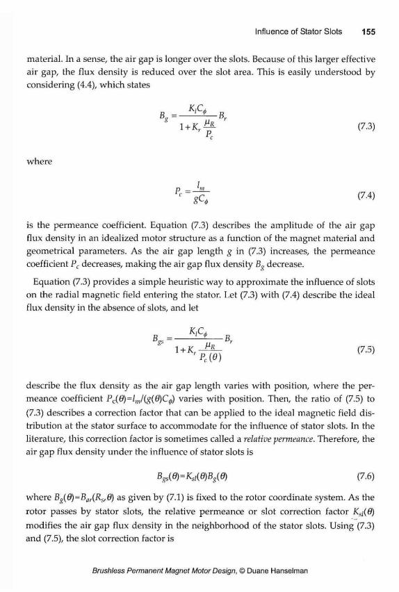
material. In a sense, the air gap is longer over the slots. Because of this larger effective air gap, the flux density is reduced over the slot area. This is easily understood by considering (4.4), which states

B„—K,C° » \+Kr — (7.3)

Pc

where

P — - " g c 4 m

is the permeance coefficient. Equation (7.3) describes the amplitude of the air gap flux density in an idealized motor structure as a function of the magnet material and geometrical parameters. As the air gap length g in (7.3) increases, the permeance coefficient PC decreases, making the air gap flux density B,, decrease.

Equation (7.3) provides a simple heuristic way to approximate the influence of slots on the radial magnetic field entering the stator. Let (7.3) with (7.4) describe the ideal flux density in the absence of slots, and let

BSs=-1 + Kr

MR

Pc (0) (7.5)

describe the flux density as the air gap length varies with position, where the per-meance coefficient Pc(9)=lm/(g(9)Cvaries with position. Then, the ratio of (7.5) to (7.3) describes a correction factor that can be applied to the ideal magnetic field dis-tribution at the stator surface to accommodate for the influence of stator slots. In the literature, this correction factor is sometimes called a relative permeance. Therefore, the air gap flux density under the influence of stator slots is

B^6)=Ksl(d)Bs(e) (7.6)

where B^(6)=Btn(Rs,6) as given by (7.1) is fixed to the rotor coordinate system. As the rotor passes by stator slots, the relative permeance or slot correction factor Ksj(d) modifies the air gap flux density in the neighborhood of the stator slots. Using (7.3) and (7.5), the slot correction factor is

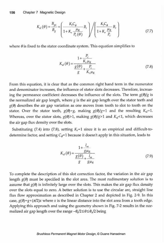
V c J

^ Br 1 + fC — f

Pr (7.7)

where 0 is fixed to the stator coordinate system. This equation simplifies to

(7.8)

From this equation, it is clear that as the common right hand term in the numerator and denominator increases, the influence of stator slots decreases. Therefore, increas-ing the permeance coefficient decreases the influence of the slots. The term g(9)/g is the normalized air gap length, where g is the air gap length over the stator teeth and g(6) describes the air gap variation as one moves from tooth to slot to tooth on the stator. Over the stator teeth, g(d)=g, making g{0)/g=1 and the resulting Ksj=1. Whereas, over the stator slots, g(0)> 1, making g(0)/g> 1 and Ksj< 1, which decreases the air gap flux density over the slots.

Substituting (7.4) into (7.8), setting Kr= 1 since it is an empirical and difficult-to-determine factor, and setting C^-l because it doesn't apply in this situation, leads to

To complete the description of this slot correction factor, the variation in the air gap length g(6) must be specified in the slot area. The most rudimentary solution is to assume that g(6) is infinitely large over the slots. This makes the air gap flux density over the slots equal to zero. A better solution is to use the circular arc, straight line flux flow approximation as described in Chapter 2 and depicted in Fig. 2-9. In this case, g(9)=g+{n/2)x where x is the linear distance into the slot area from a tooth edge. Applying this approach and using the geometry shown in Fig. 7-2 results in the nor-malized air gap length over the range -6s/2<6<ds/2 being

(7.9)

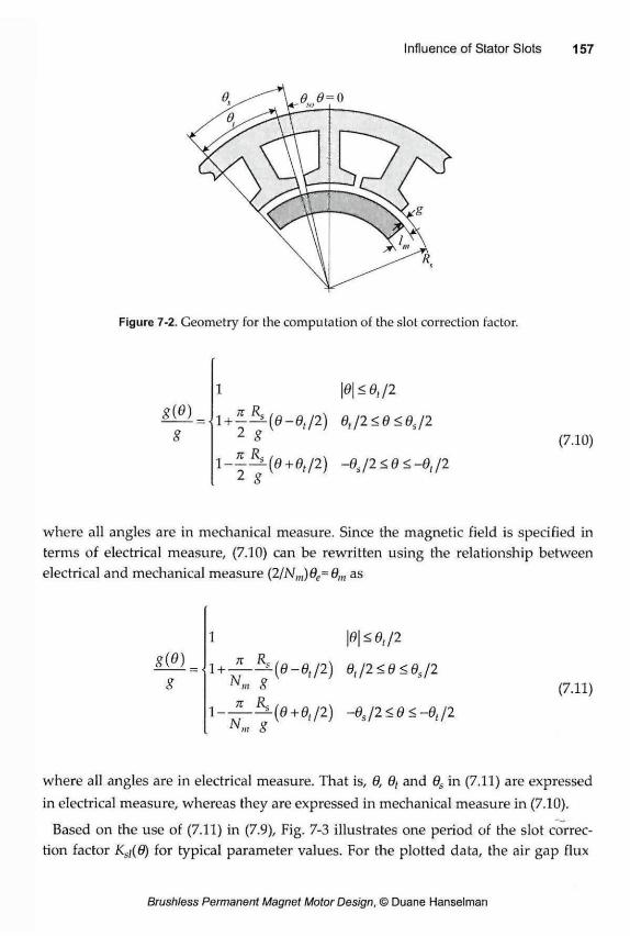
Figure 7-2. Geometry for the computation of the slot correction factor.

S(0) 1 \e\<et/2

l + | i ( 0 - 0 f / 2 ) 0 (/2<0<0 s/2

l _ | ^ ( 0 + 0 f / 2 ) -0 s /2<0 <-0 (/2 (7.10)

where all angles are in mechanical measure. Since the magnetic field is specified in terms of electrical measure, (7.10) can be rewritten using the relationship between electrical and mechanical measure (2/Nm)6e=0m as

8(0) 1 |0|<0,/2

l + J L i ( 0 _ 0 ( / 2 ) 0,/2<0<0s/2

(e + 0,/2) -0s/2<0<-0(/2 (7.11)

where all angles are in electrical measure. That is, 0, 0, and 0S in (7.11) are expressed in electrical measure, whereas they are expressed in mechanical measure in (7.10).

Based on the use of (7.11) in (7.9), Fig. 7-3 illustrates one period of the slot correc-tion factor Ksi(6) for typical parameter values. For the plotted data, the air gap flux

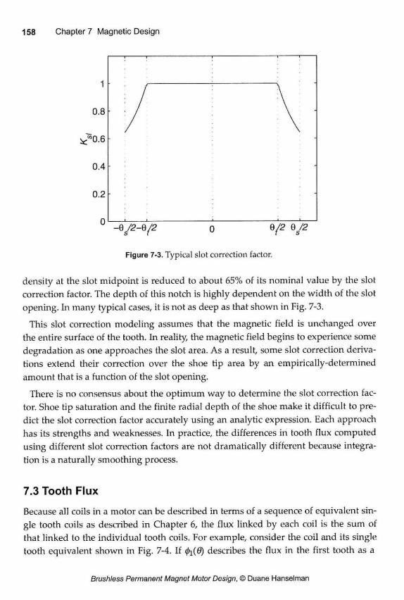
1

0.8

v^O.6

0.4

0.2

0 -e /2-Q/2 d/2 6/2 0

Figure 7-3. Typical slot correction factor.

density at the slot midpoint is reduced to about 65% of its nominal value by the slot correction factor. The depth of this notch is highly dependent on the width of the slot opening. In many typical cases, it is not as deep as that shown in Fig. 7-3.

This slot correction modeling assumes that the magnetic field is unchanged over the entire surface of the tooth. In reality, the magnetic field begins to experience some degradation as one approaches the slot area. As a result, some slot correction deriva-tions extend their correction over the shoe tip area by an empirically-determined amount that is a function of the slot opening.

There is no consensus about the optimum way to determine the slot correction fac-tor. Shoe tip saturation and the finite radial depth of the shoe make it difficult to pre-dict the slot correction factor accurately using an analytic expression. Each approach has its strengths and weaknesses. In practice, the differences in tooth flux computed using different slot correction factors are not dramatically different because integra-tion is a naturally smoothing process.

Because all coils in a motor can be described in terms of a sequence of equivalent sin-gle tooth coils as described in Chapter 6, the flux linked by each coil is the sum of that linked to the individual tooth coils. For example, consider the coil and its single tooth equivalent shown in Fig. 7-4. If <p\(6) describes the flux in the first tooth as a

7.3 Tooth Flux

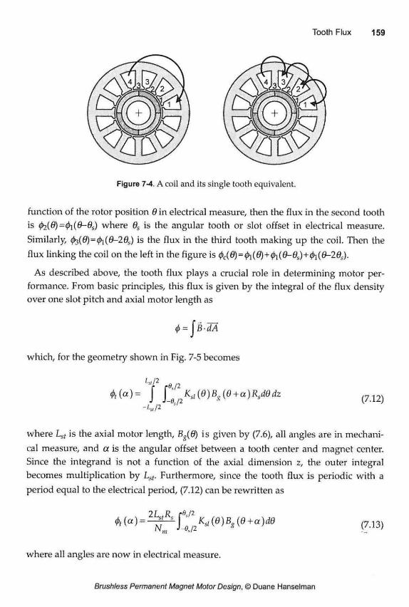
Figure 7-4. A coil and its single tooth equivalent.

function of the rotor position 6>in electrical measure, then the flux in the second tooth is <fo.(6)=<h(&-9s) where 9S is the angular tooth or slot offset in electrical measure. Similarly, =<fo(0-2ds) is the flux in the third tooth making up the coil. Then the flux linking the coil on the left in the figure is 0c(0) = <fr(0)+01(0-0s)+01(0-2&;).

As described above, the tooth flux plays a crucial role in determining motor per-formance. From basic principles, this flux is given by the integral of the flux density over one slot pitch and axial motor length as

<p = Jfi-dX

which, for the geometry shown in Fig. 7-5 becomes

i-si/2 , A(«) = J ¡'^ Ksl (6)Bx(9 +a)Rsdddz ( 7 1 2 )

where Lst is the axial motor length, B,{(6) is given by (7.6), all angles are in mechani-cal measure, and a is the angular offset between a tooth center and magnet center. Since the integrand is not a function of the axial dimension z, the outer integral becomes multiplication by Lst. Furthermore, since the tooth flux is periodic with a period equal to the electrical period, (7.12) can be rewritten as

<t,t(a) = \8^2Ksl(0)Bg(e + a)de ( 7 . 1 3 )

where all angles are now in electrical measure.

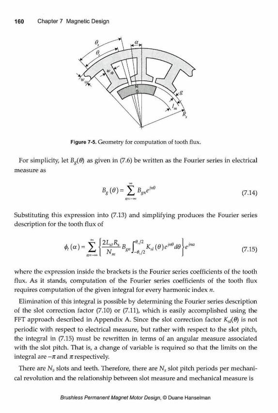
Figure 7-5. Geometry for computation of tooth flux.

For simplicity, let Bs(8) as given in (7.6) be written as the Fourier series in electrical measure as

Substituting this expression into (7.13) and simplifying produces the Fourier series description for the tooth flux of

where the expression inside the brackets is the Fourier series coefficients of the tooth flux. As it stands, computation of the Fourier series coefficients of the tooth flux requires computation of the given integral for every harmonic index n.

Elimination of this integral is possible by determining the Fourier series description of the slot correction factor (7.10) or (7.11), which is easily accomplished using the FFT approach described in Appendix A. Since the slot correction factor Ksi(6) is not periodic with respect to electrical measure, but rather with respect to the slot pitch, the integral in (7.15) must be rewritten in terms of an angular measure associated with the slot pitch. That is, a change of variable is required so that the limits on the integral are —n and TT respectively.

There are Ns slots and teeth. Therefore, there are Ns slot pitch periods per mechani-cal revolution and the relationship between slot measure and mechanical measure is

W = I V " ' ° (7.14)

(7.15)

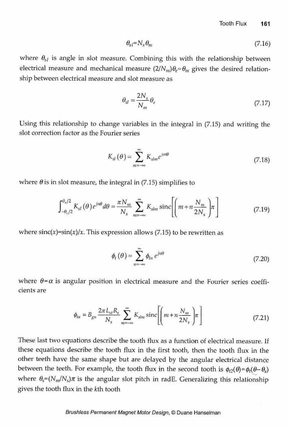
0 S ; -N s 0 m (7.16)

where GsI is angle in slot measure. Combining this with the relationship between electrical measure and mechanical measure (2/Nm)8e=9m gives the desired relation-ship between electrical measure and slot measure as

0s t = 2N, N„,

9., (7.17)

Using this relationship to change variables in the integral in (7.15) and writing the slot correction factor as the Fourier series

Ks,(0)= E V e (7.18)

where 0is in slot measure, the integral in (7.15) simplifies to

xN,. N,

m + n—— \n 2 N« (7.19)

where sinc(x)=sin(x)/x. This expression allows (7.15) to be rewritten as

juö (7.20)

where 9= a is angular position in electrical measure and the Fourier series coeffi-cients are

rtn - "g„ o 2nLstR y

sine m + n-2NC (7.21)

These last two equations describe the tooth flux as a function of electrical measure. If these equations describe the tooth flux in the first tooth, then the tooth flux in the other teeth have the same shape but are delayed by the angular electrical distance between the teeth. For example, the tooth flux in the second tooth is 0,2(0)=0f(0-0s) where 9s=(Nm/Ns)7t is the angular slot pitch in radE. Generalizing this relationship gives the tooth flux in the kth tooth

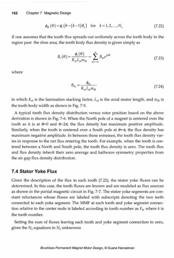
h(0) = <f>,{0-(k-m) for A = 1,2. N s (7.22)

If one assumes that the tooth flux spreads out uniformly across the tooth body in the region past the shoe area, the tooth body flux density is given simply as

where

R - h» ~ K I w (7'24)

si st tb

in which Ks/ is the lamination stacking factor, Lst is the axial motor length, and z% is the tooth body width as shown in Fig. 7-5.

A typical tooth flux density distribution versus rotor position based on the above derivation is shown in Fig. 7-6. When the North pole of a magnet is centered over the tooth as it is at 0=0 and 6=2k, the flux density has maximum positive amplitude. Similarly, when the tooth is centered over a South pole at 6=n, the flux density has maximum negative amplitude. In between these extremes, the tooth flux density var-ies in response to the net flux entering the tooth. For example, when the tooth is cen-tered between a North and South pole, the tooth flux density is zero. The tooth flux and flux density inherit their zero average and halfwave symmetry properties from the air gap flux density distribution.

7.4 Stator Yoke Flux

Given the description of the flux in each tooth (7.22), the stator yoke fluxes can be determined. In this case, the tooth fluxes are known and are modeled as flux sources as shown in the partial magnetic circuit in Fig. 7-7. The stator yoke segments are con-stant reluctances whose fluxes are labeled with subscripts denoting the two teeth connected to each yoke segment. The MMF at each tooth and yoke segment connec-tion relative to the center node is labeled according to tooth number as Fjt, where k is the tooth number.

Setting the sum of fluxes leaving each tooth and yoke segment connection to zero, gives the Ns equations in Ns unknowns

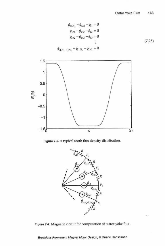
<Ps IN, -&21-0H = 0

&21 ~0s32 -<t>t2 = 0

&32 ~&43 -<t>t3 = 0

: (7.25)

Figure 7-6. A typical tooth flux density distribution.

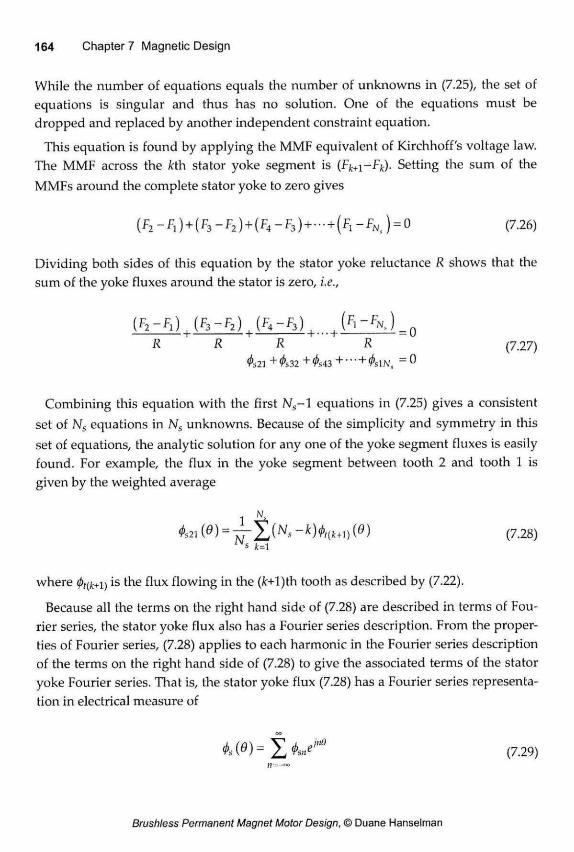
While the number of equations equals the number of unknowns in (7.25), the set of equations is singular and thus has no solution. One of the equations must be dropped and replaced by another independent constraint equation.

This equation is found by applying the MMF equivalent of Kirchhoff's voltage law. The MMF across the kth stator yoke segment is (Fk+l-Fk). Setting the sum of the MMFs around the complete stator yoke to zero gives

( F 2 - f 1 ) + ( F 3 - F 2 ) + ( F 4 - F 3 ) + - + ( F 1 - F N s ) = 0 (7.26)

Dividing both sides of this equation by the stator yoke reluctance R shows that the sum of the yoke fluxes around the stator is zero, i.e.,

( F 2 - f i ) | ( f 3 - F 2 ) | ( f 4 - F 3 ) | , ( F i - * x ) _ 0

R R R R (727) &21 + & 32 +&43 + + = 0

Combining this equation with the first Ns~ 1 equations in (7.25) gives a consistent set of Ns equations in Ns unknowns. Because of the simplicity and symmetry in this set of equations, the analytic solution for any one of the yoke segment fluxes is easily found. For example, the flux in the yoke segment between tooth 2 and tooth 1 is given by the weighted average

1 N '

&21 (0) = T r X ( w S - * M ( W ) ( 0 ) (7.28) S Jt=l

where <¡>¡ +1) i s ^e flux flowing in the (/r+l)th tooth as described by (7.22).

Because all the terms on the right hand side of (7.28) are described in terms of Fou-rier series, the stator yoke flux also has a Fourier series description. From the proper-ties of Fourier series, (7.28) applies to each harmonic in the Fourier series description of the terms on the right hand side of (7.28) to give the associated terms of the stator yoke Fourier series. That is, the stator yoke flux (7.28) has a Fourier series representa-tion in electrical measure of

| > s „ e ' " S (7-29)

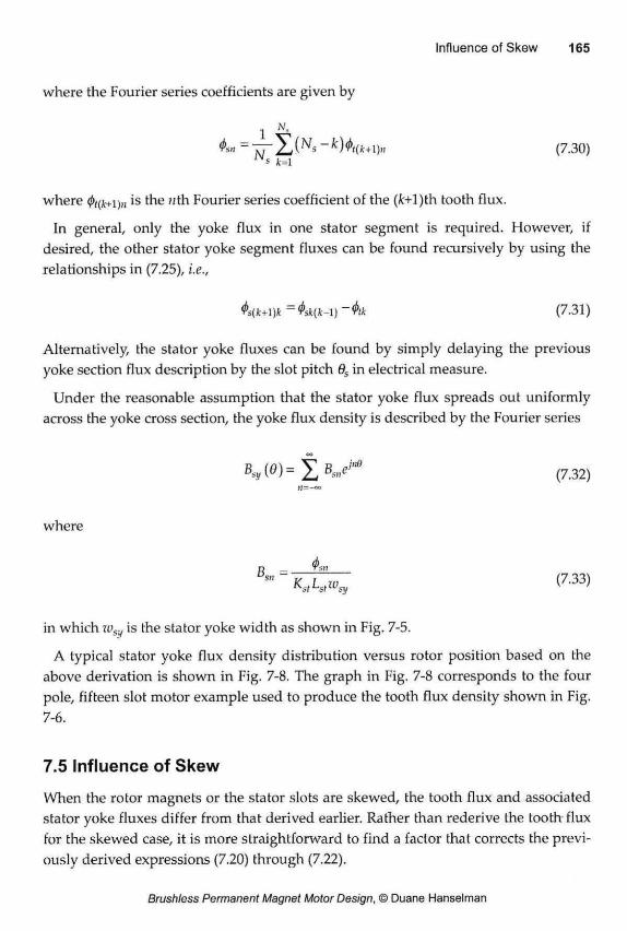
where the Fourier series coefficients are given by

1 X -k)<t>t(M)„ (7.30)

where (j> k+i)n the »th Fourier series coefficient of the (Ar+1 )th tooth flux.

In general, only the yoke flux in one stator segment is required. However, if desired, the other stator yoke segment fluxes can be found recursively by using the relationships in (7.25), i.e.,

(7.31)

Alternatively, the stator yoke fluxes can be found by simply delaying the previous yoke section flux description by the slot pitch 9S in electrical measure.

Under the reasonable assumption that the stator yoke flux spreads out uniformly across the yoke cross section, the yoke flux density is described by the Fourier series

CO B s y(d)= X ^ (7.32)

M=—00

where

M B~„ -S" ~ KstLslwsy (7-33)

in which wsy is the stator yoke width as shown in Fig. 7-5.

A typical stator yoke flux density distribution versus rotor position based on the above derivation is shown in Fig. 7-8. The graph in Fig. 7-8 corresponds to the four pole, fifteen slot motor example used to produce the tooth flux density shown in Fig. 7-6.

7.5 Influence of Skew

When the rotor magnets or the stator slots are skewed, the tooth flux and associated stator yoke fluxes differ from that derived earlier. Rather than rederive the tooth flux for the skewed case, it is more straightforward to find a factor that corrects the previ-ously derived expressions (7.20) through (7.22).

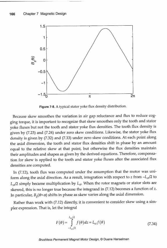
Figure 7-8. A typical stator yoke flux density distribution.

Because skew smoothes the variation in air gap reluctance and flux to reduce cog-ging torque, it is important to recognize that skew smoothes only the tooth and stator yoke fluxes but not the tooth and stator yoke flux densities. The tooth flux density is given by (7.23) and (7.24) under zero skew conditions. Likewise, the stator yoke flux density is given by (7.32) and (7.33) under zero skew conditions. At each point along the axial dimension, the tooth and stator flux densities shift in phase by an amount equal to the relative skew at that point, but otherwise the flux densities maintain their amplitudes and shapes as given by the derived equations. Therefore, compensa-tion for skew is applied to the tooth and stator yoke fluxes after the associated flux densities are computed.

In (7.12), tooth flux was computed under the assumption that the motor was uni-form along the axial direction. As a result, integration with respect to z from - L J 2 to LJ2 simply became multiplication by Lst. When the rotor magnets or stator slots are skewed, this is no longer true because the integrand in (7.12) becomes a function of z. In particular, Bg(0+a) shifts in phase as skew varies along the axial dimension.

Rather than work with (7.12) directly it is convenient to consider skew using a sim-pler expression. That is, let the integral

W2 F(0)= { f(8)dz = Lstf(0) ( 7 3 4 )

"i-s,/2

denote (7.12) where f(6) is the entire integrand of the outer integral. Moreover, if f(9) is represented by a Fourier series in electrical measure, (7.34) becomes

F(6) = LstJjFne'"e (7.35)

where F„ are the Fourier series coefficients of the integrand.

When the motor is skewed, (7.34) becomes

k,/2 f f(e,z)dz ( 7 3 6 )

where /(0,O)=/(0) as given by (7.34). In the usual case where skew is linear along the axial dimension, f(6,z) is described by applying a linear phase shift to the Fourier series in (7.35) that is proportional to the axial dimension, i.e.,

f(d,z)=JjF„e y L" (7.37)

in which a,; is the total skew in electrical measure. As written, the skew is -exJ2 at z=-Ls(/2, 0 at z=0, and aJ2 at z=Lsf/2. Substituting (7.37) into (7.36) and simplifying leads to

F s , (0) = L s ( £ s i n c ^ \Fne jnO (7.38)

Comparing this expression to (7.35), the influence of skew is given by the sinc(-) term in (7.38). That is, given the tooth flux Fourier series for the unskewed case (7.20) and (7.21), the tooth flux Fourier series coefficients for the skewed case <j>'tn are related to the coefficients in (7.21) by

<lhu - (7.39)

where S„ is the skew factor

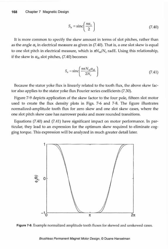
S„ = sine nac (7.40)

It is more common to specify the skew amount in terms of slot pitches, rather than as the angle a s in electrical measure as given in (7.40). That is, a one slot skew is equal to one slot pitch in electrical measure, which is KN,JNS radE. Using this relationship, if the skew is a - slot pitches, (7.40) becomes

S„ = sine 2 K (7.41)

Because the stator yoke flux is linearly related to the tooth flux, the above skew fac-tor also applies to the stator yoke flux Fourier series coefficients (7.30).

Figure 7-9 depicts application of the skew factor to the four pole, fifteen slot motor used to create the flux density plots in Figs. 7-6 and 7-8. The figure illustrates normalized-amplitude tooth flux for zero skew and one slot skew cases, where the one slot pitch skew case has narrower peaks and more rounded transitions.

Equations (7.40) and (7.41) have significant impact on motor performance. In par-ticular, they lead to an expression for the optimum skew required to eliminate cog-ging torque. This expression will be analyzed in much greater detail later.

Figure 7-9. Example normalized amplitude tooth fluxes for skewed and unskewed cases.

The ideal magnetic field distribution derived in Appendix B and summarized at the beginning of this chapter assumes that the ferromagnetic material in the motor is infi-nitely permeable. That is, it assumes that the field intensity H and the resulting MMF in the ferromagnetic portions of the motor are zero. In reality, the ferromagnetic por-tions have a finite permeability only one to three orders of magnitude greater than that of air. In addition, the permeability is a nonlinear function of the field strength. Because of the disparity between the assumed infinite permeability and the actual finite permeability, the magnetic field predicted in Appendix B over-predicts the amplitude of the magnetic field.

To compensate for the influence of ferromagnetic material, a reluctance factor simi-lar to that introduced in Chapter 4 is introduced. In this case, the reluctance factor modifies the amplitude but not the shape of the magnetic field. The approach fol-lowed here equates the MMF across the air gap under the ideal conditions assumed in Appendix B to the sum of the MMF across the actual air gap and the MMF across the finite permeability ferromagnetic material.

Implementing this approach requires two approximations. First, the MMF across the air gap is not constant over the surface of the magnet as shown in Fig. B-ll. Therefore, some specific air gap MMF must be used. Second, the magnetic field dis-tribution in the stator is not static. That is, it is a function of rotor position as illus-trated in Fig. 7-10. At the rotor position shown in the figure, the flux flowing in every third tooth does not travel out to the stator yoke but rather travels directly from one magnet to the next primarily through the shoe region of the tooth. As the rotor turns, each tooth experiences a varying magnetic field that causes the tooth reluctance to vary in response to the B-H curve of the tooth ferromagnetic material. Therefore, a particular rotor position must be chosen to find the reluctance factor.

The concepts behind the motor magnetic circuit model developed in Chapter 4 can be used to determine the reluctance factor by considering a one half magnet pitch section as shown between the dashed lines in the example motor cross section in Fig. 7-11. Here, a magnet pole is centered on a tooth on the right hand side of the figure. The flux flowing out of the magnet center crosses the air gap in a straight radial line. As a result, computation of the air gap MMF F„ along the magnet centerline is given simply as

(7.42)

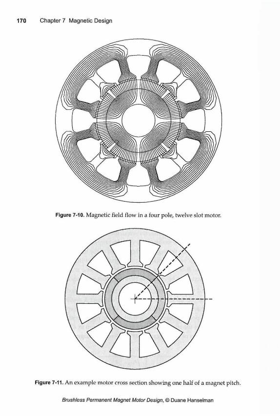
Figure 7-11. An example motor cross section showing one half of a magnet pitch.

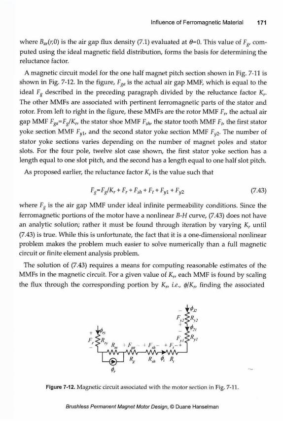
where Bar(r,0) is the air gap flux density (7.1) evaluated at 6=0. This value of Fg/ com-puted using the ideal magnetic field distribution, forms the basis for determining the reluctance factor.

A magnetic circuit model for the one half magnet pitch section shown in Fig. 7-11 is shown in Fig. 7-12. In the figure, Fgn is the actual air gap MMF, which is equal to the ideal Fg described in the preceding paragraph divided by the reluctance factor Kr. The other MMFs are associated with pertinent ferromagnetic parts of the stator and rotor. From left to right in the figure, these MMFs are the rotor MMF Fr, the actual air gap MMF Fga=Fg/Kr, the stator shoe MMF Fsh, the stator tooth MMF Ft, the first stator yoke section MMF Fyl, and the second stator yoke section MMF Fl/2. The number of stator yoke sections varies depending on the number of magnet poles and stator slots. For the four pole, twelve slot case shown, the first stator yoke section has a length equal to one slot pitch, and the second has a length equal to one half slot pitch.

As proposed earlier, the reluctance factor Kr is the value such that

Fg= Fg/Kr + Fr + Fsh + Ft + Fyi + Fy2 (7.43)

where Fg is the air gap MMF under ideal infinite permeability conditions. Since the ferromagnetic portions of the motor have a nonlinear B-H curve, (7.43) does not have an analytic solution; rather it must be found through iteration by varying Kr until (7.43) is true. While this is unfortunate, the fact that it is a one-dimensional nonlinear problem makes the problem much easier to solve numerically than a full magnetic circuit or finite element analysis problem.

The solution of (7.43) requires a means for computing reasonable estimates of the MMFs in the magnetic circuit. For a given value of Kr, each MMF is found by scaling the flux through the corresponding portion by Kr, i.e., <j)/Kr, finding the associated

Figure 7-12. Magnetic circuit associated with the motor section in Fig. 7-11.

flux density B by dividing the flux by the cross-sectional area of the portion, using the material's B-H curve to find the corresponding field intensity H, and finally multi-plying this field intensity by the flux path length of the portion to produce the required MMF, i.e., F=Hl.

The stator shoe and tooth fluxes are both given by 0f(O) in (7.20). The first stator yoke section flux is given by (7.29) and (7.30) evaluated at 9=0. The second stator yoke section is found by applying (7.31) to (7.29) or by simply evaluating (7.29) at 9=-9se. The rotor flux can be approximated by the tooth flux (7.20) <pt(0) as well. The cross-sectional areas and flux path lengths are easily approximated by mean geomet-ric values.

in the absence of an available numerical algorithm for the solution of (7.43), the solution can be found by employing the bisection algorithm, which can be described as follows. Two extreme estimates of the reluctance factor are chosen, e.g., Kr=1 and Kr=2. For each of these values, the difference between the two sides of (7.43) is found. Next, the mean or average of these Kr values is tested as well. The extreme estimate whose difference in (7.43) shares the same sign as the mean value is discarded and replaced by the mean value. Then a new mean value is computed, tested, and is used to replace one of the current extreme values. Through continued iteration of this algorithm, the range between the minimum and maximum Kr values is repeatedly bisected, eventually leading to an estimate of the reluctance factor.

When (7.43) is satisfied, the air gap flux density, rotor flux, shoe flux, tooth flux, and stator yoke fluxes are all divided by the reluctance factor Kr. For example, the Fourier series coefficients describing the tooth flux (7.21) become

A' _ 0/» K - — (7.44)

Typically, the reluctance factor falls between 1.0 and 1.1, meaning that the ideal air gap flux density computed in Appendix B over estimates the actual air gap flux den-sity between 0 and 10%. If the reluctance factor is greater than around 1.1, the ferro-magnetic portions of the motor consume too much MMF relative to the air gap, lead-ing to diminished motor performance.

Of the MMFs in (7.43), the stator tooth MMF is often much greater than all the other MMFs. This implies that the stator tooth plays a dominant role in how much the air gap flux density decreases. As a result, reducing the reluctance factor often means increasing the stator tooth width so that the corresponding field intensity and MMF are decreased.

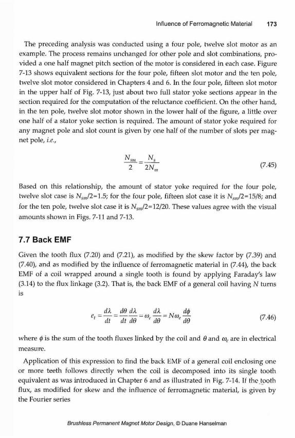
The preceding analysis was conducted using a four pole, twelve slot motor as an example. The process remains unchanged for other pole and slot combinations, pro-vided a one half magnet pitch section of the motor is considered in each case. Figure 7-13 shows equivalent sections for the four pole, fifteen slot motor and the ten pole, twelve slot motor considered in Chapters 4 and 6. In the four pole, fifteen slot motor in the upper half of Fig. 7-13, just about two full stator yoke sections appear in the section required for the computation of the reluctance coefficient. On the other hand, in the ten pole, twelve slot motor shown in the lower half of the figure, a little over one half of a stator yoke section is required. The amount of stator yoke required for any magnet pole and slot count is given by one half of the number of slots per mag-net pole, i.e.,

**m _ Ns

(7-45)

Based on this relationship, the amount of stator yoke required for the four pole, twelve slot case is Nsm/2=1.5; for the four pole, fifteen slot case it is Nsm/2=15/8; and for the ten pole, twelve slot case it is Nsm/2=12/20. These values agree with the visual amounts shown in Figs. 7-11 and 7-13.

7.7 Back EMF

Given the tooth flux (7.20) and (7.21), as modified by the skew factor by (7.39) and (7.40), and as modified by the influence of ferromagnetic material in (7.44), the back EMF of a coil wrapped around a single tooth is found by applying Faraday's law (3.14) to the flux linkage (3.2). That is, the back EMF of a general coil having N turns is

dX d6 dX dX dib e, = — = —— = w„— = Ncop— (7 AM ' dt dt dO 1 d6 e dd ( / A b )

where 0 is the sum of the tooth fluxes linked by the coil and 6 and cot, are in electrical measure.

Application of this expression to find the back EMF of a general coil enclosing one or more teeth follows directly when the coil is decomposed into its single tooth equivalent as was introduced in Chapter 6 and as illustrated in Fig. 7-14. If the tooth flux, as modified for skew and the influence of ferromagnetic material, is given by the Fourier series

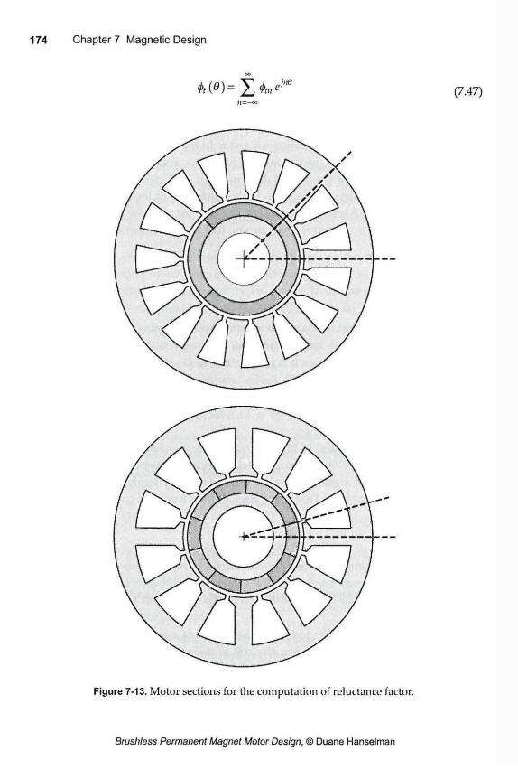
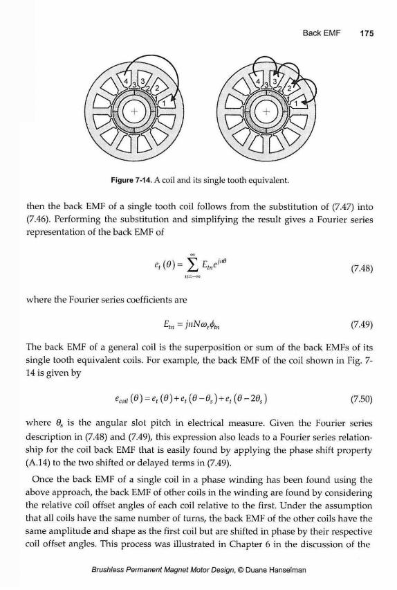
then the back EMF of a single tooth coil follows from the substitution of (7.47) into (7.46). Performing the substitution and simplifying the result gives a Fourier series representation of the back EMF of

oo et(d)=JjEtne'"e ( 7 4 g )

where the Fourier series coefficients are

Etn=jnNa>^tn (7.49)

The back EMF of a general coil is the superposition or sum of the back EMFs of its single tooth equivalent coils. For example, the back EMF of the coil shown in Fig. 7-14 is given by

(e) = et(d)+et(6-es) + et{6-2ds) (7.50)

where 9S is the angular slot pitch in electrical measure. Given the Fourier series description in (7.48) and (7.49), this expression also leads to a Fourier series relation-ship for the coil back EMF that is easily found by applying the phase shift property (A.14) to the two shifted or delayed terms in (7.49).

Once the back EMF of a single coil in a phase winding has been found using the above approach, the back EMF of other coils in the winding are found by considering the relative coil offset angles of each coil relative to the first. Under the assumption that all coils have the same number of turns, the back EMF of the other coils have the same amplitude and shape as the first coil but are shifted in phase by their respective coil offset angles. This process was illustrated in Chapter 6 in the discussion of the

winding factor for the case when all coils are connected in series. By using Fourier series to describe the tooth and coil back EMFs, it is straightforward to describe the phase back EMF epi,(0) in terms of Fourier series as well.

If the back EMF of phase A eph(6) is derived as described above, then the back EMF of phase B is epi,(0-6ph) and the back EMF of phase C is epi,(6-2dfli,)= €^,(6+0^,), where Qph=2nl?> radE. For a motor connected in the Y-connection as described in the next chapter, the line-to-line back EMF ea\,(6) measured between the terminals of phases A and B is

eM=eph(d)-eph(d-eph) (7.51)

The line-to-line back EMFs between the terminals of other phase combinations fol-lows accordingly. Using the delay and addition properties of Fourier series as dis-closed in Appendix A, the Fourier series description of the line-to-line back EMFs is easily related to that of the individual phase back EMFs.

7.8 Slotless Motor Construction

Although they do not appear often in applications, brushless permanent magnet motors can be constructed without stator teeth as illustrated in Fig. 5-2/?. This slotless construction cannot be analyzed using the single tooth equivalence that applies to slotted motors. This section addresses the slotless motor configuration by developing expressions for the flux linkage and back EMF.

Concentrated Winding Slotless motors exhibit no cogging torque, and therefore there is no need to utilize

fractional pitch coils or the equivalent of fractional slot construction. Furthermore, it is common to place coils side-by-side in the circumferential direction rather than forming two layers in the radial direction. As a result, slotless motors typically have full pitch coils and one coil per pole per phase, which is the equivalent of one slot per pole per phase. An example of this construction is shown in Fig. 7-15 where the four full-pitch coils of phase A associated with the four magnet poles are shown. The coils for phases B and C follow accordingly.

For three phase motors as shown in the figure, there are three coils per magnet pole with each coil having two coil sides. Therefore, there are six coil sides per magnet pole pitch. As a result, the angular distance allocated per coil side is

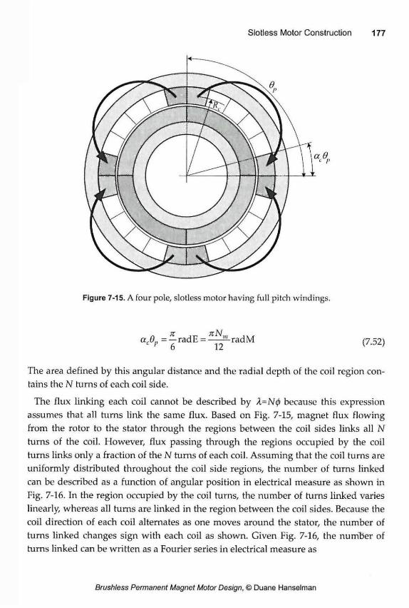
= |radE = LradM (7.52)

The area defined by this angular distance and the radial depth of the coil region con-tains the A/ turns of each coil side.

The flux linking each coil cannot be described by X=N<p because this expression assumes that all turns link the same flux. Based on Fig. 7-15, magnet flux flowing from the rotor to the stator through the regions between the coil sides links all N turns of the coil. However, flux passing through the regions occupied by the coil turns links only a fraction of the N turns of each coil. Assuming that the coil turns are uniformly distributed throughout the coil side regions, the number of turns linked can be described as a function of angular position in electrical measure as shown in Fig. 7-16. In the region occupied by the coil turns, the number of turns linked varies linearly, whereas all turns are linked in the region between the coil sides. Because the coil direction of each coil alternates as one moves around the stator, the number of turns linked changes sign with each coil as shown. Given Fig. 7-16, the number of turns linked can be written as a Fourier series in electrical measure as

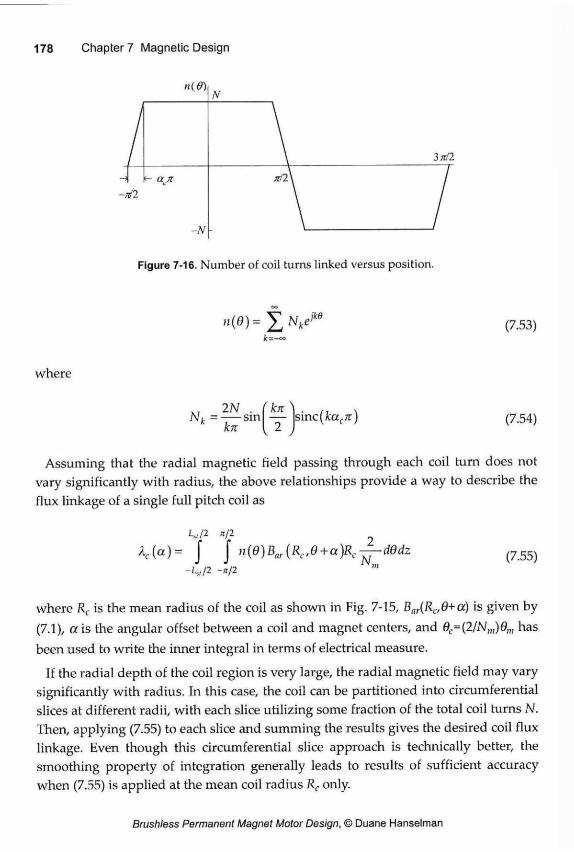
Figure 7-16. Number of coil turns linked versus position.

(7.53)

where

2N . f f e V , , v Nk = — sin — sine (kacn) (7.54)

Assuming that the radial magnetic field passing through each coil turn does not vary significantly with radius, the above relationships provide a way to describe the flux linkage of a single full pitch coil as

L,,/2 n/2 A c ( a ) = J j n(0)Bar{Rc,0+a)Rcjj-dedz ( 7 5 5 )

where Rc is the mean radius of the coil as shown in Fig. 7-15, Bar(Rc,d+a) is given by (7.1), « i s the angular offset between a coil and magnet centers, and Qc=(2/Nm)Qm has been used to write the inner integral in terms of electrical measure.

If the radial depth of the coil region is very large, the radial magnetic field may vary significantly with radius. In this case, the coil can be partitioned into circumferential slices at different radii, with each slice utilizing some fraction of the total coil turns N. Then, applying (7.55) to each slice and summing the results gives the desired coil flux linkage. Even though this circumferential slice approach is technically better, the smoothing property of integration generally leads to results of sufficient accuracy when (7.55) is applied at the mean coil radius Rc only.

Writing Bnr(Rc,d+a) as the Fourier series

Bar(Rc,e+a)=^Bgnei"^ ( 7 5 6 )

n=~oo

and substituting (7.56) and (7.53) into (7.55) leads to a coil flux linkage Fourier series

A c ( 0 ) = ] T V " e (7.57)

where

^ * HI (7.58)

where the variable substitution 9=a has been applied since A, is a function of electri-cal measure.

Assuming that all Nm coils are connected in series, and each coil has the same flux linkage, the phase flux linkage is simply the sum of that for each coil, or

A„,(0) = N m A c (0) (7.59)

The phase back EMF produced by this phase flux linkage is given by

= (7.60)

which, after substitution of (7.57) and (7.59) can be written as the Fourier series

É V " " (7.61)

where

En=jnNm(oeXn (7.62)

Use of (7.54), (7.56), and (7.58) into (7.62) and (7.61) gives the phase back EMF for a full pitch winding where the coils are concentrated.

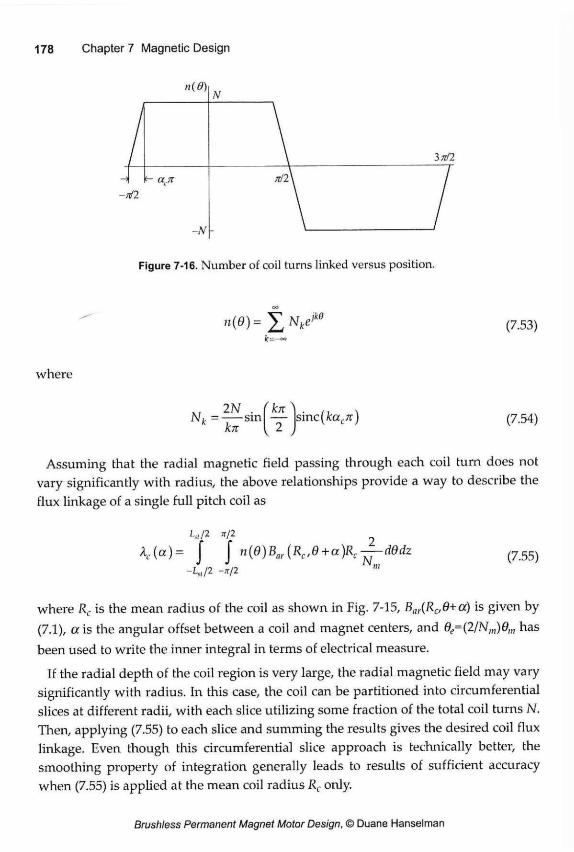
Figure 7-16. Number of coil turns linked versus position.

n ( d ) = J j N k e i k g (7.53) k=-

where

XI 2N . fkn \ . , Nk = — sin — sinc(tocJr) (7.54)

Assuming that the radial magnetic field passing through each coil turn does not vary significantly with radius, the above relationships provide a way to describe the flux linkage of a single full pitch coil as

W2 */2 Xc(oc)= J } n(d)Bar(Rc,e+a)Rc— dOdz ( 7 5 5 )

-Ls,/2 -n/2

where R( is the mean radius of the coil as shown in Fig. 7-15, B,jr(Rc,d+a) is given by (7.1), a is the angular offset between a coil and magnet centers, and 9e=(2/Nm)6m has been used to write the inner integral in terms of electrical measure.

If the radial depth of the coil region is very large, the radial magnetic field may vary significantly with radius. In this case, the coil can be partitioned into circumferential slices at different radii, with each slice utilizing some fraction of the total coil turns N. Then, applying (7.55) to each slice and summing the results gives the desired coil flux linkage. Even though this circumferential slice approach is technically better, the smoothing property of integration generally leads to results of sufficient accuracy when (7.55) is applied at the mean coil radius Rc only.

Writing Bnr(Rc,6+a) as the Fourier series

B f l f ( i ? c , 0 + a ) = j r V M 6 + a ) (7.56) h=-oo

and substituting (7.56) and (7.53) into (7.55) leads to a coil flux linkage Fourier series

¿ C ( 0 ) = X (7.57)

where

2nRcLsl . ( mn K = — ^ V 2 . N«->" s i n c — I (7.58)

' m

where the variable substitution 6= a has been applied since Xc is a function of electri-cal measure.

Assuming that all Nm coils are connected in series, and each coil has the same flux linkage, the phase flux linkage is simply the sum of that for each coil, or

Aph(B) = Nmlc(e) (7.59)

The phase back EMF produced by this phase flux linkage is given by

dXpjj *(*> = — ^ ( 7 ' 6 0 )

which, after substitution of (7.57) and (7.59) can be written as the Fourier series

eph(e)= I ; Ene'"e ( 7 6 1 ) »=-00

where

E„ = jnNmcoeXn (7.62)

Use of (7.54), (7.56), and (7.58) into (7.62) and (7.61) gives the phase back EMF for a full pitch winding where the coils are concentrated.

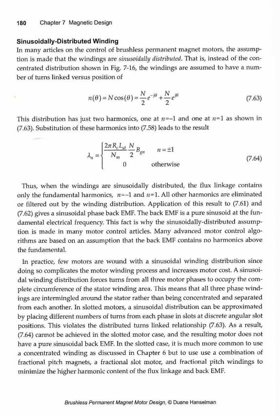
Sinusoidally-Distributed Winding In many articles on the control of brushless permanent magnet motors, the assump-tion is made that the windings are sinusoidally distributed. That is, instead of the con-centrated distribution shown in Fig. 7-16, the windings are assumed to have a num-ber of turns linked versus position of

This distribution has just two harmonics, one at »=-1 and one at n=1 as shown in (7.63). Substitution of these harmonics into (7.58) leads to the result

Thus, when the windings are sinusoidally distributed, the flux linkage contains only the fundamental harmonics, n=-1 and n=1. All other harmonics are eliminated or filtered out by the winding distribution. Application of this result to (7.61) and (7.62) gives a sinusoidal phase back EMF. The back EMF is a pure sinusoid at the fun-damental electrical frequency. This fact is why the sinusoidally-distributed assump-tion is made in many motor control articles. Many advanced motor control algo-rithms are based on an assumption that the back EMF contains no harmonics above the fundamental.

In practice, few motors are wound with a sinusoidal winding distribution since doing so complicates the motor winding process and increases motor cost. A sinusoi-dal winding distribution forces turns from all three motor phases to occupy the com-plete circumference of the stator winding area. This means that all three phase wind-ings are intermingled around the stator rather than being concentrated and separated from each another. In slotted motors, a sinusoidal distribution can be approximated by placing different numbers of turns from each phase in slots at discrete angular slot positions. This violates the distributed turns linked relationship (7.63). As a result, (7.64) cannot be achieved in the slotted motor case, and the resulting motor does not have a pure sinusoidal back EMF. In the slotted case, it is much more common to use a concentrated winding as discussed in Chapter 6 but to use use a combination of fractional pitch magnets, a fractional slot motor, and fractional pitch windings to minimize the higher harmonic content of the flux linkage and back EMF.

n(0) = Ncos(0) = — e~i°+ — e'0 (7.63)

ii — ¿1 (7.64)

0 otherwise

This chapter discloses techniques for solving the magnetic circuit for a general radial field motor, ultimately leading to expressions for the back EMF generated in the sta-tor windings due to the rotation of the rotor magnets. The magnetic field in the air gap was described in terms of a Fourier series whose coefficients were derived as the solution of partial differential equations with simple boundary conditions. From this solution, the influence of stator slots, the influence of skew, and the influence of the finite permeability of ferromagnetic material were considered. In each case, tech-niques were developed to compensate the ideal magnetic field distribution. Lastly, slotless motor construction was considered.

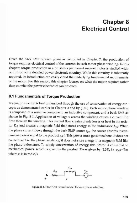
Given the back EMF of each phase as computed in Chapter 7, the production of torque requires electrical control of the currents in each motor phase winding. In this chapter, torque production in a brushless permanent magnet motor is studied with-out introducing detailed power electronic circuitry. While this circuitry is inherently required, its introduction can easily cloud the underlying fundamental requirements of the motor. For this reason, this chapter focuses on what the motor requires rather than on what the power electronics can produce.

8.1 Fundamentals of Torque Production

Torque production is best understood through the use of conservation of energy con-cepts as demonstrated earlier in Chapter 3 and by (3.43). Each motor phase winding is composed of a resistive component, an inductive component, and a back EMF as shown in Fig. 8-1. Application of voltage v across the winding causes a current i to flow through the winding. This current flow creates ohmic losses or heat in the resis-tor Rph and creates a magnetic field that stores energy in the inductance Lph. When the phase current flows through the back EMF source eph, the source absorbs instan-taneous power equal to the product ephi. This power must go somewhere. It does not create heat like the phase resistance; it does not store energy in a magnetic field like the phase inductance. To satisfy conservation of energy, this power is converted to mechanical power, which is given by the product Tco as given by (3.33), i.e., ephi=Tco, where (o is in radM/s.

L,

v

Figure 8-1. Electrical circuit model for one phase winding.

When a motor has more than one phase winding, conservation of energy must apply simultaneously for all phases. For three phase motors being considered here, this implies that

Tw-eaia+ebib+ecic (8.1)

where ev and ix for x=a,b, c are the respective back EMFs and currents in the three motor phases A, B, and C. Recognizing that the amplitudes of back EMFs are linearly proportional to speed co, the back EMFs in (8.1) can be written as ex=kxco where kx is the speed-independent shape of the back EMF having units of V/radM/s, which is equal to N-m/A. Substituting this relationship into (8.1) gives

T(e)=ka(0)iA6)+kb(e)ib(0)+kc(0)ic(0) (8.2)

where the position dependence of the torque, back EMF shapes, and currents has been shown explicitly.

In three phase motors with balanced windings, the back EMFs and currents of the three phases have the same shape but are offset by 0f,j,=27r/3radE or 120°E from each other. Using this fact, (8.2) can be rewritten as

T(0) = ka (6)itt [6) + ka ( 0 - e p h ) i a {0-0p!,) + ku (o+6ph)ia (0 +0„,) (8.3)

From this equation, it is clear that given the motor back EMF shape kn(d), torque pro-duction is determined solely by specifying the current shape in phase A, ia(0).

In practice, the desired torque is almost always a constant proportional to the amplitude of the current. That is, the motor should produce torque that does not vary as a function of position 0but does vary linearly with current amplitude. By follow-ing these desired characteristics, the motor becomes an easily-controlled source of torque that promotes optimum control of the load attached to the motor. The exis-tence of position dependent variations in the mutual torque, i.e., torque ripple, causes the motor load to repeatedly accelerate when the torque increases and decelerate when the torque decreases.

Given this description of the desired motor torque, the goal in choosing the phase A current shape ia(6) is to produce constant torque. In practice, this task has been accomplished by considering two "standard" back EMF shapes — trapezoidal and sinusoidal. When the motor has a trapezoidal back EMF, the motor is often referred to as a brushless DC motor, whereas when the back EMF is sinusoidal, the motor is

often referred to as a permanent magnet synchronous motor. There is nothing magi-cal about these terms. The fundamentals of torque production are identical, although the mathematics used to describe the two motors may be dramatically different. His-torically, the two motors originated from different areas. The term brushless DC motor comes from the fact that a brushless DC motor approximates the operation of a permanent magnet brush DC motor with power electronics taking the place of the brushes. The term permanent magnet synchronous motor describes an AC synchro-nous motor whose field excitation is provided by permanent magnets. Because of this difference in origin, the two motors are often mistakenly assumed to be much different from one another. What is different is the mathematics customarily used to describe them. The brushless DC motor is described in terms such as a torque con-stant and back EMF constant, whereas the permanent magnet synchronous motor is described in terms such as a rotating air gap MMF, synchronous reactance, and vec-tor control using a coordinate system based on direct and quadrature axes.

In the sections that follow, each of these motor types will be discussed as well as the general case where the back EMF is represented by a Fourier series.

8.2 Brushless DC Motor Drive Ideal Torque Production As stated earlier, a brushless DC motor generally describes a motor having a trape-zoidal back EMF. For this case, the phase currents are rectangular pulses, sometimes loosely identified as squarewave currents. While (8.3) can be used to describe torque production for this motor, it is easier to understand this configuration graphically as shown in Fig. 8-2, where the three phases have been labeled A, B, and C respectively.

In the figure, the back EMF shapes, i.e., the back EMFs divided by speed, are trape-zoids having 2/3 duty cycle. That is, for each 180°E the back EMF shape is constant over 120 °E. The current associated with each back EMF is composed of rectangular pulses having a 2/3 duty cycle, where the nonzero portions of the pulses are aligned with the flat areas of the respective back EMF shapes and the polarity of the current matches that of the back EMF. Following (8.2), the constant torque produced is shown at the bottom of the figure. Over each 60°E segment, positive current flows in one phase, negative current flows in another, and no current flows in the third phase. The letters below the constant torque line signify the two phases carrying current, with the overbar denoting negative current flow or flow out of a phase. Every 60°E, where the back EMF in a phase makes a transition, the current in one phase remains unchanged, while the current in another goes to zero, and the current in the third

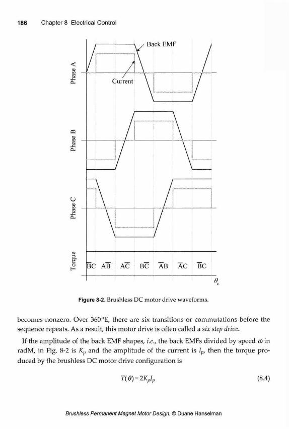
as 4= Q-

u « S3

CU

1) CT" Ö H BC AB AC BC AB AC BC

Figure 8-2. Brushless DC motor drive waveforms.

becomes nonzero. Over 360°E, there are six transitions or commutations before the sequence repeats. As a result, this motor drive is often called a six step drive.

If the amplitude of the back EMF shapes, i.e., the back EMFs divided by speed co in radM, in Fig. 8-2 is Kp and the amplitude of the current is Ip, then the torque pro-duced by the brushless DC motor drive configuration is

T( 6) = 2KpJp (8.4)

That is, the torque is constant and proportional to the current amplitude. The factor of two in (8.4) appears because two phases produce a torque equal to Kf,I}, at all instants.

The fundamental appeal of this brushless DC motor drive configuration is that position feedback need only identify the commutation points every 60°E. As a result, three simple Hall effect devices can be used to identify the commutation points. If the Hall effect devices are properly aligned with the back EMFs, processed Hall effect device signals can easily produce logic signals whose transitions occur at the desired commutation points.

Motor Constant Given the torque produced in (8.4), the motor constant K,„ for the brushless DC motor configuration can be found by computing the / R losses incurred. The RMS value of the ideal rectangular pulse currents shown in Fig. 8-2 is given by

(8.5)

This current flows through all three phase resistances producing total l2R losses of

P = 3lLRpl, (8.6)

Substituting (8.4) and (8.6) into the motor constant expression (4.40) gives

This expression shows that the motor constant is directly proportional to the ampli-tude of the back EMF shape, or back EMF constant. Since this analysis applies to the ideal case that cannot be achieved in practice, (8.7) represents the maximum achiev-able motor constant. Real brushless DC motor drive configurations will exhibit a somewhat lower motor constant.

Torque Ripple The biggest disadvantage of the brushless DC motor drive configuration is the physi-cal inability to generate the ideal rectangular pulse currents. As shown in the figure, the currents must make the required transitions instantaneously. In reality, the transi-tions require finite time. As a result, torque ripple is created at each commutation

point during the finite transition time of each phase current. This torque ripple is known as commutation torque ripple.

In addition to significant commutation torque ripple, the brushless DC motor drive configuration produces torque ripple whenever the back EMF or current shapes devi-ate from their ideal characteristics shown in Fig. 8-2. For example, if the back EMF or current shapes do not have a uniform amplitude from phase to phase or are not flat over the desired 120 °E intervals when torque is produced, torque ripple appears.

Because torque ripple is difficult to eliminate in the brushless DC motor drive con-figuration, it is seldom used in applications where minimum torque ripple is required. However, in velocity applications such as fans and pumps where motor speed and inertia are sufficiently high, torque ripple has little affect because of the inherent filtering provided by the inertia.

8.3 AC Synchronous Motor Drive

Ideal Torque Production

As stated earlier, an AC synchronous motor exhibits a sinusoidal back EMF shape, where the back EMF shape is the back EMF divided by speed CO in radM. In this case, if the back EMF and current shapes of phase A are respectively written as

ka(9) = Kpcos(G)

ia(9) = Ipcos(9) <8-8)

then, (8.3) becomes

T(9) = Kplp [cos2 (6) + cos2 (d -0ph ) + cos2 (fl + 9ph )] = | K p I p ( 8 .9)

As with the ideal brushless DC motor drive, constant torque with no torque ripple is produced. Here, matching the sinusoidal back EMF shape with a sinusoidal current shape aligned or in phase with the back EMF leads to constant torque whose ampli-tude is linearly proportional to the current amplitude Ip.

Compared to the discontinuous rectangular pulse currents required for the brush-less DC motor drive configuration, the sinusoidal currents in the AC synchronous motor drive configuration are continuous and infinitely differentiable. As a result, it is generally easier to produce sinusoidal currents and therefore easier to minimize

torque ripple in this case. On the other hand, production of sinusoidal currents requires more position information than that provided by three Hall effect sensors. In the AC synchronous motor case, position information is required throughout the electrical period, not just at the six commutation points needed in the brushless DC motor drive case. Traditionally, this position information has been provided by a resolver or position encoder. The expense and complexity incurred by using a resolver or encoder is easily justified in position control applications where the posi-tion sensor provides feedback for control purposes as well. In velocity control appli-cations, the need for these physical sensors can often be eliminated by employing digital signal processing algorithms to produce estimated position information of sufficient accuracy.

Motor Constant Given the ideal torque (8.9) and the RMS value of the phase current l m s = l H l , the motor constant Km of an ideal AC synchronous motor drive is

Thus, for the same amplitude back EMF shape, the motor constant for the AC syn-chronous motor drive is about 87% that of the ideal brushless DC motor drive as given by (8.7). While this may be disappointing given all the beneficial characteristics of the AC synchronous motor drive, this drop in motor constant appears because the brushless DC motor drive utilizes more harmonic content in both the back EMF and currents to produce torque.

Torque Ripple Since analytic expressions exist for the back EMF shape and current for the AC syn-chronous motor drive, it is possible to consider sources of torque ripple analytically. There are a number of possible imperfections in the back EMF or current that lead to torque ripple.

First, consider the situation where one back EMF amplitude or one current ampli-tude does not match the other phases. That is, let the amplitude of the back EMF or current in phase A be a factor of (1+A) greater than ideal. In this case, (8.9) becomes

(8.10)

T(0) = KpIp[( 1 + A)cos2 (0 ) + cos2 ( 0 - 9 p h ) + cos2 (d + 0,,,)]

= ^ V p + f V p c o s ( 2 0 ) 3 +A (8.11)

Thus, the constant torque produced has increased to (3+A)KpIp/2 and a torque ripple term at the second harmonic of the fundamental electrical frequency appears with an amplitude of AKpIp/2. The ratio of the amplitude of the torque ripple to the constant torque produced is

A A

Using this expression, a 3% amplitude error in one phase produces a peak torque ripple of approximately 1 %.

A second source of torque ripple occurs when the phase offset of a back EMF or current shape deviates from the ideal 0/,;,=2;r/3radE or 120°E offset among phases. For example, let the current in phase A be ¡¡,(6) = lpcos(d+S), where 5 is the angular mismatch. With this modification, (8.9) becomes

T (0) = KpIp [cos(0)cos(0 + 5) + cos2 (0 - 9 p h ) + cos2 (0 + Qph)] (8.13)

which for small ¿becomes

T ( 0 ) - | i C p i p + | K p / p s i n ( 2 0 ) (8.14)

Therefore, a misaligned back EMF or current also produces a second harmonic torque ripple component. In this case, the relative size of the torque ripple is 5/3 or one third, meaning that a 0.03rad (=1.72°) phase misalignment produces 1% peak torque ripple.

A third possible source of torque ripple occurs when either the back EMF or current shape contains harmonic terms in addition to the ideal fundamental terms in (8.8). To explore this possibility, let the back EMF shape of all phases contain a single higher harmonic having the form

k„( 9) = Kp cos( 0)+K„cos(n 9)

where n is an odd integer greater than 1. (Only odd integers need be considered, since they are the only terms that exist when the back EMF shape has halfwave sym-metry.) In this situation, (8.9) can be written as

T(0) = |K,,/p+ix„/ f , { l + 2cos[ ( ; ! - l )0 f l / , ] }cos[ (n- l )0]

+ lK, ,/ f , { l+2cos[(»+l)0p„]}cos[(» + l ) e ] ( 8 " 1 5 )

As shown in this equation, the addition of a single harmonic to the back EMF or cur-rent shape of all phases introduces two torque harmonics, one at the (n-l)th har-monic and another at the (n+l)th harmonic. The amplitudes of these torque harmon-ics are determined by the value of the two terms {l+2cos[(;i±l)0p/,]}. For 8ph=2k/ 3radE, (l+2cos[(«-l)0p;,]| is nonzero and equal to 3 for n equal to odd integers 6(7+1, for any positive integer q. Similarly, (l+2cos[(n + l)0p/,]| is nonzero and equal to 3 for n equal to odd integers 6q-l, for any positive integer q. This implies that if n is any odd integer other than a multiple of three, torque ripple is produced, and the amplitude of the torque ripple is equal to 3K„lp/2.

A final potential source of torque ripple to consider is phase misalignment between all back EMF and current shapes. In this case, let all currents be shifted in phase by S from their ideal angles, e.g., i„(9)=lpcos(9-S). With these modifications, (8.9) becomes

T(0) = |K p I p cos(5) (8.16)

In this case, no torque ripple is produced, but the torque amplitude is scaled by cos(<5). Although no torque ripple appears, the torque production becomes less effi-cient, since the current amplitude and resulting I R losses remains unchanged.

This phase misalignment between all back EMF and current shapes provides one way to illustrate vector control or field-oriented control concepts, which are com-monly used in motor control algorithms implemented using digital signal processors. Vector control expresses motor quantities in terms of quadrature and direct compo-nents. If the motor currents are misaligned by an angle 8 as considered in the pre-ceding passage, the currents can be written as

ia {9) = Ip cos (9 - 5) = Iq cos (0) +1d sin (9)

ib (9) = Ip c o s ( 9 - 9 p h - S ) = J, cos(0-9p„)+/,, sin(0 -9ph)

ic (9) = Ip cos(d+9ph - 5 ) = Iq cos(9 +9ph) + Id s in (9+9p h )

where

Iq = I p cos (5) (8.18)

is the quadrature component of the current and

Id=Ip sin(S) (8.19)

is the direct component of the current. Based on this description (8.16) becomes

The quadrature and direct components are constants that describe the amplitude of variables in terms of a quadrature component that is in phase with the back EMF and a direct component that is 90°E out of phase with the back EMF. (Since the term quadrature means "to be perpendicular to" these definitions appear to be backwards. They are defined as above, because quadrature and direct are in reference to the flux linkage, e.g., if the flux linkage is Asin(0), then the back EMF is ©Acos(0), and the direct term Id is in phase with the flux linkage, and the quadrature term is 90° out of phase with the flux linkage.)

In vector control, the instantaneous motor phase currents are processed by multipli-cation by a dq transformation matrix to produce L and ld. The difference between these values and their respective desired values creates error signals that are used in control loops to drive the actual currents to the desired values.

Since the direct component Id does not appear in the torque equation (8.20) but does contribute to ohmic losses, it is usually driven to zero by vector control algorithms. However, at high speeds where the back EMF amplitudes become larger than the voltage used to drive the motor, it becomes increasingly difficult to generate motor currents that lead to usable torque. This occurs because the rate of change in phase current as described by the phase winding model shown in Fig. 8-1 is given by

As the peaks in the back EMF eph reach or exceed the applied voltage v, it becomes difficult or impossible to increase the phase current, i.e., to make di/dt>0. In this situa-tion, motor currents must be increased before the respective peaks of the back EMFs appear. That is, the motor currents must be advanced in phase relative to their back

n0)=4v< 2 P i (8.20)

di _ v-tpi, -Rpiji dt ~ Lp„ (8.21)

EMFs. In vector control, this means making <5 negative, which creates a negative direct component to the current, i.e., ¡¡¡<0. This is commonly referred to as field or flux weakening control above base speed.

8.4 General Drive

Ideal Torque Production In addition to the two common drive configurations just discussed, insight can be gained by considering the general drive case where the back EMF and current shapes have arbitrary shapes. For this situation, let the back EMF and current shape for phase A be written as the Fourier series

oo

kl,(6)=JjKne'"e

n=-oo

hj=-m

Substitution of these expressions into (8.3) and simplifying gives a Fourier series description of the motor torque as

T(0)= X r n [ l + 2cos(2™/3)y n 0 ( 8 2 3 )

where r„ is the nth Fourier series coefficient of the torque produced by phase A

xn = X ^mhi-m (8.24)

Despite the apparent complexity of (8.23) and equation (8.24), the use of the exponen-tial form of the Fourier series makes the above expressions much simpler than equivalent expressions using either of the trigonometric forms of the Fourier series.

Equation (8.24) shows that the torque Fourier series coefficients are related to those of the back EMF and current by a convolution summation. Thus, each phase current harmonic contributes to all torque harmonics. The cross product of individual cur-rent and back EMF harmonics contributes to torque harmonics at frequencies equal to the sum and difference of the individual current and back EMF harmonics. This was demonstrated earlier in (8.14).

Evaluation of the term in brackets in (8.23) and (8.24) for various 11 gives the har-monic content of the motor torque. For example, the constant or average torque is given by the n=0 component

T0 = T„ [ l + 2cos(0)] = 3 £ KmI_m ( 8 2 5 ) hl=-oo

This equation illustrates that the average torque produced by the motor is the sum of all products of opposite harmonics in the phase current and back EMF. Therefore, if the back EMF does not have a qth harmonic, the existence of a qth current harmonic does not add to the usable average torque but does add to the ohmic losses, since the mean square value of the phase current is

£ » = ( ' ( 0 ) 2 ) = X l ' « | 2 (8.26)

Clearly, to maximize the motor constant, current harmonics should be zero whenever the corresponding back EMF harmonic is zero. Moreover, to maximize torque pro-duction efficiency, current harmonics should be large when the corresponding back EMF harmonic is large. In addition, (8.25) shows that increasing the harmonic con-tent of both the back EMF and current offers the possibility of maximizing torque production. The

more nonzero terms that exist in (8.25), the greater the average torque produced. This explains why the torque produced by the brushless DC motor drive is greater than that produced by the AC synchronous motor drive for the same amplitude back EMF and current. The AC synchronous motor drive utilizes only the fundamental component of the back EMF and current, whereas the back EMF and current in a brushless DC motor drive have substantial harmonic content beyond the fundamental.

Further simplification of (8.23) and (8.24) is possible. The term in brackets in (8.23), is nonzero and equal to 3 only when n is a multiple of three. All

other terms are zero. As a result, the motor torque only has harmonics at indices that are multiples of three. These harmonics are often called triple-« or triplen harmonics. Furthermore, since the back EMF and current exhibit half wave symmetry, all of the even harmonics of both the back EMF shape and current are zero. When this is true, the convolution summation in (8.24) is zero for all odd indices n. Combining this with the previous result, the motor torque contains only harmonics that are multiples of six. That is, (8.23) can be rewritten as

(8.27)

where

7*6» ~ 3 X Km lè n_n (8.28)

Torque Ripple The existence of torque ripple due to harmonic mismatch between the back EMF shape and the current is described by (8.27) and (8.28). For example, the torque har-monic amplitudes at six times the electrical frequency are given by the T_f, and T6

Fourier series coefficients

T-6 -••• + K_sI_j + K_3L3 + K_J_5 + Kxl_7 + K3I_g + K5I_n +•••

T6 = • • • + K_5/i I + K-3'9 + K-i /7 + + K373 +K5I_l+- ( 8 ' 2 9 )

If these sums are nonzero, torque ripple exists at the sixth harmonic. On the other hand, if the current harmonics are chosen properly, these sums can be set to zero, thereby eliminating torque ripple at the sixth harmonic. It can be shown that any number of torque harmonics can be simultaneously eliminated by proper selection of current harmonics. In fact, the selection of current harmonics is not unique. There are an infinite number of zero torque ripple solutions. Of these, the optimum choice is the set of current harmonics that simultaneously minimizes the RMS value of the cur-rent as given by the square root of (8.26). This choice maximizes torque production efficiency by maximizing the motor constant. Detailed analytic treatment of this zero torque ripple solution can be found in journal articles listed in the Bibliography.

Motor Constant In this general drive case, the motor constant cannot be expressed in a simple form where the current cancels between the numerator and denominator. Using (8.25) and (8.26) the motor constant can be written as

00

3

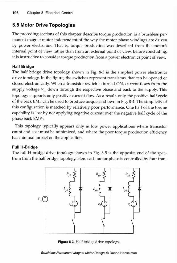
8.5 Motor Drive Topologies The preceding sections of this chapter describe torque production in a brushless per-manent magnet motor independent of the way the motor phase windings are driven by power electronics. That is, torque production was described from the motor's internal point of view rather than from an external point of view. Before concluding, it is instructive to consider torque production from a power electronics point of view.

Half Bridge The half bridge drive topology shown in Fig. 8-3 is the simplest power electronics drive topology. In the figure, the switches represent transistors that can be opened or closed electronically. When a transistor switch is turned ON, current flows from the supply voltage Vcc down through the respective phase and back to the supply. This topology supports only positive current flow. As a result, only the positive half cycle of the back EMF can be used to produce torque as shown in Fig. 8-4. The simplicity of this configuration is matched by relatively poor performance. One half of the torque capability is lost by not applying negative current over the negative half cycle of the phase back EMFs.

This topology typically appears only in low power applications where transistor count and cost must be minimized, and where the poor torque production efficiency has minimal impact on the application.

Full H-Bridge The full H-bridge drive topology shown in Fig. 8-5 is the opposite end of the spec-trum from the half bridge topology. Here each motor phase is controlled by four tran-

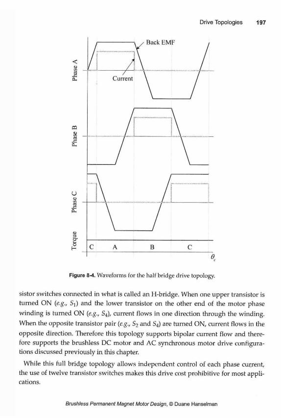
en Si ctì a.

U I Oh

u 3 cr b f— B C

Figure 8-4. Waveforms for the half bridge drive topology.

sisfor switches connected in what is called an H-bridge. When one upper transistor is turned ON (e.g., Sj) and the lower transistor on the other end of the motor phase winding is turned ON (e.g., S4), current flows in one direction through the winding. When the opposite transistor pair (e.g., S2 and S 4 ) are turned ON, current flows in the opposite direction. Therefore this topology supports bipolar current flow and there-fore supports the brushless DC motor and AC synchronous motor drive configura-tions discussed previously in this chapter.

While this full bridge topology allows independent control of each phase current, the use of twelve transistor switches makes this drive cost prohibitive for most appli-cations.

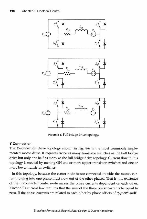
/-Connection The Y-connection drive topology shown in Fig. 8-6 is the most commonly imple-mented motor drive. It requires twice as many transistor switches as the half bridge drive but only one half as many as the full bridge drive topology Current flow in this topology is created by turning ON one or more upper transistor switches and one or more lower transistor switches.

In this topology, because the center node is not connected outside the motor, cur-rent flowing into one phase must flow out of the other phases. That is, the existence of the unconnected center node makes the phase currents dependent on each other. Kirchhoff's current law requires that the sum of the three phase currents be equal to zero. If the phase currents are related to each other by phase offsets of 0 ,=27r/3radE

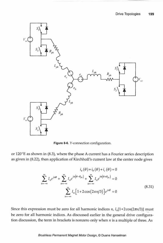
Figure 8-6. Y-connection configuration.

or 120°E as shown in (8.3), where the phase A current has a Fourier series description as given in (8.22), then application of Kirchhoff's current law at the center node gives

i8(0)+ib(0)+ic(e) = o j r i „ e ' n B + j r + j r 7 , / ^ = 0

/„[l+2cos(27TH/3)y"° =0 (8.31)

Since this expression must be zero for all harmonic indices n, 7„[l+2cos(2ro//3)] must be zero for all harmonic indices. As discussed earlier in the general drive configura-tion discussion, the term in brackets is nonzero only when n is a multiple of three. As

a result, for (8.31) to hold, the current cannot have any harmonics that are multiples of three. That is, the current cannot have triplen harmonics.

Certainly the AC synchronous motor drive satisfies this constraint since sinusoidal currents are the fundamental or «=±1 harmonics. Though not readily apparent mathematically, the brushless DC motor drive satisfies this current constraint as well. Graphically, Fig. 8-2 shows that current flows into one phase and out of another at all instants, and therefore Kirchhoff's current law is met at the center node.

Another way to look at the constraint imposed by Kirchhoff's current law is to rec-ognize that once two of the three phase currents are set, the third phase current must be equal to the negative sum of the first two. Therefore, all three phase currents can-not be independently controlled as they can in the full H-bridge configuration.

4-Connection As an alternative to the Y-connection, the three motor phases can be connected in a zl-connection topology as shown in Fig. 8-7. Here the three motor phases are con-nected to form a loop. As with the Y-connection, current flow is created by turning ON one or more upper transistor switches and one or more lower transistor switches in the figure.

In practice, the 4-connection is seldom used because the topology allows currents to circulate around the loop or A That is, independent of external currents created by the transistor switches, the three back EMF sources add together to support circulat-ing currents. This phenomena is identical to the current that can circulate among individual coils making up a phase winding when they are connected in parallel as shown in Fig. 4-32.

Ignoring the transistor switches in Fig. 8-7, a circulating current in the A is created by the sum of the back EMFs acting on the phase resistances and inductances. If the back EMF shapes are described by Fourier series as given by (8.22), then the sum of the back EMF shapes are given by

ka(0)+kl,(8) + kc(O)= £ Kne'"e + £ K,/<B-^K X | |=-oo U=—00 h=-°°

= ¿K„[l + 2cos(2xn/3)]e>"e ( 8 ' 3 2 )

When this sum is zero, no current circulates around the loop. Since [1 +2cos(27rn/3)| is nonzero only when n is a multiple of three, circulating current is created only when

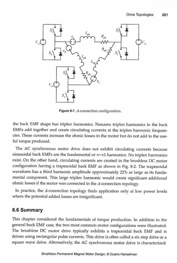
the back EMF shape has triplen harmonics. Nonzero triplen harmonics in the back EMFs add together and create circulating currents at the triplen harmonic frequen-cies. These currents increase the ohmic losses in the motor but do not add to the use-ful torque produced.

The AC synchronous motor drive does not exhibit circulating currents because sinusoidal back EMFs are the fundamental or «=±1 harmonics. No triplen harmonics exist. On the other hand, circulating currents are created in the brushless DC motor configuration having a trapezoidal back EMF as shown in Fig. 8-2. The trapezoidal waveform has a third harmonic amplitude approximately 22% as large as its funda-mental component. This large triplen harmonic would create significant additional ohmic losses if the motor was connected in the ^-connection topology.

In practice, the zi-connection topology finds application only at low power levels where the potential added losses are insignificant.

8.6 Summary

This chapter considered the fundamentals of torque production. In addition to the general back EMF case, the two most common motor configurations were illustrated. The brushless DC motor drive typically exhibits a trapezoidal back EMF and is driven using rectangular pulse currents. This drive is often called a six step drive or a square wave drive. Alternatively, the AC synchronous motor drive is characterized

by sinusoidal back EMFs and is typically driven by sinusoidal currents. This drive is often called a sinewave drive.

In addition to the fundamental of torque production, several basic power electronic drive topologies were illustrated. Of those discussed, the Y-connection overwhelm-ingly appears in applications.

This chapter focuses on motor performance. More specifically it focuses on providing guidance in the selection of magnet pole count Nm/ slot count Ns, and the ratio of the outside rotor radius Rw to the outside stator radius Rso. In addition, it develops pro-cedures for computing cogging torque, radial force, core losses, and AC winding resistance.

9.1 Motor Constant

As has been demonstrated in earlier chapters, motor constant describes the torque production efficiency of a motor that is independent of the number of turns per coil and the motor current. Therefore, motor constant provides valuable insight into maximizing motor performance.

General Sizing Before maximization of the motor constant is discussed, it is beneficial to identify how the dimensions of the ferromagnetic portions of the motor are related to the number of magnet poles, the number of slots, and the rotor outside radius. To sim-plify this discussion consider the motor cross section shown in Fig. 9-1, and let the air gap magnetic field distribution be ideal as shown in Fig. 4-5.

If one ignores the alternating direction of flux flow over alternating magnet faces, the total flux crossing the air gap in Fig. 9-1 can be written as

¿total = B A = Bg2nRr0Lit (9.1)

where B ? is the amplitude of air gap flux density and Lst is the axial stack length of the motor. This flux divides among the teeth and travels outward or inward depend-ing on which magnet polarity faces each tooth. As a result, the magnitude of the flux flowing in each tooth is

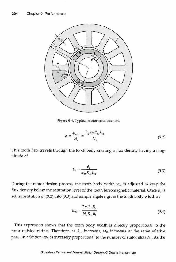
Figure 9-1. Typical motor cross section.

_<t>lotal _ B2nR r o L s t

This tooth flux travels through the tooth body creating a flux density having a mag-nitude of

D _ A

During the motor design process, the tooth body width zvth is adjusted to keep the flux density below the saturation level of the tooth ferromagnetic material. Once Bt is set, substitution of (9.2) into (9.3) and simple algebra gives the tooth body width as

2 nRwBg

This expression shows that the tooth body width is directly proportional to the rotor outside radius. Therefore, as Rr0 increases, z% increases at the same relative pace. In addition, wtb is inversely proportional to the number of stator slots Ns. As the

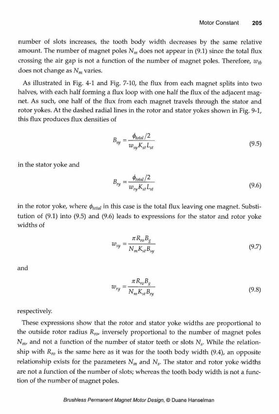
number of slots increases, the tooth body width decreases by the same relative amount. The number of magnet poles N,„ does not appear in (9.1) since the total flux crossing the air gap is not a function of the number of magnet poles. Therefore, wt{, does not change as Nm varies.

As illustrated in Fig. 4-1 and Fig. 7-10, the flux from each magnet splits into two halves, with each half forming a flux loop with one half the flux of the adjacent mag-net. As such, one half of the flux from each magnet travels through the stator and rotor yokes. At the dashed radial lines in the rotor and stator yokes shown in Fig. 9-1, this flux produces flux densities of

R 4W/2 V = ( 9 ' 5 )

in the stator yoke and

n L t d / 2

ry ' wryKslLsl (9-6)

in the rotor yoke, where <j>tolal in this case is the total flux leaving one magnet. Substi-tution of (9.1) into (9.5) and (9.6) leads to expressions for the stator and rotor yoke widths of

nR r oB s

W s v " N K>B (9-7)

and

xRroB* Wry ~ N K tB (9-8)

'" m st ury

respectively.

These expressions show that the rotor and stator yoke widths are proportional to the outside rotor radius Rro, inversely proportional to the number of magnet poles Nm, and not a function of the number of stator teeth or slots Ns. While the relation-ship with Rw is the same here as it was for the tooth body width (9.4), an opposite relationship exists for the parameters Nm and Ns. The stator and rotor yoke widths are not a function of the number of slots; whereas the tooth body width is not a func-tion of the number of magnet poles.

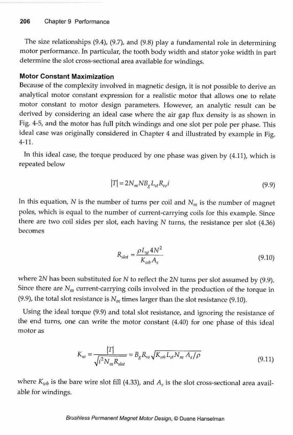
The size relationships (9.4), (9.7), and (9.8) play a fundamental role in determining motor performance. In particular, the tooth body width and stator yoke width in part determine the slot cross-sectional area available for windings.

Motor Constant Maximization Because of the complexity involved in magnetic design, it is not possible to derive an analytical motor constant expression for a realistic motor that allows one to relate motor constant to motor design parameters. However, an analytic result can be derived by considering an ideal case where the air gap flux density is as shown in Fig. 4-5, and the motor has full pitch windings and one slot per pole per phase. This ideal case was originally considered in Chapter 4 and illustrated by example in Fig. 4-11.

In this ideal case, the torque produced by one phase was given by (4.11), which is repeated below

\T\ = 2NmNBgLitRwi ( 9 . 9 )

In this equation, N is the number of turns per coil and Nm is the number of magnet poles, which is equal to the number of current-carrying coils for this example. Since there are two coil sides per slot, each having N turns, the resistance per slot (4.36) becomes

2 R

where 2N has been substituted for N to reflect the 2N turns per slot assumed by (9.9). Since there are Nm current-carrying coils involved in the production of the torque in (9.9), the total slot resistance is Nnl times larger than the slot resistance (9.10).

Using the ideal torque (9.9) and total slot resistance, and ignoring the resistance of the end turns, one can write the motor constant (4.40) for one phase of this ideal motor as

k ' " = ~ w s b = = ( 9 i d

where K w b is the bare wire slot fill (4.33), and A. is the slot cross-sectional area avail-able for windings.

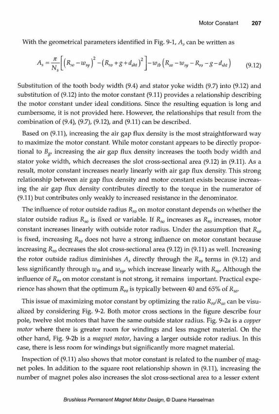
With the geometrical parameters identified in Fig. 9-1, As can be written as

K -wsy)2 -{Rro +g + dsi,t? -wtb (Rso-wsy-Rro-g-dM) (9.12) K

Substitution of the tooth body width (9.4) and stator yoke width (9.7) into (9.12) and substitution of (9.12) into the motor constant (9.11) provides a relationship describing the motor constant under ideal conditions. Since the resulting equation is long and cumbersome, it is not provided here. However, the relationships that result from the combination of (9.4), (9.7), (9.12), and (9.11) can be described.

Based on (9.11), increasing the air gap flux density is the most straightforward way to maximize the motor constant. While motor constant appears to be directly propor-tional to Bg, increasing the air gap flux density increases the tooth body width and stator yoke width, which decreases the slot cross-sectional area (9.12) in (9.11). As a result, motor constant increases nearly linearly with air gap flux density. This strong relationship between air gap flux density and motor constant exists because increas-ing the air gap flux density contributes directly to the torque in the numerator of (9.11) but contributes only weakly to increased resistance in the denominator.

The influence of rotor outside radius Rro on motor constant depends on whether the stator outside radius Rso is fixed or variable. If R s o increases as Rro increases, motor constant increases linearly with outside rotor radius. Under the assumption that Rso

is fixed, increasing Rro does not have a strong influence on motor constant because increasing Rro decreases the slot cross-sectional area (9.12) in (9.11) as well. Increasing the rotor outside radius diminishes A, directly through the Rro terms in (9.12) and less significantly through wtb and wsy, which increase linearly with Rw. Although the influence of Rr„ on motor constant is not strong, it remains important. Practical expe-rience has shown that the optimum Rr0 is typically between 40 and 65% of Rso.

This issue of maximizing motor constant by optimizing the ratio Rr0/Rs0 can be visu-alized by considering Fig. 9-2. Both motor cross sections in the figure describe four pole, twelve slot motors that have the same outside stator radius. Fig. 9-2a is a copper motor where there is greater room for windings and less magnet material. On the other hand, Fig. 9-2b is a magnet motor, having a larger outside rotor radius. In this case, there is less room for windings but significantly more magnet material.

Inspection of (9.11) also shows that motor constant is related to the number of mag-net poles. In addition to the square root relationship shown in (9.11), increasing the number of magnet poles also increases the slot cross-sectional area to a lesser extent

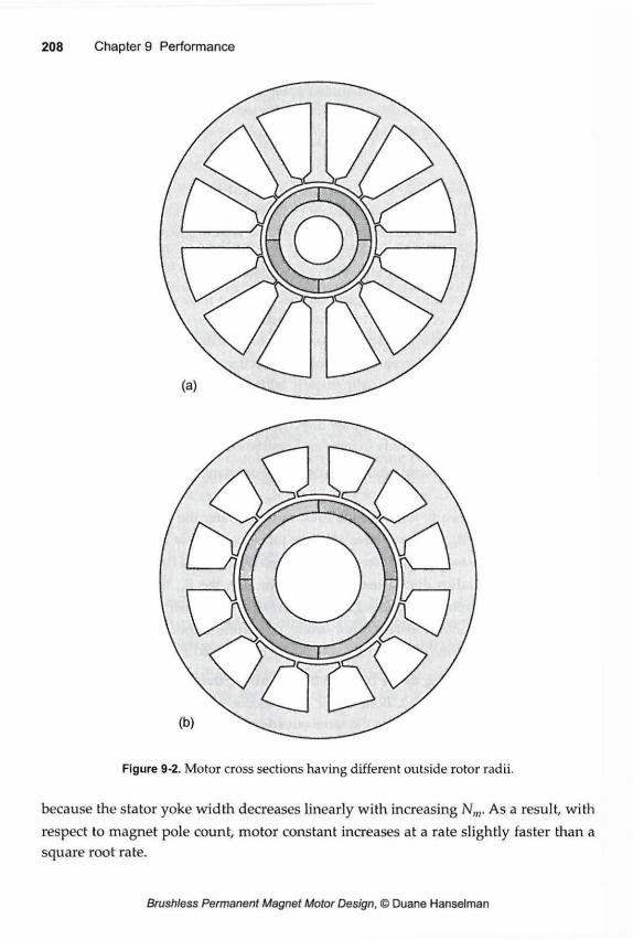
because the stator yoke width decreases linearly with increasing N,„. As a result, with respect to magnet pole count, motor constant increases at a rate slightly faster than a square root rate.

Motor constant as given by (9.11) ignores the winding end turns. Since the end turns create ohmic losses but do not produce torque, they directly diminish motor constant. This fact suggests that motor constant increases at a slightly greater rate with respect to Nm than that described in the preceding paragraph. This occurs because the length of the end turns are inversely proportional to the number of mag-net poles since the angular coil pitch is 2/r/iV„.radM. The presence of end turns also suggests that motor constant decreases somewhat with increasing outside rotor radius. This occurs because end turn length is directly proportional to the distance between slots, which increases somewhat with respect to Rr0 if Rso is fixed.

In summary, increasing the air gap flux density is the most significant way to increase motor constant. When the outside stator radius is fixed, the outside rotor radius plays an important but much less significant role in maximizing motor con-stant. Increasing the number of magnet poles plays a more significant role than the outside rotor radius but a less significant role than increasing the air gap flux density.

9.2 Cogging Torque Relationships

Cogging torque, as illustrated previously in Chapter 4, describes the desire of the permanent magnets on the rotor to align with a maximum amount of ferromagnetic material. In chapter four it was shown that integral slot motors have greater cogging torque than fractional slot motors. This occurs because the cogging torques created by the magnets add in phase alignment in integral slot motors, whereas they are out of phase with each other in fractional slot motors. In addition to identifying a num-ber of fundamental ways to minimize cogging torque, skewing the rotor magnets or stator slots was shown to minimize cogging torque.

The fundamental properties of cogging torque described in Chapter 4 can be used to quantify the relationship among magnet pole count N„„ slot count Ns, and skew. The cogging torques experienced by all stator teeth have the same shape, but are off-set from each other in phase by the angular slot pitch. Furthermore, cogging torque is periodic with respect to each magnet pole since South magnet poles create the same cogging torque as North magnet poles. As such, the fundamental frequency of the cogging torque is twice the fundamental electrical frequency whose period is one magnet pole pair. As a result, the cogging torque experienced by the kth stator tooth Tck(0) can be written as the Fourier series

T (f)\- V T Z 2 ! 8 " ^ ) 'ckWJ- 2 s 2 » e (9.13)

U=-co

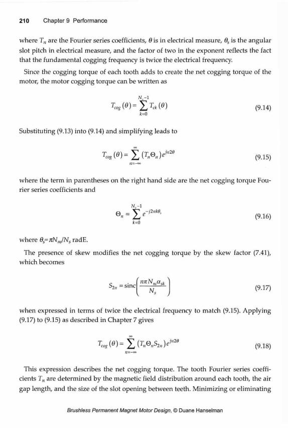
where T„ are the Fourier series coefficients, 8 is in electrical measure, 6i is the angular slot pitch in electrical measure, and the factor of two in the exponent reflects the fact that the fundamental cogging frequency is twice the electrical frequency.

Since the cogging torque of each tooth adds to create the net cogging torque of the motor, the motor cogging torque can be written as

n - 1

Tœg(9)= ^Tck(e) (9.14) fc=0

Substituting (9.13) into (9.14) and simplifying leads to

T C o g ( ° ) = t , m , ) e i " 2 6 (9.15)

where the term in parentheses on the right hand side are the net cogging torque Fou-rier series coefficients and

Qn = ]Te~f2'M' ( 9 A 6 ) k=0

where 6=7iNm/Ns radE.

The presence of skew modifies the net cogging torque by the skew factor (7.41), which becomes

( S2„ = sine

>viNmask (9.17)

when expressed in terms of twice the electrical frequency to match (9.15). Applying (9.17) to (9.15) as described in Chapter 7 gives

oo

^ ( 0 ) = X ( T » 0 » S 2 » ) e / " 2 < ' (9.18) J|=-oo

This expression describes the net cogging torque. The tooth Fourier series coeffi-cients Tn are determined by the magnetic field distribution around each tooth, the air gap length, and the size of the slot opening between teeth. Minimizing or eliminating

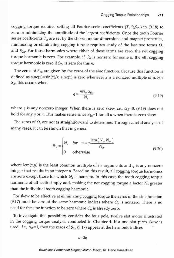
cogging torque requires setting all Fourier series coefficients (T„0„S2„) in (9.18) to zero or minimizing the amplitude of the largest coefficients. Once the tooth Fourier series coefficients T„ are set by the chosen motor dimensions and magnet properties, minimizing or eliminating cogging torque requires study of the last two terms 0„ and S2n. For those harmonics where either of these terms are zero, the net cogging torque harmonic is zero. For example, if Qn is nonzero for some n, the nth cogging torque harmonic is zero if S2n is zero for this n.

The zeros of S2n are given by the zeros of the sine function. Because this function is defined as sinc(x)=sin(x)/x, sinc(x) is zero whenever x is a nonzero multiple of n. For S2„ this occurs when

<7 = N~ (9.19)

where q is any nonzero integer. When there is zero skew, i.e., ask=Q, (9.19) does not hold for any q or n. This makes sense since S2„=l for all 11 when there is zero skew.

The zeros of 0„ are not as straightforward to determine. Through careful analysis of many cases, it can be shown that in general

0„ = lem ( N S / N J

N, for n = q — — N

(9.20) 0 otherwise

where lcm(x,i/) is the least common multiple of its arguments and q is any nonzero integer that results in an integer n. Based on this result, all cogging torque harmonics are zero except those for which 0„ is nonzero. In this case, the tooth cogging torque harmonic of all teeth simply add, making the net cogging torque a factor Ns greater than the individual tooth cogging harmonic.

For skew to be effective at eliminating cogging torque the zeros of the sine function (9.17) must be zero at the same harmonic indices where 0„ is nonzero. There is no need for the sine function to be zero where 0„ is already zero.

To investigate this possibility, consider the four pole, twelve slot motor illustrated in the cogging torque analysis conducted in Chapter 4. If a one slot pitch skew is used, i.e., 0^=1, then the zeros of S2n (9.17) appear at the harmonic indices

n=3q

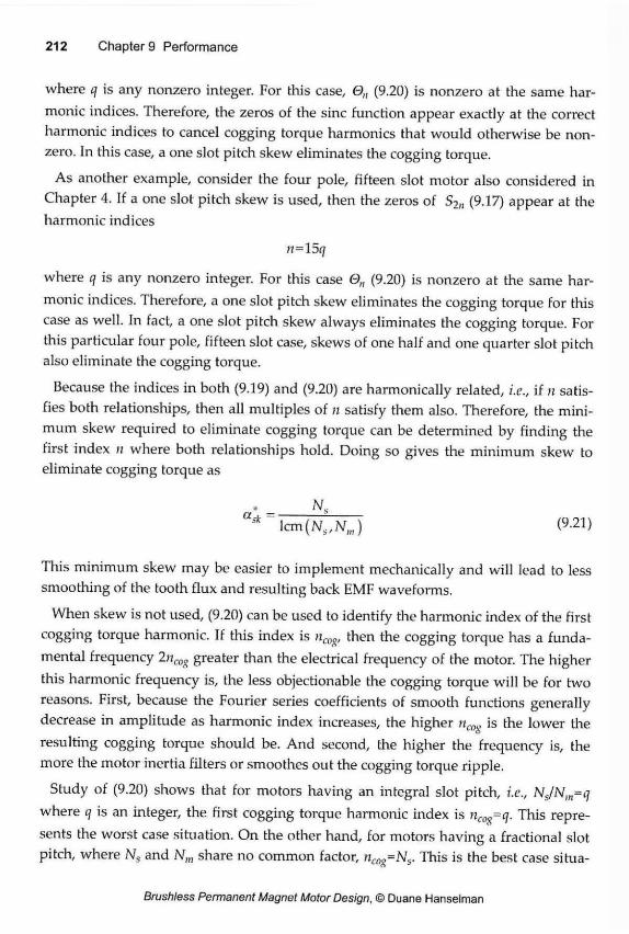
where q is any nonzero integer. For this case, 0„ (9.20) is nonzero at the same har-monic indices. Therefore, the zeros of the sine function appear exactly at the correct harmonic indices to cancel cogging torque harmonics that would otherwise be non-zero. In this case, a one slot pitch skew eliminates the cogging torque.

As another example, consider the four pole, fifteen slot motor also considered in Chapter 4. If a one slot pitch skew is used, then the zeros of S2„ (9.17) appear at the harmonic indices

n=\5q

where q is any nonzero integer. For this case 0„ (9.20) is nonzero at the same har-monic indices. Therefore, a one slot pitch skew eliminates the cogging torque for this case as well. In fact, a one slot pitch skew always eliminates the cogging torque. For this particular four pole, fifteen slot case, skews of one half and one quarter slot pitch also eliminate the cogging torque.

Because the indices in both (9.19) and (9.20) are harmonically related, i.e., if n satis-fies both relationships, then all multiples of n satisfy them also. Therefore, the mini-mum skew required to eliminate cogging torque can be determined by finding the first index n where both relationships hold. Doing so gives the minimum skew to eliminate cogging torque as

* Ns a*k lem (Ns,Nm) (9-21)

This minimum skew may be easier to implement mechanically and will lead to less smoothing of the tooth flux and resulting back EMF waveforms.

When skew is not used, (9.20) can be used to identify the harmonic index of the first cogging torque harmonic. If this index is ncog , then the cogging torque has a funda-mental frequency 2n c o g greater than the electrical frequency of the motor. The higher this harmonic frequency is, the less objectionable the cogging torque will be for two reasons. First, because the Fourier series coefficients of smooth functions generally decrease in amplitude as harmonic index increases, the higher ncog is the lower the resulting cogging torque should be. And second, the higher the frequency is, the more the motor inertia filters or smoothes out the cogging torque ripple.

Study of (9.20) shows that for motors having an integral slot pitch, i.e., NjNm=q where q is an integer, the first cogging torque harmonic index is ncog=q. This repre-sents the worst case situation. On the other hand, for motors having a fractional slot pitch, where Ns and Nm share no common factor, ncog=Ns. This is the best case situa-

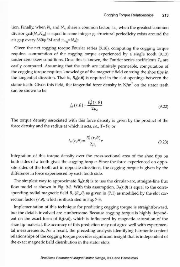
tion. Finally, when Ns and N„, share a common factor, i.e., when the greatest common divisor gcd(Ns,Nm) is equal to some integer p, structural periodicity exists around the air gap every 360/p°M and ncog=Ns/p.

Given the net cogging torque Fourier series (9.18), computing the cogging torque requires computation of the cogging torque experienced by a single tooth (9.13) under zero skew conditions. Once this is known, the Fourier series coefficients T„ are easily computed. Assuming that the teeth are infinitely permeable, computation of the cogging torque requires knowledge of the magnetic field entering the shoe tips in the tangential direction. That is, B^r,6) is required in the slot openings between the

stator teeth. Given this field, the tangential force density in N/m on the stator teeth

can be shown to be

= (9.22) ro

The torque density associated with this force density is given by the product of the force density and the radius at which it acts, i.e., T=Fr, or

, „x B o M ) i e M ) = (9.23)

Integration of this torque density over the cross-sectional area of the shoe tips on both sides of a tooth gives the cogging torque. Since the force experienced on oppo-site sides of the tooth act in opposite directions, the cogging torque is given by the difference in force experienced by each tooth side.

The simplest way to approximate Be(r,8) is to use the circular-arc, straight-line flux flow model as shown in Fig. 9-3. With this assumption, B^r,6) is equal to the corre-sponding radial magnetic field Bar(Rs,0) as given in (7.1) as modified by the slot cor-rection factor (7.9), which is illustrated in Fig. 7-3.

Implementation of this technique for predicting cogging torque is straightforward, but the details involved are cumbersome. Because cogging torque is highly depend-ent on the exact form of B^r,G), which is influenced by magnetic saturation of the shoe tip material, the accuracy of this prediction may not agree well with experimen-tal measurements. As a result, the preceding analysis identifying harmonic content relationships of the cogging torque provides significant insight that is independent of the exact magnetic field distribution in the stator slots.

£

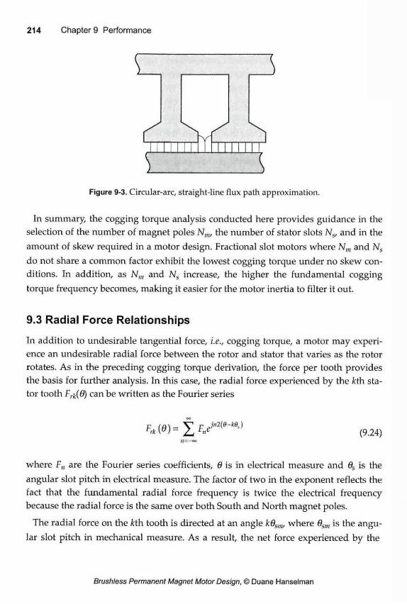
I Figure 9-3. Circular-arc, straight-line flux path approximation.

In summary, the cogging torque analysis conducted here provides guidance in the selection of the number of magnet poles Nm, the number of stator slots Ns, and in the amount of skew required in a motor design. Fractional slot motors where Nm and Ns

do not share a common factor exhibit the lowest cogging torque under no skew con-ditions. In addition, as N,„ and Ns increase, the higher the fundamental cogging torque frequency becomes, making it easier for the motor inertia to filter it out.

9.3 Radial Force Relationships

In addition to undesirable tangential force, i.e., cogging torque, a motor may experi-ence an undesirable radial force between the rotor and stator that varies as the rotor rotates. As in the preceding cogging torque derivation, the force per tooth provides the basis for further analysis. In this case, the radial force experienced by the kth sta-tor tooth Frk(6) can be written as the Fourier series

Frk(0)= £ F„e >2 (e-wy

(9.24)

where Fn are the Fourier series coefficients, 0 is in electrical measure and 9S is the angular slot pitch in electrical measure. The factor of two in the exponent reflects the fact that the fundamental radial force frequency is twice the electrical frequency because the radial force is the same over both South and North magnet poles.

The radial force on the kth tooth is directed at an angle kdsm, where Qsm is the angu-lar slot pitch in mechanical measure. As a result, the net force experienced by the

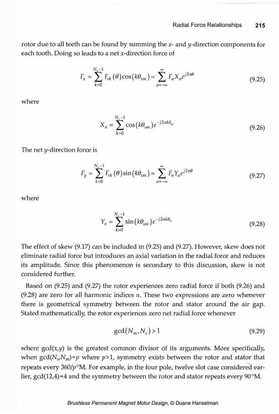
Radial Force Relationships 215

rotor due to all teeth can be found by summing the x- and y-direction components for each tooth. Doing so leads to a net x-direction force of

N.-L

= X F * ( 0 ) c o s ( f c 0 - ) = Z F " X " e i 2 " 9 (9.25) k=0

where

N.-l X„ = £ c o s (kdsm)e-i2"k0* ( 9 2 6 )

k=0

The net y-direction force is

N<-1 Fy = X Frk(0)sm(k6sm)= £ W 2 " 0 (9.27)

Jt=0

where

N,-1 Y„ = X sm(ke s ,nV i 2"k 0* (9.28)

t=o

The effect of skew (9.17) can be included in (9.25) and (9.27). However, skew does not eliminate radial force but introduces an axial variation in the radial force and reduces its amplitude. Since this phenomenon is secondary to this discussion, skew is not considered further.

Based on (9.25) and (9.27) the rotor experiences zero radial force if both (9.26) and (9.28) are zero for all harmonic indices n. These two expressions are zero whenever there is geometrical symmetry between the rotor and stator around the air gap. Stated mathematically, the rotor experiences zero net radial force whenever

gcd(N,„,Nj>l (9.29)

where gcd(x,y) is the greatest common divisor of its arguments. More specifically, when gcd(Ns,Nm)=^ where p> 1, symmetry exists between the rotor and stator that repeats every 360/p°M. For example, in the four pole, twelve slot case considered ear-lier, gcd(12,4)=4 and the symmetry between the rotor and stator repeats every 90°M.

Since the number of magnet poles is always an even number, there is zero net radial force whenever the number of slots is also an even number. Equation (9.29) is always met in this case. On the other hand, when the number of slots is an odd integer, the rotor experiences a net radial force whenever (9.29) is not met. For example, in a four pole, fifteen slot motor, gcd(15,4)=l and a net radial force exists. However, in a six pole, twenty-one slot motor, gcd(21,6)=3, and zero radial force exists.

In those cases where a net radial force appears, it is beneficial to know the harmonic indices that contribute to the net force since these indices identify the relative speed at which the net radial force rotates with respect to the rotor speed. The harmonic indices that contribute to the net radial force satisfy

(2q-l)Ns±l » - n ( 9 - 3 ° )

m

where q is a positive integer. The radial force at all other harmonic indices is zero. The harmonic indices that satisfy (9.30) do not exist for all q, nor are they uniformly spaced. For example, in a four pole, fifteen slot motor, the harmonics that satisfy (9.30) are n—4,11,19,26,..., where the difference between indices alternates between 7 and 8. For a ten pole, thirty-three slot motor, the harmonic indices that satisfy (9.30) are «=10,23,43,56,76,.. . , where the difference between indices alternates between 13 and 20. In both of these examples, the first contributing harmonic index is equal to Nm. However, this is not always true. For example, in an eight pole, twenty-slot motor, the harmonic indices that satisfy (9.30) are 77 = 10,17,37,44,.. . , where the first contributing index is 10 rather than 8.

In addition, it is true in general that the sum of the two numbers describing the alternating differences between indices for which nonzero radial force exists always equals the number of slots Ns. For example, in the four pole, fifteen slot motor the two numbers are 7 and 8, which sum to Ns=15.

When Xn in (9.26) is nonzero, it always equals NJ2. Similarly, when Yn in (9.28) is nonzero, it equals Ns/2 for those indices for which (9.30) is satisfied with the minus sign. And it equals -Ns/2 for those indices for which (9.30) is satisfied with the plus sign. For those cases in which radial force appears, it can be computed by determin-ing the radial force experienced by a single tooth. From the Fourier series coefficients of this force Fn, equations (9.25) through (9.28) give the desired net radial force in the x- and indirections. The radial force on one tooth can be computed by integrating the radial force density in N/m

Bj(Rs,9) ( 9 - 3 1 )

over the surface of a tooth. In (9.31), B^R^B) is given by (7.1) evaluated at the stator radius Rs at the air gap.

In summary, motors that do not have symmetry between the rotor and stator around the air gap will exhibit a net radial force having harmonic content above the fundamental electrical frequency of the motor. Since cogging torque is generally worse for motors having this symmetry, there is a tradeoff between minimum cog-ging torque and the presence of net radial force. In most applications, net radial force has little impact on performance. However, in low noise applications such as hard disk drive spindle motors, the presence of net radial force can limit motor acoustic performance.

9.4 Core Losses Basic Concepts In most motor designs, I R losses are the dominant contributor to reduced energy conversion efficiency. Core losses in the ferromagnetic portions of the motor are usu-ally the next largest contributor to motor losses. As described qualitatively in Chapter 2, core loss is the sum of hysteresis and eddy current losses. These two core loss com-ponents have been studied extensively for many years. Some studies have focused on understanding and modeling the phenomena at the atomic level. Others have focused on developing core loss expressions that facilitate core loss prediction in actual devices such as motors and transformers. Still others have focused on develop-ment of new material testing procedures that facilitate accurate curve fitting of meas-ured material properties to core loss expressions.

While the physical mechanisms that create core losses are well understood, applica-tion of this knowledge to make accurate core loss predictions remains difficult for a number of reasons. These reasons include:

• Core losses are created on a microscopic scale within a material, whereas core loss prediction uses a macroscopic scale based on assumptions of mag-netic field uniformity throughout regions of the device. Therefore, the accu-racy of core loss predictions depends on how well the chosen macroscopic regions model the material loss properties on a microscopic scale.

• Core loss data for many common materials is only available for 50 or 60Hz operation using sinusoidal excitation. This 50 or 60Hz excitation does not produce an assumed ideal sinusoidal magnetic field when using the data.

• Core loss data obtained from the commonly accepted Epstein Square Test is often of questionable value because standard test conditions do not match those of an actual motor.

• Material properties can vary by as much as 30% from batch to batch and within the same batch. In addition, they can vary within individual lamina-tions.

• Core loss is significantly influenced by the mechanical stress and strain experienced both within the material and on its surfaces and edges. For this reason, motor laminations are often annealed after being stamped or cut. Since core loss predictions uniformly ignore this material influence, core loss predictions for nonannealed or improperly annealed laminations are invariably inaccurate.

• Since the time variation of the magnetic field distribution within a motor is seldom sinusoidal, the accuracy of core loss predictions depends on how sinusoidal excitation data is used to generate core loss expressions that apply to nonsinusoidal magnetic fields.

• Core losses are easier to predict with accuracy in regions where only the amplitude of the magnetic field changes with time, e.g., in the stator tooth bodies and stator yoke sections. In regions where both the amplitude and angular direction of the magnetic field varies with time, an additional core loss component appears. That is, in addition to traditional hysteresis and eddy current loss components, the material exhibits additional rotational losses. This additional loss mechanism is highly dependent on the trajectory taken by the amplitude and angular motion of the magnetic field in a region. In a motor, these additional rotational losses are created in the tran-sition area between the stator teeth and the stator yoke. Studies have shown that rotational losses can double the core losses in a region. Because of the significant work required to identify magnetic field trajectories versus time and to convert this knowledge into viable core loss expressions that vary with the trajectory shape, rotational losses are often neglected or are crudely estimated.

• Some materials exhibit an additional loss component in addition to hystere-sis and eddy current components. This loss component, called the excess or

anomalous loss, is least understood, is difficult to determine from traditional core loss data, and is commonly ignored when predicting core losses.

Given all of these issues, core loss prediction using relatively simple modeling may indicate the correct trends from one motor design to the next but will not likely pro-duce accurate estimates of core losses at any given operating point.

Using knowledge of the fundamental principles that cause core losses, they can be reduced by:

• Reducing the lamination thickness. Ideally, eddy current losses are directly proportional to the square of the lamination thickness. Therefore, if lamina-tion thickness is reduced by a factor of two, eddy current losses decrease by a factor of four.

• Increasing the resistivity of the lamination material. Eddy current losses are inversely proportional to material resistivity. Adding silicon to lamination steel is the most commonly adopted approach to increasing material resis-tivity.

• Annealing laminations after they have been stamped or cut. This eliminates the influence of mechanical stress on core loss.

• Reducing the amplitude of the magnetic field within the material. Hystere-sis losses are directly proportional to the amplitude of the magnetic field raised to a power between 1.5 and 2.5. Eddy current losses are directly pro-portional to the square of the magnetic field amplitude. Using this property to reduce core loss is in direct conflict with maximizing torque production. As a result, other techniques for minimizing core losses are often imple-mented first.

• Reducing the number of magnet poles Nm. Hysteresis losses are directly proportional to the fundamental electrical frequency. Eddy current losses are directly proportional to the square of the fundamental electrical fre-quency. Since the fundamental electrical frequency is Nm/2 times greater than the motor shaft speed, reducing the magnet pole count allows one to reduce core losses significantly without lowering the motor shaft speed.

Core Loss Modeling With the preceding information in mind, this section illustrates one approach to esti-mating core losses in a motor. The process develops a core loss expression that is fit to standard core loss data. Then, using expressions for the stator tooth and yoke flux densities, core losses are estimated.

As stated in Chapter 2, hysteresis losses are typically characterized by

P/i -kufòpk (9.32)

where kh is a material dependent constant,/is the frequency of excitation, Bpk is the peak flux density, and n is a material dependent constant usually between 1.5 and 2.5. Since n varies somewhat with the flux density amplitude, it is convenient to include this in (9.32) as

where m is a material dependent constant. For materials having a given thickness, eddy current losses are typically characterized by

where kc is a material dependent constant that is proportional to the square of the material thickness. The sum of (9.33) and (9.34) is the core loss experienced by the material for a sinusoidal magnetic field having an amplitude of Bpk and frequency/.

In numerous studies, it has been shown that hysteresis losses are essentially inde-pendent of the magnetic field waveform shape. As a result, (9.33) remains unchanged for other magnetic field waveforms. On the other hand, (9.34) applies only when the magnetic field is sinusoidal in shape. In the general case, eddy current losses are pro-portional to the mean square value of the derivative of the magnetic field. That is, eddy current losses are proportional to the square of the RMS value of the derivative of the magnetic field. This makes sense because the voltage that creates the eddy cur-rents is related to dB/dt through Faraday's law (3.14). The square of the RMS value also makes sense because eddy current losses are I R losses, where J is the RMS value of the eddy currents. To understand how (9.34) must be changed, let

lh -KhJöpk (9.33)

Pe=Kf 2 B 2 p k (9.34)

B(t) = Bpksin{27tft) (9.35)

be the sinusoidal flux density in (9.34). The derivative of this expression is

-jp- = 2nfBpk cos(2K ft) (9.36)

for which the mean square value, or square of the RMS value is

'dB dt

= 2 n 2 f 2 B 2 p k ( 9 3 7 )

Rearranging this equation and substituting it into (9.34) leads to the more general expression for eddy current losses

* e In n ~Tt\ (9-38)

Given (9.33) and (9.34), core losses under sinusoidal excitation are

Pcore = P„ + Pc= KPT* + (9-39)

whereas, using (9.33) and (9.38), core losses under arbitrary excitation are

p _ p , p _ u . J w Éi. T lcore - l h + 1 e - KhJavk 2n2 dt (9.40)

Based on these two core loss expressions, the coefficients kju ke, n, and m in (9.39) are determined by fitting (9.39) to material data in W/kg or W/lb generated under sinu-soidal excitation conditions. Then, these coefficients are used in (9.40) to estimate core losses under nonsinusoidal excitation conditions.

There are a number of approaches that can be used to determine the coefficients kh, ke, n, and m in (9.39) and (9.40). Since there are four unknowns at least four data points are required to find a unique solution. Given that (9.39) does not match meas-ured data exactly, it is best to use numerous points and perform a least mean squares curve fit. This approach often leads to the best fit provided data points exist and are used that match the operating points / and Bpk expected in a motor. Since ke and k;, appear linearly iri (9.39), it is convenient to determine the coefficients by using linear least squares to find ke and k), after each iteration of a nonlinear algorithm for finding 7i and m. The goodness of any fit should be determined by comparing measured data to data generated by the evaluation of (9.39). In many cases, it is necessary to weight the data during the fitting process to produce a meaningful result. The mismatch between (9.39) and measured data is often a significant source of error in addition to the previously-cited reasons for difficulties and errors in core loss predictions.

Application to Motor Design Application of (9.40) for the estimation of core losses in motors is straightforward. If the magnetic field in a region is described by the Fourier series

b ( 6 ) = f j b y ' e ( 9 . 4 1 )

;j=-oo

where 6 is in electrical measure, then Bjlk is simply

Bpk=max(B(d)) (9.42)

Using (A.15), time derivative of (9.41) is

dB dddB v • R I'* (9-43)

where (Dc=2rfc. Applying (A.17), the mean square value of dB/dt is found as

( ( f ) } = 1 X I ^ B » | 2 (9.44)

Substitution of (9.42) and (9.44) into (9.40) gives the core loss density in W/kg or W/lb for the region whose flux density is given by (9.41). The frequency/in (9.40) is equal to the fundamental electrical frequency fe since that is the fundamental frequency of (9.41).

In a brushless permanent magnet motor, the permanent magnet field creates almost no core losses in the rotor yoke because time-varying flux is created only by the small variation in magnet operating point as magnet material passes over the stator slot openings. Flowever, both the stator teeth and yoke have flux densities that fit (9.41).

The stator tooth flux density is given by (7.23) and (7.24). Substituting this data into (9.41) gives the core loss density in the stator tooth body Multiplying this density by

3 3 3 3 the tooth volume in m or in and mass density in lb/in or kg/m and the number of teeth Ns, produces an estimate of the total core loss for the stator teeth. If desired, a separate calculation can be made for the stator shoe area based on an estimate of the flux density in the shoe region. This same procedure applies to the stator yoke, whose flux density is given by (7.32) and (7.33).

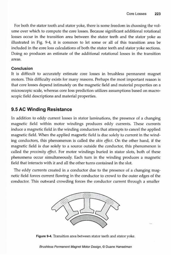
For both the stator tooth and stator yoke, there is some freedom in choosing the vol-ume over which to compute the core losses. Because significant additional rotational losses occur in the transition area between the stator teeth and the stator yoke as illustrated in Fig. 9-4, it is common to let some or all of this transition area be included in the core loss calculations of both the stator teeth and stator yoke sections. Doing so produces an estimate of the additional rotational losses in the transition areas.

Conclusion It is difficult to accurately estimate core losses in brushless permanent magnet motors. This difficulty exists for many reasons. Perhaps the most important reason is that core losses depend intimately on the magnetic field and material properties on a microscopic scale, whereas core loss prediction utilizes assumptions based on macro-scopic field descriptions and material properties.

9.5 AC Winding Resistance

In addition to eddy current losses in stator laminations, the presence of a changing magnetic field within motor windings produces eddy currents. These currents induce a magnetic field in the winding conductors that attempts to cancel the applied magnetic field. When the applied magnetic field is due solely to current in the wind-ing conductors, this phenomenon is called the skin effect. On the other hand, if the magnetic field is due solely to a source outside the conductor, this phenomenon is called the proximity effect. For motor windings buried in stator slots, both of these phenomena occur simultaneously. Each turn in the winding produces a magnetic field that interacts with it and all the other turns contained in the slot.

The eddy currents created in a conductor due to the presence of a changing mag-netic field forces current flowing in the conductor to crowd to the outer edges of the conductor. This outward crowding forces the conductor current through a smaller

Figure 9-4. Transition area between stator teeth and stator yoke.

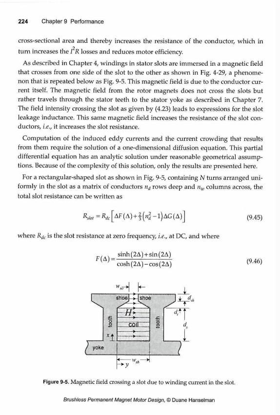
cross-sectional area and thereby increases the resistance of the conductor, which in turn increases the I R losses and reduces motor efficiency.

As described in Chapter 4, windings in stator slots are immersed in a magnetic field that crosses from one side of the slot to the other as shown in Fig. 4-29, a phenome-non that is repeated below as Fig. 9-5. This magnetic field is due to the conductor cur-rent itself. The magnetic field from the rotor magnets does not cross the slots but rather travels through the stator teeth to the stator yoke as described in Chapter 7. The field intensity crossing the slot as given by (4.23) leads to expressions for the slot leakage inductance. This same magnetic field increases the resistance of the slot con-ductors, i.e., it increases the slot resistance.

Computation of the induced eddy currents and the current crowding that results from them require the solution of a one-dimensional diffusion equation. This partial differential equation has an analytic solution under reasonable geometrical assump-tions. Because of the complexity of this solution, only the results are presented here.

For a rectangular-shaped slot as shown in Fig. 9-5, containing N turns arranged uni-formly in the slot as a matrix of conductors nj rows deep and nw columns across, the total slot resistance can be written as

¡Slot ~ R-dc AF(A) + f (« d 2 - l )AG(A)]

where R(/c is the slot resistance at zero frequency, i.e., at DC, and where

(9.45)

sinh ( 2 A ) + sin ( 2 A ) cosh (2A)-cos(2A) (9.46)

h

Figure 9-5. Magnetic field crossing a slot due to winding current in the slot.

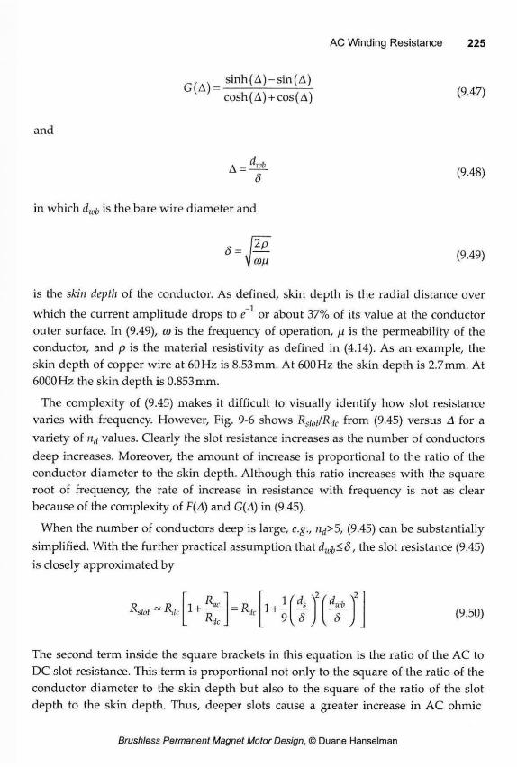
G(A) sinh(A)-sin(A) cosh (A) + cos (A) (9.47)

and

8 (9.48)

in which dwi, is the bare wire diameter and

(9.49)

is the skin depth of the conductor. As defined, skin depth is the radial distance over which the current amplitude drops to e 1 or about 37% of its value at the conductor outer surface. In (9.49), co is the frequency of operation, ¡J. is the permeability of the conductor, and p is the material resistivity as defined in (4.14). As an example, the skin depth of copper wire at 60Hz is 8.53mm. At 600Hz the skin depth is 2.7mm. At 6000Hz the skin depth is 0.853mm.

The complexity of (9.45) makes it difficult to visually identify how slot resistance varies with frequency. However, Fig. 9-6 shows Rsiot/R,k horn (9.45) versus A for a variety of nd values. Clearly the slot resistance increases as the number of conductors deep increases. Moreover, the amount of increase is proportional to the ratio of the conductor diameter to the skin depth. Although this ratio increases with the square root of frequency, the rate of increase in resistance with frequency is not as clear because of the complexity of F(A) and G(zi) in (9.45).

When the number of conductors deep is large, e.g., nd>5, (9.45) can be substantially simplified. With the further practical assumption that du,i,<8, the slot resistance (9.45) is closely approximated by

s/ol R. 'tic Rdc - R iic 9 8

\2 dwb 8

\2 (9.50)

The second term inside the square brackets in this equation is the ratio of the AC to DC slot resistance. This term is proportional not only to the square of the ratio of the conductor diameter to the skin depth but also to the square of the ratio of the slot depth to the skin depth. Thus, deeper slots cause a greater increase in AC ohmic

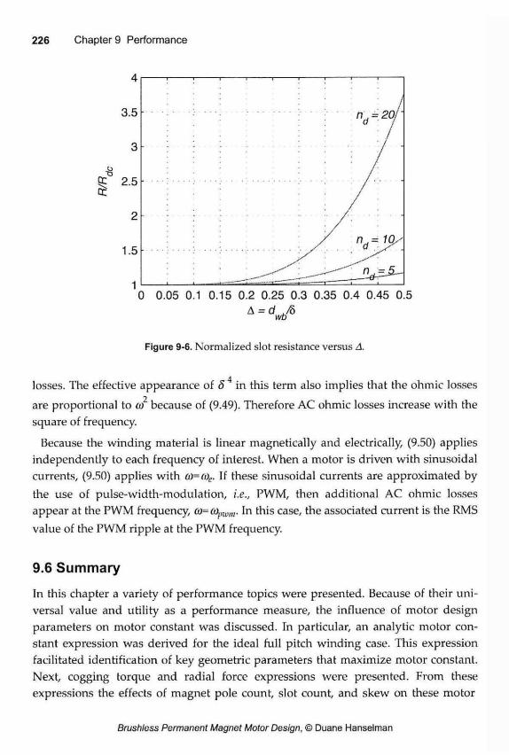
Figure 9-6. Normalized slot resistance versus A.

losses. The effective appearance of ¿T4 in this term also implies that the ohmic losses are proportional to co because of (9.49). Therefore AC ohmic losses increase with the square of frequency.

Because the winding material is linear magnetically and electrically (9.50) applies independently to each frequency of interest. When a motor is driven with sinusoidal currents, (9.50) applies with a>=a>e. If these sinusoidal currents are approximated by the use of pulse-width-modulation, i.e., PWM, then additional AC ohmic losses appear at the PWM frequency, £»= Cfyu„„. In this case, the associated current is the RMS value of the PWM ripple at the PWM frequency.

9.6 Summary

In this chapter a variety of performance topics were presented. Because of their uni-versal value and utility as a performance measure, the influence of motor design parameters on motor constant was discussed. In particular, an analytic motor con-stant expression was derived for the ideal full pitch winding case. This expression facilitated identification of key geometric parameters that maximize motor constant. Next, cogging torque and radial force expressions were presented. From these expressions the effects of magnet pole count, slot count, and skew on these motor

performance measures were identified. Because of their significant role in motor per-formance, a detailed discussion of core losses was presented. This discussion included identification of techniques to minimize them, difficulties in making accu-rate predictions of core losses, and presentation of one technique for estimating core losses from published core loss data. Lastly, expressions were presented that describe the increased winding resistance seen by currents at the fundamental electrical fre-quency and at PWM frequencies.

This chapter demonstrates the concepts presented in the preceding chapters by docu-menting example motor designs. The results presented here utilize the equations and procedures developed in the previous chapters. In addition, they rely on geometric calculations and material properties that were not presented.

Common Characteristics To facilitate comparisons among the designs, all motor designs share the following characteristics:

• The stator outside radius is Rso=50mm.

• The motor axial length is Ls/=100mm.

• The rotor outside radius Rm is chosen to maximize motor constant Km.

• The stator tooth body width wtb, stator yoke width wsy, and rotor yoke width wry are adjusted to keep the peak flux density in the regions close to 1.4T.

• No skewing of magnets or stator slots is employed.

• The ferromagnetic portions of the motor are constructed using common, high quality electrical steel.

• The radial magnet length is /„,=4mm and the air gap length is g=lmm.

• The magnets are radially magnetized and operate at Br=1.3T and /iR=1.05.

• The angular magnet pole width is set to 160°E, which gives a magnet frac-tion of am=160°E/180°E=0.89.

• The covered wire slot fill factor is set to kwc=60%.

• The phase currents are sinusoidal.

• The conductor current density is set to /=5Arms/mm .

• The windings operate at a temperature of 50°C.

• Windings are placed using the algorithm developed in Chapter 6.

The preceding common characteristics are not optimum for many designs but do reflect values typical to many designs. The parameters chosen promote comparison among motor designs by fixing important performance characteristics. For example, by setting the slot fill factor and conductor current density rather than the wire gage and conductor current, all motor designs have the same slot current density. So, while the total slot ampere-tums NI changes from design to design, the I R losses per unit slot volume are fixed. Because motor performance is fundamentally constrained by the ability to dissipate heat, fixing the I R losses per unit slot volume places all motor designs on a equal footing with respect to thermal capabilities.

Since motor constant Km describes the fundamental torque production efficiency of a motor, valid performance comparisons based on motor constant require that it be maximized with respect to motor volume. For this reason, the outside rotor radius of each design is chosen to maximize motor constant. As described in Chapter 9, motor constant is not a strong function of rotor outside radius when the motor outer diame-ter is fixed. As a result, while there is an optimum Rro, radii in the neighborhood of the optimum produce nearly the same motor constant.

The remainder of the parameters fix the motor magnetic operating point across all designs. While this condition does not fix the amount of permanent magnet material used, it fixes the contribution of the permanent magnets on motor performance.

While the presented designs focus on motor performance, they ignore cost. Though immensely important, the material and manufacturing cost of the designs cannot be compared using the information presented in this text. As a result, it is not possible to predict designs that maximize the ratio of performance to cost.

Presented Results Each motor design presented here utilizes two facing pages. The information con-tained on the facing pages includes:

• The table at the top of the left hand page identifies the number of magnet poles N„„ the number of stator slots Ns used in the design, and the number of slots per pole per phase Nspp=Ns/Nm/Nph.

• This table also contains important performance data. The ratio of the rotor outside radius to the stator outside radius RrofRso identifies the rotor radius that maximizes motor constant Km (4.40), which is given in N-m/VW. Though not used in the design computations, the minimum skew required to elimi-nate cogging torque (9.21) is given in terms of slot pitches. Finally, the first or fundamental harmonic index of the cogging torque nco„, given by

smallest value of n that satisfies (9.20), describes the relative harmonic fre-quency of the cogging torque.

• The middle of the left hand page shows a cross section of the motor design. This figure illustrates the relative dimensions of the design.

• The bottom of the left hand page contains motor winding information. The table shown identifies each coil in each phase. The coil angle describes the relative angle of each coil in a given phase. This information is used to com-pute the winding factor Kwn. As described in Chapter 6, for each phase, In and Out describes the slot number and direction for each coil making up each phase winding.

• Motor back EMFs are shown at the top of the right hand page. The figure depicts the phase back EMF e}lh(0) (6.11). In addition, the figure shows the line-to-line back EMF, which appears across two windings when the phases are connected in the Y-connection as shown in Fig. 8-6. In all designs, the back EMF amplitudes are normalized by the peak value of the line-to-line back EMF.

• The relative harmonic content of the phase back EMF eph(0) is shown in the middle of the right hand page. That is, the amplitude of the higher harmon-ics in epft(8) are shown relative to that of the fundamental component at har-monic index n=1. For example, if the third harmonic is shown at a level of 20%, then the third harmonic has an amplitude 20% of that of the funda-mental. This plot provides information about back EMF harmonic distor-tion.

• At the bottom of the right hand page, the amplitude of the winding factor Kwll (6.13) as a function of harmonic index is shown. This distribution describes how the harmonics of the coil back EMFs add when all coils are connected in series.

Notes • Not all valid combinations of magnet pole and slot counts are considered.

• Some performance data exhibits slight variability because the tooth body width and rotor and stator yoke widths have not been iteratively adjusted to produce identical magnetic circuit reluctance factors.

• The designs illustrated are simply that—illustrations. They may be good starting points for actual designs, but they are not necessarily optimal in any way.

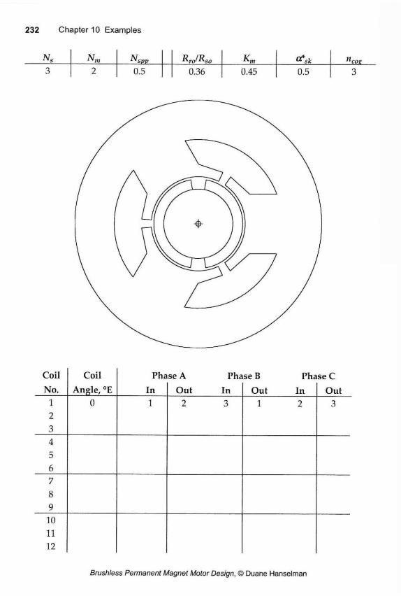
Ns Nm N RJRS0 <*sk ,lcos 3 2 0.5 0.36 0.45 0.5 3

Coil No.

Coil Angle, °E

Pha In

se A Pha Out In

se B Pha Out In

se C Out

1 2 3

0 1 2 3 1 2 3

4 5 6 7 8 9

10 11 12

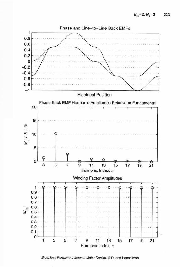
Electrical Position

Phase Back EMF Harmonie Amplitudes Relative to Fundamental

9 11 13 15 Harmonie Index, n

Winding Factor Amplitudes

7 9 11 13 15 17 19 21 Harmonie Index, n

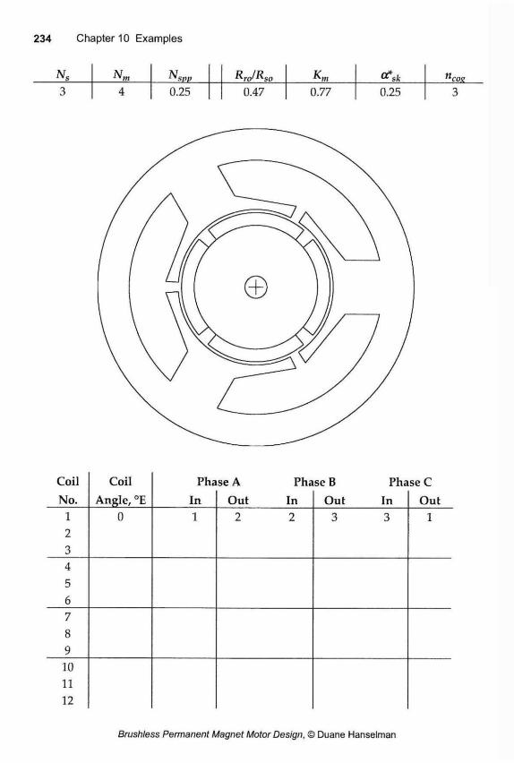
Ns Nm N R J R s o C?sk ncog 3 4 0.25 0.47 0.77 0.25 3

Coil No.

Coil Angle, °E

Pha In

se A Pha Out In

se B Pha Out In

se C Out

1 2 3

0 1 2 2 3 3 1

4 5 6 7 8 9 10 11 12

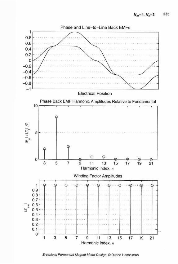
Phase Back EMF Harmonic Amplitudes Relative to Fundamental 10 I r-

9 11 13 15 Harmonic Index, n

Winding Factor Amplitudes

Electrical Position

—I— G)

—I— I 1 1 1 1 1 1 1 1— <p Q Q Q Q Q Q O Q

5 7 9 11 13 15 17 19 21 Harmonic Index, n

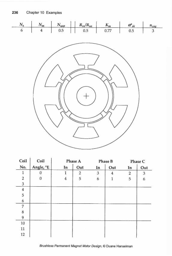
Ns N m Nsvp RJRso Km "roe 6 4 0.5 0.5 0.77 0.5 3

Coil No.

Coil Angle, °E

Pha In

se A Pha Out In

se B Pha Out In

seC Out

1 2 3

0 0

1 4

2 3 5 6

4 2 1 5

3 6

4 5 6 7 8 9 10 11 12

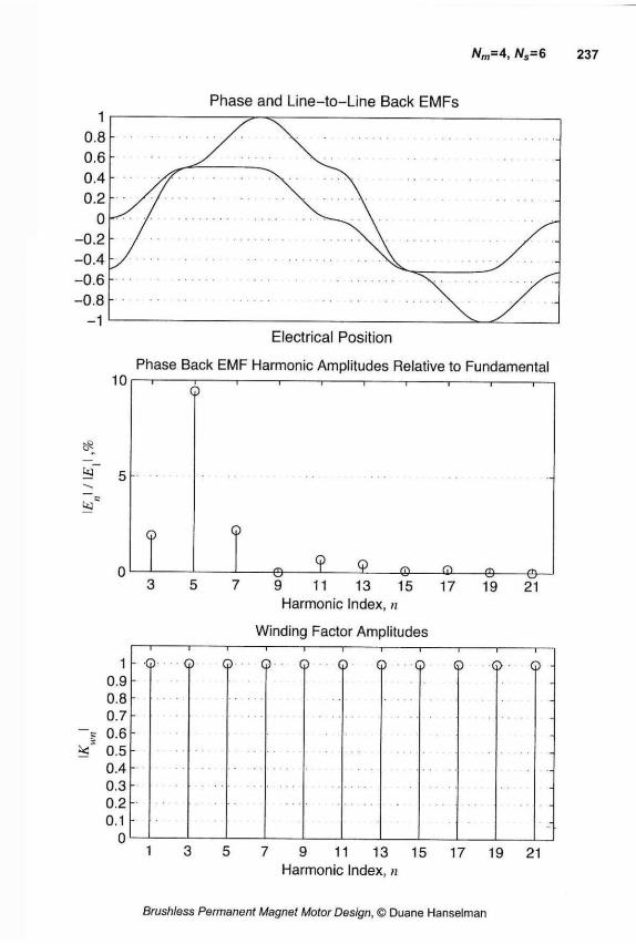
Electrical Position

Phase Back EMF Harmonic Amplitudes Relative to Fundamental

Q

-Q- - © -

9 11 13 15 17 19 21 Harmonic Index, n

Winding Factor Amplitudes

1 0.9 0.8 0.7 0.6 0.5 0.4 0.3 0.2 0.1

0

© G> O Q O O O O O Q

3 5 7 9 11 13 15 17 19 21 Harmonic Index, n

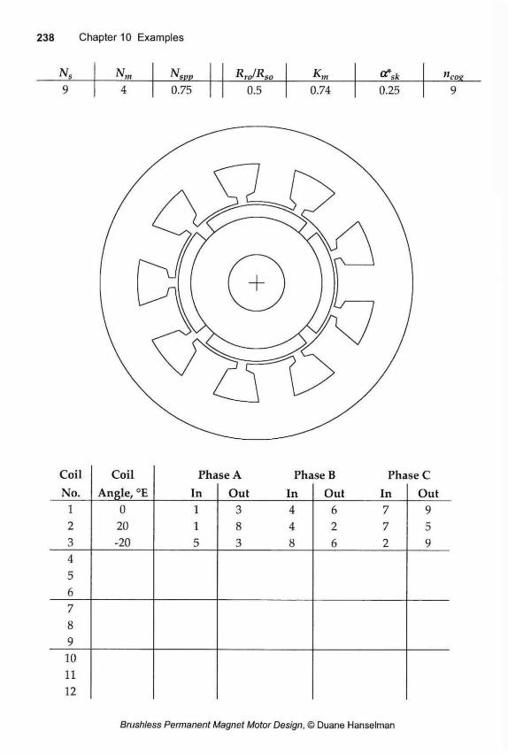
Ns Nm N sw

RJRso Km <x*sk Kcog 9 4 0.75 0.5 0.74 0.25 9

Coil No.

Coil Angle, °E

Pha In

se A Pha Out In

se B Pha Out In

seC Out

1 2 3

0 20 -20

1 1 5

3 4 8 4 3 8

6 7 2 7 6 2

9 5 9

4 5 6 7 8 9 10 11 12

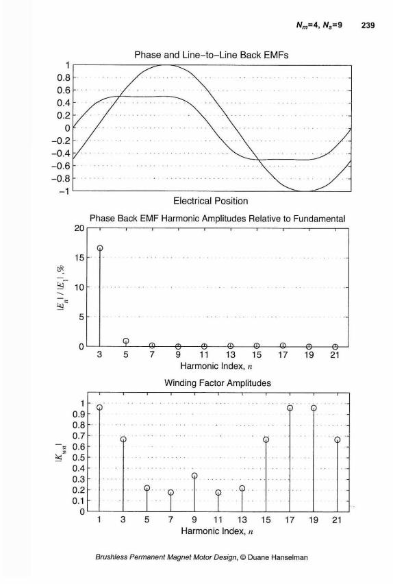
Nm=4, Ns=9

Electrical Position

Phase Back EMF Harmonic Amplitudes Relative to Fundamental

9 11 13 15 17 19 21 Harmonic Index, n

Winding Factor Amplitudes

1 0.9 0.8 0.7 0.6 0.5 0.4 0.3 0.2 0.1

0

-i 1 1 r Q Q Q

Q Ö

Q Q Q Q . .

Q

3 5 7 9 11 13 15 17 19 21 Harmonic Index, n

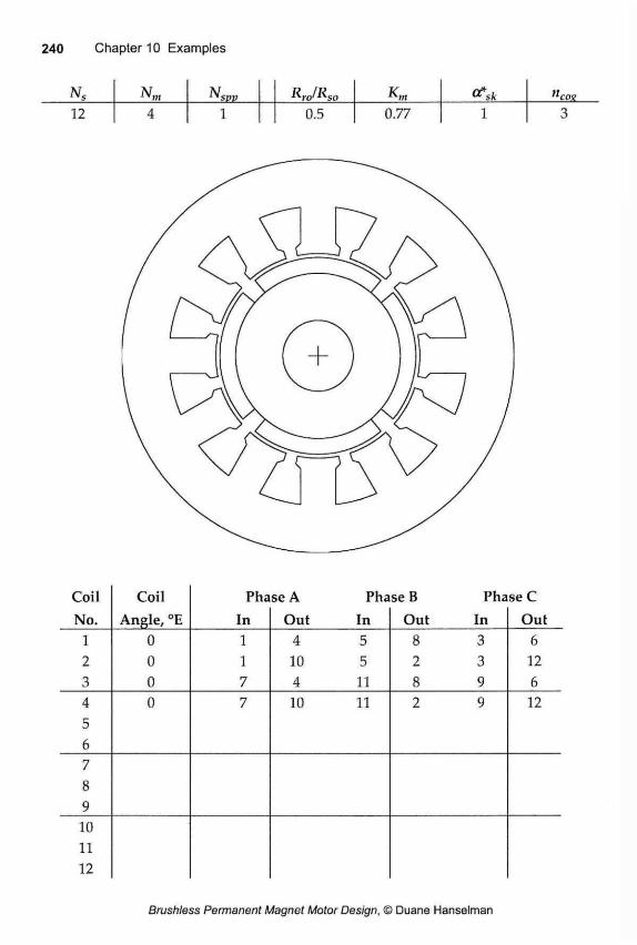
Ns Nm N RJRso Km <**sk "eoe 12 4 1 0.5 0.77 1 3

Coil Coil Phase A Phase B Phase C No. Angle, °E In Out In Out In Out

1 0 1 4 5 8 3 6 2 0 1 10 5 2 3 12 3 0 7 4 11 8 9 6 4 0 7 10 11 2 9 12 5 6 7 Q O 9 10 11 12

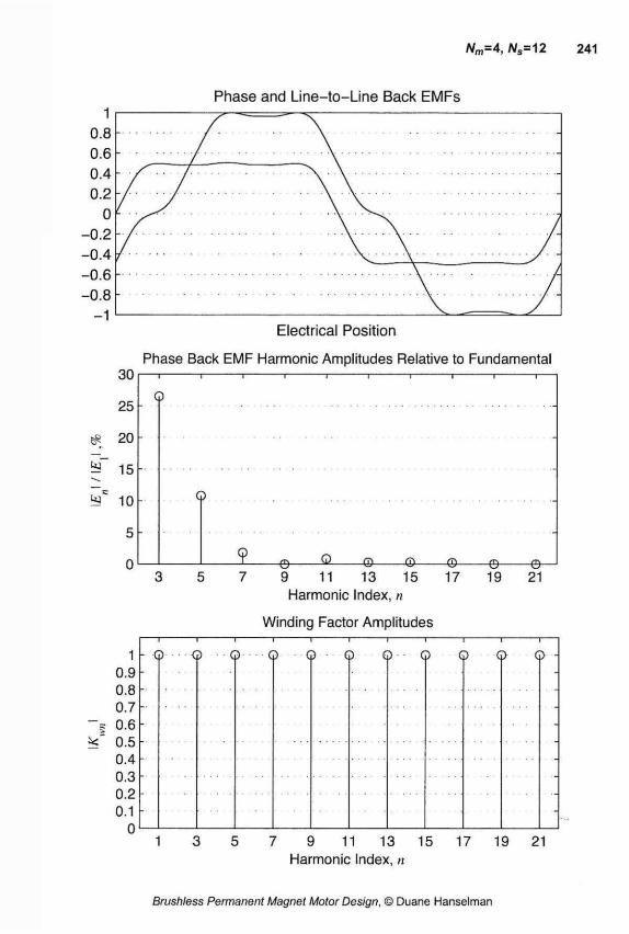
Nm=4, A/s=12 241

Electrical Position

Phase Back EMF Harmonic Amplitudes Relative to Fundamental

9 11 13 15 Harmonic Index, n

Winding Factor Amplitudes

7 9 11 13 15 17 Harmonic Index, n

19 21

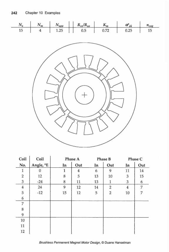
Nm N Rr0/Rs0 Km Mcog 15 4 1.25 0.5 0.72 0.25 15

Coil Coil Phase A Phase B Phase C No. Angle, °E In Out In Out In Out

1 0 1 4 6 9 11 14 2 12 8 5 13 10 3 15 3 -24 8 11 13 1 3 6 4 24 9 12 14 2 4 7 5 -12 15 12 5 2 10 7 6 7 Q O 9 10 11 12

Electrical Position

Phase Back EMF Harmonic Amplitudes Relative to Fundamental

7 9 11 13 15 Harmonic Index, n

Winding Factor Amplitudes

3 5 7 9 11 13 15 17 19 21 Harmonic Index, n

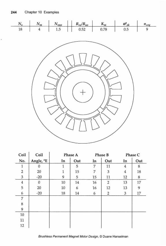
Ns N Rro/Rso Km "eoe 18 4 1.5 0.52 0.78 0.5 9

Coil Coil Phase A Phase B Phase C No. Angle, °E In Out In Out In Out

1 0 1 5 7 11 4 8 2 20 1 15 7 3 4 18 3 -20 9 5 15 11 12 8 4 0 10 14 16 2 13 17 5 20 10 6 16 12 13 9 6 -20 18 14 6 2 3 17 7 8 9 10 11 12

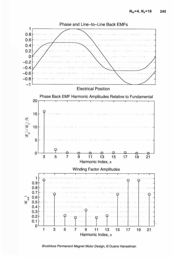
Electrical Position

Phase Back EMF Harmonic Amplitudes Relative to Fundamental 20 1 -i 1 1 1 1 1 1 r

7 9 11 13 15 17 19 21 Harmonic Index, n

Winding Factor Amplitudes

3 5 7 9 11 13 15 17 19 21 Harmonic Index, n

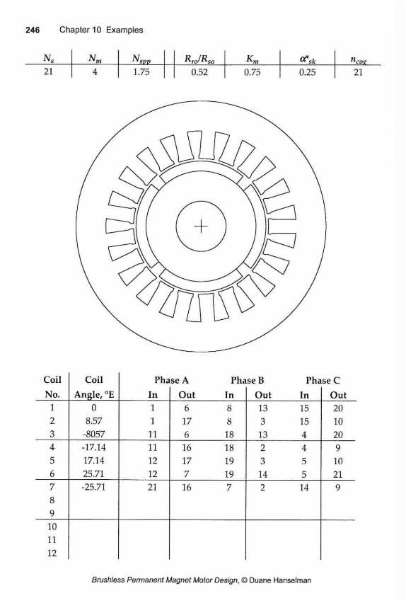
Ns N m N RJRso Km ncog 21 4 1.75 0.52 0.75 0.25 21

Coil Coil Phase A Phase B Phase C No. Angle, °E In Out In Out In Out

1 0 1 6 8 13 15 20 2 8.57 1 17 8 3 15 10 3 -8057 11 6 18 13 4 20 4 -17.14 11 16 18 2 4 9 5 17.14 12 17 19 3 5 10 6 25.71 12 7 19 14 5 21 7 Q

-25.71 21 16 7 2 14 9

9 10 11 12

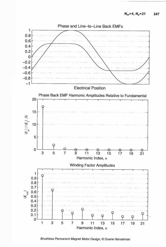
Electrical Position

Phase Back EMF Harmonie Amplitudes Relative to Fundamental

7 9 11 13 15 Harmonie Index, n

Winding Factor Amplitudes

7 9 11 13 15 17 19 21 Harmonie Index, n

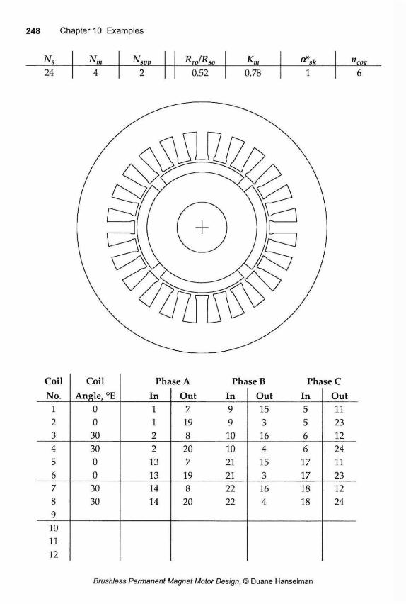
Ns Nm ^SPP RJRso Km ncog 24 4 2 0.52 0.78 1 6

Coil Coil Phase A Phase B Phase C No. Angle, °E In Out In Out In Out

1 0 1 7 9 15 5 11 2 0 1 19 9 3 5 23 3 30 2 8 10 16 6 12 4 30 2 20 10 4 6 24 5 0 13 7 21 15 17 11 6 0 13 19 21 3 17 23 7 30 14 8 22 16 18 12 8 30 14 20 22 4 18 24 9 10 11 12

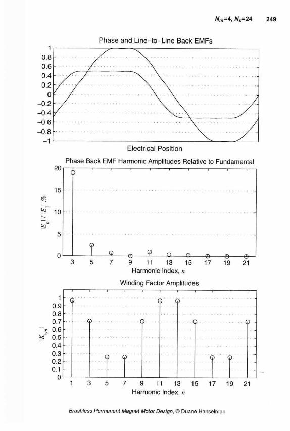
Electrical Position

Phase Back EMF Harmonic Amplitudes Relative to Fundamental

1 0.9 0.8 0.7 0.6 0.5 0.4 0.3 0.2 0.1

0

Q

7 9 11 13 15 Harmonic Index, n

Winding Factor Amplitudes —I r Q O

Q Q

Q Q

Q Q -

Q O

3 5 7 9 11 13 15 17 19 21 Harmonic Index, n

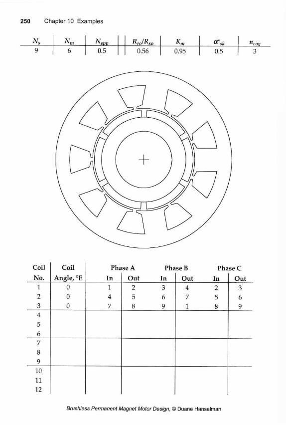
Ns Nm RJRso Km a*s k ncox 9 6 0.5 0.56 0.95 0.5 3

Coil No.

Coil Angle, °E

Pha In

se A Pha Out In

se B Pha Out In

se C Out

1 2 3

0 0 0

1 4 7

2 3 5 6 8 9

4 2 7 5 1 8

3 6 9

4 5 6 7 8 9 10 11 12

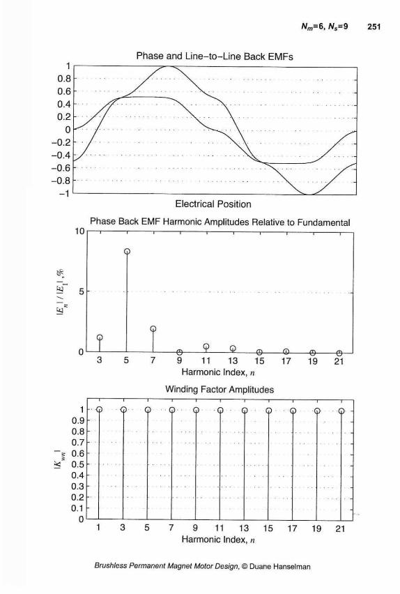
A/m=6, Ns=9

1 0.9 0.8 0.7 0.6 0.5 0.4 0.3 0.2 0.1

0

Electrical Position

Phase Back EMF Harmonic Amplitudes Relative to Fundamental

9 11 13 15 Harmonic Index, n

Winding Factor Amplitudes

<P —I— <2) Q- Q

—I— Q O Q Q ~i—

7 9 11 13 15 Harmonic Index, n

17 19 21

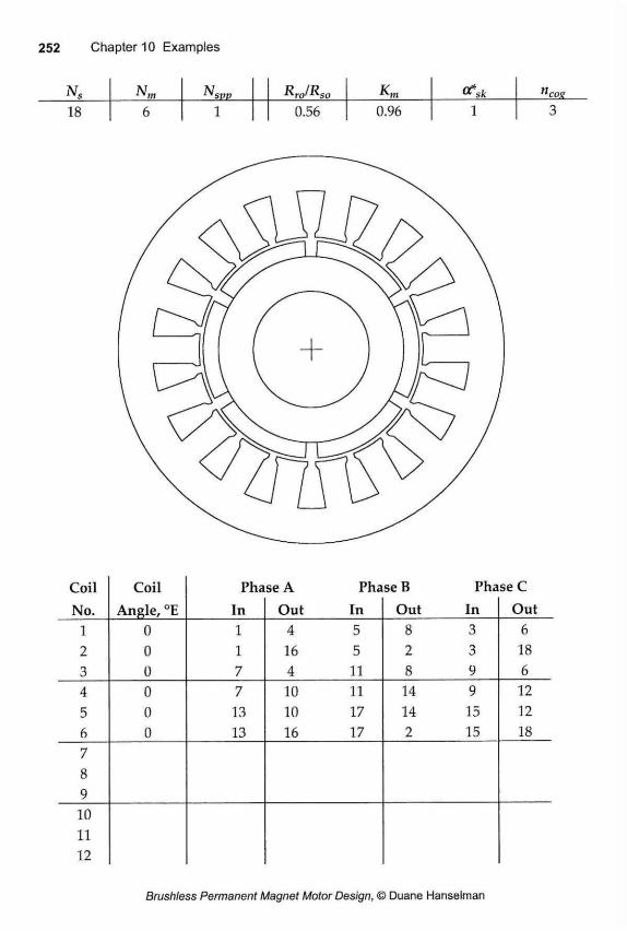
Ns Nspp RJRso Kn Ofsk ttcog 18 6 1 0.56 0.96 1 3

Coil Coil Phase A Phase B Phase C No. Angle, °E In Out In Out In Out

1 0 1 4 5 8 3 6 2 0 1 16 5 2 3 18 3 0 7 4 11 8 9 6 4 0 7 10 11 14 9 12 5 0 13 10 17 14 15 12 6 0 13 16 17 2 15 18 7 8 9 10 11 12

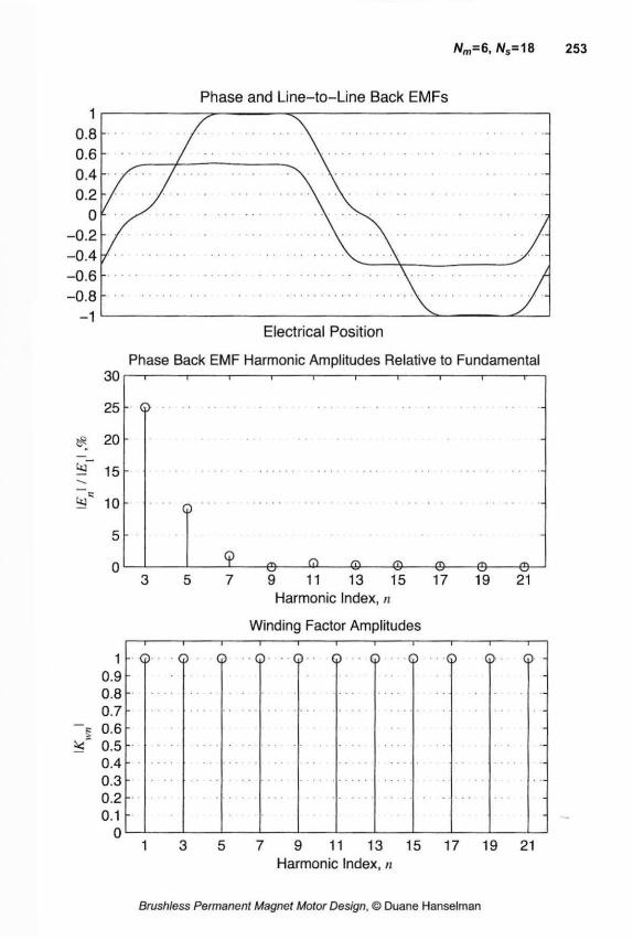
Nm-G, Ns=18 253

3 5 7 9 11 13 15 17 19 21 Harmonic Index, n

Electrical Position

Phase Back EMF Harmonic Amplitudes Relative to Fundamental 30 I—r

- e — 9 11 13 15

Harmonic Index, n

Winding Factor Amplitudes

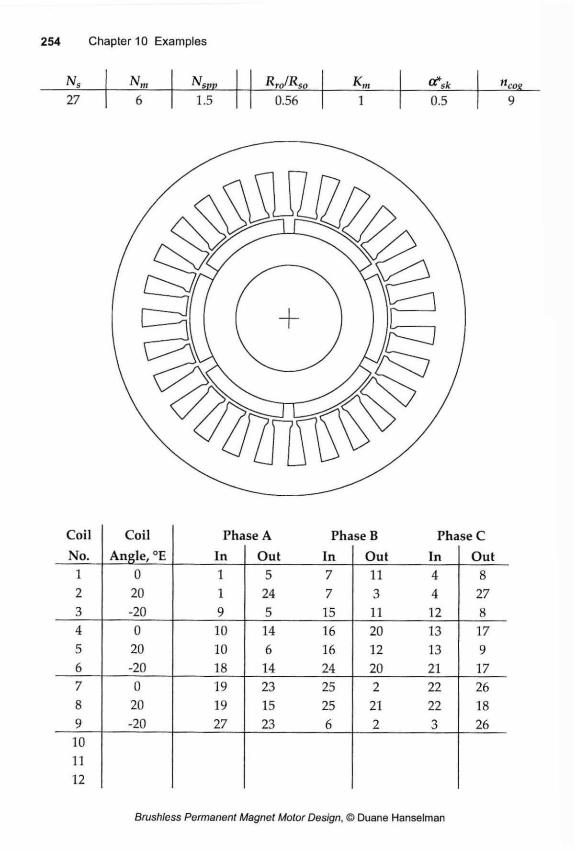
Ns N m N svv RJRS0 ncos 27 6 1.5 0.56 1 0.5 9

Coil Coil Phase A Phase B Phase C No. Angle, °E In Out In Out In Out

1 0 1 5 7 11 4 8 2 20 1 24 7 3 4 27 3 -20 9 5 15 11 12 8 4 0 10 14 16 20 13 17 5 20 10 6 16 12 13 9 6 -20 18 14 24 20 21 17 7 0 19 23 25 2 22 26 8 20 19 15 25 21 22 18 9 -20 27 23 6 2 3 26 10 11 12

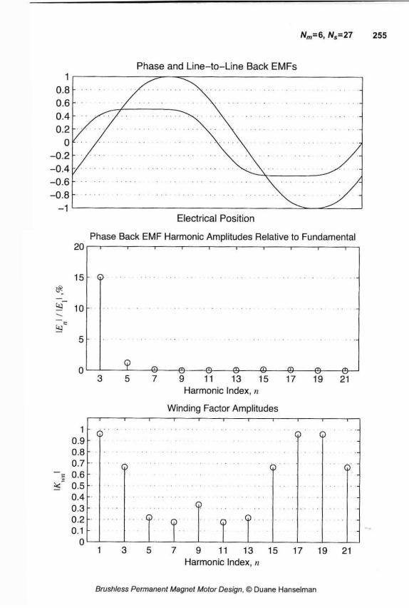
A/m=6, Ns=27 255

Electrical Position

Phase Back EMF Harmonie Amplitudes Relative to Fundamental 20 —i 1 1 1 1 1 r r-

7 9 11 13 15 Harmonie Index, n

Winding Factor Amplitudes

1 0.9 0.8 0.7 0.6 0.5 0.4 0.3 0.2 0.1

0

Q o 9

9

9

3 5 7 9 11 13 15 17 19 21 Harmonie Index, n

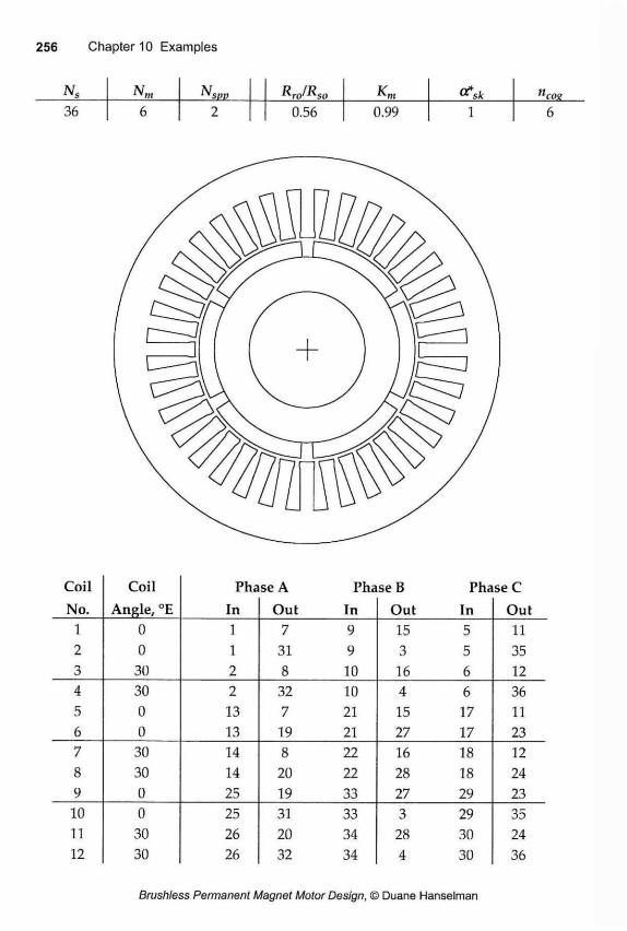
Nm Ns„0 RJRS0 Km 0*s k "roe 36 6 2 0.56 0.99 1 6

Coil Coil Phase A Phase B Phase C No. Angle, °E In Out In Out In Out

1 0 1 7 9 15 5 11 2 0 1 31 9 3 5 35 3 30 2 8 10 16 6 12 4 30 2 32 10 4 6 36 5 0 13 7 21 15 17 11 6 0 13 19 21 27 17 23 7 30 14 8 22 16 18 12 8 30 14 20 22 28 18 24 9 0 25 19 33 27 29 23 10 0 25 31 33 3 29 35 11 30 26 20 34 28 30 24 12 30 26 32 34 4 30 36

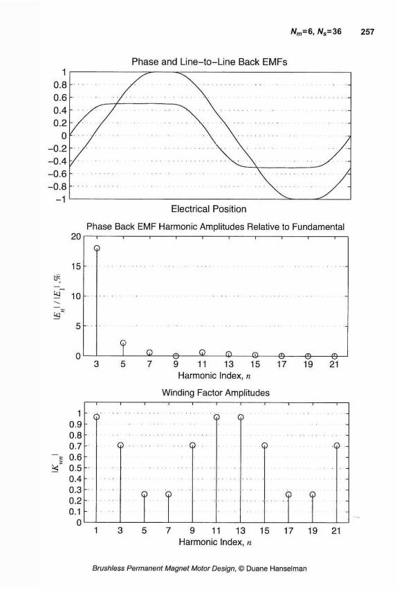
Electrical Position

Phase Back EMF Harmonie Amplitudes Relative to Fundamental

7 9 11 13 15 Harmonie Index, n

Winding Factor Amplitudes

1 0.9 0.8 0.7 0.6 0.5 0.4 0.3 0.2 0.1

0

Q Q Q

9 Q

Q Q

Q © -

Q G)

1 3 5 7 9 11 13 15 17 19 21 Harmonie Index, n

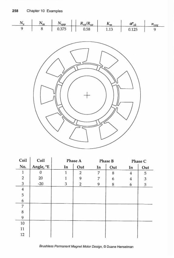
Nm N RJRS0 Km "cos 9 8 0.375 0.58 1.13 0.125 9

Coil No.

Coil Angle, °E

Pha In

se A Pha Out In

ise B Pha Out In

seC Out

1 2 3

0 20 -20

1 1 3

2 7 9 7 2 9

8 4 6 4 8 6

5 3 5

4 5 6 7 8 9 10 11 12

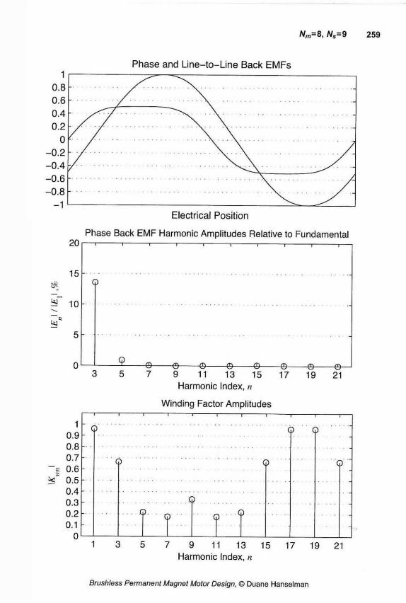
Electrical Position

Phase Back EMF Harmonic Amplitudes Relative to Fundamental

7 9 11 13 15 Harmonic Index, n

Winding Factor Amplitudes

19 21

1 0.9 0.8 0.7 0.6 0.5 0.4 0.3 0.2 0.1

0

0 Q O

0

0 0 Q Q

0

Q

0

7 9 11 13 15 17 19 21 Harmonic Index, n

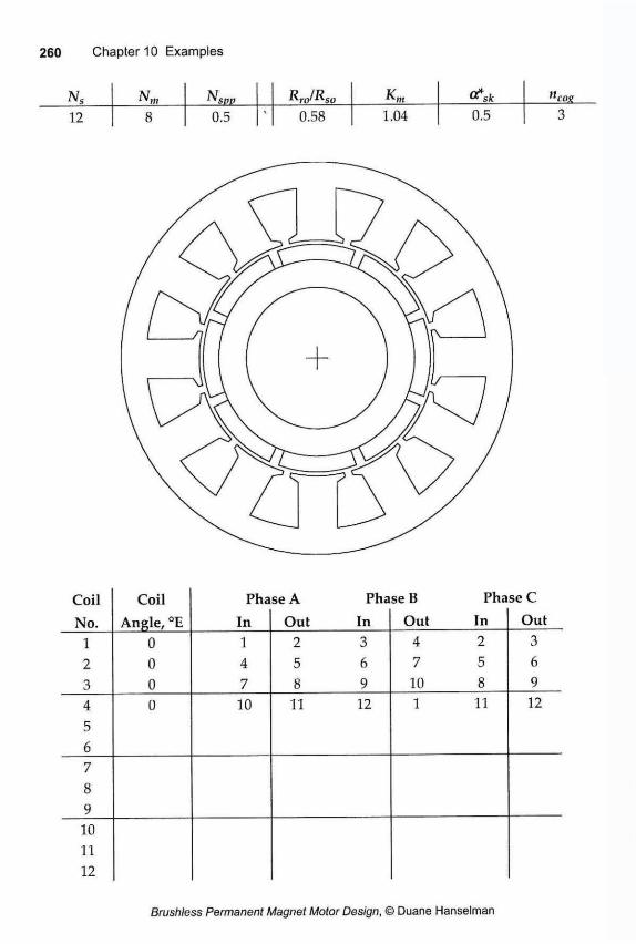
Ns Nm N Rro/Rso Km s k "eoe 12 8 0.5 » 0.58 1.04 0.5 3

Coil Coil Phase A Phase B Phase C

No. Angle, °E In Out In Out In Out 1 0 1 2 3 4 2 3 2 0 4 5 6 7 5 6 3 0 7 8 9 10 8 9 4 0 10 11 12 1 11 12 5 6 7

O 9 10 11 12

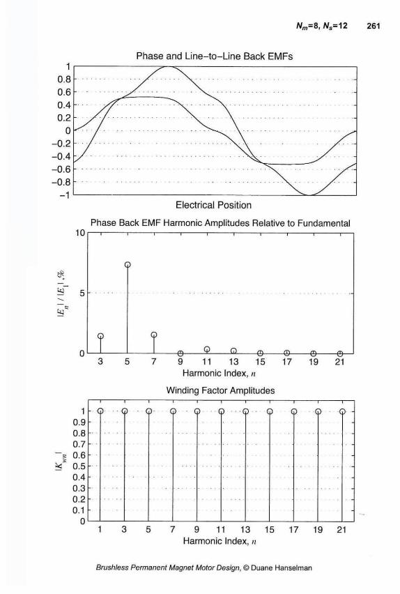
Phase Back EMF Harmonic Amplitudes Relative to Fundamental

7 9 11 13 15 Harmonic Index, n

Winding Factor Amplitudes

Electrical Position

•Q —I— O Q G) Q Q Q Q Q G> Q -

7 9 11 13 15 Harmonic Index, n

17 19 21

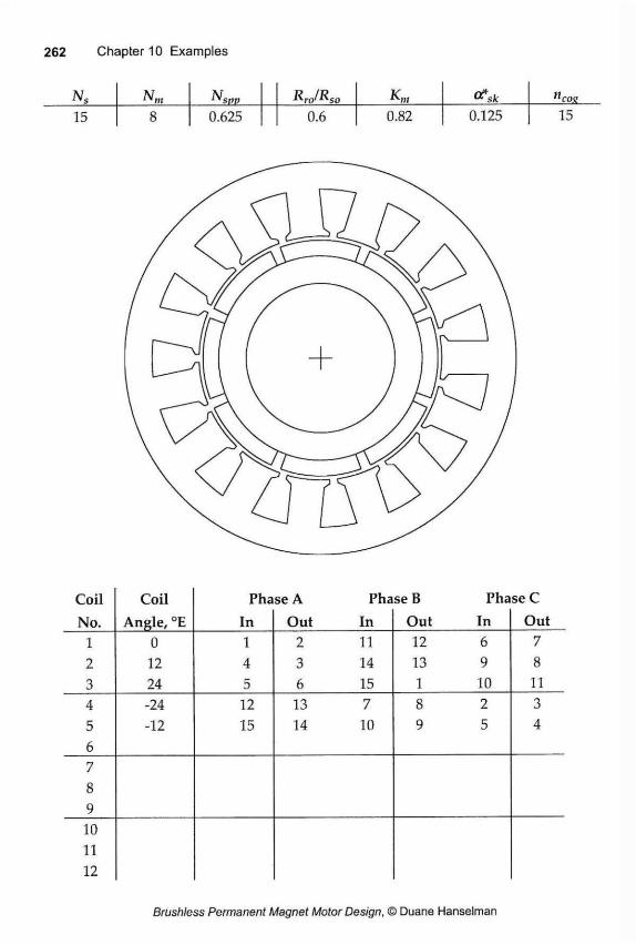
Ns Nm pp RjRso Kn cfsk ncos 15 8 0.625 0.6 0.82 0.125 15

Coil Coil Phase A Phase B Phase C No. Angle, °E In Out In Out In Out

1 0 1 2 11 12 6 7 2 12 4 3 14 13 9 8 3 24 5 6 15 1 10 11 4 -24 12 13 7 8 2 3 5 -12 15 14 10 9 5 4 6 7 8 9 10 11 12

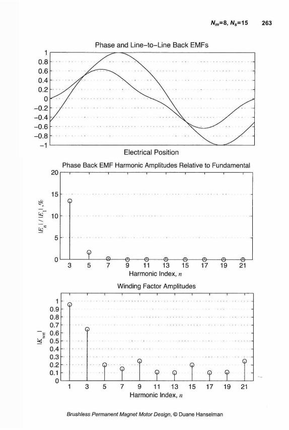
Electrical Position

Phase Back EMF Harmonic Amplitudes Relative to Fundamental

7 9 11 13 15 Harmonic Index, n

Winding Factor Amplitudes

1 0.9 0.8 0.7 0.6 0.5 0.4 0.3 0.2 0.1

0

Q

Q

© © Q Q ©

? ? I ? ? 7 9 11 13 15 17 19 21

Harmonic Index, n

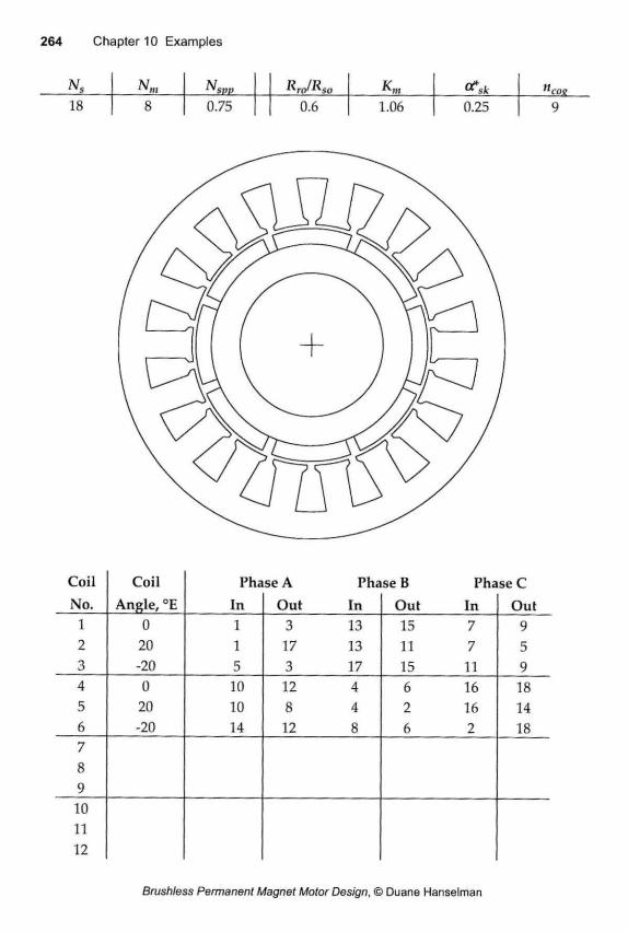
Ns Nm N RJRso <?sk "eoe 18 8 0.75 0.6 1.06 0.25 9

Coil Coil Phase A Phase B Phase C No. Angle, °E In Out In Out In Out

1 0 1 3 13 15 7 9 2 20 1 17 13 11 7 5 3 -20 5 3 17 15 11 9 4 0 10 12 4 6 16 18 5 20 10 8 4 2 16 14 6 -20 14 12 8 6 2 18 7 Q O 9 10 11 12

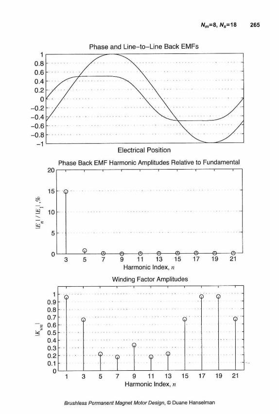
Nm=8, A/s=18

Electrical Position

Phase Back EMF Harmonic Amplitudes Relative to Fundamental

7 9 11 13 15 Harmonic Index, n

Winding Factor Amplitudes

3 5 7 9 11 13 15 17 19 21 Harmonic Index, n

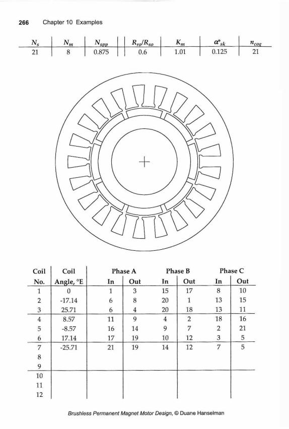
N m RJRS0 Kn "eoe 21 8 0.875 0.6 1.01 0.125 21

Coil Coil Phase A Phase B Phase C No. Angle, °E In Out In Out In Out

1 0 1 3 15 17 8 10 2 -17.14 6 8 20 1 13 15 3 25.71 6 4 20 18 13 11 4 8.57 11 9 4 2 18 16 5 -8.57 16 14 9 7 2 21 6 17.14 17 19 10 12 3 5 7 -25.71 21 19 14 12 7 5 8 9 10 11 12

10

Ï" 5

Electrical Position

Phase Back EMF Harmonie Amplitudes Relative to Fundamental

Q

1 . 7 9 11 13 15

Harmonie Index, n

Winding Factor Amplitudes

17 19 21

7 9 11 13 15 17 Harmonie Index, n

19 21

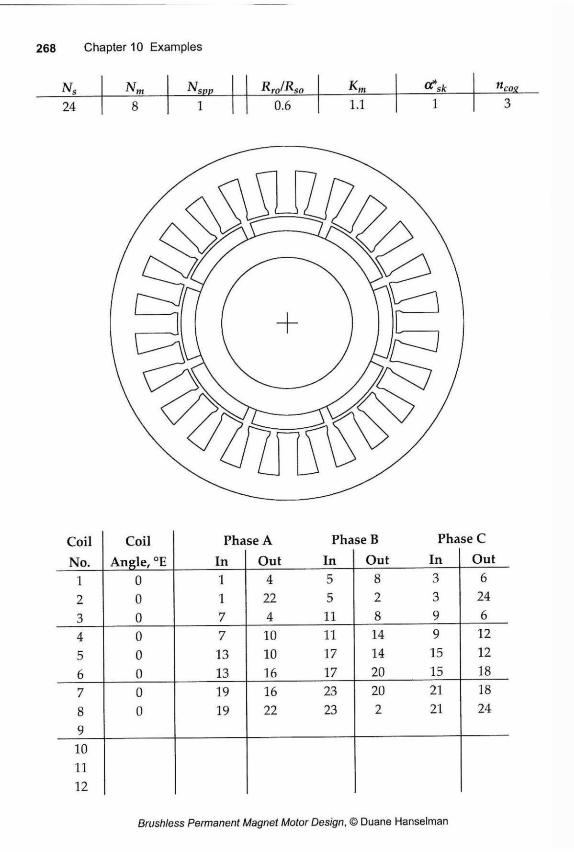
Ns Nm N RJRso Km ncux 24 8 1 0.6 1.1 1 3

Coil Coil Phase A Phase B Phase C

No. Angle, °E In Out In Out In Out 1 0 1 4 5 8 3 6 2 0 1 22 5 2 3 24 3 0 7 4 11 8 9 6 4 0 7 10 11 14 9 12 5 0 13 10 17 14 15 12 6 0 13 16 17 20 15 18 7 0 19 16 23 20 21 18 8 0 19 22 23 2 21 24 9 10 11 12

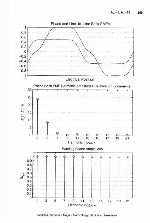
A/m=8, Ns=24

Electrical Position

Phase Back EMF Harmonic Amplitudes Relative to Fundamental

9 11 13 15 17 19 21 Harmonic Index, n

Winding Factor Amplitudes

1 0.9 0.8 0.7 0.6 0.5 0.4 0.3 0.2 0.1

0

- ©

n r-<3 © © © © © © © © -

3 5 7 9 11 13 15 17 19 21 Harmonic Index, n

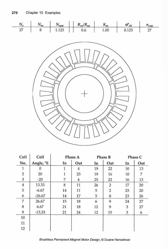
Nm Nsvv RJRso a*sfc 1 1 cos 27 8 1.125 0.6 1.05 0.125 27

Coil Coil Phase A Phase B Phase C No. Angle, °E In Out In Out In Out

1 0 1 4 19 22 10 13 2 20 1 25 19 16 10 7 3 -20 7 4 25 22 16 13 4 13.33 8 11 26 2 17 20 5 -6.67 14 11 5 2 23 20 6 -26.67 14 17 5 8 23 26 7 26.67 15 18 6 9 24 27 8 6.67 21 18 12 9 3 27 9 -13.33 21 24 12 15 3 6 10 11 12

A/m=8, Ns=27

Electrical Position

Phase Back EMF Harmonic Amplitudes Relative to Fundamental

9 11 13 15 Harmonic Index, n

Winding Factor Amplitudes

7 9 11 13 15 17 19 21 Harmonic Index, n

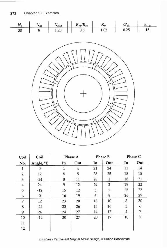
Ns Nm N RJRso ncos 30 8 1.25 0.6 1.02 0.25 15

Coil Coil Phase A Phase B Phase C

No. Angle, °E In Out In Out In Out 1 0 1 4 21 24 11 14 2 12 8 5 28 25 18 15 3 -24 8 11 28 1 18 21 4 24 9 12 29 2 19 22 5 -12 15 12 5 2 25 22 6 0 16 19 6 9 26 29 7 12 23 20 13 10 3 30 8 -24 23 26 13 16 3 6 9 24 24 27 14 17 4 7 10 -12 30 27 20 17 10 7 11 12

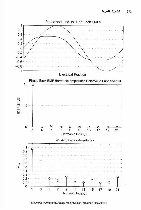
Nm=8, Ns=30 273

Electrical Position

Phase Back EMF Harmonic Amplitudes Relative to Fundamental

9 11 13 15 17 19 21 Harmonic Index, n

Winding Factor Amplitudes

3 5 7 9 11 13 15 17 19 21 Harmonic Index, n

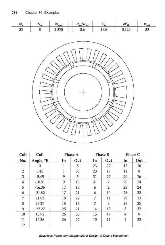
N m N RJRso "cos 33 8 1.375 0.6 1.06 0.125 33

Coil Coil Phase A Phase B Phase C No. Angle, °E In Out In Out In Out

1 0 1 5 23 27 12 16 2 5.45 1 30 23 19 12 8 3 -5.45 9 5 31 27 20 16 4 -10.91 9 13 31 2 20 24 5 -16.36 17 13 6 2 28 24 6 -21.82 17 21 6 10 28 32 7 21.82 18 22 7 11 29 33 8 27.27 18 14 7 3 29 25 9 -27.27 25 21 14 10 3 32 10 10.91 26 30 15 19 4 8 11 16.36 26 22 15 11 4 33 12

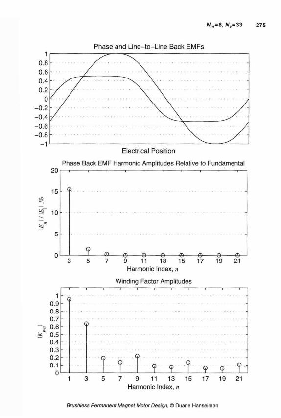
Nm=8, Ns=33 275

7 9 11 13 15 17 19 21 Harmonic Index, n

C7 o O o o 7 9 11 13 15 17 19 21

Harmonic Index, n Winding Factor Amplitudes

Phase Back EMF Harmonic Amplitudes Relative to Fundamental 201

Electrical Position

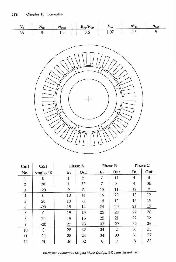
Ns N m N Rro/Rso "coy 36 8 1.5 0.6 1.0 7 0.5 9

Coil Coil Phase A Phase B Phase C

No. Angle, °E In Out In Out In Out 1 0 1 5 7 11 4 8 2 20 1 33 7 3 4 36 3 -20 9 5 15 11 12 8 4 0 10 14 16 20 13 17 5 20 10 6 16 12 13 19 6 -20 18 14 24 20 21 17 7 0 19 23 25 29 22 26 8 20 19 15 25 21 22 18 9 -20 27 23 33 29 30 26 10 0 28 32 34 2 31 35 11 20 28 24 34 30 31 27 12 -20 36 32 6 2 3 35

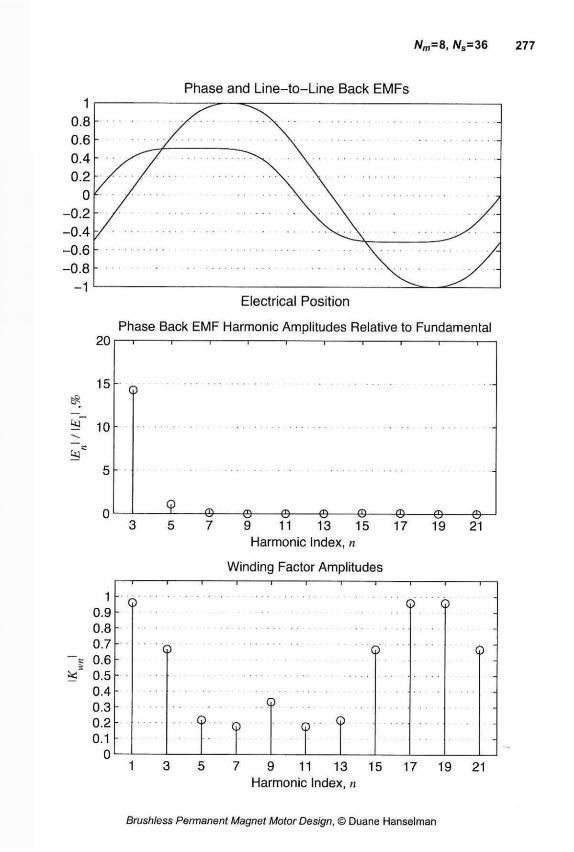
Nm=8, A/s=36 277

1 0.8 0.6 0.4 0.2

0 - 0 . 2

-0 .4 - 0 . 6 - 0 . 8

- 1

Electrical Position

Phase Back EMF Harmonic Amplitudes Relative to Fundamental 20

15

iS 10

0 3 5 7 9 11 13 15 17 19 21

Harmonic Index, n Winding Factor Amplitudes

1 0.9 0 . 8 0.7 0.6 0.5 0.4 0.3 0.2 0.1

0

Q

- © © © © © © © © -

I I I ~i 1 1 1 r Q Q Q

© Q Q

. Q Q. © Q Q

1 3 5 7 9 11 13 15 17 19 21 Harmonic Index, n

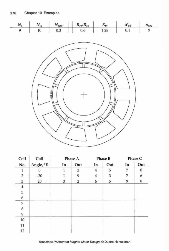
Nm N RJRso "cos 9 10 0.3 0.6 1.28 0.1 9

Coil No.

Coil Angle, °E

Pha In

se A Pha Out In

se B Pha Out In

seC Out

1 2 3

0 -20 20

1 1 3

2 4 9 4 2 6

5 7 3 7 5 9

8 6 8

4 5 6 7 8 9 10 11 12

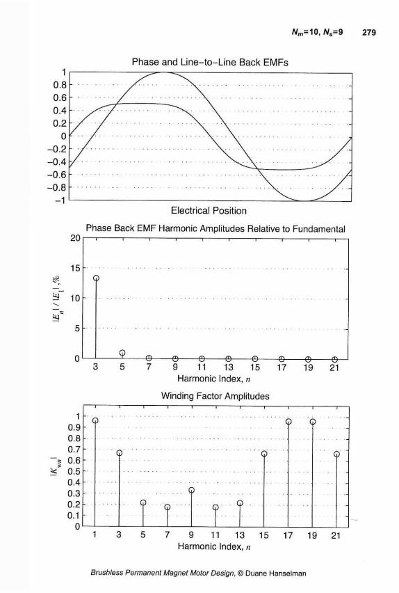
Electrical Position

Phase Back EMF Harmonic Amplitudes Relative to Fundamental

9 11 13 15 Harmonic Index, n

Winding Factor Amplitudes

3 5 7 9 11 13 15 17 19 21 Harmonic Index, n

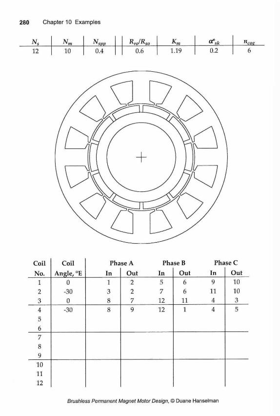
Ns Nm N Rro/Rso Km o*sfc ncos 12 10 0.4 0.6 1.19 0.2 6

Coil Coil Phase A Phase B Phase C No. Angle, °E In Out In Out In Out

1 0 1 2 5 6 9 10 2 -30 3 2 7 6 11 10 3 0 8 7 12 11 4 3 4 -30 8 9 12 1 4 5 5 6 7 8 9

10 11 12

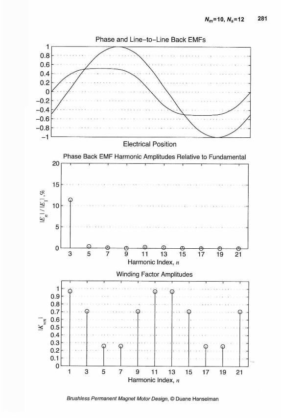
Nm=10,Ws=12 281

Electrical Position

Phase Back EMF Harmonie Amplitudes Relative to Fundamental

1 0.9 0.8 0.7 0.6 0.5 0.4 0.3 0.2 0.1

0

0

7 9 11 13 15 Harmonie Index, n

Winding Factor Amplitudes —i 1— © ©

© ©

Q Q

© ©

© ©

3 5 7 9 11 13 15 17 19 21 Harmonie Index, n

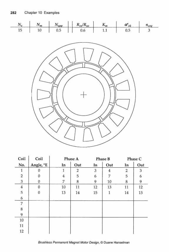
Ns Nm N svv

RJRso K>n 0<*sk 1 1 cox 15 10 0.5 0.6 1.1 0.5 3

Coil Coil Phase A Phase B Phase C No. Angle, °E In Out In Out In Out

1 0 1 2 3 4 2 3 2 0 4 5 6 7 5 6 3 0 7 8 9 10 8 9 4 0 10 11 12 13 11 12 5 0 13 14 15 1 14 15 6 7

O 9 10 11 12

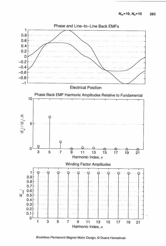
A/m=10, A/s=15 283

1 0.8 0.6 0.4 0.2

0 - 0 . 2

- 0 . 4 - 0 . 6

- 0 . 8

- 1

Electrical Position

Phase Back EMF Harmonic Amplitudes Relative to Fundamental 10

a" 5

Harmonic Index, n

Winding Factor Amplitudes

1 0.9 0.8 0.7 0.6

ÉS' 0.5 0.4 0.3 0.2 0.1

0

1 1 1 r ~~l 1 1 r-

©

Q -© ® Q q ©_ -e ©-

3 5 7 9 11 13 15 17 19 21

I r~ 9 9 9 0 0 © © © 9 © Q .

1 3 5 7 9 11 13 15 17 19 21 Harmonic Index, n

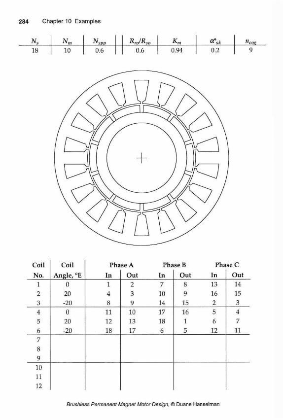
Ns Kn Nsvp R r o/R s o 0?sk "cos 18 10 0.6 0.6 0.94 0.2 9

Coil Coil Phase A Phase B Phase C No. Angle, °E In Out In Out In Out

1 0 1 2 7 8 13 14 2 20 4 3 10 9 16 15 3 -20 8 9 14 15 2 3 4 0 11 10 17 16 5 4 5 20 12 13 18 1 6 7 6 -20 18 17 6 5 12 11 7

O 9 10 11 12

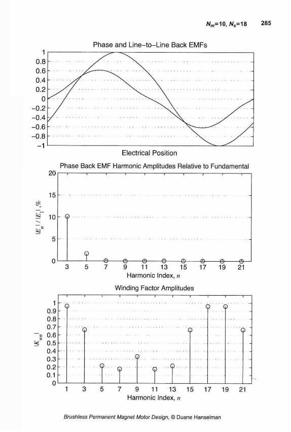
A/m=10, Ws=18 285

Electrical Position

Phase Back EMF Harmonie Amplitudes Relative to Fundamental

7 9 11 13 15 Harmonie Index, n

Winding Factor Amplitudes

1 0.9 0.8 0.7 0.6 0.5 0.4 0.3 0.2 0.1

0

Q

Q

Q Q

Q

Q. Q Q . Q

Q

7 9 11 13 15 17 19 21 Harmonie Index, n

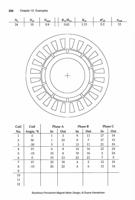
Ns N RJRS0 Km ncos 24 10 0.8 0.62 1.13 0.2 12

Coil Coil Phase A Phase B Phase C No. Angle, °E In Out In Out In Out

1 0 1 3 9 11 17 19 2 30 1 23 9 7 17 15 3 -30 5 3 13 11 21 19 4 15 6 8 14 16 22 24 5 -15 10 8 18 16 2 24 6 0 15 13 23 21 7 5 7 15 20 18 4 2 12 10 8 -15 20 22 4 6 12 14 9 10 11 12

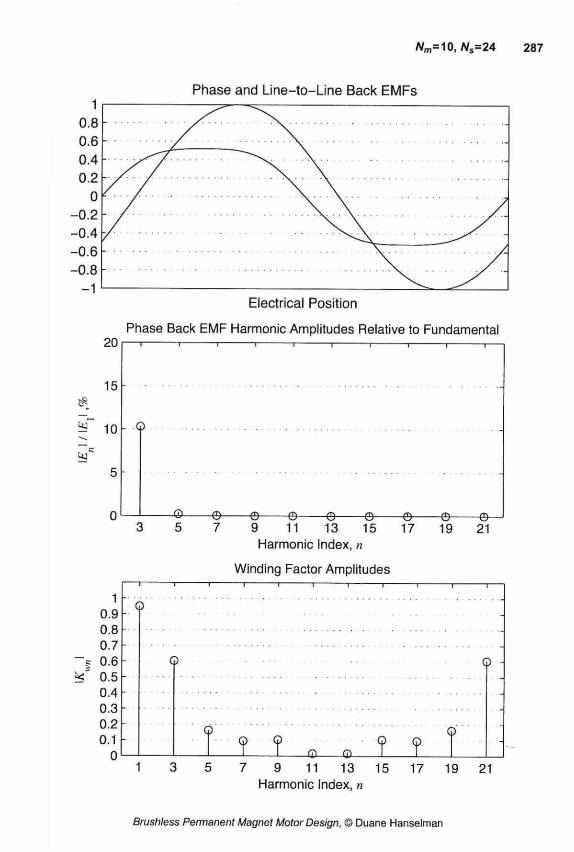
N„=10, =24 287

Electrical Position

Phase Back EMF Harmonic Amplitudes Relative to Fundamental

9 11 13 15 Harmonic Index, n

Winding Factor Amplitudes

7 9 11 13 15 17 19 21 Harmonic Index, n

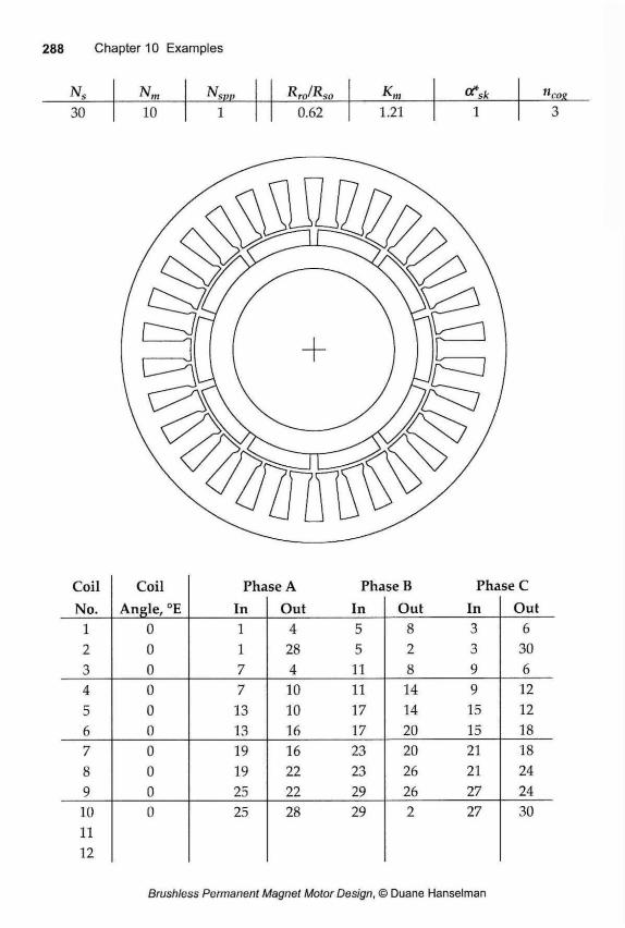
Ns Nm N Rro/Rso Km "cos 30 10 1 0.62 1.21 1 3

Coil Coil Phase A Phase B Phase C No. Angle, °E In Out In Out In Out

1 0 1 4 5 8 3 6 2 0 1 28 5 2 3 30 3 0 7 4 11 8 9 6 4 0 7 10 11 14 9 12 5 0 13 10 17 14 15 12 6 0 13 16 17 20 15 18 7 0 19 16 23 20 21 18 8 0 19 22 23 26 21 24 9 0 25 22 29 26 27 24 10 0 25 28 29 2 27 30 11 12

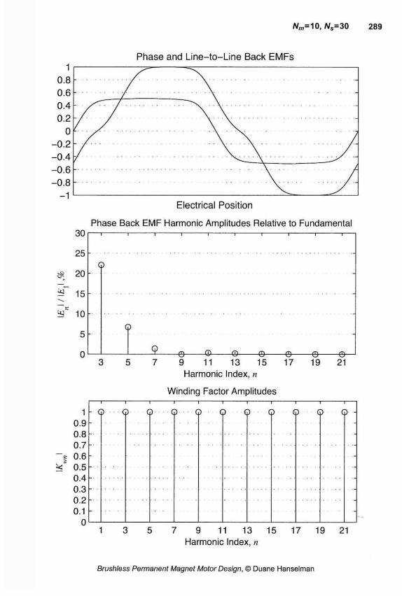
A/m=10, Ns= 30 289

Electrical Position

Phase Back EMF Harmonic Amplitudes Relative to Fundamental

©1 fcf

1 0.9 0.8 0.7 0.6 0.5 0.4 0.3 0.2 0.1

0

- Q —I— ©

7 9 11 13 15 Harmonic Index, n

Winding Factor Amplitudes i 1 1 1 1 1—

Q Q Q Q G> -

3 5 7 9 11 13 15 17 19 21 Harmonic Index, n

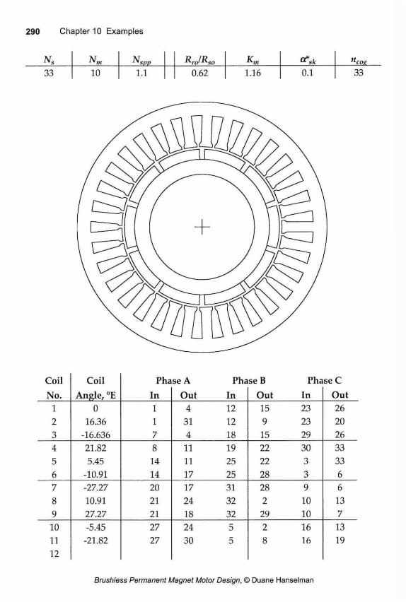
Ns K , N * spp

RJRso K»t ncox

33 10 1.1 0.62 1.16 0.1 33

Coil Coil Phase A Phase B Phase C No. Angle, °E In Out In Out In Out

1 0 1 4 12 15 23 26 2 16.36 1 31 12 9 23 20 3 -16.636 7 4 18 15 29 26 4 21.82 8 11 19 22 30 33 5 5.45 14 11 25 22 3 33 6 -10.91 14 17 25 28 3 6 7 -27.27 20 17 31 28 9 6 8 10.91 21 24 32 2 10 13 9 27.27 21 18 32 29 10 7 10 -5.45 27 24 5 2 16 13 11 -21.82 27 30 5 8 16 19 12

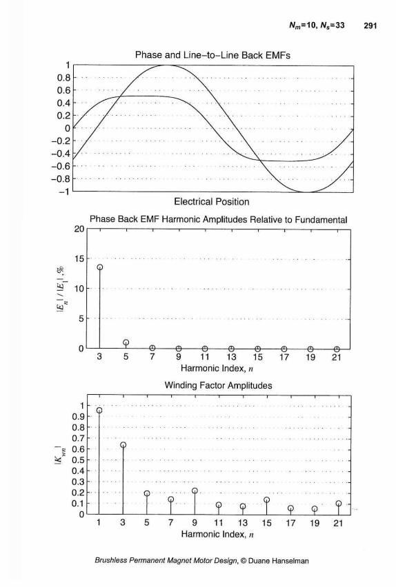
Nm= 10, Ns-33

Electrical Position

Phase Back EMF Harmonic Amplitudes Relative to Fundamental 201—i r-

7 9 11 13 15 Harmonic Index, n

Winding Factor Amplitudes

1 0.9 0.8 0.7 0.6 0.5 0.4 0.3 0.2 0.1

0

Q

Q

Q Q î I ? 9 Î _î 1 7 9 11 13 15 17 19 21

Harmonic Index, n

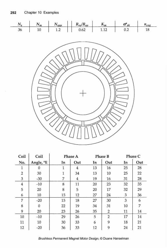
"s Nm N RJRso Km «*sfc "eoe 36 10 1.2 0.62 1.12 0.2 18

Coil Coil Phase A Phase B Phase C No. Angle, °E In Out In Out In Out

1 0 1 4 13 16 25 28 2 30 1 34 13 10 25 22 3 -30 7 4 19 16 31 28 4 -10 8 11 20 23 32 35 5 20 8 5 20 17 32 29 6 10 15 12 27 24 3 36 7 -20 15 18 27 30 3 6 8 0 22 19 34 31 10 7 9 20 23 26 35 2 11 14 10 -10 29 26 5 2 17 14 11 10 30 33 6 9 18 21 12 -20 36 33 12 9 24 21

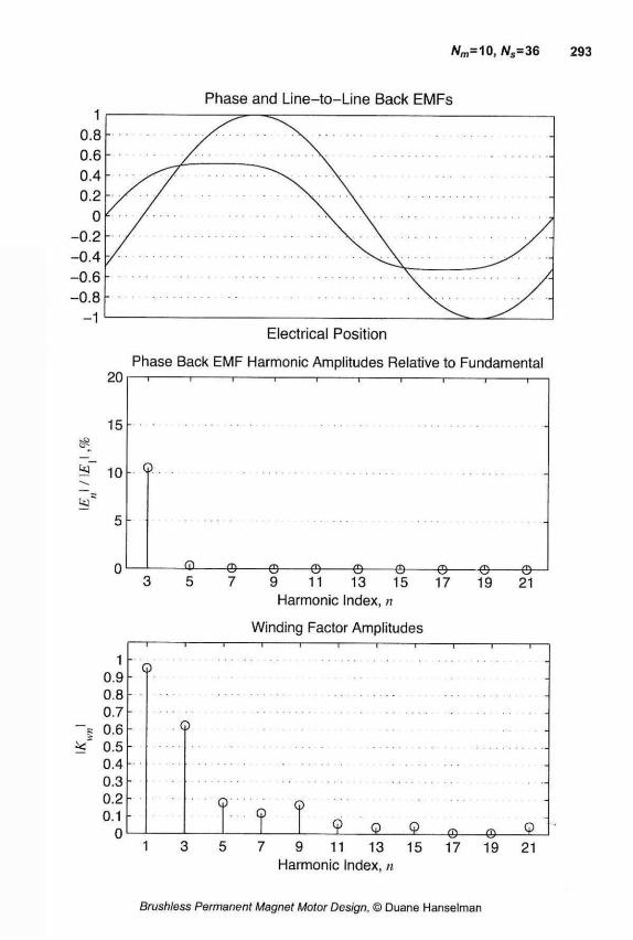
Wm=10, Ns=36

Electrical Position

Phase Back EMF Harmonic Amplitudes Relative to Fundamental

7 9 11 13 15 Harmonic Index, n

Winding Factor Amplitudes

3 5 7 9 11 13 15 Harmonic Index, n

19 21

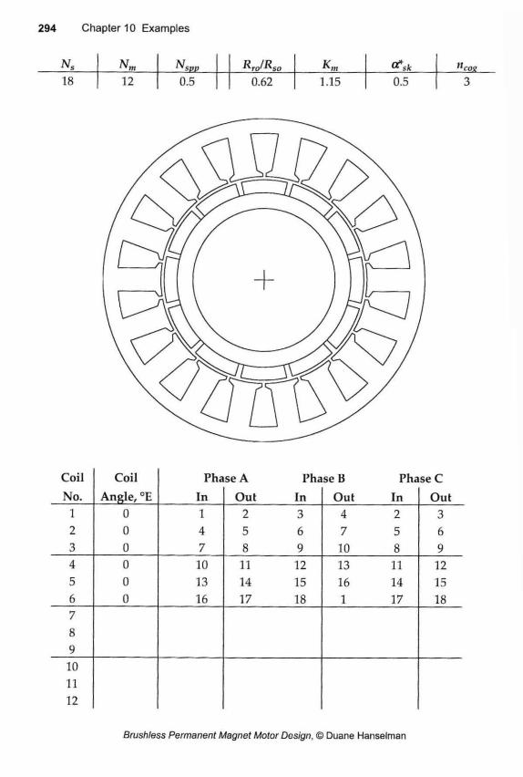
Ns Nm ^svit Rro/R so a*Sk "eoe 18 12 0.5 0.62 1.15 0.5 3

Coil Coil Phase A Phase B Phase C No. Angle, °E In Out In Out In Out

1 0 1 2 3 4 2 3 2 0 4 5 6 7 5 6 3 0 7 8 9 10 8 9 4 0 10 11 12 13 11 12 5 0 13 14 15 16 14 15 6 0 16 17 18 1 17 18 7 8 9 10 11 12

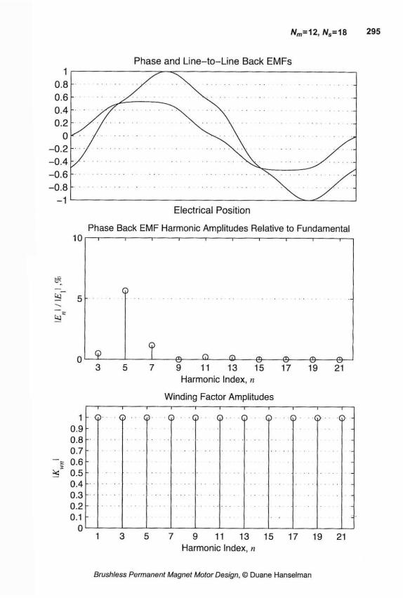
Nm=12, Ns=18

Phase Back EMF Harmonic Amplitudes Relative to Fundamental 101—î 1 1 1 r-

7 9 11 13 15 Harmonic Index, n

Winding Factor Amplitudes î 1 1 1 1 1—

1 3 5 7 9 11 13 15 17 19 21 Harmonic Index, n

Electrical Position

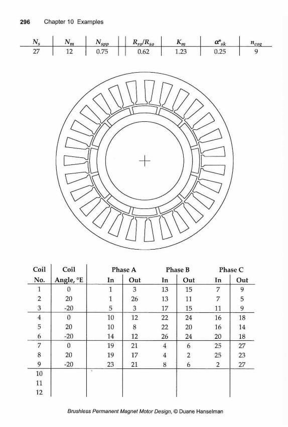
Ns N m NSpp RJRso "eoe 27 12 0.75 0.62 1.23 0.25 9

Coil Coil Phase A Phase B Phase C No. Angle, °E In Out In Out In Out

1 0 1 3 13 15 7 9 2 20 1 26 13 11 7 5 3 -20 5 3 17 15 11 9 4 0 10 12 22 24 16 18 5 20 10 8 22 20 16 14 6 -20 14 12 26 24 20 18 7 0 19 21 4 6 25 27 8 20 19 17 4 2 25 23 9 -20 23 21 8 6 2 27 10 11 12

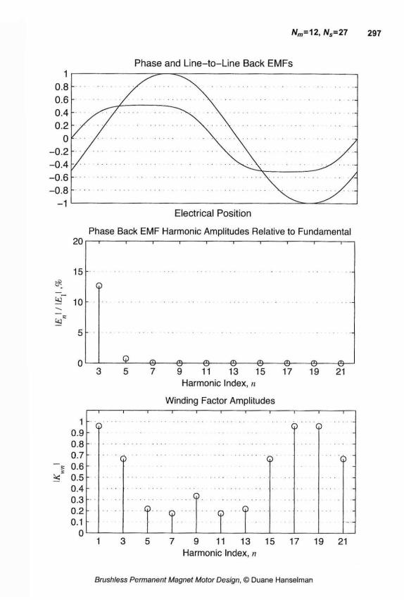
Phase Back EMF Harmonic Amplitudes Relative to Fundamental 201—î 1 1 r

7 9 11 13 15 Harmonic Index, n

Winding Factor Amplitudes

3 5 7 9 11 13 15 17 19 21 Harmonic Index, n

Electrical Position

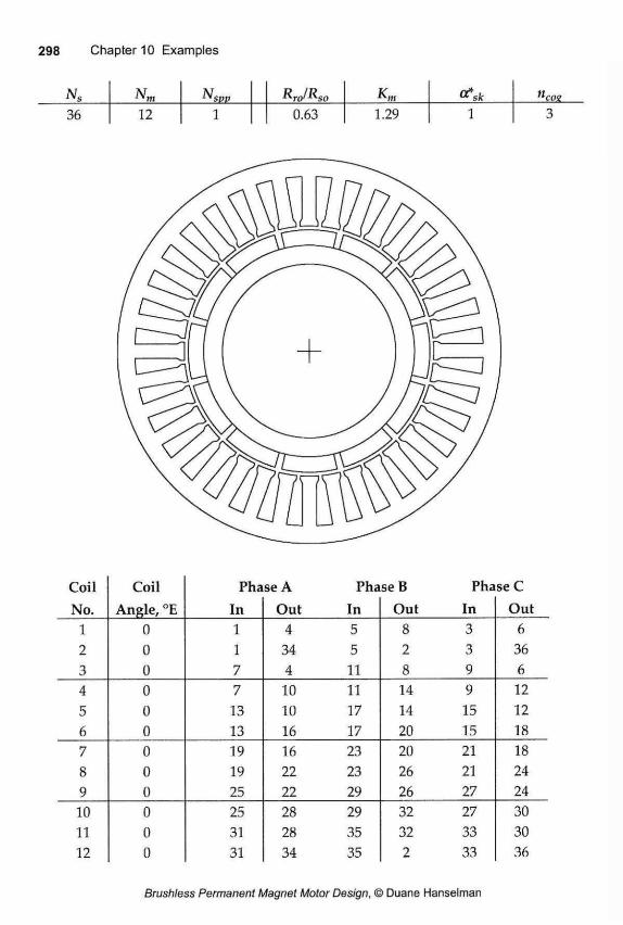
Ns Nm N RJRso a*sfc "eoe 36 12 1 0.63 1.29 1 3

Coil Coil Phase A Phase B Phase C No. Angle, °E In Out In Out In Out

1 0 1 4 5 8 3 6 2 0 1 34 5 2 3 36 3 0 7 4 11 8 9 6 4 0 7 10 11 14 9 12 5 0 13 10 17 14 15 12 6 0 13 16 17 20 15 18 7 0 19 16 23 20 21 18 8 0 19 22 23 26 21 24 9 0 25 22 29 26 27 24 10 0 25 28 29 32 27 30 11 0 31 28 35 32 33 30 12 0 31 34 35 2 33 36

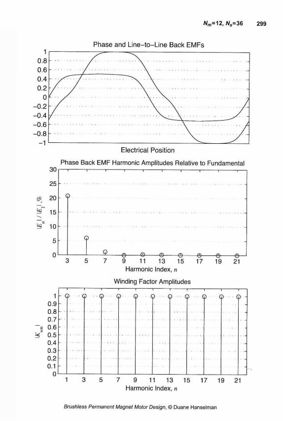
Wm=12, A/s=36 299

Electrical Position

Phase Back EMF Harmonie Amplitudes Relative to Fundamental

9 11 13 15 17 19 21 Harmonie Index, n

Winding Factor Amplitudes

1 0.9 0.8 0.7 0.6 0.5 0.4 0.3 0.2 0.1

0

- Q © © © © © © © © Q

1 3 5 7 9 11 13 15 17 19 21 Harmonie Index, n

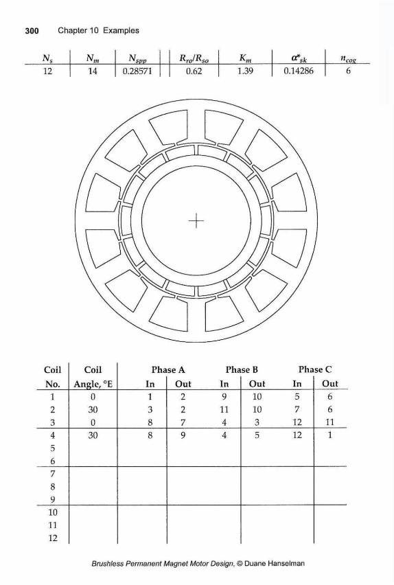
Ns NM N RJRSO KM a*st ^COG 12 14 0.28571 0.62 1.39 0.14286 6

Coil Coil Phase A Phase B Phase C No. Angle, °E In Out In Out In Out

1 0 1 2 9 10 5 6 2 30 3 2 11 10 7 6 3 0 8 7 4 3 12 11 4 30 8 9 4 5 12 1 5 6 7

O 9 10 11 12

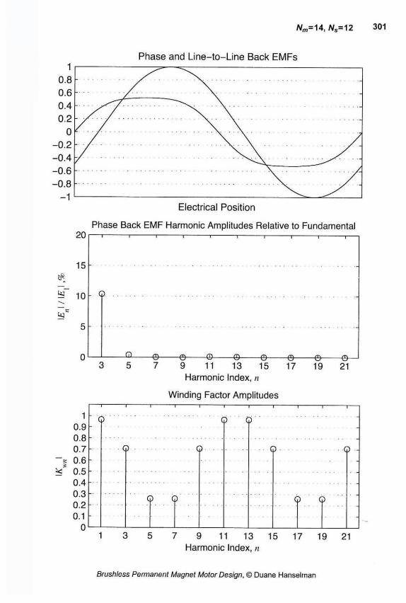
Electrical Position

Phase Back EMF Harmonic Amplitudes Relative to Fundamental 20 I 1 1 1 r i r

1 0.9 0.8 0.7 0.6 0.5 0.4 0.3 0.2 0.1

0

9 11 13 15 Harmonic Index, n

Winding Factor Amplitudes -i 1 1 j—

0 Q

19 21

<P Q Q •

Q Q Q

7 9 11 13 15 17 19 21 Harmonic Index, n

Q

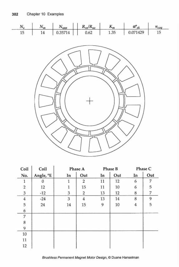
Ns Nm N RJRso 0?sk "eoe 15 14 0.35714 0.62 1.35 0.071429 15

Coil Coil Phase A Phase B Phase C No. Angle, °E In Out In Out In Out

1 0 1 2 11 12 6 7 2 12 1 15 11 10 6 5 3 -12 3 2 13 12 8 7 4 -24 3 4 13 14 8 9 5 24 14 15 9 10 4 5 6 7 o o 9 10 11 12

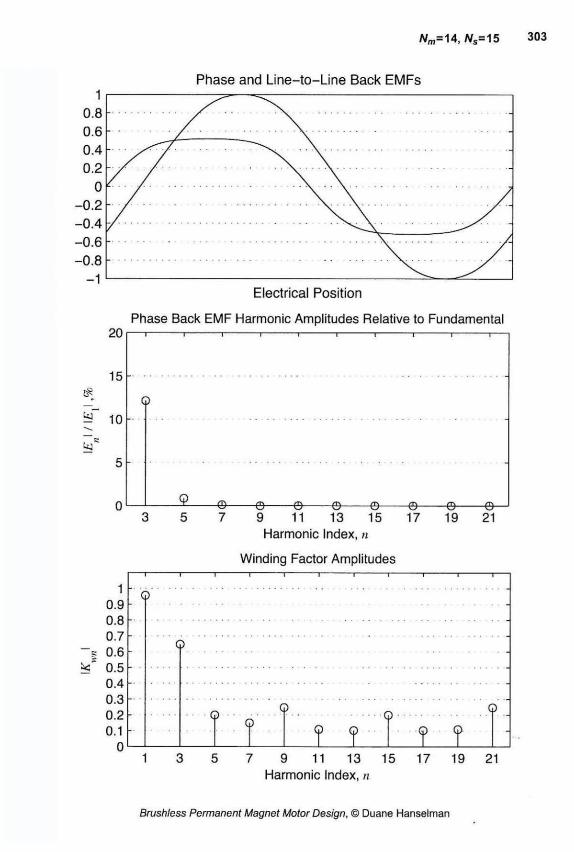
Electrical Position

Phase Back EMF Harmonic Amplitudes Relative to Fundamental 201—i 1 r-

7 9 11 13 15 Harmonic Index, n

Winding Factor Amplitudes

19 21

1 0.9 0.8 0.7 0.6 0.5 0.4 0.3 0.2 0.1

0

I I I I Q

Q Q Q T ?

Q Q

7 9 11 13 15 17 19 21 Harmonic Index, n

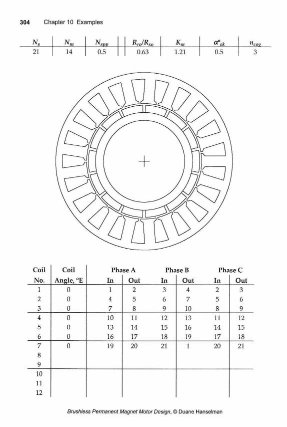
Ns N m N SVP

RJRsc "eoe 21 14 0.5 0.63 1.21 0.5 3

Coil Coil Phase A Phase B Phase C No. Angle, °E In Out In Out In Out

1 0 1 2 3 4 2 3 2 0 4 5 6 7 5 6 3 0 7 8 9 10 8 9 4 0 10 11 12 13 11 12 5 0 13 14 15 16 14 15 6 0 16 17 18 19 17 18 7 Q

0 19 20 21 1 20 21

9 10 11 12

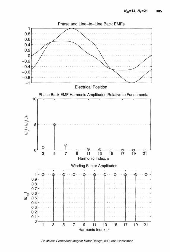
3 5 7 9 11 13 15 17 19 21 Harmonic Index, n

Phase Back EMF Harmonic Amplitudes Relative to Fundamental 10 — I 1 1 1 1 1 1 1 1 1—

Winding Factor Amplitudes

Electrical Position

m m yj m m m m 9 11 13 15 17 19 21 Harmonie Index, n

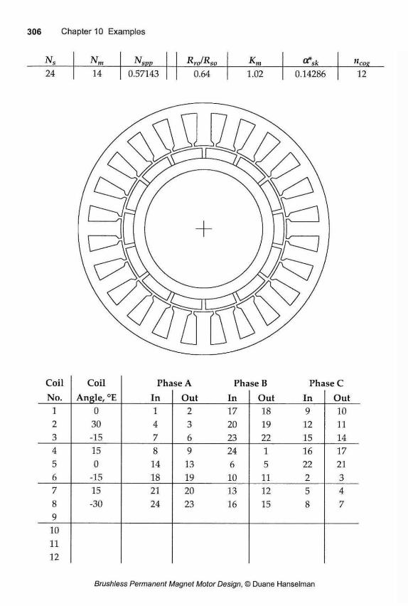
Ns N m NSpt> Rro/Rso Km 24 14 0.57143 0.64 1.02 0.14286 12

Coil Coil Phase A Phase B Phase C No. Angle, °E In Out In Out In Out

1 0 1 2 17 18 9 10 2 30 4 3 20 19 12 11 3 -15 7 6 23 22 15 14 4 15 8 9 24 1 16 17 5 0 14 13 6 5 22 21 6 -15 18 19 10 11 2 3 7 15 21 20 13 12 5 4 8 -30 24 23 16 15 8 7 9 10 11 12

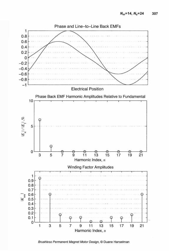
Electrical Position

Phase Back EMF Harmonic Amplitudes Relative to Fundamental

7 9 11 13 15 Harmonic Index, n

Winding Factor Amplitudes

7 9 11 13 15 Harmonic Index, n

19 21

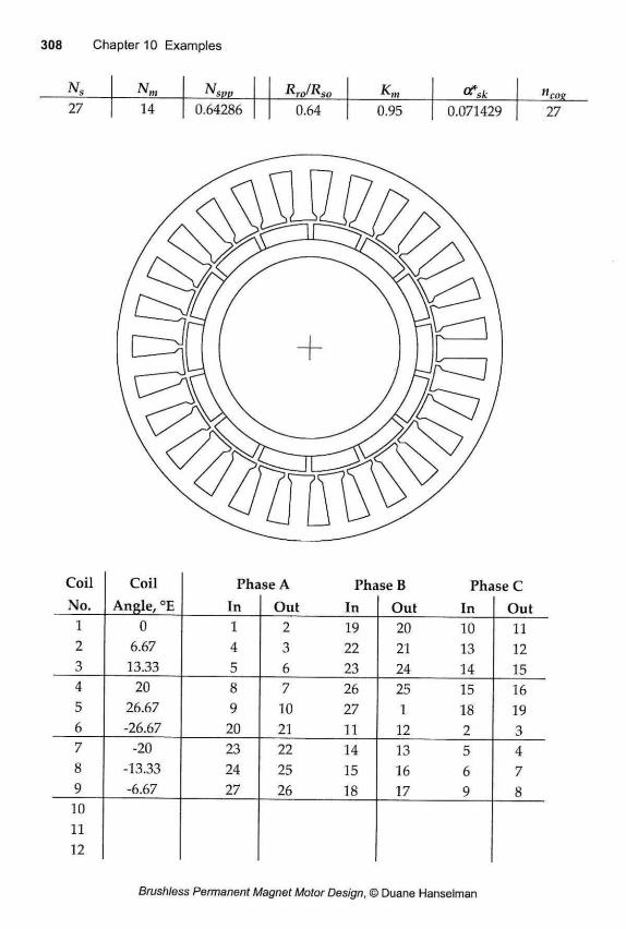
Nm N Rr0/Rs0 Km 27 14 0.64286 0.64 0.95 0.071429 27

Coil Coil Phase A Phase B Phase C No. Angle, °E In Out In Out In Out

1 0 1 2 19 20 10 11 2 6.67 4 3 22 21 13 12 3 13.33 5 6 23 24 14 15 4 20 8 7 26 25 15 16 5 26.67 9 10 27 1 18 19 6 -26.67 20 21 11 12 2 3 7 -20 23 22 14 13 5 4 8 -13.33 24 25 15 16 6 7 9 -6.67 27 26 18 17 9 8 10 11 12

Electrical Position

Phase Back EMF Harmonic Amplitudes Relative to Fundamental

7 9 11 13 15 Harmonic Index, n

Winding Factor Amplitudes

3 5 7 9 11 13 15 17 19 21 Harmonic Index, n

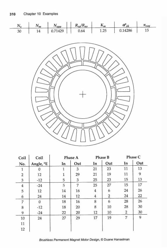
Ns Nm N RJRso Km 0?sk " cog

30 14 0.71429 0.64 1.25 0.14286 15

Coil Coil Phase A Phase B Phase C

No. Angle, °E In Out In Out In Out 1 0 1 3 21 23 11 13 2 12 1 29 21 19 11 9 3 -12 5 3 25 23 15 13 4 -24 5 7 25 27 15 17 5 12 14 16 4 6 24 26 6 24 14 12 4 2 24 22 7 0 18 16 8 6 28 26 8 -12 18 20 8 10 28 30 9 -24 22 20 12 10 2 30 10 24 27 29 17 19 7 9 11 12

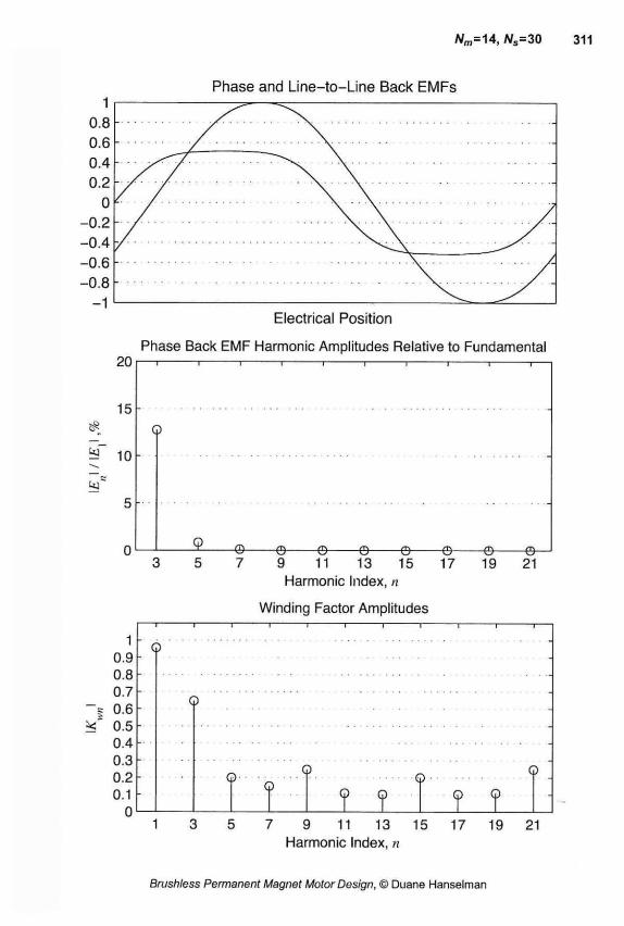
Electrical Position

Phase Back EMF Harmonic Amplitudes Relative to Fundamental 20 I i 1 r

7 9 11 13 15 Harmonic Index, n

Winding Factor Amplitudes

3 5 7 9 11 13 15 17 19 21 Harmonic Index, n

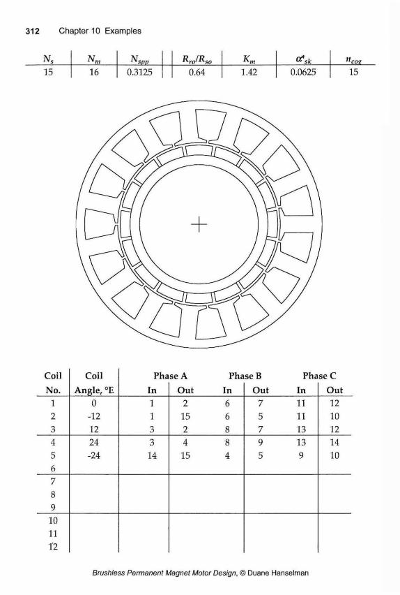
Ns Nm N Km ncot

15 16 0.3125 0.64 1.42 0.0625 15

Coil Coil Phase A Phase B Phase C No. Angle, °E In Out In Out In Out

1 0 1 2 6 7 11 12 2 -12 1 15 6 5 11 10 3 12 3 2 8 7 13 12 4 24 3 4 8 9 13 14 5 -24 14 15 4 5 9 10 6 7

O 9 10 11 Ï2

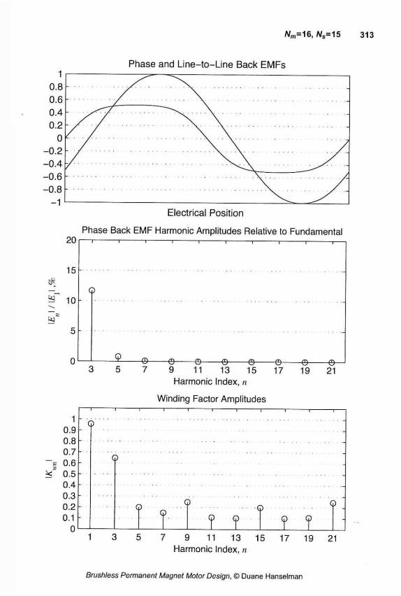
Wm=16, Ns=15 313

Phase Back EMF Harmonic Amplitudes Relative to Fundamental

7 9 11 13 15 Harmonic Index, n

Winding Factor Amplitudes

7 9 11 13 15 17 19 21 Harmonic Index, n

Electrical Position

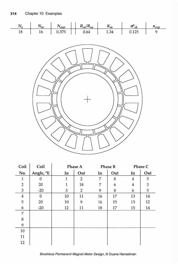
N,„ NSpp RnJRso Kn tf'sk ncog

18 16 0.375 0.64 1.34 0.125 9

Coil Coil Phase A Phase B Phase C No. Angle, °E In Out In Out In Out

1 0 1 2 7 8 4 5 2 20 1 18 7 6 4 3 3 -20 3 2 9 8 6 5 4 0 10 11 16 17 13 14 5 20 10 9 16 15 13 12 6 -20 12 11 18 17 15 14 7 8 9 10 11 12

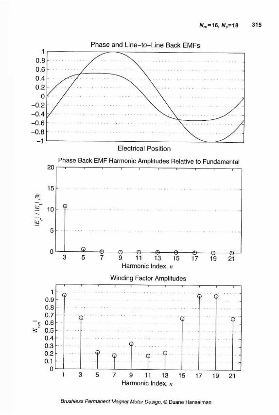
A/m=16, Ns= 18 315

Phase Back EMF Harmonic Amplitudes Relative to Fundamental

9 11 13 15 Harmonic Index, n

1 0.9 0.8 0.7 - g 0.6

* 0.5 0.4 0.3 0.2 0.1

0

Electrical Position

1 3 5 7 9 11 13 15 17 19 21 Harmonic Index, n

Winding Factor Amplitudes I 1 I 1 1 1 1 1—

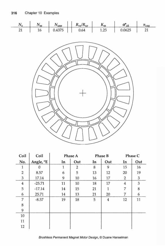
Nm Nspp RJRso 1 1 cog

21 16 0.4375 0.64 1.25 0.0625 21

Coil Coil Phase A Phase B Phase C No. Angle, °E In Out In Out In Out

1 0 1 2 8 9 15 16 2 8.57 6 5 13 12 20 19 3 17.14 9 10 16 17 2 3 4 -25.71 11 10 18 17 4 3 5 -17.14 14 15 21 1 7 8 6 25.71 14 13 21 20 7 6 7 -8.57 19 18 5 4 12 11

O 9 10 11 12

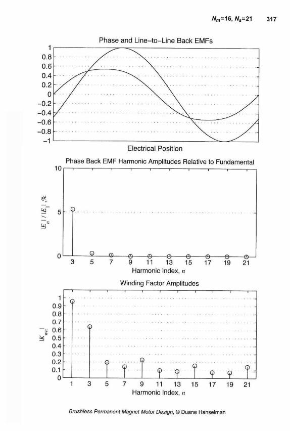
-e © © © © ©-9 11 13 15 17 19 21 Harmonic Index, n

Winding Factor Amplitudes

3 5 7 9 11 13 15 17 19 21 Harmonic Index, n

Phase Back EMF Harmonic Amplitudes Relative to Fundamental 10 1 1 1 1 r- 1 1 1 1 1

Electrical Position

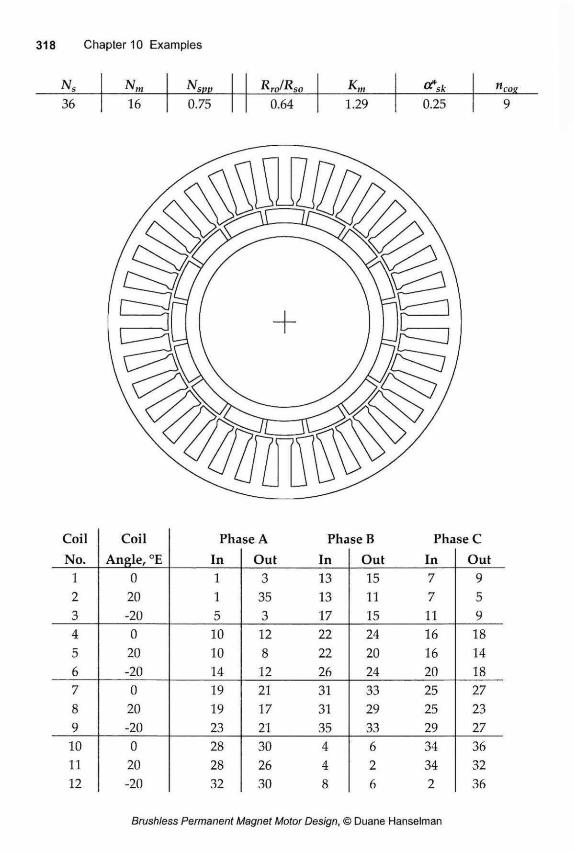
Ns Nm N Rro/Rso "cos 36 16 0.75 0.64 1.29 0.25 9

Coil Coil Phase A Phase B Phase C No. Angle, °E In Out In Out In Out

1 0 1 3 13 15 7 9 2 20 1 35 13 11 7 5 3 -20 5 3 17 15 11 9 4 0 10 12 22 24 16 18 5 20 10 8 22 20 16 14 6 -20 14 12 26 24 20 18 7 0 19 21 31 33 25 27 8 20 19 17 31 29 25 23 9 -20 23 21 35 33 29 27 10 0 28 30 4 6 34 36 11 20 28 26 4 2 34 32 12 -20 32 30 8 6 2 36

Wm=16, A/s=36

Electrical Position

Phase Back EMF Harmonic Amplitudes Relative to Fundamental 20 I — r

7 9 11 13 15 Harmonic Index, n

Winding Factor Amplitudes

3 5 7 9 11 13 15 17 19 21 Harmonic Index, n

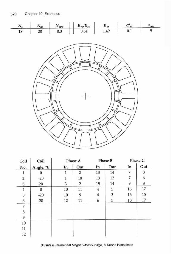
Ns N m N s p ( ) RJRso C?sk " cog

18 20 0.3 0.64 1.49 0.1 9

Coil Coil Phase A Phase B Phase C

No. Angle, °E In Out In Out In Out 1 0 1 2 13 14 7 8 2 -20 1 18 13 12 7 6 3 20 3 2 15 14 9 8 4 0 10 11 4 5 16 17 5 -20 10 9 4 3 16 15 6 20 12 11 6 5 18 17 7

O 9 10 11 12

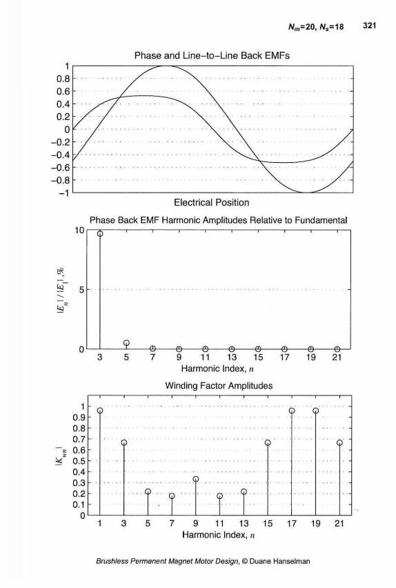
Electrical Position

Phase Back EMF Harmonic Amplitudes Relative to Fundamental 1 0 r w

7 9 11 13 15 Harmonic Index, n

Winding Factor Amplitudes

3 5 7 9 11 13 15 17 19 21 Harmonic Index, n

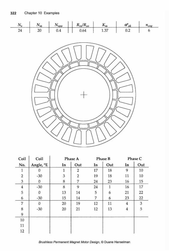
Ns N m TV RJRso Km "coj? 24 20 0.4 0.64 1.3 7 0.2 6

Coil Coil Phase A Phase B Phase C No. Angle, °E In Out In Out In Out

1 0 1 2 17 18 9 10 2 -30 3 2 19 18 11 10 3 0 8 7 24 23 16 15 4 -30 8 9 24 1 16 17 5 0 13 14 5 6 21 22 6 -30 15 14 7 6 23 22 7 0 20 19 12 11 4 3 8 -30 20 21 12 13 4 5 9 10 11 12

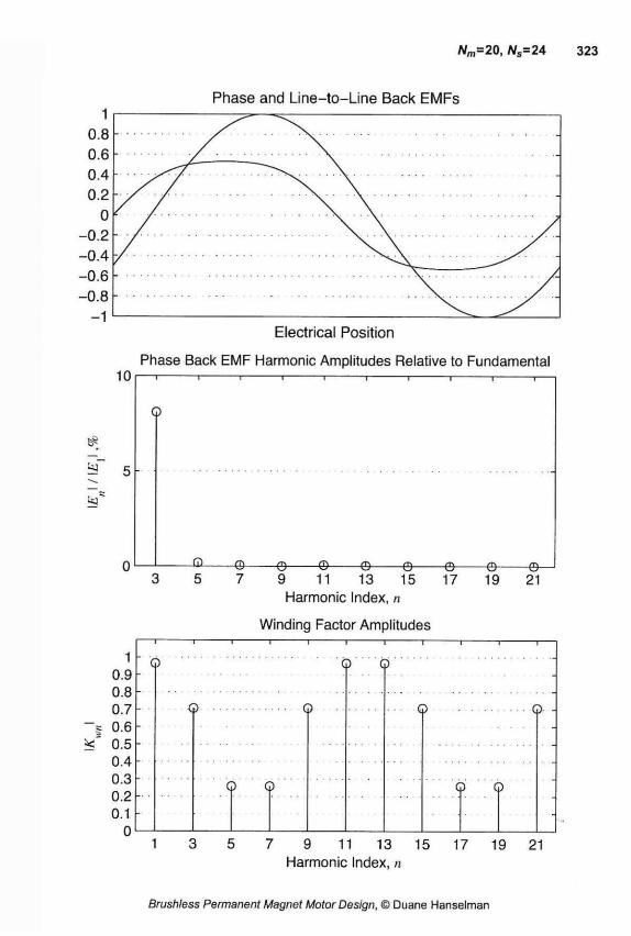
Phase Back EMF Harmonic Amplitudes Relative to Fundamental

9 11 13 15 17 19 21 Harmonic Index, n

Winding Factor Amplitudes

3 5 7 9 11 13 15 17 19 21 Harmonic Index, n

1 0.8

0.6 0.4 0.2

0 - 0 . 2

- 0 . 4 - 0 . 6

- 0 . 8

- 1

Electrical Position

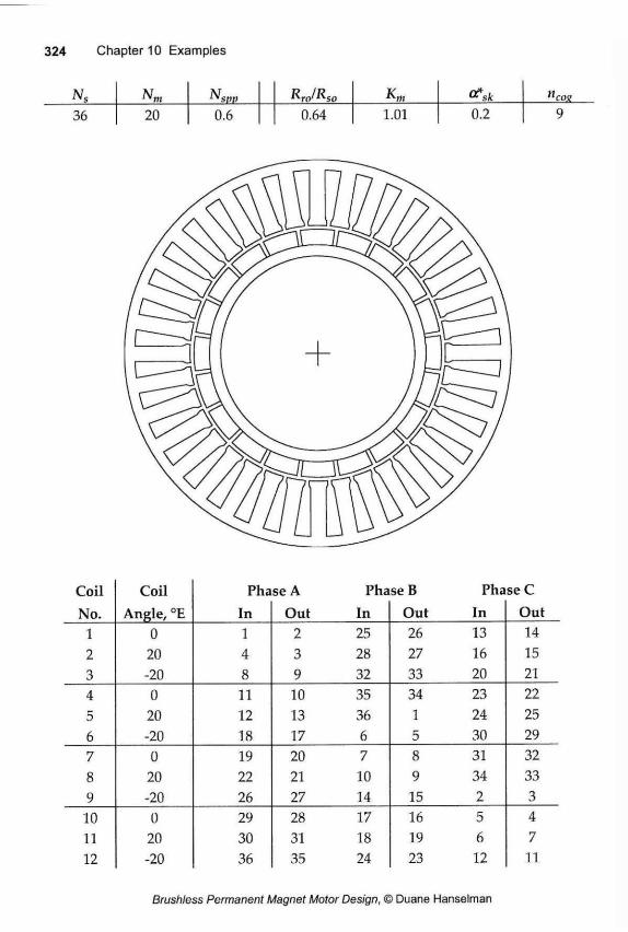
Ns N m N s v v R J R S 0 Km ncos

36 20 0.6 0.64 1.01 0.2 9

Coil Coil Phase A Phase B Phase C No. Angle, °E In Out In Out In Out

1 0 1 2 25 26 13 14 2 20 4 3 28 27 16 15 3 -20 8 9 32 33 20 21 4 0 11 10 35 34 23 22 5 20 12 13 36 1 24 25 6 -20 18 17 6 5 30 29 7 0 19 20 7 8 31 32 8 20 22 21 10 9 34 33 9 -20 26 27 14 15 2 3 10 0 29 28 17 16 5 4 11 20 30 31 18 19 6 7 12 -20 36 35 24 23 12 11

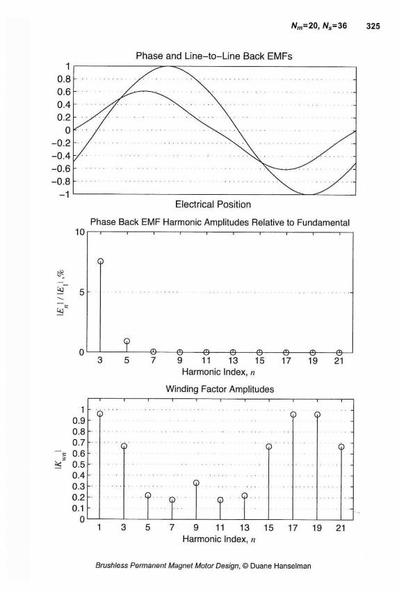
Electrical Position

Phase Back EMF Harmonic Amplitudes Relative to Fundamental

7 9 11 13 15 Harmonic Index, n

Winding Factor Amplitudes

19 21

1 0.9 0.8 0.7 0.6 0.5 0.4 0.3 0.2 0.1

0

1 r -I 1 1 1 r Q Q

Q 9

Q Q Q' Q

Q

5 7 9 11 13 15 17 19 21 Harmonic Index, n

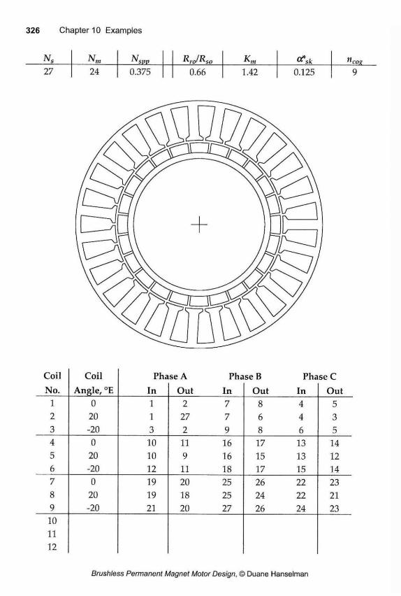
iVs Nm NSvv RJRso <?sk "cos 27 24 0.375 0.66 1.42 0.125 9

Coil Coil Phase A Phase B Phase C No. Angle, °E In Out In Out In Out

1 0 1 2 7 8 4 5 2 20 1 27 7 6 4 3 3 -20 3 2 9 8 6 5 4 0 10 11 16 17 13 14 5 20 10 9 16 15 13 12 6 -20 12 11 18 17 15 14 7 0 19 20 25 26 22 23 8 20 19 18 25 24 22 21 9 -20 21 20 27 26 24 23 10 11 12

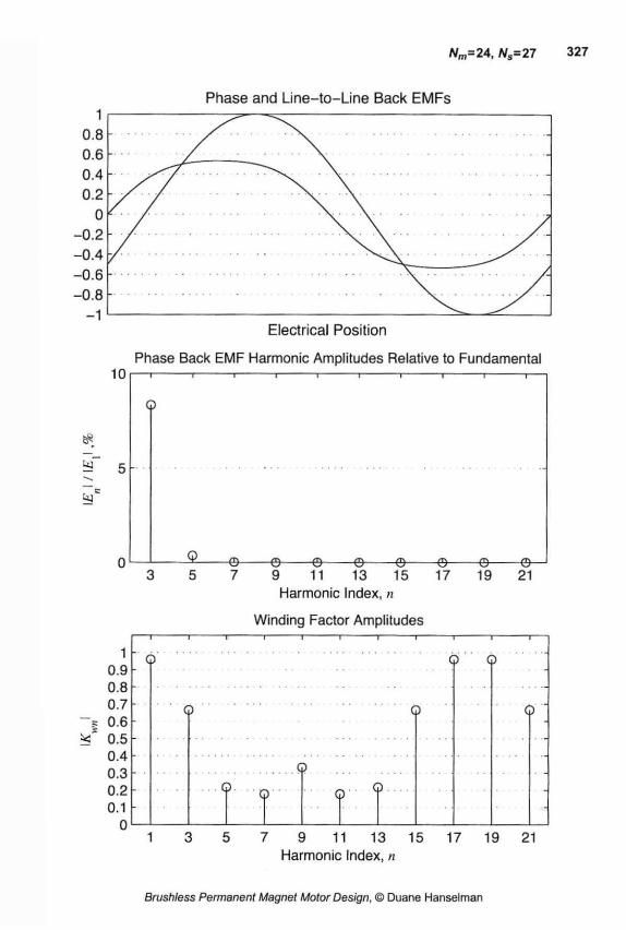
Nm=24, Ns= 27 327

Electrical Position

Phase Back EMF Harmonic Amplitudes Relative to Fundamental 10 I 1 r -

7 9 11 13 15 Harmonic Index, n

Winding Factor Amplitudes

1 0.9 0.8 0.7 0.6 0.5 0.4 0.3 0.2 0.1

0

Q

© Q. Q

Q

3 5 7 9 11 13 15 17 19 21 Harmonic Index, n

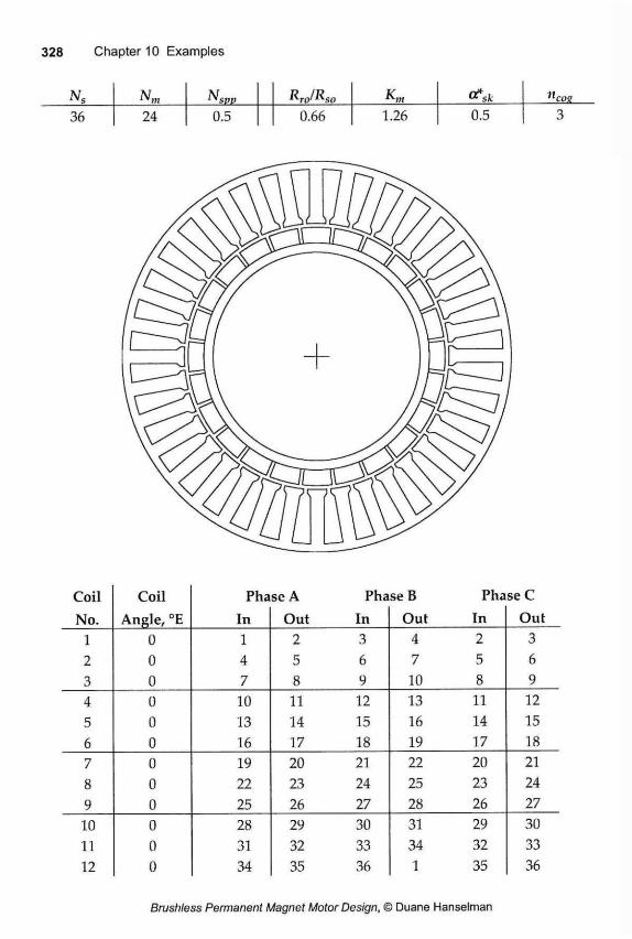
Ns Nm N RJRso ncos 36 24 0.5 0.66 1.26 0.5 3

Coil Coil Phase A Phase B Phase C No. Angle, °E In Out In Out In Out

1 0 1 2 3 4 2 3 2 0 4 5 6 7 5 6 3 0 7 8 9 10 8 9 4 0 10 11 12 13 11 12 5 0 13 14 15 16 14 15 6 0 16 17 18 19 17 18 7 0 19 20 21 22 20 21 8 0 22 23 24 25 23 24 9 0 25 26 27 28 26 27 10 0 28 29 30 31 29 30 11 0 31 32 33 34 32 33 12 0 34 35 36 1 35 36

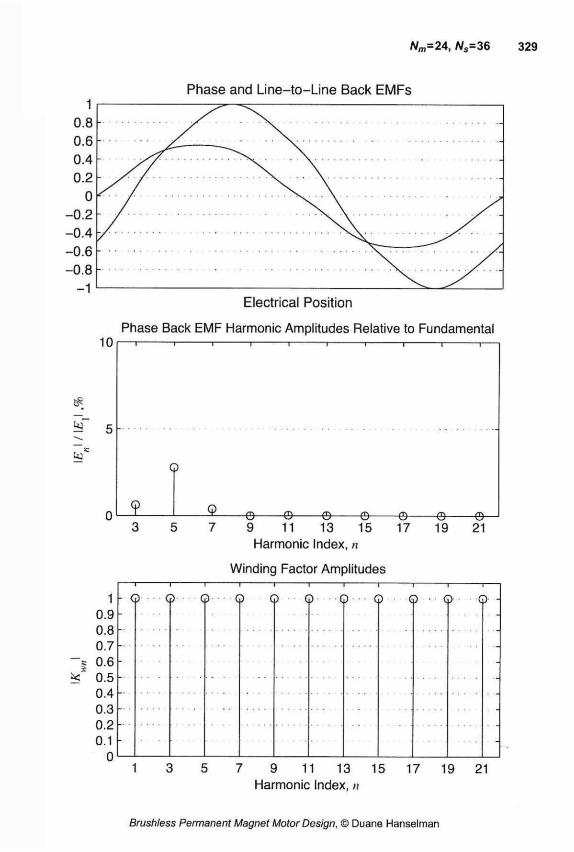
1 0.8 0 .6 0.4 0.2

0 - 0 . 2

- 0 . 4 - 0 . 6

- 0 . 8

- 1

Electrical Position

Phase Back EMF Harmonic Amplitudes Relative to Fundamental 10

Ü f 5

0

1 0.9 0.8 0.7

- § 0 .6 * 0.5

0.4 0.3 0.2 0.1

0

9 11 13 15 Harmonic Index, n

Winding Factor Amplitudes

- © Q © © Q © © © © © -

1 3 5 7 9 11 13 15 17 19 21 Harmonic Index, n

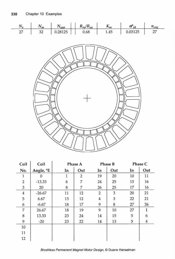
N RJRso Km a*sfc "cos 27 32 0.28125 0.68 1.45 0.03125 27

Coil Coil Phase A Phase B Phase C No. Angle, °E In Out In Out In Out

1 0 1 2 19 20 10 11 2 -13.33 6 7 24 25 15 16 3 20 8 7 26 25 17 16 4 -26.67 11 12 2 3 20 21 5 6.67 13 12 4 3 22 21 6 -6.67 18 17 9 8 27 26 7 26.67 18 19 9 10 27 1 8 13.33 23 24 14 15 5 6 9 -20 23 22 14 13 5 4 10 11 12

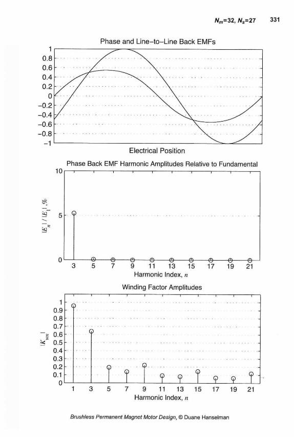
1 0.8 0 .6 0.4 0.2

0 - 0 . 2

- 0 . 4 - 0 . 6

- 0 . 8

- 1

Phase Back EMF Harmonic Amplitudes Relative to Fundamental 10

tS

ä" 5

is*

0

1 0.9 0.8 0.7

- g 0.6 ^ 0.5

0.4 0.3 0.2 0.1

0

7 9 11 13 15 Harmonic Index, n

Winding Factor Amplitudes

7 9 11 13 15 17 19 21 Harmonic Index, n

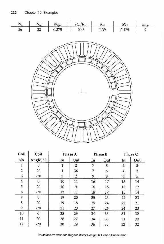
Ns Nm N RJRso Km 0?sk "cos 36 32 0.375 0.68 1.39 0.125 9

Coil Coil Phase A Phase B Phase C No. Angle, °E In Out In Out In Out

1 0 1 2 7 8 4 5 2 20 1 36 7 6 4 3 3 -20 3 2 9 8 6 5 4 0 10 11 16 17 13 14 5 20 10 9 16 15 13 12 6 -20 12 11 18 17 15 14 7 0 19 20 25 26 22 23 8 20 19 18 25 24 22 21 9 -20 21 20 27 26 24 23 10 0 28 29 34 35 31 32 11 20 28 27 34 33 31 30 12 -20 30 29 36 35 33 32

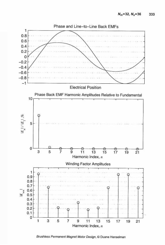
Nm=32, Ns= 36

Electrical Position

Phase Back EMF Harmonic Amplitudes Relative to Fundamental

7 9 11 13 15 Harmonic Index, n

Winding Factor Amplitudes

1 0.9 0.8 0.7 0.6 0.5 0.4 0.3 0.2 0.1

0

O Q Q

Q Q

P . . Q Q <p

3 5 7 9 11 13 15 17 19 21 Harmonic Index, n

Appendix A Fourier Series

Fourier series can be applied to many aspects of motor analysis since rotary actuators are inherently periodic. This appendix contains basic information that supports the use of Fourier series in this text. Because periodicity in this text is with respect to angle 0, the treatment that follows uses 6 instead of co0t as the fundamental argu-ment.

A.1 Definition

There are three common forms for the Fourier series. They are (a) the trigonometric form

f (6) = a0 + cos(n6) + bn sin(n6) (A.1)

the alternate trigonometric form

(A.2) «=i

and the exponential form

m^iLfn^ (A.3)

where j = V^l , n is the harmonic number or index, and a,u bn, cn, and/„ are Fourier series coefficients.

Of these forms, the trigonometric is convenient because sine and cosine evoke clear visual images. On the other hand, the exponential is easiest to manipulate mathe-matically because only one set of coefficients exists. For this reason, this text concen-trates on the exponential form.

A.2 Coefficients

All of the above Fourier series descriptions are equivalent. Given one form, the other forms are easily found by converting Fourier series coefficients from one form to another. The following equations summarize the relationships among the coefficients

ao=co = fo

fl„=2Re(/„)

b„ - ~2Im(/„ )

ipn = tan -1 — (A.4) "n

Because the Fourier series forms are related simply, it is beneficial to use the expo-nential form mathematically, and then convert results to the trigonometric form for display when desired.

The coefficients for the exponential form are given by

where the integration is over any period of length 2K. These coefficients form a com-plex conjugate set whenf(0) is a real-valued function, that is

fn=f-n (A.6)

where * denotes complex conjugation. Therefore, it is only necessary to compute the positive coefficients and use (A.6) to find the negative coefficients.

A.3 Symmetry Properties

Sometimes f(6) has identifiable symmetry properties. When this occurs, the computa-tion of Fourier series coefficients is simplified. More importantly coefficients become real or imaginary, or some coefficients become zero.

When f(0)= f(-0), the function is said to be even. In this case, the Fourier coefficients have zero imaginary part, i.e., fn~Re(f„). In addition, (A.5) can be rewritten as

f„=^[f(9)cos(nd)de (A.7)

When/(#)=-/(-$), the function is said to be odd. In this case, the Fourier coefficients have zero real part, i.e., fn=\vt\{fn). In addition, (A.5) can be rewritten as

fn=-j^[f(e)sm(nd)d6 (A.8)

In addition to these basic symmetries, when f(6)=-f{-&Jrïï), the function is said to have odd halfwave symmetry. In this case, the function has the same shape every half period, except for a sign change. This symmetry appears often in brushless perma-nent magnet motor waveforms and therefore is important to recognize. In this case, the Fourier coefficients are zero for all even indices n. That is, the waveform contains odd harmonics only. In this case, (A.5) can be rewritten as

fn = - T /(0)e~'"edd n odd * J ü (A.9)

0 n even

Odd halfwave symmetry is independent of even and odd symmetry. Therefore a waveform can have both halfwave symmetry and even symmetry, in which case all coefficients are real and only odd harmonics exist. A similar statement can be made for waveforms that exhibit both odd and halfwave symmetries.

A.4 Mathematical Operations

Given a waveform f(6) described by an exponential Fourier series (A.3), it is possible to relate mathematical operations on/(0) to operations on the Fourier series coeffi-cients. In doing so, the resulting waveform has a Fourier series description as well. In the expression that follow, f(6), g(6) and h(6) have the Fourier series expansions

g(0)= X (A.10)

MÖ)=X h*eik6

Addition Given the sum of two functions, h(6)=f(0)+g(9), the Fourier series coefficients of the sum are

That is, the Fourier series coefficients of the sum of two functions is simply the sum of the corresponding coefficients.

Scalar Multiplication Given the product g(d)=Kf($), where K is a constant, the Fourier series coefficients of the product are

So scalar multiplication simply scales all Fourier series coefficients by the scalar.

Function Product Given the product of two functions, h(0)=f(6)g(6), the Fourier series coefficients of the product are

These expressions show that the Fourier series coefficients of a product are given by the discrete convolution of the coefficients constituting the product.

Phase Shift If two functions are related by a phase shift as g(0)=/(0-0), then the Fourier series coefficients of g(6) are given by

K=fn+g,i (A/11)

Sn=Kfn (A.12)

(A.13)

(A.14)

This expression and (A.13) demonstrate the utility of the exponential form of the Fourier series. No such simple relationships for function product and phase shift appear for the trigonometric forms of the Fourier series.

Differentiation The derivative of a function having a Fourier series description, produces another Fourier series. In the case of the exponential form, this relationship is simple. Given g(Q)=df(6)/d6, the Fourier series coefficients of the derivative are

gn=jnfn (A.15)

Thus, differentiation becomes multiplication by jn.

Mean Square Value and RMS Power is associated with the RMS value of a function and mean square value is sim-ply the square of the RMS value. That is, given a function/(#), its mean square value is defined as

( f ^ h ^ U ^ 2 " 0 <A-16> Substitution of the Fourier series expression for/(0) into (A.16), gives the result

( / ( * ) > ¿ / „ / - „ = i l / „ | 2 (A.17)

The RMS value of a function is the square root of (A.17).

A.5 Computing Coefficients

Often the most difficult aspect of the i\se of Fourier series is the computation of Fou-rier series coefficients. When the function /(#) is simply defined, the Fourier series coefficients can often be computed using the defining integral (A.5). In many cases, the tedium involved in the use of (A.5) can be minimized by using the symbolic alge-bra capabilities available in a number of software packages.

When it becomes too difficult or impossible to use (A.5), the Fourier series coeffi-cients can be computed numerically using the Fast Fourier Transform (FFT). The FFT

algorithm forms the cornerstone of digital signal processing. As a result, most numerically-oriented software packages include functions for its computation.

The following procedure describes use of the function fft(-), which computes the FFT of its argument, to find the exponential Fourier series coefficients for any peri-odic function f(9). The procedure requires that f(6) be evaluated at specified points over one period. If f(6) is a tabulated function, i.e., exists as a table of data points, an interpolation routine must be used to generate the required points.

Procedure a) Choose the number of positive harmonics N such that the amplitude of all

harmonics greater than N are negligible. Often FFT routines require that N

be a power of two, that is, N= 2m, where m is an integer. If N is not chosen sufficiently large, aliasing occurs, which introduces error in the desired coef-ficients. If N is chosen larger than necessary, undesired higher harmonic coefficients can be thrown away. The author has found that N= 64 is suffi-cient for motor design purposes.

b) Evaluate the function f(6) at M=2N+1 equally spaced points between 0 and 2K inclusive, where 2K is the assumed period. That is, evaluate f(9) at the points

Gk=-^-2n k = 0 ,1 ,2 , . . . ,M-1 k M - l

to produce the function valuesfk=f(0k), for /c=0,l,...,M-l.

c) Eliminate the last data point (^m-i/m-i) from this data set, leaving 2N data points. Compute the FFT of the resulting data set, Fk-(it(fk). This produces 2N frequency domain data points denoted Fk, for k=l,2,...,2N.

d) Divide the frequency domain data points by 2N, i.e., Fk=Fk/(2N), for k= 1,2,...,2 N.

e) The DC or »=0 Fourier series coefficient is F^ Using the notation from (A.5), which is not to be confused with the notation in b) and c) above,/q=F1. This value must be real but sometimes has a residual imaginary part. If it does, simply extract the real portion,/o=real(/o).

f) The positive harmonics are the next N points, i.e.,fn=Fn+i, for n=1,2,.. .,N.

g) The negative harmonics are the complex conjugate of the corresponding positive harmonics according to (A.6).

The above procedure is very fast and works well, especially when the number of points chosen is larger than necessary, and the excess harmonics are excluded at the end. Because the FFT is a numerical algorithm, it is common for symmetry properties to be violated. For example, if f(6) is even, its Fourier series coefficients must be real. Use of the FFT may produce results with residual imaginary parts, which violates this symmetry property. When the symmetry properties of f(G) are known, the FFT results can be modified to match the symmetry properties.

A.6 Summary

The exponential form of the Fourier series is conducive to mathematical manipula-tion. The properties and mathematical operations presented here are useful for the analysis and design of brushless permanent magnet motors.

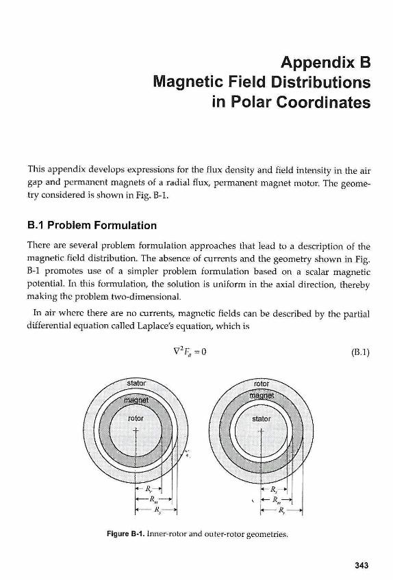
Appendix B Magnetic Field Distributions

in Polar Coordinates

This appendix develops expressions for the flux density and field intensity in the air gap and permanent magnets of a radial flux, permanent magnet motor. The geome-try considered is shown in Fig. B-l.

B.1 Problem Formulation

There are several problem formulation approaches that lead to a description of the magnetic field distribution. The absence of currents and the geometry shown in Fig. B-l promotes use of a simpler problem formulation based on a scalar magnetic potential. In this formulation, the solution is uniform in the axial direction, thereby making the problem two-dimensional.

In air where there are no currents, magnetic fields can be described by the partial differential equation called Laplace's equation, which is

V 2 F a = 0 (B.l)

Figure B-1. Inner-rotor and outer-rotor geometries.

where F„ is the scalar magnetic potential in the air space. In regions containing per-manent magnets, magnetic fields can be described by the quasi-Poisson partial differ-ential equation

n 2 r V - M V Fm= (B.2)

Mr

where Fm is the scalar magnetic potential in the magnet, jjr is the magnet relative recoil permeability, and M is the magnet magnetization. The magnetization of the magnet is the magnetic field source in this problem. It is what causes flux to flow in a manner that obeys (B.l) and (B.2).

If a solution to the above scalar potential equations can be found, the corresponding vector field intensity is computed using

H = -VF (B.3)

where F is either Fa or Fm. Given the field intensity, the vector flux densities in the two regions are given by

Bm=W0Hm+fioM ( B ' 4 )

where n0 is the permeability of free space and the subscripts a and m denote the air and magnet regions respectively.

Specific solutions to (B.l) and (B.2) are found by applying the customary boundary conditions which specify that the tangential component of field intensity and the nor-mal component of the flux density are continuous across material boundaries. Because the ferromagnetic material is assumed to be infinitely permeable, these con-ditions imply that the tangential component of the field intensity is zero at ferromag-netic material boundaries.

Because the air and magnet regions are linear, superposition applies. As a result, if the magnetization M is written as a Fourier series, each term in its Fourier series creates like harmonic terms in the field intensity and flux density. Because of this property, the partial differential equations need only be solved using a general term in the magnetization Fourier series. This general solution then describes a general term in the field intensity and flux density Fourier series. The overall solution is sim-ply the sum of the general solution applied to each harmonic in the magnetization Fourier series.

B.2 Polar Coordinate Application

The geometry shown in Fig. B-l is best described using polar coordinates. Therefore, a polar coordinate solution to the partial differential equations (B.l) and (B.2) is appropriate. The following solution applies equally well to both the inner rotor and outer rotor geometries shown in Fig. B-l.

In general the magnetization has components along the radial and tangential direc-tions. That is, the magnetization can be written as

M = Mrir +Mdl0 (B.5)

where the radial and tangential magnetization components are described respec-tively by the Fourier series

Vo „iL jnN„9 (B.6)

where Np=Nm/2 is the number of pole pairs, Br is the magnet remanence, and the summations define dimensionless, unity amplitude magnetization shapes as a func-tion of 6 in mechanical measure. This model permits essentially arbitrary periodic magnetization of the magnet ring, thereby making it possible to mimic discrete rotor magnets with ease.

In polar coordinates, the numerator on the right hand side of (B.2) becomes

^ - Mr 1 dM0

V-M = — L + /r7\ r r 30

which, for the nth harmonic of the Fourier series in (B.6) becomes,

* «

where p=nNp. Likewise in polar coordinates, the partial differential equations (B.l) and (B.2) become

d2F„ 1 dF„ 1 32F„ 3r r dr r d6

for the air gap region, and

9r2 r dr r2 Ô02 ^ ( B ' 1 0 )

for the magnet region.

Since the ??th harmonic of the magnetization produces the nth harmonic of the solu-tion, the nth harmonic solution of Laplace's equation (B.9) describing the potential in the air gap can be written as

Fn(r/d) = D a e ^ ( r ^ + E a r - f } ) (B.ll)

which leads to a corresponding field intensity of

Hn =-VF f l = Har (r,e)lr+Ha0 (r,Q) 10 (B.12)

where

dr (B.13)

and

H(i0 M) = = -jßD. (Ear-^ (B.14)

The corresponding flux densities are found by applying (B.4).

The nth. harmonic solution to the quasi-Poisson partial differential equation (B.10) is the sum of two components —the solution of the underlying Laplace's equation given by F'm and a particular solution F"t that fits the magnetization model. The solution of the underlying Laplace's equation has the form

F;i(r,e) = (D,y +Emr-eyd (B.15)

and the particular solution is the solution of

dX ldF,: 1 d2F,: _Br(Kril+jpK6n) j p e

a/-2 r dr r2 d62 / w * (B-16)

which follows from the substitution of (B.8) into (B.10). The solution to this equation is

K ( r , 0 ) = CmreW (B.17)

Substitution of this solution into (B.16) leads to a solution for the constant Cm of

Br(Krn+jpKen) C ,„ =

1 ~P2)Wo i 8 - « )

When p=nNp=±l, (B.18) is infinite and (B.17) is an invalid particular solution. This degenerate case occurs only for motors that have one pole pair, i.e. Np=l, and only for the fundamental component. The solution in this case is found by applying the coor-dinate transformation r=e and using a particular solution of the form

F;a(t,6) = Cnilt t'V" (B.19)

Substitution of this expression into (B.16) gives

M ^ i + 7 ' M Qui ~ ' (B.20)

where the solution for is the complex conjugate of (B.20). Rewriting (B.19) in terms of r gives

F;il(r,d) = Cmlr\n(rye (B.21)

Finally, combining (B.15), (B.17) and ,(£.19) gives the scalar potential in the magnet region as

M) = (Cmr + Dn/ + Emr-vye (B.22)

for and

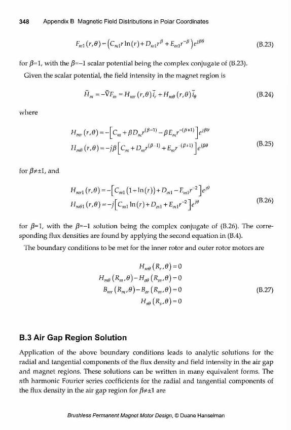
M ) = (Cwirln(r) + Dlulr* +

for with the /3=-l scalar potential being the complex conjugate of (B.23).

Given the scalar potential, the field intensity in the magnet region is

(B.23)

Hm=-VFm=Hmr(r,d)ir + Hme(r/d)le (B.24)

where

(B.25)

for and

H m r l (r,0) = - [ c w l (l + ln(r)) + D m l -E m l r"" 2 ]e '

H m 0 1 (r,0) = - ; [ c m l ln(r) + D m l + E ^ r " 2 ] * ' 6 (B.26)

for /3=1, with the j8=-l solution being the complex conjugate of (B.26). The corre-sponding flux densities are found by applying the second equation in (B.4).

The boundary conditions to be met for the inner rotor and outer rotor motors are

Hm0(Rr,e) = 0

Hm0{Rm,d)-Hntì(Rm,d) = 0

B„ir(Rm/G)-Bar(Rm,e) = 0

Ha9(R5,d) = 0 (B.27)

B.3 Air Gap Region Solution

Application of the above boundary conditions leads to analytic solutions for the radial and tangential components of the flux density and field intensity in the air gap and magnet regions. These solutions can be written in many equivalent forms. The nth harmonic Fourier series coefficients for the radial and tangential components of the flux density in the air gap region for are

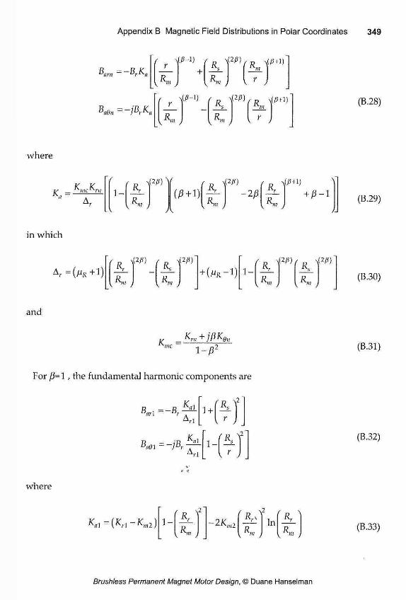
5 _ D ¡X •'arn Drr^a

Badn

/ \

r ~R

R„

(P-1) (Rs)

(20) (R \

K J < r ,

M (20) (R

in I { R * J ^ J

(B.28)

where

K K ^ _ IKmclKrn 1 - A

\(20) / „ \

(iS + l) _Rr

(20) / — \

2/3 A (0+1)

+ /3-1 (B.29)

in which

Rr ^ (20) (20)

1 - A R„.

(2f)) f \(2p) s

(B.30)

and

Kmc Krn +jpKe„

I - / ? 2 (B.31)

For ¡5= 1 , the fundamental harmonic components are

1 - ~°r

}ntí\

Ki \i " Í

Kii 1 - i i 1 -r

\

t-

\2 (B.32)

where

1 -r Rr > ¿ /

RrK I R

r In r Is-J (B.33)

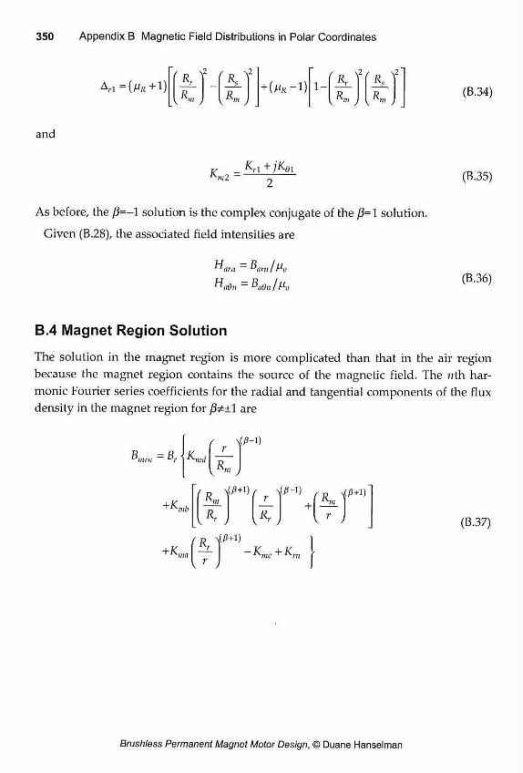
A R..

A R.,

A R,„

A R,„

(B.34)

and

Nirt ~ (B.35)

As before, the solution is the complex conjugate of the p=i solution.

Given (B.28), the associated field intensities are

Harn = B am I Mo HaOn - B(t0n /Mo (B.36)

B.4 Magnet Region Solution

The solution in the magnet region is more complicated than that in the air region because the magnet region contains the source of the magnetic field. The nth har-monic Fourier series coefficients for the radial and tangential components of the flux density in the magnet region for are

K md

/ \(0~D r J n i /

+K mb Ku

(0+1) (0-1)

R \ • /

+K, Rr - Kmc + Km

\(0+1)

(B.37)

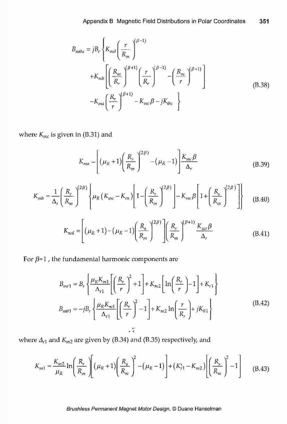
Bm0n - ÌBr 1 K nui V /

+K mb

(0+1) / \ r (/j-i) / n \(/*+D~ in I

U J rT v y

U J -K, - Kmcß ~ iKt)n

(B.38)

where Kmc is given in (B.31) and

(Mr+1) K — ^ma

- ( m r - 1 ) Kncß

nb 1 (Rr)

(2/3)

A, l^J Vr{Kwc~K 1 - A

R„

\(2ß)

-Kncß 1 + A R„

(2/J)

Kmd ~ ( O 2/3)

M K A

For ß=l, the fundamental harmonic components are

mrl 1 ^x

5 _ j D MRKml m01 - ~] r

R r i r

rR

+1 + K

T VI - 7 1 - 1

m2

+ K,„2ln

lnl — 1-1 + K,

/

r v * ,

+ Ä 1

where Ar-\ and Km2 are given by (B.34) and (B.35) respectively, and

Mr v*» , (Mr+1)

Re \2

" (Mr-1) A \ /

- 1

(B.39)

(B.40)

(B.41)

(B.42)

(B.43)

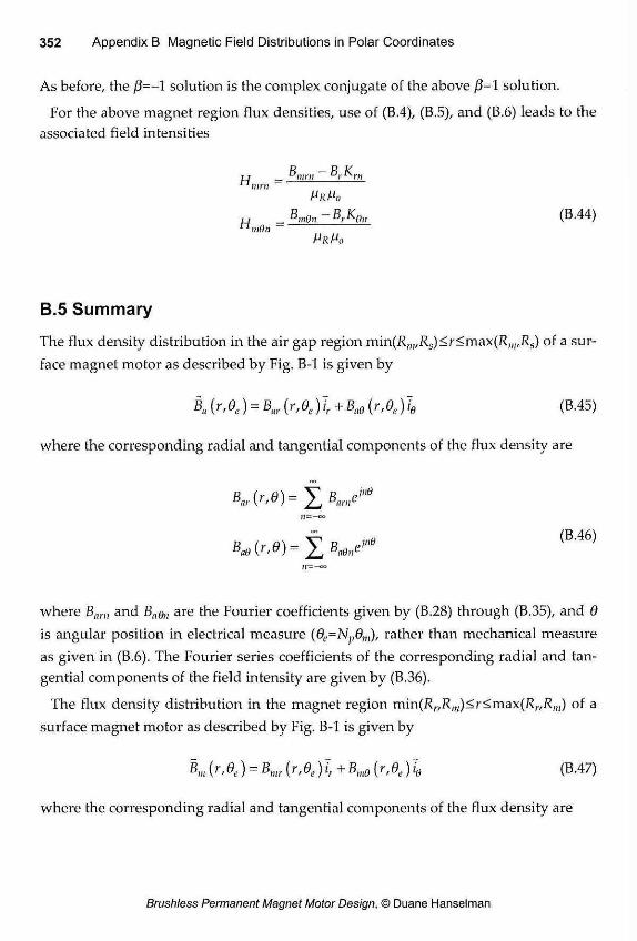
As before, the /3=-l solution is the complex conjugate of the above ¡5=1 solution.

For the above magnet region flux densities, use of (B.4), (B.5), and (B.6) leads to the associated field intensities

d R K tt _ Dmrn DrIsrn n mm

IT _ um0n ur'^0n n mdn -

MRMO

ZMO» ( B - 4 4 ) MR MO

B.5 Summary

The flux density distribution in the air gap region mm(Rm,Rs)<r<max(Rm,Rs) of a sur-face magnet motor as described by Fig. B-l is given by

B« (rA) = B«r (rA)l + Boo ('A-Vo (B.45)

where the corresponding radial and tangential components of the flux density are

Bar(r,6)= £ Bame'"0

BM= i w * * ( B ' 4 6 ) 11=-oo

where B a r n and B ^ are the Fourier coefficients given by (B.28) through (B.35), and 6 is angular position in electrical measure (0e=Np6m), rather than mechanical measure as given in (B.6). The Fourier series coefficients of the corresponding radial and tan-gential components of the field intensity are given by (B.36).

The flux density distribution in the magnet region min(Kr,Rm)<?'^max(R,-,R,H ) of a surface magnet motor as described by Fig. B-l is given by

K (rA) = Kr (rA)l+Ko (rA)h (B.47)

where the corresponding radial and tangential components of the flux density are

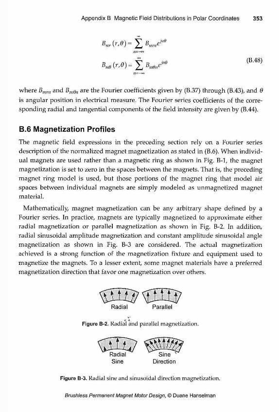
n=-<*>

Bm0 KT'O)- ¿ j Bwdne

n=- oo

where Bnmt and Bu,en are the Fourier coefficients given by (B.37) through (B.43), and 6 is angular position in electrical measure. The Fourier series coefficients of the corre-sponding radial and tangential components of the field intensity are given by (B.44).

B.6 Magnetization Profiles

The magnetic field expressions in the preceding section rely on a Fourier series description of the normalized magnet magnetization as stated in (B.6). When individ-ual magnets are used rather than a magnetic ring as shown in Fig. B-l, the magnet magnetization is set to zero in the spaces between the magnets. That is, the preceding magnet ring model is used, but those portions of the magnet ring that model air spaces between individual magnets are simply modeled as unmagnetized magnet material.

Mathematically, magnet magnetization can be any arbitrary shape defined by a Fourier series. In practice, magnets are typically magnetized to approximate either radial magnetization or parallel magnetization as shown in Fig. B-2. In addition, radial sinusoidal amplitude magnetization and constant amplitude sinusoidal angle magnetization as shown in Fig. B-3 are considered. The actual magnetization achieved is a strong function of the magnetization fixture and equipment used to magnetize the magnets. To a lesser extent, some magnet materials have a preferred magnetization direction that favor one magnetization over others.

Radial Parallel

* <ï Figure B-2. Radial and parallel magnetization.

Sine Direction

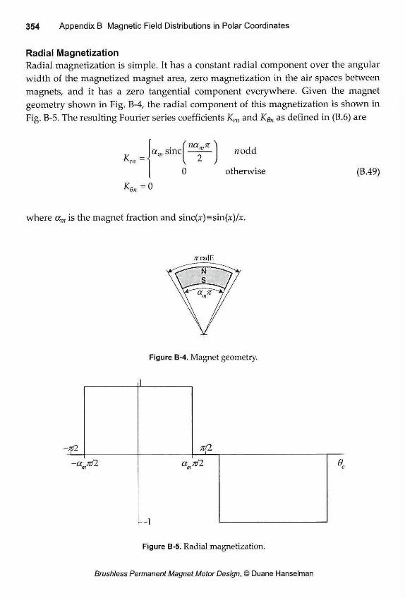
Radial Magnetization Radial magnetization is simple. It has a constant radial component over the angular width of the magnetized magnet area, zero magnetization in the air spaces between magnets, and it has a zero tangential component everywhere. Given the magnet geometry shown in Fig. B-4, the radial component of this magnetization is shown in Fig. B-5. The resulting Fourier series coefficients Krn and as defined in (B.6) are

nodd

0 otherwise (B.49)

where a,,, is the magnet fraction and sinc(x)=sin(x)/x.

;r radE

Figure B-4. Magnet geometry.

-nil d, c

Figure B-5. Radial magnetization.

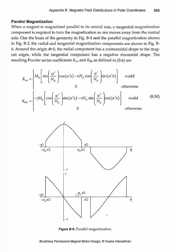
Parallel Magnetization When a magnet is magnetized parallel to its central axis, a tangential magnetization component is required to turn the magnetization as one moves away from the central axis. One the basis of the geometry in Fig. B-4 and the parallel magnetization shown in Fig. B-2, the radial and tangential magnetization components are shown in Fig. B-6. Around the origin 0=0, the radial component has a cosinusoidal shape to the mag-net edges, while the tangential component has a negative sinusoidal shape. The resulting Fourier series coefficients Krn and Kq,j as defined in (B.6) are

/ \

Mv sin a' p

\

K-dn ~ -jMf

/ \

cr\ c a LUJ

i ^ J

cos(a'n)-nNp cos

0

sin.(a'n)-nNp sin

0

, > a sin (a'n) sin (a'n) p J

a AL

cos(a'n)

?zodd

otherwise

n odd

otherwise

(B.50)

7t2

i

nil -amnl2

--1

r/2 (9,

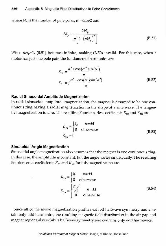
356 Appendix B Magnetic Field Distributions in Polar Coordinates

where Np is the number of pole pairs, a'=amJt/2 and

2N„

l-(NNpJ (B.51)

When nNp= 1, (B.51) becomes infinite, making (B.50) invalid. For this case, when a motor has just one pole pair, the fundamental harmonics are

a ' +cos (a') sin (a') KRL =

. a '-cos(a')sin (a') (B.52) Ko l =]

Radial Sinusoidal Amplitude Magnetization In radial sinusoidal amplitude magnetization, the magnet is assumed to be one con-tinuous ring having a radial magnetization in the shape of a sine wave. The tangen-tial magnetization is zero. The resulting Fourier series coefficients KRN and K^ are

—

/ 2 ii=± 1

0 otherwise

Ke«= 0 (B.53)

Sinusoidal Angle Magnetization Sinusoidal angle magnetization also assumes that the magnet is one continuous ring. In this case, the amplitude is constant, but the angle varies sinusoidally. The resulting Fourier series coefficients KRN and Kq,, for this magnetization are

K,.„ — YL N = ±L 0 otherwise

0 otherwise

Since all of the above magnetization profiles exhibit halfwave symmetry and con-tain only odd harmonics, the resulting magnetic field distribution in the air gap and magnet regions also exhibits halfwave symmetry and contains only odd harmonics.

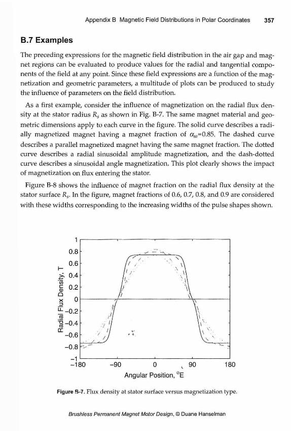
The preceding expressions for the magnetic field distribution in the air gap and mag-net regions can be evaluated to produce values for the radial and tangential compo-nents of the field at any point. Since these field expressions are a function of the mag-netization and geometric parameters, a multitude of plots can be produced to study the influence of parameters on the field distribution.

As a first example, consider the influence of magnetization on the radial flux den-sity at the stator radius Rs as shown in Fig. B-7. The same magnet material and geo-metric dimensions apply to each curve in the figure. The solid curve describes a radi-ally magnetized magnet having a magnet fraction of a„,=0.85. The dashed curve describes a parallel magnetized magnet having the same magnet fraction. The dotted curve describes a radial sinusoidal amplitude magnetization, and the dash-dotted curve describes a sinusoidal angle magnetization. This plot clearly shows the impact of magnetization on flux entering the stator.

Figure B-8 shows the influence of magnet fraction on the radial flux density at the stator surface Rs. In the figure, magnet fractions of 0.6, 0.7, 0.8, and 0.9 are considered with these widths corresponding to the increasing widths of the pulse shapes shown.

- 1 - 1 8 0 -90 0 , 90

Angular Position, °E

Figure 5-7. Flux density at stator surface versus magnetization type.

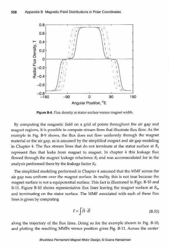
0 .8

- 0 . 8 L -- 1 8 0 -90 0

Angular Position, °E 90 180

Figure B-8. Flux density at stator surface versus magnet width.

By computing the magnetic field on a grid of points throughout the air gap and magnet regions, it is possible to compute stream lines that illustrate flux flow. As the example in Fig. B-9 shows, the flux does not flow uniformly through the magnet material or the air gap, as is assumed by the simplified magnet and air gap modeling in Chapter 4. The flux stream lines that do not terminate at the stator surface at Rs

represent flux that leaks from magnet to magnet. In chapter 4 this leakage flux flowed through the magnet leakage reluctance R/ and was accommodated for in the analysis performed there by the leakage factor Kj.

The simplified modeling performed in Chapter 4 assumed that the MMF across the air gap was uniform over the magnet surface. In reality, this is not true because the magnet surface is not a equipotential surface. This fact is illustrated in Figs. B-10 and B-ll. Figure B-10 shows representative flux lines leaving the magnet surface at Rm

and terminating on the stator surface. The MMF associated with each of these flux lines is given by computing

along the trajectory of the flux lines. Doing so for the example shown in Fig. B-10, and plotting the resulting MMFs versus position gives Fig. B-ll . Across the center

(B.55)

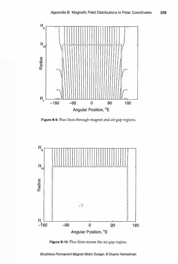
r - 1 8 0 - 9 0 0 90 180

Angular Position, °E

Figure B-9. Flux lines through magnet and air gap regions.

Angular Position, °E

Figure B-10. Flux lines across the air gap region.

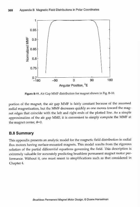
1

0.95

~o | 0.85 CO E

| 0.8

0.75

0.7 -180 -90 0 90 180

Angular Position, °E

Figure B-11. Air Gap MMF distribution for magnet shown in Fig. B-10.

portion of the magnet, the air gap MMF is fairly constant because of the assumed radial magnetization, but the MMF decreases quickly as one moves toward the mag-net edges that coincide with the left and right ends of the plotted line. As a simple approximation of the air gap MMF, it is convenient to simply compute the MMF at the magnet center, 0=0.

B.8 Summary

This appendix presents an analytic model for the magnetic field distribution in radial flux motors having surface-mounted magnets. This model results from the rigorous solution of the partial differential equations governing the field. This description is extremely valuable for accurately predicting brushless permanent magnet motor per-formance. Without it, one must resort to simplifications such as that considered in Chapter 4.

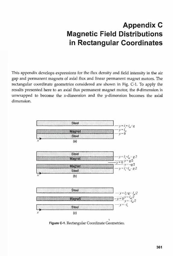
Appendix C Magnetic Field Distributions in Rectangular Coordinates

This appendix develops expressions for the flux density and field intensity in the air gap and permanent magnets of axial flux and linear permanent magnet motors. The rectangular coordinate geometries considered are shown in Fig. C-l. To apply the results presented here to an axial flux permanent magnet motor, the ^-dimension is unwrapped to become the x-dimension and the y-dimension becomes the axial dimension.

- 3-=/=r /,,/-7

, V = 1/2

— v = -/v

(c)

Figure C-1. Rectangular Coordinate Geometries.

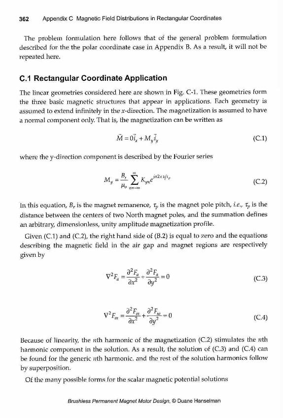
The problem formulation here follows that of the general problem formulation described for the the polar coordinate case in Appendix B. As a result, it will not be repeated here.

C.1 Rectangular Coordinate Application

The linear geometries considered here are shown in Fig. C-l. These geometries form the three basic magnetic structures that appear in applications. Each geometry is assumed to extend infinitely in the x-direction. The magnetization is assumed to have a normal component only. That is, the magnetization can be written as

M = 0lx+Myiy (C.l)

where the y-direction component is described by the Fourier series

(C.2) r*0 K=—oo

In this equation, Br is the magnet remanence, rp is the magnet pole pitch, i.e., Tp is the distance between the centers of two North magnet poles, and the summation defines an arbitrary, dimensionless, unity amplitude magnetization profile.

Given (C.l) and (C.2), the right hand side of (B.2) is equal to zero and the equations describing the magnetic field in the air gap and magnet regions are respectively given by

V 2 F + = 0 (r fl dx2 dy2 ( C 3 )

y2p _ d2Fm d2Fm V f ' » - a*2 + 3 / ( C 4 >

Because of linearity, the nth harmonic of the magnetization (C.2) stimulates the nth harmonic component in the solution. As a result, the solution of (C.3) and (C.4) can be found for the generic nth harmonic, and the rest of the solution harmonics follow by superposition.

Of the many possible forms for the scalar magnetic potential solutions

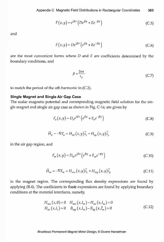
F(X/y) = e'lix ( D / v + Ee~fiv) (C.5)

and

F{xfy) = De'f,x(e^ + Ee~^) (C.6)

are the most convenient forms where D and £ are coefficients determined by the boundary conditions, and

b-^L ~ (C-7)

to match the period of the nth harmonic in (C.2).

Single Magnet and Single Air Gap Case The scalar magnetic potential and corresponding magnetic field solution for the sin-gle magnet and single air gap case as shown in Fig. C-lfl, are given by

= + (C.8)

Ha = ~VFfl = Hax {x,y)lx+ Hay (x,y) iy (C.9)

in the air gap region, and

=-VF„, = Hmx (x,y)I + Hmy (x,y)ly (C.ll)

in the magnet region. The corresponding flux density expressions are found by applying (B.4). The coefficients in thes£ expressions are found by applying boundary conditions at the material interfaces, namely,

Hmx (x,0) = 0 Hmx (x,lm ) - Hax (x,lm ) = 0 Hax (x,ls ) = 0 Bmy (x,lm ) - Bay (x,tm ) = 0 ( C " 1 2 )

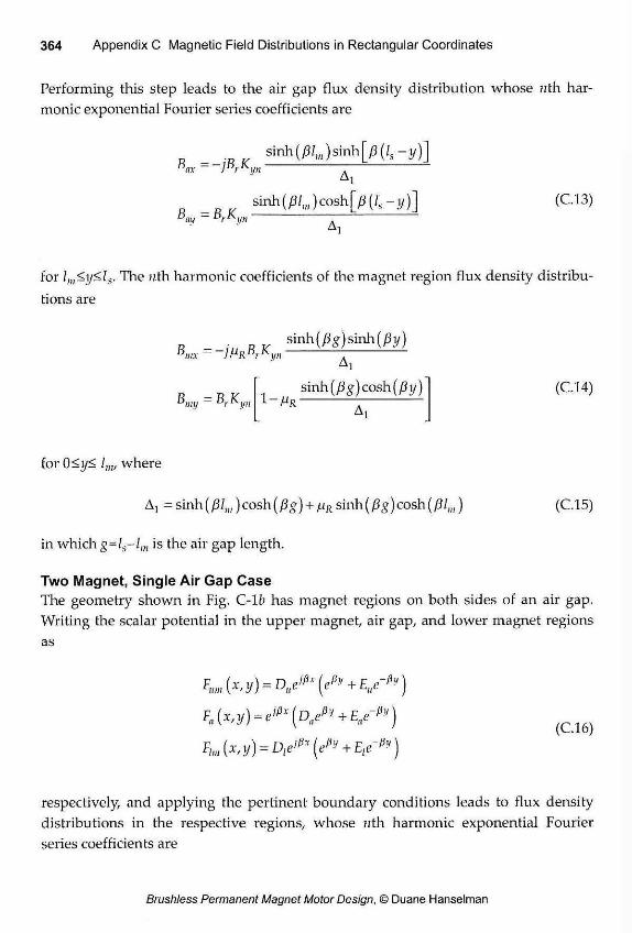
Performing this step leads to the air gap flux density distribution whose /ith har-monic exponential Fourier series coefficients are

sinh(/3/,„)sinh[/?(/s -i/)] "ax ~ -J°rKyn 7

A 1 sinh(j3/w)cosh[/J(/s-y)] (C.13)

Bay - BrKyn Ai

for lln<y<ls. The nth harmonic coefficients of the magnet region flux density distribu-tions are

sinh(lg)sinh(/3y) nix ~ i

1 _ D v 'my r i/n 1 - M r

A]

sinh(ßg)cosh(ßy) (C.14)

for 0<i/< /,„, where

A, =smh(ßlvl)cosh(ßg) + vRsinh(ßg)cosh(ßlm) (C.15)

in which g=ls-lm is the air gap length.

Two Magnet, Single Air Gap Case The geometry shown in Fig. C-lb has magnet regions on both sides of an air gap. Writing the scalar potential in the upper magnet, air gap, and lower magnet regions

+ ( c i 6 )

respectively, and applying the pertinent boundary conditions leads to flux density distributions in the respective regions, whose nth harmonic exponential Fourier series coefficients are

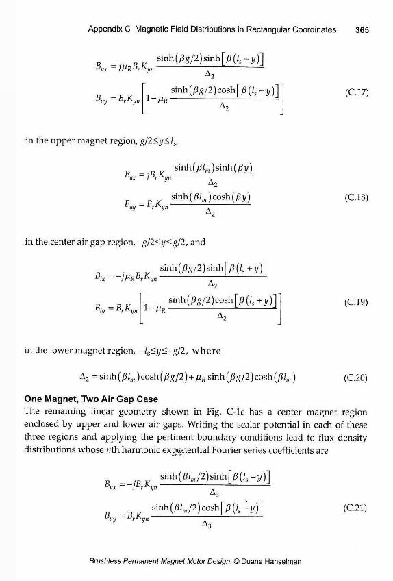
. sinh(^/2)sinh[y3(/s-y)] - )ßRörKv„

2

sinh(/Jg/2)cosh[/J(Zs-y)l ~ Mr ÌUy B r Kyn

(C.l 7)

in the upper magnet region, g/2<y<ls,

Bax =ÌBrK

3 _ D 1/ «1/ Dr yn

sivh(ßlm ) sinh (ßy) A2

sinh(ßlm ) cosh (ßy) (C.l 8)

in the center air gap region, -g/2<y<g/2, and

sinh(/^/2)sinh[/?(/s+y)] B , x = ')Mrb^ un

ìly - BrKl/n 1-Mr sinh(jgg/2)cosh[/î (f s+y)]

A, (C.19)

in the lower magnet region, -ls<y<-g/2, where

A2 = sinh (film ) cosh (0g/2) + nR sinh (fig/2) cosh (fil,H ) (C.20)

One Magnet, Two Air Gap Case The remaining linear geometry shown in Fig. C-lc has a center magnet region enclosed by upper and lower air gaps. Writing the scalar potential in each of these three regions and applying the pertinent boundary conditions lead to flux density distributions whose ?zth harmonic exponential Fourier series coefficients are

BuX=-ßrK sinh(/5/,„/2)sinh[/3(/s-y)]

yn Ac

? _ D y ity DrIKyn sinh (/?/„,/2) cosh [ß(/s - y ) ] (C.21)

A,

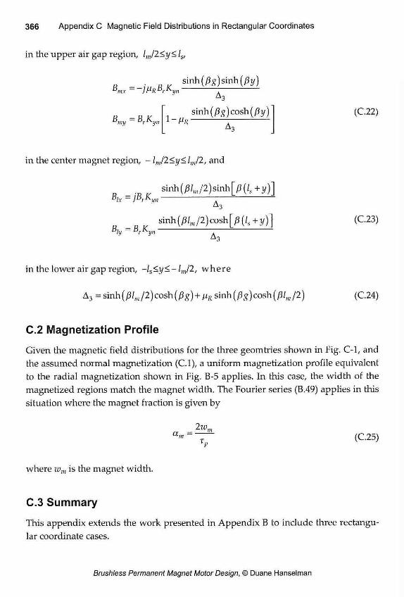
366 Appendix C Magnetic Field Distributions in Rectangular Coordinates

in the upper air gap region, lm/2<y<

n n y Sinh(/?g)sinh(/3y) bmx = -)^RbrKyn 7

A 3 sinh (fig) cosh (py) J _ D j/

'my Dr yn 1 " Vii

in the center magnet region, - lm/2<y<lm/2, and

sinh(/3/,„/2)sinh [jB(/s+y)] Bix - jBrK V" A

(C.22)

smh(ßlm/2)cosh[ß(ls + y)] (C.23) Bly - BrKyn

in the lower air gap region, -ls<y<-lm/2, where

A3 = sinh(/?/,„/2)cosh + sinh (/3g)cosh(/}/m/2) (C.24)

C.2 Magnetization Profile

Given the magnetic field distributions for the three geomtries shown in Fig. C-l, and the assumed normal magnetization (C.l), a uniform magnetization profile equivalent to the radial magnetization shown in Fig. B-5 applies. In this case, the width of the magnetized regions match the magnet width. The Fourier series (B.49) applies in this situation where the magnet fraction is given by

_ 2wm a " ' ~ (C.25) xv

where wm is the magnet width.

C.3 Summary

This appendix extends the work presented in Appendix B to include three rectangu-lar coordinate cases.

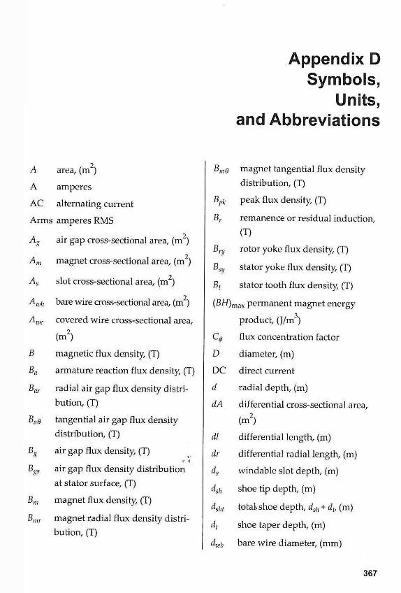
Appendix D Symbols,

Units, and Abbreviations

A area, (m2)

A amperes

AC alternating current

Arms amperes RMS

Ar air gap cross-sectional area, (m )

Am magnet cross-sectional area, (m )

As slot cross-sectional area, (m )

Awb bare wire cross-sectional area, (m )

Awc covered wire cross-sectional area,

(m2)

B magnetic flux density, (T)

Ba armature reaction flux density, (T) Bar radial air gap flux density distri-

bution, (T)

Bae tangential air gap flux density distribution, (T)

Bg air gap flux density, (T) * "

BgS air gap flux density distribution

at stator surface, (T)

Bm magnet flux density, (T) Bmr magnet radial flux density distri-

bution, (T)

Bwd magnet tangential flux density

distribution, (T)

Bpk peak flux density, (T) Br remanence or residual induction,

(T)

Bry rotor yoke flux density, (T)

Bsy s ta tor yoke fl ux densi ty, (T)

Bt stator tooth flux density, (T)

(BH)m a x permanent magnet energy

product, (J/m3)

Q flux concentration factor

D diameter, (m)

DC direct current

d radial depth, (m)

dA differential cross-sectional area,

(m2)

dl differential length, (m)

dr differential radial length, (m)

ds windable slot depth, (m)

dsh shoe tip depth, (m)

dsht total shoe depth, dsh + dlr (m)

dt shoe taper depth, (m)

dwi, bare wire diameter, (mm)

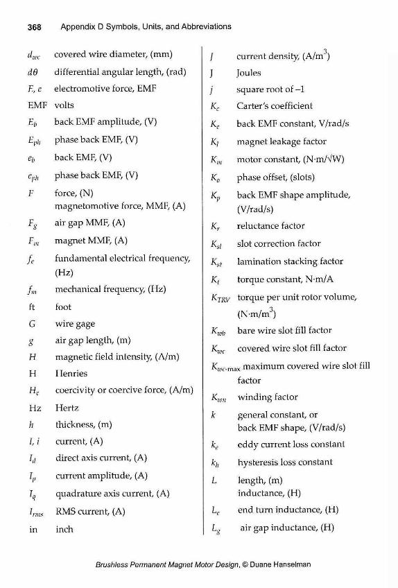
djvc covered wire diameter, (mm)

de differential angular length, (rad)

E,c electromotive force, EMF

EMF volts

Eb back EMF amplitude, (V)

Eph phase back EMF, (V)

tb back EMF, (V)

eph phase back EMF, (V)

F force, (N) magnetomotive force, MMF, (A)

air gap MMF, (A)

F,n magnet MMF, (A)

fc fundamental electrical frequency, (Hz)

fm mechanical frequency, (Hz)

ft foot

G wire gage

8 air gap length, (m)

H magnetic field intensity, (A/m)

H Henries

Hc coercivity or coercive force, (A/m)

Hz Hertz

h thickness, (m)

1, i current, (A)

h direct axis current, (A)

h current amplitude, (A)

quadrature axis current, (A)

Lins RMS current, (A)

in inch

/ 3 current density, (A/m")

J Joules

i square root of -1

Kc Carter's coefficient

Kc back EMF constant, V/rad/s

K, magnet leakage factor

Kn motor constant, (N-m/VW)

K0 phase offset, (slots)

Kp back EMF shape amplitude, (V/rad/s)

Kr reluctance factor

Ks, slot correction factor

Kst lamination stacking factor

Kt torque constant, N-m/A

Ktrv torque per unit rotor volume,

(N-m/m3)

Kwb bare wire slot fill factor

Koc covered wire slot fill factor

Koc-max maximum covered wire slot factor

K-wn winding factor

k general constant, or back EMF shape, (V/rad/s)

K eddy current loss constant

h hysteresis loss constant

L length, (m) inductance, (H)

K end turn inductance, (H)

air gap inductance, (H)

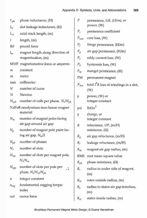
Lph phase inductance, (H) P permeance, 1/R, (H/m), or

Ls slot leakage inductance, (H) power, (W)

Ls, axial stack length, (m) Pc permeance coefficient

I length, (m) P 1 core

core loss, (W)

Ibf pound force P f fringe permeance, (H/m)

l,n magnet length along direction of PS

air gap permeance, (H/m)

magnetization, (m) Pc eddy current loss, (W)

MMF magnetomotive force or amperes Ph hysteresis loss, (W) m constant Pm manget permeance, (H) m meter PM permanent magnet mm millimeter 2 mm millimeter

Pslot total I R loss of windings in a slot, N number of turns (W) N Newton

V power, (W) or K-ph number of coils per phase, NJN^ integer constant

NdFeB neodymium-iron-boron magnet psi lbf/in2

material <? charge, or

Nm number of magnet poles facing integer constant air gap around air gap R reluctance, 1/P, (m/H)

Np number of magnet pole pairs fac- resistance, (Q) ing air gap, NJ2

RS air gap reluctance, (m/H)

Mph number of phases R¡ leakage reluctance, (m/H)

K number of slots Rm magnet-air gap radius, (m)

Km number of slots per magnet pole, RMS root mean square value NJNm

Rph phase resistance, (O) N w number of slots per pole per

* *

phase, NJNJNph

Rr radius to under side of magnet, (m)

n integer constant Ryo rotor outside radius, (m)

fundamental cogging torque Rs radius to stator-air gap interface,

index radius to stator-air gap interface,

index (m)

ozf ounce force Rsi stator inside radius, (m)

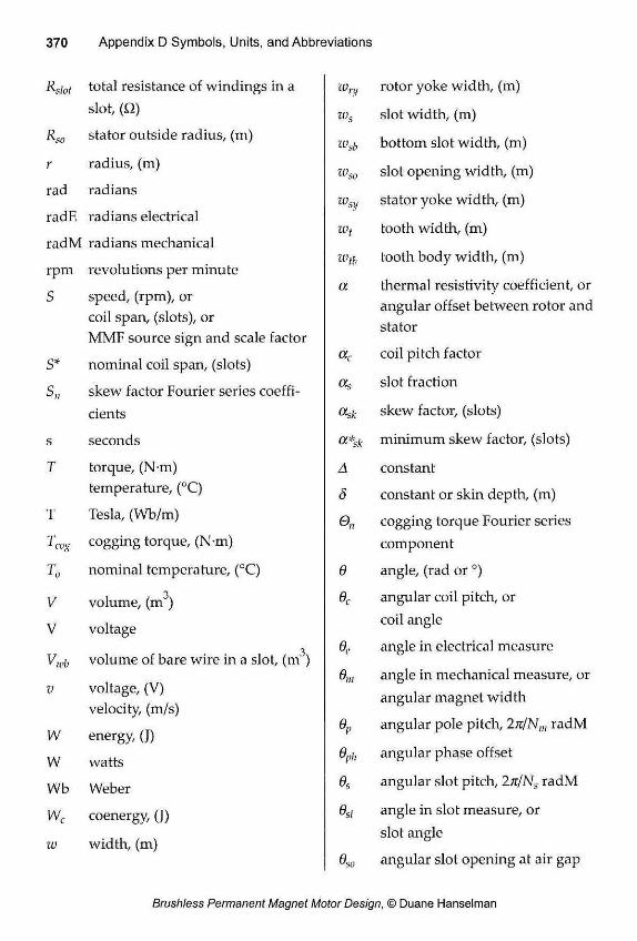
Rslot total resistance of windings in a slot, (Q)

Rso stator outside radius, (m)

r radius, (m)

rad radians

radE radians electrical

radM radians mechanical

rpm revolutions per minute

S speed, (rpm), or coil span, (slots), or MMF source sign and scale factor

S* nominal coil span, (slots) S„ skew factor Fourier series coeffi-

cients

s seconds

T torque, (N-m)

temperature, (°C)

T Tesla, (Wb/m) Tcog cogging torque, (N-m)

T0 nominal temperature, (°C) 3

V volume, (m ) V voltage

Vu,b volume of bare wire in a slot, (m3)

v voltage, (V) velocity, (m/s)

W energy, (J)

W watts

Wb Weber

Wc coenergy, (J)

w width, (m)

Wry rotor yoke width, (m)

Ws slot width, (m)

Wsb bottom slot width, (m)

Wso slot opening width, (m)

W$y stator yoke width, (m)

Wt tooth width, (m)

Wtb tooth body width, (m)

a thermal resistivity coefficient, or angular offset between rotor and stator

CCc coil pitch factor

as slot fraction

ask skew factor, (slots)

a * s k minimum skew factor, (slots)

A constant

Ö constant or skin depth, (m)

cogging torque Fourier series component

e angle, (rad or °)

Oc angular coil pitch, or coil angle

Oc angle in electrical measure

Oui angle in mechanical measure, or angular magnet width

e„ angular pole pitch, In/bl,„ radM

Oph angular phase offset

0s angular slot pitch, 2 x / N s radM

Osi angle in slot measure, or slot angle

Oso angular slot opening at air gap

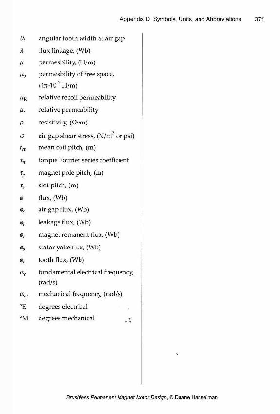
0t angular tooth width at air gap

A, flux linkage, (Wb)

M permeability, (H/m)

Mo permeability of free space,

(471-10"7 H/m)

MR relative recoil permeability

Mr relative permeability

P resistivity, (Q-m)

G 2 air gap shear stress, (N/m or psi)

tcp mean coil pitch, (m)

torque Fourier series coefficient

Tp magnet pole pitch, (m)

% slot pitch, (m)

<t> flux, (Wb)

air gap flux, (Wb)

<t>l leakage flux, (Wb)

<Pr magnet remanent flux, (Wb)

<Ps stator yoke flux, (Wb)

<Pt tooth flux, (Wb)

C0e fundamental electrical frequency, (rad/s)

Olm mechanical frequency, (rad/s)

°E degrees electrical

°M degrees mechanical

Appendix E Glossary

This appendix defines terms used in describing brushless permanent magnet motors. Each term appears in italics where it is first used.

air gap: the air space between the rotor and stator of a motor.

air gap inductance: winding inductance due to flux crossing an air gap.

alignment torque: torque produced by the interaction of the magnetic fields produced by permanent magnets and winding currents, also called mutual torque.

Ampere's law: a fundamental law describing a magnetic field created by a current.

armature reaction: magnetic field produced by motor windings as opposed to the mag-netic field produced by permanent magnets.

B-H curve: a plot of the flux density versus field intensity for a nonlinear material.

back EMF: voltage produced in a winding due to permanent magnet motion.

back EMF constant: the rate at which back EMF increases with speed.

balanced winding: motor windings that produce back EMFs having the same ampli-tude and shape, and the relative phase offset between each back EMF is 120°E for three phase motors.

BLi law: force produced by the interaction of a magnetic field and current in a wire over a length L.

BLv law: back EMF produced by the-mteraction of a magnetic field moving past a wire at a velocity v.

breadloaf: magnet cross-sectional shape that resembles the shape of bread baked in a loaf pan where the bottom and sides of the magnet are flat and the top facing the air gap is curved.

Carter's coefficient: a factor that specifies how much an air gap must be increased ana-lytically to take into account the presence of slots.

chorded: a short-pitched coil or winding.

coercivity or coercive force, Hc: field intensity across a permanent magnet when the space between the North and South poles has zero permeance.

cogging torque: torque produced by permanent magnets seeking maximum alignment with stator teeth.

coil pitch: angular span or spread of a coil.

coil pitch factor: ratio of coil pitch to pole pitch.

commutation: the process of successively energizing and denergizing motor phase windings in a way that produces useful torque.

commutation torque ripple: torque ripple created by imperfect motor commutation.

concentrated or solenoidal windings: windings that are physically isolated from other phase windings.

copper motor: motor construction that maximizes space for windings.

core: a shaped structure of ferromagnetic material that conducts magnetic flux.

core losses: combined hysteresis and eddy current losses in a material.

demagnetization curve: relationship between flux density and field intensity for a per-manent magnet after it has been magnetized.

detent position: rotor position where there is zero torque.

distributed windings: windings that are distributed and interlaced with other phase windings.

double layer winding: a motor winding where two coil sides appear in every motor slot.

eddy currents: currents induced in electrically conducting material by a changing magnetic field, produces energy loss in the material.

eddy current losses: energy losses due to eddy currents.

electromotive force: EMF, voltage.

end turns: coil turns that extend beyond the stator slots.

end turn inductance: winding inductance due to coil end turns.

Faraday's law: the relationship between the flux linked to a coil and the voltage appearing across its terminals.

ferromagnetic material: material such as steel that is highly permeable to magnetic fields.

field intensity: the force that moves the magnetic field fluid flux density, a spatial vec-tor quantity.

finite element analysis: numerical solution of magnetic field problems that

flux: magnetic field fluid, a scalar quantity describing the net fluid passing through an area.

flux concentration factor: amount by which air gap flux density is greater than that of a permanent magnet providing the air gap flux.

flux linkage: the total flux linked by a winding.

flux density: the density of the magnetic field fluid at a point in space, a spatial vector quantity.

fractional pitch magnet: a magnet pole that spans less than 180°E.

fractional pitch winding: a winding composed of coils that span less than 180°E.

fractional slot motor: a motor that does not support full pitch windings.

full pitch winding: a winding composed of coils that span 180 °E.

fundamental electrical frequency: frequency of the back EMF produced in a winding due to rotor motion.

hysteresis: a property of magnetic materials where the flux density in a material is a function of the history of the field intensity across the material, produces energy loss in a material.

hysteresis loops: closed loops formed in the material characteristics of nonlinear mag-netic materials under AC excitation conditions.

t* r *

hysteresis losses: energy losses due to hysteresis.

inside-out motor: motor construction where the stator is inside the rotor.

integral slot motor: a motor that supports full pitch windings. intrinsic demagnetization curve: demagnetization curve of a magnetized permanent

magnet independent of its operating environment.

ironless: a motor that is slotless, but may as well lack stator back iron.

knee: a bend in the second quadrant demagnetization curve of a permanent magnet.

leakage factor: an empirical factor that relates magnet flux to air gap flux.

Lenz's law: defines the polarity of the voltage induced in a coil. The induced voltage will cause a current to flow in a closed circuit in a direction such that its magnetic effect will oppose the change that produces it.

Lorentz force equation: force experienced by a moving charge in the presence of a mag-netic field.

magnet leakage flux: magnet flux that does not cross the air gap into the stator.

magnet leakage permeance: permeance associated with permanent magnet magnetic cir-cuit model.

magnet motor: motor construction that maximizes utilization of permanent magnet material.

magnetic circuit analysis: solution of magnetic field problems using lumped parameter material approximations based on assumptions of magnetic field uniformity and direction.

MMF: magnetomotive force, the sum or net total field intensity that moves flux through a material, a scalar quantity, permeability: a fundamental property of materials.

motor constant: description of torque production efficiency.

moving coil: a linear motor design where the windings move and the permanent mag-nets are stationary.

moving magnet: a linear motor design where the windings remain stationary and the permanent magnets move.

mutual torque: torque produced by the interaction of the magnetic fields produced by permanent magnets and winding currents, also called alignment torque.

normal demagnetization curve: demagnetization curve of a permanent magnet in a magnetic circuit after it has been magnetized.

ohmic loss or I R loss: energy loss due to nonzero electrical resistance.

pancake motor: an axial flux motor having radially-directed windings.

permeability: a material property that describes how easily magnetic field flows through the material, analogous to how conductivity describes how easily current flows through a material.

permeance: relationship between flux and MMF for a block of material, analogous to electrical conductance.

permeance coefficient: operating point of a permanent magnet in a magnetic circuit.

phase: a motor winding that has a known angular relationship with respect to other phases.

phase offset: the number of slots that the coils of one phase winding are shifted relative to those of the next phase.

phase windings: a collection of coils connected together to form a phase.

pitch: measure of length or angle.

pole: a magnetic pole, e.g., a North or South magnetic pole, formed by permanent magnets or energized coils.

pole pair: the combination of one North and one South magnetic pole.

pole pitch: the period or distance between magnet poles, i.e., the distance from the cen-ter of one magnet pole to the center of the next magnet pole having an opposite magnetization direction, can be expressed as a distance or an angular quantity.

proximity effect: a phenomenon whereby current crowds towards the outer surface of a conductor due to an externally-applied magnetic field.

principle angle: an equivalent angle between -180° and 180°.

printed circuit board motor: an axial flux motor where the stator windings are formed and attached to a printed circuit board.

rare earth: refers to the permanent magnets materials samarium-cobalt and neodym-ium-iron-boron, which contain raretearth elements.

r a

recoil: the movement of the B-H curve of a material after it has been magnetized.

relative permeability: the permeability of a material relative to that of air.

relative permeance: a correction factor that modifies the flux density entering the stator in the area of the stator slots.

relative recoil permeability: relative permeability of a permanent magnet along its demagnetization curve.

reluctance: inverse of permeance, analogous to electrical resistance.

reluctance factor: a factor that compensates for the reluctance of ferromagnetic mate-rial in a magnetic circuit.

reluctance torque: torque produced by permanent magnets acting alone, or by winding currents acting alone.

remanence or residual induction, Br: flux density of a permanent magnet when space between the North and South poles has infinite permeance.

right hand rule: used in the application of the Lorentz force equation. If the right hand is held so that the fingers curl from v to B, the extended thumb points in the direction ofF.

right hand screw rule: used in the application of Ampere's law. Positive current is defined as flowing in the direction of the advance of a right hand screw turned in the direction in which the closed path is traversed.

rotor: the rotational structure in a motor.

rotor yoke or back iron: a ring of ferromagnetic material behind the rotor magnets.

saturation: a nonlinear property of ferromagnetic material whereby it becomes increasingly difficult to force additional magnetic flux through the material as the flux level increases.

shoe: stator tooth projection that partially closes stator slots.

six step drive: motor drive utilizing rectangular pulse currents, also called a brushless DC motor drive.

skin depth: the distance over which the current amplitude drops to e~l or about 37% of its value at the conductor outer surface due to the skin effect and proximity effect.

skin effect: a phenomenon whereby current crowds towards the outer surface of a con-ductor due to the magnetic field created by the current.

slot: space between the stator teeth where windings are placed.

slot fraction: the ratio of the slot opening to the slot pitch.

slot leakage inductance: winding inductance due to magnetic field crossing slots from one side to the other.

slot liner, electrical insulationl added to the slot walls to protect stator windings.

slot permeance coefficient: relationship between the slot permeance and the effective slot permeance in the computation of slot leakage inductance.

slot pitch: the period or distance between slots, i.e., the width of one tooth and one slot; can be expressed as a distance or an angular quantity.

speed voltage: back EMF

stacking factor: ratio of ferromagnetic material area to total area.

stator: the stationary structure in a motor.

stator yoke or back iron: a ring of ferromagnetic material in the stator furthest from the air gap.

teeth: ferromagnetic material in the stator that directs magnet flux past stator wind-ings in the slots.

torque: the twisting force experienced by an object due to a tangential force acting at a radius.

torque constant: the rate at which torque increases with respect to current.

torque ripple: torque variations that exist about a constant value.

transformer voltage: voltage induced across an inductor, Ldi/dt.

triplen: harmonic indices that a multiple of three, i.e., triple-«.

vector: a quantity defined by both an amplitude and a direction.

winding: a collection of connected coils.

Bibliography

Books

H. D. Chai, Electromechanical Motion Devices, Prentice Hall, 1998. This college textbook covers basic magnetics, transformers, DC motors, voice coil actuators, step motors, and brushless DC motors. The text is a very readable alter-native to the more common college textbooks, which focus almost entirely on the terminal characteristics of electric machines.

J. F. Gieras and Z, J. Piech, Linear Synchronous Motors: Transportation and Automation Systems, CRC Press, 2000. This text focuses specifically on linear actuators in a number of motor forms, including variable reluctance, switched reluctance, and permanent magnet. It dis-cusses the application of these actuators to a variety of factory automation appli-cations as well as transportation systems such as Maglev and elevators.

B. Hague, The Principles of Electromagnetism Applied to Electrical Machines, Dover Publi-cations, 1962. This text is an unabridged and unaltered republication of the 1929 text entitled Electromagnetic Problems in Electrical Engineering. The text discloses techniques for determining the magnetic field distribution within motors due to the presence of current carrying wires. A great deal of intuitive insight can be found in the text along with some fairly rigorous mathematical derivations.

D. C. Hanselman, Brushless Permanent-Magnet Motor Design, McGraw-Hill, 1994. This is the first edition to the current text.

B. Heller and V. Hamata, Harmonic Effects in Induction Machines, Elsevier Scientific Publishing Company, 1977, This text provides a great deal of valuable information about the analytical deriva-tion of magnetic fields in the air gaps of electric machines, including Carter's work.

J. R. Hendershot and T. J. E. Miller, Design of Brushless Permanent-Magnet Motors, Magna Physics Publications and Oxford Science Publications, 1994. This is the most comprehensive text on the subject available today. The authors relate information gained from decades of expertise in the design of brushless permanent magnet motors. While much of the material is accessible to the com-mon reader, a good deal of the text assumes greater expertise,

T. Kenjo and S. Nagamori, Permanent-Magnet and Brushless DC Motors, Oxford Science Publications, 1985. This text contains a survey of a variety of brushless permanent magnet motors. It addresses motor construction and electronics for specific markets and contains very good figures.

P. C. Krause, O. Wasynczuk, and S. D. Sudhuff, Analysis of Electric Machinery, IEEE Press, 1995. This text does not cover the design of electrical machines, but rather, it covers their analysis based on terminal characteristics. Reference frame theory, i.e., the ^-transformation and its application to motor control are covered.

P. T. Krein, Elements of Power Electronics, Oxford University Press, 1998. Of all the power electronics texts in existence at this time, this text most closely follows the philosophy shared by this text where the reader is not assumed to be an expert before reading the text.

W. Leonhard, Control of Electric Machines, Springer-Verlag, 1985. A classic text on the control of all common motor types.

W. Leonhard, Control of Electric Machines, Springer-Verlag, 1996. Completely revised and enlarged edition of the above classic text. Though the ter-minology used is European, this text contains a wealth of valuable information that is easily understood.

E. Levi and M. Panzer, Electromechanical Power Conversion, Dover Publications, 1974. This text is a second corrected edition of a text by the same name published by McGraw-Hill in 1966. As with the text by B. Hague, this classic text covers funda-mentals not typically found in any modern text.

M. Liwschitz-Garik and C. C. Whipple, Alternating-Current Machines, Second ed., D. Van Nostrand Company, 1961. This text, first published in 1946, is one of the last classic texts on electric machines. It is one that many well-seasoned motor designers have on their book-shelf. The notation and terminology used is antiquated but discernible.

G. McPherson and R. D. Laramore, An Introduction to Electrical Machines and Trans-formers, second edition, John Wiley and Sons, 1990. This is one example of the many college textbooks available in this area. This text is both more readable and more thorough than most.

T. J. E. Miller, Brushless Permanent-Magnet and Reluctance Motor Drives, Oxford Univer-sity Press, 1989. This text is a survey of modern brushless motors. It is very readable but lacks some depth in most areas simply because the text covers so much ground.

S. A. Nasar, Handbook of Electric Machines, McGraw-Hill, 1987. In its time, this text was a very good handbook. It still contains a great deal of use-ful information.

S. A. Nasar, I. Boldea, and L. E. Unnewehr, Permanent Magnet, Reluctance, and Self-Synchronous Motors, CRC Press, 1993. This is the weakest of the survey texts. Besides some fundamental material on per-manent magnets, there is little of any use in the text.

H. C. Roters, Electromagnetic Devices, John Wiley and Sons, 1941. This is a classic text on magnetic circuit modeling. The circular-arc, straight-line approach to permeance modeling is introduced in this text.

S. J. Salon, Finite Element Analysis of Electrical Machines, Kluwer Academic Publishers, 1995. This text is a good first book to read on finite element analysis applied specifically to electric machines.

P. Vas, Sensorless Vector and Direct Torque Control, Oxford University Press, 1998. A comprehensive treatment of modern motor control. This text is unparalleled in both scope and detail.

W. H. Yeadon and A. W. Yeadon, Handbook of Small Electric Motors, McGraw-Hill, 2001. This text is a compilation of material from a number of authors. Much of the material is excerpts from short courses given by the various contributing authors. A wealth of practical manufacturing information and material properties is pro-vided.

Articles

K. Atallah, Z. Q. Zhu, D. Howe, and T. S. Birch, "Armature reaction field and winding inductances of slotless permanent-magnet brushless machines," IEEE Trans. Mag-netics, vol. 34, no. 5, pp. 3737-3744, Sept. 1998.

K. J. Binns and D. W. Shimmin, "Relationship between rated torque and size of per-manent magnet machines," IEE Proc. Electr. Power Appt., vol. 143, no. 6„ pp. 417-422, Nov. 1996.

N. Boules, "Prediction of no-load flux density distribution in permanent magnet machines," IEEE Trans. Industry Appl, vol. IA-30, no. 4, pp. 633-643, May/June 1985.

C. Breton, J. Bartolome, J. A. Benito, G. Tassinario, I. Flotats, C. W. Lui, and B. J. Chalmers, "Influence of machine symmetry on reduction of cogging torque in permanent-magnet brushless motors," IEEE Trans. Magnetics, vol. 36, no. 5, pp. 3819-3823, Sept. 2000.

F. Fiorillo and A. Novikov, "An improved approach to power losses in magnetic lami-nations under nonsinusoidal induction waveform," IEEE Trans. Magnetics, vol. 26, no. 5, pp. 2904-2910, Sept. 1990.

E. P. Furlani, "Computing the field in permanent-magnet axial-field motors," IEEE Trans. Magnetics, vol. 30, no. 5, pp. 3660-3663, Sept. 1994.

D. C. Hanselman, "Minimum torque ripple, maximum efficiency excitation of brush-less permanent magnet motors," IEEE Trans, hid. Electronics, vol. 41, no. 3, pp. 292-300, June 1994.

D. C. Hanselman and William Peake, "Eddy Current Effects in Slot-Bound Conduc-tors," IEE Proc. Electr. Power Appl, vol. 142, no. 2, pp. 131-136, March 1995.

D. C. Hanselman, "Effect of skew, pole count and slot count on brushless motor radial force, cogging torque and back EMF," IEE Proc. Electr. Power Appl, vol. 144, no. 5„ pp. 325-330, Sept. 1997.

D. Hanselman, "Figure of merit: motor constant indicates brushless motor perform-ance," Power Conversion and Intelligent Motion (PCIM), pp. 32-39, Dec. 1998.

D. Howe and Z. Q. Zhu, "The influence of finite element discretisation on the predic-tion of cogging torque in permanent magnet excited motors," IEEE Trans. Magnet-ics, vol. 28, no. 2, pp. 1080-1083, March 1992.

C. C. Hwang and Y. H. Cho, "Effects of leakage flux on magnetic fields in interior permanent magnet synchronous motors," IEEE Trans. Magnetics, vol. 37, no. 4, pp. 3021-3024, July 2001.

U. Kim and D. K. Lieu, "Magnetic field calculation in permanent magnet motors with rotor eccentricity: without slotting effect," IEEE Trans. Magnetics, vol. 34, no. 4, pp. 2243-2252, July 1998.

U. Kim and D. K. Lieu, "Magnetic field calculation in permanent magnet motors with rotor eccentricity: with slotting effect considered," IEEE Trans. Magnetics, vol. 34, no. 4, pp. 2253-2266, July 1998.

J. Li, T. Abdallah, and C. R. Sullivan, "Improved calculation of core loss with nonsi-nusoidal waveforms," Proc. of IEEE IAS Conf, 2001.

T. J. E. Miller and R. Rabinovici, "Back-EMF waveforms and core losses in brushless DC motors," IEE Proc. Electr. Power Appl, vol. 141, no. 3, pp. 144-154, May 1994.

G. Qishan and G. Hongzhan, "Effect of slotting in PM electric machines," Electric Machines and Power Systems, vol. 10, pp. 273-284, 1985.

R. Rabinovici, "Eddy current losses in permanent magnet motors," IEE Proc. Electr. Power Appl, vol. 141, no. 1, pp. 7-11, Jan. 1994.

K. R Rasmussen, "Analytical prediction of magnetic field from surface mounted per-manent magnet motor," Proc. IEEE IEMDC'99, Seattle, WA, pp. 34-36, May 9-12, 1999.

K. F. Rasmussen, J. H. Davies, T. J. E. Miller, M. I. McGilp, and M. Olaru, "Analytical and numerical computation of air-gap magnetic fields in brushless motors with surface permanent magnets," IEEE Trans. Industry Appl., vol. 36, no. 6, pp. 1547-1554, Nov./Dec. 2000.

W. Roshen, "Ferrite core loss for power magnetic components design," IEEE Trans. Magnetics, vol. 27, no. 6, pp. 4407-4415, Nov. 1991.

K. Sitapati and R. Krishnan, "PerfornYance comparisons of radial and axial field per-manent-magnet, brushless machines," IEEE Trans. Industry Appl, vol. 37, no. 5, pp. 1219-1225, Sept./Oct. 2001.

G. Slemon and X. Liu, "Core losses in permanent magnet motors/' IEEE Trans. Mag-netics, vol. 26, no. 5, pp. 1653-1655, Sept. 1990.

J. G. Zhu and V. S. Ramsdon, "Improved formulations for rotational core losses in rotating electric machines/' IEEE Trans. Magnetics, vol. 34, no. 4, pp. 2234-2242, July 1998.

Z. Q. Zhu and D. Howe, "Analytic prediction of the cogging torque in radial-field permanent magnet brushless motors," IEEE Traits. Magnetics, vol. 28, no. 2, pp. 1371-1374, March 1992.

Z. Q. Zhu, D. Howe, E. Bolte, and B. Ackerman, "Instantaneous magnetic field distri-bution in brushless permanent magnet DC motors, Part I: open-circuit field," IEEE Trans. Magnetics, vol. 29, no. 1, pp. 124-135, January 1993.

Z. Q. Zhu, D. Howe, "Instantaneous magnetic field distribution in brushless perma-nent magnet DC motors, Part II: armature reaction field," IEEE Trans. Magnetics, vol. 29, no. 1, pp. 136-142, January 1993.

Z. Q. Zhu, D. Howe, "Instantaneous magnetic field distribution in brushless perma-nent magnet DC motors, Part III: effect of stator slotting," IEEE Trans. Magnetics, vol. 29, no. 1, pp. 143-151, January 1993.

Z. Q. Zhu, D. Howe, E. Bolte, and B. Ackerman, "Instantaneous magnetic field distri-bution in brushless permanent magnet DC motors, Part IV: magnetic field on load," IEEE Trans. Magnetics, vol. 29, no. 1, pp. 124-135, January 1993.

Z. Q. Zhu and D. Howe, "Influence of design parameters on cogging torque in per-manent magnet machines," IEEE Trans. Energy Conv., vol. 15, no. 4, pp. 407-412, Dec. 2000.

Z. Q. Zhu, D. Howe, and C. C. Chan, "Improved analytical model for predicting the magnetic field distribution in brushless permanent-magnet machines," IEEE Trans. Magnetics, vol. 38, no. 1, pp. 229-238, Jan. 2002.

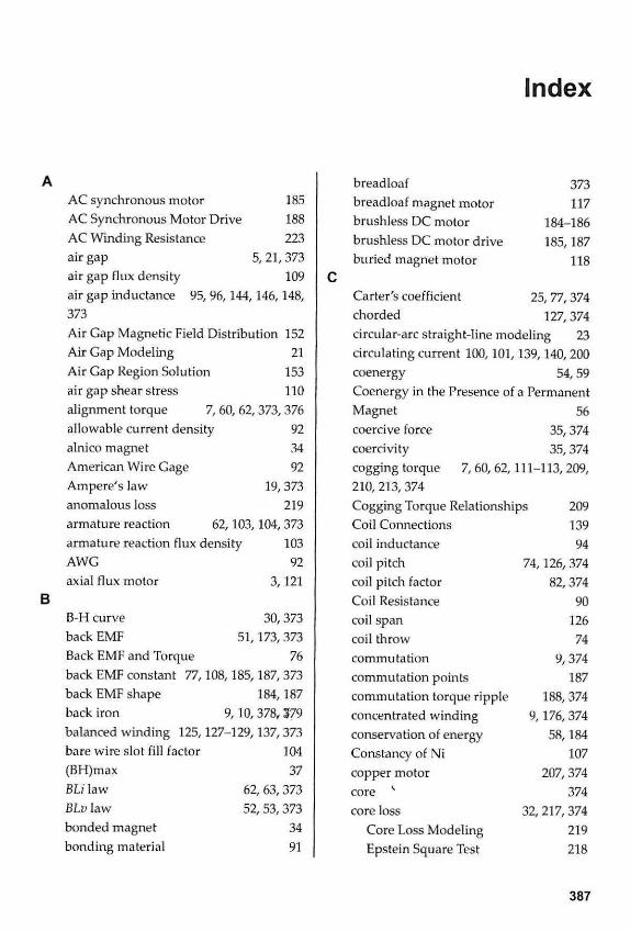
B

AC synchronous motor 185 AC Synchronous Motor Drive 188 AC Winding Resistance 223 air gap 5,21,373 air gap flux density 109 air gap inductance 95, 96,144, 146,148, 373 Air Gap Magnetic Field Distribution 152 Air Gap Modeling 21 Air Gap Region Solution 153 air gap shear stress 110 alignment torque 7, 60, 62,373,376 allowable current density 92 alnico magnet 34 American Wire Gage 92 Ampere's law 19, 373 anomalous loss 219 armature reaction 62, 103,104, 373 armature reaction flux density 103 AWG 92 axial flux motor 3,121

B-H curve 30,373 back EMF 51, 173, 373 Back EMF and Torque 76 back EMF constant 77, 108,185, 187, 373 back EMF shape 184,187 back iron 9,10,378,379 balanced winding 125, 127-129,137, 373 bare wire slot fill factor 104 (BH)max 37 BLi law 62, 63, 373 BLv law 52, 53, 373 bonded magnet 34 bonding material 91

breadloaf 373 breadloaf magnet motor 117 brushless DC motor 184-186 brushless DC motor drive 185,187 buried magnet motor 118

Carter's coefficient 25, 77, 374 chorded 127,374 circular-arc straight-line modeling 23 circulating current 100,101, 139,140,200 coenergy 54,59 Coenergy in the Presence of a Permanent Magnet 56 coercive force 35,374 coercivity 35,374 cogging torque 7, 60, 62,111-113, 209, 210, 213, 374 Cogging Torque Relationships 209 Coil Connections 139 coil inductance 94 coil pitch 74,126, 374 coil pitch factor 82, 374 Coil Resistance 90 coil span 126 coil throw 74 commutation 9,374 commutation points 187 commutation torque ripple 188, 374 concentrated winding 9, 176, 374 conservation of energy 58,184 Constancy of Ni 107 copper motor 207, 374 core v 374 core loss 32, 217, 374

Core Loss Modeling 219 Epstein Square Test 218

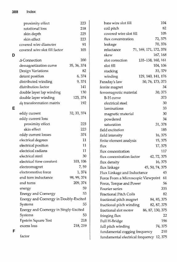
proximity effect 223 rotational loss 218 skin depth 225 skin effect 223

covered wire diameter 91 covered wire slot fill factor 105

4-Connection 200 demagnetization curve 35,36,374 Design Variations 82 detent position 6, 374 distributed winding 9, 374 distribution factor 141 double layer lap winding 130 double layer winding 125, 374 dq transformation matrix 192

eddy current 32, 33, 374 eddy current loss

proximity effect 223 skin effect 223

eddy current losses 374 electrical degrees 11 electrical position 11 electri cal radians 11 electrical steel 30 electrical time constant 103,106 electromagnet 7,59 electromotive force 1, 374 end turn inductance 98, 99, 374 end turns 209, 374 energy 59 Energy and Coenergy 53 Energy and Coenergy in Doubly-Excited Systems 55 Energy and Coenergy in Singly-Excited Systems 53 Epstein Square Test 218 excess loss 218, 219

factor

bare wire slot fill 104 coil pitch 82 covered wire slot fill 105 flux concentration 72,375 leakage 70,376 reluctance 71,169, 171, 172, 378 skew 167,168 slot correction 155-158,160, 161 slot fill 104,106 stacking 33,379 winding 129,140, 141,176

Faraday's law 50, 76, 173, 375 ferrite magnet 34 ferromagnetic material 30, 375

B-H curve 373 electrical steel 30 laminations 33 magnetic material 30 powdered 34 saturation 31,378

field excitation 185 field intensity 16, 375 fini te elem en t a na lysis 15, 375 flux 17,375 flux concentration 117 flux concentration factor 42, 72, 375 flux density 16, 375 flux linkage 45,50, 74, 375 Flux Linkage and Inductance 45 Force From a Microscopic Viewpoint 61 Force, Torque and Power 56 Fourier series 335 Fractional Pitch Coils 82 fractional pitch magnet 84, 85, 375 fractional pitch winding 82, 87, 375 fractional slot motor 86, 87,130, 375 fringing flux 22 Full H-Bridge 196 full pitch winding 74,375 fundamental cogging frequency 210 fundamental electrical frequency 12,375

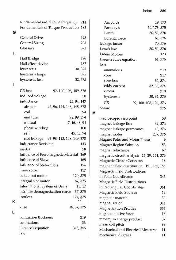
fundamental radial force frequency 214 Fundamentals of Torque Production 183

General Drive General Sizing Glossary

Half Bridge Hall effect device hysteresis hysteresis loops hysteresis loss

193 203 373

196 187

30, 375 375

32, 375

I R loss Induced voltage inductance

air gap coil end turn mutual phase winding self

92,100, 106, 109, 376 50

45,94,143 95,96,144, 146, 148, 373

94 98, 99, 374

7, 46, 48, 94 100

45, 48, 94 slot leakage 96-98, 113, 148, 149, 378

Inductance Revisited 143 inertia 58 Influence of Ferromagnetic Material 169 Influence of Skew 165 Influence of Stator Slots 154 inner rotor 117 inside-out motor 120,375 integral slot motor 87, 375 International System of Units 13, 17 intrinsic demagnetization curve 37, 375 ironless 124,376

knee

lamination thickness laminations Laplace's equation law

36,37, 376

219 33

343, 346

Ampere's Faraday's Lenz's Lorentz force

leakage factor Lenz's law Linear Motors Lorentz force equation loss

anomalous core core loss eddy current excess hysteresis

19, 373 50, 173, 375 50, 52, 376

61, 376 70, 376

50, 52, 376 123

61, 376

I2R ohmic

219 217

32, 374 32,33, 374

218 30, 32, 375

92,100,106,109, 376 376

M macroscopic viewpoint 58 magnet leakage flux 69, 376 magnet leakage permeance 40, 376 magnet motor 207, 376 Magnet Poles and Motor Phases 9 Magnet Region Solution 153 magnet reluctance 69 magnetic circuit analysis 15, 29,151, 376 Magnetic Circuit Concepts 16 magnetic field distribution 151,152,155 Magnetic Field Distributions in Polar Coordinates 343 Magnetic Field Distributions in Rectangular Coordinates 361 Magnetic Field Sources 19 magnetic material 30 magnetization 344 Magnetization Profiles 353 magnetomotive force 18 maximum energy product 37 mean coil pitch 99 Mechanical and Electrical Measures 11 mechanical degrees 11

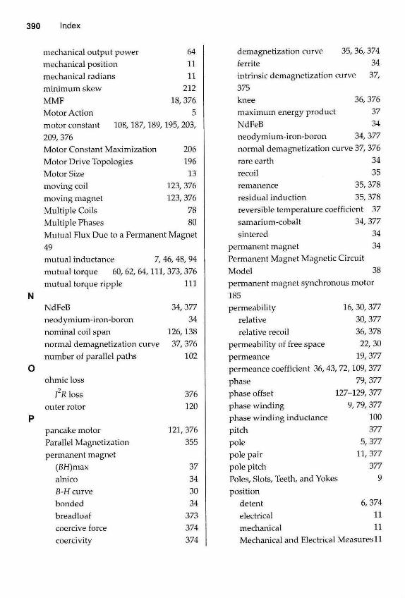
N

mechanical output power 64 mechanical position 11 mechanical radians 11 minimum skew 212 MMF 18,376 Motor Action 5 motor constant 108, 187, 189,195,203, 209,376 Motor Constant Maximization 206 Motor Drive Topologies 196 Motor Size 13 moving coil 123, 376 moving magnet 123,376 Multiple Coils 78 Multiple Phases 80 Mutual Flux Due to a Permanent Magnet 49 mutual inductance 7, 46, 48, 94 mutual torque 60, 62, 64,111, 373, 376 mutual torque ripple 111

NdFeB 34,377 neodymium-iron-boron 34 nominal coil span 126,138 normal demagnetization curve 37,376 number of parallel paths 102

ohmic loss 12R loss

outer rotor

pancake motor Parallel Magnetization permanent magnet

(BH)max alnico B-Hcurve bonded breadloaf coercive force coercivity

376 120

121, 376 355

37 34 30 34

373 374 374

demagnetization curve 35, 36, 374 ferrite 34 intrinsic demagnetization curve 37, 375 knee 36,376 maximum energy product 37 NdFeB 34 neodymium-iron-boron 34,377 normal demagnetization curve 37, 376 rare earth 34 recoil 35 remanence 35,378 residual induction 35, 378 reversible temperature coefficient 37 samarium-cobalt 34,377 sintered 34

permanent magnet 34 Permanent Magnet Magnetic Circuit Model 38 permanent magnet synchronous motor 185 permeability 16, 30, 377

relative 30,377 relative recoil 36, 378

permeability of free space 22, 30 permeance 19,377 permeance coefficient 36,43, 72,109, 377 phase 79,377 phase offset 127-129, 377 phase winding 9, 79, 377 phase winding inductance 100 pitch 377 pole 5,377 pole pair 11, 377 pole pitch 377 Poles, Slots, Teeth, and Yokes 9 position

detent 6,374 electrical H mechanical 11 Mechanical and Electrical Measures 11

Q

position encoder 189 powdered ferromagnetic materials 34 principle angle 377 printed circuit board motor 123, 377 proximity effect 223, 377 psi 110

quadrature 192 quasi-Poisson partial differential equa-tion 344

radial flux motor 3,117 radial force 214 Radial Force Relationships 214 Radial Magnetization 354 Radial Sinusoidal Amplitude Magnetiza-tion 356 rare earth 377 rare earth magnet 34 recoil 35,377 relative permeability 30, 377 relative permeance 155, 377 relative recoil permeability 36,378 reluctance 19,46,378 Reluctance and Mutual Torque 62 reluctance factor 71, 169,171, 172,378 reluctance torque 7, 60, 62, 378 remanence 35,378 residual induction 35, 378 resistance 90 resistivity 91 resolver 189 reversible temperature coefficient 37 right hand rule 61, 378-right hand screw rule 19, 378 rotational loss 218 rotor 378 rotor yoke 10,378 ro t o r yoke wi d th 205

samarium-cobalt magnet 34, 377

saturation 31,378 self inductance 45, 48, 94 Series and Parallel Connections 100 shoe 378 shoe design 112 SI units 13, 77 single tooth coil 144 single tooth coil equivalence 144 sintered magnet 34 Sinusoidal Angle Magnetization 356 sinusoidal back EMF 188 sinusoidal currents 188 sinusoidal winding distribution 180 Sinusoidally-Distributed Winding 180 six step drive 186, 378 skew 114,210 skew factor 167,168 skin depth 225, 378 skin effect 223, 378 slot 9,378 Slot Constraints 104 slot correction factor 155-158,160, 161 slot fill factor 104,106 slot fraction 27, 378 slot heat density 106 slot leakage inductance 96-98,113,148, 149,378 slot liner 105,379 slot measure 161 slot modeling 24 slot permeance coefficient 98, 379 slot pitch 26,379 Slot Resistance 105 slotless 119 slotless motor 176 Slotless Motor Construction 176 slotless stator 120 slotted v 119 slotted stator 120 solenoidal winding 9, 374 speed voltage 51, 379

spindle motor 122 spoke 117 squarewave currents 185 stacking factor 33, 379 stator 379 stator yoke 9,379 stator yoke flux 162, 164, 165 stator yoke width 205 structural periodicity 213 Surface-Mounted Magnets 67 Symbols 367

teeth 9,379 thermal resistivity coefficient 91 tooth body 162 tooth body flux density 162 tooth body width 162, 204 tooth flux 158-160 torque 4,379

alignment 7, 60, 62, 373, 376 cogging 7,60, 62, 111-113,210,213, 374 cogging torque 209 commutation torque ripple 188, 374 mutual 60,62,64,111,376 mutual torque ripple 111 reluctance 7, 60, 62, 378 Reluctance and Mutual Torque 62 torque ripple 184,187, 189-191,195

torque constant 77,108, 185, 379 Torque Constant, Back EMF Constant, and Motor Constant 108 torque efficiency 109 Torque From a Macroscopic Viewpoint 58 torque per unit rotor volume 110 torque ripple 184, 187,189-191,195, 379 transformer voltage 51, 379 trapezoidal back EMF 184, 185, 201 triple-»! 194,379 triplen 194, 200, 201, 379

w

Valid Pole and Slot Combinations 127 vector 379 vector control 191

winding balanced concentrated distributed double layer double layer lap end turns fractional pitch full pitch phase sinusoidal distribution solenoid al

winding factor 129, 140,141, 176 Winding Layout 129 Winding Layout Procedure 137 wire gage relationships 106 wire insulation 91 work 56

379 125, 127-129, 137, 373

9, 176, 374 9,374

125 130 374

82, 87, 375 74, 375

9, 79, 377 180

9, 374

Y-Connection 198