Build a simple RSM-HSE · RSM Training HESM Instructional Materials for Training Purposes Only Module 3: RSM Meshes and Networks Hydrologic and Environmental Systems Modeling Page

RSM Training HESM Instructional Materials for Training Purposes Only Module 3: RSM Meshes and Networks

Hydrologic and Environmental Systems Modeling Page 3.1

Lecture 3: RSM Meshes and Networks

As with many simulation models, the best method for learning how the model works is to build a

model. This lecture describes how a simple Regional Simulation Model (RSM) implementation is

built.

Build a simple RSM-HSEBuild a simple RSM-HSE


Page 3.2 Hydrologic and Environmental Systems Modeling

NOTE:

Additional Resources

The HSE User Manual can be found in the labs/lab4_complete_RSM directory.



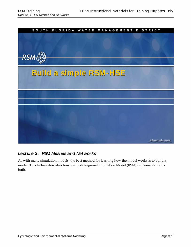
Session Objectives 1. To review how the Hydrologic Environmental Systems Modeling (HESM) team uses the XML schema for

organizing the RSM input and the advantages that the XML schema provides 2. To discuss content of the XML schema 3. To review the full XML input of typical RSM implementations by reviewing the content of several subregional

models

The subregional models show how we use the different functions available in the RSM to simulate the

hydrology and water management; water supply (WS) and flood control (FC) of south Florida.

Although the functions have been presented in the benchmarks and the HSE User Manual, actual

implementations of the functions are the best place to see and understand how the functions work,

what are typical ranges for the parameters, how the functions relate to other RSM components and

how the model performs i.e., output. In this module we review five different subregional

implementations. The key files of those subregional models are located in the $RSM/data directory in

your installation.

2

Session Objectives Session Objectives

Understand RSM XML Schema

• Input methods

• Input options

Understand RSM model construction

Create a simple RSM

Understand RSM XML Schema

• Input methods

• Input options

Understand RSM model construction

Create a simple RSM



3

Create a simple RSM Create a simple RSM

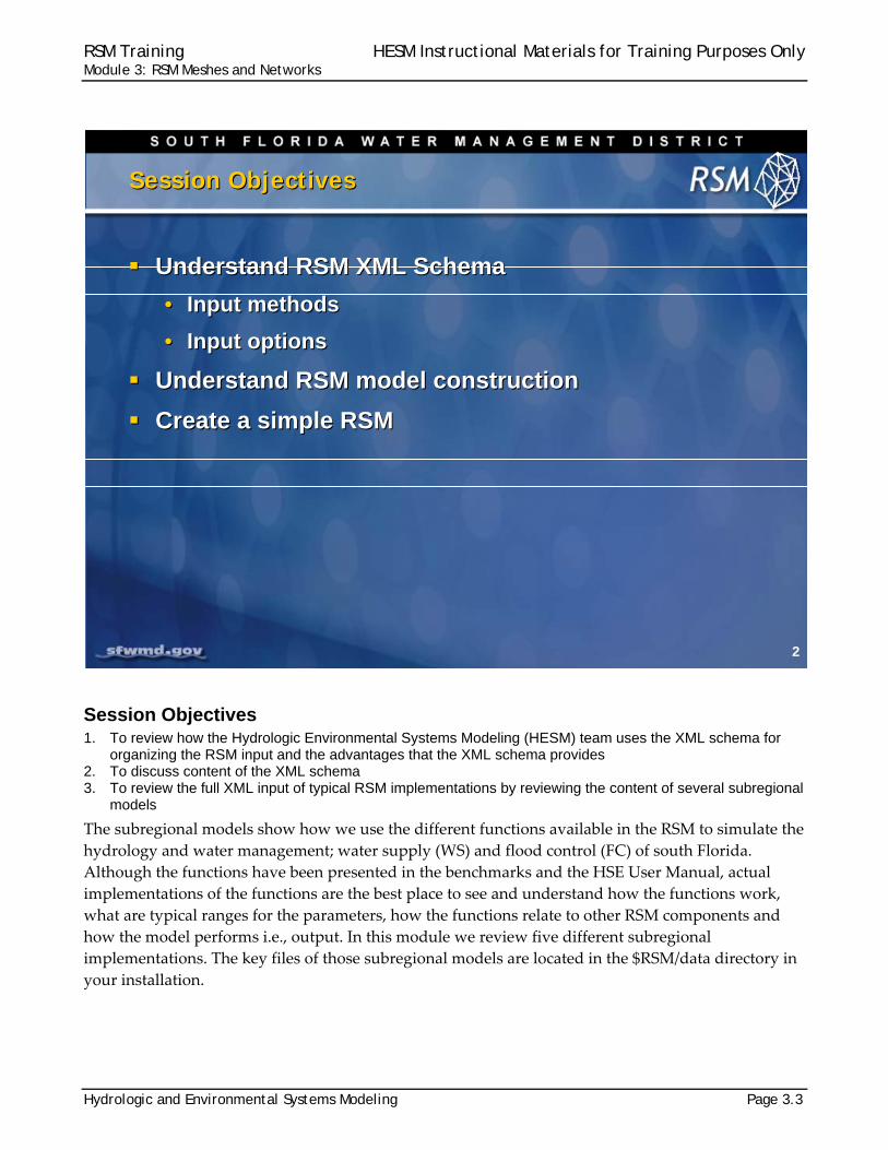
Input Data

Geographic data

Time series data

RSM components

Control

Mesh

Network

Outputs

Monitors

Budgets

Input Data

Geographic data

Time series data

RSM components

Control

Mesh

Network

Outputs

Monitors

Budgets



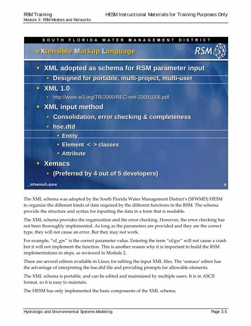
The XML schema was adopted by the South Florida Water Management District’s (SFWMD) HESM

to organize the different kinds of data required by the different functions in the RSM. The schema

provide the structure and syntax for inputting the data in a form that is readable.

The XML schema provides the organization and the error checking. However, the error checking has

not been thoroughly implemented. As long as the parameters are provided and they are the correct

type, they will not cause an error. But they may not work.

For example, “ol_gw” is the correct parameter value. Entering the term “ol/gw” will not cause a crash

but it will not implement the function. This is another reason why it is important to build the RSM

implementations in steps, as reviewed in Module 2.

There are several editors available in Linux for editing the input XML files. The ‘xemacs’ editor has

the advantage of interpreting the hse.dtd file and providing prompts for allowable elements.

The XML schema is portable, and can be edited and maintained by multiple users. It is in ASCII

format, so it is easy to maintain.

The HESM has only implemented the basic components of the XML schema.

4

eXtensible Markup LanguageeXtensible Markup Language

XML adopted as schema for RSM parameter input

• Designed for portable, multi-project, multi-user

XML 1.0• http://www.w3.org/TR/2000/REC-xml-20001006.pdf

XML input method

• Consolidation, error checking & completeness

• hse.dtd

Entity

Element < > classes

Attribute

Xemacs

• (Preferred by 4 out of 5 developers)




XML input method


• hse.dtd

Entity

Element < > classes

Attribute

Xemacs




(Continued)

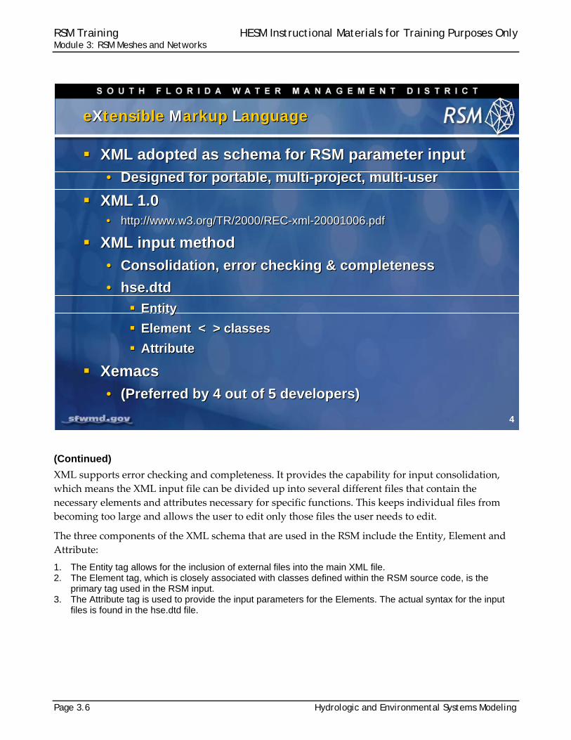
XML supports error checking and completeness. It provides the capability for input consolidation,

which means the XML input file can be divided up into several different files that contain the

necessary elements and attributes necessary for specific functions. This keeps individual files from

becoming too large and allows the user to edit only those files the user needs to edit.

The three components of the XML schema that are used in the RSM include the Entity, Element and

Attribute:

1. The Entity tag allows for the inclusion of external files into the main XML file. 2. The Element tag, which is closely associated with classes defined within the RSM source code, is the

primary tag used in the RSM input. 3. The Attribute tag is used to provide the input parameters for the Elements. The actual syntax for the input

files is found in the hse.dtd file.

4





XML input method


• hse.dtd

Entity

Element < > classes

Attribute

Xemacs





XML input method


• hse.dtd

Entity

Element < > classes

Attribute

Xemacs




(Continued)

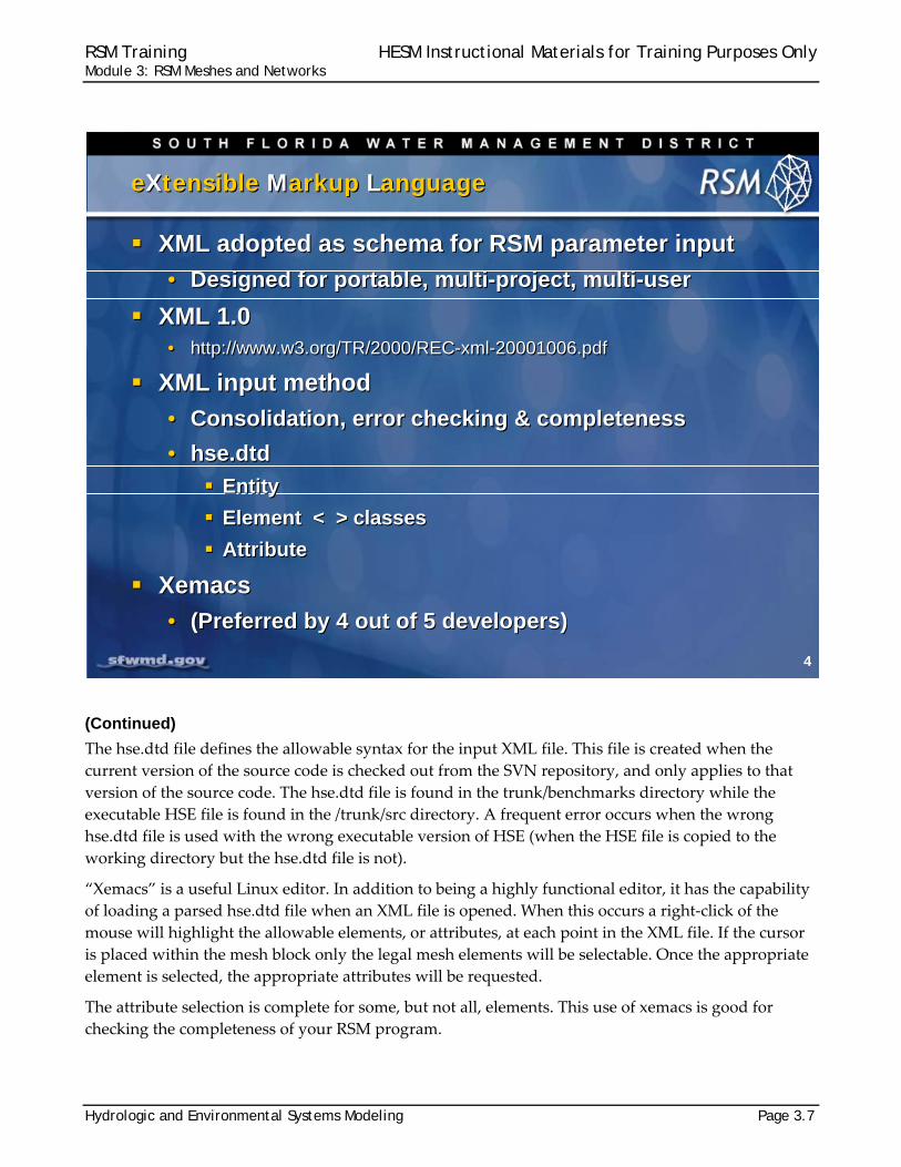
The hse.dtd file defines the allowable syntax for the input XML file. This file is created when the

current version of the source code is checked out from the SVN repository, and only applies to that

version of the source code. The hse.dtd file is found in the trunk/benchmarks directory while the

executable HSE file is found in the /trunk/src directory. A frequent error occurs when the wrong

hse.dtd file is used with the wrong executable version of HSE (when the HSE file is copied to the

working directory but the hse.dtd file is not).

“Xemacs” is a useful Linux editor. In addition to being a highly functional editor, it has the capability

of loading a parsed hse.dtd file when an XML file is opened. When this occurs a right‐click of the

mouse will highlight the allowable elements, or attributes, at each point in the XML file. If the cursor

is placed within the mesh block only the legal mesh elements will be selectable. Once the appropriate

element is selected, the appropriate attributes will be requested.

The attribute selection is complete for some, but not all, elements. This use of xemacs is good for

checking the completeness of your RSM program.

4





XML input method


• hse.dtd

Entity

Element < > classes

Attribute

Xemacs





XML input method


• hse.dtd

Entity

Element < > classes

Attribute

Xemacs




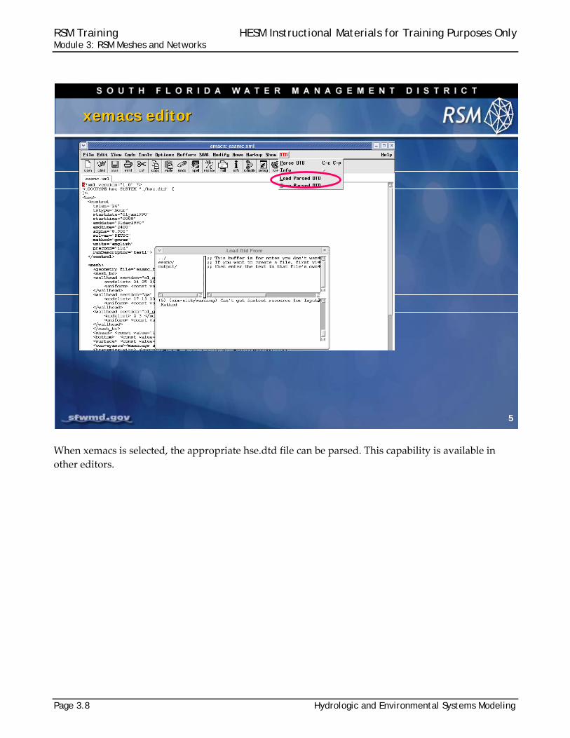
When xemacs is selected, the appropriate hse.dtd file can be parsed. This capability is available in

other editors.

5

xemacs editorxemacs editor



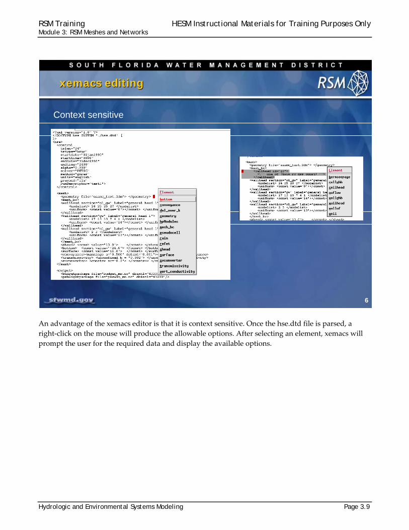
An advantage of the xemacs editor is that it is context sensitive. Once the hse.dtd file is parsed, a

right‐click on the mouse will produce the allowable options. After selecting an element, xemacs will

prompt the user for the required data and display the available options.

6

xemacs editingxemacs editing

Context sensitive



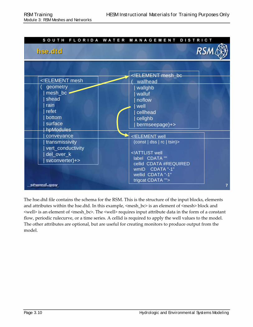
The hse.dtd file contains the schema for the RSM. This is the structure of the input blocks, elements

and attributes within the hse.dtd. In this example, <mesh_bc> is an element of <mesh> block and

<well> is an element of <mesh_bc>. The <well> requires input attribute data in the form of a constant

flow, periodic rulecurve, or a time series. A cellid is required to apply the well values to the model.

The other attributes are optional, but are useful for creating monitors to produce output from the

model.

7

hse.dtdhse.dtd

<!ELEMENT mesh( geometry

| mesh_bc| shead| rain| refet| bottom| surface| hpModules| conveyance| transmissivity| vert_conductivity| del_over_k| svconverter)+>

<!ELEMENT mesh_bc( wallhead| wallghb| walluf| noflow| well| cellhead| cellghb| bermseepage)+>

<!ELEMENT well(const | dss | rc | tsin)>

<!ATTLIST welllabel CDATA ""cellid CDATA #REQUIREDwmID CDATA "-1"wellid CDATA "-1"trigcat CDATA "">



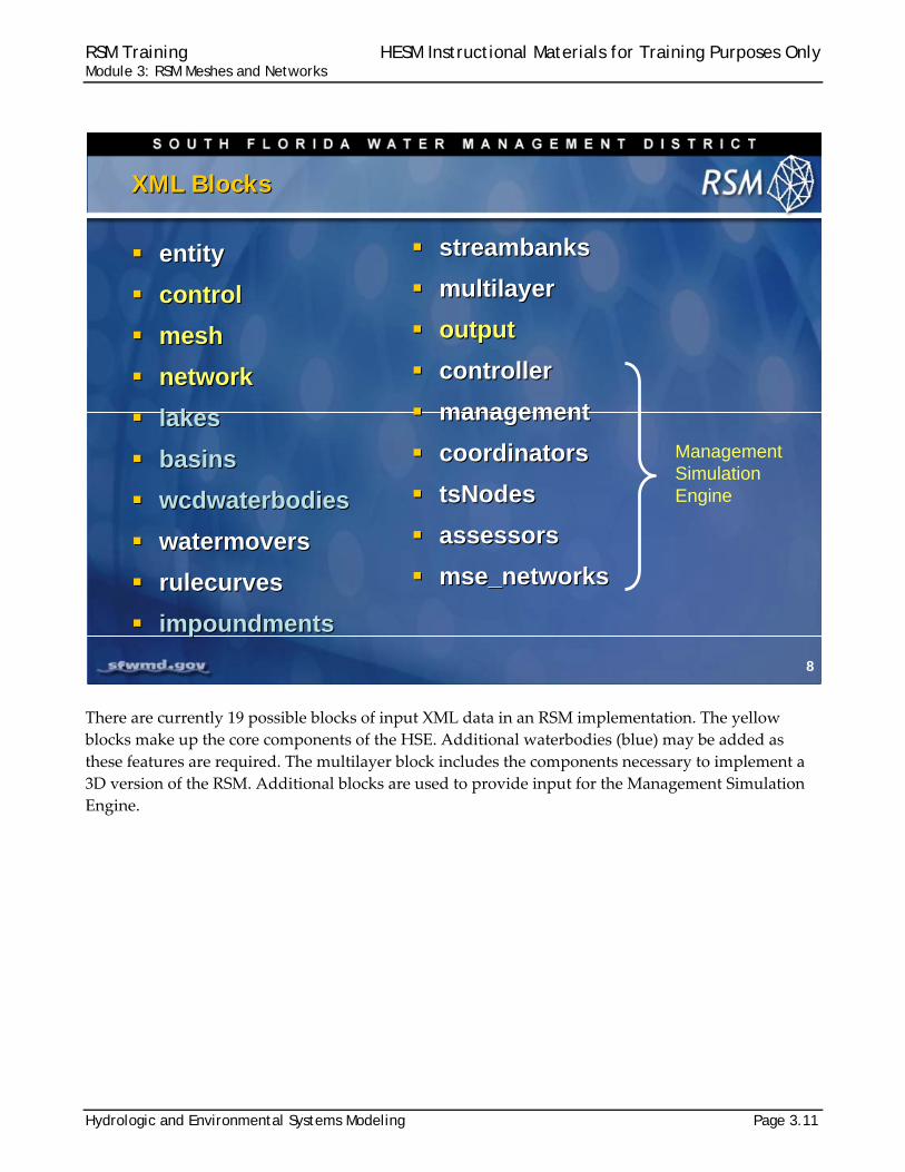
There are currently 19 possible blocks of input XML data in an RSM implementation. The yellow

blocks make up the core components of the HSE. Additional waterbodies (blue) may be added as

these features are required. The multilayer block includes the components necessary to implement a

3D version of the RSM. Additional blocks are used to provide input for the Management Simulation

Engine.

8

XML BlocksXML Blocks

entity

control

mesh

network

lakes

basins

wcdwaterbodies

watermovers

rulecurves

impoundments

entity

control

mesh

network

lakes

basins

wcdwaterbodies

watermovers

rulecurves

impoundments

streambanks

multilayer

output

controller

management

coordinators

tsNodes

assessors

mse_networks

streambanks

multilayer

output

controller

management

coordinators

tsNodes

assessors

mse_networks

Management Simulation Engine



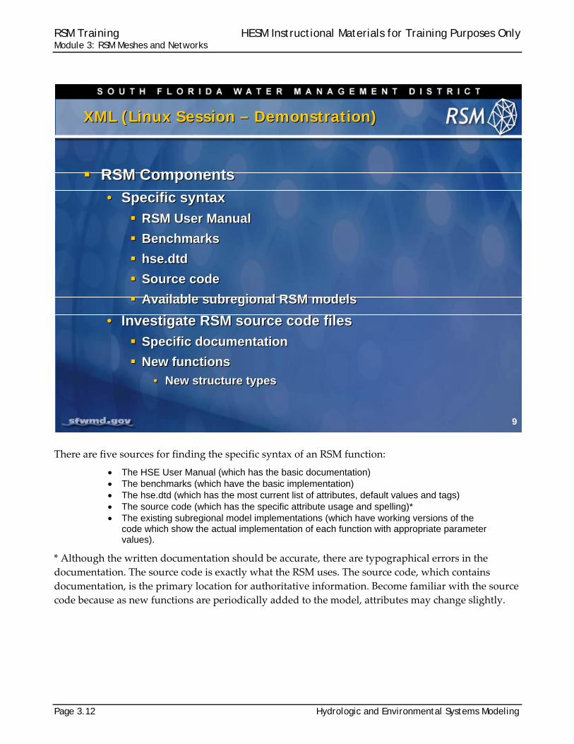
There are five sources for finding the specific syntax of an RSM function:

The HSE User Manual (which has the basic documentation) The benchmarks (which have the basic implementation) The hse.dtd (which has the most current list of attributes, default values and tags) The source code (which has the specific attribute usage and spelling)* The existing subregional model implementations (which have working versions of the

code which show the actual implementation of each function with appropriate parameter values).

* Although the written documentation should be accurate, there are typographical errors in the

documentation. The source code is exactly what the RSM uses. The source code, which contains

documentation, is the primary location for authoritative information. Become familiar with the source

code because as new functions are periodically added to the model, attributes may change slightly.

9

XML (Linux Session – Demonstration)XML (Linux Session – Demonstration)

RSM Components

• Specific syntax

RSM User Manual

Benchmarks

hse.dtd

Source code

Available subregional RSM models

• Investigate RSM source code files

Specific documentation

New functions

• New structure types

RSM Components

• Specific syntax

RSM User Manual

Benchmarks

hse.dtd

Source code

Available subregional RSM models

• Investigate RSM source code files

Specific documentation

New functions

• New structure types



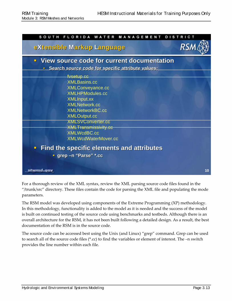
For a thorough review of the XML syntax, review the XML parsing source code files found in the

“/trunk/src” directory. These files contain the code for parsing the XML file and populating the mode

parameters.

The RSM model was developed using components of the Extreme Programming (XP) methodology.

In this methodology, functionality is added to the model as it is needed and the success of the model

is built on continued testing of the source code using benchmarks and testbeds. Although there is an

overall architecture for the RSM, it has not been built following a detailed design. As a result, the best

documentation of the RSM is in the source code.

The source code can be accessed best using the Unix (and Linux) “grep” command. Grep can be used

to search all of the source code files (*.cc) to find the variables or element of interest. The –n switch

provides the line number within each file.

10


View source code for current documentation• Search source code for specific attribute values:

Find the specific elements and attributes grep –n “Parse” *.cc

View source code for current documentation• Search source code for specific attribute values:

Find the specific elements and attributes grep –n “Parse” *.cc

fvsetup.ccXMLBasins.ccXMLConveyance.ccXMLHPModules.ccXMLInput.xxXMLNetwork.ccXMLNetworkBC.ccXMLOutput.ccXMLSVConverter.ccXMLTransmissivity.ccXMLWcdBC.ccXMLWcdWaterMover.cc



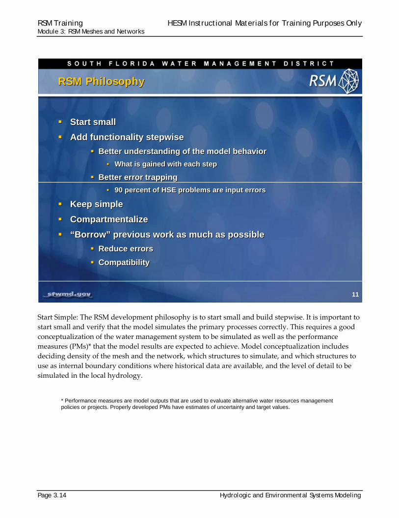
Start Simple: The RSM development philosophy is to start small and build stepwise. It is important to

start small and verify that the model simulates the primary processes correctly. This requires a good

conceptualization of the water management system to be simulated as well as the performance

measures (PMs)* that the model results are expected to achieve. Model conceptualization includes

deciding density of the mesh and the network, which structures to simulate, and which structures to

use as internal boundary conditions where historical data are available, and the level of detail to be

simulated in the local hydrology.

* Performance measures are model outputs that are used to evaluate alternative water resources management policies or projects. Properly developed PMs have estimates of uncertainty and target values.

11

RSM PhilosophyRSM Philosophy

Start small

Add functionality stepwise

Better understanding of the model behavior

• What is gained with each step

Better error trapping

• 90 percent of HSE problems are input errors

Keep simple

Compartmentalize

“Borrow” previous work as much as possible

Reduce errors

Compatibility

Start small






Keep simple

Compartmentalize


Reduce errors

Compatibility



(Continued)

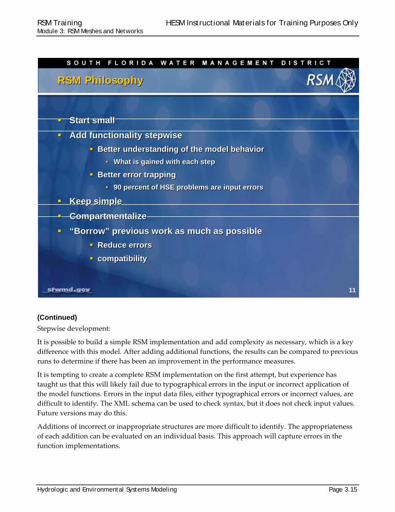
Stepwise development:

It is possible to build a simple RSM implementation and add complexity as necessary, which is a key

difference with this model. After adding additional functions, the results can be compared to previous

runs to determine if there has been an improvement in the performance measures.

It is tempting to create a complete RSM implementation on the first attempt, but experience has

taught us that this will likely fail due to typographical errors in the input or incorrect application of

the model functions. Errors in the input data files, either typographical errors or incorrect values, are

difficult to identify. The XML schema can be used to check syntax, but it does not check input values.

Future versions may do this.

Additions of incorrect or inappropriate structures are more difficult to identify. The appropriateness

of each addition can be evaluated on an individual basis. This approach will capture errors in the

function implementations.

11

RSM PhilosophyRSM Philosophy

Start small






Keep simple

Compartmentalize


Reduce errors

compatibility

Start small






Keep simple

Compartmentalize


Reduce errors

compatibility



Manually building a simple RSM application is one of the best ways to learn the model components,

as well as how to run the RSM and how to view the typical results.

Lecture 3A: Build RSM-HSE by handLecture 3A: Build RSM-HSE by hand



A simple RSM application will include these blocks and the appropriate input data. The sample.xml

file provided in the labs/lab3_simple_RSM directory contains the detailed elements of each

block. Each block is discussed on the following pages.

13

Simple RSM-HSE: sample.xmlSimple RSM-HSE: sample.xml

Control blocks

• Model run parameters

Mesh

• Cell geometry

• Boundary conditions

Network

• Canal geometry

• Segment properties

Output

• Monitors

• Budget packages(see handout: sample.xml)

Control blocks

• Model run parameters

Mesh

• Cell geometry


Network

• Canal geometry

• Segment properties

Output

• Monitors

• Budget packages(see handout: sample.xml)



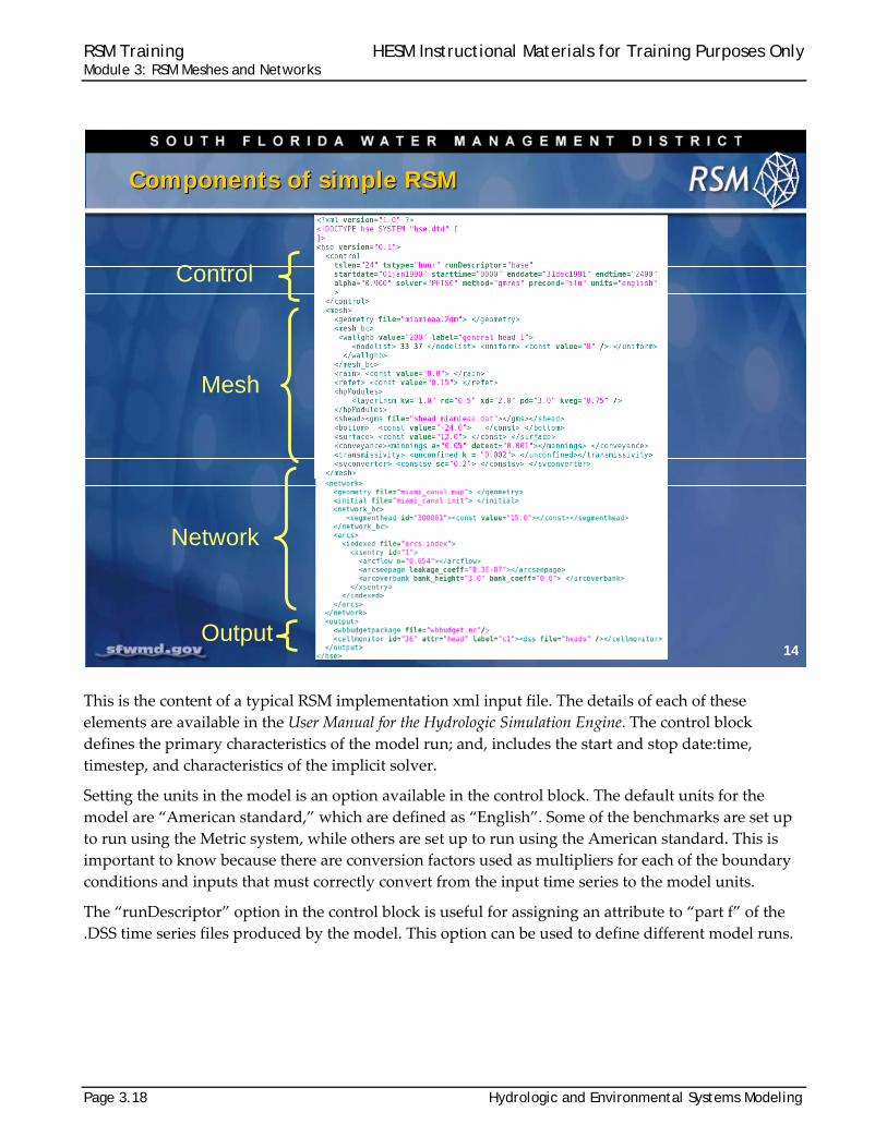
This is the content of a typical RSM implementation xml input file. The details of each of these

elements are available in the User Manual for the Hydrologic Simulation Engine. The control block

defines the primary characteristics of the model run; and, includes the start and stop date:time,

timestep, and characteristics of the implicit solver.

Setting the units in the model is an option available in the control block. The default units for the

model are “American standard,” which are defined as “English”. Some of the benchmarks are set up

to run using the Metric system, while others are set up to run using the American standard. This is

important to know because there are conversion factors used as multipliers for each of the boundary

conditions and inputs that must correctly convert from the input time series to the model units.

The “runDescriptor” option in the control block is useful for assigning an attribute to “part f” of the

.DSS time series files produced by the model. This option can be used to define different model runs.

14

Components of simple RSM Components of simple RSM

Control

Network

Mesh

Output



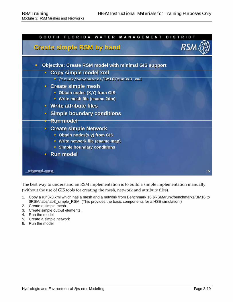
The best way to understand an RSM implementation is to build a simple implementation manually

(without the use of GIS tools for creating the mesh, network and attribute files).

1. Copy a run3x3.xml which has a mesh and a network from Benchmark 16 $RSM/trunk/benchmarks/BM16 to $RSM/labs/lab3_simple_RSM. (This provides the basic components for a HSE simulation.)

2. Create a simple mesh. 3. Create simple output elements. 4. Run the model 5. Create a simple network 6. Run the model

15

Create simple RSM by handCreate simple RSM by hand

Objective: Create RSM model with minimal GIS support

• Copy simple model xml /trunk/benchmarks/BM16/run3x3.xml

• Create simple mesh Obtain nodes (X,Y) from GIS

Write mesh file (eaamc.2dm)

• Write attribute files

• Simple boundary conditions

• Run model

• Create simple Network Obtain nodes(x,y) from GIS

Write network file (eaamc.map)

Simple boundary conditions

• Run model

Objective: Create RSM model with minimal GIS support

• Copy simple model xml /trunk/benchmarks/BM16/run3x3.xml

• Create simple mesh Obtain nodes (X,Y) from GIS

Write mesh file (eaamc.2dm)

• Write attribute files

• Simple boundary conditions

• Run model

• Create simple Network Obtain nodes(x,y) from GIS

Write network file (eaamc.map)

Simple boundary conditions

• Run model



The EAA‐Miami Canal Basin was selected for this exercise. It consists of three subbasins; the S3‐S8,

the Rotenberger and the Holey Land. There is one major canal, the Miami Canal, and several smaller

canals. The primary landuse is sugar cane agriculture in the S3‐S8 and native scrub and marsh in the

Rotenberger and Holey Land.

16

EAA-Miami Canal BasinEAA-Miami Canal Basin



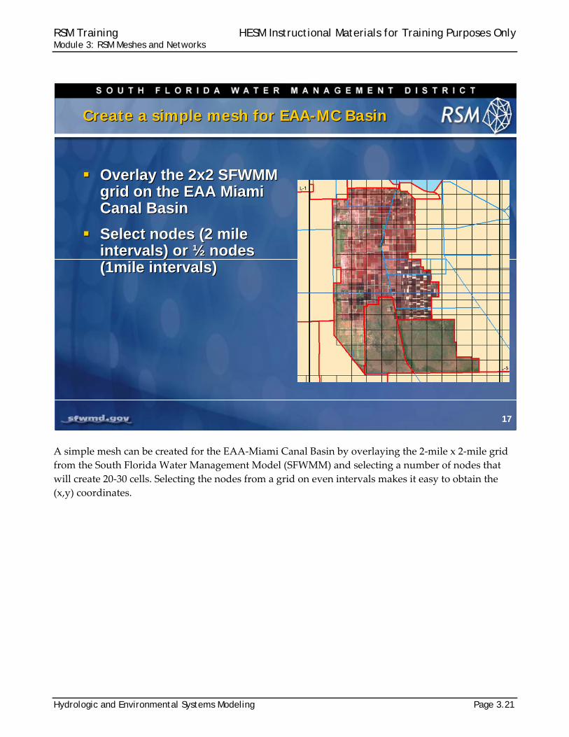
A simple mesh can be created for the EAA‐Miami Canal Basin by overlaying the 2‐mile x 2‐mile grid

from the South Florida Water Management Model (SFWMM) and selecting a number of nodes that

will create 20‐30 cells. Selecting the nodes from a grid on even intervals makes it easy to obtain the

(x,y) coordinates.

17

Create a simple mesh for EAA-MC BasinCreate a simple mesh for EAA-MC Basin

Overlay the 2x2 SFWMM grid on the EAA Miami Canal Basin

Select nodes (2 mile intervals) or ½ nodes (1mile intervals)

Overlay the 2x2 SFWMM grid on the EAA Miami Canal Basin

Select nodes (2 mile intervals) or ½ nodes (1mile intervals)



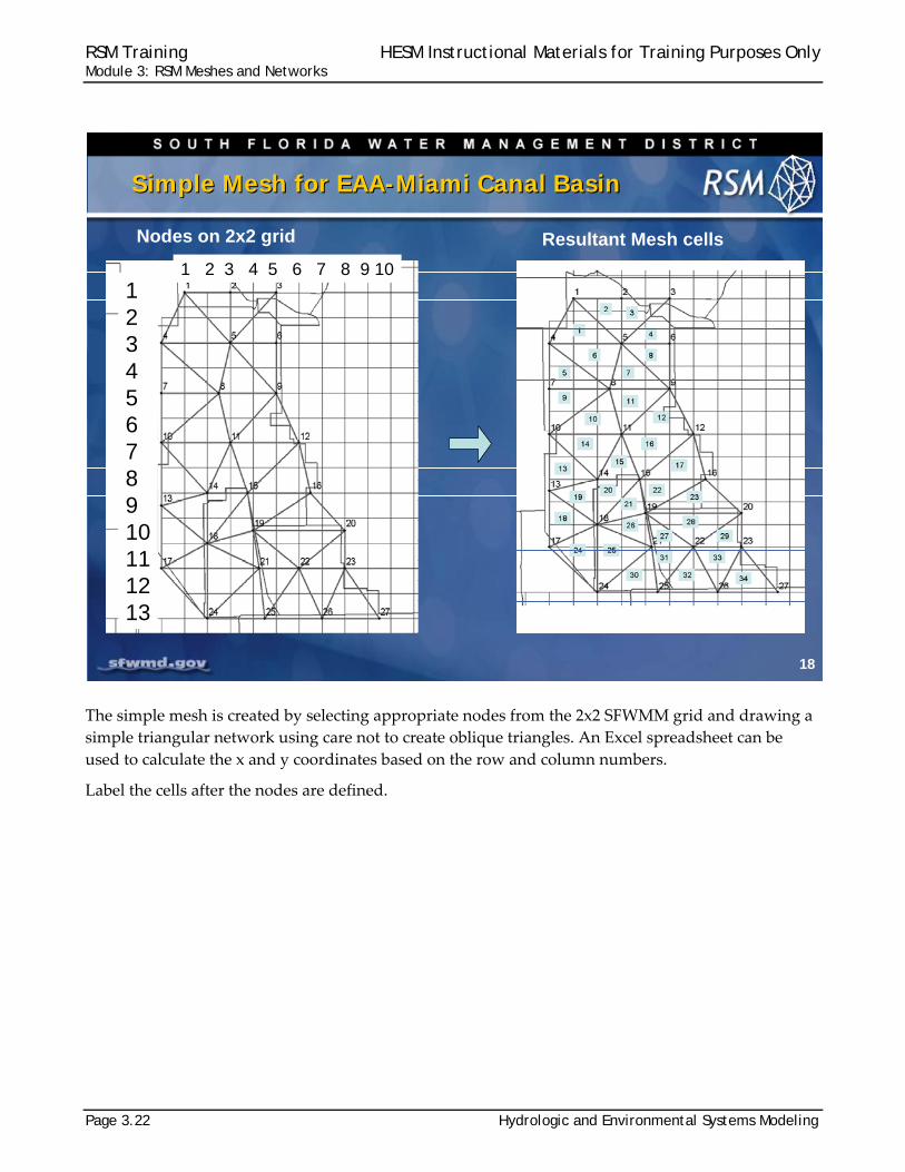
The simple mesh is created by selecting appropriate nodes from the 2x2 SFWMM grid and drawing a

simple triangular network using care not to create oblique triangles. An Excel spreadsheet can be

used to calculate the x and y coordinates based on the row and column numbers.

Label the cells after the nodes are defined.

18

Simple Mesh for EAA-Miami Canal BasinSimple Mesh for EAA-Miami Canal Basin

Nodes on 2x2 grid Resultant Mesh cells

12345678910111213

1 2 3 4 5 6 7 8 9 10



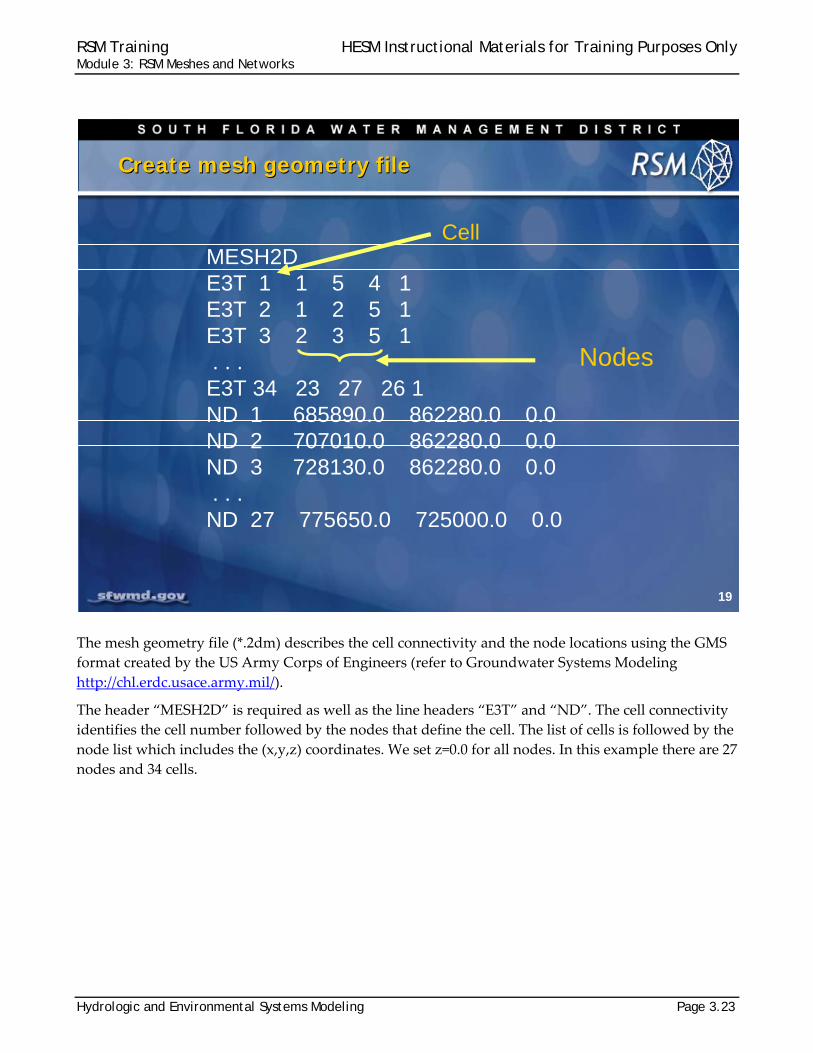
The mesh geometry file (*.2dm) describes the cell connectivity and the node locations using the GMS

format created by the US Army Corps of Engineers (refer to Groundwater Systems Modeling

http://chl.erdc.usace.army.mil/).

The header “MESH2D” is required as well as the line headers “E3T” and “ND”. The cell connectivity

identifies the cell number followed by the nodes that define the cell. The list of cells is followed by the

node list which includes the (x,y,z) coordinates. We set z=0.0 for all nodes. In this example there are 27

nodes and 34 cells.

19

Create mesh geometry fileCreate mesh geometry file

MESH2DE3T 1 1 5 4 1E3T 2 1 2 5 1E3T 3 2 3 5 1. . .

E3T 34 23 27 26 1ND 1 685890.0 862280.0 0.0ND 2 707010.0 862280.0 0.0ND 3 728130.0 862280.0 0.0. . .

ND 27 775650.0 725000.0 0.0

Cell

Nodes



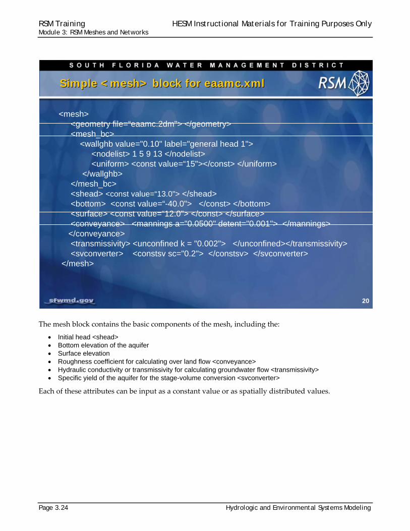
The mesh block contains the basic components of the mesh, including the:

Initial head <shead> Bottom elevation of the aquifer Surface elevation Roughness coefficient for calculating over land flow <conveyance> Hydraulic conductivity or transmissivity for calculating groundwater flow <transmissivity> Specific yield of the aquifer for the stage-volume conversion <svconverter>

Each of these attributes can be input as a constant value or as spatially distributed values.

20

Simple <mesh> block for eaamc.xmlSimple <mesh> block for eaamc.xml

<mesh><geometry file=“eaamc.2dm"> </geometry> <mesh_bc>

<wallghb value="0.10" label="general head 1"> <nodelist> 1 5 9 13 </nodelist> <uniform> <const value=“15"></const> </uniform>

</wallghb></mesh_bc><shead> <const value=“13.0"> </shead><bottom> <const value=“-40.0"> </const> </bottom><surface> <const value=“12.0"> </const> </surface><conveyance> <mannings a="0.0500" detent="0.001"> </mannings> </conveyance> <transmissivity> <unconfined k = "0.002"> </unconfined></transmissivity><svconverter> <constsv sc="0.2"> </constsv> </svconverter>

</mesh>



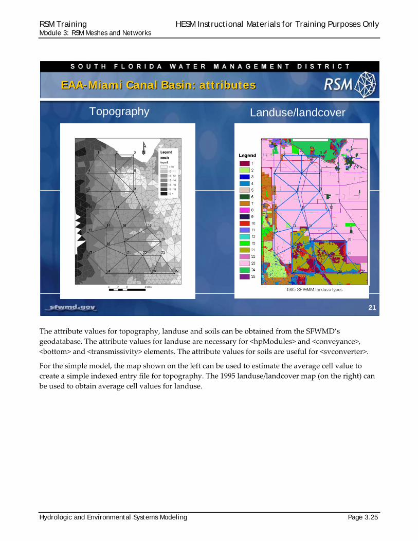
The attribute values for topography, landuse and soils can be obtained from the SFWMD’s

geodatabase. The attribute values for landuse are necessary for <hpModules> and <conveyance>,

<bottom> and <transmissivity> elements. The attribute values for soils are useful for <svconverter>.

For the simple model, the map shown on the left can be used to estimate the average cell value to

create a simple indexed entry file for topography. The 1995 landuse/landcover map (on the right) can

be used to obtain average cell values for landuse.

21

EAA-Miami Canal Basin: attributesEAA-Miami Canal Basin: attributes

Topography Landuse/landcover



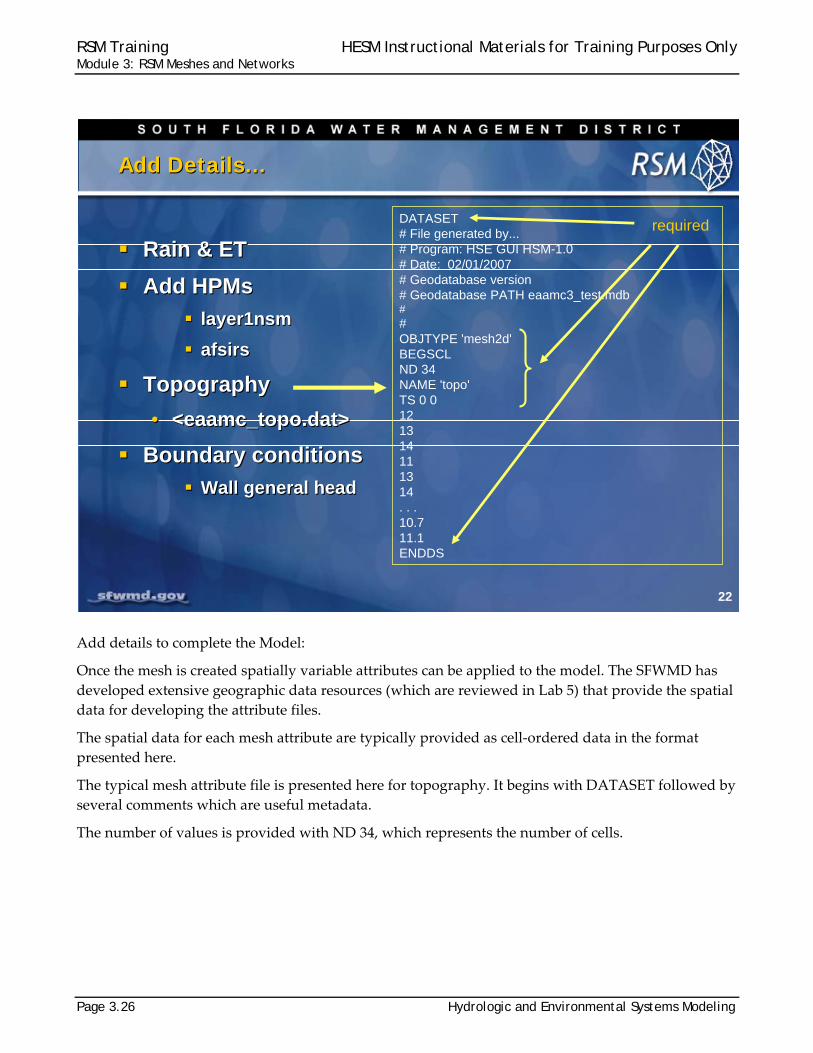
Add details to complete the Model:

Once the mesh is created spatially variable attributes can be applied to the model. The SFWMD has

developed extensive geographic data resources (which are reviewed in Lab 5) that provide the spatial

data for developing the attribute files.

The spatial data for each mesh attribute are typically provided as cell‐ordered data in the format

presented here.

The typical mesh attribute file is presented here for topography. It begins with DATASET followed by

several comments which are useful metadata.

The number of values is provided with ND 34, which represents the number of cells.

22

Add Details…Add Details…

Rain & ET

Add HPMs

layer1nsm

afsirs

Topography

• <eaamc_topo.dat>

Boundary conditions

Wall general head

Rain & ET

Add HPMs

layer1nsm

afsirs

Topography

• <eaamc_topo.dat>

Boundary conditions

Wall general head

DATASET# File generated by...# Program: HSE GUI HSM-1.0# Date: 02/01/2007# Geodatabase version# Geodatabase PATH eaamc3_test.mdb##OBJTYPE 'mesh2d'BEGSCLND 34NAME 'topo'TS 0 0121314111314. . .10.711.1ENDDS

required



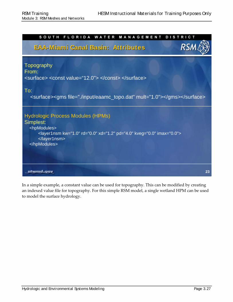
In a simple example, a constant value can be used for topography. This can be modified by creating

an indexed value file for topography. For this simple RSM model, a single wetland HPM can be used

to model the surface hydrology.

23

TopographyFrom:<surface> <const value=“12.0"> </const> </surface>

To:<surface><gms file="./input/eaamc_topo.dat" mult="1.0"></gms></surface>

Hydrologic Process Modules (HPMs)Simplest:

<hpModules><layer1nsm kw="1.0" rd="0.0" xd="1.2" pd="4.0" kveg="0.0" imax="0.0"> </layer1nsm>

</hpModules>

EAA-Miami Canal Basin: AttributesEAA-Miami Canal Basin: Attributes



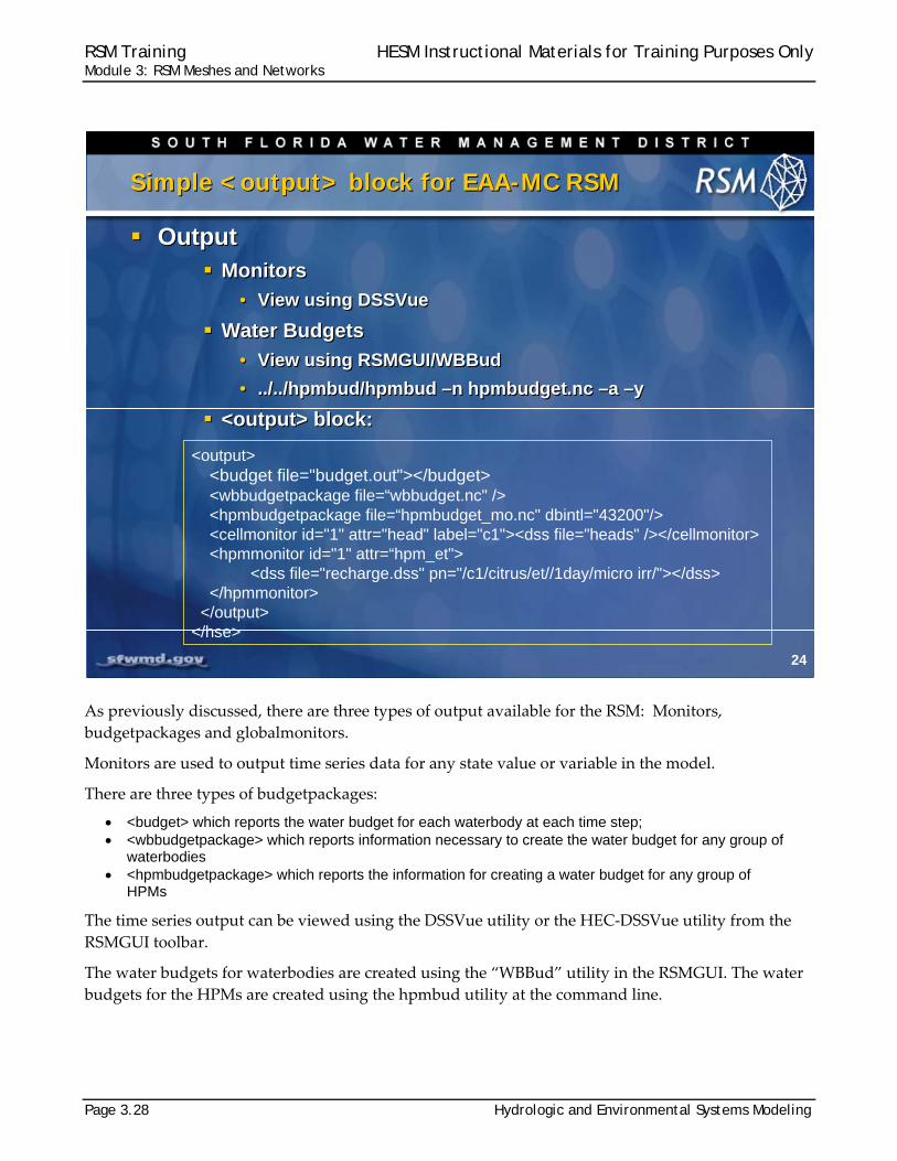
As previously discussed, there are three types of output available for the RSM: Monitors,

budgetpackages and globalmonitors.

Monitors are used to output time series data for any state value or variable in the model.

There are three types of budgetpackages:

<budget> which reports the water budget for each waterbody at each time step; <wbbudgetpackage> which reports information necessary to create the water budget for any group of

waterbodies <hpmbudgetpackage> which reports the information for creating a water budget for any group of

HPMs

The time series output can be viewed using the DSSVue utility or the HEC‐DSSVue utility from the

RSMGUI toolbar.

The water budgets for waterbodies are created using the “WBBud” utility in the RSMGUI. The water

budgets for the HPMs are created using the hpmbud utility at the command line.

24

Simple <output> block for EAA-MC RSMSimple <output> block for EAA-MC RSM

Output Monitors

• View using DSSVue

Water Budgets

• View using RSMGUI/WBBud

• ../../hpmbud/hpmbud –n hpmbudget.nc –a –y

<output> block:

Output Monitors

• View using DSSVue

Water Budgets

• View using RSMGUI/WBBud

• ../../hpmbud/hpmbud –n hpmbudget.nc –a –y

<output> block:

<output><budget file="budget.out"></budget><wbbudgetpackage file=“wbbudget.nc" /><hpmbudgetpackage file=“hpmbudget_mo.nc" dbintl="43200"/><cellmonitor id="1" attr="head" label="c1"><dss file="heads" /></cellmonitor><hpmmonitor id="1" attr=“hpm_et">

<dss file="recharge.dss" pn="/c1/citrus/et//1day/micro irr/"></dss></hpmmonitor>

</output></hse>



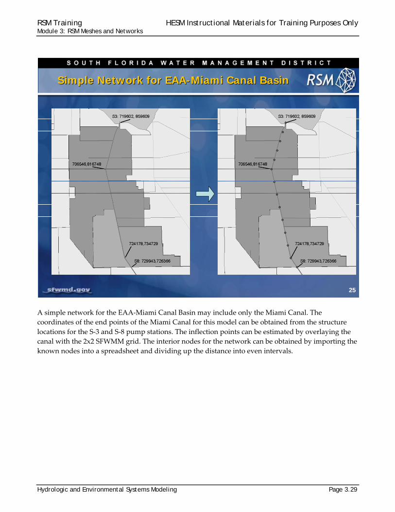
A simple network for the EAA‐Miami Canal Basin may include only the Miami Canal. The

coordinates of the end points of the Miami Canal for this model can be obtained from the structure

locations for the S‐3 and S‐8 pump stations. The inflection points can be estimated by overlaying the

canal with the 2x2 SFWMM grid. The interior nodes for the network can be obtained by importing the

known nodes into a spreadsheet and dividing up the distance into even intervals.

25

Simple Network for EAA-Miami Canal BasinSimple Network for EAA-Miami Canal Basin



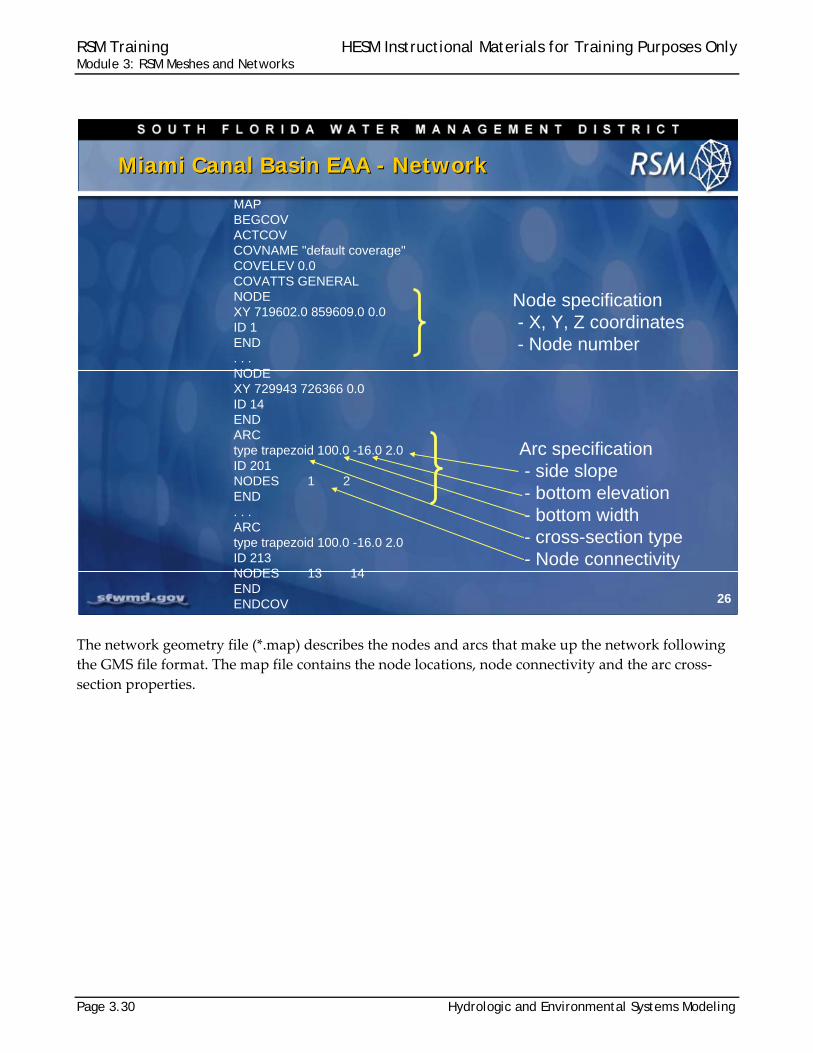
The network geometry file (*.map) describes the nodes and arcs that make up the network following

the GMS file format. The map file contains the node locations, node connectivity and the arc cross‐

section properties.

26

Miami Canal Basin EAA - NetworkMiami Canal Basin EAA - Network

MAPBEGCOVACTCOVCOVNAME "default coverage"COVELEV 0.0COVATTS GENERALNODEXY 719602.0 859609.0 0.0ID 1END. . .NODEXY 729943 726366 0.0ID 14ENDARCtype trapezoid 100.0 -16.0 2.0ID 201NODES 1 2END. . .ARCtype trapezoid 100.0 -16.0 2.0ID 213NODES 13 14ENDENDCOV

Node specification- X, Y, Z coordinates- Node number

Arc specification- side slope- bottom elevation- bottom width- cross-section type- Node connectivity



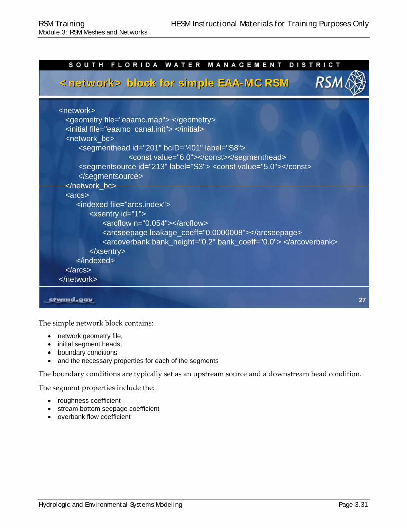
The simple network block contains:

network geometry file, initial segment heads, boundary conditions and the necessary properties for each of the segments

The boundary conditions are typically set as an upstream source and a downstream head condition.

The segment properties include the:

roughness coefficient stream bottom seepage coefficient overbank flow coefficient

27

<network> block for simple EAA-MC RSM<network> block for simple EAA-MC RSM

<network><geometry file="eaamc.map"> </geometry><initial file="eaamc_canal.init"> </initial><network_bc>

<segmenthead id="201" bcID="401" label="S8"><const value="6.0"></const></segmenthead>

<segmentsource id="213" label="S3"> <const value="5.0"></const> </segmentsource>

</network_bc> <arcs>

<indexed file="arcs.index"><xsentry id="1">

<arcflow n="0.054"></arcflow><arcseepage leakage_coeff="0.0000008"></arcseepage><arcoverbank bank_height="0.2" bank_coeff="0.0"> </arcoverbank>

</xsentry></indexed>

</arcs></network>



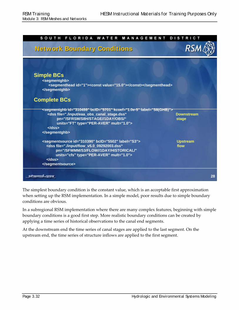
The simplest boundary condition is the constant value, which is an acceptable first approximation

when setting up the RSM implementation. In a simple model, poor results due to simple boundary

conditions are obvious.

In a subregional RSM implementation where there are many complex features, beginning with simple

boundary conditions is a good first step. More realistic boundary conditions can be created by

applying a time series of historical observations to the canal end segments.

At the downstream end the time series of canal stages are applied to the last segment. On the

upstream end, the time series of structure inflows are applied to the first segment.

28

Network Boundary ConditionsNetwork Boundary Conditions

Simple BCs<segmentghb>

<segmenthead id="1"><const value="15.0"></const></segmenthead></segmentghb>

Complete BCs

<segmentghb id="310459" bcID="5701" kcoef="1.0e-5" label="S8(GHB)"><dss file="./input/eaa_obs_canal_stage.dss“ Downstream

pn="/SFRSM/S8H/STAGE//1DAY/OBS/“ stageunits="FT" type="PER-AVER" mult="1.0">

</dss></segmentghb>

<segmentsource id="310390" bcID="5502" label="S3"> Upstream<dss file="./input/flow_v5.0_09292003.dss“ flow

pn="/SFWMM/S3/FLOW//1DAY/HISTORICAL/"units="cfs" type="PER-AVER" mult="1.0">

</dss></segmentsource>



In this lecture we reviewed the steps for creating an RSM implementation without the benefit of GIS.

This session highlights the construction and content of the key files used to create an RSM input

dataset.

29

SummarySummary

Mesh files

• sample.2dm

• Indexed hpms

• Rainfall & PET files• District rainfall and pet *.bin files

• Indexed topography


Network files

• Sample.map

• Boundary conditions WMM *.dss files

Output files

• Water budgets

• monitors

Mesh files

• sample.2dm

• Indexed hpms

• Rainfall & PET files• District rainfall and pet *.bin files

• Indexed topography


Network files

• Sample.map

• Boundary conditions WMM *.dss files

Output files

• Water budgets

• monitors





Knowledge Assessment

1. What is the purpose for using XMLs? 2. What is the advantage of using the Xemacs or similar editor? 3. What are the essential components of XML used in RSM? 4. What are the key XML blocks used in RSM? 5. What are the best sources of syntax for implementing features in RSM? 6. How does indexed input work? 7. What are the key principles to follow in development of a new RSM implementation? 8. What are the components of a 2dm file? 9. What are the necessary elements of a mesh block? 10. What are the common three ways to represent topography? 11. Two common types of RSM output? 12. What are the components of a .map file?



Answers 1. The Extensible Markup Language is used to provide a portable, complete input

schema that provides error checking capability. 2. Xemacs and similar editors are context sensitive and can be used with the hse.dtd file

to provide only the input elements and attributes that are appropriate for each input block.

3. The RSM uses blocks, elements and attributes to define the model input parameters. 4. The key XML blocks are the following: Control, Mesh, Network and Output. 5. The syntax for RSM can be found in the HSE User Manual and for new features:

benchmarks, hse.dtd and the source code. The input files from current RSM implementations can be borrowed to avoid typing errors.

6. The index input file follows the GMS format for header information followed by an

ordered list of attribute values for each cell or segment. There are no segment or cell identifiers.

7. It is important to start small and add features stepwise. Only add complexity as

necessary. Compartmentalize the XML input and the model features. Borrow input syntax such as HPMs, boundary conditions and network features from previous implementations.

8. The 2dm file contains the mesh_node connectivity and mesh_node locations. 9. <geometry>, <shead>, <surface>, <bottom>, <conveyance> and <transmissivity> 10. Topography can be entered as a constant, an indexed file or a gms file. 11. The two types of output are “monitors” and budget data in netCDF files. 12. The map file contains: node connectivity, cross-section properties, segment

connectivity.



Lab 3: Frameworks, Meshes and Networks

Time Estimate: 1.5 hours

Training Objective: Build a simple mesh and network

To understand how the Regional Simulation Model (RSM) behaves it is appropriate to

build a simple RSM manually. This will provide the user with a basic understanding of

the information used by the RSM to create the objects that run the model.

Although a simple RSM model can be built manually, a subregional model requires

Geographic Information System (GIS) tools to construct the necessary input files of

spatially distributed data. There are automated tools used to create the necessary input

files, which will be presented in Labs 6 and 7.

The first two spatial input files created for the RSM are a mesh file and the network

file. In this lab, you will create a small mesh file and a small network file, and run a

simple RSM implementation.

Build a simple RSM-HSEBuild a simple RSM-HSE



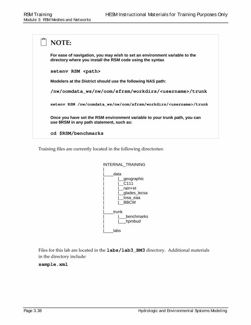
NOTE:

For ease of navigation, you may wish to set an environment variable to the directory where you install the RSM code using the syntax

setenv RSM <path>

Modelers at the District should use the following NAS path:

/nw/oomdata_ws/nw/oom/sfrsm/workdirs/<username>/trunk

setenv RSM /nw/oomdata_ws/nw/oom/sfrsm/workdirs/<username>/trunk

Once you have set the RSM environment variable to your trunk path, you can use $RSM in any path statement, such as:

cd $RSM/benchmarks

Training files are currently located in the following directories:

INTERNAL_TRAINING | |____data | |__geographic | |__C111 | |__rain+et | |__glades_lecsa | |__losa_eaa | |__BBCW | |____trunk | |___benchmarks | |___hpmbud | |____labs

Files for this lab are located in the labs/lab3_BM3 directory. Additional materials

in the directory include:

sample.xml



Activity 3.1: Manually create a simple mesh and network for the EAA-MC Basin RSM

Overview

Activity 3.1 includes two exercises:

Exercise 3.1.1 Create a mesh for the EAA-MC Basin Exercise 3.1.2 Create a network for the EAA-MC Basin

You will manually create a mesh and network for the Everglades Agricultural Area‐

Miami Canal (EAA‐MC) Basin (see Fig 3.1)

Exercise 3.1.1 Create a simple mesh for the EAA-MC Basin

First, examine the content of a simple benchmark mesh file (Fig. 3.2). The mesh.2dm is

an ASCII file that contains two sections:

1. The cell connectivity section that has a row for each cell containing the cell id and the three

nodes that form each cell in clockwise order

2. The node coordinate location section that has a row for each node containing the node id

and the x-y-z coordinates for that node including a

zero-coordinate value for the z-axis.

The cell connectivity section of the mesh.2dm file contains an additional parameter

which is not used, but set to 1.0. The format for the mesh.2dm is a standard mesh

format from the Groundwater Modeling System (GMS) package (which is discussed in

Lab 6).

To create any mesh in south Florida, start with the simple two‐mile by two‐mile grid

used for the South Florida Water Management Model (SFWMM) (Fig. 3.3). The 2x2

grid is useful because we have a substantial amount of hydrologic information from

the SFWMM associated with this grid.

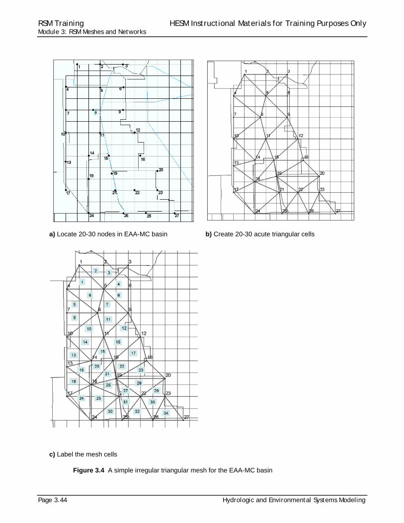
For the EAA‐MC Basin select a set of nodes that will result in 20–30 triangular cells that

are approximately the same size and acute, with no angle greater than 90 degrees. Use

the portion of the grid that includes the EAA‐MC (Fig.3.3).

The lowest y-coordinate of the EAA‐MC grid is 725000 and the lowest x-coordinate is

675330. Make the mesh conform to the Rotenberger Subbasin and the Holeyland

Subbasin.

3. Using the intersects of the SFWMM grid in Fig 3.3, create nodes for the RSM triangular

mesh.(Your resulting nodes should be distributed in a manner similar to the nodes as they

appear in Fig. 3.4a)

4. Number the nodes and connect the nodes creating the cells. Number the cells. (Your

results should look like the results in Fig. 3.4c.)

5. Determine the coordinates of the nodes using a spreadsheet. (Remember: the node

locations are multiples of two mile intervals.) As an example, see:

$RSM/labs/lab3_simple_RSM/lab3_mesh.xls



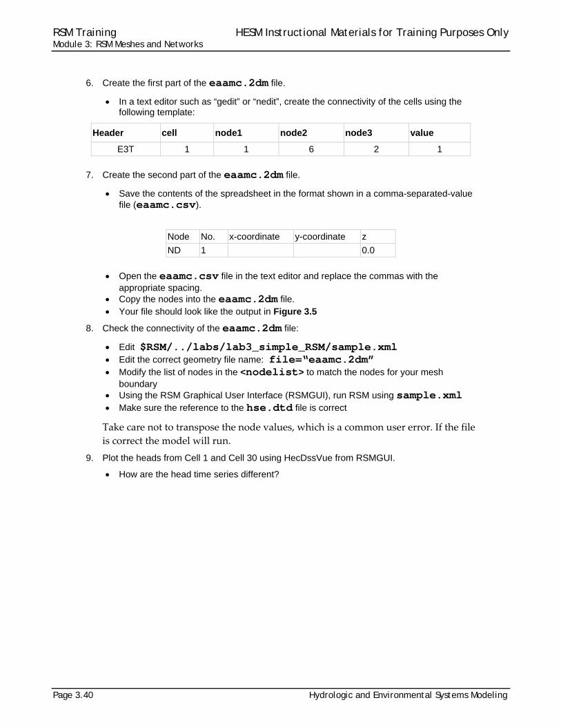
6. Create the first part of the eaamc.2dm file.

In a text editor such as “gedit” or “nedit”, create the connectivity of the cells using the following template:

Header cell node1 node2 node3 value

E3T 1 1 6 2 1

7. Create the second part of the eaamc.2dm file.

Save the contents of the spreadsheet in the format shown in a comma-separated-value file (eaamc.csv).

Node No. x-coordinate y-coordinate z

ND 1 0.0

Open the eaamc.csv file in the text editor and replace the commas with the

appropriate spacing. Copy the nodes into the eaamc.2dm file. Your file should look like the output in Figure 3.5

8. Check the connectivity of the eaamc.2dm file:

Edit $RSM/../labs/lab3_simple_RSM/sample.xml Edit the correct geometry file name: file=“eaamc.2dm” Modify the list of nodes in the <nodelist> to match the nodes for your mesh

boundary Using the RSM Graphical User Interface (RSMGUI), run RSM using sample.xml Make sure the reference to the hse.dtd file is correct

Take care not to transpose the node values, which is a common user error. If the file

is correct the model will run.

9. Plot the heads from Cell 1 and Cell 30 using HecDssVue from RSMGUI.

How are the head time series different?



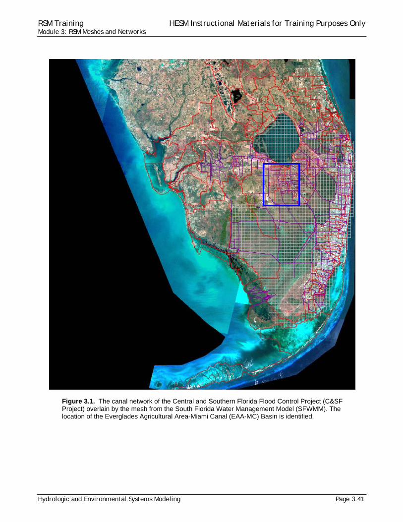
Figure 3.1. The canal network of the Central and Southern Florida Flood Control Project (C&SF Project) overlain by the mesh from the South Florida Water Management Model (SFWMM). The location of the Everglades Agricultural Area-Miami Canal (EAA-MC) Basin is identified.



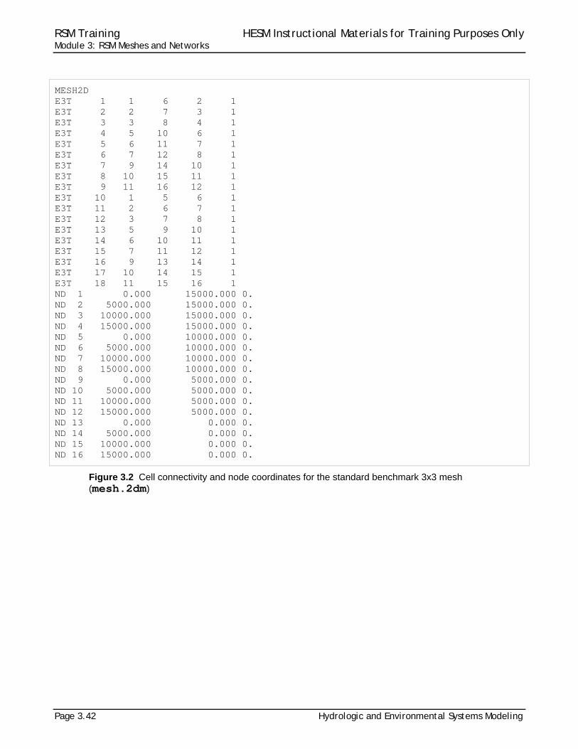
MESH2D E3T 1 1 6 2 1 E3T 2 2 7 3 1 E3T 3 3 8 4 1 E3T 4 5 10 6 1 E3T 5 6 11 7 1 E3T 6 7 12 8 1 E3T 7 9 14 10 1 E3T 8 10 15 11 1 E3T 9 11 16 12 1 E3T 10 1 5 6 1 E3T 11 2 6 7 1 E3T 12 3 7 8 1 E3T 13 5 9 10 1 E3T 14 6 10 11 1 E3T 15 7 11 12 1 E3T 16 9 13 14 1 E3T 17 10 14 15 1 E3T 18 11 15 16 1 ND 1 0.000 15000.000 0. ND 2 5000.000 15000.000 0. ND 3 10000.000 15000.000 0. ND 4 15000.000 15000.000 0. ND 5 0.000 10000.000 0. ND 6 5000.000 10000.000 0. ND 7 10000.000 10000.000 0. ND 8 15000.000 10000.000 0. ND 9 0.000 5000.000 0. ND 10 5000.000 5000.000 0. ND 11 10000.000 5000.000 0. ND 12 15000.000 5000.000 0. ND 13 0.000 0.000 0. ND 14 5000.000 0.000 0. ND 15 10000.000 0.000 0. ND 16 15000.000 0.000 0.

Figure 3.2 Cell connectivity and node coordinates for the standard benchmark 3x3 mesh (mesh.2dm)



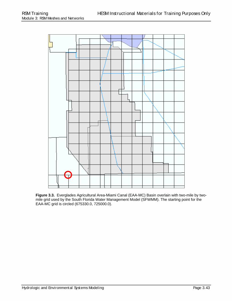
Figure 3.3. Everglades Agricultural Area-Miami Canal (EAA-MC) Basin overlain with two-mile by two-mile grid used by the South Florida Water Management Model (SFWMM). The starting point for the EAA-MC grid is circled (675330.0, 725000.0).



a) Locate 20-30 nodes in EAA-MC basin b) Create 20-30 acute triangular cells

c) Label the mesh cells

Figure 3.4 A simple irregular triangular mesh for the EAA-MC basin



MESH2D E3T 1 1 5 4 1 E3T 2 1 2 5 1 E3T 3 2 3 5 1 E3T 4 3 6 5 1 E3T 5 4 8 7 1 E3T 6 4 5 8 1 E3T 7 5 9 8 1 E3T 8 5 6 9 1 E3T 9 7 8 10 1 E3T 10 8 11 10 1 E3T 11 8 9 11 1 E3T 12 9 12 11 1 E3T 13 10 14 13 1 E3T 14 10 11 14 1 E3T 15 11 15 14 1 E3T 16 11 12 15 1 E3T 17 12 16 15 1 E3T 18 13 18 17 1 E3T 19 13 14 18 1 E3T 20 14 15 18 1 E3T 21 15 19 20 1 E3T 22 15 16 19 1 E3T 23 16 20 19 1 E3T 24 17 18 24 1 E3T 25 18 21 24 1 E3T 26 18 19 21 1 E3T 27 19 21 22 1 E3T 28 19 20 22 1 E3T 29 20 23 22 1 E3T 30 21 25 24 1 E3T 31 21 22 25 1 E3T 32 22 26 25 1 E3T 33 22 23 26 1 E3T 34 23 27 26 1 ND 1 685890.0 862280.0 0.0 ND 2 707010.0 862280.0 0.0 ND 3 728130.0 862280.0 0.0 ND 4 675330.0 841160.0 0.0 ND 5 707010.0 841160.0 0.0 ND 6 728130.0 841160.0 0.0 ND 7 675330.0 820040.0 0.0 ND 8 701730.0 820040.0 0.0 ND 9 728130.0 820040.0 0.0 ND 10 675330.0 798920.0 0.0 ND 11 707010.0 798920.0 0.0 ND 12 738690.0 798920.0 0.0 ND 13 675330.0 772520.0 0.0 ND 14 696450.0 777800.0 0.0 ND 15 714930.0 777800.0 0.0 ND 16 743970.0 777800.0 0.0 ND 17 675330.0 746120.0 0.0 ND 18 696450.0 756680.0 0.0 ND 19 717570.0 761960.0 0.0 ND 20 759810.0 761960.0 0.0 ND 21 720210.0 746120.0 0.0 ND 22 738690.0 746120.0 0.0 ND 23 759810.0 746120.0 0.0 ND 24 696450.0 725000.0 0.0 ND 25 722850.0 725000.0 0.0 ND 26 749250.0 725000.0 0.0 ND 27 775650.0 725000.0 0.0

Figure 3.5 The contents of the eaamc.2dm file for a simple mesh



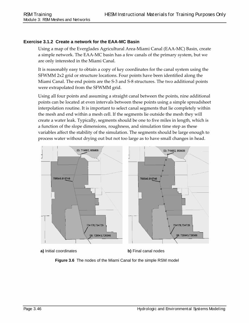
Exercise 3.1.2 Create a network for the EAA-MC Basin

Using a map of the Everglades Agricultural Area‐Miami Canal (EAA‐MC) Basin, create

a simple network. The EAA‐MC basin has a few canals of the primary system, but we

are only interested in the Miami Canal.

It is reasonably easy to obtain a copy of key coordinates for the canal system using the

SFWMM 2x2 grid or structure locations. Four points have been identified along the

Miami Canal. The end points are the S‐3 and S‐8 structures. The two additional points

were extrapolated from the SFWMM grid.

Using all four points and assuming a straight canal between the points, nine additional

points can be located at even intervals between these points using a simple spreadsheet

interpolation routine. It is important to select canal segments that lie completely within

the mesh and end within a mesh cell. If the segments lie outside the mesh they will

create a water leak. Typically, segments should be one to five miles in length, which is

a function of the slope dimensions, roughness, and simulation time step as these

variables affect the stability of the simulation. The segments should be large enough to

process water without drying out but not too large as to have small changes in head.

a) Initial coordinates b) Final canal nodes

Figure 3.6 The nodes of the Miami Canal for the simple RSM model



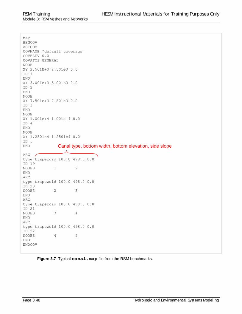
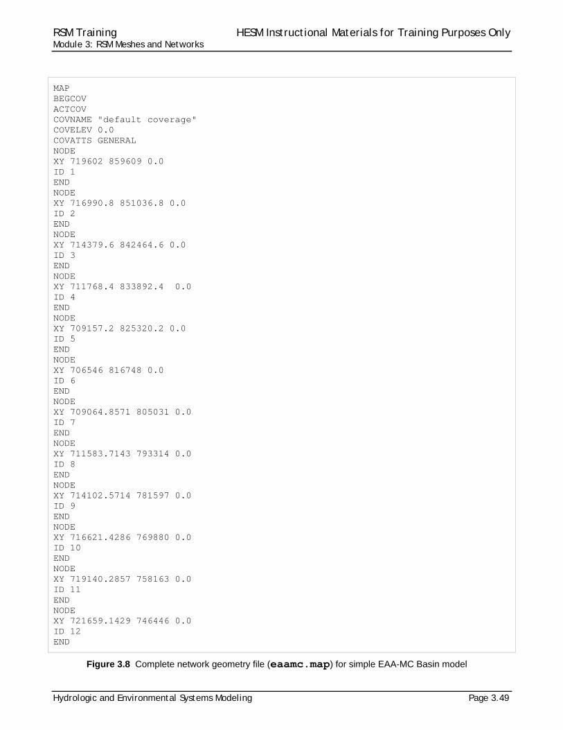
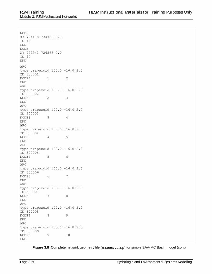
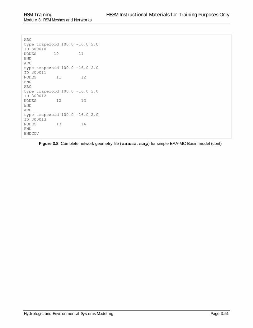
Once the coordinates of the canal nodes are obtained, create a canal *.map file using the example in Fig. 3.7 as an example. The *.map file is composed of two sections: the

node identification and the segment characteristics.

10. Create a node section using the x and y coordinates from the spreadsheet. Replace the x

and y values while retaining the remaining syntax.

11. Create the segment section by selecting segment ID values (beginning with the number

300001, so the segment waterbodies do not conflict with the cell waterbodies) and

determine the cross-section for each canal segment. The typical cross-section has a

trapezoidal profile followed by the bottom width, bottom elevation and side slope: type

trapezoid 100.0 498.0 0.0

The bottom elevation for the Miami Canal can be set to -16.0 feet for all segments. (The bottom elevation should be set sufficiently deep so that the canal never dries out during the simulation.)

The bottom width is 100 feet Sideslope is 2:1. The canal is relatively flat through the Everglades Agricultural Area.

12. Create a file “eaamc_canal.init” that contains the initial head for each canal

segment. The first line will have “netinit” and the remaining lines will have the head values

ordered by segment id, one value per line. Set all initial heads = “9.0”.

13. Create an “avcs.index” file to assign the appropriate segment (avc) definition to each

segment. In this example, there is only one avc type defined, “1”. The first six lines are

defined as the following with ND equal to the number of segments:

DATASET OBJTYPE “network” BEGSCL ND 13 NAME “segment index” TS 0 00

This is followed by a list of arc assignments ordered by segment id, one value per line.

14. Save the segment file as eaamc.map. The resulting file should look like the file in Fig.

3.8.

15. Using the RSMGUI, test the map file by running sample_eaa_net.xml.

16. Using HEC-DSSVue from the RSM GUI, plot the heads for cells 1, 7 and 30.

Why are the head time series different?



MAP BEGCOV ACTCOV COVNAME "default coverage" COVELEV 0.0 COVATTS GENERAL NODE XY 2.501E+3 2.501e3 0.0 ID 1 END XY 5.001e+3 5.001E3 0.0 ID 2 END NODE XY 7.501e+3 7.501e3 0.0 ID 3 END NODE XY 1.001e+4 1.001e+4 0.0 ID 4 END NODE XY 1.2501e4 1.2501e4 0.0 ID 5 END ARC type trapezoid 100.0 498.0 0.0 ID 19 NODES 1 2 END ARC type trapezoid 100.0 498.0 0.0 ID 20 NODES 2 3 END ARC type trapezoid 100.0 498.0 0.0 ID 21 NODES 3 4 END ARC type trapezoid 100.0 498.0 0.0 ID 22 NODES 4 5 END ENDCOV

Figure 3.7 Typical canal.map file from the RSM benchmarks.

Canal type, bottom width, bottom elevation, side slope



MAP BEGCOV ACTCOV COVNAME "default coverage" COVELEV 0.0 COVATTS GENERAL NODE XY 719602 859609 0.0 ID 1 END NODE XY 716990.8 851036.8 0.0 ID 2 END NODE XY 714379.6 842464.6 0.0 ID 3 END NODE XY 711768.4 833892.4 0.0 ID 4 END NODE XY 709157.2 825320.2 0.0 ID 5 END NODE XY 706546 816748 0.0 ID 6 END NODE XY 709064.8571 805031 0.0 ID 7 END NODE XY 711583.7143 793314 0.0 ID 8 END NODE XY 714102.5714 781597 0.0 ID 9 END NODE XY 716621.4286 769880 0.0 ID 10 END NODE XY 719140.2857 758163 0.0 ID 11 END NODE XY 721659.1429 746446 0.0 ID 12 END

Figure 3.8 Complete network geometry file (eaamc.map) for simple EAA-MC Basin model



NODE XY 724178 734729 0.0 ID 13 END NODE XY 729943 726366 0.0 ID 14 END

ARC type trapezoid 100.0 -16.0 2.0 ID 300001 NODES 1 2 END ARC type trapezoid 100.0 -16.0 2.0 ID 300002 NODES 2 3 END ARC type trapezoid 100.0 -16.0 2.0 ID 300003 NODES 3 4 END ARC type trapezoid 100.0 -16.0 2.0 ID 300004 NODES 4 5 END ARC type trapezoid 100.0 -16.0 2.0 ID 300005 NODES 5 6 END ARC type trapezoid 100.0 -16.0 2.0 ID 300006 NODES 6 7 END ARC type trapezoid 100.0 -16.0 2.0 ID 300007 NODES 7 8 END ARC type trapezoid 100.0 -16.0 2.0 ID 300008 NODES 8 9 END ARC type trapezoid 100.0 -16.0 2.0 ID 300009 NODES 9 10 END

Figure 3.8 Complete network geometry file (eaamc.map) for simple EAA-MC Basin model (cont)



ARC type trapezoid 100.0 -16.0 2.0 ID 300010 NODES 10 11 END ARC type trapezoid 100.0 -16.0 2.0 ID 300011 NODES 11 12 END ARC type trapezoid 100.0 -16.0 2.0 ID 300012 NODES 12 13 END ARC type trapezoid 100.0 -16.0 2.0 ID 300013 NODES 13 14 END ENDCOV

Figure 3.8 Complete network geometry file (eaamc.map) for simple EAA-MC Basin model (cont)





Answers for Lab 3:

Exercise 3.1.1 7. How are the head time series different?

The initial head for cell 1 is about 11.9 ft and drops to 10.1 ft by April, then goes

asymptotic to a head of 10.0 ft. The head in cell 30 quickly goes to 8.0 ft and then stays

constant throughout the run period.

Exercise 3.1.2 5. Why are the head time series different?

These time series are different because of the difference among the cell’s proximity to

the canal. The head in the canal is significantly lower than that of the cells so water

gradually seeps into the canal from the surrounding cells (this is a default

watermover). The closer the cell is to the edge of the canal, the more quickly and lower

the head will drop over time, as evidenced by the heads in these cells.





Index aquifer .................................................... 24 attribute 6, 7, 10, 12, 18, 19, 24, 25, 26, 36 automated tools ...................................... 37 basin ................................................. 44, 46 BBCW, see also Biscayne Bay Coastal

Wetlands ............................................. 38 benchmark . 3, 7, 12, 13, 18, 19, 36, 38, 39,

42, 48 BM16 .................................................. 19

bottom elevation ..................................... 47 C111 model ............................................ 38 canal ................................................. 20, 46

network ............................................... 41 segment ........................................ 46, 47

canal, see also WCD 20, 29, 32, 41, 46, 47, 48, 53

canal.map ............................................... 48 cell

connectivity ................................... 23, 39 ID .................................................. 36, 39

cell, see also mesh .. 21, 22, 23, 25, 26, 36, 39, 40, 42, 44, 46, 47, 53

coefficient ......................................... 24, 31 comma-separated-value file ................... 40 conductivity, see also hydraulic

conductivity ......................................... 24 control ................................................. 3, 18

block ................................................... 18 conveyance ................................ 24, 25, 36 coordinates ... 21, 22, 23, 29, 39, 42, 46, 47 coverage ........................................... 48, 49 default values ......................................... 12 distributed values .................................... 24 DSS time series file ................................ 18 DSSVue ...................................... 28, 40, 47 EAA . 20, 21, 29, 39, 41, 43, 44, 46, 49, 50,

51 EAA-MC basin ... 39, 41, 43, 44, 46, 49, 50,

51 EAA-MC model ................................. 39, 43 eaamc.2dm ....................................... 40, 45 eaamc.csv .............................................. 40 eaamc.map ........................... 47, 49, 50, 51 editors for Linux

gedit .................................................... 40 xemacs ..................................... 5, 7, 8, 9

environment variable .............................. 38 error ........................... 5, 6, 7, 12, 15, 36, 40 Everglades Agricultural Area 39, 41, 43, 46,

47 Everglades Agricultural Area-Miami Canal

(EAA-MC) Basin ................ 39, 41, 43, 46 FC, see also flood control ......................... 3 file format ............................................... 30

ASCII .............................................. 5, 39 DSS .................................................... 18 mesh.2dm ........................................... 39 NetCDF ............................................... 36 XML ....................... 17, 18, 19, 38, 40, 47

flood ......................................................... 3 flood control .............................................. 3 flow ............................................. 10, 24, 31 geodatabase .......................................... 25 geographic data ..................................... 26 GMS ...................................... 23, 30, 36, 39

format ........................................... 23, 36 grep ........................................................ 13 groundwater ........................................... 24

flow ..................................................... 24 gw, see groundwater ................................ 5 head .......................... 24, 31, 40, 46, 47, 53 historical data ................................... 14, 32 Holeyland ............................................... 39 how to

build a simple RSM ....................... 15, 37 complete network geometry file ... 49, 50,

51 create a node section ......................... 47 create a simple network ...................... 46 create the segment section ................. 47 obtain a copy of key coordinates for the

canal system using the SFWMM 2x2 grid .................................................. 46

HPM ...................................... 27, 28, 36, 38 water budget ................................. 28, 38

HSE ........................... 2, 3, 7, 11, 12, 19, 36 hse.dtd file ......... 5, 6, 7, 8, 9, 10, 12, 36, 40 Hydrologic Simulation Engine, see also

HSE .................................................... 18 indexed entry, see also HPM ................. 25 initial head .................................. 31, 47, 53 Initial head .............................................. 24



input data ................................................ 18 boundary conditions .... 14, 18, 31, 32, 36 canals ................................................. 47 mesh ....................................... 37, 39, 42

input files .................................... 15, 17, 33 map file ....................... 30, 35, 36, 47, 48 necessary ............................................ 37

key coordinates for the canal system ..... 46 landuse ............................................. 20, 25 Linux ............................................... 5, 7, 13 main XML file ............................................ 6 make, see makefile ........................... 11, 30 Management Simulation Engine, see also

MSE .................................................... 11 marsh, see also HPM - layer1nsm .......... 20 mesh .. 7, 10, 14, 19, 21, 22, 23, 24, 26, 35,

36, 37, 39, 40, 41, 42, 44, 45, 46 geometry ............................................. 23 node ... 21, 22, 23, 29, 30, 36, 39, 40, 42,

44, 46, 47 mesh and network ............................ 37, 39 metadata ................................................ 26 Miami Canal........ 20, 21, 29, 41, 43, 46, 47 model input, see input data .................... 36 model output, see output data ................ 14 monitor ....................................... 10, 28, 36

global .................................................. 28 network .. 14, 19, 22, 29, 30, 31, 36, 37, 39,

41, 46, 47, 49, 50, 51 network file ............................................. 37 network geometry ........... 30, 31, 49, 50, 51 node coordinate location section ............ 39 node id .............................................. 39, 47 node identification ................................... 47 note .................................................... 2, 38 output data ..... 3, 10, 14, 19, 28, 35, 36, 40

water budget ....................................... 28 output elements ...................................... 19 overbank flow ......................................... 31 parameter ................. 3, 5, 6, 12, 13, 36, 39 performance measures ..................... 14, 15 plot .................................................... 40, 47 primary system ....................................... 46 pump, see also watermover.................... 29 rainfall ..................................................... 38 reference

HSE User Manual ................. 2, 3, 12, 36

Regional Simulation Model, see also RSM........................................................ 1, 37

Rotenberger ..................................... 20, 39 RSM

implementation ... 3, 5, 11, 15, 18, 19, 32, 33, 35, 36, 37

RSM GUI .......................................... 40, 47 GIS ToolBar ............................ 19, 33, 37 toolbar ..................................... 28, 40, 47

RSM, see also Regional Simulation Model 1, 2, 3, 5, 6, 7, 10, 11, 12, 13, 14, 15, 16, 17, 18, 19, 27, 28, 32, 33, 35, 36, 37, 38, 39, 40, 46, 47, 48

rulecurve ................................................ 10 run3x3.xml .............................................. 19 runDescriptor .......................................... 18 sample.xml ................................. 17, 38, 40 sample_eaa_net.xml .............................. 47 scrub land, see also HPM ...................... 20 seepage ................................................. 31 segment

attributes ....................................... 31, 47 head .................................................... 31 ID values ............................................. 47

segment, see also waterbody segment ....................... 31, 32, 36, 46, 47

setenv ..................................................... 38 SFWMM .............. 21, 22, 29, 39, 41, 43, 46

grid ..................................... 22, 29, 39, 46 simple boundary conditions .................... 32 soil .......................................................... 25 source code ......................... 6, 7, 12, 13, 36 South Florida Water Management Model,

see also SFWMM .............. 21, 39, 41, 43 spatial input files ..................................... 37 stage ...................................................... 24 stage-volume .......................................... 24 standard mesh format ............................ 39 structure ................ 5, 10, 14, 15, 29, 32, 46

locations ....................................... 29, 46 S3 ........................................... 20, 29, 46 S8 ........................................... 20, 29, 46

subregional models .................3, 12, 32, 37 sugarcane .............................................. 20 surface elevation .................................... 24 surface hydrology ................................... 27 SVconverter ..................................... 24, 25 template ................................................. 40



testbed .................................................... 13 time series .......... 10, 18, 28, 32, 40, 47, 53 time step ..................................... 18, 28, 46 topography ........................... 25, 26, 27, 35 transmissivity .............................. 24, 25, 36 typical cross-section ............................... 47 uncertainty .............................................. 14 utilities .................................................... 28 volume .................................................... 24 water supply ............................................. 3

waterbody ................................... 11, 28, 47 segment .............................................. 47

watermover ............................................ 53 well ........................................ 10, 14, 16, 23 WS, see also water supply ....................... 3 x-coordinate ..................................... 39, 40 x-y-z coordinates .................................... 39 y-coordinate ..................................... 39, 40 z-axis ...................................................... 39 zero-coordinate value ............................. 39



Documents

Build a simple RSM-HSE · RSM Training HESM Instructional Materials for Training Purposes Only Module 3: RSM Meshes and Networks Hydrologic and Environmental Systems Modeling Page