Bursting of Morris-Lecar neuronal model with current-feedback control

Science in China Series E: Technological Sciences

© 2009 SCIENCE IN CHINA PRESS

Springer

Sci China Ser E-Tech Sci | Mar. 2009 | vol. 52 | no. 3 | 771-781

www.scichina.com tech.scichina.com

www.springerlink.com

Bursting of Morris-Lecar neuronal model with current-feedback control

DUAN LiXia1, LU QiShao2† & CHENG DaiZhan3 1 College of Science, North China University of Technology, Beijing 100144, China; 2 School of Science, Beijing University of Aeronautics and Astronautics, Beijing 100191, China; 3 Institute of Systems Science, Chinese Academy of Sciences, Beijing 100190, China

The Morris-Lecar (ML) neuronal model with current-feedback control is considered as a typical fast-slow dynamical system to study the combined influences of the reversal potential VCa of Ca2+ and the feedback current I on the generation and transition of different bursting oscillations. Two-parameter bifurcation analysis of the fast subsystem is performed in the parameter (I, VCa)-plane at first. Three important codimension-2 bifurcation points and some codimension-1 bifurcation curves are obtained which enable one to determine the parameter regions for different types of bursting. Next, we further divide the control parameter (V0, VCa)-plane into five different bursting regions, namely, the “fold/fold” bursting region R1, the “fold/Hopf” bursting region R2, the “fold/homoclinic” bursting region R3, the “subHopf/homoclinic” bursting region R4 and the “subHopf/subHopf” bursting region R5, as well as a silence region R6. Codimension-1 and -2 bifurcations are responsible for explanation of transition mechanisms between different types of bursting. The results are instructive for further understanding the dynamical behavior and mechanisms of complex firing activities and information processing in biological nervous systems.

neuron, bursting, bifurcation, fast-slow dynamics analysis, codimension

1 Introduction

Nerve cells (neurons) are responsible for receiving and transmitting signals to and from the Central Nervous System. Neural information is encoded and transmitted as spikes in membrane electrical potential, called action potentials. One of the major challenges in neuroscience is to understand the basic physiological mechanisms underlying the complex spatiotemporal patterns of spik-ing activity observed during the normal functioning of the brain, and to determine the origins of pathological dynamical states such as epilepsy, Parkinson’s disease, Alzheimer’s disease, and schizophrenia. A second major challenge is to understand how the patterns of spiking activity provide a substrate for the encoding and trans-mission of information.

A common variety of firing in neurons and other ex-citable cells is bursting oscillation. Bursting is a rela-

tively slow rhythmic alternation between an active phase of rapid spiking and a quiescent phase without spiking. It occurs in many nerve and endocrine cells, including thalamic neurons, hypothalamic neurons, pyramidal neurons in the neocortex, respiratory neurons in pre-Bötzinger complex, pituitary cells, and pancreatic β -cells. There are several possible physiological roles of bursting, such as bursting can overcome synaptic transmission failure, facilitate transmitter release, and evoke long-term potentiation and hence affect synaptic plasticity much greater, or differently than single spikes[1]. In addition, bursting have more informational content than single spikes when analyzed as unitary Received October 20, 2008; accepted November 12, 2008 doi: 10.1007/s11431-009-0040-5 †Corresponding author (email: [email protected]) Supported by the National Natural Science Foundation of China (Grant Nos. 10872014 and 10702002)

772 DUAN LiXia et al. Sci China Ser E-Tech Sci | Mar. 2009 | vol. 52 | no. 3 | 771-781

events[2] and have higher signal-to-noise ratio than single spikes[3]. It has been proposed to provide effective mechanisms for selective communication between neurons[4]. So the understanding of how bursting activities can be generated and transmitted among neurons is of fundamental importance.

The firing activities change according to certain bi-furcation principles. Hence the bifurcation scenarios among various firing activities are fundamental to the study of neural bursting. The fast-slow dynamics analysis developed by Rinzel and collaborators provided a general framework for understanding the biophysical origins of bursting by mathematical models and compu- tations[5]. Bursting oscillations in the models of neurons and other excitable cells have been studied extensively. For example, A rigorous mathematical treatment of aspects of the generation of spiking and bursting and transition between them was provided[6―8]. Belykh et al.[9] pre- sented four different dynamic scenarios for the emergence of bursting. Guckenheimer and Tien[10] investigated the relationship between transitions in several bursting models with bifurcations of reduced subsystem. The emergence of different types of bursting in various neuronal models was investigated[11―16]. Shorten and Wall[11] found different modes of bursting oscillations in a Hodgkin-Huxley type neuronal model and investigate mode transitions and similar modes of bursting in other models. They used bifurcation analysis and null-surfaces to facilitate a geometric interpretation of bursting modes. Bertram et al.[12] studied some bursting oscillations in the Chay-Cook neuronal model by using two-parameter bifurcation analysis. Xie et al.[13] clarified the role of veratridine and the reason for the emergence of parabolic bursting in experiments by using the Plant model to account for the mechanism for parabolic bursting. Yang and Lu[14] investigated different types of bursting in the Chay neuronal model by fast-slow dynamics analysis. Channell et al.[15] pointed out that the incre- mental spike adding cascade in the reduced oscillatory heart interneuron model is attested to be caused by the homoclinic bifurcations of a saddle periodic orbit, set- ting the threshold between the tonic spiking and quiescent phases of the bursting. Furthermore, the origin and transition of bursting in coupled neuronal networks have gained extensive attention in recent years[16, 17]. Most of these studies were confined to investigating the generation mechanisms of firing patterns at individual parame-

ter or continuous mode transitions under single-parameter control. Since neuronal activities are influenced by many factors, now it is important and interesting to study what the neuron model would exhibit under the control of mul-tiple parameters and how we can determine the parameter regions for different electrical activities.

In our previous work[18], we applied the bifurcation theory and fast-slow dynamics analysis to the Chay model to analyze the variation of firing activities by continuously changing the value of a single parameter. As is well known, the Morris-Lecar (ML) neuronal model[19], which grew out of an experimental study of the excitability of giant muscle fiber of the huge Pacific barnacle, is one of favorite conductance-based models in computational neuroscience. In this paper, based on Rinzel’s fast-slow dynamics analysis[5] and the Izhike-vich’s classification scheme of bursting[20], two-parameter bifurcation analysis is utilized to gain a deeper insight into the combined influences of the reversal potential VCa of Ca2+ and the feedback current I on the generation and transition of different bursting oscillations of the ML model with current-feedback. Although some two-parameter bifurcation analysis of firing activities of the ML model was made by Tsumoto and Kitajima[21], detailed study on bursting of the ML model with current- feedback under the control of multiple parameters still has not been investigated.

This paper is organized as follows. In Section 2, we briefly describe the ML model with the current-feedback control. The influences of both the reversal potential of Ca2+ and the feedback current on the neuronal bursting oscillations are investigated in Sections 3 and 4. Section 5 shows that the control parameter (V0, VCa)-plane can be divided into five different bursting regions as well as a silence region. Conclusions are given in the last section.

2 Model description

The two-variable ML neuronal model consists of the voltage-gated Ca2+ current, the voltage-gated delayed- rectifier K+ current, and the leakage current. The equa-tions of the ML model are given as follows:

Ca Ca K K L Ld ( )( ) ( ) ( ) ,dVC g m V V V g w V V g V V It ∞= − + − + − +

(1)

( )d ,

d ( )w

w V wwt V

φτ

∞ −= (2)

DUAN LiXia et al. Sci China Ser E-Tech Sci | Mar. 2009 | vol. 52 | no. 3 | 771-781 773

where the gating functions are

1 2( ) 0.5(1 tanh(( ) / ),m V V V V∞ = + −

3 4( ) 0.5(1 tanh(( ) / ),w V V V V∞ = + − 1

3 4( ) (1 cosh(( ) / 2 ) .w V V V Vτ −= + −

In eqs. (1) and (2), variables V and w represent the membrane voltage and the activation of delayed rectifier K+ current, respectively. The parameters gCa, gK and gL are the maximal conductances associated with the three transmembranar currents; VCa, VK, and VL are the corre-sponding reversal potentials. The constant φ determines the scaling of the rate for K+ channel opening. Now we take the input current I as a linear feedback control sat-isfying

0d ( ),dI V Vt

ε= − (3)

where ε serves as a feedback coefficient and we take ε = 0.001 in the following computation, V0 is a contro-lable parameter. Eqs. (1)―(3) are called the ML model with current-feedback control (abbreviated as MLF model below). Because the gating functions are de-pendent on the membrane voltage V nonlinearly, there exists complex nonlinear dynamical behavior in this MLF model.

The mathematics mechanisms of bursting can be de-scribed as the interaction of two subsystems dynamically separated by their intrinsic time scales: A faster subsystem typically governed by sodium and potassium channels, which can either be at rest or exhibit repetitive spikes, and a slow subsystem driving the fast one through its quies-cent and oscillatory states in a quasi-static manner[22]. The slow-varying dynamics mechanism can be attrib-uted to the accumulation of intracellular calcium ions or other slow voltage-dependent processes[20, 23]. Since ε is small, the feedback current I in eq. (3), which is consid-ered as a slow voltage-dependent variable of the whole MLF model, controls the dynamics of the fast subsystem eqs. (1) and (2) and then can be considered as a bifurca-tion parameter of the fast subsystem.

Bursting oscillations can be influenced by many fac-tors, such as outward input current, the ionic currents (typically, that of sodium (Na+), potassium (K+) and cal-cium (Ca2+)) through the cell membrane, and so on. Of-tentimes, Ca2+ has very important effects on the nerve system. The dynamical nature of abundant bursting patterns under the control of multiple parameters is related

to neuronal calcium activities and is worth further inves-tigation. On the other hand, some types of neurons are able to respond to the current input by emitting an all- or non-burst response. In this paper, we will investigate the influence of both the reversal potential of Ca2+ (that is, VCa) and the feedback current (consider the parameter V0) on the creation and transition mechanisms of different bursting oscillations. The parameter values used here are: VK = −84 mV, VL = −60 mV, gK = 8 μF/cm2, gCa = 4 μS/cm2, gL = 2 μF/cm2, C = 20 μF/cm2, V1 = −1.2 mV, V2 = 18 mV, V3 = 12 mV, V4 = 17.4 mV and φ = 0.23. This model was solved by using a stiff system solver in the numerical package XPPAUT[24]. The bifurcation diagrams were computed by using AUTO as incorporated in XPPAUT.

3 Two-parameter bifurcation analysis for V0=−22 mV

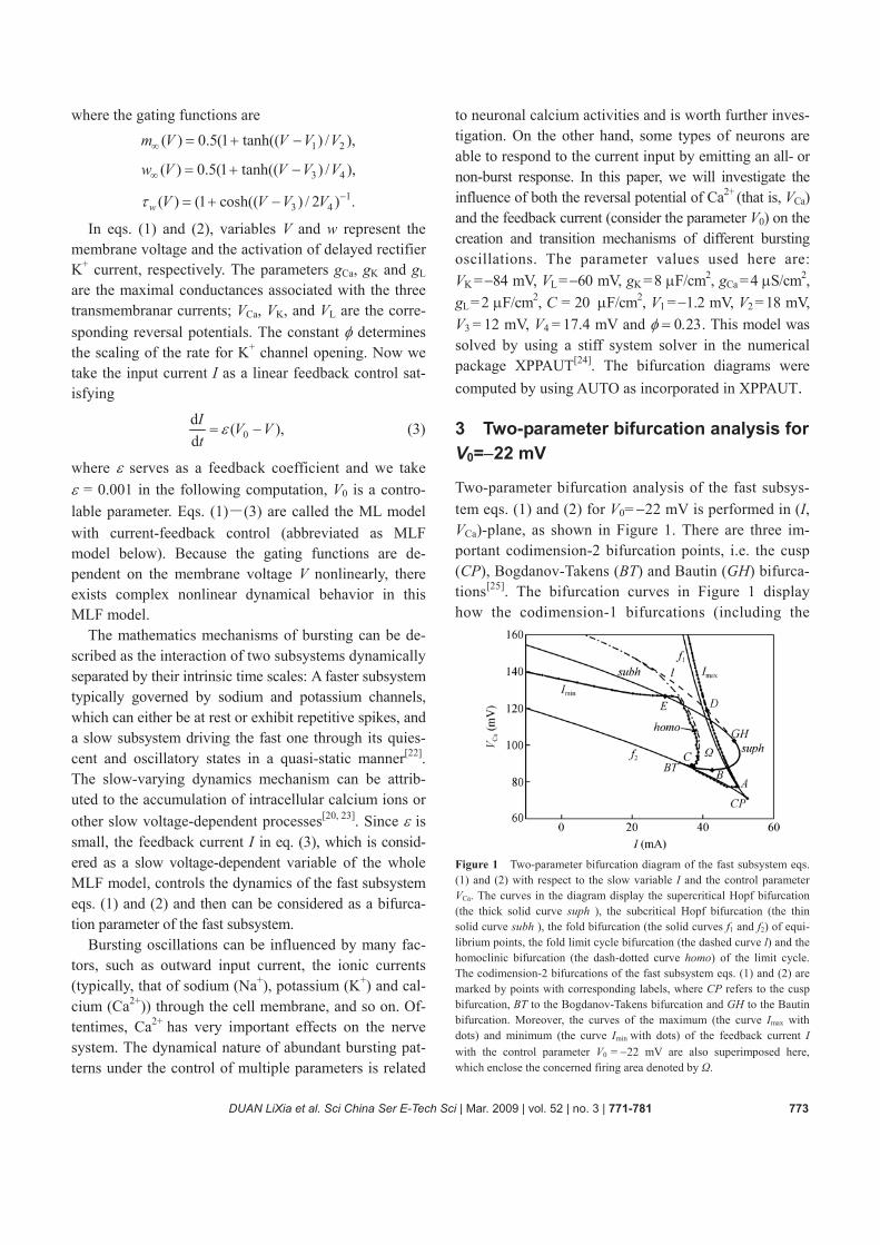
Two-parameter bifurcation analysis of the fast subsys-tem eqs. (1) and (2) for V0= −22 mV is performed in (I, VCa)-plane, as shown in Figure 1. There are three important codimension-2 bifurcation points, i.e. the cusp (CP), Bogdanov-Takens (BT) and Bautin (GH) bifurcations[25]. The bifurcation curves in Figure 1 display how the codimension-1 bifurcations (including the

Figure 1 Two-parameter bifurcation diagram of the fast subsystem eqs. (1) and (2) with respect to the slow variable I and the control parameter VCa. The curves in the diagram display the supercritical Hopf bifurcation (the thick solid curve suph ), the subcritical Hopf bifurcation (the thin solid curve subh ), the fold bifurcation (the solid curves f1 and f2) of equi-librium points, the fold limit cycle bifurcation (the dashed curve l) and the homoclinic bifurcation (the dash-dotted curve homo) of the limit cycle. The codimension-2 bifurcations of the fast subsystem eqs. (1) and (2) are marked by points with corresponding labels, where CP refers to the cusp bifurcation, BT to the Bogdanov-Takens bifurcation and GH to the Bautin bifurcation. Moreover, the curves of the maximum (the curve Imax with dots) and minimum (the curve Imin with dots) of the feedback current I with the control parameter V0 = −22 mV are also superimposed here, which enclose the concerned firing area denoted by Ω.


subcritical Hopf (subh), supercritical Hopf (suph), fold (f1 and f2) bifurcations of equilibrium points, the fold limit cycle (l) and homoclinic (homo) bifurcations of limit cycles) vary with the parameters. Taking into ac-count that the presence of slow oscillations is a neces-sary condition for bursting, the dynamical behavior of the slow subsystem eq. (3) is also discussed corre-spondingly. The curves of the maximum (Imax) and minimum (Imin) of the feedback current I are also su-perimposed here. For certain values of VCa, the feedback current I varies between the curves of Imin and Imax, which enclose the firing area denoted by Ω. The transi-tions between different bursting are mainly determined by the bifurcations happening in Ω.

The fold bifurcation curves f1 and f2 are composed of equilibrium points with a simple zero eigenvalue λ = 0 and no other eigenvalue on the imaginary axis. In gen-eral, the restriction of the fast subsystem eqs. (1) and (2) to the one-dimensional center manifold for the points on f1 and f2 has the normal form

2 3(| | ),a Οξ ξ ξ= + 1.Rξ ∈ (4)

When the parameters I and VCa change, the fold bifurca-tion curves f1 and f2 meet tangentially at the codimen-sion-2 cusp bifurcation point CP (52.6030, 70.9883), where the eigenvalues are λ1 = 0, λ2 = −0.2167. It is seen that λ1 = 0 remains a simple eigenvalue and is the only one on the imaginary axis at the point CP. However, the normal form coefficient a in eq. (4) vanishes at point CP, that is, a =0, and then the restriction of the subsystem eqs. (1) and (2) to the center manifold has the normal form

3 4(| | ),c Οξ ξ ξ= + 1,Rξ ∈

where c = −0.00034 (computed by the package con-tent[26]). Near the point CP, the fast subsystem eqs. (1) and (2) is locally topologically equivalent to the normal form

31 2

1 1

,,

ξ β β ξ σξη η− −

⎧ = + +⎪⎨

= −⎪⎩

where σ = sign(c)=−1, η−1∈R1, β1, β2∈R. With the parameters changing further, a codimen-

sion-2 Bogdanov-Takens bifurcation takes place at the point BT (33.5162, 90.4477) with two eigenvalues λ1,2 = 0. The fast subsystem eqs. (1) and (2) near BT is locally topologically equivalent to the normal form

1 22

2 1 2 1 1 1 2

,

,s

η η

η β β η η η η

=⎧⎪⎨

= + + +⎪⎩

where a = 0.00303, b = −0.01132 (computed by content[26]), s = sign(ab)= −1. The point BT is a tangency point of the supercritical Hopf bifurcation curve (suph) and the fold bifurcation curve (f2) of the equilibrium points. At the same time, a homoclinic curve (homo) emanates from the point BT[25], as shown in Figure 1.

A codimension-2 Bautin bifurcation takes place at the point GH (48.8497, 102.4096) with a pair of complex conjugate eigenvalues λ1,2 = ±0.3317ω, and the first Lyapunov coefficient vanishes: l1=0. The fast subsystem eqs. (1) and (2) is near GH locally topologically equiva-lent to the normal form

2 41 2( ) | | | | ,z i z z z sz zβ β= + + + 1,z C∈

where s=sign(l2), l2 is the second Lyapunov coefficient. The values of VCa at some points in Figure 1 are listed

here for further discussion. The whole system starts fir-ing at the point A with VCa = VCa (A)=77.2253 mV; the point B corresponds to the minimal value of VCa for supercritical Hopf bifurcation with VCa = VCa (B)=86.5675 mV; the point C corresponds to the minimal value of VCa for the homoclinic bifurcation at which VCa = VCa (C)= 89.1005 mV; the point D is the intersection of the curves l and Imax at VCa = VCa (D)=118.8441 mV. The point E is the intersection of the curves subh and Imix at VCa = VCa (E)=127.2796 mV.

3.1 Transition from subthreshold oscillation to “fold/ fold” bursting

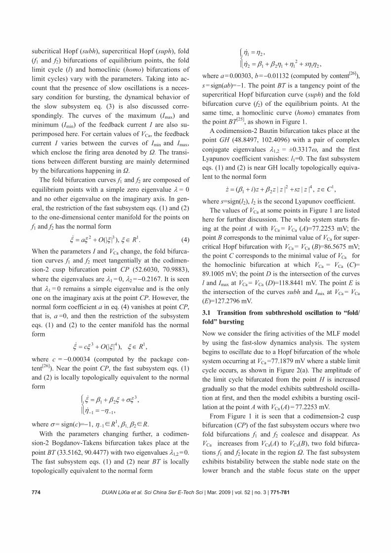
Now we consider the firing activities of the MLF model by using the fast-slow dynamics analysis. The system begins to oscillate due to a Hopf bifurcation of the whole system occurring at VCa =77.1879 mV where a stable limit cycle occurs, as shown in Figure 2(a). The amplitude of the limit cycle bifurcated from the point H is increased gradually so that the model exhibits subthreshold oscillation at first, and then the model exhibits a bursting oscillation at the point A with VCa (A) = 77.2253 mV.

From Figure 1 it is seen that a codimension-2 cusp bifurcation (CP) of the fast subsystem occurs where two fold bifurcations f1 and f2 coalesce and disappear. As VCa increases from VCa(A) to VCa(B), two fold bifurca-tions f1 and f2 locate in the region Ω. The fast subsystem exhibits bistability between the stable node state on the lower branch and the stable focus state on the upper


Figure 2 (a) Bifurcation diagram of the MLF mode eqs. (1)―(3) with respect to the parameter VCa. The stable steady states (the solid curves) become unstable (the dashed curve) and the stable limit cycles occur at the supercritical Hopf bifurcation (H). Vmax and Vmin represent the maximal and minimal values of the membrane potential V, respectively. (b1) Subthreshold oscillation for VCa =77.20 mV, (b2) the fast-slow dynamic bifurcation analysis for VCa

=77.20 mV. The upper and lower branches (the solid curves) of the Z-shaped curve are stable focuses and nodes, respectively, and the middle branch (the dashed curve) is composed of saddles. The trajectory of the MFL model eqs. (1)―(3) is also superimposed. (c1) Bursting oscillation for VCa =77.2253 mV, (c2) the fast-slow dynamic bifurcation analysis for VCa =77.2253 mV. The description of the curves and points is the same as that in (b1).

branch of the Z-shaped curve. So the model is capable of “fold/fold” bursting, as shown in Figures 2(c2) and 3. It should be remarked that if VCa is less than 77.2253 mV, the model behaves in a subthreshold oscillation state (shown in Figure 2(b1)) or a quiescent state and incapa-ble of bursting.

Figure 3(b) is the fast-slow dynamics analysis for the “fold/fold” bursting via point-point hysteresis loop in the

(I, V)-phase plane for VCa = 84.5 mV. The main charac-teristic of the point-point bursting is that the quiescent state disappears via a fold bifurcation and the firing state disappears via another fold bifurcation in the fast sub-system. The fast subsystem does not have a limit cycle attractor for any value of the slow variable. Bursting occurs owing to the rate of convergence to the upper state is relatively weak.


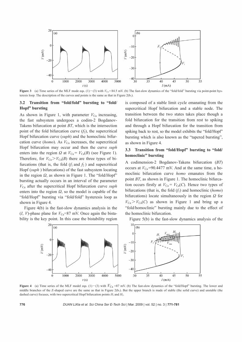
Figure 3 (a) Time series of the MLF mode eqs. (1)―(3) with VCa = 84.5 mV. (b) The fast-slow dynamics of the “fold/fold” bursting via point-point hys-teresis loop. The description of the curves and points is the same as that in Figure 2(b1).

3.2 Transition from “fold/fold” bursting to “fold/ Hopf” bursting As shown in Figure 1, with parameter VCa increasing, the fast subsystem undergoes a codim-2 Bogdanov- Takens bifurcation at point BT, which is the intersection point of the fold bifurcation curve (f2), the supercritical Hopf bifurcation curve (suph) and the homoclinic bifur-cation curve (homo). As VCa increases, the supercritical Hopf bifurcation may occur and then the curve suph enters into the region Ω at VCa = VCa(B) (see Figure 1). Therefore, for VCa＞VCa(B) there are three types of bi-furcations (that is, the fold (f1 and f2 ) and supercritical Hopf (suph ) bifurcations) of the fast subsystem locating in the region Ω, as shown in Figure 1. The “fold/Hopf” bursting actually occurs in an interval of the parameter VCa after the supercritical Hopf bifurcation curve suph enters into the region Ω, so the model is capable of the “fold/Hopf” bursting via “fold/fold” hysteresis loop as shown in Figure 4.

Figure 4(b) is the fast-slow dynamics analysis in the (I, V)-phase plane for VCa = 87 mV. Once again the bista-bility is the key point. In this case the bistability region

is composed of a stable limit cycle emanating from the supercritical Hopf bifurcation and a stable node. The transition between the two states takes place though a fold bifurcation for the transition from rest to spiking and through a Hopf bifurcation for the transition from spiking back to rest, so the model exhibits the “fold/Hopf” bursting which is also known as the “tapered bursting”, as shown in Figure 4. 3.3 Transition from “fold/Hopf” bursting to “fold/ homoclinic” bursting A codimension-2 Bogdanov-Takens bifurcation (BT) occurs at VCa =90.4477 mV. And at the same time, a ho-moclinic bifurcation curve homo emanates from the point BT, as shown in Figure 1. The homoclinic bifurca-tion occurs firstly at VCa = VCa(C). Hence two types of bifurcations (that is, the fold (f1) and homoclinic (homo) bifurcations) locate simultaneously in the region Ω for VCa＞VCa(C) as shown in Figure 1 and bring up a “fold/homoclinic” bursting mainly due to the effect of the homoclinic bifurcation.

Figure 5(b) is the fast-slow dynamics analysis of the

Figure 4 (a) Time series of the MLF model eqs. (1)―(3) with VCa =87 mV. (b) The fast-slow dynamics of the “fold/Hopf” bursting. The lower and middle branches of the Z-shaped curve are the same as that in Figure 2(b1). But the upper branch is made of stable (the solid curve) and unstable (the dashed curve) focuses, with two supercritical Hopf bifurcation points H1 and H2.


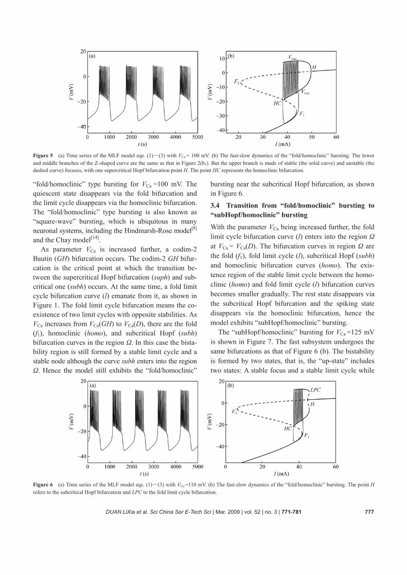
Figure 5 (a) Time series of the MLF model eqs. (1)―(3) with VCa = 100 mV. (b) The fast-slow dynamics of the “fold/homoclinic” bursting. The lower and middle branches of the Z-shaped curve are the same as that in Figure 2(b1). But the upper branch is made of stable (the solid curve) and unstable (the dashed curve) focuses, with one supercritical Hopf bifurcation point H. The point HC represents the homoclinic bifurcation.

“fold/homoclinic” type bursting for VCa =100 mV. The quiescent state disappears via the fold bifurcation and the limit cycle disappears via the homoclinic bifurcation. The “fold/homoclinic” type bursting is also known as “square-wave” bursting, which is ubiquitous in many neuronal systems, including the Hindmarsh-Rose model[8] and the Chay model[14].

As parameter VCa is increased further, a codim-2 Bautin (GH) bifurcation occurs. The codim-2 GH bifur-cation is the critical point at which the transition be-tween the supercritical Hopf bifurcation (suph) and sub-critical one (subh) occurs. At the same time, a fold limit cycle bifurcation curve (l) emanate from it, as shown in Figure 1. The fold limit cycle bifurcation means the co-existence of two limit cycles with opposite stabilities. As VCa increases from VCa(GH) to VCa(D), there are the fold (f1), homoclinic (homo), and subcritical Hopf (subh) bifurcation curves in the region Ω. In this case the bista-bility region is still formed by a stable limit cycle and a stable node although the curve subh enters into the region Ω. Hence the model still exhibits the “fold/homoclinic”

bursting near the subcritical Hopf bifurcation, as shown in Figure 6.

3.4 Transition from “fold/homoclinic” bursting to “subHopf/homoclinic” bursting

With the parameter VCa being increased further, the fold limit cycle bifurcation curve (l) enters into the region Ω at VCa = VCa(D). The bifurcation curves in region Ω are the fold (f1), fold limit cycle (l), subcritical Hopf (subh) and homoclinic bifurcation curves (homo). The exis-tence region of the stable limit cycle between the homo-clinic (homo) and fold limit cycle (l) bifurcation curves becomes smaller gradually. The rest state disappears via the subcritical Hopf bifurcation and the spiking state disappears via the homoclinic bifurcation, hence the model exhibits “subHopf/homoclinic” bursting.

The “subHopf/homoclinic” bursting for VCa =125 mV is shown in Figure 7. The fast subsystem undergoes the same bifurcations as that of Figure 6 (b). The bistability is formed by two states, that is, the “up-state” includes two states: A stable focus and a stable limit cycle while

Figure 6 (a) Time series of the MLF model eqs. (1)―(3) with VCa =110 mV. (b) The fast-slow dynamics of the “fold/homoclinic” bursting. The point H refers to the subcritical Hopf bifurcation and LPC to the fold limit cycle bifurcation.


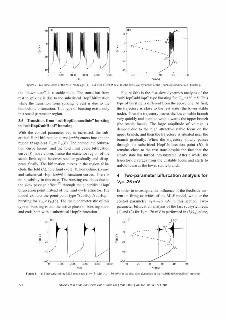
Figure 7 (a) Time series of the MLF mode eqs. (1)―(3) with VCa =125 mV; (b) the fast-slow dynamics of the “ subHopf/homoclinic” bursting.

the “down-state” is a stable node. The transition from rest to spiking is due to the subcritical Hopf bifurcation while the transition from spiking to rest is due to the homoclinic bifurcation. This type of bursting exists only in a small parameter region.

3.5 Transition from “subHopf/homoclinic” bursting to “subHopf/subHopf” bursting

With the control parameter VCa is increased, the sub-critical Hopf bifurcation curve (subh) enters into the the region Ω again at VCa = VCa(E). The homoclinic bifurcation curve (homo) and the fold limit cycle bifurcation curve (l) move closer, hence the existence region of the stable limit cycle becomes smaller gradually and disappears finally. The bifurcation curves in the region Ω in- clude the fold (f1), fold limit cycle (l), homoclinic (homo) and subcritical Hopf (subh) bifurcation curves. There is no bistability in this case. The bursting oscillates due to the slow passage effect[27] through the subcritical Hopf bifurcation point instead of the limit cycle attractor. The model exhibits the point-point type “subHopf/subHopf” bursting for VCa＞VCa(E). The main characteristic of this type of bursting is that the active phase of bursting starts and ends both with a subcritical Hopf bifurcation.

Figure 8(b) is the fast-slow dynamics analysis of the “subHopf/subHopf” type bursting for VCa =130 mV. This type of bursting is different from the above one. At first, the trajectory is close to the rest state (the lower stable node). Then the trajectory passes the lower stable branch very quickly and starts to wrap towards the upper branch (the stable focus). The large amplitude of voltage is damped due to the high attractive stable focus on the upper branch, and then the trajectory is situated near the branch gradually. When the trajectory slowly passes through the subcritical Hopf bifurcation point (H), it remains close to the rest state despite the fact that the steady state has turned into unstable. After a while, the trajectory diverges from the unstable focus and starts to unfold towards the lower stable branch.

4 Two-parameter bifurcation analysis for V0=−26 mV

In order to investigate the influence of the feedback cur-rent on firing activities of the MLF model, we alter the control parameter V0 = −26 mV in this section. Two- parameter bifurcation analysis of the fast subsystem eqs. (1) and (2) for V0 = −26 mV is performed in (I,VCa)-plane,

Figure 8 (a) Time series of the MLF mode eqs. (1)―(3) with VCa =130 mV; (b) the fast-slow dynamics of the “subHopf/homoclinic” bursting.


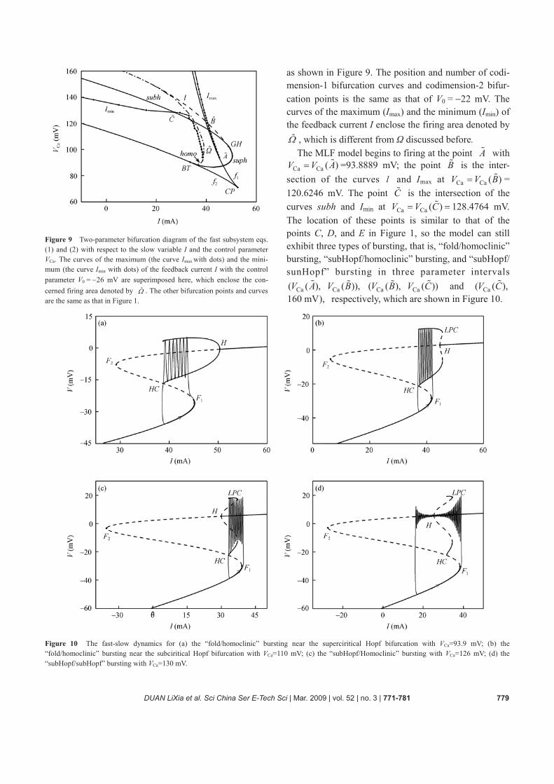
Figure 9 Two-parameter bifurcation diagram of the fast subsystem eqs. (1) and (2) with respect to the slow variable I and the control parameter VCa. The curves of the maximum (the curve Imax with dots) and the mini-mum (the curve Imin with dots) of the feedback current I with the control parameter V0 = −26 mV are superimposed here, which enclose the con-cerned firing area denoted by Ω . The other bifurcation points and curves are the same as that in Figure 1.

as shown in Figure 9. The position and number of codi-mension-1 bifurcation curves and codimension-2 bifur-cation points is the same as that of V0 = −22 mV. The curves of the maximum (Imax) and the minimum (Imin) of the feedback current I enclose the firing area denoted by Ω , which is different from Ω discussed before.

The MLF model begins to firing at the point A with Ca Ca ( )V V A= =93.8889 mV; the point B is the inter-

section of the curves l and Imax at Ca Ca ( )V V B= = 120.6246 mV. The point C is the intersection of the curves subh and Imin at Ca Ca ( )V V C= = 128.4764 mV. The location of these points is similar to that of the points C, D, and E in Figure 1, so the model can still exhibit three types of bursting, that is, “fold/homoclinic” bursting, “subHopf/homoclinic” bursting, and “subHopf/ sunHopf” bursting in three parameter intervals

Ca Ca( ( ), ( )),V A V B Ca Ca( ( ), ( ))V B V C and Ca( ( ),V C 160 mV), respectively, which are shown in Figure 10.

Figure 10 The fast-slow dynamics for (a) the “fold/homoclinic” bursting near the superciritical Hopf bifurcation with VCa=93.9 mV; (b) the “fold/homoclinic” bursting near the subciritical Hopf bifurcation with VCa=110 mV; (c) the “subHopf/Homoclinic” bursting with VCa=126 mV; (d) the “subHopf/subHopf” bursting with VCa=130 mV.


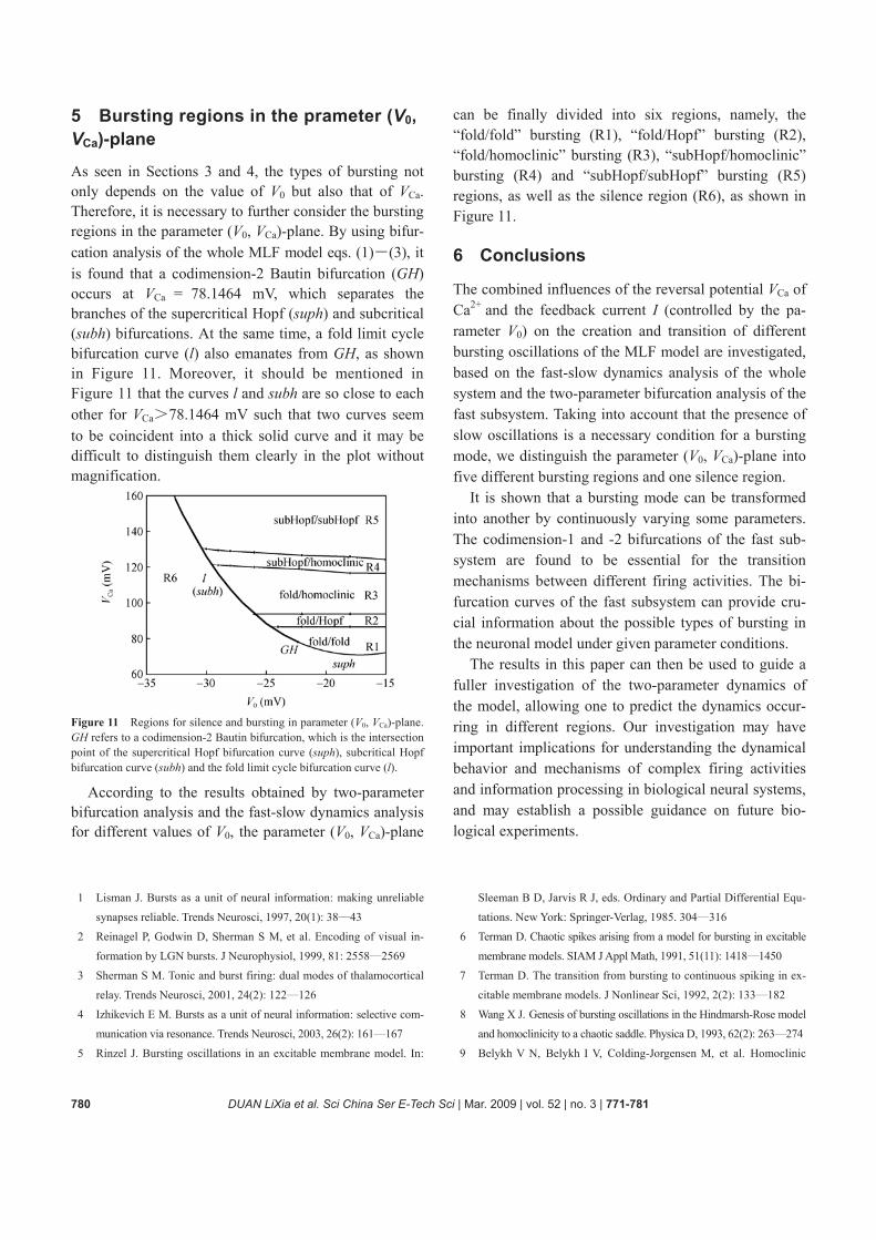
5 Bursting regions in the prameter (V0, VCa)-plane

As seen in Sections 3 and 4, the types of bursting not only depends on the value of V0 but also that of VCa. Therefore, it is necessary to further consider the bursting regions in the parameter (V0, VCa)-plane. By using bifur-cation analysis of the whole MLF model eqs. (1)―(3), it is found that a codimension-2 Bautin bifurcation (GH) occurs at VCa = 78.1464 mV, which separates the branches of the supercritical Hopf (suph) and subcritical (subh) bifurcations. At the same time, a fold limit cycle bifurcation curve (l) also emanates from GH, as shown in Figure 11. Moreover, it should be mentioned in Figure 11 that the curves l and subh are so close to each other for VCa＞78.1464 mV such that two curves seem to be coincident into a thick solid curve and it may be difficult to distinguish them clearly in the plot without magnification.

Figure 11 Regions for silence and bursting in parameter (V0, VCa)-plane. GH refers to a codimension-2 Bautin bifurcation, which is the intersection point of the supercritical Hopf bifurcation curve (suph), subcritical Hopf bifurcation curve (subh) and the fold limit cycle bifurcation curve (l).

According to the results obtained by two-parameter bifurcation analysis and the fast-slow dynamics analysis for different values of V0, the parameter (V0, VCa)-plane

can be finally divided into six regions, namely, the “fold/fold” bursting (R1), “fold/Hopf” bursting (R2), “fold/homoclinic” bursting (R3), “subHopf/homoclinic” bursting (R4) and “subHopf/subHopf” bursting (R5) regions, as well as the silence region (R6), as shown in Figure 11.

6 Conclusions

The combined influences of the reversal potential VCa of Ca2+ and the feedback current I (controlled by the pa-rameter V0) on the creation and transition of different bursting oscillations of the MLF model are investigated, based on the fast-slow dynamics analysis of the whole system and the two-parameter bifurcation analysis of the fast subsystem. Taking into account that the presence of slow oscillations is a necessary condition for a bursting mode, we distinguish the parameter (V0, VCa)-plane into five different bursting regions and one silence region.

It is shown that a bursting mode can be transformed into another by continuously varying some parameters. The codimension-1 and -2 bifurcations of the fast sub-system are found to be essential for the transition mechanisms between different firing activities. The bi-furcation curves of the fast subsystem can provide cru-cial information about the possible types of bursting in the neuronal model under given parameter conditions.

The results in this paper can then be used to guide a fuller investigation of the two-parameter dynamics of the model, allowing one to predict the dynamics occur-ring in different regions. Our investigation may have important implications for understanding the dynamical behavior and mechanisms of complex firing activities and information processing in biological neural systems, and may establish a possible guidance on future bio-logical experiments.

1 Lisman J. Bursts as a unit of neural information: making unreliable

synapses reliable. Trends Neurosci, 1997, 20(1): 38―43

2 Reinagel P, Godwin D, Sherman S M, et al. Encoding of visual in-

formation by LGN bursts. J Neurophysiol, 1999, 81: 2558―2569

3 Sherman S M. Tonic and burst firing: dual modes of thalamocortical

relay. Trends Neurosci, 2001, 24(2): 122―126

4 Izhikevich E M. Bursts as a unit of neural information: selective com-

munication via resonance. Trends Neurosci, 2003, 26(2): 161―167

5 Rinzel J. Bursting oscillations in an excitable membrane model. In:

Sleeman B D, Jarvis R J, eds. Ordinary and Partial Differential Equ-

tations. New York: Springer-Verlag, 1985. 304―316

6 Terman D. Chaotic spikes arising from a model for bursting in excitable

membrane models. SIAM J Appl Math, 1991, 51(11): 1418―1450

7 Terman D. The transition from bursting to continuous spiking in ex-

citable membrane models. J Nonlinear Sci, 1992, 2(2): 133―182

8 Wang X J. Genesis of bursting oscillations in the Hindmarsh-Rose model

and homoclinicity to a chaotic saddle. Physica D, 1993, 62(2): 263―274

9 Belykh V N, Belykh I V, Colding-Jorgensen M, et al. Homoclinic


bifurcations leading to the emergence of bursting oscillations in cell

models. Eur Phys J E, 2000, 3(2): 205―219

10 Guckenheimer J, Tien J H. Bifurcation in the fast dynamics of neu-

rons: implication for bursting. In: Coombes S, Bressloff P C, eds.

The Genesis of Rhythm in the Nervous System. Bursting: World

Scientific Publish, 2005. 89―122

11 Shorten P R, Wall D J. A Hodgkin-Huxley model exhibiting bursting

oscillations. Bull Math Biol, 2000, 62(6): 695―715

12 Bertram R, Butte M, Kiemel T, et al. Topological and phenomenol-

ogical classification of bursting oscillations. Bull Math Biol, 1995,

57(4): 413―439

13 Xie Y, Duan Y B, Xu J X, et al. Parabolic bursting induced by

veratridine in rat injured sciatic nerves. ACTA Bioch Bioph Sin, 2003,

35(9): 806―810

14 Yang Z Q, Lu Q S. Different types of bursting in Chay neuronal

model. Sci China Ser G-Phys Mech Astron, 2008, 51(6): 687―698

15 Channell P, Cymbalyuk G, Shilnikov A. Origin of bursting through

homoclinic spike adding in a neuron model. Phys Rev Lett, 2007,

98(13): 134101

16 Ibarz B, Cao H J, Sanjuán, M A F. Bursting regimes in map-based

neuron models coupled through fast threshold modulation. Phys Rev

E, 2008, 77(5-1): 051918

17 Shen Y, Hou Z H, Xin H W. Transition to burst synchronization in

coupled neuron networks. Phys Rev E, 2008, 77(3-1): 031920

18 Duan L X, Lu Q S, Wang Q Y. Two-parameter bifurcation analysis of

firing activities in the Chay neuronal model. Neurocomp, 2008.

doi:10.1016/j.neucom.2008.01.019

19 Morris C, Lecar H. Voltage oscillations in the barnacle giant muscle

fiber. Biophys J, 1981, 35(2): 193―213

20 Izhikevich E M. Neural excitability, spiking and bursting. Int J Bi-

furcat Chaos, 2000, 10(10): 1171―1266

21 Tsumoto K, Kitajima H. Bifurcation in Morris-Lecar neuron model.

Neurocomp, 2006, 69(2): 293―316

22 Hoppensteadt F C, Izhikevich E M. Weakly Connected Neural Net-

works. New York: Springer-Verlag, 1997

23 Ghigliazza R M, Holmes P. Minimal models of bursting neurons:

how multiple currents, conductances, and time scales affect bifurca-

tion diagrams. SIAM J Appl Dyn Syst, 2004, 3(4): 636―667

24 Ermentrout G B. Simulating, analyzing, and animating dynamical

systems: a guide to XPPAUT for researchers and students. Philadel-

phia: SIAM, 2002

25 Kuznetsov Y A. Elements of Applied Bifurcation Theory. New York:

Springer-Verlag, 1995. 253―265

26 Kuznetsov Y A, Levitin V V. Content-1.5-ibmpc-mswin-bcc55. zip.

http: //www. math. uu. nl/people/kuznet/CONTENT

27 Holden L, Erneux T. Slow passage through a Hopf bifurcation: Form

oscillatory to steady state solutions. SIAM J Appl Math, 1993 (53):

1045―1058

Documents

Bursting of Morris-Lecar neuronal model with current-feedback control