CALCULATING LIQUEFACTION POTENTIAL OF NORTHERN MISSISSIPPI

USING SHEAR WAVE DATA

by

Peshani Herath

A thesis submitted to the faculty of The University of Mississippi in partial fulfillment of

the requirements of the Sally McDonnell Barksdale Honors College.

Oxford

May 2016

Approved by

_________________________________

Advisor: Dr. Craig Hickey

_________________________________

Reader: Dr. Zhen Guo

_________________________________

Reader: Dr. Christopher Mullen

ii

© 2016

Peshani Herath

ALL RIGHTS RESERVED

iii

ACKNOWLEDGEMENTS

Thank you to Dr. Craig Hickey, without whom this study would not be possible,

for his guidance and patience. The support of Leti Wodajo in analyzing and collecting

data is much appreciated. The work done by Dakota Kolb and Blake Armstrong in

collecting shear wave data is extremely valued. Thank you to Ina Aranchuk, Dr. Zhen

Guo, Kristin Davidson, Dr. Louis Zachos, and Christian Kunhardt for their invaluable

help in MatLab and/or ArcGIS. Thank you to Dr. Christopher Mullen for correcting and

giving valuable feedback on my paper. Finally thank you to the National Center for

Physical Acoustics for providing the equipment for this project and the Sally McDonnell

Barksdale Honors College for encouraging me to participate in research.

iv

ABSTRACT

PESHANI HERATH: Calculating Liquefaction Potential of Northern Mississippi Using

Shear Wave Data

(Under the direction of Dr. Craig Hickey)

The potential for liquefaction can be determined using the Liquefaction Potential

Index (LPI). The LPI takes into account the thickness of the liquefiable layers and the

factors of safety with respect to depth. This study creates a hybrid method for

determining the LPI for different locations in Northern Mississippi. It calculates an

average CSR for the region using existing borehole information. The CRR is then

calculated using shear wave velocity profile data from a MASW survey. The LPI

obtained from this process is compared to LPI values calculated using CPT data and

borehole shear wave data. Surface shear wave velocity profiles are measured near two

existing borehole locations, TNA013 and TNA012. The sites near borehole TNA013 and

TNA012 are both very highly liquefiable according to the MASW method, but are only

highly liquefiable using the borehole shear wave method. The LPI value calculated using

CPT data near borehole TNA013 is classified as highly liquefiable and the LPI value near

borehole TNA012 is classified as having a low liquefaction potential. The hybrid method

gives a more conservative estimate of the liquefaction potential in the study area than the

CPT method or borehole shear wave data.

v

TABLE OF CONTENTS

LIST OF TABLES.............................................................................................................. vi

LIST OF FIGURES........................................................................................................... vii

CHAPTER 1: INTRODUCTION........................................................................................ 1

CHAPTER 2: LIQUEFACTION......................................................................................... 7

2.1: CALCULATING LIQUEFACTION POTENTIAL............................... 14

2.1.1: DETERMINING FACTOR OF SAFETY USING.............................. 19

THE STANDARD PENETRATION TEST (SPT)

2.1.2: DETERMINING FACTOR OF SAFETY USING.............................. 20

CONE PENETRATION TEST (CPT)

2.1.3: DETERMINING FACTOR OF SAFETY USING.............................. 23

SHEAR WAVE VELOCITY

CHAPTER 3: NORTHERN MISSISSIPPIDELTA DATA............................................. 25

3.1: REPRODUCTION OF RESULTS BY SONG AND MIKELL............. 30

3.2: CALCULATING LPI USING AVERAGE CSR................................... 34

3.2.1: CALCULATING AVERAGE CSR..................................................... 34

3.3: CALCULATING RESULTS BY SONG AND MIKELL...................... 36

USING SHEAR WAVE DATA

3.4: LIQUEFACTION POTENTIAL AND VS30 DATA............................. 41

FROM SHEAR WAVEVELOCITY DATA

CHAPTER 4: CALCULATING LIQUEFACTION USING SURFACE......................... 42

SHEAR WAVE METHOD

CHAPTER 5: CONCLUSION..........................................................................................50

BIBILIOGRAPHY............................................................................................................51

vi

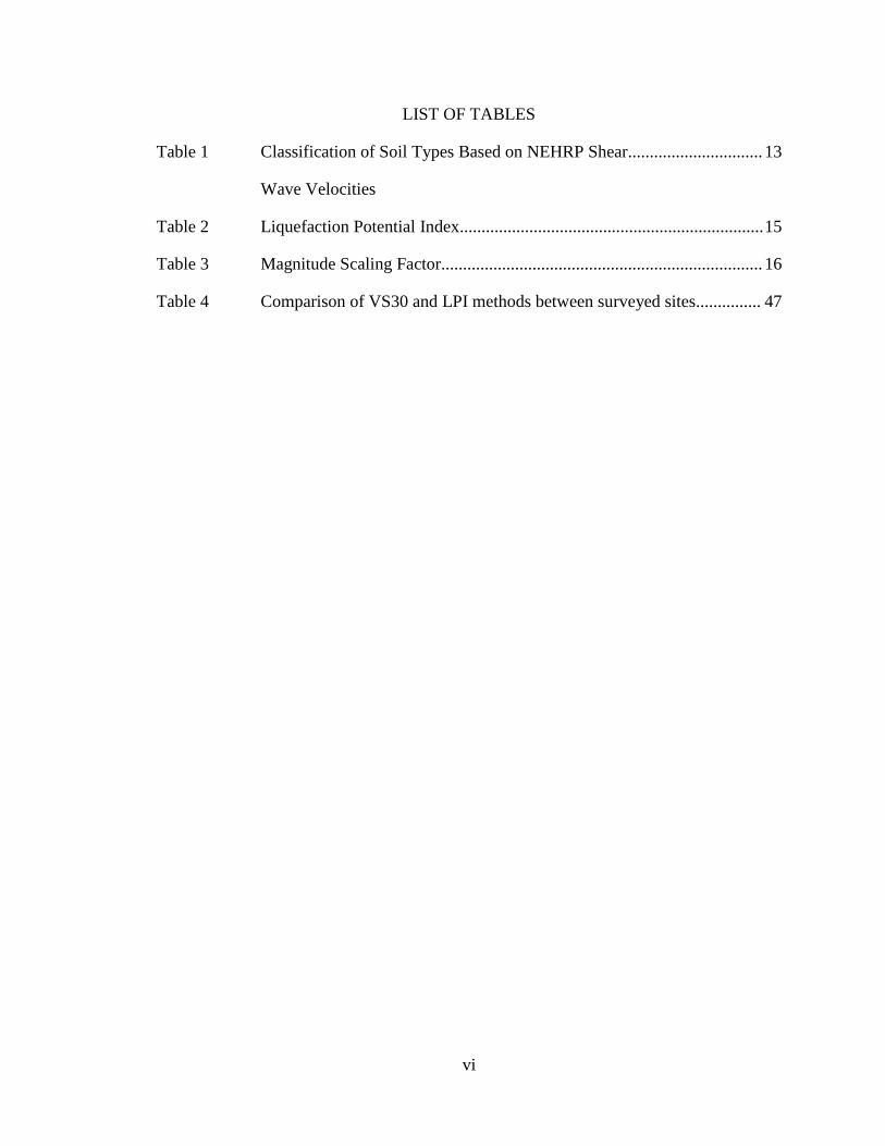
LIST OF TABLES

Table 1 Classification of Soil Types Based on NEHRP Shear............................... 13

Wave Velocities

Table 2 Liquefaction Potential Index...................................................................... 15

Table 3 Magnitude Scaling Factor.......................................................................... 16

Table 4 Comparison of VS30 and LPI methods between surveyed sites............... 47

vii

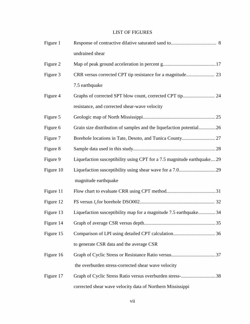
LIST OF FIGURES

Figure 1 Response of contractive dilative saturated sand to..................................... 8

undrained shear

Figure 2 Map of peak ground acceleration in percent g........................................... 17

Figure 3 CRR versus corrected CPT tip resistance for a magnitude....................... 23

7.5 earthquake

Figure 4 Graphs of corrected SPT blow count, corrected CPT tip.......................... 24

resistance, and corrected shear-wave velocity

Figure 5 Geologic map of North Mississippi........................................................... 25

Figure 6 Grain size distribution of samples and the liquefaction potential.............. 26

Figure 7 Borehole locations in Tate, Desoto, and Tunica County........................... 27

Figure 8 Sample data used in this study................................................................... 28

Figure 9 Liquefaction susceptibility using CPT for a 7.5 magnitude earthquake.... 29

Figure 10 Liquefaction susceptibility using shear wave for a 7.0.............................. 29

magnitude earthquake

Figure 11 Flow chart to evaluate CRR using CPT method........................................ 31

Figure 12 FS versus 𝐼𝑐for borehole DSO002............................................................. 32

Figure 13 Liquefaction susceptibility map for a magnitude 7.5 earthquake.............. 34

Figure 14 Graph of average CSR versus depth.......................................................... 35

Figure 15 Comparison of LPI using detailed CPT calculation.................................. 36

to generate CSR data and the average CSR

Figure 16 Graph of Cyclic Stress or Resistance Ratio versus.................................... 37

the overburden stress-corrected shear wave velocity

Figure 17 Graph of Cyclic Stress Ratio versus overburden stress-............................ 38

corrected shear wave velocity data of Northern Mississippi

viii

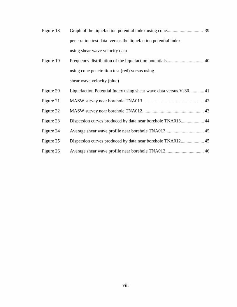
Figure 18 Graph of the liquefaction potential index using cone............................... 39

penetration test data versus the liquefaction potential index

using shear wave velocity data

Figure 19 Frequency distribution of the liquefaction potentials............................... 40

using cone penetration test (red) versus using

shear wave velocity (blue)

Figure 20 Liquefaction Potential Index using shear wave data versus Vs30............. 41

Figure 21 MASW survey near borehole TNA013..................................................... 42

Figure 22 MASW survey near borehole TNA012..................................................... 43

Figure 23 Dispersion curves produced by data near borehole TNA013.................... 44

Figure 24 Average shear wave profile near borehole TNA013................................. 45

Figure 25 Dispersion curves produced by data near borehole TNA012.................... 45

Figure 26 Average shear wave profile near borehole TNA012................................. 46

1

1.0 Introduction

The Earth’s crust is continuously moving atop a plastic layer called the

asthenosphere. When this motion is hindered, strain can form in the lithosphere. This

strain energy is released and manifests itself as an earthquake (Spall, 1977). Seismic

activity can occur along plate boundaries (interplate) or in the interior of a tectonic plate

(intraplate) (Lowrie, 1997). The majority of earthquakes originate from interplate seismic

activity (Lowrie, 1997).

The seismic zones associated with interplate tectonics can be divided into those

that follow mid-ocean ridges, continental plate boundaries, ocean-continent boundaries,

and those caused by plates sliding by each other (Spall, 1977).

The processes that create intraplate earthquakes are more complex than those

produced by plate boundaries and cannot be explained well through plate tectonics

(Fillingim, 1999). One explanation for the existence of intraplate seismic activity is the

zones of weakness in the Earth’s crust. Weaknesses can arise from previous tectonic

activities like failed ancient rift zones and passive margins deformed due to the

development of active spreading centers. Over time, these zones can become

incorporated into the central portion of a plate and remain inactive for many years. In the

presence of stresses, these zones can get reactivated.

According to the United States Geological Survey, compared to the rest of the

state Mississippi, the northern portion is the most at risk from an earthquake. This is due

to the intraplate activity caused by the New Madrid Fault Zone (United States Geological

2

Survey, 2012). The New Madrid Seismic Zone is a compilation of several thrust faults

that stretch from Arkansas to Illinois (Central United States Earthquake Consortium,

2016). It is the most active seismic area in the United States east of the Rocky Mountains

(Missouri Department of Natural Resources, 2014). The New Madrid Seismic Zone

encompasses northeastern Arkansas, southeastern Missouri, western Missouri, western

Tennessee, southern Illinois, western Kentucky, southwestern Indiana, and northwestern

Mississippi.

An ancient failed rift called the Reelfoot Rift underlies the Mississippi

Embayment with a thick section of sedimentary rock filling the graben, or fault blocks

located between two major faults, associated with the rift. The New Madrid Seismic Zone

is located at the center of the buried rift (Braile et al., 1986). The correlation of the

earthquake epicenters with the buried rift complex indicates that the earthquakes in the

New Madrid Seismic Zone are results of slippage along pre-existing zones of weakness.

Contemporary stress fields going east to west in the New Madrid area reactivate these

fault planes (Braile et al., 1986).

Due to the harder, colder, drier and less fractured nature of the rocks, earthquakes

in the central or eastern United States have a larger impact than earthquakes with similar

magnitude in the western United States. They shake and damage a region 20 times larger

than earthquakes in California (Missouri Department of Natural Resources, 2014). The

effects of the New Madrid earthquake on December 1811 could be felt thousands of

miles from the epicenter (United States Geological Survey, 2012). Three very large

earthquakes occurred in 1811 – 1812 that are referred to as New Madrid earthquakes after

a town in Missouri. The first principle earthquake that occurred in northeast Arkansas

3

December 16, 1811 was a magnitude 7.7. This was followed by a second primary shock

in Missouri on January 23, 1812 with a magnitude of 7.5. The third principle shock was a

magnitude 7.7 that occurred on February 7, 1812 along the Reelfoot fault in Missouri and

Tennessee. Four aftershocks, each ranging in magnitude from 6.0 to 6.5 also occurred

during this period. A report by Otto Nuttli states that more than 200 moderate to large

aftershocks occurred in the New Madrid region between December 16, 1811 and March

15, 1812 (United States Geological Survey, 2012).

The primary cause of destruction in modern earthquakes is the collapse of

manmade structures (Missouri Department of Natural Resources, 2014).In addition to the

shaking from surface waves, damage to structures can occur when the foundation

liquefies. Liquefaction is the tendency of an unconsolidated saturated soil to behave like a

liquid when introduced to a shock, commonly an earthquake (Rauch, 1997). Liquefaction

potential is related to the amount of subsurface ground water and its proximity to the

surface, the soil type, and the magnitude and of the seismic activity at a given location.

Liquefaction of soils is largely dependent on the Cyclic Stress Ratio (CSR), the measure

of earthquake loading, and Cyclic Resistance Ratio (CRR), liquefaction resistance of the

ground (University of Washington, 2016).

Liquefaction resistance of soils can be evaluated using several methods. The

earliest and simplest method is based on the Standard Penetration Test (SPT). Later

methods included the Cone Penetration Test (CPT), and small strain shear wave velocity

(Vs) measurements (Andruset al., 2003). Because of the poor repeatability and inherent

difficulties associated with the Standard Penetration Test, the CPT is used as a method to

determining CRR for clean and silty sands (Robertson and Wride, 1998).

4

The Cone Penetration Test (CPT) can be useful in characterizing sites with

discrete stratigraphic horizons or discontinuous lenses. It is valuable in accessing

subsurface stratigraphy associated with soft material, discontinuous lenses, potentially

liquefiable material, and landslides. In this method, a 1.41 inch diameter 55° to 60° cone

is pushed through the underlying ground at a rate of 1 to 2 centimeters per second

(Rodgers, 2004). A computerized log of the tip and sleeve resistance, induced pore

pressure behind the cone tip, pore pressure ratio, and a lithologic interpretation of every

two centimeter interval are produced. The tip resistance of a cone is related to the

undrained shear strength of a saturated cohesive material while the sleeve friction is

related to the friction of the horizon being penetrated. The higher the tip resistance, the

less likely liquefaction will occur (Robertson and Wride, 1998).

Seismic waves can also be measured during a CPT. As a borehole is created using

this technique a cone with seismic capabilities, seismic cone, can detect shear waves

(Song and Mikell, 2013). The borehole shear wave velocity is an alternative method to

determine liquefaction. Unlike the penetration tests, this measurement is better in

gravelly soils and capped landfills (Andrus et al., 2003). In addition to use in liquefaction

studies, multiple studies have established that shear-waves in the upper 30 to 60 meters

can greatly affect surface ground motion duration and amplification of an earthquake.

The average shear wave velocity in the top 30 m, known as Vs30, is the metric obtained

from the shear wave velocity profile to correlate with amplification (Odum, 2007).

A shear wave velocity profile can also be measured using surface refraction and

multichannel analysis of surface waves, MASW, methods. Multichannel analysis of

surface waves is becoming more popular in geotechnical studies and measures the speed

5

of the surface waves. The seismic waves are produced by impacting the ground with a

sledgehammer. This energy is detected by a multiple channel recording system and a

receiver array that is spread out over hundreds of meters. A dispersion curve (surface

wave velocity versus frequency) is then calculated from this data and inverted to obtain a

shear wave versus depth profile (Park, 2007).

The potential for liquefaction can be determined using the Liquefaction Potential

Index (LPI). The LPI takes into account the thickness of the liquefiable layers and the

factors of safety with respect to depth. The purpose of this study is to create a hybrid

method for determining the LPI for different locations in Northern Mississippi. The

hybrid method uses an average CSR for the region calculated using existing borehole

information. The local CRR is calculated using a shear wave velocity profile obtained

from a MASW survey. This hybrid method would not require additional CPT or

boreholes. In order to evaluate the feasibility of this hybrid method, the LPI is calculated

using CPT following the method of Song and Mikell (2013). Then, an average CSR is

calculated using all the borehole data in the region and the LPI is recalculated using the

average CSR. The viability between the two LPI values is less than ten percent. The LPI

is then calculated using shear wave velocity from boreholes and compared to the CPT

derived LPI. There was no discernable pattern between the two calculations. The LPI

values calculated using the borehole shear wave method are generally higher (more

liquefiable) than the LPI values using CPT data. The LPI using shear wave velocity and

Vs30 measured at the various boreholes are also compared. These values correlated with

low velocities indicating high liquefaction potentials. Surface shear wave velocity

profiles are measure at two borehole locations using the MASW survey method. These

6

two shear wave profiles are used to calculate a LPI value using the average CSR as well

as the Vs30 value. The site near borehole TNA013 is very highly liquefiable according

to the MASW method and highly liquefiable using the borehole shear wave method. It

has a soil type of D according to Vs30 values. The site near borehole TNA012 is very

highly liquefiable using MASW data and highly liquefiable using borehole shear wave

data. It is classified as soil type E according to the Vs30 values.

7

2.0 Liquefaction

In general, liquefaction is used to refer to all the failure mechanisms due to pore

pressure build-up during cyclic shear of undrained, saturated soil. When subjected to

shearing stresses, loose saturated soil grains tend to be rearranged into to a denser

packing. When this occurs, there is less space and the water in the pore space is forced

out. However, the pore pressure will increase as the shear load increases if the drainage

of the pore water is obstructed. This transfers the stress from the soil skeleton to the pore

water, and can lead to the reduction of effective stress and shear resistance of the soil.

When the shear resisting stress is less than the driving shear stress, the soil undergoes

deformation, or liquefaction (Rauch, 1997).

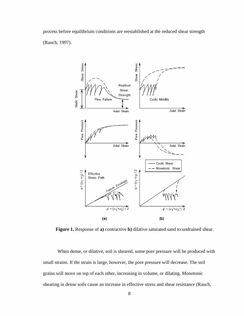
When loose, or contractive soil, is sheared monotonically, it reaches peak shear

strength and softens to a residual shear resistance (top Figure 1a). Liquefaction flow

failure occurs when the static driving stress exceeds the residual shear resistance (Rauch,

1997).When this same soil is sheared cyclically, excess pore pressure is generated with

each load cycle (middle Figure 1a). Without pore water drainage, the pore pressure

increases causing the system to move towards failure. If the static driving stress is greater

than the shear strength, flow failure occurs and continues even after the cyclic load is

removed. In order for liquefaction to occur where the shear resistance is overcome by the

static driving load, a contracting saturated soil must undergo sufficient undrained stress

for an adequate number of load cycles. A great amount of damage can be caused with this

8

process before equilibrium conditions are reestablished at the reduced shear strength

(Rauch, 1997).

Figure 1. Response of a) contractive b) dilative saturated sand to undrained shear.

When dense, or dilative, soil is sheared, some pore pressure will be produced with

small strains. If the strain is large, however, the pore pressure will decrease. The soil

grains will move on top of each other, increasing in volume, or dilating. Monotonic

shearing in dense soils cause an increase in effective stress and shear resistance (Rauch,

9

1997). When the same soil is dynamically loaded, each load cycle will generate some

pore pressure, resulting in deformation (middle Figure 1b). At a certain point, however,

further strain is prevented by the tendency of the soil to increase in volume. Flow failure

does not occur in undrained dilative soil during cyclic loading because the shear strength

remains greater than the static diving shear stress. This behavior is called cyclic mobility

(Rauch, 1997).

P. K. Robertson and C. E. Fear in 1996 suggested a classification system to define

soil liquefaction. The two major categories are flow liquefaction and cyclic softening.

Flow liquefaction is used for saturated, undrained flow of a contractive, or loose, soil

when static residual stress exceeds the residual shear strength of the soil (Rauch, 1997).

Cyclic softening is used for undrained dilating soils that experience large deformation

during cyclic shearing due to pore pressure build up. This category can be further divided

into cyclic liquefaction and cyclic mobility. Cyclic liquefaction describes the condition

when cyclic shear stresses are greater than the initial static shear stress, creating a stress

reversal. This can produce a stress reversal where a condition of zero effective stress can

be present during which large deformation can occur (Rauch, 1997). Cyclic mobility is

where deformation is accumulated in each cycle of shear stress where conditions of zero

effective stress do not develop (Rauch, 1997).

Loose, saturated, shallow deposits of cohesionless soils that produce strong

ground motion during large magnitude earthquakes are most susceptible to liquefaction

(Rauch, 1997). Liquefaction and large deformation are more common with soils that are

compressive as opposed to dilative that tend to experience cyclic softening and limited

10

deformation. Unsaturated soils do not experience liquefaction because pore pressure is

not generated when the soil volume is decreased (Rauch, 1997).

Liquefaction causes soil grains to rearrange themselves. Anything that hinders

this motion will increase the resistance of a soil to liquefaction. Factors related to the

geologic formation of the deposit like particle cementation, soil fabric, and aging can

hinder the process of rearranging grains (Rauch, 1997). The stress history of a soil can

also affect the liquefaction potential. Deposits with uneven consolidation conditions, for

example, are more resistant to pore pressure generation. Soils that have been over-

consolidated are less likely to experience liquefaction because they have been exposed to

greater static pressure, reducing the likelihood of the grains rearranging themselves

(Rauch, 1997). Soils buried deeper than approximately 15 meters are more resistant to

liquefaction because the effective overburden pressure increases with depth. This is

because the frictional resistance between the grains is proportional to the effective

confining stress (Rauch, 1997).

The characteristics of the soil grains such as shape, size distribution, and

composition also influence the liquefaction susceptibility. Generally, sands and silt are

most susceptible to liquefaction, but there are records of gravel liquefying. Well graded,

angular sand particles are less likely to experience liquefaction because the interlocking

of the grains is more stable. Silty sand, however, are prone to liquefaction because they

are deposited loosely. Rounded grains with uniform size distribution are most susceptible

to liquefaction (Rauch, 1997).

Clays with measureable plasticity can hinder the movement of grains during

cyclic shearing. This impedes the generation of pore pressure, reducing liquefaction.

11

Liquefaction is rarely observed in soils with a large quantity of plastic fines because the

adhesion created between the grains impedes the larger particles from moving into a

denser arrangement. Non-plastic fines, however, contribute to liquefaction because they

are inherently collapsible and inhibit the drainage of excess pore pressure (Rauch, 1997).

The permeability of the soil is another parameter controlling liquefaction. Soils

that are less permeable cannot transport pore fluids and cause pore pressure to build up

during cyclic loading. The permeability of the surrounding rock will also influence

liquefaction susceptibility. Permeable layers above and below a saturated soil can help

dissipate the excess pore water, decreasing pore pressure. This high permeability is why

gravelly soils are less prone to liquefaction (Rauch, 1997).

Liquefaction does not occur in places at random; rather, they are controlled by a

certain geologic and hydrologic environment (Greene and Youd, 1994). Relatively

younger, looser soils deposited in an area with high ground water levels provides the

optimum conditions for liquefaction. Areas with the ground water table within ten meters

of the ground surface tend to be areas with the most abundant occurrences of liquefaction

(Greene and Youd, 1994). The opportunity of liquefaction occurring is restricted by the

frequency of earthquake occurrence and the intensity of seismic ground shaking. Seismic

source zones must be taken into account if a liquefaction opportunity map is to be

developed. Seismic motion is more intense the closer the site is to the source of the

disturbance, and will increase the opportunity for liquefaction (Greene and Youd, 1994).

Even if the soil has the necessary characteristics for liquefaction to occur, it will

not occur until the proper stress or ground motion from earthquakes is present. The

primary factors controlling how the surface soil behaves in the presence of an earthquake

12

are shear wave velocity, depth to hard rock, and non-linear dynamic material properties

(Silva, 2003).

Multiple studies (Borcherdt and Gibbs, 1976; Joyner et al., 1981; Seed et al.,

1988) have established that shear-waves in the upper 30 to 60 meters can greatly affect

surface ground motion duration and amplification of an earthquake. Shallow Vs is

referred to as Vs30 (Odum, 2007). The average Vs is calculated using velocity versus

depth profile to a depth of 30 meters (Odum, 2007) using the equation,

𝑉𝑆30 = ∑ 𝑑𝑖

𝑛𝑖=1

∑𝑑𝑖

𝑉𝑠𝑖

𝑛𝑖=1

(1)

where Vsi is the velocity of the ith layer and di is the thickness of the ith layer between 0 to

30 meters (Odum, 2007).

The velocity at which the soils transmit shear waves can contribute to the

amplification of motion. Ground shaking is stronger when the shear wave velocity is

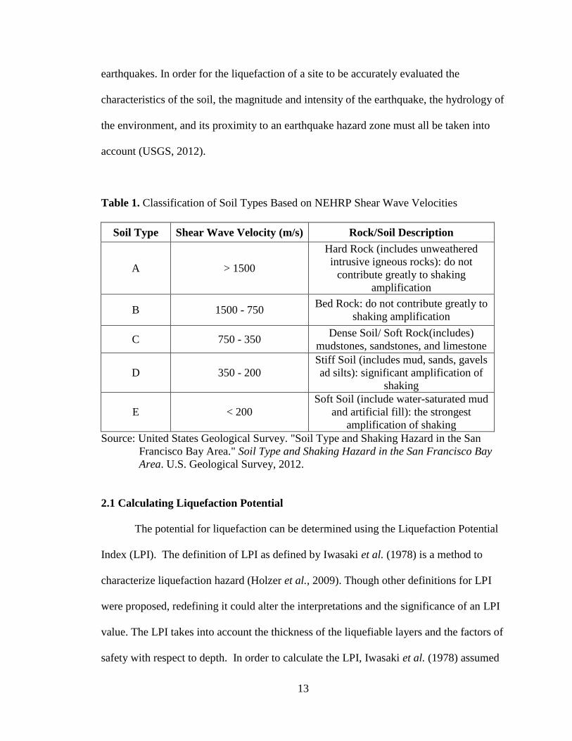
lower. Table 1 shows the five soil types defined by the National Earthquake Hazards

Reduction Program based on their shear wave velocities (USGS, 2012). High

amplification can lead to liquefaction. Therefore, soils that have high amplification may

also be susceptible to liquefaction.

The chart organizes soils ranging from least amount of amplification to the

greatest amount of amplification. Soil type E will experience the strongest ground motion

and soil type A will contribute least to ground motion amplification. S-waves travel faster

in hard rock than in soft soil (Odum, 2007). Soft soils amplify shear waves, so the ground

shaking in these areas are enhanced. Thin layers of soft soils that overlay stiffer soils or

bed rock, however, will behave as if the site were lying on stiff soil. Areas that have

endured earthquakes before will also experience greater ground motion during future

13

earthquakes. In order for the liquefaction of a site to be accurately evaluated the

characteristics of the soil, the magnitude and intensity of the earthquake, the hydrology of

the environment, and its proximity to an earthquake hazard zone must all be taken into

account (USGS, 2012).

Table 1. Classification of Soil Types Based on NEHRP Shear Wave Velocities

Soil Type Shear Wave Velocity (m/s) Rock/Soil Description

A > 1500

Hard Rock (includes unweathered

intrusive igneous rocks): do not

contribute greatly to shaking

amplification

B 1500 - 750 Bed Rock: do not contribute greatly to

shaking amplification

C 750 - 350 Dense Soil/ Soft Rock(includes)

mudstones, sandstones, and limestone

D 350 - 200

Stiff Soil (includes mud, sands, gavels

ad silts): significant amplification of

shaking

E < 200

Soft Soil (include water-saturated mud

and artificial fill): the strongest

amplification of shaking

Source: United States Geological Survey. "Soil Type and Shaking Hazard in the San

Francisco Bay Area." Soil Type and Shaking Hazard in the San Francisco Bay

Area. U.S. Geological Survey, 2012.

2.1 Calculating Liquefaction Potential

The potential for liquefaction can be determined using the Liquefaction Potential

Index (LPI). The definition of LPI as defined by Iwasaki et al. (1978) is a method to

characterize liquefaction hazard (Holzer et al., 2009). Though other definitions for LPI

were proposed, redefining it could alter the interpretations and the significance of an LPI

value. The LPI takes into account the thickness of the liquefiable layers and the factors of

safety with respect to depth. In order to calculate the LPI, Iwasaki et al. (1978) assumed

14

that the severity of liquefaction is related to the total thickness of the liquefied layers, the

depth of these layers (proximity to the surface), and how much less the liquefaction factor

of safety (FS) is to one. The FS is a measure of the soil's capacity to resist liquefaction

during an earthquake (Holzer et al., 2009). The LPI is defined as,

𝐿𝑃𝐼 = ∫ 𝐹𝐿 × 𝑤(𝑧)𝑑𝑧20

0 (2)

𝑤(𝑧) = 10 − 0.5𝑧 (3)

𝐹𝐿 = 1 − 𝐹𝑆 𝑓𝑜𝑟 𝐹𝑆 ≤ 1 (4)

𝐹𝐿 = 0 𝑓𝑜𝑟 𝐹𝑆 > 1 (5)

where 𝑧 is the depth in meters and 𝑤(𝑧) is a weighting factor that can vary from ten at

the surface to zero at 20 meters. Theoretically the value of the LPI can range from zero to

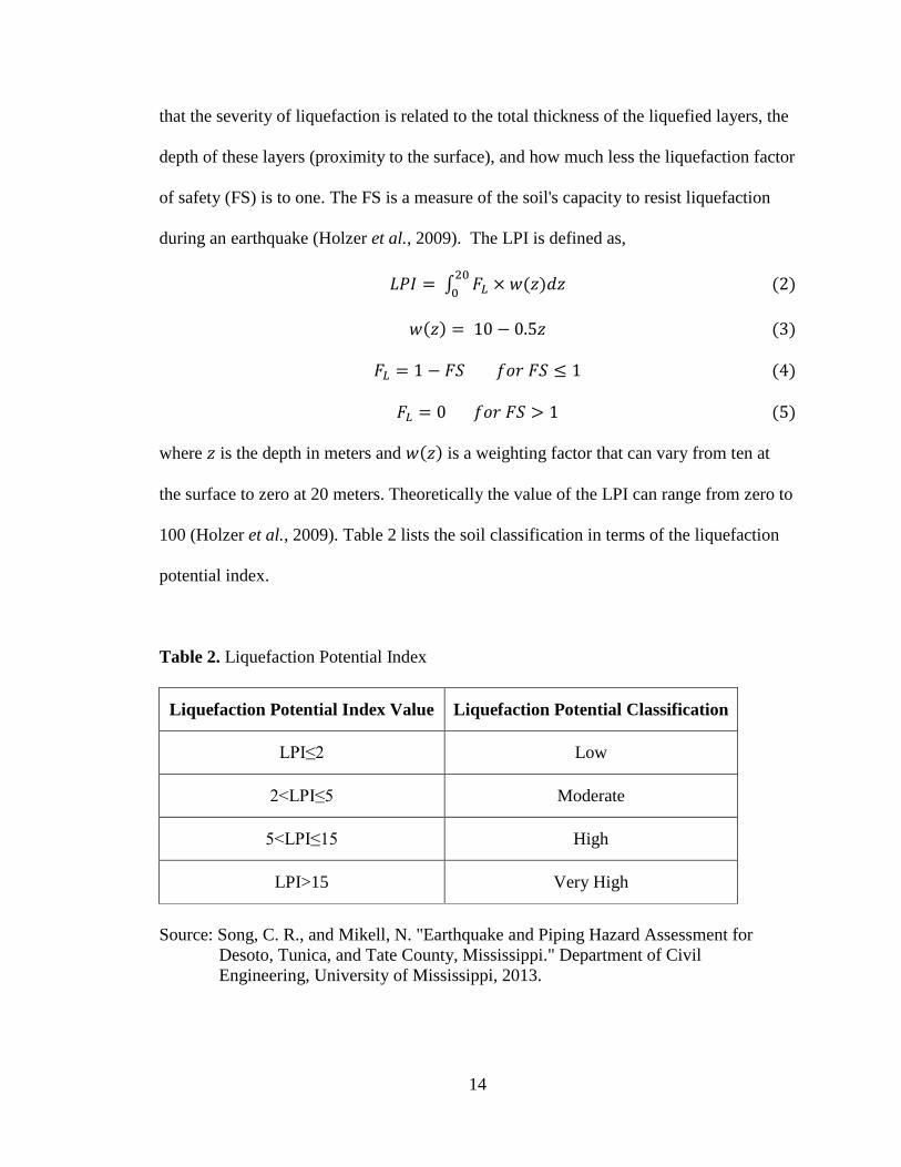
100 (Holzer et al., 2009). Table 2 lists the soil classification in terms of the liquefaction

potential index.

Table 2. Liquefaction Potential Index

Liquefaction Potential Index Value Liquefaction Potential Classification

LPI≤2 Low

2<LPI≤5 Moderate

5<LPI≤15 High

LPI>15 Very High

Source: Song, C. R., and Mikell, N. "Earthquake and Piping Hazard Assessment for

Desoto, Tunica, and Tate County, Mississippi." Department of Civil

Engineering, University of Mississippi, 2013.

15

The liquefaction potential is quantified using the Cyclic Resistance Ratio (CRR) and

Cyclic Stress Ratio (CSR). CRR represents dimensionless cyclic strength and CSR

represents dimensionless cyclic stress induced by an earthquake. The likelihood of

liquefaction occurring in terms of Cyclic Resistance Ratio for different ground layers is

determined using the Factor of Safety equation (Song and Mikell, 2013),

FS = CRR

CSR(MSF) (6)

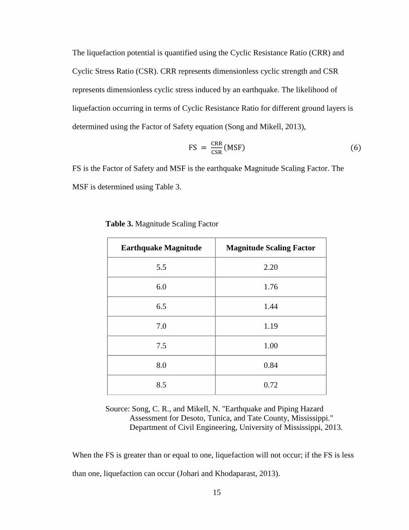
FS is the Factor of Safety and MSF is the earthquake Magnitude Scaling Factor. The

MSF is determined using Table 3.

Table 3. Magnitude Scaling Factor

Earthquake Magnitude Magnitude Scaling Factor

5.5 2.20

6.0 1.76

6.5 1.44

7.0 1.19

7.5 1.00

8.0 0.84

8.5 0.72

Source: Song, C. R., and Mikell, N. "Earthquake and Piping Hazard

Assessment for Desoto, Tunica, and Tate County, Mississippi."

Department of Civil Engineering, University of Mississippi, 2013.

When the FS is greater than or equal to one, liquefaction will not occur; if the FS is less

than one, liquefaction can occur (Johari and Khodaparast, 2013).

16

Liquefaction resistance of soils can be evaluated using the Standard Penetration

Test (SPT), the Cone Penetration Test (CPT), and small strain shear wave velocity (Vs)

measurements (Andrus et al., 2003). Each method has its advantages and disadvantages.

The calculation of CSR, however, is the same for all three methods.

The Cyclic Stress Ratio (CSR) is calculated using the equation,

𝐶𝑆𝑅 = 0.65𝑎𝑚𝑎𝑥

𝑔

𝜎𝑣0

𝜎𝑣0 ′ 𝑟𝑑 (7)

where 𝑎𝑚𝑎𝑥is the peak ground acceleration in percent g (g = 9.81 m/s), 𝜎𝑣0′ is the

effective vertical stress, 𝜎𝑣0is the total vertical stress, and 𝑟𝑑stress reduction factor. The

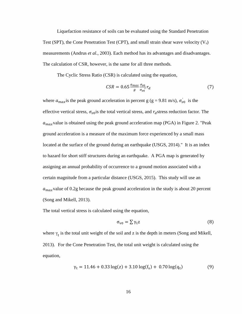
𝑎𝑚𝑎𝑥value is obtained using the peak ground acceleration map (PGA) in Figure 2. "Peak

ground acceleration is a measure of the maximum force experienced by a small mass

located at the surface of the ground during an earthquake (USGS, 2014)." It is an index

to hazard for short stiff structures during an earthquake. A PGA map is generated by

assigning an annual probability of occurrence to a ground motion associated with a

certain magnitude from a particular distance (USGS, 2015). This study will use an

𝑎𝑚𝑎𝑥value of 0.2g because the peak ground acceleration in the study is about 20 percent

(Song and Mikell, 2013).

The total vertical stress is calculated using the equation,

σv0 = ∑ γtz (8)

where γt is the total unit weight of the soil and z is the depth in meters (Song and Mikell,

2013). For the Cone Penetration Test, the total unit weight is calculated using the

equation,

γt = 11.46 + 0.33 log(𝑧) + 3.10 log(fs) + 0.70 log(qt) (9)

17

where z is the depth in meters, 𝑞𝑡 (kPA) is the tip resistance corrected for pore water

pressure, and fs (kPA) is the local friction measured from the CPT (Song and Mikell,

2013). The corrected tip resistance is calculated using,

𝑞𝑡 = 𝑞𝑐 + 𝑢2(1 − 𝑎𝑛) (10)

where 𝑞𝑐is the tip resistance measured during the CPT, u2 is the pore pressure measured

behind the cone, and 𝑎𝑛is the net area ratio. Typically, the 𝑎𝑛 value is between 0.7 and

0.8. In sands, 𝑞𝑐 can be used in equation 10 instead of 𝑞𝑡. This study will be using 𝑞𝑐

because the pore pressure behind the cone is unknown (Song and Mikell, 2013).

Figure 2. Map of peak ground acceleration in percent g (Song and Mikell, 2013).

The effective stress is calculated using the equation,

𝜎𝑣𝑜′ = 𝜎𝑣0 − 𝑝 (11)

where 𝑝 is the pore water pressure calculated using the equation,

𝑝 = γ(𝑧 − 𝑧0) (12)

18

where 𝑧 is the depth in meters, 𝑧0is the depth of the water table, and γ is the unit weight

of water (9.81 kN/m3). This study assumes the water table to be at one meter below the

surface (Song and Mikell, 2013).

The stress reduction factor is evaluated using the following guide lines,

𝑖𝑓𝑧 ≤ 9.15𝑚𝑒𝑡𝑒𝑟𝑠 𝑟𝑑 = 1.0 − 0.00765𝑧 (13)

𝑖𝑓 9.15 < 𝑧 ≤ 23𝑚𝑒𝑡𝑒𝑟𝑠 𝑟𝑑 = 1.174 − 0.0267𝑧 (14)

𝑖𝑓 23 < 𝑧 ≤ 30𝑚𝑒𝑡𝑒𝑟𝑠 𝑟𝑑 = 0.744 − 0.008𝑧 (15)

𝑖𝑓𝑧 > 30𝑚𝑒𝑡𝑒𝑟𝑠 𝑟𝑑 = 0.5 (16)

where 𝑧 is the depth in meters (Song and Mikell, 2013).

2.1.1 Determining Factor of Safety Using the Standard Penetration Test (SPT)

In the SPT method, blows from a slide hammer are used to drive a standard

thick-walled sample tube into the ground at the bottom of a deep narrow hole, borehole;

the slide hammer has standard weights and fall distance. The sample tube is driven up to

18 inches into the ground and the number of blows needed to penetrate every six inches is

recorded (geotechdata.info, 2013). The SPT blow count value is the sum of the number of

blows needed for the second and third six inches of penetration; it is also called the

standard penetration resistance and the N-value. This value indicates the relative density

of the subsurface soil and can be used to estimate the approximate shear strength

properties of the soil (geotechdata.info, 2013).

The CRR for an earthquake with a 7.5 magnitude is obtained using SPT results

by,

𝐶𝑅𝑅7.5 = 1

34−𝑁1,60𝑐𝑠+

𝑁1,60𝑐𝑠

135+

50

(10𝑁1,60𝑐𝑠+45)2−

1

200 (17)

19

𝑁1,60𝑐𝑠 is the clean sand equivalent of the overburden stress corrected SPT blow count,

𝑁1,60𝑐𝑠 = 𝑎 + 𝑏𝑁1,60 (18)

𝑎 and 𝑏 are coefficients that account for the effects of the fines content (FC) (Johari and

Khodaparast, 2013),

𝑎 = 0 FC ≤ 5% (19) 𝑎 = e [1.76 – (190/FC2)] 5% < FC < 35% (20) 𝑎 = 5.0 FC ≥ 35% (21) 𝑏 = 1FC≤5% (22) 𝑏 = [0.99 + (FC2/1000)] 5% < FC < 35% (23) 𝑏 = 1.2FC ≥35% (24)

and 𝑁1,60is the corrected SPT blow count normalized to the effective overburden stress

of 100 kPa.

2.1.2 Determining Factor of Safety Using Cone Penetration Test (CPT)

CPT penetration resistance has been proposed as an alternative method to

determining CRR for clean and silty sands due to the poor repeatability and inherent

difficulties associated with the Standard Penetration Test (Robertson and Wride, 1998).

The CPT uses data retrieved while the cone pushes through the underlying ground to

calculate the liquefaction potential of a soil. The tip resistance (qc) of a cone and sleeve

friction (fs) are used calculate the friction ratio (F). F is used to classify a soil based upon

its reaction to the cone being forced through the soil. High ratios represent clayey

material while low ratios represent sandy material. Sands typically have a ratio less than

1% and most soils typically don’t exceed 20% ratio (Rodgers, 2004).

20

Using CPT measurements, the Cyclic Resistance Ratio for a 7.5 magnitude

earthquake is calculated using the expressions,

𝐶𝑅𝑅7.5 = 93 ((𝑞𝑐1𝑁)𝑐𝑠

1000)

3

+ 0.08, 𝑖𝑓 50 ≤ (𝑞𝑐1𝑁)𝑐𝑠 ≤ 160 (25)

𝐶𝑅𝑅7.5 = 0.833 ((𝑞𝑐1𝑁)𝑐𝑠

1000) + 0.05, 𝑖𝑓(𝑞𝑐1𝑁)𝑐𝑠 < 50 (26)

where (𝑞𝑐1𝑁)𝑐𝑠 is the clean-sand equivalent normalized cone penetration resistance (Song

and Mikell, 2013). It is calculated using the equation,

(𝑞𝑐1𝑁)𝑐𝑠 = 𝐾𝑐𝑄 (27)

where 𝐾𝑐 is the correction factor for grain characteristics and 𝑄 is the normalized cone

resistance (Song and Mikell, 2013).𝑄 is calculated with the following equation,

𝑄 =(𝑞𝑐−𝜎𝑣𝑜)

100𝐶𝑁 (28)

where 𝐶𝑁 is the normalization factor for cone penetration resistance (CPR) (Song and

Mikell, 2013). This factor is calculated using the equation,

𝐶𝑁 = (100

𝜎𝑣0′ )𝑛 (29)

where 100 represents one atmospheric pressure in kPa and 𝑛 is an exponent that varies

with soil type (Song and Mikell, 2013). Kc is calculated using the conditions,

𝑖𝑓𝐼𝑐 ≤ 1.64, 𝐾𝑐 = 1.0 (30)

𝑖𝑓 1.64 < 𝐼𝑐 < 2.36 𝑎𝑛𝑑 𝐹 < 0.5%, (31)

𝐾𝑐 = −0.403𝐼𝑐 4 + 5.581𝐼𝑐

3 − 21.63𝐼𝑐 2 + 33.75𝐼𝑐 − 17.8

𝑖𝑓 1.64 < 𝐼𝑐 < 2.60, (32)

𝐾𝑐 = −0.403𝐼𝑐 4 + 5.581𝐼𝑐

3 − 21.63𝐼𝑐 2 + 33.75𝐼𝑐 − 17.88

𝑖𝑓𝐼𝑐 ≥ 2.70 𝐶𝑅𝑅 = 0.053𝑄𝐾𝛼 (33)

21

where 𝐾𝛼 is a correction factor to account for shear stress (Song and Mikell, 2013).𝐼𝑐 in

the above expression is calculated using the equation,

𝐼𝑐 = √[(3.47 − 𝑙𝑜𝑔𝑄)2 + (1.22 + 𝑙𝑜𝑔𝐹)2] (34)

where 𝐹 is the normalization friction ratio. It is calculated using the equation,

𝐹 =𝑓𝑠

(𝑞𝑐−𝜎𝑣𝑜)100 (35)

The stress component n is calculated with respect to𝐼𝑐. The criteria for this value

are expressed as,

𝑖𝑓𝐼𝑐 ≤ 1.64, 𝑛 = 0.5 (36)

𝑖𝑓 1.64 < 𝐼𝑐 < 3.30, 𝑛 = (𝐼𝑐 − 1.64)0.3 + 0.5 (37)

𝑖𝑓𝐼𝑐 ≥ 3.30, 𝑛 = 1.0 (38)

𝑖𝑓𝜎𝑣𝑜′ > 300 𝐾𝑃𝑎 𝑛 = 1.0 (39)

This system of equations must be iterated until the change in 𝑛 is less than 0.01 (Song

and Mikell, 2013).

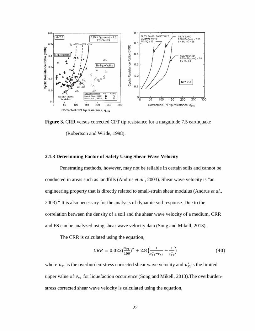
The left side of the Figure 3 is a graph of the CRR versus corrected CPT tip

resistance for a magnitude 7.5 earthquake (Robertson and Wride, 1998). The filled in

markers represent liquefaction while the blank markers represent no liquefaction. Soils

susceptible to liquefaction tend to fall on the left side of the limiting shear strain line, and

no liquefaction markers are denser on the right side of the line. The higher the tip

resistance, the less likely liquefaction will occur. The right side of Figure 3 is the same

graph different with soil types denoted. Silty sand to sandy silt is plotted on the far left,

followed by silty sand and clean sand on the far right (Robertson and Wride, 1998).

22

Figure 3. CRR versus corrected CPT tip resistance for a magnitude 7.5 earthquake

(Robertson and Wride, 1998).

2.1.3 Determining Factor of Safety Using Shear Wave Velocity

Penetrating methods, however, may not be reliable in certain soils and cannot be

conducted in areas such as landfills (Andrus et al., 2003). Shear wave velocity is "an

engineering property that is directly related to small-strain shear modulus (Andrus et al.,

2003)." It is also necessary for the analysis of dynamic soil response. Due to the

correlation between the density of a soil and the shear wave velocity of a medium, CRR

and FS can be analyzed using shear wave velocity data (Song and Mikell, 2013).

The CRR is calculated using the equation,

𝐶𝑅𝑅 = 0.022(𝑣𝑠1

100)2 + 2.8 (

1

𝑣𝑠1∗ −𝑣𝑠1

−1

𝑣𝑠1∗ ) (40)

where 𝑣𝑠1 is the overburden-stress corrected shear wave velocity and 𝑣𝑠1∗ is the limited

upper value of 𝑣𝑠1 for liquefaction occurrence (Song and Mikell, 2013).The overburden-

stress corrected shear wave velocity is calculated using the equation,

23

𝑉𝑠1 = 𝑉𝑠(𝑃𝑎

𝜎𝑣𝑜′)0.25 (41)

where 𝑃𝑎is the atmospheric pressure, i.e. 100 kPa (Song and Mikell, 2013).

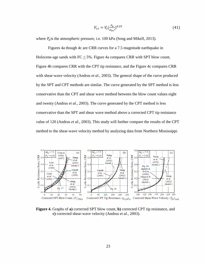
Figures 4a though 4c are CRR curves for a 7.5 magnitude earthquake in

Holocene-age sands with FC < 5%. Figure 4a compares CRR with SPT blow count,

Figure 4b compares CRR with the CPT tip resistance, and the Figure 4c compares CRR

with shear-wave velocity (Andrus et al., 2003). The general shape of the curve produced

by the SPT and CPT methods are similar. The curve generated by the SPT method is less

conservative than the CPT and shear wave method between the blow count values eight

and twenty (Andrus et al., 2003). The curve generated by the CPT method is less

conservative than the SPT and shear wave method above a corrected CPT tip resistance

value of 120 (Andrus et al., 2003). This study will further compare the results of the CPT

method to the shear-wave velocity method by analyzing data from Northern Mississippi.

Figure 4. Graphs of a) corrected SPT blow count, b) corrected CPT tip resistance, and

c) corrected shear-wave velocity (Andrus et al., 2003).

24

3.0Northern Mississippi Delta Data

A liquefaction susceptibility study of Desoto, Tunica, and Tate County,

Mississippi was conducted by Dr. Chung R. Song and Nathan Mikell from the University

of Mississippi Civil Engineering Department. This study will closely follow their report.

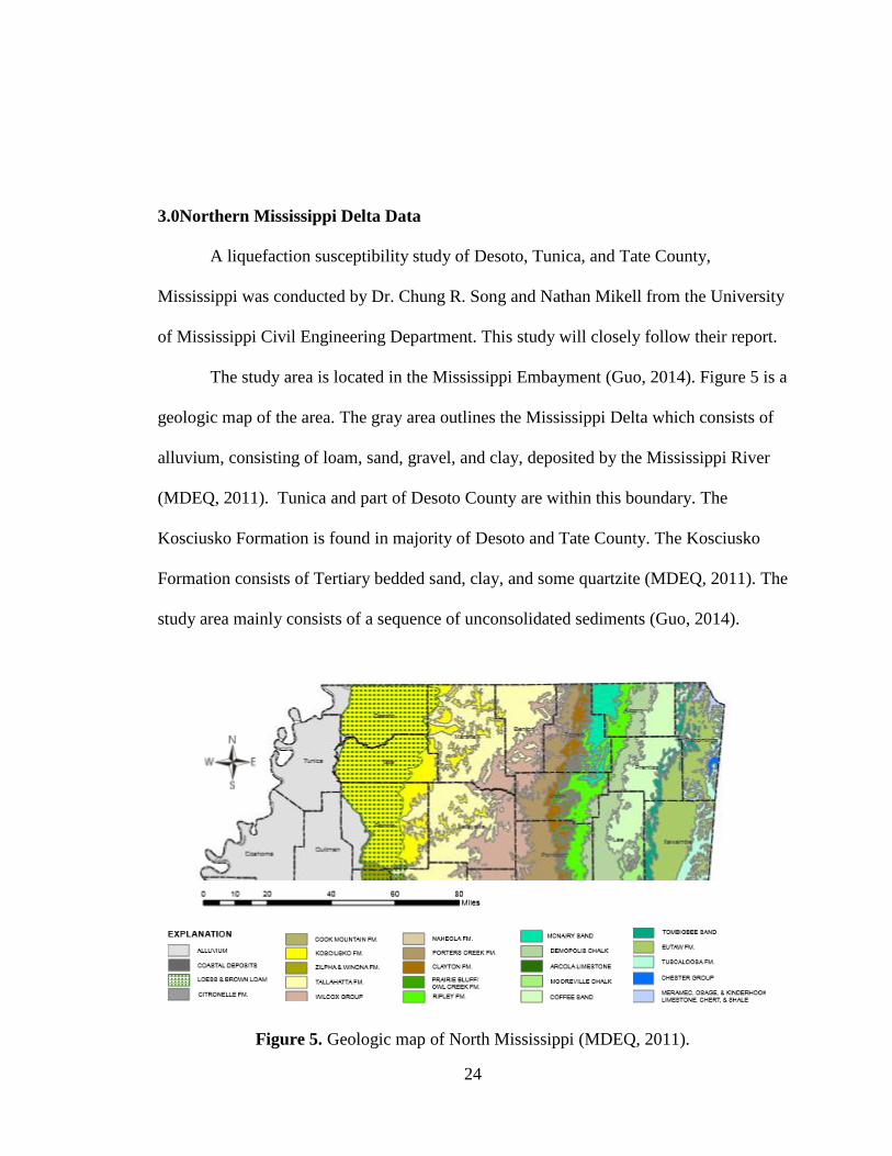
The study area is located in the Mississippi Embayment (Guo, 2014). Figure 5 is a

geologic map of the area. The gray area outlines the Mississippi Delta which consists of

alluvium, consisting of loam, sand, gravel, and clay, deposited by the Mississippi River

(MDEQ, 2011). Tunica and part of Desoto County are within this boundary. The

Kosciusko Formation is found in majority of Desoto and Tate County. The Kosciusko

Formation consists of Tertiary bedded sand, clay, and some quartzite (MDEQ, 2011). The

study area mainly consists of a sequence of unconsolidated sediments (Guo, 2014).

Figure 5. Geologic map of North Mississippi (MDEQ, 2011).

25

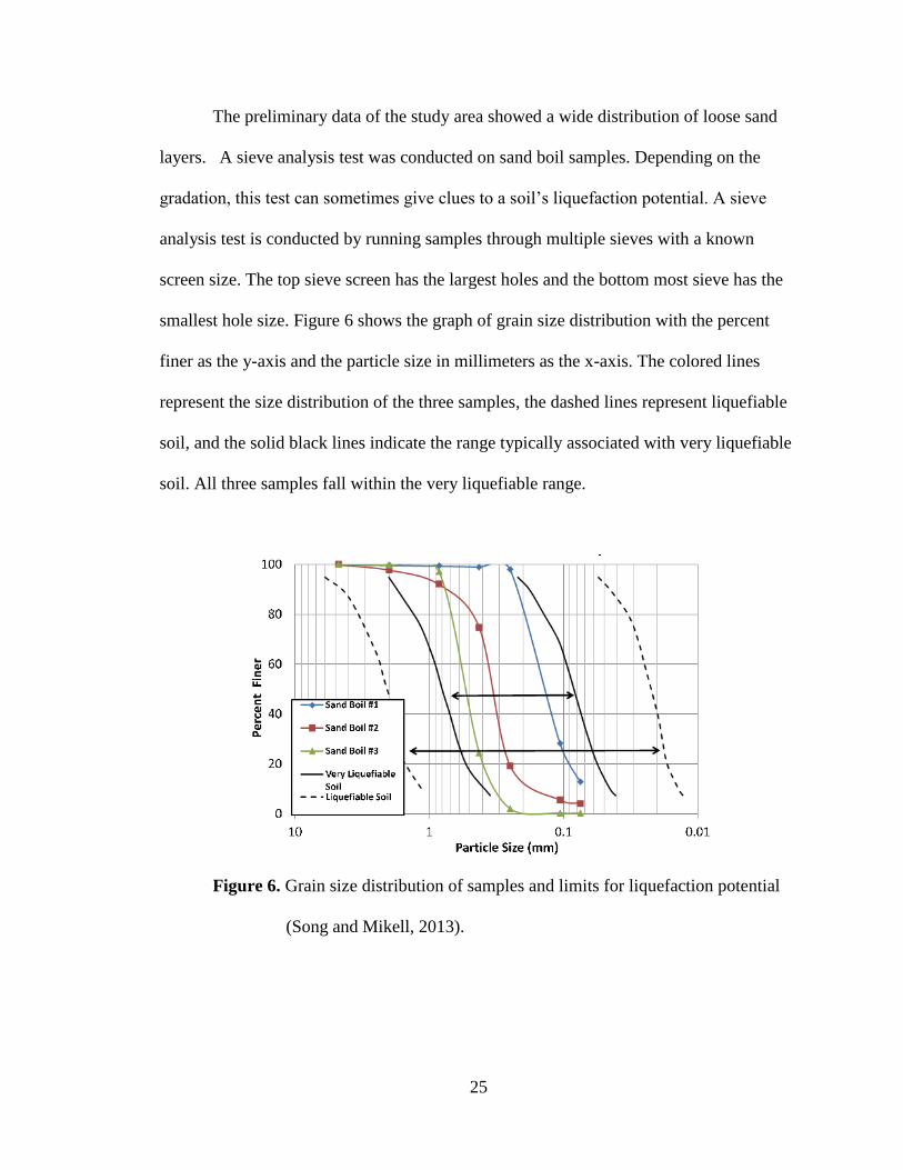
The preliminary data of the study area showed a wide distribution of loose sand

layers. A sieve analysis test was conducted on sand boil samples. Depending on the

gradation, this test can sometimes give clues to a soil’s liquefaction potential. A sieve

analysis test is conducted by running samples through multiple sieves with a known

screen size. The top sieve screen has the largest holes and the bottom most sieve has the

smallest hole size. Figure 6 shows the graph of grain size distribution with the percent

finer as the y-axis and the particle size in millimeters as the x-axis. The colored lines

represent the size distribution of the three samples, the dashed lines represent liquefiable

soil, and the solid black lines indicate the range typically associated with very liquefiable

soil. All three samples fall within the very liquefiable range.

Figure 6. Grain size distribution of samples and limits for liquefaction potential

(Song and Mikell, 2013).

26

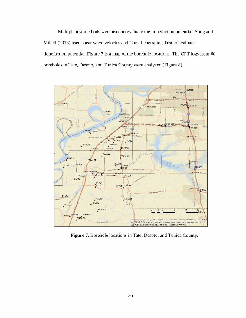
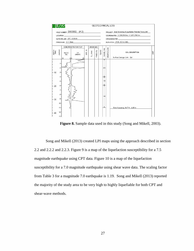
Multiple test methods were used to evaluate the liquefaction potential. Song and

Mikell (2013) used shear wave velocity and Cone Penetration Test to evaluate

liquefaction potential. Figure 7 is a map of the borehole locations. The CPT logs from 60

boreholes in Tate, Desoto, and Tunica County were analyzed (Figure 8).

Figure 7. Borehole locations in Tate, Desoto, and Tunica County.

27

Figure 8. Sample data used in this study (Song and Mikell, 2003).

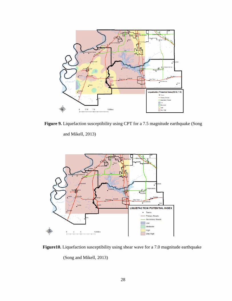
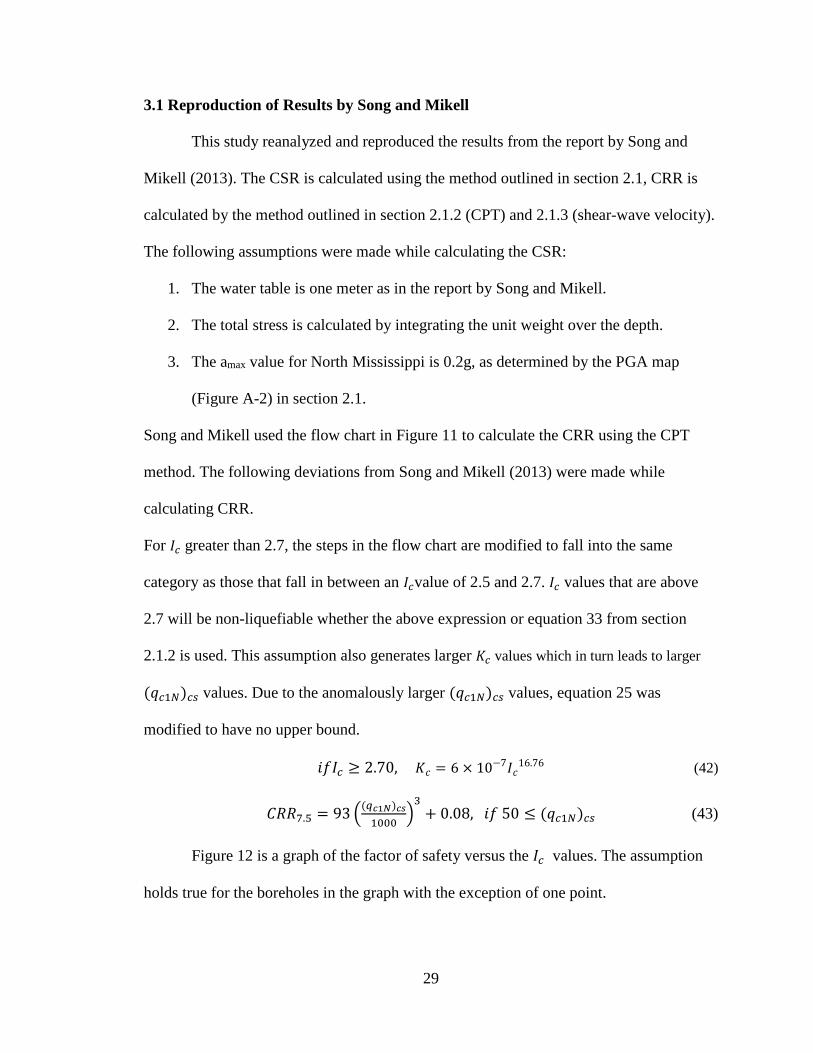
Song and Mikell (2013) created LPI maps using the approach described in section

2.2 and 2.2.2 and 2.2.3. Figure 9 is a map of the liquefaction susceptibility for a 7.5

magnitude earthquake using CPT data. Figure 10 is a map of the liquefaction

susceptibility for a 7.0 magnitude earthquake using shear wave data. The scaling factor

from Table 3 for a magnitude 7.0 earthquake is 1.19. Song and Mikell (2013) reported

the majority of the study area to be very high to highly liquefiable for both CPT and

shear-wave methods.

28

Figure 9. Liquefaction susceptibility using CPT for a 7.5 magnitude earthquake (Song

and Mikell, 2013)

Figure10. Liquefaction susceptibility using shear wave for a 7.0 magnitude earthquake

(Song and Mikell, 2013)

29

3.1 Reproduction of Results by Song and Mikell

This study reanalyzed and reproduced the results from the report by Song and

Mikell (2013). The CSR is calculated using the method outlined in section 2.1, CRR is

calculated by the method outlined in section 2.1.2 (CPT) and 2.1.3 (shear-wave velocity).

The following assumptions were made while calculating the CSR:

1. The water table is one meter as in the report by Song and Mikell.

2. The total stress is calculated by integrating the unit weight over the depth.

3. The amax value for North Mississippi is 0.2g, as determined by the PGA map

(Figure A-2) in section 2.1.

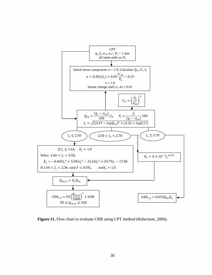
Song and Mikell used the flow chart in Figure 11 to calculate the CRR using the CPT

method. The following deviations from Song and Mikell (2013) were made while

calculating CRR.

For 𝐼𝑐 greater than 2.7, the steps in the flow chart are modified to fall into the same

category as those that fall in between an 𝐼𝑐value of 2.5 and 2.7. 𝐼𝑐 values that are above

2.7 will be non-liquefiable whether the above expression or equation 33 from section

2.1.2 is used. This assumption also generates larger 𝐾𝑐 values which in turn leads to larger

(𝑞𝑐1𝑁)𝑐𝑠 values. Due to the anomalously larger (𝑞𝑐1𝑁)𝑐𝑠 values, equation 25 was

modified to have no upper bound.

𝑖𝑓𝐼𝑐 ≥ 2.70, 𝐾𝑐 = 6 × 10−7𝐼𝑐16.76 (42)

𝐶𝑅𝑅7.5 = 93 ((𝑞𝑐1𝑁)𝑐𝑠

1000)

3

+ 0.08, 𝑖𝑓 50 ≤ (𝑞𝑐1𝑁)𝑐𝑠 (43)

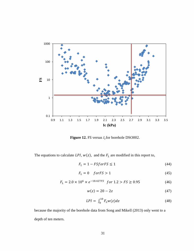
Figure 12 is a graph of the factor of safety versus the 𝐼𝑐 values. The assumption

holds true for the boreholes in the graph with the exception of one point.

30

CPT

qt, fs, σvo, σvo', Pa = 1 atm

all same units as Pa

Initial stress component: n = 1.0; Calculate Qtn, Fr, Ic

𝑛 = 0.381(Ic) + 0.05𝜎 ′

𝑣0

Pa

− 0.15

n ≤ 1.0

Iterate change until n2 Δn ≤ 0.01

𝐶𝑁 = (𝑃𝑎

𝜎𝑣0′ )

𝑛

𝑄𝑡𝑛 =(𝑞𝑐 − 𝜎𝑣𝑜)

100𝐶𝑁 𝐹𝑟 =

𝑓𝑠

(𝑞𝑐 − 𝜎𝑣𝑜)100

𝐼𝑐 = √[(3.47 − 𝑙𝑜𝑔𝑄𝑡𝑛)2 + (1.22 + 𝑙𝑜𝑔𝐹𝑟)2]

𝐼𝑓𝐼𝑐 ≤ 1.64, 𝐾𝑐 = 1.0

When 1.64 < 𝐼𝑐 < 2.60,

𝐾𝑐 = −0.403𝐼𝑐 4 + 5.581𝐼𝑐

3 − 21.63𝐼𝑐 2 + 33.75𝐼𝑐 − 17.88

If 1.64 < 𝐼𝑐 < 2.36 𝑎𝑛𝑑 𝐹 < 0.5%, 𝑠𝑒𝑡𝐾𝑐 = 1.0

𝐾𝑐 = 6 × 10−7𝐼𝑐16.76

𝑄𝑡𝑛,𝑐𝑠 = 𝐾𝑐𝑄𝑡𝑛

𝐶𝑅𝑅7.5 = 93 (𝑄𝑡𝑛,𝑐𝑠

1000)

3

+ 0.08

50 ≤ 𝑄𝑡𝑛,𝑐𝑠 ≤ 160

𝐶𝑅𝑅7.5 = 0.053𝑄𝑡𝑛𝐾𝛼

Ic ≤ 2.50 2.50 < Ic < 2.70 Ic ≥ 2.70

Figure 11. Flow chart to evaluate CRR using CPT method (Robertson, 2009).

31

Figure 12. FS versus 𝐼𝑐for borehole DSO002.

The equations to calculate 𝐿𝑃𝐼, 𝑤(𝑧), and the 𝐹𝐿 are modified in this report to,

𝐹𝐿 = 1 − 𝐹𝑆𝑓𝑜𝑟𝐹𝑆 ≤ 1 (44)

𝐹𝐿 = 0 𝑓𝑜𝑟𝐹𝑆 > 1 (45)

𝐹𝐿 = 2.0 × 106 × 𝑒−18.427𝐹𝑆 𝑓𝑜𝑟 1.2 > 𝐹𝑆 ≥ 0.95 (46)

𝑤(𝑧) = 20 − 2𝑧 (47)

𝐿𝑃𝐼 = ∫ 𝐹𝐿𝑤(𝑧)𝑑𝑧10

0 (48)

because the majority of the borehole data from Song and Mikell (2013) only went to a

depth of ten meters.

0.1

1

10

100

1000

0.9 1.1 1.3 1.5 1.7 1.9 2.1 2.3 2.5 2.7 2.9 3.1 3.3 3.5

FS

Ic (kPa)

32

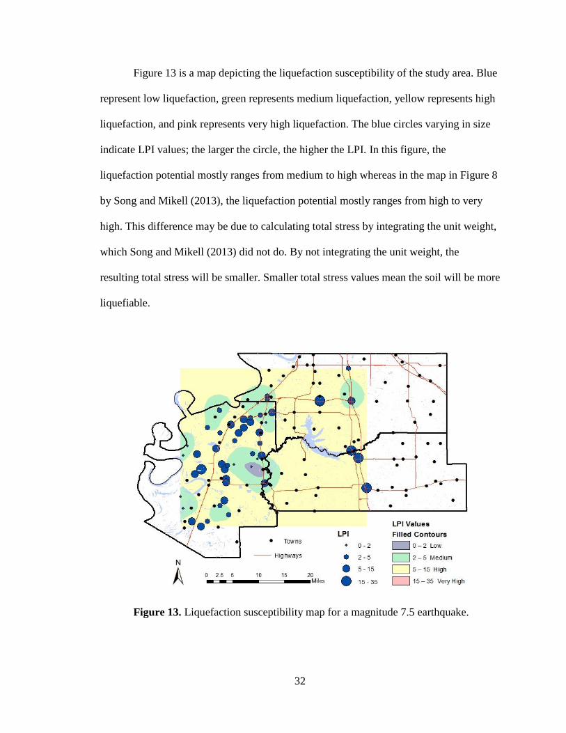
Figure 13 is a map depicting the liquefaction susceptibility of the study area. Blue

represent low liquefaction, green represents medium liquefaction, yellow represents high

liquefaction, and pink represents very high liquefaction. The blue circles varying in size

indicate LPI values; the larger the circle, the higher the LPI. In this figure, the

liquefaction potential mostly ranges from medium to high whereas in the map in Figure 8

by Song and Mikell (2013), the liquefaction potential mostly ranges from high to very

high. This difference may be due to calculating total stress by integrating the unit weight,

which Song and Mikell (2013) did not do. By not integrating the unit weight, the

resulting total stress will be smaller. Smaller total stress values mean the soil will be more

liquefiable.

Figure 13. Liquefaction susceptibility map for a magnitude 7.5 earthquake.

33

3.2 Calculating LPI Using Average CSR

The purpose of this study is to create a hybrid method for calculating the LPI. It

aims to combine a non-invasive and more cost effective method of calculating the CRR

using surface shear wave data with and an average CSR determined using CPT data from

existing boreholes.

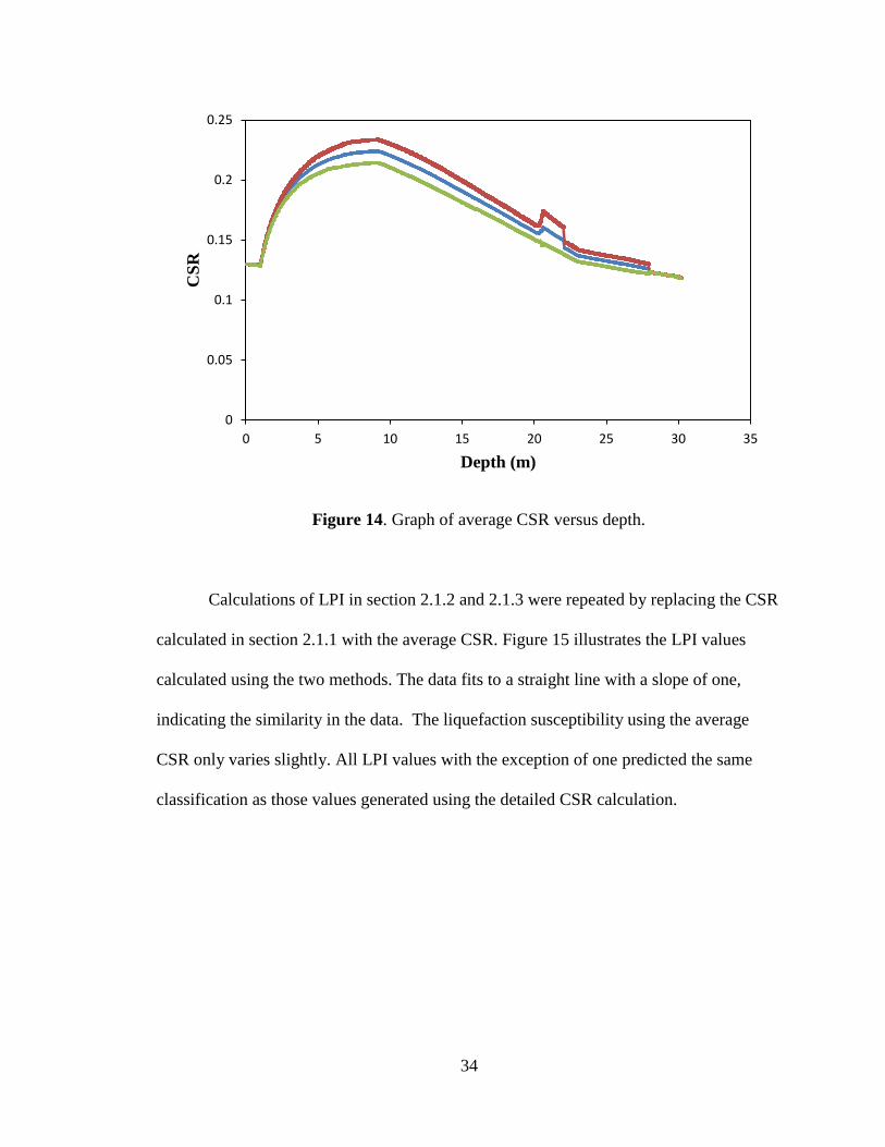
3.2.1 Calculating Average CSR

The CSR versus depth using CPT data is calculated for all 60 boreholes. The CSR

for each depth interval is averaged over all the boreholes. A standard deviation for the

average CPR versus depth is calculated. Figure 14 displays the average CSR versus depth

with the one standard deviation. Due to the low values of the standard deviation, this

calculation indicates small viability between the individual CSR versus depth. The

viability is less than 10%. An 𝑎𝑚𝑎𝑥 value of 0.2g is used in calculating the CSR values

because the borehole holes are located in Northern Mississippi. According to Figure 2,

this area has a peak acceleration value of 20 percent. Using the average CSR works in

this study appears feasible because the area is small enough that the 𝑎𝑚𝑎𝑥 is the same

throughout. This also indicates that the geology is fairly consistent with depth. The

inconsistency in Figure 14 after a depth of 20 meters is due to the limited amount of data

available past this depth.

34

Figure 14. Graph of average CSR versus depth.

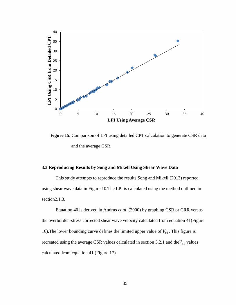
Calculations of LPI in section 2.1.2 and 2.1.3 were repeated by replacing the CSR

calculated in section 2.1.1 with the average CSR. Figure 15 illustrates the LPI values

calculated using the two methods. The data fits to a straight line with a slope of one,

indicating the similarity in the data. The liquefaction susceptibility using the average

CSR only varies slightly. All LPI values with the exception of one predicted the same

classification as those values generated using the detailed CSR calculation.

0

0.05

0.1

0.15

0.2

0.25

0 5 10 15 20 25 30 35

CS

R

Depth (m)

35

Figure 15. Comparison of LPI using detailed CPT calculation to generate CSR data

and the average CSR.

3.3 Reproducing Results by Song and Mikell Using Shear Wave Data

This study attempts to reproduce the results Song and Mikell (2013) reported

using shear wave data in Figure 10.The LPI is calculated using the method outlined in

section2.1.3.

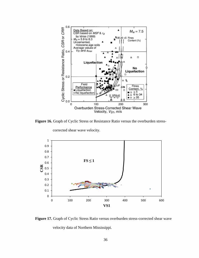
Equation 40 is derived in Andrus et al. (2000) by graphing CSR or CRR versus

the overburden-stress corrected shear wave velocity calculated from equation 41(Figure

16).The lower bounding curve defines the limited upper value of 𝑉𝑠1. This figure is

recreated using the average CSR values calculated in section 3.2.1 and the𝑉𝑠1 values

calculated from equation 41 (Figure 17).

0

5

10

15

20

25

30

35

40

0 5 10 15 20 25 30 35 40

LP

I U

sin

g C

SR

fro

m D

etail

ed C

PT

LPI Using Average CSR

36

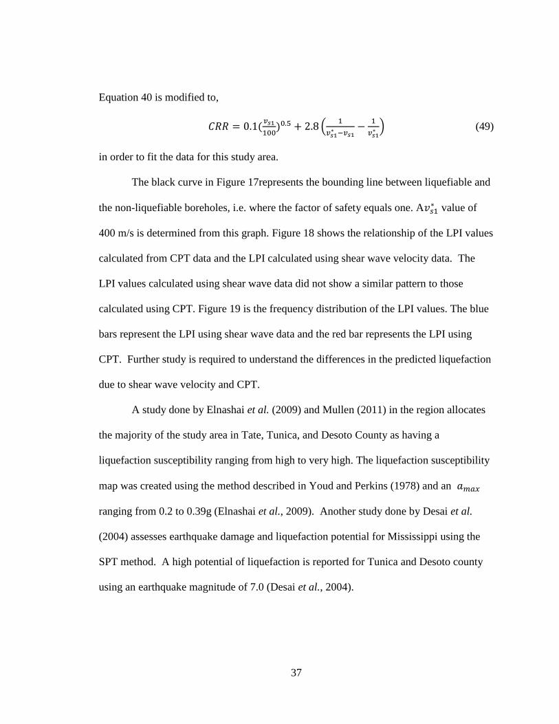
Figure 16. Graph of Cyclic Stress or Resistance Ratio versus the overburden stress-

corrected shear wave velocity.

Figure 17. Graph of Cyclic Stress Ratio versus overburden stress-corrected shear wave

velocity data of Northern Mississippi.

0

0.1

0.2

0.3

0.4

0.5

0.6

0.7

0.8

0.9

1

0 100 200 300 400 500 600

CS

R

VS1

FS ≤ 1

37

Equation 40 is modified to,

𝐶𝑅𝑅 = 0.1(𝑣𝑠1

100)0.5 + 2.8 (

1

𝑣𝑠1∗ −𝑣𝑠1

−1

𝑣𝑠1∗ ) (49)

in order to fit the data for this study area.

The black curve in Figure 17represents the bounding line between liquefiable and

the non-liquefiable boreholes, i.e. where the factor of safety equals one. A𝑣𝑠1∗ value of

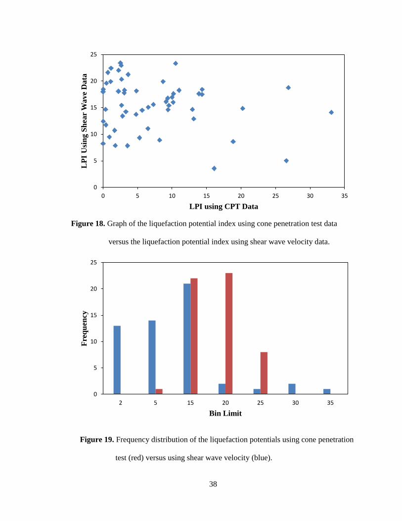
400 m/s is determined from this graph. Figure 18 shows the relationship of the LPI values

calculated from CPT data and the LPI calculated using shear wave velocity data. The

LPI values calculated using shear wave data did not show a similar pattern to those

calculated using CPT. Figure 19 is the frequency distribution of the LPI values. The blue

bars represent the LPI using shear wave data and the red bar represents the LPI using

CPT. Further study is required to understand the differences in the predicted liquefaction

due to shear wave velocity and CPT.

A study done by Elnashai et al. (2009) and Mullen (2011) in the region allocates

the majority of the study area in Tate, Tunica, and Desoto County as having a

liquefaction susceptibility ranging from high to very high. The liquefaction susceptibility

map was created using the method described in Youd and Perkins (1978) and an 𝑎𝑚𝑎𝑥

ranging from 0.2 to 0.39g (Elnashai et al., 2009). Another study done by Desai et al.

(2004) assesses earthquake damage and liquefaction potential for Mississippi using the

SPT method. A high potential of liquefaction is reported for Tunica and Desoto county

using an earthquake magnitude of 7.0 (Desai et al., 2004).

38

Figure 18. Graph of the liquefaction potential index using cone penetration test data

versus the liquefaction potential index using shear wave velocity data.

Figure 19. Frequency distribution of the liquefaction potentials using cone penetration

test (red) versus using shear wave velocity (blue).

0

5

10

15

20

25

0 5 10 15 20 25 30 35

LP

I U

sin

g S

hea

r W

ave

Data

LPI using CPT Data

0

5

10

15

20

25

2 5 15 20 25 30 35

Fre

qu

ency

Bin Limit

39

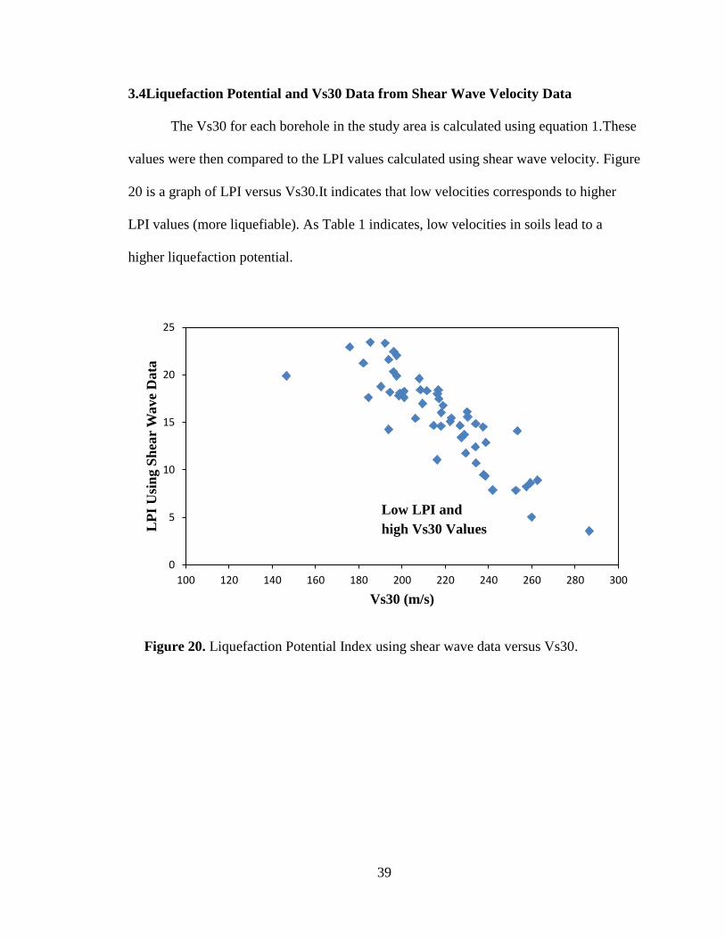
3.4Liquefaction Potential and Vs30 Data from Shear Wave Velocity Data

The Vs30 for each borehole in the study area is calculated using equation 1.These

values were then compared to the LPI values calculated using shear wave velocity. Figure

20 is a graph of LPI versus Vs30.It indicates that low velocities corresponds to higher

LPI values (more liquefiable). As Table 1 indicates, low velocities in soils lead to a

higher liquefaction potential.

Figure 20. Liquefaction Potential Index using shear wave data versus Vs30.

0

5

10

15

20

25

100 120 140 160 180 200 220 240 260 280 300

LP

I U

sin

g S

hea

r W

ave

Data

Vs30 (m/s)

Low LPI and

high Vs30 Values

40

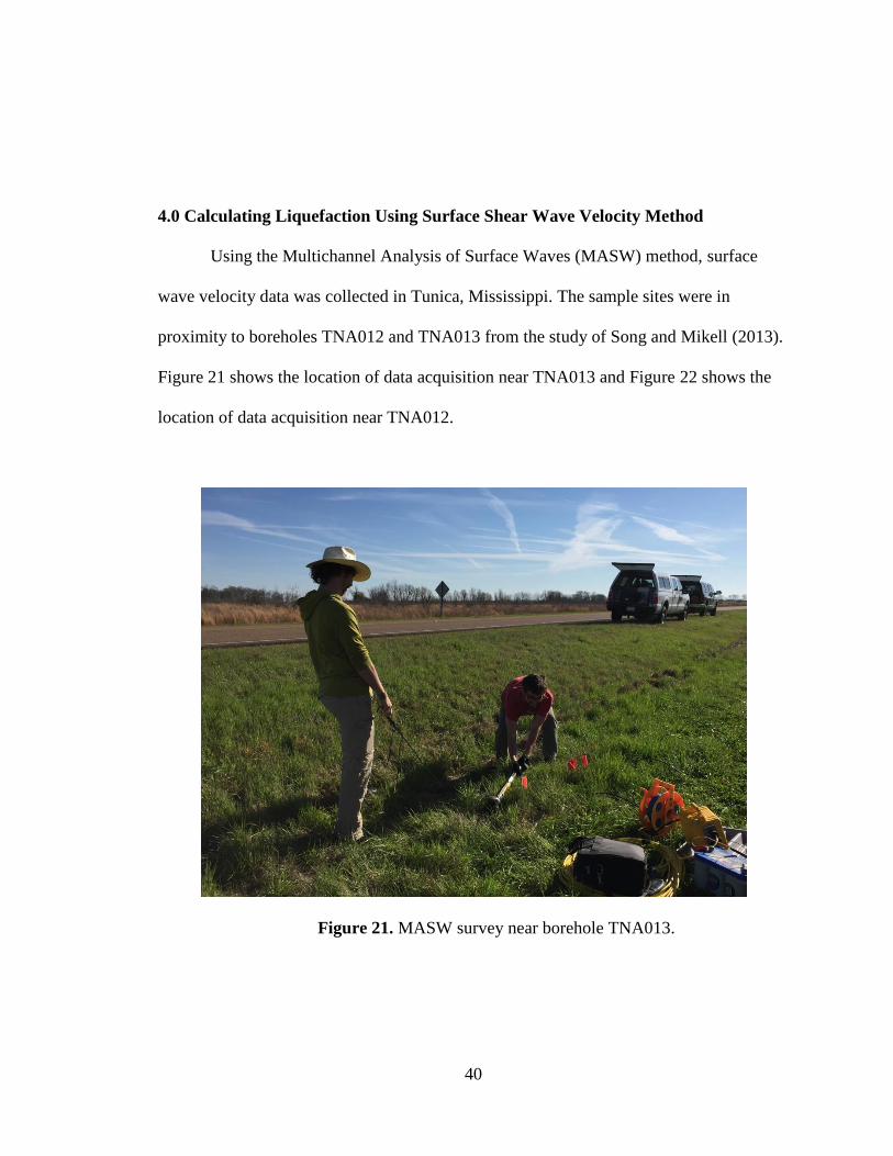
4.0 Calculating Liquefaction Using Surface Shear Wave Velocity Method

Using the Multichannel Analysis of Surface Waves (MASW) method, surface

wave velocity data was collected in Tunica, Mississippi. The sample sites were in

proximity to boreholes TNA012 and TNA013 from the study of Song and Mikell (2013).

Figure 21 shows the location of data acquisition near TNA013 and Figure 22 shows the

location of data acquisition near TNA012.

Figure 21. MASW survey near borehole TNA013.

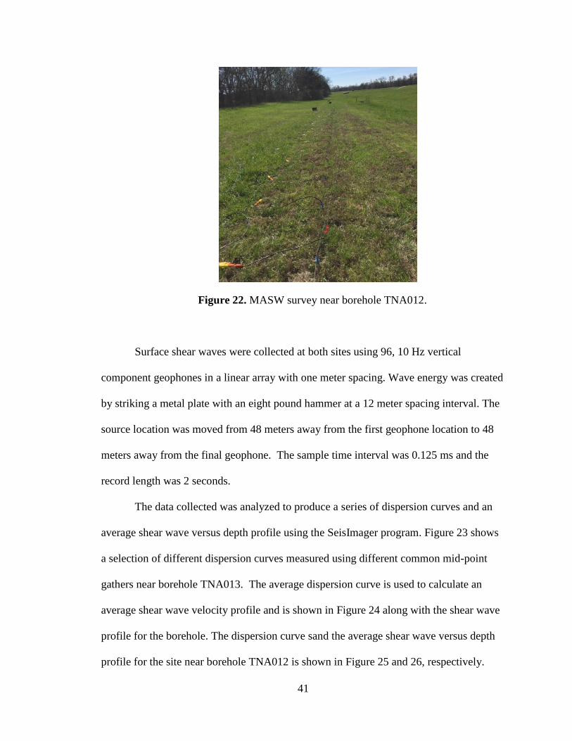
41

Figure 22. MASW survey near borehole TNA012.

Surface shear waves were collected at both sites using 96, 10 Hz vertical

component geophones in a linear array with one meter spacing. Wave energy was created

by striking a metal plate with an eight pound hammer at a 12 meter spacing interval. The

source location was moved from 48 meters away from the first geophone location to 48

meters away from the final geophone. The sample time interval was 0.125 ms and the

record length was 2 seconds.

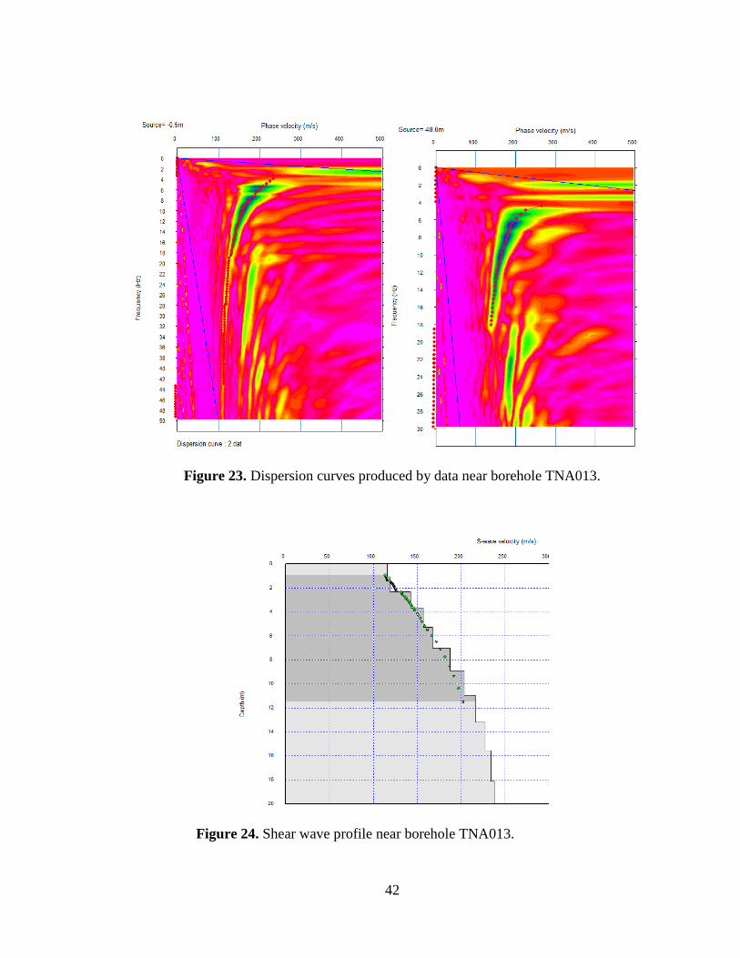
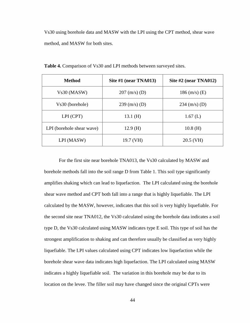
The data collected was analyzed to produce a series of dispersion curves and an

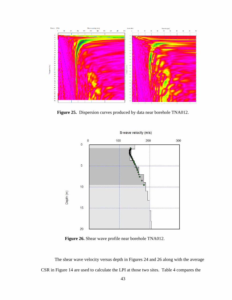
average shear wave versus depth profile using the SeisImager program. Figure 23 shows

a selection of different dispersion curves measured using different common mid-point

gathers near borehole TNA013. The average dispersion curve is used to calculate an

average shear wave velocity profile and is shown in Figure 24 along with the shear wave

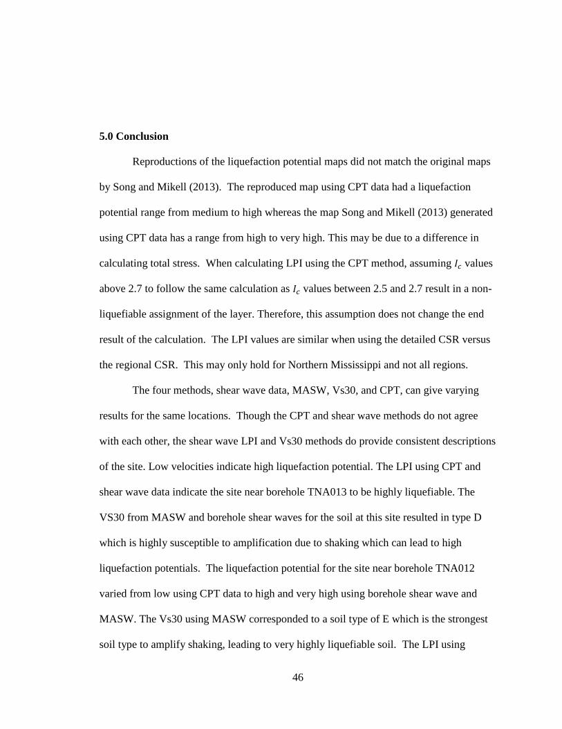
profile for the borehole. The dispersion curve sand the average shear wave versus depth

profile for the site near borehole TNA012 is shown in Figure 25 and 26, respectively.

42

Figure 23. Dispersion curves produced by data near borehole TNA013.

Figure 24. Shear wave profile near borehole TNA013.

43

Figure 25. Dispersion curves produced by data near borehole TNA012.

Figure 26. Shear wave profile near borehole TNA012.

The shear wave velocity versus depth in Figures 24 and 26 along with the average

CSR in Figure 14 are used to calculate the LPI at those two sites. Table 4 compares the

44

Vs30 using borehole data and MASW with the LPI using the CPT method, shear wave

method, and MASW for both sites.

Table 4. Comparison of Vs30 and LPI methods between surveyed sites.

Method Site #1 (near TNA013) Site #2 (near TNA012)

Vs30 (MASW) 207 (m/s) (D) 186 (m/s) (E)

Vs30 (borehole) 239 (m/s) (D) 234 (m/s) (D)

LPI (CPT) 13.1 (H) 1.67 (L)

LPI (borehole shear wave) 12.9 (H) 10.8 (H)

LPI (MASW) 19.7 (VH) 20.5 (VH)

For the first site near borehole TNA013, the Vs30 calculated by MASW and

borehole methods fall into the soil range D from Table 1. This soil type significantly

amplifies shaking which can lead to liquefaction. The LPI calculated using the borehole

shear wave method and CPT both fall into a range that is highly liquefiable. The LPI

calculated by the MASW, however, indicates that this soil is very highly liquefiable. For

the second site near TNA012, the Vs30 calculated using the borehole data indicates a soil

type D, the Vs30 calculated using MASW indicates type E soil. This type of soil has the

strongest amplification to shaking and can therefore usually be classified as very highly

liquefiable. The LPI values calculated using CPT indicates low liquefaction while the

borehole shear wave data indicates high liquefaction. The LPI calculated using MASW

indicates a highly liquefiable soil. The variation in this borehole may be due to its

location on the levee. The filler soil may have changed since the original CPTs were

45

collected. If the soil is newer and not as compacted, it would have a higher potential to

liquefy.

46

5.0 Conclusion

Reproductions of the liquefaction potential maps did not match the original maps

by Song and Mikell (2013). The reproduced map using CPT data had a liquefaction

potential range from medium to high whereas the map Song and Mikell (2013) generated

using CPT data has a range from high to very high. This may be due to a difference in

calculating total stress. When calculating LPI using the CPT method, assuming 𝐼𝑐 values

above 2.7 to follow the same calculation as 𝐼𝑐 values between 2.5 and 2.7 result in a non-

liquefiable assignment of the layer. Therefore, this assumption does not change the end

result of the calculation. The LPI values are similar when using the detailed CSR versus

the regional CSR. This may only hold for Northern Mississippi and not all regions.

The four methods, shear wave data, MASW, Vs30, and CPT, can give varying

results for the same locations. Though the CPT and shear wave methods do not agree

with each other, the shear wave LPI and Vs30 methods do provide consistent descriptions

of the site. Low velocities indicate high liquefaction potential. The LPI using CPT and

shear wave data indicate the site near borehole TNA013 to be highly liquefiable. The

VS30 from MASW and borehole shear waves for the soil at this site resulted in type D

which is highly susceptible to amplification due to shaking which can lead to high

liquefaction potentials. The liquefaction potential for the site near borehole TNA012

varied from low using CPT data to high and very high using borehole shear wave and

MASW. The Vs30 using MASW corresponded to a soil type of E which is the strongest

soil type to amplify shaking, leading to very highly liquefiable soil. The LPI using

47

MASW provides a more conservative estimate that indicates this site is very highly

liquefiable. The variation of the liquefaction potential near this borehole may be due to its

location on the levee. The soil at the location may have changed since the time the CPTs

used in the study by Song and Mikell (2013) were acquired.

Northern Mississippi with all methods, however, is mostly highly liquefiable.

Liquefaction susceptibility using the LPI value can be calculated using several different

methods. Though non-invasive methods such as refraction and MASW are cheaper, the

LPI calculation is more conservative.

48

BIBILIOGRAPHY

49

Andrus, R. D., Piratheepan, P., Ellis, B. S., Zhang, J., and Juang, C. H., "Comparing

Liquefaction Evaluation Methods Using Penetration-VS Relationships."

Department of Civil Engineering, Clemson University, 2003.

Andrus, R. D., Stokoe, H. K., B. S., "Liquefaction Resistance of Soil from Shear Wave

Velocity." Journal of Geotechnical and Geoenvironmental Engineering, 2000.

Braile, L. W., Hinze, W. J., Keller, G. R., Lidiak, E. G., and Sexton, J. L. "Tectonic

Development of the New Madrid Rift Complex, Mississippi Embayment, North

America." Tectonophysics 131.1-2: 1-21. Print, 1986.

Central United States Earthquake Consortium. "Earthquake Information: New Madrid

Seismic Zone." Web, 2014

Desai, K., Mullen, C., and George, K. P. "Earthquake Damage Assessment and

Liquefaction Potential for the State of Mississippi." University of Mississippi,

2004.

Elnashai, A. M., Jefferson, T., Fiedrich, F., Cleveland, L. J., and Gress, T. "Impact of

New Madrid Seismic Zone Earthquakes on the Central USA." Mid-America

Earthquake Center. University of Illinois, 2009.

Fillingim, M. "Intraplate Earthquakes: Possible Mechanisms for the New Madrid and

Charleston Earthquakes." Intraplate Earthquakes: Possible Mechanisms for the

New Madrid and Charleston Earthquakes. University of California at Berkeley,

1999.

Geotechdata.info. "Standard Penetration Test." Geotechdata.info, 2013.

50

Greene, M., Power, M., and Youd, L. T. "Liquefaction: What It Is and What to Do about

It." Earthquake Basics 1: 1-8. Innovative Technology Transfer Committee of the

Earthquake Engineering Research Institute, 1994.

Guo, Z., Aydin, A., Kuszmaul, J. "Microtremor Recordings in Northern Mississippi."

Department of Geology and Geological Engineering, University of Mississippi,

2014.

Holzer, T. L., Noce, T. E., Bennett, M. J. "Scenario Liquefaction Hazard Maps of Santa

Clara Valley, Northern California." Bulletin of the Seismological Society of

America, Vol. 99, No. 1, 367–381, 2009.

Iwasaki, T., Tatsuoka, D., Tokida, K., and Yasuda, S. A practical Method for Assessing

Soil Liquefaction Potential Based on Case Studies at Various Sites in Japan, in

Proc. 2nd Int. Conf. on Microzonation, San Francisco, 885-896, 1978.

Johansson, J. "Initiation of Liquefaction: Why Does Liquefaction Occur?" Department of

Civil Engineering, University of Washington, 2000.

Johari, A., and Khodaparast, A. R. "Modeling of Probability Liquefaction Based on

Standard Penetration Tests Using the Jointly Distributed Random Variables

Method." Engineering Geology 158: 1-14. Print, 2013.

Lowrie, W. Fundamentals of Geophysics: "Seismology and the Internal Structure of the

Earth." Cambridge University Press, UK, 83-63, 1997.

Missouri Department of Natural Resources. "Facts about the New Madrid Seismic Zone."

Missouri Department of Natural Resources, n.d. Web, 2014.

Mississippi Department of Environment Quality. Geologic maps and data for Mississippi.

MDEQ, 2011.

51

Mullen, C. "Seismic Vulnerability of Critical Bridges in North Mississippi." Mississippi

Emergency Management Agency, 2011.

Odum, J. K. "Near Surface Shear Wave Velocity versus Depth Profiles, Vs30, and

NEHRP Classifications for 27 Sites in Puerto Rico." USGS. U.S. Geological

Survey, 2007.

Park, C. B., Miller, D. R., Xia, J., Ivanov, J. "Multichannel Analysis of Surface Waves

(MASW)—Active and Passive Methods." The Leading Edge, 2007.

Rauch, A. F. "EPOLLS: An Empirical Method for Predicting Surface Displacements Due

to Liquefaction-Induced Lateral Spreading in Earthquakes." Diss. Virginia

Polytechnic Institute and State University, 1997.N.p.: Digital Library and

Archives. Print, 1997.

Robertson, P. K. and Wride, C. E. (Fear). "Evaluating Cyclic Liquefaction Potential

Using the Cone Penetration Test." Canadian Geotechnical Journal 35.3: 442-59.

Print, 1998.

Robertson, P.K. and Fear, C.E., “Soil liquefaction and its evaluation based on SPT and

CPT.” Liquefaction Workshop, 1996.

Rodgers, J. D. "Fundamentals of Cone Penetrometer Test (CPT) Soundings." Missouri

University of Science and Technology, 2004.

Silva, W. "Ground Motion and Liquefaction Simulation of the 1886 Charleston, South

Carolina, Earthquake." Bulletin of the Seismological Society of America 93.6:

2717-736. Print, 2003.

52

Song, C. R., and Mikell, N. "Earthquake and Piping Hazard Assessment for Desoto,

Tunica, and Tate County, Mississippi." Department of Civil Engineering,

University of Mississippi, 2013.

Spall, H. "Earthquakes and Plate Tectonics." Earthquakes and Plate Tectonics. USGS,

1976.

United States Geological Survey. "Earthquake Hazards 101: The Basics." U.S.

Geological Survey, 2015.

United States Geological Survey. "Earthquake Hazards 201: Technical Q&A." U.S.

Geological Survey, 2014.

United States Geological Survey. "History of Earthquakes." U.S. Geological Survey,

2012.

United States Geological Survey. "Soil Type and Shaking Hazard in the San Francisco

Bay Area." Soil Type and Shaking Hazard in the San Francisco Bay Area. U.S.

Geological Survey, 2012.

Youd, T.L. and Perkins, D. M. "Mapping of Liquefaction Induced Ground Failure

Potential." Journal of the Geotechnical Engineering Division, ASCE. v 104, n 4,

433-446, 1978.