Embed Size (px)
Citation preview
This content has been downloaded from IOPscience. Please scroll down to see the full text.
Download details:
IP Address: 134.153.184.170
This content was downloaded on 18/07/2014 at 23:44
Please note that terms and conditions apply.
Calculation of the Energy Levels to High States in Atomic Oxygen
View the table of contents for this issue, or go to the journal homepage for more
2004 Phys. Scr. 69 398
(http://iopscience.iop.org/1402-4896/69/5/007)
Home Search Collections Journals About Contact us My IOPscience
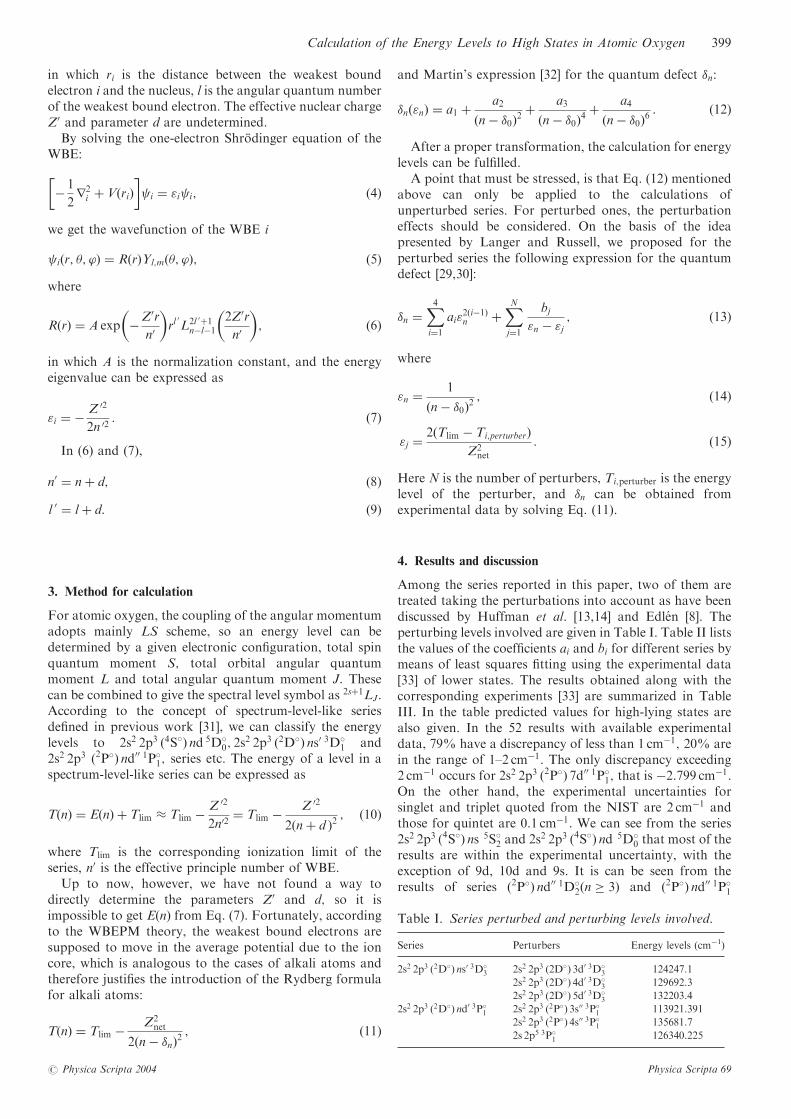
Calculation of the Energy Levels to High States in Atomic Oxygen
J. Fan, N. W. Zheng�, D. X. Ma and T. Wang
Department of Chemistry, University of Science and Technology of China, Hefei, Anhui 230026, P.R. China
Received September 9, 2003; accepted in revised form November 7, 2003
PACS Ref: 31.15.�p, 31.15.Ct
Abstract
Energy levels of configuration 2s2 2p3 ð4S�; 2D�; 2P�Þ nl in atomic oxygen are
reported within the weakest bound electron potential model theory (WBEPM
theory). In the calculations interactions between different series are explicitly
accounted for by introducing a combined quantum defect formula. The present
results show a reasonably good agreement with the critically evaluated NIST
data. Furthermore, predictions of energy levels are extended to high Rydberg
states.
1. Introduction
For the significant role atomic oxygen plays in the studiesconcerning a vast area such as the earth (includingatmosphere) and other celestial objects, it is important toobtain detailed structure information of atomic oxygenwhether experimentally or theoretically. Numerous studiesusing a variety of methods have been reported [1–6]. Theenergy levels for atomic oxygen given by Moore [7] hadbeen taken from Edlen’s paper [8], in which he had revisedand extended the earlier work by others [9–12]. Huffmanet al. [13,14] reported nine absorption series of ground-state atomic oxygen and eight series with the metastableoxygen atoms 2P4 1D2 and 2P4 1S0 as the lower states.Emission spectra were studied by Eriksson and Isberg[15,16] who gave several series of quintet terms besidessinglet and triplet. Rudd and Smith [17], Edward andCunningham [18] studied independently several series ofauto-ionizing atomic oxygen states.In respect of theoretical investigation on atomic energy
levels, many methods have been reported, among them areconfiguration interaction (CI) method [19,20], quantumdefect theory (QDT) [21,22], and multiconfigurationHartree–Fock (MCHF) method [23]. The applications,however, are sometimes limited to one or two valence-electron systems. Studies on many valence-electron systemsare restricted to lower states. When it comes to morecomplex atoms, especially the high Rydberg states foratoms and highly-ionized states for ions, the accuratetreatments for energy levels are quite difficult. This is alsotrue for atomic oxygen. As is well known the groundconfiguration of atomic oxygen is 1s22s22p4; and the corecorrelation, core-valence correlation and interactionbetween different Rydberg series found in such an open-shell system bring about much difficulty to theoreticalcalculations. Pradhan and Saraph [24] evaluated Rydbergseries of neutral oxygen up to n ¼ 6 by the close-couplingmethod in the frozen-cores approximation and obtainedterm energies with the largest discrepancy of 35%. Hibbert
et al. [25] carried out CI calculations on energy levels (withn � 4) of neutral oxygen obtaining an error of about 0.01a.u. (about 2200 cm�1). Using the R-matrix method,Thomas et al. [26] calculated the energy levels of 16 statesarising from the 2s2 2p3 nl; n ¼ 3; 4; configuration andobtained the results of a similar accuracy to those fromHibbert. Similarly, Zatsarinny and Tayal [27] reported theenergy levels of O I with an accuracy of the order of 0.001a.u. (about 220 cm�1). This accuracy is clearly better thanthose from Hibbert et al. [25] and Thomas et al. [26].Although the size of the wavefunction expansions in thispaper is close to that used by Hibbert et al. and Thomaset al., however, much more different spectroscopic andcorrelated orbitals are used. Recently, results of Breit-Paulienergy levels are presented for levels up to 2p33d of atomicoxygen [28]. The difference between the computed energiesand the experiments is in the range 110–280 cm�1:
In this paper, we aim to precisely study within theWBEPM theory the regulation of the levels of configura-tion 2s2 2p3 ð4S�; 2D�; 2P�Þ nl in atomic oxygen by areasonable classification of excited levels and predict theenergy levels of high Rydberg states. For space reason, theresults listed here are up to principal quantum numbern ¼ 100:
2. Principle of calculation
Details of the WBEPM theory can be found in ourprevious papers [29,30], in which energy levels of thecarbon group and krypton have been studied withsatisfactory accuracy. In brief, the electrons in an atomor ion are supposed to be divided into weakest boundelectron (WBE) and non-weakest bound electrons(NWBEs) considering the tendency of being excited orionized, and each of the WBE can be treated as a one-electron problem. In addition, WBEPM theory treats theion core composed of NWBEs and nuclear as a whole, andthe WBE is supposed to move in the average potential dueto the ion core.
By the above consideration, as well as the effects ofshielding, penetration and polarization, we construct thepotential function for the WBE as
VðriÞ ¼ A
riþ B
r2i(in a.u.); ð1Þ
A ¼ �Z0; ð2Þ
B ¼ dðdþ 1Þ þ 2dl
2; ð3Þ�To whom correspondence should be addressed
e-mail: [email protected]
Physica Scripta. Vol. 69, 398–402, 2004
Physica Scripta 69 # Physica Scripta 2004
in which ri is the distance between the weakest boundelectron i and the nucleus, l is the angular quantum numberof the weakest bound electron. The effective nuclear chargeZ0 and parameter d are undetermined.By solving the one-electron Shrodinger equation of the
WBE:
� 1
2r2i þ VðriÞ
� � i ¼ "i i; ð4Þ
we get the wavefunction of the WBE i
iðr; �; ’Þ ¼ RðrÞYl;mð�; ’Þ; ð5Þwhere
RðrÞ ¼ A exp �Z0rn0
� �rl
0L2l 0þ1n�l�1
2Z0rn0
� �; ð6Þ
in which A is the normalization constant, and the energyeigenvalue can be expressed as
"i ¼ � Z 02
2n 02 : ð7Þ
In (6) and (7),
n0 ¼ nþ d; ð8Þl 0 ¼ lþ d: ð9Þ
3. Method for calculation
For atomic oxygen, the coupling of the angular momentumadopts mainly LS scheme, so an energy level can bedetermined by a given electronic configuration, total spinquantum moment S; total orbital angular quantummoment L and total angular quantum moment J: Thesecan be combined to give the spectral level symbol as 2sþ1LJ:According to the concept of spectrum-level-like seriesdefined in previous work [31], we can classify the energylevels to 2s2 2p3 ð4S�Þ nd 5D�
0; 2s2 2p3 ð2D�Þ ns0 3D�
1 and2s2 2p3 ð2P�Þ nd00 1P�
1; series etc. The energy of a level in aspectrum-level-like series can be expressed as
TðnÞ ¼ EðnÞ þ Tlim � Tlim � Z 02
2n02¼ Tlim � Z 02
2ðnþ d Þ2 ; ð10Þ
where Tlim is the corresponding ionization limit of theseries, n0 is the effective principle number of WBE.Up to now, however, we have not found a way to
directly determine the parameters Z0 and d; so it isimpossible to get EðnÞ from Eq. (7). Fortunately, accordingto the WBEPM theory, the weakest bound electrons aresupposed to move in the average potential due to the ioncore, which is analogous to the cases of alkali atoms andtherefore justifies the introduction of the Rydberg formulafor alkali atoms:
TðnÞ ¼ Tlim � Z2net
2ðn� �nÞ2; ð11Þ
and Martin’s expression [32] for the quantum defect �n:
�nð"nÞ ¼ a1 þ a2
ðn� �0Þ2þ a3
ðn� �0Þ4þ a4
ðn� �0Þ6: ð12Þ
After a proper transformation, the calculation for energylevels can be fulfilled.
A point that must be stressed, is that Eq. (12) mentionedabove can only be applied to the calculations ofunperturbed series. For perturbed ones, the perturbationeffects should be considered. On the basis of the ideapresented by Langer and Russell, we proposed for theperturbed series the following expression for the quantumdefect [29,30]:
�n ¼X4i¼1
ai"2ði�1Þn þ
XNj¼1
bj"n � "j ; ð13Þ
where
"n ¼ 1
ðn� �0Þ2; ð14Þ
"j ¼ 2ðTlim � Ti;perturberÞZ2
net
: ð15Þ
Here N is the number of perturbers, Ti;perturber is the energylevel of the perturber, and �n can be obtained fromexperimental data by solving Eq. (11).
4. Results and discussion
Among the series reported in this paper, two of them aretreated taking the perturbations into account as have beendiscussed by Huffman et al. [13,14] and Edlen [8]. Theperturbing levels involved are given in Table I. Table II liststhe values of the coefficients ai and bi for different series bymeans of least squares fitting using the experimental data[33] of lower states. The results obtained along with thecorresponding experiments [33] are summarized in TableIII. In the table predicted values for high-lying states arealso given. In the 52 results with available experimentaldata, 79% have a discrepancy of less than 1 cm�1; 20% arein the range of 1–2 cm�1: The only discrepancy exceeding2 cm�1 occurs for 2s2 2p3 ð2P�Þ 7d00 1P�
1; that is �2:799 cm�1:On the other hand, the experimental uncertainties forsinglet and triplet quoted from the NIST are 2 cm�1 andthose for quintet are 0:1 cm�1: We can see from the series2s2 2p3 ð4S�Þ ns 5S�2 and 2s2 2p3 ð4S�Þ nd 5D�
0 that most of theresults are within the experimental uncertainty, with theexception of 9d, 10d and 9s. It is can be seen from theresults of series ð2P�Þ nd00 1D�
2ðn � 3Þ and ð2P�Þ nd00 1P�1
Table I. Series perturbed and perturbing levels involved.
Series Perturbers Energy levels (cm�1)
2s2 2p3 ð2D�Þ ns0 3D�3 2s2 2p3 ð2D�Þ 3d0 3D�
3 124247.1
2s2 2p3 ð2D�Þ 4d0 3D�3 129692.3
2s2 2p3 ð2D�Þ 5d0 3D�3 132203.4
2s2 2p3 ð2D�Þ nd0 3P�1 2s2 2p3 ð2P�Þ 3s00 3P�
1 113921.391
2s2 2p3 ð2P�Þ 4s00 3P�1 135681.7
2s 2p5 3P�1 126340.225
Calculation of the Energy Levels to High States in Atomic Oxygen 399
# Physica Scripta 2004 Physica Scripta 69
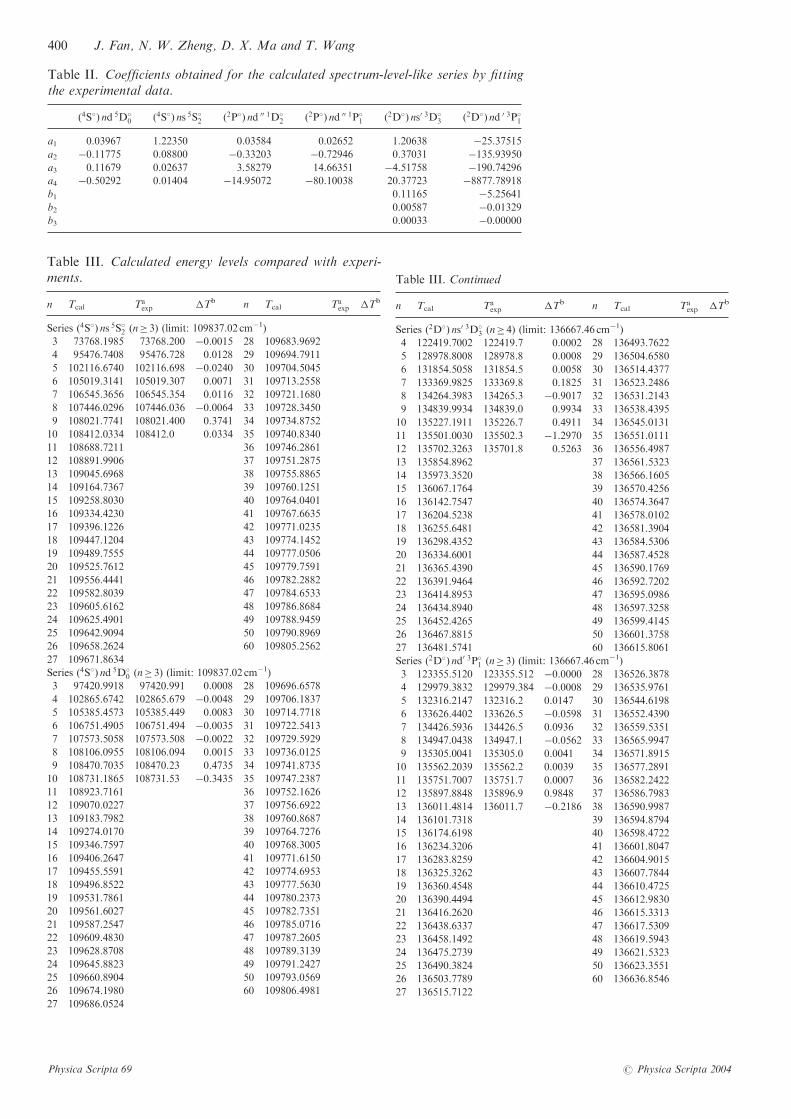
Table II. Coefficients obtained for the calculated spectrum-level-like series by fittingthe experimental data.
ð4S�Þ nd 5D�0 ð4S�Þ ns 5S�2 ð2P�Þ nd 00 1D�
2 ð2P�Þ nd 00 1P�1 ð2D�Þ ns0 3D�
3 ð2D�Þ nd 0 3P�1
a1 0.03967 1.22350 0.03584 0.02652 1.20638 �25.37515
a2 �0.11775 0.08800 �0.33203 �0.72946 0.37031 �135.93950
a3 0.11679 0.02637 3.58279 14.66351 �4.51758 �190.74296
a4 �0.50292 0.01404 �14.95072 �80.10038 20.37723 �8877.78918
b1 0.11165 �5.25641
b2 0.00587 �0.01329
b3 0.00033 �0.00000
Table III. Calculated energy levels compared with experi-ments.
n Tcal Taexp �Tb n Tcal Ta
exp �Tb
Series ð4S�Þ ns 5S�2 (n� 3) (limit: 109837.02 cm�1)
3 73768.1985 73768.200 �0.0015 28 109683.9692
4 95476.7408 95476.728 0.0128 29 109694.7911
5 102116.6740 102116.698 �0.0240 30 109704.5045
6 105019.3141 105019.307 0.0071 31 109713.2558
7 106545.3656 106545.354 0.0116 32 109721.1680
8 107446.0296 107446.036 �0.0064 33 109728.3450
9 108021.7741 108021.400 0.3741 34 109734.8752
10 108412.0334 108412.0 0.0334 35 109740.8340
11 108688.7211 36 109746.2861
12 108891.9906 37 109751.2875
13 109045.6968 38 109755.8865
14 109164.7367 39 109760.1251
15 109258.8030 40 109764.0401
16 109334.4230 41 109767.6635
17 109396.1226 42 109771.0235
18 109447.1204 43 109774.1452
19 109489.7555 44 109777.0506
20 109525.7612 45 109779.7591
21 109556.4441 46 109782.2882
22 109582.8039 47 109784.6533
23 109605.6162 48 109786.8684
24 109625.4901 49 109788.9459
25 109642.9094 50 109790.8969
26 109658.2624 60 109805.2562
27 109671.8634
Series ð4S�Þ nd 5D�0 (n� 3) (limit: 109837.02 cm�1)
3 97420.9918 97420.991 0.0008 28 109696.6578
4 102865.6742 102865.679 �0.0048 29 109706.1837
5 105385.4573 105385.449 0.0083 30 109714.7718
6 106751.4905 106751.494 �0.0035 31 109722.5413
7 107573.5058 107573.508 �0.0022 32 109729.5929
8 108106.0955 108106.094 0.0015 33 109736.0125
9 108470.7035 108470.23 0.4735 34 109741.8735
10 108731.1865 108731.53 �0.3435 35 109747.2387
11 108923.7161 36 109752.1626
12 109070.0227 37 109756.6922
13 109183.7982 38 109760.8687
14 109274.0170 39 109764.7276
15 109346.7597 40 109768.3005
16 109406.2647 41 109771.6150
17 109455.5591 42 109774.6953
18 109496.8522 43 109777.5630
19 109531.7861 44 109780.2373
20 109561.6027 45 109782.7351
21 109587.2547 46 109785.0716
22 109609.4830 47 109787.2605
23 109628.8708 48 109789.3139
24 109645.8823 49 109791.2427
25 109660.8904 50 109793.0569
26 109674.1980 60 109806.4981
27 109686.0524
Table III. Continued
n Tcal Taexp �Tb n Tcal Ta
exp �Tb
Series ð2D�Þ ns0 3D�3 (n� 4) (limit: 136667.46 cm�1)
4 122419.7002 122419.7 0.0002 28 136493.7622
5 128978.8008 128978.8 0.0008 29 136504.6580
6 131854.5058 131854.5 0.0058 30 136514.4377
7 133369.9825 133369.8 0.1825 31 136523.2486
8 134264.3983 134265.3 �0.9017 32 136531.2143
9 134839.9934 134839.0 0.9934 33 136538.4395
10 135227.1911 135226.7 0.4911 34 136545.0131
11 135501.0030 135502.3 �1.2970 35 136551.0111
12 135702.3263 135701.8 0.5263 36 136556.4987
13 135854.8962 37 136561.5323
14 135973.3520 38 136566.1605
15 136067.1764 39 136570.4256
16 136142.7547 40 136574.3647
17 136204.5238 41 136578.0102
18 136255.6481 42 136581.3904
19 136298.4352 43 136584.5306
20 136334.6001 44 136587.4528
21 136365.4390 45 136590.1769
22 136391.9464 46 136592.7202
23 136414.8953 47 136595.0986
24 136434.8940 48 136597.3258
25 136452.4265 49 136599.4145
26 136467.8815 50 136601.3758
27 136481.5741 60 136615.8061
Series ð2D�Þ nd0 3P�1 (n� 3) (limit: 136667.46 cm�1)
3 123355.5120 123355.512 �0.0000 28 136526.3878
4 129979.3832 129979.384 �0.0008 29 136535.9761
5 132316.2147 132316.2 0.0147 30 136544.6198
6 133626.4402 133626.5 �0.0598 31 136552.4390
7 134426.5936 134426.5 0.0936 32 136559.5351
8 134947.0438 134947.1 �0.0562 33 136565.9947
9 135305.0041 135305.0 0.0041 34 136571.8915
10 135562.2039 135562.2 0.0039 35 136577.2891
11 135751.7007 135751.7 0.0007 36 136582.2422
12 135897.8848 135896.9 0.9848 37 136586.7983
13 136011.4814 136011.7 �0.2186 38 136590.9987
14 136101.7318 39 136594.8794
15 136174.6198 40 136598.4722
16 136234.3206 41 136601.8047
17 136283.8259 42 136604.9015
18 136325.3262 43 136607.7844
19 136360.4548 44 136610.4725
20 136390.4494 45 136612.9830
21 136416.2620 46 136615.3313
22 136438.6337 47 136617.5309
23 136458.1492 48 136619.5943
24 136475.2739 49 136621.5323
25 136490.3824 50 136623.3551
26 136503.7789 60 136636.8546
27 136515.7122
400 J. Fan, N. W. Zheng, D. X. Ma and T. Wang
Physica Scripta 69 # Physica Scripta 2004
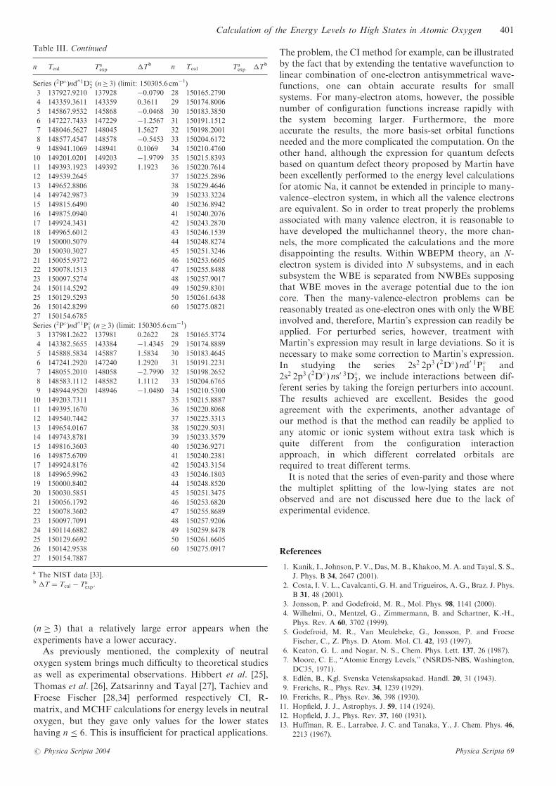
ðn � 3Þ that a relatively large error appears when the
experiments have a lower accuracy.As previously mentioned, the complexity of neutral
oxygen system brings much difficulty to theoretical studies
as well as experimental observations. Hibbert et al. [25],
Thomas et al. [26], Zatsarinny and Tayal [27], Tachiev and
Froese Fischer [28,34] performed respectively CI, R-
matrix, and MCHF calculations for energy levels in neutral
oxygen, but they gave only values for the lower states
having n � 6: This is insufficient for practical applications.
The problem, the CI method for example, can be illustratedby the fact that by extending the tentative wavefunction tolinear combination of one-electron antisymmetrical wave-functions, one can obtain accurate results for smallsystems. For many-electron atoms, however, the possiblenumber of configuration functions increase rapidly withthe system becoming larger. Furthermore, the moreaccurate the results, the more basis-set orbital functionsneeded and the more complicated the computation. On theother hand, although the expression for quantum defectsbased on quantum defect theory proposed by Martin havebeen excellently performed to the energy level calculationsfor atomic Na, it cannot be extended in principle to many-valence–electron system, in which all the valence electronsare equivalent. So in order to treat properly the problemsassociated with many valence electron, it is reasonable tohave developed the multichannel theory, the more chan-nels, the more complicated the calculations and the moredisappointing the results. Within WBEPM theory, an N-electron system is divided into N subsystems, and in eachsubsystem the WBE is separated from NWBEs supposingthat WBE moves in the average potential due to the ioncore. Then the many-valence-electron problems can bereasonably treated as one-electron ones with only the WBEinvolved and, therefore, Martin’s expression can readily beapplied. For perturbed series, however, treatment withMartin’s expression may result in large deviations. So it isnecessary to make some correction to Martin’s expression.In studying the series 2s2 2p3 ð2D�Þ nd0 1P�
1 and2s2 2p3 ð2D�Þ ns0 3D�
3; we include interactions between dif-ferent series by taking the foreign perturbers into account.The results achieved are excellent. Besides the goodagreement with the experiments, another advantage ofour method is that the method can readily be applied toany atomic or ionic system without extra task which isquite different from the configuration interactionapproach, in which different correlated orbitals arerequired to treat different terms.
It is noted that the series of even-parity and those wherethe multiplet splitting of the low-lying states are notobserved and are not discussed here due to the lack ofexperimental evidence.
References
1. Kanik, I., Johnson, P. V., Das, M. B., Khakoo, M. A. and Tayal, S. S.,
J. Phys. B 34, 2647 (2001).
2. Costa, I. V. L., Cavalcanti, G. H. and Trigueiros, A. G., Braz. J. Phys.
B 31, 48 (2001).
3. Jonsson, P. and Godefroid, M. R., Mol. Phys. 98, 1141 (2000).
4. Wilhelmi, O., Mentzel, G., Zimmermann, B. and Schartner, K.-H.,
Phys. Rev. A 60, 3702 (1999).
5. Godefroid, M. R., Van Meulebeke, G., Jonsson, P. and Froese
Fischer, C., Z. Phys. D. Atom. Mol. Cl. 42, 193 (1997).
6. Keaton, G. L. and Nogar, N. S., Chem. Phys. Lett. 137, 26 (1987).
7. Moore, C. E., ‘‘Atomic Energy Levels,’’ (NSRDS-NBS, Washington,
DC35, 1971).
8. Edlen, B., Kgl. Svenska Vetenskapsakad. Handl. 20, 31 (1943).
9. Frerichs, R., Phys. Rev. 34, 1239 (1929).
10. Frerichs, R., Phys. Rev. 36, 398 (1930).
11. Hopfield, J. J., Astrophys. J. 59, 114 (1924).
12. Hopfield, J. J., Phys. Rev. 37, 160 (1931).
13. Huffman, R. E., Larrabee, J. C. and Tanaka, Y., J. Chem. Phys. 46,
2213 (1967).
Table III. Continued
n Tcal Taexp �Tb n Tcal Ta
exp �Tb
Series ð2P�Þnd001D�2 (n� 3) (limit: 150305.6 cm�1)
3 137927.9210 137928 �0.0790 28 150165.2790
4 143359.3611 143359 0.3611 29 150174.8006
5 145867.9532 145868 �0.0468 30 150183.3850
6 147227.7433 147229 �1.2567 31 150191.1512
7 148046.5627 148045 1.5627 32 150198.2001
8 148577.4547 148578 �0.5453 33 150204.6172
9 148941.1069 148941 0.1069 34 150210.4760
10 149201.0201 149203 �1.9799 35 150215.8393
11 149393.1923 149392 1.1923 36 150220.7614
12 149539.2645 37 150225.2896
13 149652.8806 38 150229.4646
14 149742.9873 39 150233.3224
15 149815.6490 40 150236.8942
16 149875.0940 41 150240.2076
17 149924.3431 42 150243.2870
18 149965.6012 43 150246.1539
19 150000.5079 44 150248.8274
20 150030.3027 45 150251.3246
21 150055.9372 46 150253.6605
22 150078.1513 47 150255.8488
23 150097.5274 48 150257.9017
24 150114.5292 49 150259.8301
25 150129.5293 50 150261.6438
26 150142.8299 60 150275.0821
27 150154.6785
Series ð2P�Þnd001P�1 (n� 3) (limit: 150305.6 cm�1)
3 137981.2622 137981 0.2622 28 150165.3774
4 143382.5655 143384 �1.4345 29 150174.8889
5 145888.5834 145887 1.5834 30 150183.4645
6 147241.2920 147240 1.2920 31 150191.2231
7 148055.2010 148058 �2.7990 32 150198.2652
8 148583.1112 148582 1.1112 33 150204.6765
9 148944.9520 148946 �1.0480 34 150210.5300
10 149203.7311 35 150215.8887
11 149395.1670 36 150220.8068
12 149540.7442 37 150225.3313
13 149654.0167 38 150229.5031
14 149743.8781 39 150233.3579
15 149816.3603 40 150236.9271
16 149875.6709 41 150240.2381
17 149924.8176 42 150243.3154
18 149965.9962 43 150246.1803
19 150000.8402 44 150248.8520
20 150030.5851 45 150251.3475
21 150056.1792 46 150253.6820
22 150078.3602 47 150255.8689
23 150097.7091 48 150257.9206
24 150114.6882 49 150259.8478
25 150129.6692 50 150261.6605
26 150142.9538 60 150275.0917
27 150154.7887
a The NIST data [33].b �T ¼ Tcal � Ta
exp:
Calculation of the Energy Levels to High States in Atomic Oxygen 401
# Physica Scripta 2004 Physica Scripta 69
14. Huffman, R. E., Larrabee, J. C. and Tanaka, Y., J. Chem. Phys. 47,
4462 (1967).
15. Eriksson, K. B. S. and Isberg, H. B. S., Ark. Fys. 24, 549 (1963).
16. Eriksson, K. B. S. and Isberg, H. B. S., Ark. Fys. 37, 221 (1968).
17. Rudd, M. E. and Smith, K., Phys. Rev. 169, 79 (1968).
18. Edward, A. K. and Cunningham, D. L., Phys. Rev. 8, 168 (1973).
19. Mitroy, J., J. Phys. B 26, 3703 (1993).
20. Savukov, I. M. and Johnson, W. R., Phys. Rev. A 65, 042503-1 (2002).
21. Seaton, M. J., Proc. Phys. Soc. 88, 801 (1966).
22. Michel, L. and Zhilinskii, B. I., Phys. Rep. 341, 173 (2001).
23. Froese Fischer, C., ‘‘The Hartree–Fock Method for Atoms,’’ (Wiley,
New York, 1977).
24. Pradhan, A. K. and Saraph, H. E., J. Phys. B 10, 3365 (1977).
25. Hibbert, A., Biemont, E., Godefroid, M. and Vaeck, N., J. Phys. B 24,
3943 (1991).
26. Thomas, M. R. J., Bell, K. L. and Berrington, K. A., J. Phys. B 30,
4599 (1997).
27. Zatsarinny, O. and Tayal, S. S., J. Phys. B 34, 1299 (2001).
28. Tachiev, G. I. and Froese Fischer, C., Astron. Astrophys. 385, 716
(2002).
29. Zheng, N. W. et al., J. Chem. Phys. 113, 1681 (2000).
30. Zheng, N. W., Zhou, T., Yang, R. Y., Wang, T. and Ma, D. X.,
Chem. Phys. 258, 37 (2000).
31. Zheng, N. W. and Sun, Y. J., Sci. China Ser. B 43, 113 (2000).
32. Martin, W. C., J. Opt. Soc. Am. 70, 784 (1980).
33. Fuhr, J. R., Martin, W. C., Musgrove, A., Sugar, J. and Wiese, W. L.,
NIST Atomic Spectroscopic Database, Version 2.0, 1996, URL:
http://physics.nist.gov, select physical reference data.
34. Tachiev, G. and Fischer, C. F., URL: http://www.vuse.vanderbilt.
edu/�cff/mchf_collection.
402 J. Fan, N. W. Zheng, D. X. Ma and T. Wang
Physica Scripta 69 # Physica Scripta 2004