Calibration and Removal of Lateral

Chromatic Aberration in Images

John Mallon ∗ Paul F. Whelan

Vision Systems Group, Dublin City University, Dublin 9, Ireland

Abstract

This paper addresses the problem of compensating for lateral chromatic aberrationin images through colour plane realignment. Two main contributions are made: thederivation of a model for lateral chromatic aberration in images, and the subsequentclosed-form calibration of this model from a single view of a chess pattern. Theseadvances lead to a practical and accurate alternative for the compensation of lat-eral chromatic aberrations. Experimental results validate the proposed models andcalibration algorithm, while examples on real examples show how the removal oflateral chromatic aberration significantly improves the colour quality of the image.

Key words: Lateral chromatic aberration, Image warping, Camera calibration

1 Introduction

An optical instrument is required to faithfully produce a geometrically con-sistent image of a given object, where each point of the latter is imaged asa point in the image. The departure of practical optical systems from thisideal (gaussian or first order) behaviour is due to aberrations. In general is isimpossible to design a system which is free from all aberrations. This leadslens manufacturers to consider aberration compensation as an optimisationbetween different types. We are interested in chromatic aberrations that haverecently become more amplified due to the higher resolution sensors currentlyemployed in many consumer and scientific cameras. By compensating for theseaberrations as a post process in the image array, higher quality images can beproduced without recourse to expensive optics.

∗ Corresponding author. Tel.: +353 1 7005869 Fax: +353 1 7005508Email address: john.mallon@eeng.dcu.ie (John Mallon).

Preprint submitted to Elsevier Science 3 June 2005

In a colour camera’s lens, polychromatic light is split into a set of rays or wave-lengths. Whilst traversing the optical system light of different wavelengths willfollow slightly different paths. Upon reaching the image plane their misalignedrecombination introduces chromatic aberration. Chromatic Aberration (CA)can be broadly classified as Axial Chromatic Aberration (ACA) (also knownas Longitudinal CA) and Lateral Chromatic Aberration (LCA) (also known asTransverse CA). ACA arises from the longitudinal variation of focal positionwith wavelength along the optical axis. LCA is the variation of image size withwavelength or the vertical off-axis distance of a point from its prescribed point.In an image it is identified by a radially dependent misalignment of the colourplanes. Chromatic aberrations are moving out of the sub-pixel range withthe advent of high resolution arrays, giving rise to noticeable colour fringesat edges and high contrast areas. This gives the overall impression of poorquality or definition. Many consumer cameras display this aberration. For sci-entific applications, it is akin to the effects of colour shifts and blurring, thatcontravene the imaging models. We consider the digital compensation of LCAthrough image warping. There are two main aspects of digital compensationin images: determining what quantity of warp to apply, and the actual imple-mentation of the warp. Our main contribution deals with the former problem,which has currently not been addressed, by considering the modelling andmodel calibration of LCA in images.

Chromatic aberration has been predominately studied with respect to imageformation in the areas of microscopy, photogrammetry and computer vision,though recent advances in digital imaging has seen the emergence of commer-cial interest. Willson (1994) and Willson and Shafer (1991) considers an activelens control system to compensate for both LCA and ACA, by separately ad-justing three RGB filter lenses to match the colour planes. Their work showsthat chromatic aberrations can be compensated in an image by re-alignmentsof the colour channels. Boult (1992) formulates the compensation of LCA as animage warping problem. No aberration models are employed, focusing solelyon the warping problem, and correcting based only on interpolation betweencontrol points. Jackowski et al. (1997) presents a similar study on geometricand colour correction in images based on a comparison with a well definedcolour calibration chart. The models used are again surface approximations,which are far from optimal solutions, especially since only a limited numberof control points are available to estimate the surface parameters. Chromaticaberrations have been addressed by Kuzubek and Matula (2000) where analgorithm for the compensation of both LCA and ACA in fluorescence mi-croscopy is presented. This technique is not transferrable to images acquiredwith regular imaging systems.

Our proposed compensation is achieved by realigning the colour planes throughimage warping. Firstly, an LCA model is derived to precisely model the abber-ation over entire image surface. This offers a more precise and concise means

2

of extending the aberration, measured over a limited set of control points,to every pixel in the colour plane. LCA is initially measured by extractingthe intersections of a chessboard pattern on each colour plane. No special pla-narity constraints or canonical representation of the pattern is required. It canbe imaged without knowing its 3D position. Measurement errors are filteredby non-linear least square fitting of the proposed LCA model. The partialderivatives of the quadratic cost functions are given allowing the closed-formcomputation of the gradients and hessian matrices used by the optimisationalgorithms. This gives a computational advantage over numerical estimationtechniques. Detailed results clearly demonstrate the successful compensationof LCA for test images and for real scenes.

2 Geometrical Theory of Aberrations

Optically, aberrations are compensated for by adding lens elements with ap-propriate properties. Chromatic aberration is typically eliminated for two se-lected wavelengths, but only at the center and some zonal region. These lensesare known as achromatised. Lenses corrected for three different wavelengthsare known as apochromatic while superachromatic lenses are corrected forfour wavelengths. We are interested in the remaining chromatic aberrations,known as the secondary spectrum. No distinctions are made between typesof corrected lenses, as the derived models are generally applicable. Lateralchromatic aberration can be considered as the sum of two aberrations: lateralcolour distortion due to the refraction index of the lens elements and the chro-matic variation of distortion (Kingslake, 1978). We proceed by determining anappropriate model for the chromatic variation of distortion in the image plane.

2.1 Chromatic variation of distortion

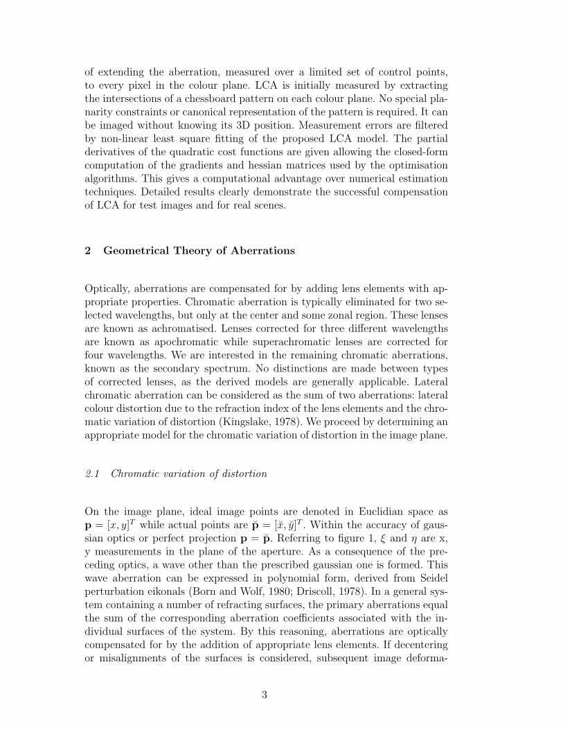
On the image plane, ideal image points are denoted in Euclidian space asp = [x, y]T while actual points are p = [x, y]T . Within the accuracy of gaus-sian optics or perfect projection p = p. Referring to figure 1, ξ and η are x,y measurements in the plane of the aperture. As a consequence of the pre-ceding optics, a wave other than the prescribed gaussian one is formed. Thiswave aberration can be expressed in polynomial form, derived from Seidelperturbation eikonals (Born and Wolf, 1980; Driscoll, 1978). In a general sys-tem containing a number of refracting surfaces, the primary aberrations equalthe sum of the corresponding aberration coefficients associated with the in-dividual surfaces of the system. By this reasoning, aberrations are opticallycompensated for by the addition of appropriate lens elements. If decenteringor misalignments of the surfaces is considered, subsequent image deforma-

3

Fig. 1. General optical setup.

tion may be approximated by perturbing the intermediately formed image byx1 → x1 + λ and y1 → y1 + µ. Considering the distortion component of thewave aberration equation, the corresponding wave aberration for the combinedsurfaces to a fourth order approximation is:

φ = k1r2κ2 + λk1(ξ(3x

2 + y2) + 2ηxy) + µk1(η(3y2u + x2

u) + 2ξxuyu),

where r2 = x2 + y2 and κ2 = xξ + yη. The constant k1 = E1 + ...En is the sumof the individual lens contributions. The combined decentering effects of mul-tiple lens elements also sums in a linear fashion. The altered wavefront is theroot of all aberrations formed on the image by distorting the ray projections.These ray aberrations are evaluated as the shift from the predicted gaussiancoordinates by ∆x = x − x = ∂φ

∂ξand ∆y = y − y = ∂φ

∂η(Born and Wolf,

1980). Evaluating this using the fourth order approximation of φ, results inthe combined cartesian model of distortion.

CD(p,k)x = k1xr2 + p1(3x2 + y2) + 2p2xy

CD(p,k)y = k1yr2 + 2p1xy + p2(3y2 + x2), (1)

where k = [k1, p1, p2]T are the parameters, p1 = λk1 and p2 = µk1. In this

function the radial component is represented by k1, while the distortions in-troduced by decentering correspond to p1 and p2. This decentering model isequivalent to that of Conrady (1919) as promoted by Brown (1966), foundthrough exact ray tracing techniques. In many lenses a secondary chromaticspectrum exhibits a decentering form. Its inclusion leads to more a generalmore general model and improved modelling accuracy. This is investigatedfurther in section 4.

4

2.2 Lateral colour distortion

In addition to the chromatic variation of distortion there is an additionallateral colour distortion that is due to the refraction index variation of thelens elements. The refraction index is quite linear within the visible spectrumKingslake (1978), resulting in the addition of an extra first order term thatdoes not appear in the chromatic distortion equation. Deviations from linearbehaviour are naturally accounted for in the chromatic distortion equation.Thus, the combined LCA for a specific frequency (g), can thus be modelled asa function of another frequency (f) by the addition of the chromatic variationof distortion and the lateral colour distortion as:

Cg(pf , cg)x = c1xf + c2xfr2f + c3(3x

2f + y2

f ) + 2c4xfyf

Cg(pf , cg)y = c1yf + c2yfr2f + 2c3xfyf + c4(3y

2f + x2

f ), (2)

where cf = [c1, c2, c3, c4]T is the parameter vector.

3 Model Calibration

Lateral chromatic aberration is modelled for a specific frequency accordingto equation 2. The actual secondary spectrum is difficult to exactly quantify,but manifests itself by misalignments in the colour planes as demonstratedby Willson (1994). These planes typically match the RGB filters of a typicalcolour sensor, though any other colour representations can be used, as themethods are general. If one colour plane is taken as a reference, chromaticaberration can be compensated for by realigned the other planes with thisreference. This reference colour is chosen as the Green (G) channel, as it isit is midway within the visible spectrum and generally exhibits a low averagemagnitude in the secondary spectrum.

3.1 Measuring lateral chromatic aberrations

Chromatic aberration has previously been measured by Kuzubek and Matula(2000) using florescent dyed beads. These are then imaged in 3D, when theircentroids are estimated. From these centroids the LCA and ACA are measured.This approach is only suited to fluorescent microcopy, but the measured LCAexhibits a similar profile to the results obtained using our approach. WillsonWillson (1994), measures chromatic aberration by comparing the location ofedges detected on three colour planes. In this paper lateral chromatic aber-ration is measured by detecting the intersections of a chessboard pattern for

5

each of the colour planes. These are automatically extracted by a two stageprocess of initial detection and sub-pixel refinement.

Initial estimates for the location of chessboard type intersection are obtainedusing standard corner detectors such as those described in Lucchese and Mi-tra (2002); Jain et al. (1995). For real situations where additional corners aredetected, a further refinement step is necessary to remove false hits. A smallN ×N region of interest, Ψ, centered on the candidate corner is first thresh-olded using the mean gray level of Ψ. A symmetry measure tΨ can then becalculated as:

tΨ =N∑

v=0

N∑

u=0

O(u, v), where O(u, v) =

a ifΨ(u, v) = Ψ(N − u, N − v)

Ψ(u, v) 6= Ψ(u,N − v),

b otherwise.

where (u, v) are the pixel coordinates, a and b are positive and negative con-stants. We obtain good performance using a = 6 and b = −1 with N = 9.High values of the symmetry measure tΨ indicate the corner is situated on achessboard intersection.

For each colour plane the initial corner estimate is refined using a small N×Nregion of interest Ψ. A bilinear quadratic function is linearly fit to the intensityprofile:

mins‖s1u

2 + s2uv + s3v2 + s4u + s5v + s6 −Ψ(u, v)‖2.

The intersection point or saddle point is derived from this surface as theintersection of the two lines 2s1u + s2v + s4 = 0 and s2u + 2s3v + s5 = 0. Nospecial data ordering is necessary as comparisons are not made to externalcoordinate system. The accuracy of this detection method is examined insection 4.

3.2 Chromatic parameter estimation

The pattern intersection points are represented in pixel coordinates as mf =(uf , vf )

T for a certain colour plane f . Given the image width and heightas w and h, the intersection coordinates are normalised by scaling mf =(uf , vf )

T /s = (uf , vf )T , where s = (w + h)/2. The normalised optical axis or

center point of the apparent abberation, (xf , yf )T , also needs to be estimated,

as it generally does not lie at the center of the image. It is initially estimatedas xf = w/2s and yf = h/2s. For some cases an aspect difference (a) alsoneeds to be estimated. Fully scaled points on a certain colour plane are thusdenoted by:

pf = (xf , yf )T = (auf + xf , vf + yf )

T ,

6

where f denotes the colour plane, in this case either red (r), blue (b) or green(g).

The lateral misalignments between the red and green planes is modelled as afunction of the green plane, following equation 2 as:

Cr(pg, cr)x

Cr(pg, cr)y

=

c1xg + c2xgr2g + c3(3x

2g + y2

g) + 2c4xgyg

c1yg + c2ygr2g + 2c3xgyg + c4(3y

2g + x2

g)

, (3)

and similarly for the difference between the blue and green planes. For eachdetected intersection point, two equations are formed. It is sufficient to followthese equations with respect to the red/green planes only:

e(θr) =

ex(θr)

ey(θr)

=

ug + Cr(pg, cr)x − ur

vg + Cr(pg, cr)y − vr

, (4)

where the parameter vector to be estimated is θr = (x, y, a, c1, c2, c3, c4).

This function is minimised using a quadratic cost function j(θ) = eT (θ)Qe(θ),where Q is the estimated covariance, (assumed an identity matrix in this case).Performing a first order expansion of the error e around the last iterativeestimate θk, results in a Gauss-Newton scheme that can be iterated utilisingmany robust least square techniques Golub and Loan (1996):

θk+1 = θk − λ

(∂eT (θk)

∂θ

∂e(θk)

∂θT

)−1∂eT (θk)

∂θe(θk), (5)

where λ ≤ 1 ensures a decrease in cost at each step. The partial derivativesused in the closed-form calculation are given as:

∂e(θk)

∂θT=

∂ex(θk)∂θT

∂ey(θk)∂θT

=

∂ex(θk)∂x

, ∂ex(θk)∂y

, ∂ex(θk)∂a

, xg, xgr2g , 3x

2g + y2

g , 2xgyg

∂ey(θk)∂x

, ∂ey(θk)∂y

, ∂ey(θk)∂a

, yg, ygr2g , 2xgyg, 3y

2g + x2

g

,

with

∂ex(θk)∂x

∂ey(θk)∂x

=

c1 + c2(3x2g + y2

g) + 6c3xg + 2c4yg

2c2xgyg + 2c3yg + 2c4xg

,

∂ex(θk)∂y

∂ey(θk)∂y

=

2c2xgyg + 2c3yg + 2c4xg

c1 + c2(x2g + 3y2

g) + 2c3xg + 6c4yg

,

∂ex(θk)∂a

∂ey(θk)∂a

=

c1ug + 3c2x2gug + 6c3xgug + 2c4ugyg

2c3ygug + 2c4xgug

.

7

Equation 5 is iterated until θk+1−θk falls below a preset threshold. The param-eter vector can be simply initialised as θ0

r = (−w/2s,−h/2s, 1, 0, 0, 0, 0), andthe estimation algorithm shows good convergence behaviour, as investigatedin section 4. In analysis, due to the performed normalisation, no improve-ment was achieved using constant variance/maximum likelihood or bias freeestimation schemes.

4 Experiments

Chessboard patterns and real images are used to measure the effects of LCAcompensation. Three different commercial digital cameras are used to cap-ture the test images. The pattern used for calibration is shown in figure 2. Nocanonical coordinates are required for calibration, hence no precise constraintsare needed on the planarity or precision of the pattern. A second lower densitychessboard pattern (test image), shown in figure 2, is used for independent val-idation of the proposed LCA model and the resulting realignments. Algorithmconvergence is examined for both colour channel alignments. Finally, shots ofan outdoor scene are used to demonstrate the typical improvement in imagequality following LCA compensation.

Fig. 2. Chessboard patterns used for calibration (calib image) and testing (testimage) taken with cam 1, see tables 1 and 2.

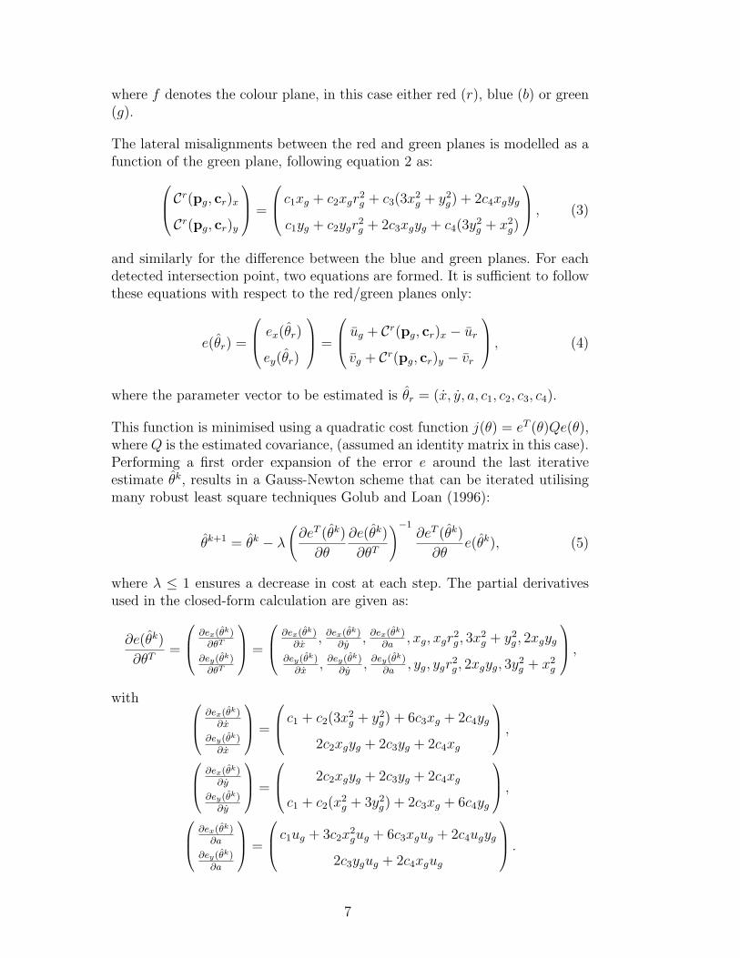
The intersections of the chessboard patterns are firstly determined for eachcolour plane. The typical sub-pixel detection accuracy of the techniques out-lined in section 3.1 are shown in figure 3 for the three cameras used in theexperiments. The colour plane misalignments before calibration for the twochessboard patterns are presented in table 1. Following calibration, the knownLCA models are used to warp the colour planes so as to register the red andblue colour planes with the green channel. The Euclidean registration residu-

8

0.2 0.4 0.6 0.80

0.05

0.1

0.15

0.2

0.25

0.3 h

(ε)

Cam 1: µε = 0.1459 σε = 0.083979

Euclidean error (pixels)0.2 0.4 0.6 0.8 1

0

0.02

0.04

0.06

0.08

0.1

0.12

0.14

h(ε

)

Cam 3: µε = 0.27163 σε = 0.13057

Euclidean error (pixels)0.2 0.4 0.6 0.8 1

0

0.05

0.1

0.15

h(ε

)

Cam 2: µε = 0.26765σε = 0.14915

Euclidean error (pixels)

Fig. 3. Histogram of sub-pixel detection errors for three different cameras withtheir fitting with Rayleigh PDF. Errors are estimated using multiple shots of thecalibration pattern.

Table 1Colour plane misalignments (in pixels) before calibration in mean (standard de-viation) format for three different cameras. R/G and B/G are the red and bluemisalignments with reference to the green channel.

Cam 1 Cam 2 Cam 3

Calib R/G 0.5707 (0.2113) 0.5496 (0.2308) 1.1834 (0.4125)

Image B/G 0.4110 (0.2635) 0.7374 (0.6361) 0.5665 (0.3848)

Test R/G 0.5355 (0.2225) 0.5413 (0.2035) 0.9729 (0.2866)

Image B/G 0.4877 (0.2925) 1.1630 (0.8971) 0.8378 (0.7956)

als remaining following this re-registration are presented in table 2, showinga significant decrease in misalignments. These residuals are of a similar mag-nitude to the sub-pixel detection accuracy, thus validating both the proposedLCA model and the effectiveness of the proposed calibration algorithm.

As described in section 2, some lenses exhibit a significant tangential LCAcomponent. The results presented in table 3 show the Euclidean registra-tion residuals following compensation based on a model without tangentialelements. The increase in these residuals compared with those of the full cali-bration model indicated that although radial chromatic aberration is predom-inant, there is a varying element of tangential abberation based on the lensemployed. The inclusion of tangential elements in the LCA description gives amore general and accurate model of lateral chromatic aberration in an image.

Full details of the colour plane misalignments before and after calibrationare presented for one example (Cam 1) from table 1 and 2. Figure 4 showsthe distribution of colour plane misalignments before and after compensationfor LCA for the calibration pattern in figure 2. The corresponding Euclideanvector representation of these misalignments for the test image, before and

9

Table 2Colour plane misalignments (in pixels) following calibration and colour plane warp-ing in mean (standard deviation) format for three different cameras.

Cam 1 Cam 2 Cam 3

Calib R/G 0.1202 (0.0636) 0.1401 (0.0733) 0.1846 (0.0722)

Image B/G 0.1376 (0.0734) 0.1658 (0.0947) 0.1543 (0.0925)

Test R/G 0.1788 (0.1062) 0.1625 (0.0784) 0.2044 (0.1149)

Image B/G 0.1879 (0.1110) 0.3092 (0.2146) 0.3202 (0.2419)

Table 3Colour plane misalignments (in pixels) following calibration and warping using amodel without tangential elements in mean (standard deviation) format for threedifferent cameras.

Cam 1 Cam 2 Cam 3

Calib R/G 0.1828 (0.0904) 0.1615 (0.0858) 0.2196 (0.1208)

Image B/G 0.2131 (0.1117) 0.1805 (0.1087) 0.1507 (0.0754)

Test R/G 0.1864 (0.1110) 0.2022 (0.1019) 0.1886 (0.1449)

Image B/G 0.2071 (0.1334) 0.3670 (0.3070) 0.3761 (0.3029)

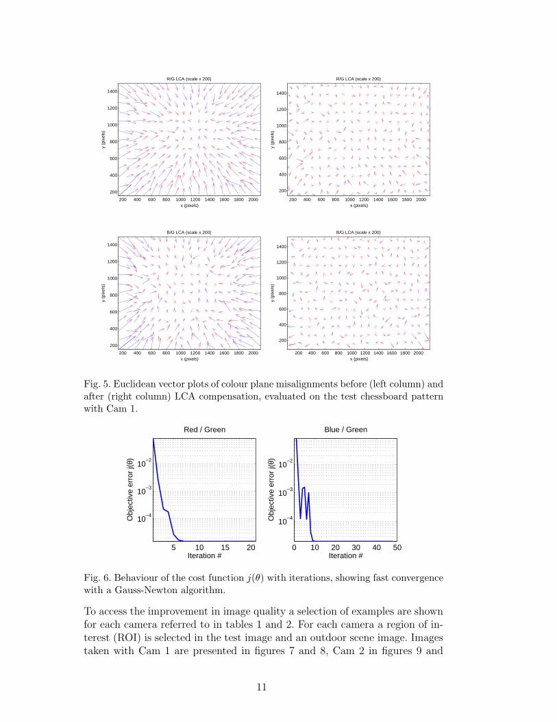
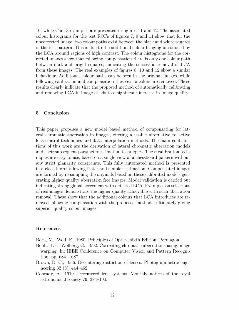
after compensation, are illustrated in figure 5. These show that the remainingmisalignments are random in nature (with magnitude similar to the detectionnoise), indicating the successful modelling and compensation of LCA. Theconvergence of the proposed algorithm using data from Cam 1 is shown infigure 6, showing fast convergence, usually after 10 iterations.

0.2 0.4 0.6 0.8 10

0.02

0.04

0.06

0.08

h(ε

)

Red green LCA

0.2 0.4 0.6 0.8 1 1.20

0.05

0.1

h(ε

)

Blue green LCA

Euclidean error (pixels)

µε = 0.5707σε = 0.2113

µε = 0.411σε = 0.2635

0.05 0.1 0.15 0.2 0.25 0.3 0.350

0.1

0.2

0.3

0.4

h(ε

)

Red green LCA

0.05 0.1 0.15 0.2 0.25 0.3 0.35 0.40

0.1

0.2

0.3

h(ε

)

Blue green LCA

Euclidean error (pixels)

µε = 0.1202σε = 0.06361

µε = 0.1376σε = 0.07341

Fig. 4. Histograms of Euclidean misalignments computed for chessboard intersec-tions on the calibration image with Cam 1. Left column shows the R/G and B/Gdifferences before compensation, while the right column shows those detected fol-lowing calibration with fitted Rayleigh PDF’s.

10

200 400 600 800 1000 1200 1400 1600 1800 2000

200

400

600

800

1000

1200

1400

x (pixels)

y (

pixe

ls)

R/G LCA (scale x 200)

200 400 600 800 1000 1200 1400 1600 1800 2000

200

400

600

800

1000

1200

1400

x (pixels)

y (

pixe

ls)

R/G LCA (scale x 200)

200 400 600 800 1000 1200 1400 1600 1800 2000

200

400

600

800

1000

1200

1400

x (pixels)

y (

pixe

ls)

B/G LCA (scale x 200)

200 400 600 800 1000 1200 1400 1600 1800 2000

200

400

600

800

1000

1200

1400

x (pixels)

y (

pixe

ls)

B/G LCA (scale x 200)

Fig. 5. Euclidean vector plots of colour plane misalignments before (left column) andafter (right column) LCA compensation, evaluated on the test chessboard patternwith Cam 1.

0 10 20 30 40 50

10−4

10−3

10−2

Blue / Green

Iteration #

Obj

ectiv

e er

ror

j(θ)

5 10 15 20

10−4

10−3

10−2

Red / Green

Iteration #

Obj

ectiv

e er

ror

j(θ)

Fig. 6. Behaviour of the cost function j(θ) with iterations, showing fast convergencewith a Gauss-Newton algorithm.

To access the improvement in image quality a selection of examples are shownfor each camera referred to in tables 1 and 2. For each camera a region of in-terest (ROI) is selected in the test image and an outdoor scene image. Imagestaken with Cam 1 are presented in figures 7 and 8, Cam 2 in figures 9 and

11

10, while Cam 3 examples are presented in figures 11 and 12. The associatedcolour histograms for the test ROI’s of figures 7, 9 and 11 show that for theuncorrected image, two colour paths exist between the black and white squaresof the test pattern. This is due to the additional colour fringing introduced bythe LCA around regions of high contrast. The colour histograms for the cor-rected images show that following compensation there is only one colour pathbetween dark and bright squares, indicating the successful removal of LCAfrom these images. The real examples of figures 8, 10 and 12 show a similarbehaviour. Additional colour paths can be seen in the original images, whilefollowing calibration and compensation these extra colors are removed. Theseresults clearly indicate that the proposed method of automatically calibratingand removing LCA in images leads to a significant increase in image quality.

5 Conclusion

This paper proposes a new model based method of compensating for lat-eral chromatic aberration in images, offering a usable alternative to activelens control techniques and data interpolation methods. The main contribu-tions of this work are the derivation of lateral chromatic aberration modelsand their subsequent parameter estimation techniques. These calibration tech-niques are easy to use, based on a single view of a chessboard pattern withoutany strict planarity constraints. This fully automated method is presentedin a closed-form allowing faster and simpler estimation. Compensated imagesare formed by re-sampling the originals based on these calibrated models gen-erating higher quality aberration free images. Model validation is carried outindicating strong global agreement with detected LCA. Examples on selectionsof real images demonstrate the higher quality achievable with such aberrationremoval. These show that the additional colours that LCA introduces are re-moved following compensation with the proposed methods, ultimately givingsuperior quality colour images.

References

Born, M., Wolf, E., 1980. Principles of Optics, sixth Edition. Permagon.Boult, T.E.; Wolberg, G., 1992. Correcting chromatic aberrations using image

warping. In: IEEE Conference on Computer Vision and Pattern Recogni-tion. pp. 684 – 687.

Brown, D. C., 1966. Decentering distortion of lenses. Photogrammetric engi-neering 32 (3), 444–462.

Conrady, A., 1919. Decentered lens systems. Monthly notices of the royalastronomical society 79, 384–190.

12

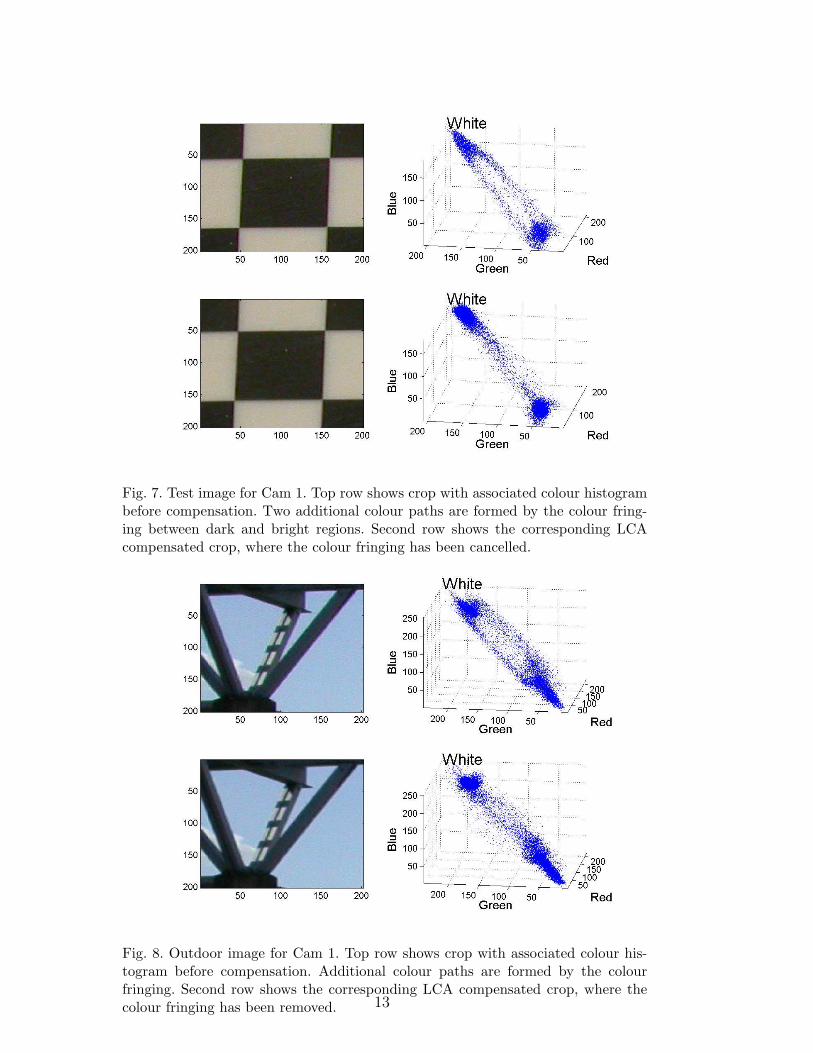
Fig. 7. Test image for Cam 1. Top row shows crop with associated colour histogrambefore compensation. Two additional colour paths are formed by the colour fring-ing between dark and bright regions. Second row shows the corresponding LCAcompensated crop, where the colour fringing has been cancelled.

Fig. 8. Outdoor image for Cam 1. Top row shows crop with associated colour his-togram before compensation. Additional colour paths are formed by the colourfringing. Second row shows the corresponding LCA compensated crop, where thecolour fringing has been removed. 13

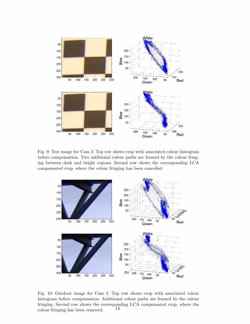
Fig. 9. Test image for Cam 2. Top row shows crop with associated colour histogrambefore compensation. Two additional colour paths are formed by the colour fring-ing between dark and bright regions. Second row shows the corresponding LCAcompensated crop, where the colour fringing has been cancelled.

Fig. 10. Outdoor image for Cam 2. Top row shows crop with associated colourhistogram before compensation. Additional colour paths are formed by the colourfringing. Second row shows the corresponding LCA compensated crop, where thecolour fringing has been removed. 14

Fig. 11. Test image for Cam 3. Top row shows crop with associated colour histogrambefore compensation. Two additional colour paths are formed by the colour fring-ing between dark and bright regions. Second row shows the corresponding LCAcompensated crop, where the colour fringing has been cancelled.

Fig. 12. Outdoor image for Cam 3. Top row shows crop with associated colourhistogram before compensation. Additional colour paths are formed by the colourfringing. Second row shows the corresponding LCA compensated crop, where thecolour fringing has been removed. 15

Driscoll, W. G., 1978. Handbook of optics. McGraw Hill.Golub, G. H., Loan, C. F. V., 1996. Matrix Computation, 3rd Edition. Johns

Hopkins University Press.Jackowski, M., Goshtasby, A., Bines, S., Roseman, D., Yu, C., 1997. Correcting

the geometry and color of digital images. IEEE Transactions on PatternAnalysis and Machine Intelligence 19 (10), 1152–1158.

Jain, R., Kasturi, R., Schunck, B. G., 1995. Machine vision. McGraw-Hill.Kingslake, R., 1978. Lens Design fundamentals. academic press.Kuzubek, M., Matula, P., 2000. An efficient algorithm for measurement and

correction of chromatic aberrations in fluorescence microscopy. Journal ofMicroscopy 200 (3), 206–217.

Lucchese, L., Mitra, S. K., 2002. Using saddle points for subpixel feature de-tection in camera calibration targets. In: Asia-Pacific Conference on Circuitsand Systems. Vol. 2. pp. 191 – 195.

Willson, R., 1994. Modeling and calibration of automated zoom lenses. Ph.D.thesis, Carnegie Mellon University.

Willson, R. G., Shafer, S. A., 1991. Active lens control for high precisioncomputer imaging. In: IEEE International conference on robotics and au-tomation. pp. 2063–2070.

16