Embed Size (px)
Citation preview
Calibration of Speed-Density Relationships for Freeways in Aimsun
RAFFAELE MAURO Department of Mechanical and Structural Engineering
Università degli Studi di Trento, Italy Via Mesiano, 77 - 38123 Trento
ITALY [email protected]
ORAZIO GIUFFRÈ
Department of Civil, Environmental, Aerospace, Materials Engineering Università degli Studi di Palermo, Italy
Viale delle Scienze, 90128 Palermo ITALY
ANNA GRANÀ Department of Civil, Environmental, Aerospace, Materials Engineering
Università degli Studi di Palermo, Italy Viale delle Scienze, 90128 Palermo
ITALY [email protected]
SANDRO CHIAPPONE
Department of Civil, Environmental, Aerospace, Materials Engineering Università degli Studi di Palermo, Italy
Viale delle Scienze, 90128 Palermo ITALY
Abstract: - The first application of a calibration methodology which uses speed-density relationships in the microsimulation calibration process is described in this article. Traffic patterns were implemented developing speed-density relationships for empirical and simulated data. For empirical relationships reference was made to traffic data observed at A22 Freeway (Italy). Aimsun microscopic traffic simulator software was then used to obtain analogous relationships for a test freeway segment under uncongested traffic conditions. Thus on field conditions were reproduced varying some calibration parameters until a good matching between field and simulation was achieved. The closeness between empirical data and simulation outputs was assessed through a statistical approach which included hypothesis testing and confidence intervals. Key-Words: - road, traffic, density, speed, freeway, microsimulation, calibration.
1 Introduction Road traffic microsimulation models have in recent years become widely accepted as useful tools that perform highly detailed analysis to identify interventions and evaluate the effects of proposed solutions before their implementation in the real world. Traffic microsimulation consists in the dynamic and stochastic modeling of individual
vehicle movements within a system of transportation facilities. Each vehicle is moved through the road network basing on the physical characteristics of the vehicle, the fundamental rules of motion and rules of driver behavior (i.e. car following, lane changing and gap acceptance rules).
Despite the representation of individual drivers determines a high level of complexity in the
Recent Advances in Civil Engineering and Mechanics
ISBN: 978-960-474-403-9 176
modeling process, traffic microsimulation models allow to simulate traffic behavior with high accuracy. However, in order to gain a high level of accuracy, substantial amounts of roadway geometry, traffic control, traffic pattern, and driver behavior data are required. Moreover, traffic microsimulation models contain many adjustable parameters, inherent to characteristics of travelers, vehicles and roads, and the relevant adjustments have to be performed from the calibration stage [1]. Before the microsimulation model is used as prediction tool of road traffic performances, it is essential to verify that the right parameters are modified to correctly represent the situation under examination.
Repeated iterations in the calibration process may be necessary to assure that the model reproduces real-world traffic conditions reasonably well; after changing and adjusting some model parameters, model outputs have to be compared with a set of empirical data until the model outputs are similar to empirical data at a predetermined level of agreement [2]. However, the achievement of calibration targets can be influenced by the simplification of which microsimulation models are not free. Since each microsimulation model cannot include all the variables affecting real-world traffic conditions, each microsimulation software contain a set of user-adjustable parameters; moreover, the relevant adjustments can vary for each software package. On this regard, technical literature proposes some studies focusing on which parameters have to be adjusted by the analyst during the model calibration process to match locally observed conditions [3][4][5][6][7]. Lots of methodologies for calibrating microsimulation models has been recently proposed in the literature, but there have been no attempts to identify general calibration principles based on their collective experience (see for further details [1]). However, the process of checking to what extent the built model correctly represents real-world traffic conditions needs two independent data sets be used: the first set of data for the calibration of the model parameters and the second set for the running of the calibrated model so that the model output data can be compared to the second set of system output data [8]. The comparison part is referred to as the validation of the calibrated model.
In this paper a calibration methodology which uses speed-density relationships in the microsimulation calibration process is presented. As is well known, speed-density relationships represent
the traffic flow phenomenon in a wide range of operational conditions and well summarize the information which can be collected on field or by the microsimulation model. Differently from calibration procedures proposed by the technical literature, closeness between empirical data and simulation outputs is achieved through a statistical approach which included hypothesis testing and confidence intervals. An uncongested freeway segment was selected as case study. Based on field observations at the A22 Brenner Freeway, Italy, statistical regressions between the traffic flow variables were developed. Analogous relationships were obtained using the Aimsun microscopic traffic simulator software, reproducing field conditions and varying some selected parameters until a good matching between field and simulation was achieved.
2 Calibration methodologies for microsimulation models Some procedures for performing a calibration use a single measure [4]; other procedures use more than one measure by performing a sequence of calibration sub-processes, in which a separate group of parameters is calibrated using a different traffic measure [5]. For instance, Dowling et al. [9] proposed that microsimulation calibration should be performed in three basic steps: calibrate capacity at key bottlenecks; calibrate traffic volumes; calibrate system performance. Calibration of the model to capacity has as target to obtain the matching of the model outputs as close as possible to the field-measured capacities. However, loss of information can derive by defining capacity as a single numerical value, despite it clearly has to be represented by a distribution of capacity values; for an introduction to the stochastic nature of capacity see [10]. Moreover, if the capacity calibration process is based on a single numerical value, matching the means of capacity distribution does not necessarily match the other important properties of a distribution, nor even other traffic parameters characterizing capacity as speed or density [7].
It should be noted that capacity information can be derived from speed-density, speed-flow and flow-density relationships; they also provide information on free-flow, congested, and queue discharge regions which cannot be deduced from one numerical value or a distribution of capacities. Thus, basing on speed-flow, speed-density, or flow-density relationships, a calibration procedure could replicate the range of traffic behavior in its entirety.
Recent Advances in Civil Engineering and Mechanics
ISBN: 978-960-474-403-9 177
However, for model calibration only a portion of one of the three graphs mentioned above instead of the entire graph could be used [7]. The amount of information available in fitting empirical/simulated data is very important; thus more information can be derived from speed-flow, speed-density, or flow-density graphs. By using a higher number of parameters in the calibration process, a better fine-tuned simulation model can be obtained. The calibration of speed-flow, speed-density, or flow-density graphs can represent one step in microsimulation calibration, then followed by route-choice calibration and system performance calibration. However, the use of the fundamental relationships of traffic flow in the microsimulation calibration process are extremely limited. It is known that the concept of replicating field speed-flow relationships and using them to demonstrate closeness of field and simulated data was also applied [11], whereas the ability of a simulation model to replicate speed-flow graphs from real-world freeways was demonstrated [12]. An objective function based on minimizing the dissimilarity between speed-flow graphs was developed and reported in [7]; the dissimilarity of two graphs by calculating the amount of area that is not covered by the other was also measured. Moreover, considering that the information derived from the field and simulation was not a complete speed-flow graph, the comparison was only made over the space occupied by the field graph.
3 The traffic flow diagram for the A22 Brenner Freeway, Italy Based on data collected at different observation sections on the A22 Brenner Freeway, Italy, the speed-flow-density relationships for a traffic flow of cars only were modeled; these relationships were developed for the right lane, the passing lane and the roadway [13]. A criterion for predicting the reliability of A22 Freeway traffic flow by observing speed stochastic processes was also proposed [14].
First the relationship between speed and density was searched. V=V(D) is a monotonically decreasing function, implying a mathematical relation simpler than the flow-density and speed-flow relationships; this relationship, indeed, is not difficult to observe in the real world, while the effects of speed and density on flow are not quite as apparent. Starting from the speed-density models suggested by literature (i.e. single-regime models, two-regime models, multi-regime models), May model [15] was chosen to interpret the available
data at the observed sections. According to [15], the relationship between speed and density is as follows:
⋅−⋅=
2
5.0expc
FF D
DVV (1)
where: VFF = the free flow speed; Dc = the critical density, namely the density to
which is associated the reaching of the capacity C. Converting eq. 1 into linear form, the logarithmic
transformation was used:
( ) ( ) 22cD2
1-lnln DVV FF ⋅
⋅= (2)
By using the speed-flow-density relationship, Q=DV, it was possible to obtain the flow Q as follows:
⋅−⋅⋅=
2
5.0expc
FF D
DDVQ (3)
Thus V = V(Q) and Q = Q(D) relationships were obtained; for their specification values of VFF and Dc were estimated. Traffic flow models were calibrated for the right lane, the passing lane and the roadway at the sections under examination. Basing on the scatter plot (D2; lnV), according to equation 2, a least squares estimation was performed; VFF and Dc were calculated for all observation sections [13]. By using equations 1 and 3, the speed-flow-density relationships were specified for each observation section; the values of capacity C and speed Vc (i.e. the speed corresponding to C) were also estimated. Then the homologous determinations of VFF and Dc at the observation sections were averaged; using the obtained values of VFF and Dc, the speed-flow-density relationships for each lane and the roadway for A22 Freeway were developed.
Table 1 shows the averaged values of the parameters for relationships between the fundamental variables of traffic flow for the A22 Freeway. In Table 2 the values of VFF, Dc, C and Vc at S. Michele observation section (southbound) are shown; this section was used in the calibration of the microsimulation model.
4 Calibration of Model Parameters In order to produce a micro-simulation model faithful to traffic conditions experienced on A22 Freeway, traffic patterns and driver behavior were replicated by using Aimsun micro-simulator. Aimsun is traffic modeling software having sufficient user-adjustable parameters available to control car-following, lane changing, gap generation
Recent Advances in Civil Engineering and Mechanics
ISBN: 978-960-474-403-9 178
and acceptance behavior, and to model freeway traffic flow. In addition to this, a calibration procedure was proposed to faithfully produce existing traffic conditions (see section 5).
Table 1. The parameters of speed-flow-density relationships for the A22 Freeway, Italy
Table 2. The parameters of speed-flow-density relationships for S. Michele section (southbound)
It is well known that in the Aimsun micro-
simulator, during a vehicle's journey along the road network, its position is updated according to two driver behavior models named “car following” and “lane changing” [2]. The car-following model in Aimsun is an evolution of the empirical model proposed by Gipps [16][17]. Indeed, the implementation of the car-following model proposed by Gipps in Aimsun includes not only the vehicle and its leader but also the influence of certain vehicles driving slower in the adjacent lane on the vehicle driving along a section. The lane change model in Aimsun can also be considered as a further evolution of the Gipps lane change model [17]; lane change is modeled as a decision process analyzing the necessity of the lane change, the desirability of the lane change, and the feasibility conditions for the lane change that are also depending on the location of the vehicle on the road network [2]. For an overview of the car following and lane-changing parameters the reader is referred to [2].
Considering that the model calibration is critical as it has to provide some degree of assurance that the model will be able to reproduce local traffic
conditions and driver behavior, a proper calibration of parameters was undertaken rather than using the default values. The fine tuning process involved the iterative changing of some parameters and simulation runs until the model outputs were as close as possible to empirical data. Thus some default values for calibration parameters were changed, basing on experience gained so far and judgment. Numerous iteration were carried out, manually adjusting various combinations of these parameters to improve the performance of the system; iterations were stopped when a good match between empirical and simulated data was achieved according to the criterion explained in the next section 5. Table 3 shows the selected parameters and their default/used values.
Table 3. Calibration Parameters
In the calibration process the desired speeds (i.e.
the maximum speed, in km/h, that a certain type of vehicle can travel at any point in the network) were also adjusted. For instance, in Aimsun a car vehicle type is characterized by a mean desired speed of 110 km/h and a deviation of 10 km/h; desired speed for this vehicle type is sampled from a truncated Normal distribution (110, 10). According to empirical data and what reported in [18], the desired speeds for right lane were assumed lower than those for the passing lane. Trial runs allowed to note that the desired speed was sensitive to flow rate, tending to decrease as flow rate values became consistent. Thus, adjustments for the mean desired speeds (used here as a proxy variable) were differentiated by traffic demand values, for each lane and the roadway, as follows: − from 500 to 1500 [pcu/h], the values 110 km/h
and 140 km/h were assumed for the right lane and passing lane, respectively, whereas the value 125 km/h was assumed for the roadway;
lane/lanes of travel
VFF Dc C VC
right lane 106.95 23.65 1534 64.86
passing lane 130.28 25.09 1983 79.02
roadway 117.45 48.56 3459 71.23
lane/lanes of travel
VFF Dc C VC
right lane 105.00 24.36 1551 64.00
passing lane 131.50 24.67 1967 80.00
roadway 118.20 48.35 3467 72.00
Parameter definition Default Used
minimum headway [s]
the time between the leader and the follower vehicle
2.10 1.70
minimum distance between
vehicles [m]
the distance that a vehicle keeps
between itself and the preceding vehicle when
stopped
1.10 1.00
reaction time [s]
the time a driver takes for reacting to speed changes in the preceding
vehicle
0.70 0.80
Recent Advances in Civil Engineering and Mechanics
ISBN: 978-960-474-403-9 179
− for 2000 [pcu/h], the values 100 km/h and 140 km/h were assumed for the right lane and passing lane, respectively, whereas the value 115 km/h was assumed for the roadway;
− for 2500 [pcu/h], the values 95 km/h and 140 km/h were assumed for the right lane and passing lane, respectively, whereas the value 115 km/h was assumed for the roadway;
− for values > 3000 [pcu/h], the values 90 km/h and 130 km/h were assumed for the right lane and passing lane, respectively, whereas the value 115 km/h was assumed for the roadway. A 2 km long freeway segment was used in the
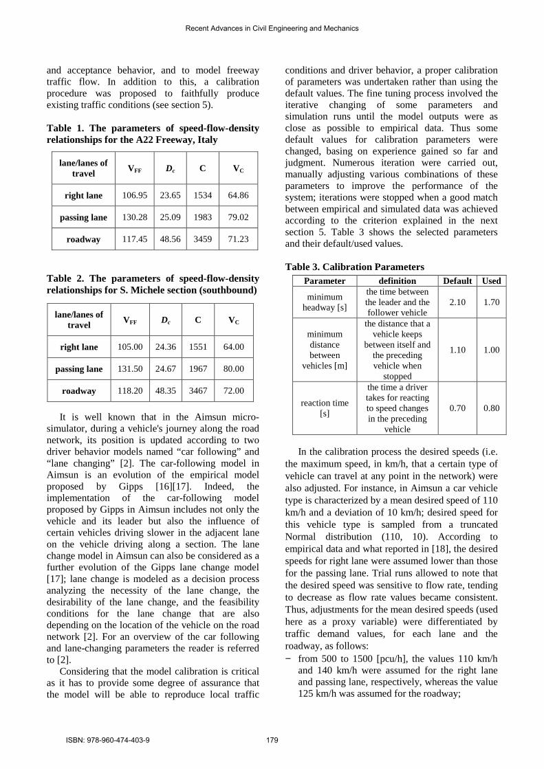
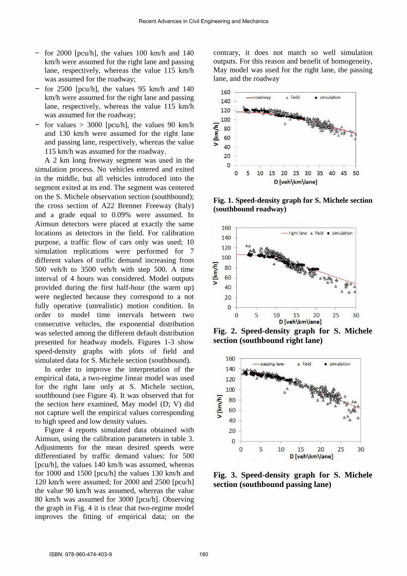
simulation process. No vehicles entered and exited in the middle, but all vehicles introduced into the segment exited at its end. The segment was centered on the S. Michele observation section (southbound); the cross section of A22 Brenner Freeway (Italy) and a grade equal to 0.09% were assumed. In Aimsun detectors were placed at exactly the same locations as detectors in the field. For calibration purpose, a traffic flow of cars only was used; 10 simulation replications were performed for 7 different values of traffic demand increasing from 500 veh/h to 3500 veh/h with step 500. A time interval of 4 hours was considered. Model outputs provided during the first half-hour (the warm up) were neglected because they correspond to a not fully operative (unrealistic) motion condition. In order to model time intervals between two consecutive vehicles, the exponential distribution was selected among the different default distribution presented for headway models. Figures 1-3 show speed-density graphs with plots of field and simulated data for S. Michele section (southbound).
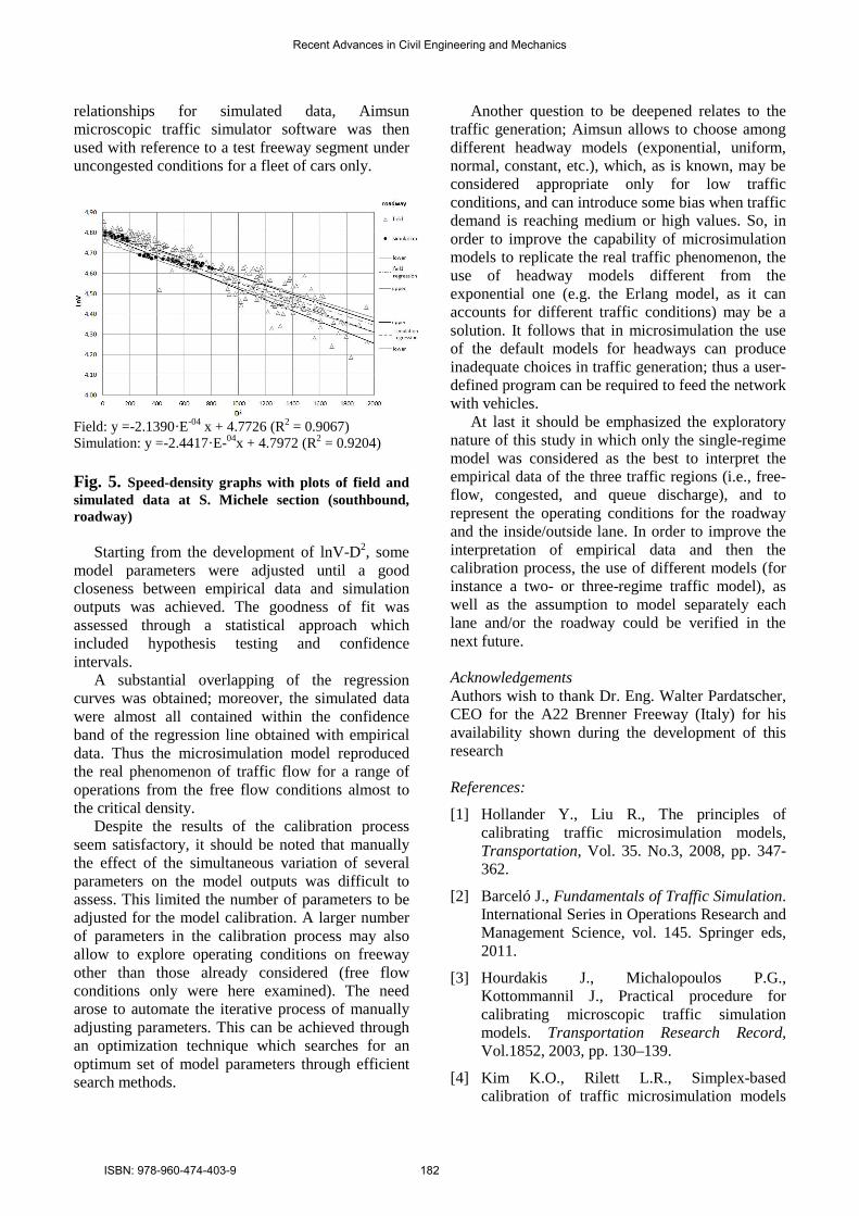
In order to improve the interpretation of the empirical data, a two-regime linear model was used for the right lane only at S. Michele section, southbound (see Figure 4). It was observed that for the section here examined, May model (D; V) did not capture well the empirical values corresponding to high speed and low density values.
Figure 4 reports simulated data obtained with Aimsun, using the calibration parameters in table 3. Adjustments for the mean desired speeds were differentiated by traffic demand values: for 500 [pcu/h], the values 140 km/h was assumed, whereas for 1000 and 1500 [pcu/h] the values 130 km/h and 120 km/h were assumed; for 2000 and 2500 [pcu/h] the value 90 km/h was assumed, whereas the value 80 km/h was assumed for 3000 [pcu/h]. Observing the graph in Fig. 4 it is clear that two-regime model improves the fitting of empirical data; on the
contrary, it does not match so well simulation outputs. For this reason and benefit of homogeneity, May model was used for the right lane, the passing lane, and the roadway
Fig. 1. Speed-density graph for S. Michele section (southbound roadway)
Fig. 2. Speed-density graph for S. Michele section (southbound right lane)
Fig. 3. Speed-density graph for S. Michele section (southbound passing lane)
Recent Advances in Civil Engineering and Mechanics
ISBN: 978-960-474-403-9 180
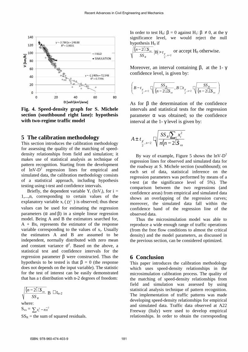
Fig. 4. Speed-density graph for S. Michele section (southbound right lane): hypothesis with two-regime traffic model
5 The calibration methodology This section introduces the calibration methodology for assessing the quality of the matching of speed-density relationships from field and simulation; it makes use of statistical analysis as technique of pattern recognition. Starting from the development of lnV-D2 regression lines for empirical and simulated data, the calibration methodology consists of a statistical approach, including hypothesis testing using t-test and confidence intervals.
Briefly, the dependent variable Yi (lnVi), for i = 1,...,n, corresponding to certain values of the explanatory variable xi ( 2
iD ) is observed; thus these values can be used for estimating the regression parameters (α and β) in a simple linear regression model. Being A and B the estimators searched for, A + Bxi represents the estimator of the response variable corresponding to the values of xi. Usually the estimators A and B are assumed to be independent, normally distributed with zero mean and constant variance σ2. Based on the above, a statistical test and confidence intervals for the regression parameter β were constructed. Thus the hypothesis to be tested is that β = 0 (the response does not depends on the input variable). The statistic for the test of interest can be easily demonstrated that has a t distribution with n-2 degrees of freedom:
( ) B
2
R
xx
SS
Sn ⋅− ∼ tn-2
where: Sxx = ∑ −
i i xnx22
SSR = the sum of squared residuals.
In order to test H0: β = 0 against H1: β ≠ 0, at the γ significance level, we would reject the null hypothesis H0 if
( )2 ,
2
B 2
−>⋅−
nR
xx tSS
Snγ
or accept H0 otherwise.
Moreover, an interval containing β, at the 1- γ confidence level, is given by:
( ) ( )
⋅−⋅+
⋅−⋅−
−−xx
R
nxx
R
n Sn
SStB
Sn
SStB
2,
2
2 , 2
2 , 2
γγ
As for β the determination of the confidence intervals and statistical tests for the regression parameter α was obtained; so the confidence interval at the 1- γ level is given by:
( ) 2
2
2 , 2 xx
i iR
n Snn
xSStA
−⋅
⋅± ∑−γ
By way of example, Figure 5 shows the lnV-D2
regression lines for observed and simulated data for the roadway at S. Michele section (southbound); on each set of data, statistical inference on the regression parameters was performed by means of a t-test (at the significance level of 5%). The comparison between the two regressions (and confidence areas) from empirical and simulated data shows an overlapping of the regression curves; moreover, the simulated data fall within the confidence band of the regression line of the observed data.
Thus the microsimulation model was able to reproduce a wide enough range of traffic operations (from the free flow conditions to almost the critical density) and the model parameters, as discussed in the previous section, can be considered optimized.
6 Conclusion This paper introduces the calibration methodology which uses speed-density relationships in the microsimulation calibration process. The quality of the matching of speed-density relationships from field and simulation was assessed by using statistical analysis technique of pattern recognition. The implementation of traffic patterns was made developing speed-density relationships for empirical and simulated data. Traffic data observed at A22 Freeway (Italy) were used to develop empirical relationships. In order to obtain the corresponding
Recent Advances in Civil Engineering and Mechanics
ISBN: 978-960-474-403-9 181
relationships for simulated data, Aimsun microscopic traffic simulator software was then used with reference to a test freeway segment under uncongested conditions for a fleet of cars only.
Field: y =-2.1390·E-04 x + 4.7726 (R2 = 0.9067) Simulation: y =-2.4417·E-04x + 4.7972 (R2 = 0.9204) Fig. 5. Speed-density graphs with plots of field and simulated data at S. Michele section (southbound, roadway)
Starting from the development of lnV-D2, some model parameters were adjusted until a good closeness between empirical data and simulation outputs was achieved. The goodness of fit was assessed through a statistical approach which included hypothesis testing and confidence intervals.
A substantial overlapping of the regression curves was obtained; moreover, the simulated data were almost all contained within the confidence band of the regression line obtained with empirical data. Thus the microsimulation model reproduced the real phenomenon of traffic flow for a range of operations from the free flow conditions almost to the critical density.
Despite the results of the calibration process seem satisfactory, it should be noted that manually the effect of the simultaneous variation of several parameters on the model outputs was difficult to assess. This limited the number of parameters to be adjusted for the model calibration. A larger number of parameters in the calibration process may also allow to explore operating conditions on freeway other than those already considered (free flow conditions only were here examined). The need arose to automate the iterative process of manually adjusting parameters. This can be achieved through an optimization technique which searches for an optimum set of model parameters through efficient search methods.
Another question to be deepened relates to the traffic generation; Aimsun allows to choose among different headway models (exponential, uniform, normal, constant, etc.), which, as is known, may be considered appropriate only for low traffic conditions, and can introduce some bias when traffic demand is reaching medium or high values. So, in order to improve the capability of microsimulation models to replicate the real traffic phenomenon, the use of headway models different from the exponential one (e.g. the Erlang model, as it can accounts for different traffic conditions) may be a solution. It follows that in microsimulation the use of the default models for headways can produce inadequate choices in traffic generation; thus a user-defined program can be required to feed the network with vehicles.
At last it should be emphasized the exploratory nature of this study in which only the single-regime model was considered as the best to interpret the empirical data of the three traffic regions (i.e., free-flow, congested, and queue discharge), and to represent the operating conditions for the roadway and the inside/outside lane. In order to improve the interpretation of empirical data and then the calibration process, the use of different models (for instance a two- or three-regime traffic model), as well as the assumption to model separately each lane and/or the roadway could be verified in the next future. Acknowledgements Authors wish to thank Dr. Eng. Walter Pardatscher, CEO for the A22 Brenner Freeway (Italy) for his availability shown during the development of this research References:
[1] Hollander Y., Liu R., The principles of calibrating traffic microsimulation models, Transportation, Vol. 35. No.3, 2008, pp. 347-362.
[2] Barceló J., Fundamentals of Traffic Simulation. International Series in Operations Research and Management Science, vol. 145. Springer eds, 2011.
[3] Hourdakis J., Michalopoulos P.G., Kottommannil J., Practical procedure for calibrating microscopic traffic simulation models. Transportation Research Record, Vol.1852, 2003, pp. 130–139.
[4] Kim K.O., Rilett L.R., Simplex-based calibration of traffic microsimulation models
Recent Advances in Civil Engineering and Mechanics
ISBN: 978-960-474-403-9 182
with intelligent transportation systems data. Transportation Research Record, Vol. 1855, 2003, pp. 80–89.
[5] Dowling R., Skabardonis A., Halkias J., McHale G., Zammit G., 2004a. Guidelines for Calibration of Microsimulation Models: Framework and Applications. Transportation Research Record, Vol. 1876, 2004, pp. 1–9.
[6] Toledo T., Koutsopoulos H.N., Davol A., Ben-Akiva M.E., Burghout W., Andreasson I., Johansson T., Lundin C., Calibration and validation of microscopic traffic simulation tools. Stockholm case study. Transportation Research Record, Vol. 1831,2003, pp. 65–75.
[7] Menneni S., Sun C., Vortisch P., Microsimulation Calibration Using Speed-Flow Relationships. Transportation Research Record, Vol. 2088,2009, pp. 1-9.
[8] Toledo T., Koutsopoulos H.N., Statistical Validation of Traffic Simulation Models. Transportation Research Record, Vol.1876, 2004, pp. 142–150.
[9] Dowling R., Skabardonis A., Vassili A., Traffic Analysis Toolbox Volume III: Guidelines for Applying Traffic Microsimulation Software. Report No. FHWA-HRT-04-040. 2004b.
[10] Brilon W., Geistefeldt J., Zurlinden H., Implementing the Concept of Reliability for Highway Capacity Analysis. 87th TRB Annual Meeting, 2007, Washington, DC, USA.
[11] Wiedemann R., Modelling of RTI-Elements on Multi-Lane Roads. Advanced Telematics in Road Transport, Vol. II, 1991, pp. 1001–1019.
[12] Fellendorf M., Vortisch P., Validation of the Microscopic Traffic Flow Model VISSIM in Different Real-World Situations. 80th TRB Annual Meeting, 2001, Washington, DC, USA.
[13] Mauro R., Analisi di traffico, elaborazione di modelli e sistemi per la stima dell’affidabilità per l’Autostrada A22, Italia [Traffic analysis, development of models and systems for estimating reliability on the A22 Freeway, Italy] . Technical report, Part I,II, III - Autostrada del Brennero, Trento, Italy (in Italian), 2003; 2005; 2007.
[14] Mauro R., Giuffrè O., Granà A., Speed Stochastic Processes and Freeway Reliability Estimation: Evidence from the A22 Freeway, Italy. Journal of Transportation Engineering, Vol. 139, No. 12, 2013, 1244–1256.
[15] May A.D., Traffic Flow Fundamentals. Prentice Hall, Inc. USA, 1990.
[16] Gipps P.G., A behavioral car-following model for computer simulation. Transportation Research Record, Vol. 15-B, No.2, 1981, pp 105–111.
[17] Gipps P.G., A model for the structure of lane-changing decisions. Transportation Research Record, Vol. 20-B, No.5, 1986, pp. 403–414.
[18] Uddin M.S.; Ardekani S., An Observational Study of Lane Changing on Basic Freeway Segment. 81st TRB Annual Meeting, Washington, DC, USA, 2002.
Recent Advances in Civil Engineering and Mechanics
ISBN: 978-960-474-403-9 183