California Dreamin’ of Higher Wages · California Dreamin’ of Higher Wages William E. Even Raymond E. Glos Professor of Economics | Miami University David A. Macpherson E.M. Stevens

California Dreamin’ of Higher Wages

William E. EvenRaymond E. Glos Professor of Economics | Miami University

David A. MacphersonE.M. Stevens Professor of Economics | Trinity University

Evaluating the Golden State’s 30-Year Minimum Wage Experiment

DECEMBER 2017

The Employment Policies Institute (EPI) is a non-profit research organiza-

tion dedicated to studying public policy issues surrounding employment

growth. In particular, EPI focuses on issues that affect entry-level employ-

ment. Among other issues, EPI research has quantified the impact of new labor

costs on job creation, explored the connection between entry-level employment

and welfare reform, and analyzed the demographic distribution of mandated bene-

fits. EPI sponsors nonpartisan research which is conducted by independent econo-

mists at major universities around the country.

DECEMBER 2017

EPIONLINE.ORG

California Dreamin’ of Higher WagesEvaluating the Golden State’s 30-Year Minimum Wage Experiment

William E. EvenRaymond E. Glos Professor of Economics | Miami University

David A. MacphersonE.M. Stevens Professor of Economics | Trinity University

2 | EMPLOYMENT POLICIES INSTITUTE

EXECUTIVE SUMMARYIn recent decades, California has pursued mini-mum wage levels about the federal standard. By 2022, the state will have the first statewide mini-mum wage of $15.00 per hour.

The Golden State’s minimum wage experience thus offers a unique opportunity for researchers to examine the longer-term economic effects of high minimum wages.

In this new study, Dr. David Macpherson of Trinity University and Dr. William Even of Miami Univer-sity measure the empirical effects of minimum wage increases in California from 1990 to the present, and estimate the impact of California’s current minimum wage law.

Even and Macpherson adopt a novel approach to measure minimum wage impacts, examining the impacts of a rising minimum wage on pri-vate sector employment across county-industry pairs between 24 counties and 15 industries in California. Over nearly three decades of data, the economists attempt to isolate the employment impact of a rising minimum wage from broader trends in California’s economy—for instance, the substantial decline in manufacturing employ-ment in Los Angeles County.

In total, the authors employ 24 unique variations of their original model to ensure as fair a treat-ment of the evidence as reasonably possible.

Their findings are stark: The economists’ pre-ferred model shows that past minimum wage

increases in California have caused a measur-able decrease in employment among affected employees. Specifically, they find that a 10% increase in the minimum wage would cause a nearly five-percent reduction in employment in an industry where one-half of workers earn wag-es close to the minimum. In an industry with an average share of lower-wage workers, their find-ings imply that each 10% increase in California’s minimum wage has reduced employment for af-fected employees by two percent.

The authors apply these estimates to the state’s forthcoming $15 minimum wage. By 2022, ap-proximately 400,000 jobs would be lost as a consequence. (This estimate is conservative, as it measures the impact of California’s state min-imum wage but does not account for job loss in counties that had insufficient data.) Industries with the greatest number of affected employees are most severely affected by job loss, according to Even and Macpherson; nearly half of the ob-served job loss occurs in foodservice and retail industries.

Whether the real-time response of an economy will mitigate or exacerbate the effects of raising the minimum wage is an open question. What is not in dispute, based on this study, is that Cali-fornia’s rising minimum wage has depressed em-ployment opportunities in the most heavily-im-pacted industries. The conclusions should give pause to states or localities interested in emulat-ing California’s wage experiment.

CALIFORNIA DREAMIN’ OF HIGHER WAGES | 3

INTRODUCTIONSince 1980, the state of California has passed sev-eral minimum wage laws that increased the min-imum wage beyond the federal level. One might argue that a higher minimum wage is justified in California because of its relatively high cost of liv-ing compared the typical state. On the other hand, one might be concerned about whether the high-er minimum wage in California causes job loss for low skilled workers, and whether the effects differ in the cities where the cost of living and wages are relatively high as compared to rural areas or less expensive cities.

This study examines the effect of California’s state minimum wage laws since 1990. It tests for an effect of a higher minimum wage by examin-ing whether a minimum wage increase is associ-ated with a slowdown in employment growth in county-industry pairs with a greater share of low wage workers. Relying on several different empir-ical models, our analysis finds that post minimum wage increases that occurred in California have caused a reduction in employment. Our study also simulates the effect of the current law that is scheduled to raise the minimum wage to $15.00 by 2022. The simulations suggest that the $15.00 minimum could cause a loss of about 400,000 jobs in California1.

The job loss is not spread evenly. Slightly more than one-half of the job loss is projected to be in two industries: accommodation and food services, and retail trade. While the most populated coun-ties of California are expected to incur the largest employment loss in terms of the number of work-ers, the smaller counties generally experience a larger percentage point loss in employment due to the lower wages and the greater number of workers that would be affected by the minimum wage hike.

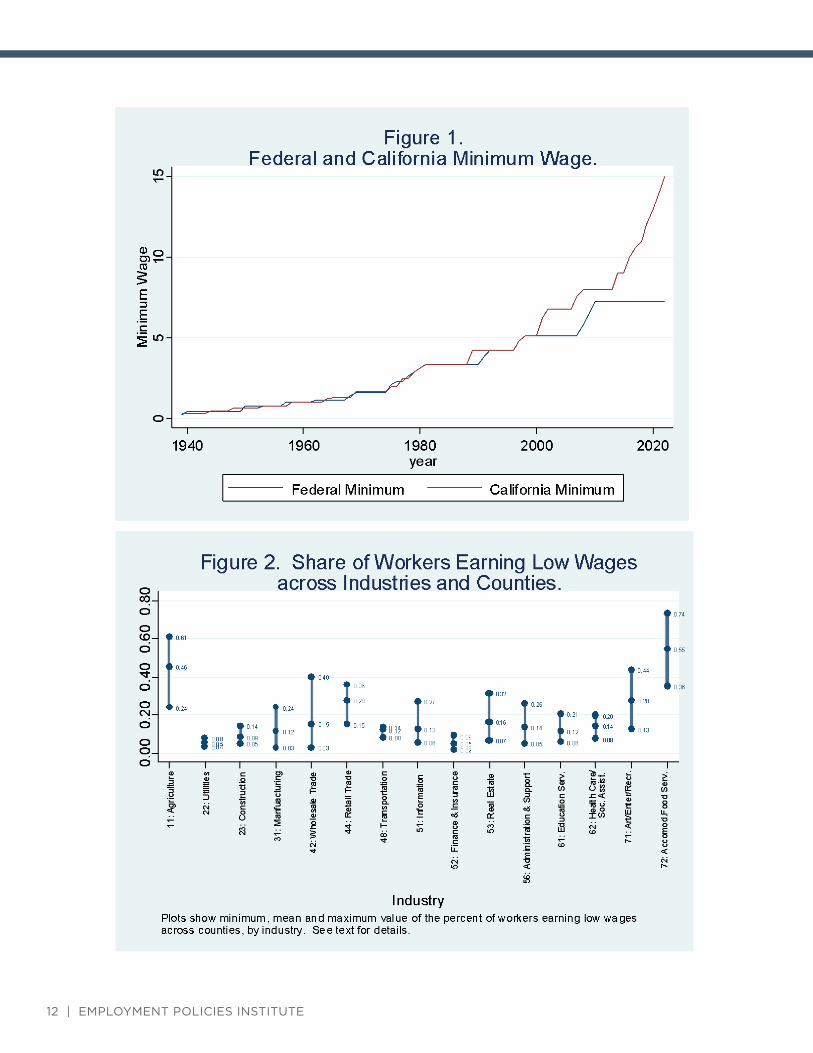
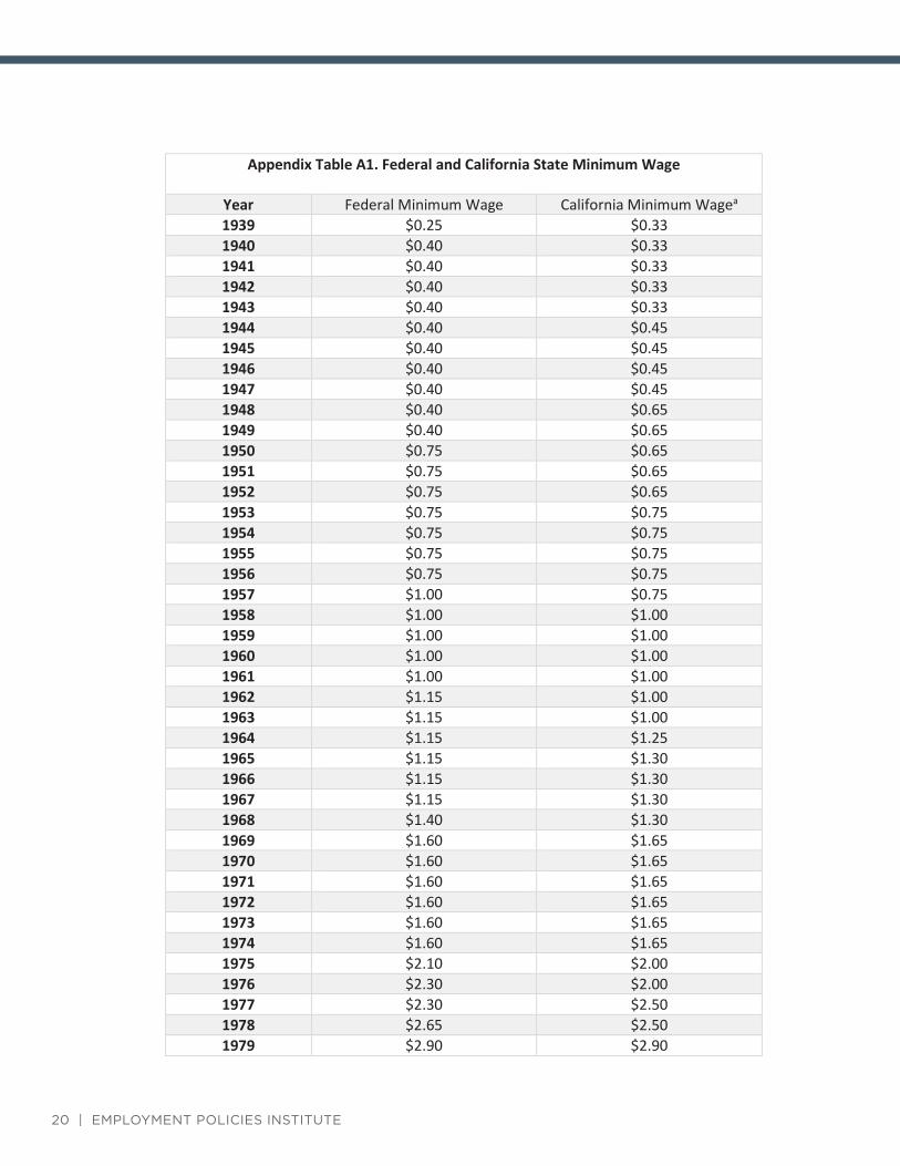
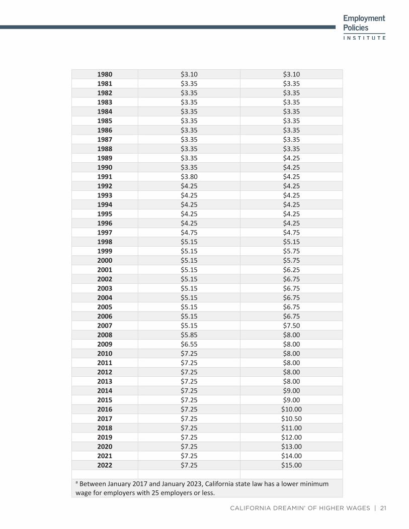
MINIMUM WAGE HISTORY IN THE STATE OF CALIFORNIAFigure 1 provides a comparison of the federal and California minimum wage from 1990 through 2022. For 2018 through 2022, the minimum wag-es are based on legislation passed as of July 2017. The figure makes it clear that, beginning in 2001, California began a practice of increasing its mini-mum wage at a faster rate than mandated by fed-eral law. In 2001, the California minimum exceed-ed the federal minimum by $1.10 ($6.25 versus $5.15). The gap between the California and fed-eral minimum fluctuated since 2000 as both the state and federal minimum wages increased. As of 2017, California’s $10.50 minimum is among the highest statewide minimum in the country. More-over, under current law, California’s will increase its minimum wage to $15.00 by 2022 while the federal minimum is scheduled to remain at $7.25. If current laws remain in effect, this will lead to the largest gap between a state and federal minimum wage in the history of the U.S.

This study uses the California experience between 1994 and 2016 as a way to gauge the effect of the upcoming increases in the minimum wage on employment in California. While numerous stud-ies have examined the effect of minimum wage hikes on employment [see Neumark and Washer (2008)l; Congressional Budget Office (2014); and Neumark (2015) for a review of such studies], our study is unique in two ways. First, we focus en-tirely on the employment experience in California. The labor market in California differs from many other states because of the mixture of rural and urban counties, the mixture of industries, and the large differences in the cost of living and wages across these counties. Second, unlike much of the recent research that estimates the effect of minimum wage hikes by comparing employment trends across states that differ in terms of their minimum wage laws, we compare employment growth across county-industry pairs (CIPs) with-

1This estimate does not include the job loss in rural areas not included in our analysis.2 Several cities will have a $15 minimum wage prior to 2022, including Seattle, Los Angeles, San Francisco, New York City, and Wash-ington D.C.

in California to determine the effects. That is, we obtain a measure of the extent to which the min-imum wage should be binding in each CIP and test whether a minimum wage increase slows em-ployment growth most where the minimum wage binds the most.

THE DATATo test for differences in employment growth across CIPs, we use data from the Quarterly Cen-sus of Employment and Wages (QCEW) between 1990 and the second quarter of 2016. The QCEW data provides a quarterly count of employment and payroll reported by employers and covers 98 percent of U.S. jobs. The quarterly counts are available at the county, state, and national levels by industry. The data provide a complete tabula-tion of employment and total payroll for workers covered by either state or federal unemployment insurance programs. We restrict our analysis to private sector employers. Self-employed workers are not included in the data.

Our analysis of employment trends uses employ-ment by county for each 2 digit NAICS indus-try. We convert to annual employment measures by averaging across the quarterly employment counts to remove seasonality in the data. Since employment counts are masked for confidential-ity reasons when a given CIP has a low level of employment, we restrict our analysis to those CIPs that have employment reported in every quarter between 1990 and 2016.

For our analysis, we need a measure of how much the minimum wage binds in each CIP. The QCEW reports total payroll and the number of workers. Given this aggregate level of data and the lack of information on hours worked, the QCEW earnings data is not suitable for estimating the share of workers earning a wage close to the minimum. To obtain an estimate, we use the Outgoing Rotation

Groups of the Current Population Survey between 1996 and 20163. We estimate the percentage of workers in an industry that we define as “low wage workers” – which we define as anyone earning no more than between $.25 below the state minimum (in nominal dollars) and $1 above (in 1990 dollars).

Unfortunately, the CPS identifies only 31 of the 58 California counties and our analysis is thus re-stricted to this subset. To help improve the accu-racy of our wage estimate for a CIP, we drop any county that contains a city minimum wage law that causes its minimum wage to differ from the California state minimum wage and simultaneous-ly differ within the county4. While San Francisco has a minimum wage above the state level, this is a county-wide minimum wage so we include it in our analysis.

To assure that our wage estimates for a CIP are reasonably accurate, we exclude any CIP with less than 200 observations on wages in the CPS sam-ple. The sample also excludes any CIP that has in-complete employment data over the sample peri-od. These tend to be relatively small CIPs because the QCEW masks employment counts when there is a concern that disclosing the CIP employment count could reveal too much information about a specific establishment. We also exclude any coun-ty when the total employment for the included in-dustries covered less than one-half of private sec-tor employment in the county in 2016. Finally, we eliminate any CIP that shows more than a 25 per-cent change in employment between years. Such changes are clear outliers in the data and may re-flect changes in reporting behavior by a firm that has multiple establishments5.

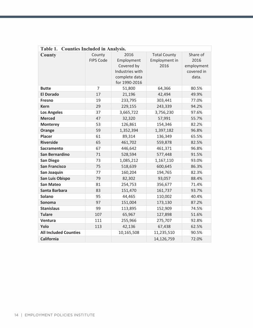
Table 1 provides a list of the 24 counties that fit our requirements for inclusion along with the em-ployment level in each county. In total, there 11.2 million private sector workers in the 24 counties included. 90.5 percent of the private sector em-ployment in these 24 counties is covered in our sample, and it represents 72.0 percent of state-

3 We choose a starting date of 1996 for the CPS data because the counties identified in the CPS changed in 1996. We also had to map census codes for industry to match those in the QCEW and account for the fact that industry codes changed in both the CPS and QCEW over time.

4 This restriction results in Alameda, Contra Costa, and Santa Clara counties being dropped from the sample. The largest cities in these counties are Oakland, Concord, and San Jose, respectively.


wide private sector employment. While a large share of private sector employment is included in our sample, the restrictions admittedly result in small rural counties being underrepresented since data is more likely to be suppressed when em-ployment counts are low.

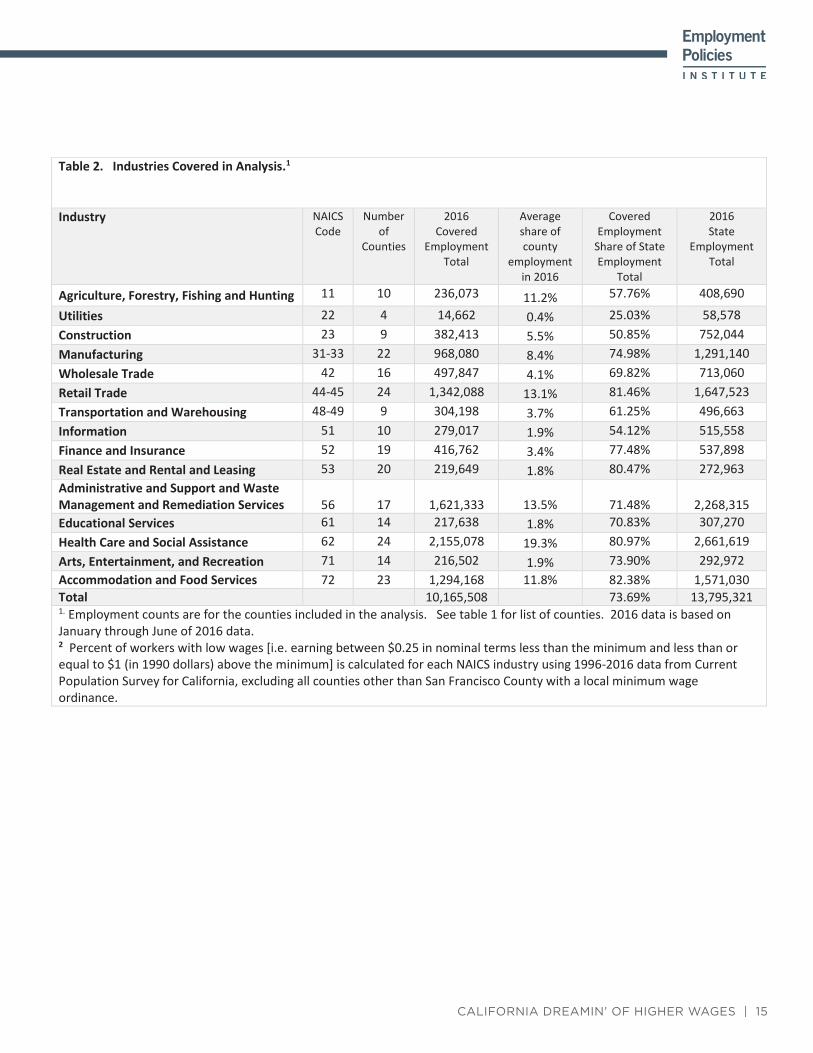
Table 2 provides a list of the industries that we in-clude in the sample, the number of counties with adequate employment data for each industry, and the share of state-wide employment covered in our sample. The industries that are included in our sample employed 13.8 million workers in California in 2016 Our sample includes 73.7 percent of state-wide employment in these industries. The indus-tries with the highest share of state-wide employ-ment covered by our sample are those that have sufficient data to be covered by a large number of counties.

Figure 2 describes the variation in the share of workers earning low wages across CIPs. For each industry, the figure shows the minimum, max-imum, and average share of workers with low wages across counties. The 2 industries with the largest share of low wage workers are accommo-dation and food services (55 percent low wage) and agriculture, forestry, fishing and hunting (46 percent low wage). At the other extreme, the two industries with the lowest share of workers earn-ing low wages are utilities, and finance and insur-ance (both at 5 percent).

Within a given industry, there is a substantial vari-ation in the share of workers earning low wages across counties. For example, in accommodation and food services, the share ranges from 36 to 74 percent; in agriculture, the range is from 24 to 61 percent. As a result, the extent to which a mini-mum wage increase binds will vary substantially across both counties and industries.

EMPIRICAL APPROACHOur empirical approach for determining the effect of California minimum wage hikes uses regres-sion analysis to determine whether increases in the state minimum wages cause employment to rise more slowly in CIPs where the minimum wage binds more and affects more workers.

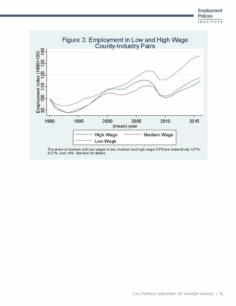
To provide some context for the analysis, Figure 3 provides an illustration of employment trends for low, medium, and high wage CIPs. The split between the three wage levels is based upon the percentage of workers earning low wages. The CIPs in the bottom quartile of workers earning low wages (i.e. less than 8 percent earning low wag-es) are classified as high wage CIPs. Those in the top quartile of the distribution—with more than 27 percent of workers earning low wages—are classi-fied as low wage CIPs. The CIPs that are neither in the top or bottom quartile earning low wages are classified as medium wage industries.

The employment measure is an index set to 100 in 1990. Based on the information provided, employ-ment since 1990 grew by 37, 18, and 15 percent in low, medium and high wage CIPS since 1990. This evidence alone might lead one to erroneously conclude that California’s minimum wage increas-es have not slowed (and perhaps increased) em-ployment in low wage industries. Such a conclu-sion would be inappropriate since other economic factors may have caused the employment trends to differ across high, medium and low wage CIPs. There may be economic forces at work (such as import competition, technical change [Baily and Bosworth (2014); Autor and Dorn (2013)] that cause industries to grow at different rates. For example, increased import competition and tech-nological change have led to declines in U.S. man-ufacturing employment [Autor et al. (2013, 2015); Pierce and Schott (2016)]. In our data, manufac-turing is either a high or medium wage industry in all counties. Consequently, import competition

5 The Bureau of Labor Statistics points out that, in the QCEW, large month-to-month changes in employment could reflect changes in employer reporting practices at the beginning of a new calendar year. For example, an employer might have multiple locations in the state may report as a single corporation. In a subsequent reporting period, the company may change their method of reporting leading to a large change in employment. This issue is discussed on the BLS website at https://www.bls.gov/cew/cewfaq.htm#Q11.


and/or technological change may have caused employment growth to slow in high and medium wage industries. A failure to account for such in-dustry specific trends would lead to a misinterpre-tation of the data.

Another important factor that needs to be con-sidered in comparing employment growth across CIPs is that some counties are growing at a faster rate than others. More rapid growth in low wage counties (e.g. rural counties) could lead to a higher rate of employment growth in the low-wage CIPs. Given that many factors other than the minimum wage can cause employment growth to differ across CIPs, we use regression methods to control for these factors and attempt to isolate the effect of minimum wage increases on employment. In our first empirical specification, we assume that a change in the minimum wage will lead to a change in the level of employment at the time of passage and control for other factors that would influence employment such as county-specific un-employment rates, time trends, and fixed effects. The identifying assumptions implicit in each mod-el depends on the specific controls included. In the first specification, we estimate

The subscript i indexes county, j indexes industry, and t is year.

The coefficient of interest is ß1 which measures the

effect of the natural log of the mimininum wage (lminit) interacted with the fraction of workers earning low wages in CIP ij (low_wage

ij) The ex-

pectation is that minimum wages will have larger negative employment effects in the industries that employ a larger share of low wage workers – and thus, we expect ß

1 to be negative.

The validity of the estimates of the minimum wage effect hinges on the model’s ability to control for other factors that influence employment in each CIP. This specification controls for several different types of variables that might have an employment effect. First, cyclical effects are controlled for by

the county-specific unemployment rate (urate-

it). Note also that the model allows the cyclicali-

ty of employment (ß2j) to differ across industries.

For example, during a recession, employment in health services tends to fall less than that in manu-facturing since health spending is less cyclical. The year specific time effects ( ) capture the effect of any year specific shock that has a common ef-fect across all CIPs. The model also includes coun-ty-specific time trends (λ ), and industry-specific time trends ( ). County-specific time trends cap-ture the effect of, for example, differential popu-lation growth across counties. Industry-specific time trends capture the effect of factors that are causing employment to be trending over time in all counties. For example, increased import com-petition may cause employment in manufacturing to fall across all counties. The CIP specific effects ( ) capture the effect of variables influencing employment that are fixed over time in a CIP. Differences in popula-tion, geography, or natural resources might cause a specific industry to have unusually high or low employment in a county over time. For example, being located near an interstate highway system might lead to more employment in transportation; fertile land could lead agricultural employment to be high.

While this model contains only two observable variables as controls, it controls for unobserved factors that lead to a county-specific time trend, industry-specific time trend, or a CIP-specific fixed effect.

We also consider models that include more flex-ibility in terms of controlling for unobservables. While these models are less restrictive and less likely to result in biased estimates of the mini-mum wage effect, they come at the expense of introducing more collinearity between the control variables and the variable of interest (lmin * low_wage) which may reduce the precision of our esti-mated coefficient of interest. In the extreme, if we add a year specific fixed effect for each CIP, there would be perfect collinearity between our variable of interest (lmin * low_wage) and the fixed effects – and it would be impossible to identify any effect of the minimum wage on employment.


In the second model, we replace county-specif-ic time trends with county-specific year effects. County- specific year effects capture the effect of any year-specific shock to a county that affects employment in all industries. This provides more flexibility than the county-specific time trends in our first specification.

In the third model, we adjust the second model by dropping industry-specific time trends and replace them with CIP-specific time trends. This allows, for example, a different time trend for manufacturing in each county. In the final model, we include both industry-specific and county-specific year effects, in addition to CIP specific fixed effects.

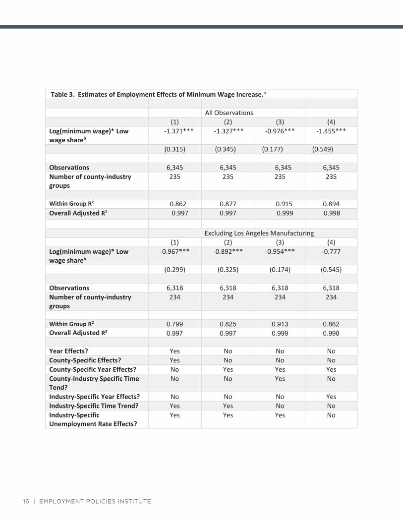
Table 3 presents estimates of our four specifica-tions of the empirical model. The standard errors are corrected for clustering by CIP. The models are estimated with weighting by CIP employment levels. In all four specifications, there is a statis-tically significant (at .01 level) negative effect of minimum wages that is greatest in low wage in-dustries. The range of estimated effects of lmin* low_wage across the four specifications is from -0.98 to -1.46. The standard error of the estimated coefficient is largest in the final model, but this is also the model where the estimated effect of the minimum is greatest.

An important concern with any empirical model is its robustness. We tested the model’s robustness to several changes. First, we examined whether the model’s results were being driven by outliers in the data. To find outliers, we examined wheth-er the coefficients changed sharply by eliminating any given CIP, industry, or county. We discovered that manufacturing in Los Angeles (LA) County had an especially strong impact on the estimat-ed effect of the minimum in some specifications. More careful examination of the data revealed that manufacturing in LA County had a more rap-id downward trend than any other county in the state, and that it was also the county with the highest share of low-wage workers in manufac-turing, and is the county with the highest level of manufacturing employment. The combination of these facts causes the estimated effect of the minimum wage to be less negative when LA coun-ty manufacturing is removed from the data.

Since we are uncomfortable with LA manufactur-ing having such a large effect on the estimates, we also present results with LA County manufacturing removed from the data. The coefficient estimates are substantially reduced in 3 of the 4 specifica-tions, remain negative in all 4 specifications, but becomes statistically insignificant (at the .10 level) in the fourth specification which arguably has the highest degree of collinearity. In specification 3, the exclusion of LA manufacturing has little effect on the estimated minimum wage effect. This is to be expected since this specification allows for a CIP specific time trend which allows LA manu-facturing to have a different time trend than the manufacturing industries in other counties.

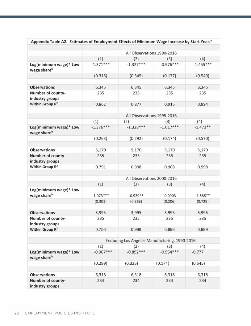
As a second check for robustness, we considered different start dates for the estimation. As noted by Neumark et al. (2014), the estimate of time trends can be sensitive to the end points in the data and can significantly alter the estimated ef-fect of a minimum wage – particularly if the end points include a point where the economy is in recession and the sample period is short. In our case, we have 27 years of data and the economy is not in recession in 2016. Nevertheless, we con-sidered the sensitivity of our results to alterna-tive start dates. The results (available in appendix table A2) indicate that of the 12 different sets of estimates (four regression specifications times 3 different starting points), all 12 of the coefficient estimates are negative and 11 of the 12 are statisti-cally significant at the .05 level. It is worth noting that the statistically insignificant results only oc-cur when the start year is pushed to 2000. This is the shortest sample period considered and also eliminates a very large increase in the minimum wage that occurred in 1998.

If LA County manufacturing is removed from the sample due to its unusually large influence on some of the estimates, all 12 coefficient estimates remain negative though they achieve statistical significance (at the .05 level) in only 7 of the 12 models. The first two specifications (which have less flexibility and less collinearity) are, however, much more stable across all variations considered – whether LA County manufacturing is excluded or the starting year is varied. This is not surprising as the third and fourth specifications have more


collinearity (and flexibility in fitting in the data) and this makes results more sensitive to changes in the data sample.

As yet another test of robustness, we consider the methodology proposed by Meer and West (2016). Their method was designed to address the possi-bility that a change in the minimum wage would affect the rate of growth in employment instead of a shift in the intercept. The Meer-West approach is to use “long-differences” to estimate the effect of minimum wage hikes. The specification is

Where ∆r is a difference operator. For example,

∆rlemp_ijt is the r-period change in log-employ-

ment that occurs between period (t-r) and t. We estimate this long difference corresponding to the four specifications in our earlier regression mod-els, keeping in mind that when differencing across time, for example, CIP specific fixed effects dif-ference out of the model. Similarly, when differ-encing across time, an industry specific time trend becomes an industry specific fixed effect, and a county specific time trend becomes a county spe-cific fixed effect.

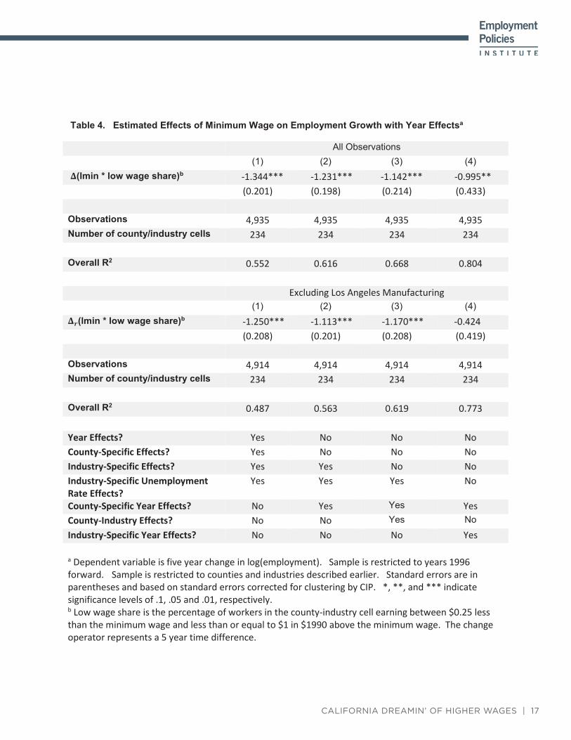
The estimates of the Meer-West model are in ta-ble 4. The estimated models correspond to the time-differenced versions of the four specifica-tions in our earlier analysis of employment levels. In the first four specifications, all observations are included and we present results for the 5-year time difference. In all four specifications, the co-efficient estimates imply a statistically significant (at .01 level) negative effect of minimum wage in-creases on employment growth. We also con-sidered shorter and longer time differences. For most specifications considered, the effects were statistically significant for both shorter and longer time differences6.

Time-differenced models were also estimated with LA County manufacturing excluded. These

are shown in the lower panel of table 4 for a five-year time difference. The first three specifications all yield statistically significant negative minimum wage effects, though the fourth specification is statistically insignificant at the .10 level with a co-efficient that is less than one-half of that found in the other three specifications.

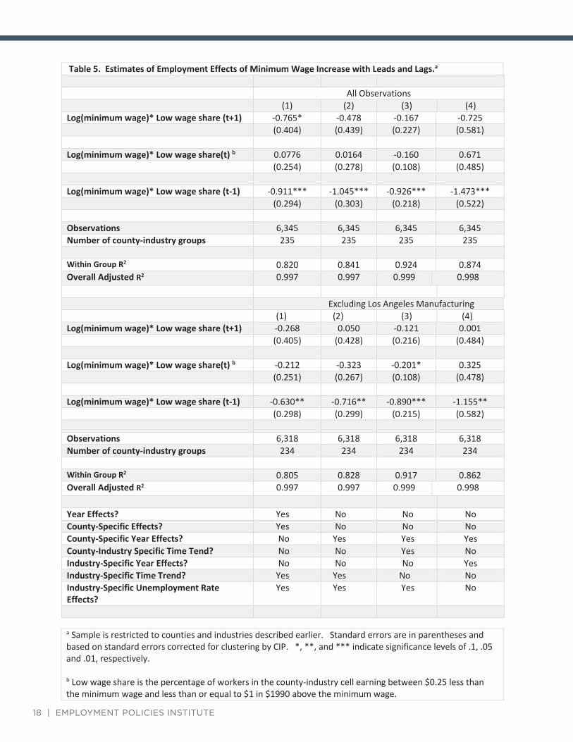
Finally, to assure that the minimum wage effects estimated are not capturing some omitted factor, we examine whether leading and lagging values of the minimum explain employment. If leading val-ues explain employment, one might be concerned that the model is capturing a spurious relationship between the minimum and employment levels. Alternatively, it might be that employers begin re-ducing low wage employment in anticipation of the minimum wage rising.

Table 5 provides estimates of the same models used in table 3, but adds a one year lead and lag of lmin* low_wage to the model. In the model in-cluding all CIPs, the lagged value of the minimum wage has a statistically significant negative effect for all four specifications, the contemporaneous minimum wage is never statistically significant, and the leading value is never statistically signifi-cant at the .05 level7. When the LA County manu-facturing CIP is excluded, the lagged minimum is significant at .05 level in all four models. The lead-ing and contemporaneous effects of the minimum are small and never significant at the .05 level.

In review, we have considered numerous regres-sion models to estimate the effect of minimum wage increases on employment. We found some evidence that the negative effects of the minimum wage are particularly sensitive to the inclusion of the LA County manufacturing CIP. Nevertheless, even after excluding this CIP, most specifications still yield statistically significant negative effects. The most sensitive specifications tend to be those with the most collinearity which leads to less iden-tifying variation in the minimum wage variable. The results are fairly similar in magnitude whether we use employment levels or time-difference the

6 The one exception was the fourth specification where the results were statistically significant only for time differences of 5 years or more.

7The leading value is statistically significant at the .10 level in one of the four specifications.


data. We also find little evidence that leading val-ues of the minimum wage explain changes in em-ployment.

While we consider the results quite robust to al-ternative specifications, we think it is important to note that, given the high degree of flexibility (and thus collinearity) in the models, the estimates can be fairly sensitive to changes in controls and/or time periods. Nevertheless, we believe that the bulk of the evidence points toward substantial negative effects of California minimum wage in-creases on employment – particularly in low wage industries. We turn to the size of these effects in the next section.

To put our range of estimated minimum wage em-ployment effects in perspective, a coefficient of -1 on lmin* low_wage implies that, in an industry where 50% of the workers are paid within $1 of the minimum wage (in 1990 dollars), a 10% in-crease in the minimum causes a 5% decrease in employment. For the average CIP in our sample, the proportion of workers with low wages is 21 percent. As a consequence, our estimated coeffi-cient of -0.89 from our preferred specification (2) with LA County manufacturing excluded implies that a 10% increase in the minimum wage reduces employment in the average industry by 1.9%. This translates into a minimum wage elasticity of -0.19 for all workers. Other studies find a wide range of estimated minimum wage elasticities. For exam-ple, the CBO (2014) reports a range of 0 to -0.20 for teenagers, and 0 to -0.07 for adults. Meer and West (2016) report a minimum wage elastic-ity of -.08 for all workers. More recently, Jardim et al. (2017) summarize a series of studies for the restaurant industry with elasticities ranging from 0.02 to -0.24, though they argue that most previ-ous studies underestimate the elasticities and that the restaurant industry may have a lower elastici-ty than others. Their analysis of the 2016 Seattle Washington minimum wage increase estimates a minimum wage elasticity of -0.23 to -0.28 for all workers8. Overall, our estimated elasticity of

-0.19 for all workers fits within the bounds of ear-lier studies. It is important to note, however, that these elasticities are not entirely comparable be-cause the studies differ in terms of the industries examined, the size of the minimum wage hike, and the fraction of workers impacted by the minimum wage increase.

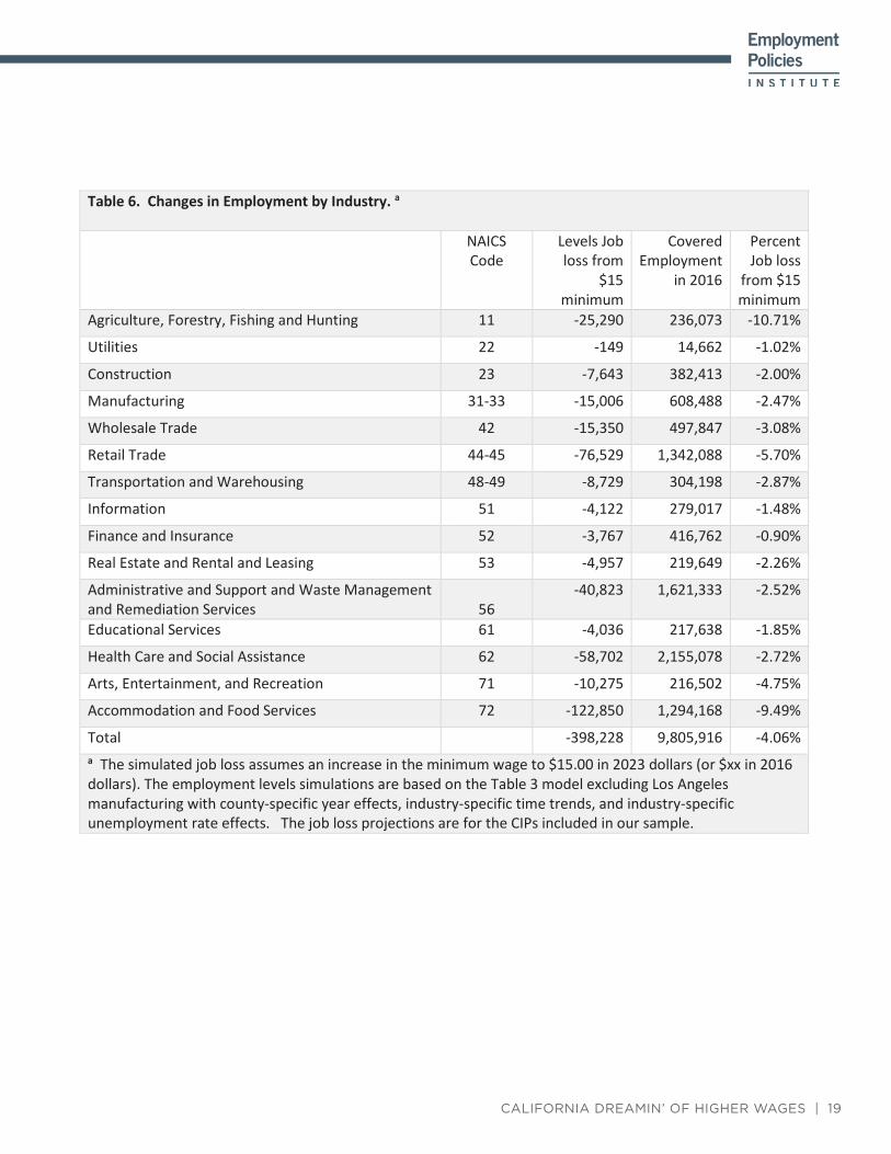
SIMULATIONS OF EMPLOYMENT LOSS FROM A $15 MINIMUM WAGECalifornia’s minimum wage is scheduled to rise from $10.50 in 2017, to $11.00 in 2018, and then increase $1 per year until it reaches $15 in 2022. In this section, we use our earlier econometric es-timates to simulate how many jobs would be lost as a result of this increase. To perform the simula-tion, we estimate the effect of switching to $15 in the 2016 labor market. Since wages will grow over time, we convert the 2022 minimum of $15 into 2016 dollars by assuming that prices will grow at 2.2% per year, which is consistent with the CBO forecast for 2016 to 20229. We then use the sec-ond specification from table 3 that excluded the LA County manufacturing sector to simulate em-ployment loss. This is accomplished by estimating the change in the log of employment that would occur if the minimum wage is increased from the 2016 value of $10.00 (except in San Francisco county where it was $12.25 until July 2016). We then convert the estimated change in log-employ-ment into the change in the level of employment. The results of this simulation are presented by in-dustry in table 6. In total, we estimate that raising the minimum wage to $12.88 (the equivalent of $15 in 2022) will result in a loss of 398,228 jobs in the CIPs included in our sample. This represents 4.1% of the employment in the included CIPs. As a percentage of employment, the estimated job loss is greatest in the two industries with the larg-est share of low-wage workers – agriculture, for-estry and fishing; and accommodation and food

8 While the range of elasticities is -0.23 to -0.28 for all workers, this translates into an elasticity -2.7 to -3.5 for workers who are directly affected by the minimum wage.

9Congressional Budget Office, www.cbo.gov.


services. In these industries, we project 10.7 and 9.5 percent of jobs will be eliminated as a result of a $15 minimum. The size of the predicted job loss is greatest in accommodation and food services (123,000) and retail trade (77,000). These two in-dustries account for half of the predicted job loss in our sample of CIPs.

These simulations are based on what we consider to be the most robust and parsimonious regres-sion model. As we noted, however, the empirical estimates are somewhat sensitive to the types of controls included and the starting point for the sample period. In all, we estimated 24 differ-ent specifications of the employment regression (4 different sets of controls x 3 different starting years x 2 samples that either include or exclude LA county manufacturing). Averaging across these 24 different specifications results in a 11.88 percent greater job loss of 445,000.

SUMMARY AND CONCLUSIONSThis study uses California employment data from 1990 through 2016 to test whether the state’s min-imum wage increases over the past 25 years have led to the loss of low-wage jobs. Our empirical approach identifies the effects of minimum wage increases by comparing the evolution of employ-ment across county-industry pairs (CIPs). We find fairly robust evidence that, when the minimum wage increases, employment growth is slowed in low-wage relative to high-wage CIPs. While our models are parsimonious in terms of our ability to control for observed economic conditions, our models allow for a variety of different types of fixed effects and/or time trends that would control for any common shocks that impact all industries across counties, or all industries within a county. We also examined the data for outliers that might have unusually large effects on our estimates.

Across a wide range of specifications, we find sta-tistically significant negative effects of the Cali-fornia minimum wage increases on employment growth – particularly in low-wage industries. If we

expand the list of controls to the point of having a highly saturated model, the estimates become statistically insignificant. We do not view these in-significant results as evidence against a minimum wage effect. Rather, we believe that if an empiri-cal model includes large numbers of fixed effects there is too much collinearity in the model and too little identifying variation left in minimum wage movements.

Our preferred estimates, which exclude Los An-geles County manufacturing as an outlier, suggest that a 10% increase in the minimum wage would lead to an 4.5% reduction in employment in an in-dustry if one-half of its workers earn low-wages. We use these estimates to simulate the number of jobs that would be lost for the CIPs included in our sample if the minimum wage is increased to $15 in 2022. Our results suggest that approximately 400,000 jobs would be lost in the CIPs included in our sample. This represents about a 4.1% reduction in employment. Approximately one-half of the job loss occurs in accommodations and food services, and retail trade.

While our model provides fairly convincing evi-dence that minimum wage increases to cause job loss, it’s important to note that it is based on his-torical data and that the models assume that the only factor that determines the response of an in-dustry to a minimum wage hike is its share of low wage workers. In reality, the response elasticities of firms to minimum wage hikes will depend on factors such as their ability to replace labor with capital, and labor’s share of the firm’s total cost. The easier it is to substitute capital for labor and the more labor intensive the firm is, the greater the expected response to a change in the mini-mum wage. Moreover, a firm’s ability to pass on the cost of a minimum wage hike may vary over time as new technologies are developed. As a result, our estimates should be considered with some caution given the simplifying assumptions of our model. Nevertheless, we feel that our estimates of job loss are consistent with the employment loss associated with previous minimum wage increas-es in California.


REFERENCES

Autor, David H.; Dorn, David. “The Growth of Low-Skill Service Jobs and the Polarization of the US Labor Market.” American Economic Review 103 (December 2013): 1553-1597.

Autor, David H.; Dorn, David; and Hanson, Gordon H. “The China Syndrome: Local Labor Market Effects of Import Competition in the United States.” American Economic Review 103 (December 2013): 2121-2168.

_______________. “Untangling Trade and Technology: Evidence From Local Labor Markets.” The Eco-nomic Journal 125 (May 2015): 621–646.

Baily, Martin Neil and Bosworth, Barry P. “U.S. Manufacturing: Understanding Its Past and Its Potential Future.” The Journal of Economic Perspectives 28 (Winter 2014): 3-25.

Congressional Budget Office. “The Effects of a Minimum-Wage Increase on Employment and Family In-come.” February 2014.

Jardim, Ekaterina; Long, Mark C.; Plotnick, Robert; Inwegen, Emma van; Vigdor, Jacob; and Wething; Hilary. “Minimum Wage Increases, Wages, and Low-Wage Employment: Evidence From Seattle.” NBER Working Paper Number 23552, June 2017.

Pierce, Justin R. and Schott, Peter K. “The Surprisingly Swift Decline of US Manufacturing Employment.” American Economic Review 106 (July 2016): 1632-62.

Meer, Jonathan and West, Jeremy. “Effects of the Minimum Wage on Employment Dynamics.” Journal of Human Resources 51 (Spring 2016): 500-522.

Neumark, David. “The Effects of Minimum Wages on Employment.” FRBSF Economic Letter, December 21, 2015.

Neumark, David; Salas, J. M. Ian; and Wascher, William. “Revisiting the Minimum Wage-Employment De-bate: Throwing Out the Baby with the Bathwater?” Industrial and Labor Relations Review 67 (May 2014): 608-648.

Neumark, David, and Wascher, William. Minimum Wages. Cambridge, MA: MIT Press, 2008.


15


16


17

Table 1. Counties Included in Analysis. County County

FIPS Code 2016

Employment Covered by

Industries with complete data for 1990-2016

Total County Employment in

2016

Share of 2016

employment covered in

data.

Butte 7 51,800 64,366 80.5% El Dorado 17 21,196 42,494 49.9% Fresno 19 233,795 303,441 77.0% Kern 29 229,155 243,339 94.2% Los Angeles 37 3,665,722 3,756,230 97.6% Merced 47 32,320 57,991 55.7% Monterey 53 126,861 154,346 82.2% Orange 59 1,352,394 1,397,182 96.8% Placer 61 89,314 136,349 65.5% Riverside 65 461,702 559,878 82.5% Sacramento 67 446,642 461,371 96.8% San Bernardino 71 528,594 577,448 91.5% San Diego 73 1,085,212 1,167,110 93.0% San Francisco 75 518,639 600,645 86.3% San Joaquin 77 160,204 194,765 82.3% San Luis Obispo 79 82,302 93,057 88.4% San Mateo 81 254,753 356,677 71.4% Santa Barbara 83 151,470 161,737 93.7% Solano 95 44,465 110,002 40.4% Sonoma 97 151,004 173,130 87.2% Stanislaus 99 113,895 152,909 74.5% Tulare 107 65,967 127,898 51.6% Ventura 111 255,966 275,707 92.8% Yolo 113 42,136 67,438 62.5% All Included Counties 10,165,508 11,235,510 90.5% California 14,126,759 72.0%


18

Table 2. Industries Covered in Analysis.1 Industry NAICS

Code Number

of Counties

2016 Covered

Employment Total

Average share of county

employment in 2016

Covered Employment

Share of State Employment

Total

2016 State

Employment Total

Agriculture, Forestry, Fishing and Hunting 11 10 236,073 11.2% 57.76% 408,690

Utilities 22 4 14,662 0.4% 25.03% 58,578 Construction 23 9 382,413 5.5% 50.85% 752,044 Manufacturing 31-33 22 968,080 8.4% 74.98% 1,291,140 Wholesale Trade 42 16 497,847 4.1% 69.82% 713,060 Retail Trade 44-45 24 1,342,088 13.1% 81.46% 1,647,523 Transportation and Warehousing 48-49 9 304,198 3.7% 61.25% 496,663 Information 51 10 279,017 1.9% 54.12% 515,558 Finance and Insurance 52 19 416,762 3.4% 77.48% 537,898 Real Estate and Rental and Leasing 53 20 219,649 1.8% 80.47% 272,963 Administrative and Support and Waste Management and Remediation Services

56

17

1,621,333 13.5%

71.48%

2,268,315

Educational Services 61 14 217,638 1.8% 70.83% 307,270 Health Care and Social Assistance 62 24 2,155,078 19.3% 80.97% 2,661,619 Arts, Entertainment, and Recreation 71 14 216,502 1.9% 73.90% 292,972 Accommodation and Food Services 72 23 1,294,168 11.8% 82.38% 1,571,030 Total 10,165,508 73.69% 13,795,321 1. Employment counts are for the counties included in the analysis. See table 1 for list of counties. 2016 data is based on January through June of 2016 data. 2 Percent of workers with low wages [i.e. earning between $0.25 in nominal terms less than the minimum and less than or equal to $1 (in 1990 dollars) above the minimum] is calculated for each NAICS industry using 1996-2016 data from Current Population Survey for California, excluding all counties other than San Francisco County with a local minimum wage ordinance.


19

Table 3. Estimates of Employment Effects of Minimum Wage Increase.a All Observations (1) (2) (3) (4) Log(minimum wage)* Low wage shareb

-1.371*** -1.327*** -0.976*** -1.455***

(0.315) (0.345) (0.177) (0.549) Observations 6,345 6,345 6,345 6,345 Number of county-industry groups

235 235 235 235

Within Group R2 0.862 0.877 0.915 0.894 Overall Adjusted R2 0.997 0.997 0.999 0.998 Excluding Los Angeles Manufacturing (1) (2) (3) (4) Log(minimum wage)* Low wage shareb

-0.967*** -0.892*** -0.954*** -0.777


234 234 234 234

Within Group R2 0.799 0.825 0.913 0.862Overall Adjusted R2 0.997 0.997 0.999 0.998 Year Effects? Yes No No No County-Specific Effects? Yes No No No County-Specific Year Effects? No Yes Yes Yes County-Industry Specific Time Tend?

No No Yes No

Industry-Specific Year Effects? No No No Yes Industry-Specific Time Trend? Yes Yes No No Industry-Specific Unemployment Rate Effects?

Yes Yes Yes No


20

Table 4. Estimated Effects of Minimum Wage on Employment Growth with Year Effectsa

All Observations(1) (2) (3) (4)

𝚫𝚫𝚫𝚫(lmin * low wage share)b -1.344*** -1.231*** -1.142*** -0.995** (0.201) (0.198) (0.214) (0.433)

Observations 4,935 4,935 4,935 4,935 Number of county/industry cells 234 234 234 234

Overall R2 0.552 0.616 0.668 0.804

Excluding Los Angeles Manufacturing(1) (2) (3) (4)

𝚫𝚫𝚫𝚫𝒓𝒓𝒓𝒓(lmin * low wage share)b -1.250*** -1.113*** -1.170*** -0.424 (0.208) (0.201) (0.208) (0.419)

Observations 4,914 4,914 4,914 4,914 Number of county/industry cells 234 234 234 234

Overall R2 0.487 0.563 0.619 0.773 Year Effects? Yes No No NoCounty-Specific Effects? Yes No No NoIndustry-Specific Effects? Yes Yes No NoIndustry-Specific Unemployment Rate Effects?

Yes Yes Yes No

County-Specific Year Effects? No Yes Yes Yes County-Industry Effects? No No Yes No Industry-Specific Year Effects? No No No Yes

a Dependent variable is five year change in log(employment). Sample is restricted to years 1996 forward. Sample is restricted to counties and industries described earlier. Standard errors are in parentheses and based on standard errors corrected for clustering by CIP. *, **, and *** indicate significance levels of .1, .05 and .01, respectively. b Low wage share is the percentage of workers in the county-industry cell earning between $0.25 less than the minimum wage and less than or equal to $1 in $1990 above the minimum wage. The change operator represents a 5 year time difference.


21

Table 5. Estimates of Employment Effects of Minimum Wage Increase with Leads and Lags.a All Observations (1) (2) (3) (4) Log(minimum wage)* Low wage share (t+1) -0.765* -0.478 -0.167 -0.725 (0.404) (0.439) (0.227) (0.581) Log(minimum wage)* Low wage share(t) b 0.0776 0.0164 -0.160 0.671 (0.254) (0.278) (0.108) (0.485) Log(minimum wage)* Low wage share (t-1) -0.911*** -1.045*** -0.926*** -1.473*** (0.294) (0.303) (0.218) (0.522) Observations 6,345 6,345 6,345 6,345 Number of county-industry groups 235 235 235 235 Within Group R2 0.820 0.841 0.924 0.874 Overall Adjusted R2 0.997 0.997 0.999 0.998 Excluding Los Angeles Manufacturing (1) (2) (3) (4) Log(minimum wage)* Low wage share (t+1) -0.268 0.050 -0.121 0.001 (0.405) (0.428) (0.216) (0.484) Log(minimum wage)* Low wage share(t) b -0.212 -0.323 -0.201* 0.325 (0.251) (0.267) (0.108) (0.478) Log(minimum wage)* Low wage share (t-1) -0.630** -0.716** -0.890*** -1.155** (0.298) (0.299) (0.215) (0.582) Observations 6,318 6,318 6,318 6,318 Number of county-industry groups 234 234 234 234 Within Group R2 0.805 0.828 0.917 0.862 Overall Adjusted R2 0.997 0.997 0.999 0.998 Year Effects? Yes No No No County-Specific Effects? Yes No No No County-Specific Year Effects? No Yes Yes Yes County-Industry Specific Time Tend? No No Yes No Industry-Specific Year Effects? No No No Yes Industry-Specific Time Trend? Yes Yes No No Industry-Specific Unemployment Rate Effects?

Yes Yes Yes No

22

a Sample is restricted to counties and industries described earlier. Standard errors are in parentheses and based on standard errors corrected for clustering by CIP. *, **, and *** indicate significance levels of .1, .05 and .01, respectively. b Low wage share is the percentage of workers in the county-industry cell earning between $0.25 less than the minimum wage and less than or equal to $1 in $1990 above the minimum wage.


23

Table 6. Changes in Employment by Industry. a NAICS

Code Levels Job loss from

$15 minimum

Covered Employment

in 2016

Percent Job loss

from $15 minimum

Agriculture, Forestry, Fishing and Hunting 11 -25,290 236,073 -10.71%

Utilities 22 -149 14,662 -1.02%

Construction 23 -7,643 382,413 -2.00%

Manufacturing 31-33 -15,006 608,488 -2.47%

Wholesale Trade 42 -15,350 497,847 -3.08%

Retail Trade 44-45 -76,529 1,342,088 -5.70%

Transportation and Warehousing 48-49 -8,729 304,198 -2.87%

Information 51 -4,122 279,017 -1.48%

Finance and Insurance 52 -3,767 416,762 -0.90%

Real Estate and Rental and Leasing 53 -4,957 219,649 -2.26%

Administrative and Support and Waste Management and Remediation Services

56

-40,823 1,621,333 -2.52%

Educational Services 61 -4,036 217,638 -1.85%

Health Care and Social Assistance 62 -58,702 2,155,078 -2.72%

Arts, Entertainment, and Recreation 71 -10,275 216,502 -4.75%

Accommodation and Food Services 72 -122,850 1,294,168 -9.49%

Total -398,228 9,805,916 -4.06% a The simulated job loss assumes an increase in the minimum wage to $15.00 in 2023 dollars (or $xx in 2016 dollars). The employment levels simulations are based on the Table 3 model excluding Los Angeles manufacturing with county-specific year effects, industry-specific time trends, and industry-specific unemployment rate effects. The job loss projections are for the CIPs included in our sample.


24

Appendix Table A1. Federal and California State Minimum Wage

Year Federal Minimum Wage California Minimum Wagea

1939 $0.25 $0.33 1940 $0.40 $0.33 1941 $0.40 $0.33 1942 $0.40 $0.33 1943 $0.40 $0.33 1944 $0.40 $0.45 1945 $0.40 $0.45 1946 $0.40 $0.45 1947 $0.40 $0.45 1948 $0.40 $0.65 1949 $0.40 $0.65 1950 $0.75 $0.65 1951 $0.75 $0.65 1952 $0.75 $0.65 1953 $0.75 $0.75 1954 $0.75 $0.75 1955 $0.75 $0.75 1956 $0.75 $0.75 1957 $1.00 $0.75 1958 $1.00 $1.00 1959 $1.00 $1.00 1960 $1.00 $1.00 1961 $1.00 $1.00 1962 $1.15 $1.00 1963 $1.15 $1.00 1964 $1.15 $1.25 1965 $1.15 $1.30 1966 $1.15 $1.30 1967 $1.15 $1.30 1968 $1.40 $1.30 1969 $1.60 $1.65 1970 $1.60 $1.65 1971 $1.60 $1.65 1972 $1.60 $1.65 1973 $1.60 $1.65 1974 $1.60 $1.65 1975 $2.10 $2.00 1976 $2.30 $2.00 1977 $2.30 $2.50 1978 $2.65 $2.50 1979 $2.90 $2.90


25

1980 $3.10 $3.10 1981 $3.35 $3.35 1982 $3.35 $3.35 1983 $3.35 $3.35 1984 $3.35 $3.35 1985 $3.35 $3.35 1986 $3.35 $3.35 1987 $3.35 $3.35 1988 $3.35 $3.35 1989 $3.35 $4.25 1990 $3.35 $4.25 1991 $3.80 $4.25 1992 $4.25 $4.25 1993 $4.25 $4.25 1994 $4.25 $4.25 1995 $4.25 $4.25 1996 $4.25 $4.25 1997 $4.75 $4.75 1998 $5.15 $5.15 1999 $5.15 $5.75 2000 $5.15 $5.75 2001 $5.15 $6.25 2002 $5.15 $6.75 2003 $5.15 $6.75 2004 $5.15 $6.75 2005 $5.15 $6.75 2006 $5.15 $6.75 2007 $5.15 $7.50 2008 $5.85 $8.00 2009 $6.55 $8.00 2010 $7.25 $8.00 2011 $7.25 $8.00 2012 $7.25 $8.00 2013 $7.25 $8.00 2014 $7.25 $9.00 2015 $7.25 $9.00 2016 $7.25 $10.00 2017 $7.25 $10.50 2018 $7.25 $11.00 2019 $7.25 $12.00 2020 $7.25 $13.00 2021 $7.25 $14.00 2022 $7.25 $15.00

a Between January 2017 and January 2023, California state law has a lower minimum wage for employers with 25 employers or less.


26

Appendix Table A2. Estimates of Employment Effects of Minimum Wage Increase by Start Year.a All Observations 1990-2016 (1) (2) (3) (4) Log(minimum wage)* Low wage shareb

-1.371*** -1.327*** -0.976*** -1.455***


235 235 235 235

Within Group R2 0.862 0.877 0.915 0.894 All Observations 1995-2016 (1) (2) (3) (4) Log(minimum wage)* Low wage shareb

-1.376*** -1.328*** -1.017*** -1.473**


235 235 235 235

Within Group R2 0.791 0.998 0.908 0.998 All Observations 2000-2016 (1) (2) (3) (4) Log(minimum wage)* Low wage shareb -1.073*** -0.929** -0.0903 -1.588** (0.301) (0.363) (0.206) (0.729) Observations 3,995 3,995 3,995 3,995 Number of county-industry groups

235 235 235 235

Within Group R2 0.756 0.998 0.898 0.999 Excluding Los Angeles Manufacturing, 1990-2016 (1) (2) (3) (4) Log(minimum wage)* Low wage shareb

-0.967*** -0.892*** -0.954*** -0.777


234 234 234 234


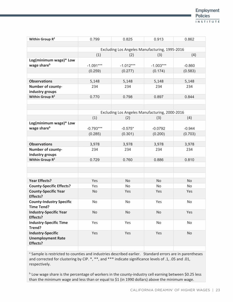
27

Within Group R2 0.799 0.825 0.913 0.862 Excluding Los Angeles Manufacturing, 1995-2016 (1) (2) (3) (4) Log(minimum wage)* Low wage shareb -1.091*** -1.012*** -1.003*** -0.860 (0.259) (0.277) (0.174) (0.583) Observations 5,148 5,148 5,148 5,148 Number of county-industry groups

234 234 234 234

Within Group R2 0.770 0.798 0.897 0.844 Excluding Los Angeles Manufacturing, 2000-2016 (1) (2) (3) (4) Log(minimum wage)* Low wage shareb -0.793*** -0.575* -0.0792 -0.944 (0.285) (0.301) (0.200) (0.703) Observations 3,978 3,978 3,978 3,978 Number of county-industry groups

234 234 234 234

Within Group R2 0.729 0.760 0.886 0.810 Year Effects? Yes No No No County-Specific Effects? Yes No No No County-Specific Year Effects?

No Yes Yes Yes

County-Industry Specific Time Tend?

No No Yes No

Industry-Specific Year Effects?

No No No Yes

Industry-Specific Time Trend?

Yes Yes No No

Industry-Specific Unemployment Rate Effects?

Yes Yes Yes No

a Sample is restricted to counties and industries described earlier. Standard errors are in parentheses and corrected for clustering by CIP. *, **, and *** indicate significance levels of .1, .05 and .01, respectively. b Low wage share is the percentage of workers in the county-industry cell earning between $0.25 less than the minimum wage and less than or equal to $1 (in 1990 dollars) above the minimum wage.


NOTES


EPIONLINE.ORG

Documents

California Dreamin’ of Higher Wages · California Dreamin’ of Higher Wages William E. Even Raymond E. Glos Professor of Economics | Miami University David A. Macpherson E.M. Stevens