VYTAUTAS MAGNUS UNIVERSITY

FACULTY OF INFORMATICS

DEPARTMENT OF APPLIED INFORMATICS

Huseyn Gadirov

Capsule Architecture as a Discriminator in Generative Adversarial Networks

Master Thesis

APPLIED INFORMATICS Study Programme, State code: 621I13003

Field of study: Informatics

Supervisor Minija Tamošiūnaitė

Moksl. laipsnis, vardas, pavardė signature, date

Defended Daiva Vitkute-Adzgauskiene

Fakulteto dekanas signature, date

Kaunas, 2018

CONTENT

CONTENT ……………………………………………………………………………….….. 1

ABBREVIATION AND TERM DICTIONARY ………………………………....……....…. 3

ABSTRACT ………………………………………………………………...…....….……..... 4

1 INTRODUCTION …………………………......………….…………………………. 5

2 RELATED WORK …...………………………………....…………………………… 7

3 CAPSULE LAYERS ………….……..……..…………………………….......……… 9

4 ROUTING BY AGREEMENT ……………………..…………………………....…. 12

5 INCORPORATING A CAPSULE NETWORK IN GENERATIVE ADVERSARIAL NETWORKS …………………….……………………………..……….………………...… 13

5.1 DCGAN ………………..……………………...………………………………..…… 15

6 DATASETS ………………..…………..……...…………………………………….. 16

7 METHODOLOGY …………….…………...……….………………………............. 16

7.1 DISCRIMINATOR STRUCTURE ……………….…………………....………..….. 17

7.2 GENERATOR STRUCTURE ……...………………….…………………...……..… 19

8 RESULTS ……………..……………………...……………………………...…....… 20

8.1 QUALITATIVE EVALUATION ………......……….…………………………...….. 21

8.2 QUANTITATIVE EVALUATION ……………….……………………………...…. 22

8.2.1 INCEPTION SCORE ……...…………….…………….…………………….…...…. 24

9 DISCUSSION ……………..……………………...………………………......…..… 26

10 FURTHER RESEARCH ………......……….…………………………………....….. 26

11 CONCLUSION …………………………..……….…………………....………...…. 27

REFERENCES ………...………………………………………………………….….28

1

APPENDICES ………………………………………………………………..…….. 31

2

ABBREVIATION AND TERM DICTIONARY

Neural Network NN

Variational Autoencoder VAE

Deep Learning DL

Convolutional Neural Network CCN

Generative Adversarial Network GAN

Deep Convolutional Generative Adversarial Network DCGAN

Boundary Equilibrium Generative Adversarial Networks BEGAN

Mixture Generative Adversarial Nets MGAN

Jensen-Shannon Divergence JSD

Rectified Linear Unit ReLU

Graphics Processing Unit GPU

Amazon Mechanical Turk AMT

Inception Score IS

Kullback–Leibler divergence KL

3

ABSTRACT

Author Huseyn Gadirov

Title Capsule Architecture as a Discriminator in Generative Adversarial Networks

Supervisor prof. Minija Tamošiūnaitė

Number of pages 30

Number of tables 1

Number of pictures 9

Number of appendices 1

Modern convolutional networks are good at detecting objects in the scene but have a hard time

identifying the position of one object relative to another. This exposes certain limitations to the model

such as losing the spatial relationships between features. A recent solution to that problem is relying on

“Capsules” - a logistic unit that represents the presence of the object as well as the relationship between

that entity and the pose. Meanwhile, this paper focuses on incorporating the Capsule architecture into

the Discriminator of the Generative Adversarial Networks instead of the conventional convolutions,

which is able to lead to a better classification loss and faster convergence. We describe the architecture,

main differences from the original paper on Capsules and evaluate the results both qualitatively and

quantitatively. Finally, we suggest possible improvements and thoughts on ideas worth investigating.

4

1. INTRODUCTION

Since 2012, when Convolutional Neural Networks (CNNs) showed significantly better performance

than any previous method on image classification task for ImageNet, they have been the standard

approach for Computer Vision. As per the goal of this paper, Image Generation is one of the task

subcategories of the modern Computer Vision that is done with Neural Networks and CNNs, in

particular - Generative models such as Variational Autoencoders (VAEs), Restricted Boltzmann

Machines or Generative Adversarial Networks (GANs). But what exactly is “Image Generation”? Let

us make it more concrete. Suppose we have a large image dataset. These images are the samples from

the true data distribution or in other words they represent how the world looks like. A generative model

in our case, outputs images that are drawn from the real distribution and we refer to those as “samples

from the model”. Under the hood, it discovers the most representational features from our data, such as:

color correlation of the pixels nearby, horizontal and vertical lines and how exactly is our world made

from them. Eventually, the model can also discover complex features, such as: objects, textures, certain

types of backgrounds or how they are arranged in the space over time if it is a video [1]. Next we dive

deeper into how CNNs work, point out the drawbacks and suggest an architectural change that can

impact the Image Generation.

In short, CNNs can detect the presence of features in the image and predict whether an object exists by

feeding the knowledge of these features forward. However, the problem with CNNs is that they only

detect the existence of features . A contorted face image which contains a misplaced eye, nose, and

ear, would still be considered a face since it comprises of all the necessary features. CNN is good at

detecting features, however, less viable at exploring the spatial connections among features such as

point of view, size or orientation [2]. That downside of CNNs implies - we do not have an internal

representation of the data; the main learning we have is originating from the data itself. For instance, if

we want to be able to identify cars in numerous perspectives we need to have these car images from a

different viewpoint in the training set, since we did not encode the earlier knowledge of the geometrical

relationship into the network [2].

An important thing to comprehend about CNNs is that throughout the training, higher-level features

tend to combine lower-level features as a weighted sum: activations of a preceding layer are multiplied

by the following layer neuron’s weights and added, before being passed to activation nonlinearity. This

5

strategy contains no pose connection between simpler features that make up a higher level feature.

CNN way to deal with this issue is to utilize Max Pooling or convolutional layers with bigger strides

that reduce spacial size of the information flowing through the network and therefore increase the

“field of view” of higher layers, thus allowing them to detect higher order features in a bigger region of

the input image [2].

Other than reducing the size of the feature vector Max Pooling has some other ideas behind it. By only

considering the max, we essentially are only interested if a feature is present in a certain window but

we generally do not really care about the exact location [4]. If we have a convolution filter, which

detects edges, an edge will give a high response to this filter and the Max Pooling only keeps the

information if an edge is present and throws away “unnecessary” information which also include the

location and the spatial relationship between certain features [4].

Approaches with Max Pooling have a tremendous effect on convolutional networks and work

shockingly well, accomplishing superhuman performance in numerous areas, nevertheless it is losing

valuable information along the way. Hinton himself stated that the fact that Max Pooling is working so

well is a major oversight: “The pooling operation used in convolutional neural networks is a big

mistake and the fact that it works so well is a disaster.” Moreover Max Pooling is, according to Hinton,

a unrefined way to redirect information to the maximum, there are other ways to redirect which are

more complex than a straightforward Max Pooling.

If we think of Computer Graphics, Capsules can model internal hierarchical representation of data, by

combining several matrices to model the relationship of certain parts of an object [3]. From a biological

perspective, whenever we recognize an object with our brain we play out some sort of inverse graphics

solutions; from visual information received by eyes, they deconstruct a leveled representation of the

world around us and try to match it with already learned patterns and relationships put away in the

brain. This is how recognition happens. And the key idea is that representation of objects in the brain

does not depend on view angle. It simply needs to make the inward representation happen in a NN.

Motivated by GANs success for image generation and modelling the distribution of the input data with

its attributes as well as ability to be applied to different tasks ranging from style transfer to image

translation, we incorporate the Capsule architecture into the Discriminator of the GAN, therefore

changing the overall intuition towards a more robust way of capturing the equavariance of the detected

6

features. We train and evaluate our model using MNIST and CIFAR-10 datasets in the following

sections.

2. RELATED WORK

There have been a lot of research on GANs and its different variations, especially with convolutional

GANs (for ex. DCGAN [5] that we are using), less research on Capsule Networks and no previous

experiments on blending those two. Since the original GAN did not perform well on slightly

sophisticated datasets such as CIFAR-10, time by time many different proposals were made in order to

improve its performance and make it robust for applying to other datasets. Some of such attempts are

DCGAN, BEGAN [6], Wasserstein GAN [7] that were explicitly targeting the discriminators,

generators and losses.

Here we describe papers and architectures that highly relate to ours in terms of the intuition behind

proposing an architectural change to any parts of the GAN.

Quan et al. [8] proposed a Mixture Generative Adversarial Networks (MGAN) architecture with a new

approach of training the GANs with a mixture of generators in order to overcome the mode collapsing

problem. The main intuition is to employ multiple generators, instead of using a single one as in the

original GAN paper. Although there is no mentioned modifications to the discriminator - constructing

an ensemble from multiple generators, and randomly selecting one of them as final output, similar to

the mechanism of a probabilistic mixture model, is a method of a complete replacement of the plain old

GAN architecture. They develop theoretical analysis to prove that, at the equilibrium, the

Jensen-Shannon divergence (JSD) between the mixture of generators’ distributions and the base data

distribution is minimal, whilst the JSD among generators’ distributions is maximal, therefore

effectively avoiding the mode collapsing problem - “... by utilizing parameter sharing, our proposed

model adds minimal computational cost to the standard GAN, and thus can also efficiently scale to

large-scale datasets”.

Li et. al [9], however, do not modify much the existing discriminator and generator architectures but

rather introduce an additional 3rd player inside of a GAN called “classifier”. The generator and

7

classifier deal with the conditional distributions between image samples and labels, but the

discriminator focuses only on identifying fake image pairs.

While the previously mentioned approaches introduce some structural difference to parts that GANs

consist of, the most related and recent paper so far is “CapsuleGAN: Generative Adversarial Capsule

Network” by Jaiswal et al [10]. The paper focuses exactly on the same problem of incorporating the

Capsule Network architecture into the GAN, but nevertheless has some distinct parts from ours. In fact

the paper Jaiswal et al. mostly sticks to the original Capsule Network implementation and even uses the

margin loss as an loss function:

(Eq. 1) max V (D, ) E [− (D(x), T ] E [− D(G(x)), T ]minG D G = x∼P data(x) Lm = 1 + z∼P (z)zLm = 0

where is an expected value from the data distribution, is an value from the prior Ex∼P data(x) E z∼P (z)z

distribution, is the margin loss and is a constant. We, however, keep the pixel-wise independent Lm T

mean-square error function from DCGAN instead of the margin loss. The second distinct point is

replacement some of the squashing functions with Leaky ReLU activations and introducing Batch

Normalization. Those can be considered as direct improvements to the model since it was observed that

the networks performs better in this case. And the last but not least, Jaiswal et al. make use of the

Generative Adversarial Metric (GAM) from Im et al. [11] as a pairwise comparison metric. The GAM

approach focuses on directly comparing two generative adversarial models by having them engage in a

“battle” against each other. “The naive intuition is that because every generative adversarial models

consists of a discriminator and a generator in pairs, we can exchange the pairs and have them play the

generative adversarial game against each other.” GAM is represented by following formulas:

(Eq. 2)rtest = ε (D (x )2 test

ε (D (x ))1 test

and

8

(Eq. 3)rsamples = ε (D (G (z)))2 2

ε (D (G (z)))1 1

where outputs the classification error rate and is the predefined test. These ratios eventually (·)ε x test

allow us to compare performances of different models. We on the other hand, carry out our quantitative

evaluation by means of the Inception Score from Zhou et al. [12] that will be discussed in the

upcoming “Results” section. So in conclusion, the three main differences between our and Jaiswal et

al.s’ paper are the following:

● cost function

● different/extra activation function and batch normalization

● evaluation metric

3. CAPSULE LAYERS

Capsule Networks characterize a unique structure within a CNN by dividing neurons into numerous

little gatherings of neurons called “capsules” [13]. Moreover, those capsules capture not only the

likelihood but also the parameters of the specific feature that we will discuss later. Rather than catching

the viewpoint invariance in the activities of “neurons” that use a single scalar output to summarize the

activities of a local pool of replicated feature detectors, instead “capsules” encapsulate the results of

these computations into a small vector of informative outputs. During the training process the

probability of the visual entity being present is locally invariant , that is  it does not change as the

entity changes the position inside the viewport surface of possible appearances within the limited

domain covered by the capsule. However, the instantiation parameters are “equivariant”  -  as the

viewing conditions change and the entity moves over the appearance surface, capsule values change by

a corresponding amount because they are representing the intrinsic coordinates of the entity on the

appearance manifold [14]. Here is the visual representation of network architecture from Sabour’s

paper:

9

Figure 1. Overall architecture of the Capsule Network according to Sabour et al. [13]. This architecture is the main

component of the Discriminator network of our GAN. The input during the runtime is either an image from the dataset or a

Generator output, while the output is a probability score between 0 and 1 indicating whether the input image is real or fake.

As we mentioned before capsules contain probability of a feature detection as the length of the (x)P

output vector, while the geometrical state of the detected feature is encoded as the direction which that

vector points to. In other words, when a detected object changes its position on the image or its state

somehow changes, the length of vector indicating probability stays the same, but its orientation

changes. As an example, in case a capsule detects a face in the image and outputs a 3D vector of length

0.90, at by the time we start moving the face across the image - the vector will rotate in its hyperplane,

representing the changing state of the detected face, but its length will remain fixed, since the capsule is

still sure it has detected a face. This is the thing that G. Hinton alludes to as activities equivariance:

neuronal activities will change when an object “moves over the manifold of possible appearances”

[15].

Equivariance mentioned above is the condition of detected objects that can transform to each other

easily. By learning the feature variance in a capsule, it is possible to extrapolate possible variations

more viably with less training data. Meanwhile, detection probabilities remain constant. This is the

form of invariance that we should aim at, instead of the type offered by CNNs with Max Pooling [15].

While higher capsules receive vectors from lower ones, the length of received vectors indicate

probabilities of low levels detecting their particular objects. These vectors, let us call them , are then ui

multiplied by corresponding weight matrices (transformation matrix) that encode important spatial W

and other important relationships between lower and higher level features. Similar intuitions can be

10

drawn for matrices coming from other neurons and . After multiplication by these weight W 1j W 3j

matrices, what we achieve is the predicted position of the higher level features. In other words, ui︿

represents where one object should be according to the detected positions of lower layer objects:

(Eq. 4) uu︿ j|i = W ij i

where is a transformation matrix, is a vector output of the previous capsule which encodes W ij ui

existence and pose of the object in the image and is a prediction vector [13]. For each parent on the u︿

layer, the corresponding capsule computes a “prediction vector”. It computes it by multiplying its own

output by a weight matrix. In cases where this prediction vector has a large scalar product value with

the output of a possible parent, there is top-down feedback which increases the coupling coefficient for

that parent and decreasing it for other parents [13].

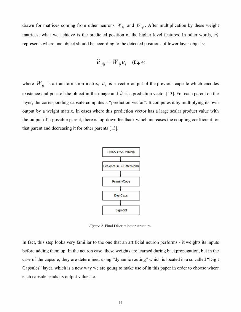
Figure 2. Final Discriminator structure.

In fact, this step looks very familiar to the one that an artificial neuron performs - it weights its inputs

before adding them up. In the neuron case, these weights are learned during backpropagation, but in the

case of the capsule, they are determined using “dynamic routing” which is located in a so called “Digit

Capsules” layer, which is a new way we are going to make use of in this paper in order to choose where

each capsule sends its output values to.

11

4. ROUTING BY AGREEMENT

This section describes routing of outputs from layer to layer in details. This procedure is used l l + 1

to replace Max Pooling from CNNs. As we mentioned in Chapter 3, our network learns transformation

matrices, or simply weights, as the associations between capsules. However, in addition to using these

transformation matrices to route information from layer to layer, each connection is also multiplied by

a coupling coefficient that is also dynamically computed.C ij

In order to make its decision, capsules adjusting the weights (coupling coefficient) that will multiply C

this capsule’s output before sending it to one of the higher layer capsules. We define as a softmax C

over :b

(Eq. 5)C ij =exp bij

Σ exp bk ik

where is the similarity score that takes into account both probability and the feature properties, bij

rather than considering only probability in neurons. Furthermore, will remain low if the activation bij

of capsule is low since length is proportional to : ui i u︿ j|i ui

(Eq. 6) bij ← bij + u︿ j|i · vj

Since are coupling coefficients that are calculated by the iterative dynamic routing process C ij

(discussed next) and are designed to sum to one, conceptually, it measures how likely capsule C Σ ij ii

may activate capsule .jj

12

(Eq. 7) C u sj = Σi ij︿

j|i

where is the output of the higher capsule after routing. However, the routing is not yet finished with sj

that. The squashing function is applied to the output before outputting a value:

(Eq. 8)vj =|| s || j

2

1+ || s || j2 ·

sj

|| s ||j

where is denoted as an output of a squashing function. This type of “routing-by-agreement” turns vj

out to be far more effective than the very primitive form of routing implemented by Max Pooling, that

allows neurons in one layer to ignore all but the most active feature detector in a local pool in the layer

below [13]. Our paper uses a simplified routing algorithm by not vectorizing the DigitCaps values and

replacing the final squashing function with a ReLU nonlinearity:

(Eq. 9)(x) ax (0, x) f = m

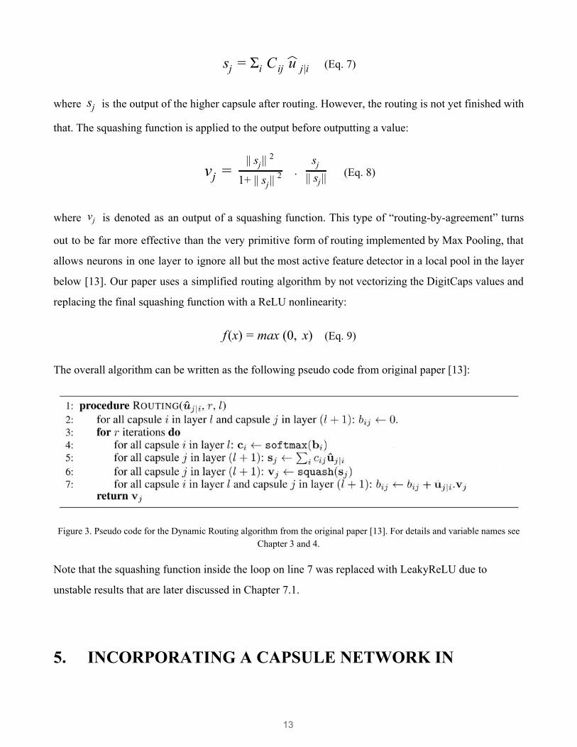
The overall algorithm can be written as the following pseudo code from original paper [13]:

Figure 3. Pseudo code for the Dynamic Routing algorithm from the original paper [13]. For details and variable names see

Chapter 3 and 4.

Note that the squashing function inside the loop on line 7 was replaced with LeakyReLU due to

unstable results that are later discussed in Chapter 7.1.

5. INCORPORATING A CAPSULE NETWORK IN

13

GENERATIVE ADVERSARIAL NETWORKS

The Generative Adversarial Networks (GAN) [17] is framework for establishing a min-max

adversarial game between two neural networks – a generative model - , and a discriminative model - G

. GANs learn to synthesise new samples from a high-dimensional distribution by passing samplesD

drawn from a latent space acquired from a discriminator network through a generative one.

In generative models, we are given a sample of images drawn from some unknown probability x

distribution . The samples in that case could be any type of data: images, text, audio, etc. (x)p x

The discriminator model, , is a neural network that outputs the probability that the input is a (x)D

sample from the same data distribution (positive samples), or whether it is a sample from our

generative model (negative samples). At the same time, the generator uses a function that maps (z)G

samples from the prior to the data space. is being trained to confuse the discriminator z (z)p (x)G

into believing that samples it generates come from the data distribution and maximizing that confusion.

We want to use the samples to derive the unknown real data distribution , while the encodes x (x) r G

a distribution over new samples , being a gaussian noise. The generator is trained by leveraging (x)g x

the gradient of w.r.t. , and using that to modify its parameters. Our aim is that we find a (x)D x

generative distribution such that . The solution to this minmax game can be expressed as (x) ≈ r (x) g

following [16]:

(Eq. 10) max V (D, ) E [log D(x)] E [log (1 (G(z))]minG D G = x∼P data(x) + z∼P (z)z− D

where and denote the same values as in Eq. 1. In practice, equation above may not Ex∼P data(x) E z∼P (z)z

provide sufficient gradient for in order to learn well. At the early epochs, when is weak, may G G D

reject samples with high confidence because they are clearly different from the training data. In this

case, saturates [Goodfellow]. Rather than training to minimize og (1 (G(z)))l − D G og (1 (G(z)))l − D

we can train to maximize . This objective function results in the same fixed point of G og (D(G(z)))l

the dynamics of and but provides much stronger gradients early in learning.G D

In order to fully leverage the GAN power, we use the DCGAN architecture to be able to incorporate it

with Capsule layers, which are suitable for working with Convolutional Network rather than only Fully

14

Connected layers as in a simple GAN.

5.1 DCGAN

DCGAN is a type of GAN called deep convolutional generative adversarial networks, that has

convolutions instead of ordinary layers. The approach demonstrates that DCGAN is a strong candidate

for unsupervised learning. Because when the discriminator can distinguish the fake and real, extracted

features could represent the data itself as well.

Previous attempts to make GANs work using CNNs to model images have been unsuccessful.

However, after extensive research the author in this paper came up with a family of architectures that

results in stable training across a range of datasets and allowed for training deeper generative models

[5]. The architecture guidelines for stable Deep Convolutional GANs are:

● Replace pooling layers with strided convolutions (in the Discriminator) and fractional-strided

convolutions (in the Generator).

● Use batchnorm in both the Generator and the Discriminator.

● Remove Fully Connected layers for a deeper architecture.

● Use ReLU activation in Generator for all layers except for the output, which uses Tanh.

● Use LeakyReLU activation in the Discriminator for all layers.

The first layer of the DCGAN, that takes a uniform noise distribution as input, could in fact be Z

called fully connected as it is just a matrix multiplication, and the result is then shaped into a

4-dimensional tensor and used as the start of the deconvolution stack. For the discriminator, the last

convolution layer is obviously flattened and then fed into a single sigmoid output.

In this paper we actually replace the discriminator part of DCGAN with a Capsule Network and

describe it in detail in the next section.

15

6. DATASETS

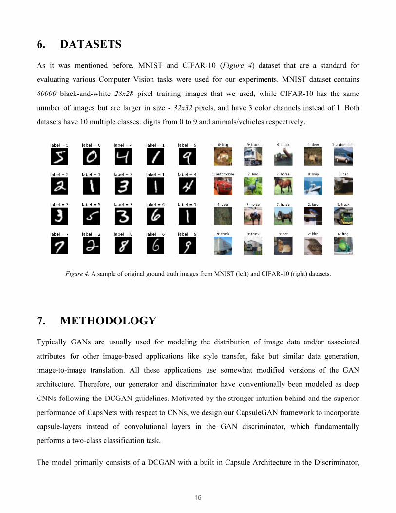
As it was mentioned before, MNIST and CIFAR-10 (Figure 4) dataset that are a standard for

evaluating various Computer Vision tasks were used for our experiments. MNIST dataset contains

60000 black-and-white 28x28 pixel training images that we used, while CIFAR-10 has the same

number of images but are larger in size - 32x32 pixels, and have 3 color channels instead of 1. Both

datasets have 10 multiple classes: digits from 0 to 9 and animals/vehicles respectively.

Figure 4. A sample of original ground truth images from MNIST (left) and CIFAR-10 (right) datasets.

7. METHODOLOGY

Typically GANs are usually used for modeling the distribution of image data and/or associated

attributes for other image-based applications like style transfer, fake but similar data generation,

image-to-image translation. All these applications use somewhat modified versions of the GAN

architecture. Therefore, our generator and discriminator have conventionally been modeled as deep

CNNs following the DCGAN guidelines. Motivated by the stronger intuition behind and the superior

performance of CapsNets with respect to CNNs, we design our CapsuleGAN framework to incorporate

capsule-layers instead of convolutional layers in the GAN discriminator, which fundamentally

performs a two-class classification task.

The model primarily consists of a DCGAN with a built in Capsule Architecture in the Discriminator,

16

that holds a classification function for determining real and fake labels for given images and a

Generator part which has stayed unchanged. We implement our method using the Keras library on top

of TensorFlow and here we fully summarize our experimental settings.

7.1 DISCRIMINATOR STRUCTURE

As we mentioned it earlier, the discriminator comprises only of a Capsule network borrowed from the

original paper with some small additional modifications to it. All the changes are described in this

section.

The model we supply a 28x28 pixel with a single color channel and later 32x32 pixel images with 3

color channels from MNIST and CIFAR-10 datasets respectively as an input. A simple convolutional

layer with 256 filters, 9 pixel kernel size and a stride value of 1 comes as the first layer. This layer

converts pixel intensities to the activities of local feature detectors that are then used as inputs to the

PrimaryCaps. In a lot of modern papers this first layer is often has a large filter size. The reason being

that it allows us to immediately increase the receptive field of all the consecutive layers from now on.

According to the original Dynamic Routing paper, this layer extracts low-level information from the

image and lets us to pass it to the Capsule network. However, different from the paper, we stack

additional Leaky ReLU activation and a batch normalization on top of the first convolutional layer. The

reason for bringing an additional activation function to the initial convolution is to make the

Discriminator perform as well as possible whereas an activation function such as a Leaky ReLU will

not only introduce a non-linearity but will also take care of the vanishing gradient by allowing a small

negative slope [18]:

17

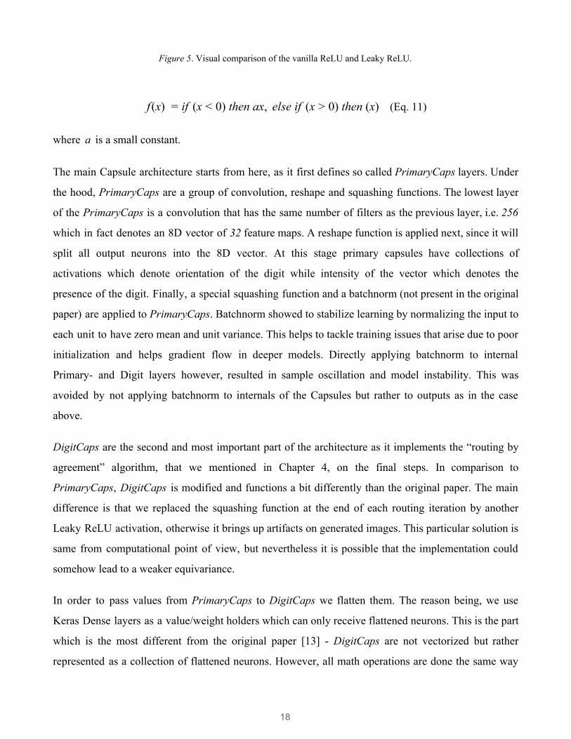
Figure 5. Visual comparison of the vanilla ReLU and Leaky ReLU.

(Eq. 11)(x) f (x ) then ax, else if (x ) then (x) f = i < 0 > 0

where is a small constant.a

The main Capsule architecture starts from here, as it first defines so called PrimaryCaps layers. Under

the hood, PrimaryCaps are a group of convolution, reshape and squashing functions. The lowest layer

of the PrimaryCaps is a convolution that has the same number of filters as the previous layer, i.e. 256

which in fact denotes an 8D vector of 32 feature maps. A reshape function is applied next, since it will

split all output neurons into the 8D vector. At this stage primary capsules have collections of

activations which denote orientation of the digit while intensity of the vector which denotes the

presence of the digit. Finally, a special squashing function and a batchnorm (not present in the original

paper) are applied to PrimaryCaps. Batchnorm showed to stabilize learning by normalizing the input to

each unit to have zero mean and unit variance. This helps to tackle training issues that arise due to poor

initialization and helps gradient flow in deeper models. Directly applying batchnorm to internal

Primary- and Digit layers however, resulted in sample oscillation and model instability. This was

avoided by not applying batchnorm to internals of the Capsules but rather to outputs as in the case

above.

DigitCaps are the second and most important part of the architecture as it implements the “routing by

agreement” algorithm, that we mentioned in Chapter 4, on the final steps. In comparison to

PrimaryCaps, DigitCaps is modified and functions a bit differently than the original paper. The main

difference is that we replaced the squashing function at the end of each routing iteration by another

Leaky ReLU activation, otherwise it brings up artifacts on generated images. This particular solution is

same from computational point of view, but nevertheless it is possible that the implementation could

somehow lead to a weaker equivariance.

In order to pass values from PrimaryCaps to DigitCaps we flatten them. The reason being, we use

Keras Dense layers as a value/weight holders which can only receive flattened neurons. This is the part

which is the most different from the original paper [13] - DigitCaps are not vectorized but rather

represented as a collection of flattened neurons. However, all math operations are done the same way

18

as if they would have been done on vectors.

Flattened neurons get passed into a Keras Dense layer that acts as a prediction vector. The prediction u︿

vector itself consists of 160 neurons denoted as a multiplication of 10 capsules and 16 vectors. We also

set Keras Dense layer parameters such as kernel initializer to He initializer [19] and a bias initializer to

zeros. Next the prediction vector is passed to a 3 length loop where a coupling coefficient which u︿ C

is a softmax over the bias weights of a previous layer (which will make sure that all the capsules in the

layer below sum to one) and . Each multiplication is followed by LeakyReLU activation. The last u︿

layer which determines the realness score of an image in the discriminator is a Keras Dense layer with

a single neuron and a sigmoid.

7.2 GENERATOR STRUCTURE

The generator architecture from DCGAN mainly comprises of deconvolutional layers. The first layer of

the GAN, which takes a uniform noise distribution as input, could be called fully connected as it is Z

just a matrix multiplication, but the result is reshaped into a 2-dimensional tensor and used as the start

of the convolution stack. In our case the noise has a specific length of 100.Z

The second layer that sits on top of the input noise is a fully-connected 8192 neuron layer. It has no

related activation functions but rather acts as representational layer that we will be able later pass

information from. All subsequent layers are groups convolutions, batch norms, ReLU activations and

2D upsamplings. The 2D upsamplings bilinearly repeat the rows and columns in order to increase the

image size.

Obviously our task is to make the Generator output correspond the input size of the Discriminator. For

that the Generator architecture must be able to resize the noise from 8192 back to 28x28 or 32x32

pixels. Finally, we add a tanh activation to the final 32x32x3 convolution in order to produce viable for

a Discriminator results.

19

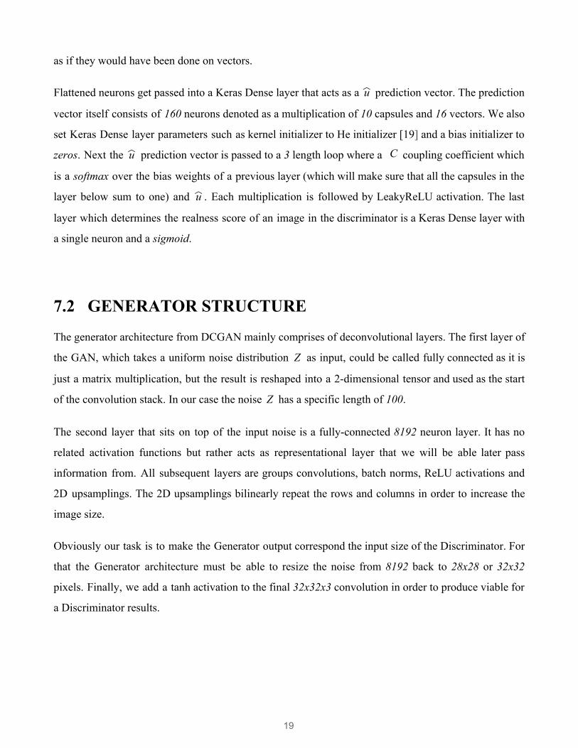
8. RESULTS

Both datasets were trained on a single Nvidia GeForce GTX 660 GPU upon Intel Core i5-7500 CPU

and took about 3 hours for MNIST and 5 hours CIFAR-10 datasets respectively over 30000 epochs.

The epoch quantity was not chosen arbitrarily but rather by visual result convergence. MNIST dataset

results were able to reproduce clearly distinguishable results already from ~ 1000th epoch (which is

excellent, since the original DCGAN achieves this starting from ~ 3000th epoch). Although the same

technique could be applied to CIFAR10 dataset, its output was still not satisfactory after the 20000th

epoch.

Figure 6. A generated example image at 1000th epoch. Digits are still blurred but some are easily recognizable.

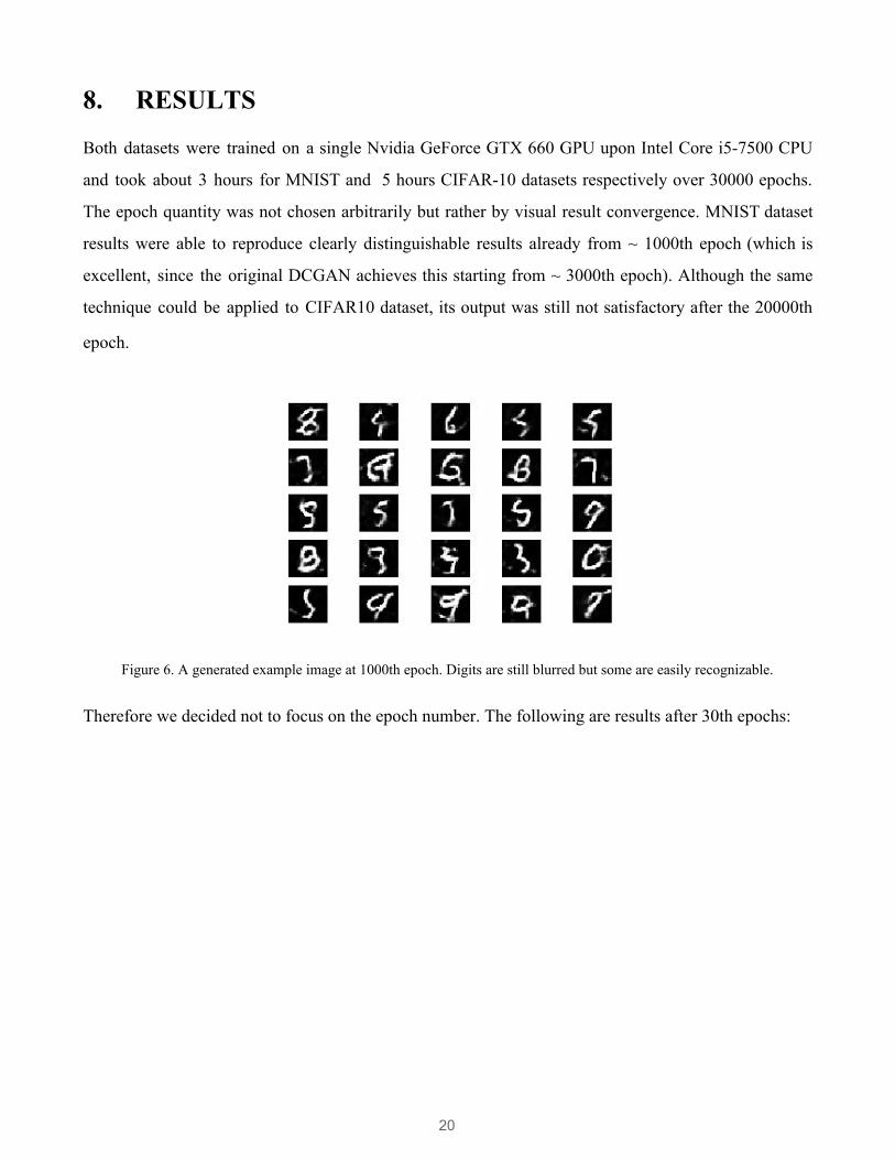
Therefore we decided not to focus on the epoch number. The following are results after 30th epochs:

20

Figure 7. Final outputs at 30000th epoch. a) MNIST sample, top image; b) CIFAR-10 sample, bottom image;

8.1 QUALITATIVE EVALUATION

A problem with generative adversarial models is that there is no clear way to evaluate them

quantitatively. In the past, Goodfellow et al. [17] evaluated GANs by looking at the single nearest

neighbour data from the generated samples. For a better understanding of the quality and realism of

produced images we run an experiment with human evaluators via Amazon Mechanical Turk (AMT).

21

Participants were shown a sequence of 2 image grids at a time and asked to click the most realistic grid

in their opinion. The first grid contained digits from the real ground truth MNIST dataset, whereas

latter contained digits generated by our GAN at 30000th epoch.

The total number of AMT participants used for this task is 1200. According to the AMT reports 63% of

participants were fooled by the produced image. Considering the fact that the shown grids are identical

and the difference between the real and produced grids are hardly visible we conclude that above 50%

result is fairly good (50% would be random guessing). Unfortunately, due to a lack of awareness of

other GAN based AMT experiments conducted on MNIST dataset we are unable to define a

benchmark and make proper comparisons. Furthermore, we do not test CIFAR-10 generated results on

AMT due to low efficiency of them.

8.2 QUANTITATIVE EVALUATION

As we mentioned earlier, unfortunately, GANs losses are very non-intuitive. Mostly it happens due to

the fact that generator and discriminator are competing against each other, hence improvement on the

one means the higher loss on the other. Recent applications of GANs have shown that they are able to

produce excellent samples, however, training GANs often leads to a Nash equilibrium of a non-convex

game with continuous, high-dimensional parameters [20]. Nash equilibrium is a solution concept in

game theory which implies a stable state of a system which involves several players in which no player

can gain by a change of strategy as long as the other player’s strategy remains unchanged. GANs are

typically trained using gradient descent techniques that are designed to find a low value of a cost

function, rather than to find the Nash equilibrium of a game. When used to seek solely for a Nash

equilibrium, these algorithms may fail to converge.

Figure 8 shows losses of the generator while training on MNIST (a) and CIFAR-10 (b) datasets. In the

first case the loss of the model is bouncing around throughout all 30000 epochs although it obviously

decreases over time from 4.0 and flattens at 2.5. It is hard to indicate the flattening since it still

fluctuates a lot, however, the pattern does not seem to leave the boundaries of 2.5 and 1.0 that we

consider as flattening. We assume those fluctuations as a fact that the model is trying to improve itself.

22

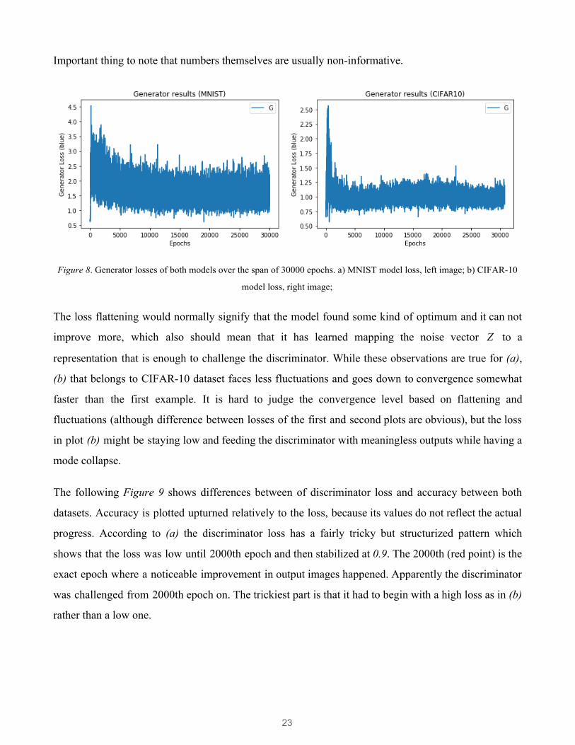
Important thing to note that numbers themselves are usually non-informative.

Figure 8. Generator losses of both models over the span of 30000 epochs. a) MNIST model loss, left image; b) CIFAR-10

model loss, right image;

The loss flattening would normally signify that the model found some kind of optimum and it can not

improve more, which also should mean that it has learned mapping the noise vector to a Z

representation that is enough to challenge the discriminator. While these observations are true for (a),

(b) that belongs to CIFAR-10 dataset faces less fluctuations and goes down to convergence somewhat

faster than the first example. It is hard to judge the convergence level based on flattening and

fluctuations (although difference between losses of the first and second plots are obvious), but the loss

in plot (b) might be staying low and feeding the discriminator with meaningless outputs while having a

mode collapse.

The following Figure 9 shows differences between of discriminator loss and accuracy between both

datasets. Accuracy is plotted upturned relatively to the loss, because its values do not reflect the actual

progress. According to (a) the discriminator loss has a fairly tricky but structurized pattern which

shows that the loss was low until 2000th epoch and then stabilized at 0.9. The 2000th (red point) is the

exact epoch where a noticeable improvement in output images happened. Apparently the discriminator

was challenged from 2000th epoch on. The trickiest part is that it had to begin with a high loss as in (b)

rather than a low one.

23

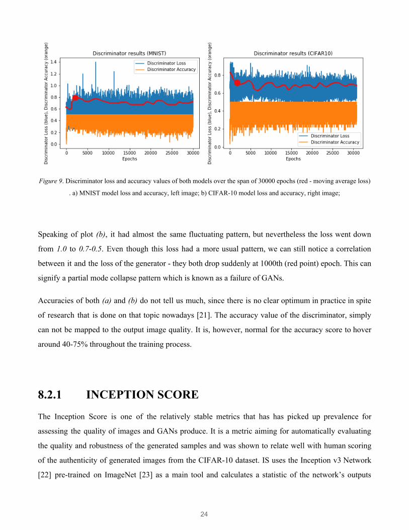
Figure 9. Discriminator loss and accuracy values of both models over the span of 30000 epochs (red - moving average loss)

. a) MNIST model loss and accuracy, left image; b) CIFAR-10 model loss and accuracy, right image;

Speaking of plot (b), it had almost the same fluctuating pattern, but nevertheless the loss went down

from 1.0 to 0.7-0.5. Even though this loss had a more usual pattern, we can still notice a correlation

between it and the loss of the generator - they both drop suddenly at 1000th (red point) epoch. This can

signify a partial mode collapse pattern which is known as a failure of GANs.

Accuracies of both (a) and (b) do not tell us much, since there is no clear optimum in practice in spite

of research that is done on that topic nowadays [21]. The accuracy value of the discriminator, simply

can not be mapped to the output image quality. It is, however, normal for the accuracy score to hover

around 40-75% throughout the training process.

8.2.1 INCEPTION SCORE

The Inception Score is one of the relatively stable metrics that has has picked up prevalence for

assessing the quality of images and GANs produce. It is a metric aiming for automatically evaluating

the quality and robustness of the generated samples and was shown to relate well with human scoring

of the authenticity of generated images from the CIFAR-10 dataset. IS uses the Inception v3 Network

[22] pre-trained on ImageNet [23] as a main tool and calculates a statistic of the network’s outputs

24

when applied to our generated images. IS is defined by the following formula:

(Eq. 12)S (G) xp (ε D (p (y|x) || p (y) )) I = e x∼pg KL

where indicates that is an image sampled from , is the KL divergence between the ∼px g x pg DKL

distributions and , is the conditional class distribution, and is the p q (y|x)p (y) (y|x) p (x)p = ∫

xp g

marginal class distribution. The IS is aimed to expose two desirable qualities of the GAN [12]:

● the Inception Network should be highly confident there is a single object in the image i.e. the

generated images should contain clear objects and should have a low entropy. (y|x)p

● the generator should output diverse sample of images from all the different classes it was

trained on, which means should have a high entropy. (y)p

If both of these traits are met by a GAN well enough, then we expect a large KL divergence between

the distributions and , resulting in a large score. (y)p (y|x)p

Since the Inception Network is pre-trained on ImageNet dataset and takes 3 channel images as an input,

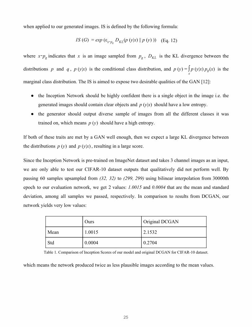
we are only able to test our CIFAR-10 dataset outputs that qualitatively did not perform well. By

passing 60 samples upsampled from (32, 32) to (299, 299) using bilinear interpolation from 30000th

epoch to our evaluation network, we get 2 values: 1.0015 and 0.0004 that are the mean and standard

deviation, among all samples we passed, respectively. In comparison to results from DCGAN, our

network yields very low values:

Ours Original DCGAN

Mean 1.0015 2.1532

Std 0.0004 0.2704

Table 1. Comparison of Inception Scores of our model and original DCGAN for CIFAR-10 dataset.

which means the network produced twice as less plausible images according to the mean values.

25

9. DISCUSSION

GANs are never easy to train. The fact that we have 2 separate networks having a battle with each

other, we are in a need to optimize them both so that the battle lasts as long as possible by not

privileging one of them. Even with a different Discriminator architecture such as Capsules, it still does

not resolve the inner GAN issues, but instead addresses issues related to Convolutions.

To sum up the results we have, in the case of MNIST images we are able to clearly see digits and they

are identical to the source distribution. This signifies a successful training process and we claim the

results plausible after the AMT evaluations.

On the other hand, we can not claim the same for outputs for CIFAR-10 dataset. We observed visual

mistakes as well as an extremely low Inception Score. The network did not manage to paint objects as a

whole, but rather gave up in the middle of the process leading to blurry spots looking like objects but

not quite. Although we already mentioned that the reason could be a partial mode collapse, it is hard to

prove it since it can be triggered in a completely random fashion, making it very difficult to interpret

and debug. But what is the mode collapse and how to handle it? Imagine our source distribution has

several peaks, i.e. several common patterns which in our case are animals and vehicles. The generator

learns that it can fool the discriminator by producing values close to only the first class which leads to

different kinds of artifacts or just producing images of one similar type. However, since in our case

images look quite different from each other, it is possible that the problem is in the Capsule architecture

itself and it can not discriminate well enough.

By the time this paper is being written, the code repository (see Appendices) has 40 GitHub stars which

show others’ appreciation to the work and are used for ranking. The repository also has 12 forks which

indicate how many users are currently on continuation of our work and are able to submit Pull

Requests, in other words collaborate and send updates.

10. FURTHER RESEARCH

There is a huge space where GANs can be applied and there is still so much to research about them. In

particular GANs have made a lot of progress in Computer Vision recently: image inpainting, style

26

transfer, image enhancement and etc. Nevertheless, new papers and improvements to existing models

are being released almost every week.

Since our paper is about changing the architecture of a GAN and incorporating Capsules into it, it can

be considered as a model improvement taking into account discoveries in Convolutional Neural

Networks in general. Some of the ideas for further research for this topic are: integrating the original

loss function from S. Sabour et al. [13] and trying to make them work with bigger datasets such as

CIFAR-100.

11. CONCLUSION

In conclusion, we described the existing bottlenecks of CNNs for modern Computer Vision tasks and

gave a deep explanation of Capsule Networks, its separate layers and the main Routing algorithm

behind it. Then we illustrated and listed the properties of the model that we got after incorporating

Capsules into a vanilla DCGAN. Results and experiments including AMT and Inception Score showed

that the incorporating task was successful when training on the first MNIST dataset but failed on

CIFAR-10, which brings us to conclusion that GANs and Capsules are powerful but not yet stable

when combined.

27

REFERENCES

1. Generative Models. OpenAI. Blog. June 2016. Web link: https://blog.openai.com/generative-models/

2. Jonathan Hui. Understanding Dynamic Routing between Capsules (Capsule Networks). Blog. Nov.

2017. Web link: https://jhui.github.io/2017/11/03/Dynamic-Routing-Between-Capsules

3. Max Pechyonkin. Understanding Hinton’s Capsule Networks. Part I: Intuition. Medium blog. Nov.

2017. Web link:

https://medium.com/ai%C2%B3-theory-practice-business/understanding-hintons-capsule-networks-part-i-intuiti

on-b4b559d1159b

4. Sammer Puran. Will Capsule Networks replace Neural Networks? Quora question. Dec. 2017. Web

link: https://www.quora.com/Will-capsule-networks-replace-neural-networks

5. Alec Radford, Luke Metz, Soumith Chintala. Unsupervised Representation Learning with Deep

Convolutional Generative Adversarial Networks. indico Research, Facebook AI Research. Jan. 2016.

6. David Berthelot, Thomas Schumm, Luke Metz. BEGAN: Boundary Equilibrium Generative

Adversarial Networks. Google. May 2017.

7. Martin Arjovsky, Soumith Chintala, Léon Bottou. Wasserstein GAN. Courant Institute of

Mathematical Sciences, Facebook AI Research. Dec. 2017.

8. Quan Hoang, Tu Dinh Nguyen, Trung Le, Dinh Phung. Multi-Generator Generative Adversarial

Nets. University of Massachusetts-Amherst, PRaDA Centre, Deakin University. Oct. 2017.

9. Chongxuan Li, Kun Xu, Jun Zhu, Bo Zhang. Triple Generative Adversarial Nets. Dept. of Comp.

Sci. & Tech., TNList Lab, State Key Lab of Intell. Tech. & Sys., Center for Bio-Inspired Computing

Research, Tsinghua University. Nov. 2017.

10. Ayush Jaiswal, Wael AbdAlmageed, Yue Wu, Premkumar Natarajan. CapsuleGAN: Generative

Adversarial Capsule Network. USC Information Sciences Institute. Mar. 2018.

11. Daniel Jiwoong Im, Roland Memisevic, Chris Dongjoo Kim, Hui Jiang. Generative Adversarial

28

Metric. Montreal Institute for Learning Algorithms, Department of Engineering and Computer Science.

2016.

12. Zhiming Zhou, Weinan Zhang, Jun Wang. Inception Score, Label Smoothing, Gradient Vanishing

and -log(D(x)) Alternative. Shanghai Jiao Tong University. Aug. 2017.

13. Sara Sabour, Nicholas Frosst, Geoffrey E. Hinton. Dynamic Routing Between Capsules. Google

Brain. Nov. 2017.

14. G. E. Hinton, A. Krizhevsky, S. D. Wang. Transforming Auto-encoders. Department of Computer

Science, University of Toronto. 2011.

15. Max Pechyonkin. Understanding Hinton’s Capsule Networks. Understanding Hinton’s Capsule

Networks. Part II: How Capsules Work. Nov. 2017. Web link:

https://medium.com/ai%C2%B3-theory-practice-business/understanding-hintons-capsule-networks-part-ii-how-c

apsules-work-153b6ade9f66

16. Jonathan Hui. Understanding Matrix capsules with EM Routing. Blog. Nov. 2017. Web link:

https://jhui.github.io/2017/11/14/Matrix-Capsules-with-EM-routing-Capsule-Network/

17. Ian J. Goodfellow, Jean Pouget-Abadie, Mehdi Mirza, Bing Xu, David Warde-Farley, Sherjil Ozair,

Aaron Courville, Yoshua Bengio. Generative Adversarial Networks. Departement d’informatique et de

recherche op ´ erationnelle. June 2014.

18. Andrej Karpaty. CS231n Convolutional Neural Networks for Visual Recognition course. Stanford

University. 2017.

19. Kaiming He, Xiangyu Zhang, Shaoqing Ren, Jian Sun. Delving Deep into Rectifiers: Surpassing

Human-Level Performance on ImageNet Classification. Microsoft Research. Feb. 2016.

20. Tim Salimans, Ian Goodfellow, Wojciech Zaremba, Vicki Cheung, Alec Radford, Xi Chen.

Improved Techniques for Training GANs. OpenAI. June 2016.

21. Martin Arjovsky, Leon Bottou. Towards Principled Methods for Training Generative Adversarial

Networks. Courant Institute of Mathematical Sciences, Facebook AI Research. Jan 2017.

29

22. Christian Szegedy, Vincent Vanhoucke, Sergey Ioffe, Jonathon Shlens, Zbigniew Wojna.

Rethinking the Inception Architecture for Computer Vision. Google Inc., University College London.

Dec. 2015.

23. ImageNet. Visual database designed for use in visual object recognition software research.

Stanford Vision Lab, Stanford University, Princeton University. 2012.

30

APPENDICES

Follow the link to see the project repository: https://github.com/gusgad/capsule-GAN. The main code

for the paper is within a Jupyter Notebook called “capsule_gan.ipynb” and written in Python language.

31