Embed Size (px)
Citation preview
Discrete Applied Mathematics 137 (2004) 311–341www.elsevier.com/locate/dam
Cardinality constrained minimum cut problems:complexity and algorithms
Maurizio Bruglieria ;1 , Francesco Ma*olia , Matthias EhrgottbaDipartimento di Elettronica e Informazione, Politecnico di Milano, Piazza Leonardo da Vinci 32,
20133 Milano, ItalybDepartment of Engineering Science, University of Auckland, Private Bag 92019, Auckland,
New Zealand
Received 27 March 2002; received in revised form 23 May 2003; accepted 26 May 2003
Abstract
In several applications the solutions of combinatorial optimization problems (COP) are re-quired to satisfy an additional cardinality constraint, that is to contain a 3xed number of elements.So far the family of (COP) with cardinality constraints has been little investigated. The presentwork tackles a new problem of this class: the k-cardinality minimum cut problem (k-card cut).For a number of variants of this problem we show complexity results in the most signi3cantgraph classes. Moreover, we develop several heuristic algorithms for the k-card cut problem forcomplete, complete bipartite, and general graphs. Lower bounds are obtained through an SDPformulation, and used to show the quality of the heuristics. Finally, we present a randomizedSDP heuristic and numerical results.? 2003 Elsevier B.V. All rights reserved.
Keywords: Cut problems; k-cardinality minimum cut; Cardinality constrained combinatorial optimization;Computational complexity; Semide3nite programming
1. Introduction
In recent years a number of papers have been published in which classical combina-torial optimization problems have been modi3ed by imposing an additional cardinality
1 The work of M.B. has been supported by Ph.D. MA.C.R.O. Grant of the Department of Mathematics“F. Enriquez”, University of Milan.
E-mail addresses: [email protected] (M. Bruglieri), ma*[email protected] (F. Ma*oli),[email protected] (M. Ehrgott).
0166-218X/$ - see front matter ? 2003 Elsevier B.V. All rights reserved.doi:10.1016/S0166-218X(03)00358-5
312 M. Bruglieri et al. / Discrete Applied Mathematics 137 (2004) 311–341
constraint, i.e. feasible solutions were constrained to contain a given number k of ele-ments. Applications of cardinality constrained tree problems are in oil-3eld leasing [12]and facilities layout [14]. [8] deals with portfolio optimization, when the portfolio hasto contain a 3xed number of assets. A number of other problems, e.g. the assignmentproblem [10], have also been studied under cardinality constraints. A survey on thetopic with extensive references is available [13]. A class of combinatorial optimizationproblems which have applications in a wide variety of areas are cut problems, i.e. theproblems to 3nd in a given graph a cut of maximal (or minimal) weight. In physics,for example, the maximum cut problem models the problem of 3nding a ground stateof spin glasses having zero magnetization. In VLSI design, it models the problem ofminimizing the number of vias (holes on a printed circuit board, or contacts on achip), see [3]. In numerical analysis it is helpful in 3nding the L-U factorization of thematrix of a linear system. The minimum cut problem has applications for example innetwork reliability theory and in compilers for parallel languages. For some of those,the addition of a cardinality constrained might be desirable. With this motivation weset out to investigate k cardinality cut problems. This paper contains the results of ourresearch which has been also the subject of the 3rst author’s Ph.D. thesis (see [5]). Westart with some basic de3nitions. Let G = (V; E) be an undirected graph with vertexset V and edge set E.
De�nition 1.
1. A cut is a partition of vertex set V in two sets V1; V2 called the shores of thecut. A cut edge set C := {{v1; v2} ∈E : v1 ∈V1; v2 ∈V2} is associated with everycut.
2. Given s; t ∈V an s-t cut is a cut (V1; V2) such that s∈V1 and t ∈V2.
Since from the cut edge set C one can easily reconstruct the shores V1; V2, inthe sequel we shall indiJerently de3ne cuts either through the shores or throughthe cut edge set. Let us introduce the notation �(A; B) and �(A) for A; B ⊂ V asfollows:
�(A; B) := {{v1; v2} ∈E : v1 ∈A; v2 ∈B};�(A) := �(A; KA);
where KA denotes V \A. Let w : E → N be a non-negative integer function on the edgeset of graph G. The minimum cut problem (min cut) and the maximum cut problem(max cut) are the problems to 3nd a cut such that the sum of the weights of the cutedge set C is minimal and maximal, respectively. It will be convenient, to denote theweight of any subset of edges F ⊂ E by
w(F) :=∑e∈F
w(e):
We can now introduce cardinality constrained cut problems. Let k be a positiveinteger.
M. Bruglieri et al. / Discrete Applied Mathematics 137 (2004) 311–341 313
b
1 100
ca
d e
1001
1
10
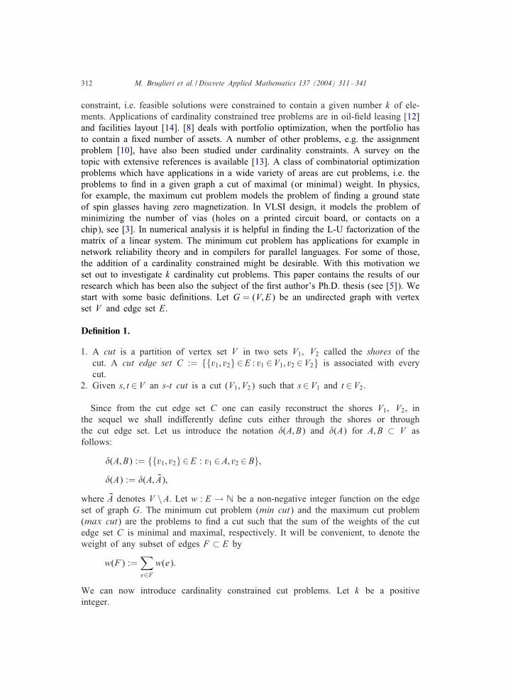
Fig. 1. Illustrating diJerent cardinality constraints.
De�nition 2.
1. The k-cardinality minimum cut problem k-card cut is the problem to 3nd a cutsuch that cut edge set C has cardinality k and the sum of the weights of the edgesbelonging to C is minimal.
2. The k-cardinality minimum s-t cut problem k-card s-t cut is de3ned analogously tok-card cut with the additional request that the cut we want to 3nd is an s-t cut.
3. The ¿ k-card cut and ¿ k-card s-t cut problems are de3ned analogously to k-cardcut and k-card s-t cut only that the cardinality of C is required to be greater thanor equal to k.
From the de3nitions we can make some observations. The simple example given inFig. 1 shows that k-card cut and ¿ k-card cut can have diJerent optimal solutions.Indeed, V ∗
1 ={b} is an optimal solution for k-card cut with value 101, whereas V ′1={a}
is an optimal solution for ¿ k-card cut with value 3, when k = 2.However, we immediately have some relations between k-card cut and ¿ k-card cut.
Clearly, the optimal value of ¿ k-card cut is always less than or equal to the optimalvalue of k-card cut. Furthermore, for every graph class for which k-card cut is easy¿ k-card cut is easy, too, because it can be solved taking the best solution of p-cardcut with p=k; k+1; : : : ; |E|, respectively. It is important to note that without cardinalityconstraints the problems of De3nition 2 are all easy to solve, because they becomeminimal cut problems and several e*cient algorithms exist in the literature for solvingthe latter (see [22,27,31]). The example above shows that the situation is quite diJerentdue to the cardinality constraint. In Section 2 below we shall present complexity resultsfor a number of important graph classes. The rest of the paper is organized as follows.In Section 3 we present three heuristics for complete and complete bipartite graphs.A heuristic for general graphs which is not guaranteed to 3nd a cut of the desiredcardinality (this problem is shown to be NP-complete in Section 2) is also given.Section 4 presents lower bounds based on LP relaxation and SDP relaxation. In Section5 a randomized SDP heuristic is given, for which we can prove lower and upper boundson the deviation of expected cardinality from the desired k and of the weight of thecut from optimality.
314 M. Bruglieri et al. / Discrete Applied Mathematics 137 (2004) 311–341
2. Complexity of cardinality constrained minimum cut problems
In this section we prove some results on computational complexity of cardinalityconstrained cut problems. First, we shall prove NP-hardness on general graphs. Wethen proceed to complete and complete bipartite graphs, for which NP-hardness stillholds. Further results are about trees, grid graphs, and planar graphs, for which ourproblems are polynomially, respectively randomized polynomially solvable.
2.1. General graphs
Our 3rst result shows that even 3nding a feasible solution is NP-hard.
Theorem 1. k-card cut and k-card s-t cut are strongly NP-hard even if w(e)=1 forall e∈E.
Proof. We prove the result for k-card cut 3rst. It is easy to see that the recognitionversion of k-card cut belongs to NP. For proving the strong hardness we polynomiallyreduce simple max cut to k-card cut. An instance of simple max cut is an undirectedgraph G = (V; E) where we look for a cut with the maximum number of edges. Wecan transform this instance into instances for k-card cut considering the same graphwith weight w(e) = 1 for all e∈E and values of k between 1 and |E|. A solution ofk-card cut for the maximum feasible value of k is also a solution of simple max cut.The proof follows from strong NP-hardness of simple max cut (see [17, p. 210]).Solving k-card s-t cut for all pairs of vertices s; t and taking the best solution we obtaina solution for k-card cut. Hence k-card s-t cut is also strongly NP-hard.
The proof of Theorem 1 is not valid for classes of graphs (e.g. planar graphs) forwhich simple max cut belongs to P (see [9, p. 247]). The case of planar graphs isdiscussed in Section 2.6.Analogously to Theorem 1 we can proveNP-hardness of¿ k-card cut and¿ k-card
s-t cut.
Proposition 1. The ¿ k-card cut and ¿ k-card s-t cut problems are strongly NP-hard, even if w(e) = 1 for all e∈E.
2.2. Complete graphs
For complete graphs all possible cardinalities of cuts can be described.
Lemma 1. If G= (V; E) with |V |= n is a simple and complete graph k-card cut andk-card s-t cut are feasible if and only if
k = j(n− j) with j∈{1; : : : ;
⌊n2
⌋}: (1)
M. Bruglieri et al. / Discrete Applied Mathematics 137 (2004) 311–341 315
Proof. Due to completeness of G, every partition of V into V1 and V2 with |V1| =j6 n=26 n− j = |V2| de3nes a cut with k = j(n− j) edges.
Thus, solving (1) with given k for j, we have that k-card cut and k-card s-t cut areinfeasible, if and only if � := n2 − 4k ¡ 0 or if (n− √
�)=2 is not integer. Thereforewe have:
Proposition 2. If G is a simple and complete graph and w(e) = 1 for all e∈E thenboth k-card cut and k-card s-t cut are in P.
As a consequence of Lemma 1, on complete graphs, the k-card cut problem isequivalent to the bisection problem, i.e. to 3nd a minimal cut with 3xed cardinalityshores. The latter problem is well known in the literature (see [1,9, pp. 256–259]).Although Lemma 1 establishes that for a complete graph the cardinalities of all possiblecuts can be determined in polynomial time, we have that the number of all feasiblek-cardinality cuts is exponential in the size of the problem for each value of k. Indeed,if j represents the cardinality of the minimal shore as in the proof of Lemma 1, allpossible k-cardinality cuts are given by all choices of j elements of V . Thus the numberof all possible k-cardinality cuts is ( nj )¿ 2j. We will prove in Proposition 3 that forcomplete graphs with non-uniform weights on the edges k-card cut is strongly NP-hard.To prove NP-hardness of the weighted problems, we use a reduction of the equicutproblem. This is to 3nd a cut with shores of size n=2 and �n=2 which has minimalweight.
Lemma 2. If G is a simple complete graph with non-uniform weights on the edgesthe equicut problem is strongly NP-hard.
Proof. The equicut problem is strongly NP-hard for general graphs as proved in [18].Now we will reduce the equicut problem for general graphs to the equicut problemfor complete graphs. Given a graph G = (V; E), |V | = n, with edge-weight functionw : E → N we transform it into a complete graph G′ = (V; E′) adding the lackingedges. On the new graph G′ we consider the edge-weight function w′ : E′ → Nde3ned for all e∈E′ in the following way:
w′(e) =
{w(e) + 1 ∀e∈E1 ∀e∈E′ \ E:
Since the total weight of each equicut in G′ diJers from the total weight of the cor-responding equicut in the original graph by the 3xed amount c= n=2�n=2 we havethat an optimal equicut in the original general graph corresponds to an optimal equicutin the new (complete) graph.
Proposition 3. If G is a simple complete graph with non-uniform weights on the edgesthen both k-card cut and k-card s-t cut are strongly NP-hard.
316 M. Bruglieri et al. / Discrete Applied Mathematics 137 (2004) 311–341
Proof. Reduction from equicut. Given an instance of equicut we can solve it solvingthe k-card cut problem with k = n=2�n=2 . The strong hardness derives from thestrong hardness of equicut for complete graphs established by Lemma 2. For provingthe strong hardness of k-card s-t cut we can reduce k-card cut to k-card s-t cut likein the proof of Theorem 1.
We now proceed to show NP-hardness for ¿ k-card cut for which we introduce thefollowing problem. Given an edge-weighted graph G = (V; E) and a positive integerb∈ [|V |=2; |V |] the min cut into bounded sets problem is the problem of 3nding apartition of V into disjoint sets V1 and V2 such that |V1|6 b, |V2|6 b and such thatthe sum of the weights of the edges between V1 and V2 is minimal.
Lemma 3. If G = (V; E) is a complete graph with non-uniform edge weights the mincut into bounded sets problem for G is strongly NP-hard.
Proof. The min cut into bounded sets problem is strongly NP-hard for general graphsas proved in [18]. For proving that the problem remains stronglyNP-hard for completegraphs, too, we can reduce the general graph case to the complete graph case like inthe proof of Lemma 2.
Proposition 4. If G= (V; E) is a simple complete graph with non-uniform weights onthe edges ¿ k-card cut is strongly NP-hard.
Proof. Reduction from the min cut into bounded sets problem. Due to completenessof G, a shore S of a ¿ k-card cut with k = b(n− b) is such that
|S|(n− |S|)¿ b(n− b): (2)
Therefore, solving (2) with given b for |S|, we have n− b6 |S|6 b and since |S| =n−| KS| from n−b6 |S| it follows that | KS|6 b, too. Hence the strong hardness derivesfrom the strong hardness of the min cut into bounded sets for complete graphs provedin Lemma 3.
2.3. Complete bipartite graphs
For a complete bipartite graph Kn;m we shall denote the partition of the vertex setV = L∪R and assume |L|= n1; |R|= n2 so that |E|= n1n2: The vertex sets are writtenas L= {l1; : : : ; ln1} and R= {r1; : : : ; rn2}. As for complete graphs, we can characterizethe cardinalities of possible cuts.
Lemma 4. Given a complete bipartite graph Kn1 ;n2 = (L∪R; E), k-card cut and k-cards-t cut are feasible if and only if
k = jn1 + in2 − 2ij (3)
with j∈ {0; 1; : : : ; n2}; i∈ {0; 1; : : : ; n1}; and i + j6 (n1 + n2)=2.
M. Bruglieri et al. / Discrete Applied Mathematics 137 (2004) 311–341 317
Proof. Let the vertex set S be a shore of a cut. We can suppose |S|6 (n1 + n2)=2because otherwise KS is so and it determines the same cut. Let i= |S∩L| and j= |S∩R|,thus i is an integer between 0 and |L|= n1, j is an integer between 0 and |R|= n2 andi + j = |S|. Therefore
�(S) = �(S ∩ L) ∪ �(S ∩ R) \ �(S ∩ L; S ∩ R)and
|�(S)| = |�(S ∩ L)| + |�(S ∩ R)| − 2|�(S ∩ L; S ∩ R)| = jn1 + in2 − 2ij:
In this way the cardinalities of all possible cuts are given by (3).
Given a k value we can have several pairs of values i; j satisfying (3). For examplefor the graph K3;2 both i= j=1 and i=1; j=0 satisfy (3) for k=3. Moreover, unlikefor complete graphs there is no one to one correspondence between the cardinality k ofthe cut and the cardinality of the minimal shore S of the cut. S1={r2} and S2={l3; r1}determine both cuts with cardinality k =3. Analogously, it is easy to see that two cutswith diJerent cardinalities can have minimal shores of the same cardinality.
Proposition 5. Given a complete bipartite graph Kn1 ;n2 = (V; E) such that w(e)=1 forall e∈E, both k-card cut and k-card s-t cut are polynomially solvable.
Proof. Through formula (3) we can check feasibility in polynomial time. If the problemis feasible, any choice of j vertices of L and of i vertices of R de3nes a solution fork-card cut. For k-card s-t cut we distinguish two cases:
• Vertices s and t both belong to L (or R) Then if every pair of values i; j satisfying (3)for the given value of k has j=0 or j=n1 then the problem is infeasible. Otherwisesuppose i; j satisfy (3) with j between 1 and n1 − 1. In this case a solution S isgiven by {s} union any choice of j − 1 vertices of L \ {s; t} union any choice of ivertices of R.
• Vertex s belongs to L and vertex t belongs to R. Let i; j be a pair of values satisfying(3) for the given value of k. We distinguish three subcases:◦ If i6 n2 − 1 and j �= 0, a solution S is given by {s} union any choice of j − 1vertices of L \ {s} union any choice of i vertices of R \ {t}:
◦ If i6 n2 − 1 and j = 0, S is given by {t} union any choice of i − 1 vertices ofR \ {t}.
◦ Finally, if i = n2, S is given by R union any choice of j vertices of L \ {s}.
This completes the construction of an s-t k-card cut.
Proposition 6. Given a complete bipartite graph Kn1 ;n2 = (V; E) with non-uniformedge-weights, both k-card cut and k-card s-t cut are strongly NP-hard.
Proof. We reduce the k-card cut problem for complete graphs to the k-card cut problemfor complete bipartite graphs. Given the edge-weighted complete graph Kn = (V; E)
318 M. Bruglieri et al. / Discrete Applied Mathematics 137 (2004) 311–341
with V = {v1; : : : ; vn} and weight function w : E → N let us create the edge-weightedcomplete bipartite graph Kn;n = (L ∪ R; E′) with L = {v1; : : : ; vn}, R = {v′1; : : : ; v′n} andweight function w′ : E′ → N de3ned for all e∈E′ in the following way:
w′(e) =
{w({vi; vj}) if e = {vi; v′j} with i �= j;
M if e = {vi; v′i};
where M ¿ 2∑
e∈E w(e). We observe that if k is the cardinality of a cut for Kngenerated by the vertex set S with |S| = j, then 2k is the cardinality of a cut forKn;n. Indeed it is easy to check through formulas (1) and (3) that the cut generatedin Kn;n by any vertex set S ′ such that |S ′ ∩ L| = |S ′ ∩ R| = j has cardinality 2k.Moreover, we observe that the weight of the optimal 2k-card cut is less than Mbecause �({v1; : : : ; vj; v′1; : : : ; v′j}) is a 2k-card cut having weight less than M . For thisreason an optimal 2k-card cut cannot contain any edge e of the form e= {vi; v′i}. Thusfor every shore S ′ of an optimal 2k-card cut vi ∈ S ′ if and only if v′i ∈ S ′. Thereforethe minimal shore of an optimal 2k-card cut for Kn;n is of the form
S ′ = {vh1 ; : : : ; vhj ; v′h1 ; : : : ; v′hj}
with j satisfying j(n − j) = k. Now we want to show that S = {vh1 ; : : : ; vhj} is anoptimal k-card cut for Kn. If S is not optimal then there exists S = {vp1 ; : : : ; vpj} such
that w(�(S))¡w(�(S)). But in this way S′= S ∪ {v′p1
; : : : ; v′pj} de3nes a 2k-card cutfor Kn;n such that
w′(�(S′)) =
∑u∈S′∩L
∑v∈R\(S′∩R)
w′({u; v}) +∑
u∈L\(S′∩L)
∑v∈S′∩R
w′({u; v})
= 2∑
u∈S′∩L
∑v∈L\(S′∩L)
w({u; v})
= 2w(�(S))¡ 2w(�(S)) = w′(�(S ′))
and this contradicts the optimality of S ′. Hence the strong hardness of k-card cut forcomplete bipartite graphs follows from the strong hardness of k-card cut for completegraphs proved in Proposition 3. For proving the strong hardness of k-card s-t cut wecan reduce k-card cut to k-card s-t cut like in the proof of Theorem 1.
Proposition 7. Given a complete bipartite graph Kn1 ;n2 = (V; E) with non-uniformedge-weights, both ¿ k-card cut and ¿ k-card s-t cut are strongly NP-hard.
Proof. We can reduce the ¿ k-card cut problem for complete graphs to the ¿ k-cardcut problem for complete bipartite graphs like in the proof of Proposition 6. In thisway the validity of the proposition follows from the strong hardness of ¿ k-card cutfor complete graphs proved in Proposition 4.
M. Bruglieri et al. / Discrete Applied Mathematics 137 (2004) 311–341 319
2.4. Trees
We shall show that cut problems on trees remain very easy, even withcardinality constraints. The basis of our results is a characterization of cuts provedin [26].
Lemma 5. For a graph G, C ⊂ E is the edge set of a cut if and only if C has aneven number (possibly zero) of edges in common with any cycle of G.
Proposition 8. When G is a tree, k-card cut is in P.
Proof. Since G is a tree, it has no cycle. So from Lemma 5 any choice of k edges isa k-card cut. Therefore in this case the k edges with smallest weight are a solution ofk-card cut.
To establish the result for s-t cuts we use the following lemma.
Lemma 6. Let G=(V; E) be a tree and s; t ∈V then every s-t cut has an odd numberof edges in common with the path between vertex s and vertex t.
Proof. Let P be the path between vertex s and vertex t (the existence and uniquenessof the path is ensured from G being a tree). Let V1; V2 be the shores of an s-t cutand let C be the edge set. It is easy to see that shores V1 and V2 de3ne in the graphG′ = (V; E ∪ {s; t}) a cut having cut edge set C′ = C ∪ {s; t}. Applying Lemma 6 tocycle P ∪ {s; t} of graph G′ it follows that the cardinality of C ∩ P must be odd.
Proposition 9. When G is a tree, k-card s-t cut belongs to P.
Proof. Let P be the path between the vertex s and the vertex t. By Lemma 6 everys-t cut has an odd number of edges in common with P. Let F be the set of the ksmallest weight edges in G. If |P ∩ F | is odd then the edge set C = F is an optimalsolution of k-card s-t cut. Else if |P ∩ F | is even we obtain C from F modifying Fas little as possible to have |P ∩ C| odd. There are the following four cases.
1. If P\F=∅, let e∗ ∈P and e∈ KF be such that w(e∗)=maxe∈Pw(e); w(e)=mine∈ KFw(e);respectively. An optimal solution is given by C = F \ {e∗} ∪ {e}.
2. If F \ P = ∅, let e∗ ∈F and e∈ KP be such that w(e∗) = maxe∈F w(e); w(e) =mine∈ KP w(e); respectively. An optimal solution is given by C = F \ {e∗} ∪ {e}.
3. If P ∩ F = ∅, let e∗ ∈F and e∈P be such that w(e∗) = maxe∈F w(e); w(e) =mine∈P w(e); respectively. An optimal solution is given by C = F \ {e∗} ∪ {e}.
4. In any other case let e∗; e; e; and Ke be such that w(e∗) = mine∈P\F w(e); w(e) =mine∈(P∪F)w(e); w(e) = maxe∈F\P w(e); and w( Ke) = maxe∈P∩F w(e); respectively.If (P ∪ F) �= ∅ then it easy to see that if w(e∗) − w(e)6w(e) − w( Ke) an optimalsolution is given by C =F \ {e} ∪ {e∗}, otherwise it is given by C =F \ { Ke} ∪ {e}.If (P ∪ F) = ∅ an optimal solution is C = F \ {e} ∪ {e∗}.
320 M. Bruglieri et al. / Discrete Applied Mathematics 137 (2004) 311–341
2.5. Grid graphs
De�nition 3. A simple grid graph is a graph G = (V; E) with (h + 1)(l + 1) verticesarranged in l+1 horizontal rows and h+1 columns, and edges connecting vertices inadjacent rows (columns) vertically (horizontally). The horizontal and vertical lengthsof G are h and l, respectively. Let vi; j be the vertex at row i and column j in G fori = 0; 1; : : : ; l, j = 0; 1; : : : ; h.
Our results for grid graphs show that with the exception of k = 1 and k = n2 − 2cuts with cardinality k always exist. The complexity follows from the results we proveabout planar graphs in Section 2.6.
Lemma 7. If G = (V; E) is a simple grid graph it has a cut of cardinality m, wherem= |E|.
Proof. Let h and l be the horizontal length and vertical length of G and let vi; j be asde3ned in De3nition 3. It is easy to see that the set T de3ned as
T := {vi; j ∈V : 06 i6 l; 06 j6 h; i; j both even or i; j both odd}
generates a cut with edge set equal to E.
Lemma 8. If G = (V; E) is a simple grid graph vertex set T de=ned in Lemma 7has �(h − 1)(l − 1)=2 vertices of degree 4 and h + l vertices of degree 2 or 3. Inparticular it has 4 vertices of degree 2 if h and l are both even and it has 2 verticesof degree 2 in any other case.
The proof of Lemma 8 is omitted since it is trivial.
Proposition 10. If G = (V; E) with |E| = m is a simple grid graph k-card cut andk-card s-t cut are feasible if and only if
k = 2; 3; : : : ; m− 2; m: (4)
Proof. Let us suppose h¿ 3 and l¿ 1 (or vice versa) otherwise the Proposition istrivial. Let T and P be the vertex sets de3ned in the proofs of Lemma 7 and Lemma8. Let S denote the smaller shore of a cut. If k6 4�(h− 1)(l− 1)=2 we set S ′ equalto p= k=4 vertices of P including vertex v1;1 and
S := S ′ ∪ {v0;2} if k − 4p= 3;
S := S ′ ∪ {v0;0} if k − 4p= 2;
S := S ′ \ {v1;1} ∪ {v0;0; v0;2} if k − 4p= 1;
S := S ′ if k − 4p= 0:
M. Bruglieri et al. / Discrete Applied Mathematics 137 (2004) 311–341 321
If 4�(h− 1)(l− 1)=2 ¡k6m− d where
d=
{8 if h; l both even;
4 otherwise
we set S ′ := P, we add to S ′ q vertices of the set
Q := {vi; j ∈V : i = 0; l; 16 j6 h− 1; i; j both even or i; j both odd}including vertex v0;2, with
q :=⌊k − 4p∗
3
⌋; p∗ :=
⌈(h− 1)(l− 1)
2
⌉
and we set
S := S ′ ∪ {v0;0} if k − 4p∗ − 3q= 2;
S := S ′ \ {v0;2} ∪ {v0;0; v} if k − 4p∗ − 3q= 1;
S := S ′ if k − 4p∗ − 3q= 0;
where
v=
v0; h if h even;
vl;0 if l even and h odd;
vl;h if l and h both odd:
If k ¿m− d we set
S := T if k = m;
S := T \ {v0;0} if k = m− 2;
S := T \ {v0;2} if k = m− 3
and in addition in the case h and l are both even we set
S := T \ {v1;1} if k = m− 4;
S := T \ {v0;0; v0;2} if k = m− 5;
S := T \ {v0;0; v1;1} if k = m− 6;
S := T \ {v0;2; v1;1} if k = m− 7:
2.6. Planar graphs
Considering the relation between the max cut problem and k-card cut established inTheorem 1, and the fact that max cut is polynomial for planar graphs, established by
322 M. Bruglieri et al. / Discrete Applied Mathematics 137 (2004) 311–341
Theorem 5 of [3] which we report below, it is interesting to consider the polyhedralstructure of both problems for planar graphs.
Theorem 2. Let
PC(G) := {x∈R|E| : 06 xe6 1; x(F) − x(C \ F)6 |F | − 1};
where the constraints are for all e∈E and for all circuits C ⊂ E and all F ⊂ C; |F |odd, respectively. Let CUT (G) be the cut polytope of G, i.e. the convex hull of allincidence vectors of cuts of G, then
PC(G) = CUT (G) ⇔ G is not contractible to K5:
This theorem shows that the max cut problem is solvable in polynomial time for theclass of graphs non-contractible to K5: The separation problem for all inequalities in theconcise description of CUT (G) is solvable in polynomial time since it can be reducedto the computation of n shortest paths as shown in [2]. Since, by Kuratowski’s theorem(see Theorem 4.5 of [6]), planar graphs are those graphs which are not contractibleto K5 or K3;3, the previous result holds for planar graphs, too. Now let KCUT (G; k)denote the convex hull of all incidence vectors of k-card cut, i.e.
KCUT (G; k) := conv
{x∈ {0; 1}|E| : x is a cut and
∑e∈E
xe = k
}:
Therefore
KCUT (G; k) ⊂ CUT (G) ∩{x∈ [0; 1]|E| :
∑e∈E
xe = k
}: (5)
If the opposite inclusion held, too, we could conclude
KCUT (G; k) = PC(G) ∩{x∈ [0; 1]|E| :
∑e∈Exe = k
}
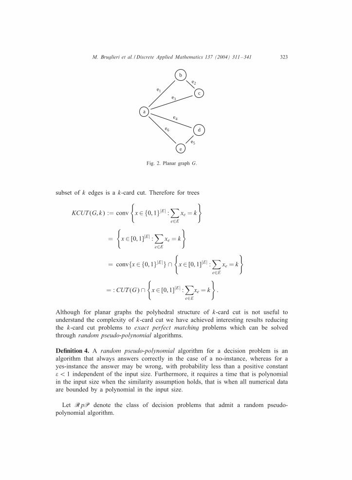
and so we also would have a compact description for the k-card cut polytope. Butunfortunately the opposite inclusion does not hold in (5) as the example below shows.For the graph G drawn in Fig. 2, KCUT (G; 3)=∅ because this graph has only cuts withcardinality 2 or 4. But CUT (G)∩{x∈ [0; 1]|E| :
∑e∈E xe=k} �= ∅ because, for example,
x=(1; 12 ;12 ;
12 ; 0;
12 ) belongs to this set. Indeed, x∈CUT (G) because x= 1
2x′+ 1
2x′′ where
x′=(1; 0; 1; 1; 0; 1) and x′′=(1; 1; 0; 0; 0; 0) are incidence vectors of cuts of G. Moreover,∑e∈E xe = 3: Examples of grid graphs and triangulations for which the equality does
not hold can be easily constructed, too. Are there other graphs for which the twopolyhedra coincide? The answer is yes: trees. Due to the proof of Proposition 8 any
M. Bruglieri et al. / Discrete Applied Mathematics 137 (2004) 311–341 323
b
c
d
e
a
e1
e3
e2
e4
e6
e5
Fig. 2. Planar graph G.
subset of k edges is a k-card cut. Therefore for trees
KCUT (G; k) := conv
{x∈ {0; 1}|E| :
∑e∈E
xe = k
}
=
{x∈ [0; 1]|E| :
∑e∈E
xe = k
}
= conv{x∈ {0; 1}|E|} ∩{x∈ [0; 1]|E| :
∑e∈E
xe = k
}
= :CUT (G) ∩{x∈ [0; 1]|E| :
∑e∈Exe = k
}:
Although for planar graphs the polyhedral structure of k-card cut is not useful tounderstand the complexity of k-card cut we have achieved interesting results reducingthe k-card cut problems to exact perfect matching problems which can be solvedthrough random pseudo-polynomial algorithms.
De�nition 4. A random pseudo-polynomial algorithm for a decision problem is analgorithm that always answers correctly in the case of a no-instance, whereas for ayes-instance the answer may be wrong, with probability less than a positive constant/¡ 1 independent of the input size. Furthermore, it requires a time that is polynomialin the input size when the similarity assumption holds, that is when all numerical dataare bounded by a polynomial in the input size.
Let RpP denote the class of decision problems that admit a random pseudo-polynomial algorithm.
324 M. Bruglieri et al. / Discrete Applied Mathematics 137 (2004) 311–341
De�nition 5. Given an undirected edge-weighted graph G = (V; E) and an integer W ,an exact perfect matching with weight W is a subset of the edge set E which coversall vertices in V once and only once, and has the sum of the weights equal to W .
In the following analysis we will also need the de3nition of a Pfa*an. Given askew-symmetric matrix M of even order the Pfa?an of M , pf(M), is de3ned as
pf(M) :=√det(M);
where det(M) denotes the determinant of M . Given a graph G = (V; E) with vertexset V = {1; : : : ; 2n}, edge set E, |E| = m and an edge-weight function w :E → N, letus consider the 2n× 2n skew-symmetric matrix C
Ci;l =
ti; lyw(e) if e = {i; l} ∈E; i¡ l;
−ti; lyw(e) if e = {i; l} ∈E; i¿ l;
0 otherwise:
Since the determinant of a skew-symmetric matrix of even order is a perfect squarewe can express pf(C) as a polynomial in the variables y and ti; l; {i; l} ∈E:
pf(C) =KW−1∑j=0
qj(t)yj;
where KW is a strict upper bound for the weight of any perfect matching of G, qj(t) isa polynomial in t and t is the vector that collects the ti; l for all {i; l} ∈E.
Lemma 9. There exists an exact perfect matching of weight j in graph G if and onlyif qj(t) is not identically zero in pf(C).
Proof. It has been proved in [25,23] that qj(t) is the sum of all monomials corre-sponding to exact perfect matchings of weight j.
The nice property of pf(C) described in Lemma 9 cannot directly be exploitedbecause it would be a task of exponential complexity to obtain explicitly the monomialsof pf(C), since in general the number of perfect matchings in a graph is exponentiallylarge. However, for 3xed t= Kt pf(C(Kt)) can be evaluated in polynomial time applyingEdmond’s algorithm for computing the determinant of C(Kt) where C(Kt) is seen asa matrix with elements in Z[y], the integrality domain of polynomials in variable y(see [11,16]). So we can understand the shape of pf(C(t)) from pf(C(Kt)) thanks toLemma 1 of [30], which we state below.
Lemma 10. Let q(t1; : : : ; tm) be a polynomial of degree n in m variables and (Kt1; : : : ; Ktm)be chosen randomly in {1; : : : ; N}m. If q is not identically 0, then
Pr{q(Kt1; : : : ; Ktm) = 0}6 nN:

M. Bruglieri et al. / Discrete Applied Mathematics 137 (2004) 311–341 325
v3 v4
v5
v1v2
Fig. 3. The planar graph G and its dual G∗.
Using Lemma 9 and Lemma 10 the image of the perfect matching problem, i.e.the weight of all perfect matchings, can be computed through the following randompseudo-polynomial algorithm proposed in [7].
Algorithm 1. Match(G;w; /)
1. Choose randomly Kt in {1; : : : ; N}m with N = �n=/ ;2. Compute pf(C) for t = Kt;3. For j = 1; : : : ; KW
If qj(Kt) = 0 then no matching having weight j exists;If qj(Kt) �= 0 then a matching having weight j exists;
EndFor.
We notice that when the edge-weight function w achieves only 0− 1 values the Algo-rithm 1 becomes random polynomial (RP) since KW = m=2.Now we have all elements for proving the following result.
Proposition 11. When G = (V; E) is a planar graph the k-card cut is in RP if theedge-weights are uniform and is in RpP if the edge-weights are not uniform.
Let us consider the unweighted case 3rst. Since the graph G is planar it has anassociated geometric dual graph G∗ (see Fig. 3). As a consequence of Theorems 4and 5 of [26] every k-card cut of graph G corresponds to a Eulerian subgraph of G∗
with k edges. Let G be the planar graph with edge weights 0 and 1 obtained in thefollowing way: We replace each vertex v∗i of G∗ with a cycle having length equal to
326 M. Bruglieri et al. / Discrete Applied Mathematics 137 (2004) 311–341
1
1 1
1
1 1
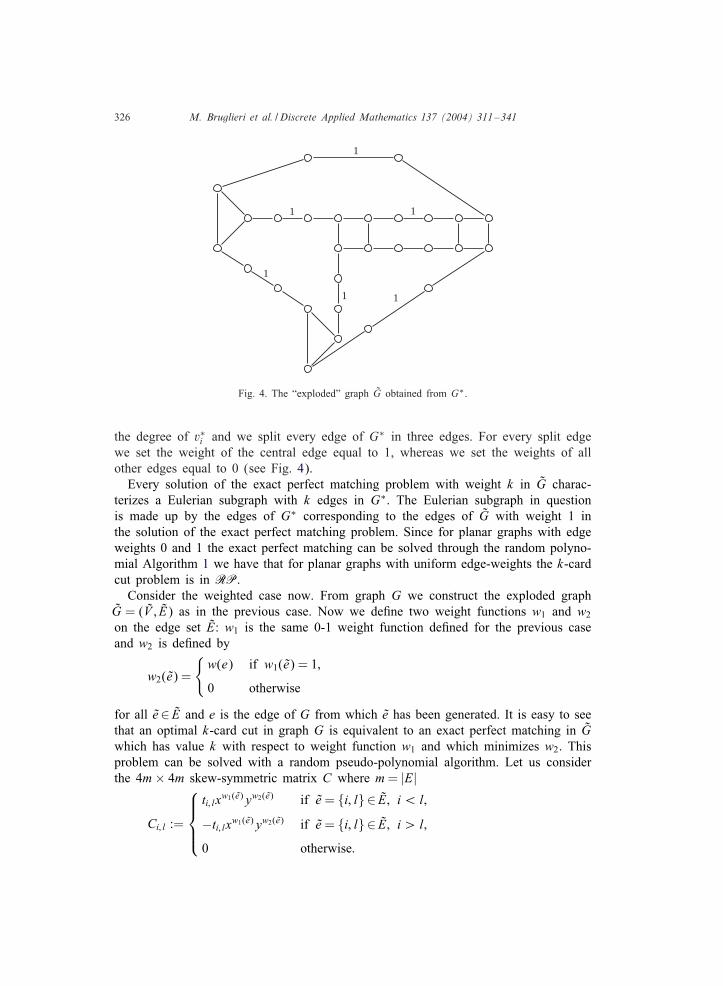
Fig. 4. The “exploded” graph G obtained from G∗.
the degree of v∗i and we split every edge of G∗ in three edges. For every split edgewe set the weight of the central edge equal to 1, whereas we set the weights of allother edges equal to 0 (see Fig. 4).Every solution of the exact perfect matching problem with weight k in G charac-
terizes a Eulerian subgraph with k edges in G∗. The Eulerian subgraph in questionis made up by the edges of G∗ corresponding to the edges of G with weight 1 inthe solution of the exact perfect matching problem. Since for planar graphs with edgeweights 0 and 1 the exact perfect matching can be solved through the random polyno-mial Algorithm 1 we have that for planar graphs with uniform edge-weights the k-cardcut problem is in RP.Consider the weighted case now. From graph G we construct the exploded graph
G = (V ; E) as in the previous case. Now we de3ne two weight functions w1 and w2
on the edge set E: w1 is the same 0-1 weight function de3ned for the previous caseand w2 is de3ned by
w2(e) =
{w(e) if w1(e) = 1;
0 otherwise
for all e∈ E and e is the edge of G from which e has been generated. It is easy to seethat an optimal k-card cut in graph G is equivalent to an exact perfect matching in Gwhich has value k with respect to weight function w1 and which minimizes w2. Thisproblem can be solved with a random pseudo-polynomial algorithm. Let us considerthe 4m× 4m skew-symmetric matrix C where m= |E|
Ci;l :=
ti; lxw1(e)yw2(e) if e = {i; l} ∈ E; i¡ l;
−ti; lxw1(e)yw2(e) if e = {i; l} ∈ E; i¿ l;
0 otherwise:
M. Bruglieri et al. / Discrete Applied Mathematics 137 (2004) 311–341 327
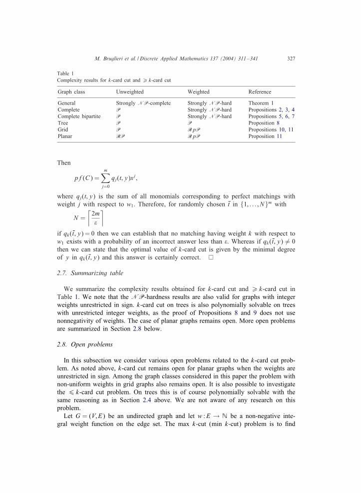
Table 1Complexity results for k-card cut and ¿ k-card cut
Graph class Unweighted Weighted Reference
General Strongly NP-complete Strongly NP-hard Theorem 1Complete P Strongly NP-hard Propositions 2, 3, 4Complete bipartite P Strongly NP-hard Propositions 5, 6, 7Tree P P Proposition 8Grid P RpP Propositions 10, 11Planar RP RpP Proposition 11
Then
pf(C) =m∑j=0
qj(t; y)xj;
where qj(t; y) is the sum of all monomials corresponding to perfect matchings withweight j with respect to w1. Therefore, for randomly chosen Kt in {1; : : : ; N}m with
N =⌈2m/
⌉if qk(Kt; y) = 0 then we can establish that no matching having weight k with respect tow1 exists with a probability of an incorrect answer less than /. Whereas if qk(Kt; y) �= 0then we can state that the optimal value of k-card cut is given by the minimal degreeof y in qk(Kt; y) and this answer is certainly correct.
2.7. Summarizing table
We summarize the complexity results obtained for k-card cut and ¿ k-card cut inTable 1. We note that the NP-hardness results are also valid for graphs with integerweights unrestricted in sign. k-card cut on trees is also polynomially solvable on treeswith unrestricted integer weights, as the proof of Propositions 8 and 9 does not usenonnegativity of weights. The case of planar graphs remains open. More open problemsare summarized in Section 2.8 below.
2.8. Open problems
In this subsection we consider various open problems related to the k-card cut prob-lem. As noted above, k-card cut remains open for planar graphs when the weights areunrestricted in sign. Among the graph classes considered in this paper the problem withnon-uniform weights in grid graphs also remains open. It is also possible to investigatethe 6 k-card cut problem. On trees this is of course polynomially solvable with thesame reasoning as in Section 2.4 above. We are not aware of any research on thisproblem.Let G = (V; E) be an undirected graph and let w :E → N be a non-negative inte-
gral weight function on the edge set. The max k-cut (min k-cut) problem is to 3nd
328 M. Bruglieri et al. / Discrete Applied Mathematics 137 (2004) 311–341
a partition of the vertex set V into k disjoint subsets V = (V1; V2; : : : ; Vk) such thatthe sum of the weights of the crossing edges
∑16r¡s6k
∑i∈Vr ;j∈Vs w({vi; vj}) is max-
imized (minimized). Both the max version and the min version of this problem areNP-hard. For the max k-cut [15] develop an approximation algorithm with a factor1=(1 − 1=k + 2k−2 ln k) via a semide3nite programming relaxation that generalizes theapproach proposed in [20] for the max cut problem. For the min k-cut problem [29]present an approximation algorithm with a factor 2−2=k. A generalization of this graphpartitioning problem is the max (min) k-cut with given size of the parts, that is a max(min) k-cut problem where also the cardinality of each subset Vr of the partition isconstrained to be equal to a 3xed value tr for r = 1; : : : ; k. [1] present a 1=2 approx-imation for the maximization version of this problem. For the minimization versionno constant-factor algorithm is known for general graphs; however, when the edgeweights satisfy the triangle inequality and k is 3xed, [21] present a polynomial-time3-approximation algorithm.Another interesting problem is k-card cut on directed graphs. Concerning the compu-
tational complexity we notice that the cases which are NP-hard on undirected graphsremain so also on directed graphs since we can polynomially reduce the undirectedversion of k-card cut to the directed version doubling each edge in two opposite arcshaving the same weight as in the original graph. On the other hand, the proofs thatk-card cut belongs to P for undirected trees and to RpP for undirected planar graphscannot be immediately adapted to the corresponding directed graphs.
3. Heuristic methods
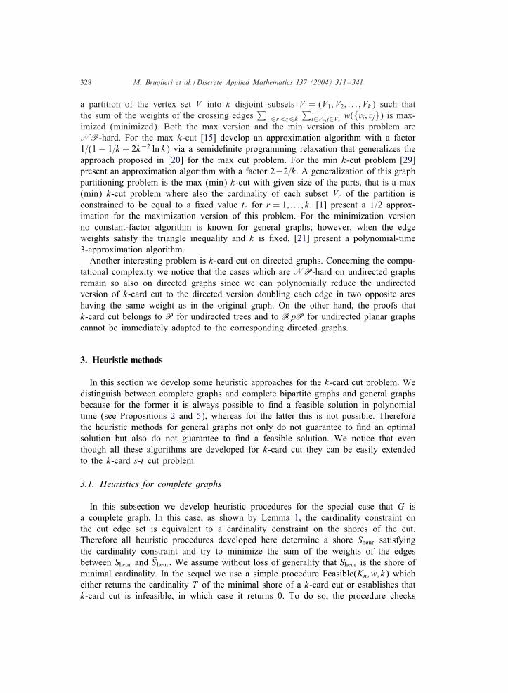
In this section we develop some heuristic approaches for the k-card cut problem. Wedistinguish between complete graphs and complete bipartite graphs and general graphsbecause for the former it is always possible to 3nd a feasible solution in polynomialtime (see Propositions 2 and 5), whereas for the latter this is not possible. Thereforethe heuristic methods for general graphs not only do not guarantee to 3nd an optimalsolution but also do not guarantee to 3nd a feasible solution. We notice that eventhough all these algorithms are developed for k-card cut they can be easily extendedto the k-card s-t cut problem.
3.1. Heuristics for complete graphs
In this subsection we develop heuristic procedures for the special case that G isa complete graph. In this case, as shown by Lemma 1, the cardinality constraint onthe cut edge set is equivalent to a cardinality constraint on the shores of the cut.Therefore all heuristic procedures developed here determine a shore Sheur satisfyingthe cardinality constraint and try to minimize the sum of the weights of the edgesbetween Sheur and KSheur. We assume without loss of generality that Sheur is the shore ofminimal cardinality. In the sequel we use a simple procedure Feasible(Kn; w; k) whicheither returns the cardinality T of the minimal shore of a k-card cut or establishes thatk-card cut is infeasible, in which case it returns 0. To do so, the procedure checks
M. Bruglieri et al. / Discrete Applied Mathematics 137 (2004) 311–341 329
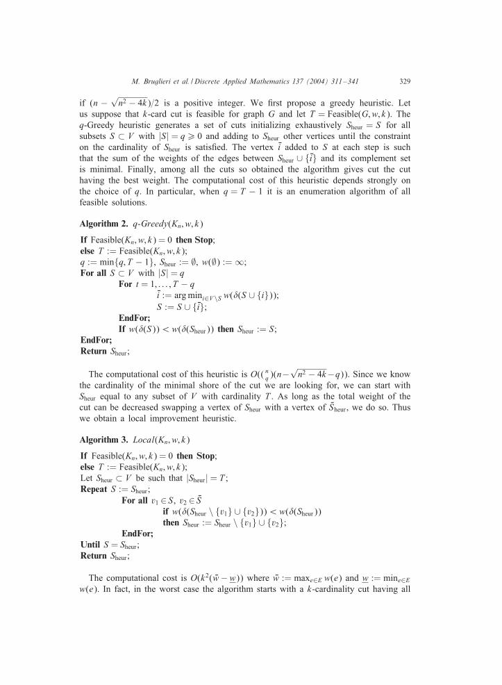
if (n − √n2 − 4k)=2 is a positive integer. We 3rst propose a greedy heuristic. Let
us suppose that k-card cut is feasible for graph G and let T = Feasible(G;w; k). Theq-Greedy heuristic generates a set of cuts initializing exhaustively Sheur = S for allsubsets S ⊂ V with |S| = q¿ 0 and adding to Sheur other vertices until the constrainton the cardinality of Sheur is satis3ed. The vertex Ki added to S at each step is suchthat the sum of the weights of the edges between Sheur ∪ {Ki} and its complement setis minimal. Finally, among all the cuts so obtained the algorithm gives cut the cuthaving the best weight. The computational cost of this heuristic depends strongly onthe choice of q. In particular, when q = T − 1 it is an enumeration algorithm of allfeasible solutions.
Algorithm 2. q-Greedy(Kn; w; k)
If Feasible(Kn; w; k) = 0 then Stop;else T := Feasible(Kn; w; k);q := min{q; T − 1}, Sheur := ∅, w(∅) := ∞;For all S ⊂ V with |S| = q
For t = 1; : : : ; T − qKi := argmini∈V\S w(�(S ∪ {i}));S := S ∪ {Ki};
EndFor;If w(�(S))¡w(�(Sheur)) then Sheur := S;
EndFor;Return Sheur;
The computational cost of this heuristic is O(( nq )(n−√n2 − 4k−q)). Since we know
the cardinality of the minimal shore of the cut we are looking for, we can start withSheur equal to any subset of V with cardinality T . As long as the total weight of thecut can be decreased swapping a vertex of Sheur with a vertex of KSheur, we do so. Thuswe obtain a local improvement heuristic.
Algorithm 3. Local(Kn; w; k)
If Feasible(Kn; w; k) = 0 then Stop;else T := Feasible(Kn; w; k);Let Sheur ⊂ V be such that |Sheur| = T ;Repeat S := Sheur;
For all v1 ∈ S, v2 ∈ KSif w(�(Sheur \ {v1} ∪ {v2}))¡w(�(Sheur))then Sheur := Sheur \ {v1} ∪ {v2};
EndFor;Until S = Sheur;Return Sheur;
The computational cost is O(k2( Kw−w)) where Kw := maxe∈E w(e) and w := mine∈Ew(e). In fact, in the worst case the algorithm starts with a k-cardinality cut having all
330 M. Bruglieri et al. / Discrete Applied Mathematics 137 (2004) 311–341
edge-weights equal to Kw and it stops with a k-cardinality cut having all edge-weightsequal to w and at each step the solution only improves by one unit. Therefore thecomplexity is (k Kw−kw)T (n−T )=k2( Kw−w) since from the de3nition of T , T (n−T )=k.
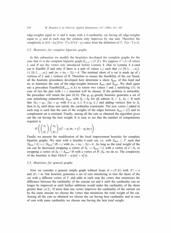
3.2. Heuristics for complete bipartite graphs
In this subsection we modify the heuristics developed for complete graphs for thecase that G is the complete bipartite graph Kn1 ;n2 =(V; E). We suppose V =L∪R whereL and R are the vertex sets introduced before Lemma 4. Due to Lemma 4 k-cardcut is feasible if and only if there is a pair of values i; j such that j∈ {0; 1; : : : ; n2},i∈ {0; 1; : : : ; n1} and jn1 + in2 − 2ij = k. The minimal shore of a cut is made up of ivertices of L and j vertices of R. Therefore to ensure the feasibility of the cut found,all the heuristic procedures developed here determine a shore Sheur of this kind andtry to minimize the sum of the edge-weights between Sheur and KSheur. We shall againuse a procedure Feasible2(Kn1 ;n2 ; w; k) to return two values i and j satisfying (3). Incase of ties the pair with i + j maximal will be chosen. If the problem is infeasible,the procedure will return the pair (0; 0): The q1; q2-greedy heuristic generates a set ofcuts initializing exhaustively Sheur with SL ∪ SR for all subsets SL ⊂ L, SR ⊂ R suchthat |SL| = q1, |SR| = q2 with 06 q16 i, 06 q26 j and adding vertices 3rst to SLthen to SR until these sets satisfy the cardinality constraints. The new vertex Ki added ineach step is such that the sum of the weights of the edges between Sheur ∪ {Ki} and itscomplement set is minimal. Finally, among all the cuts so obtained the algorithm givesout the cut having the best weight. It is easy to see that the number of computationsrequired is
O
((n1
q1
)(n2
q2
)((i − q1)n1 + (j − q2)n2)
):
Finally we present the modi3cation of the local improvement heuristic for completebipartite graphs. We start with a feasible k-card cut, i.e. with Sheur ⊂ V such that|Sheur ∩L|= i, |Sheur ∩R|= j with jn1 + in2 − 2ij= k. As long as the total weight of thecut can be decreased swapping a vertex of SL := Sheur ∩ L with a vertex of L \ SL orswapping a vertex of SR := Sheur ∩R with a vertex of R\SR, we do so. The complexityof the heuristic is then O(k( Kw − w)(n21 + n
22)).
3.3. Heuristics for general graphs
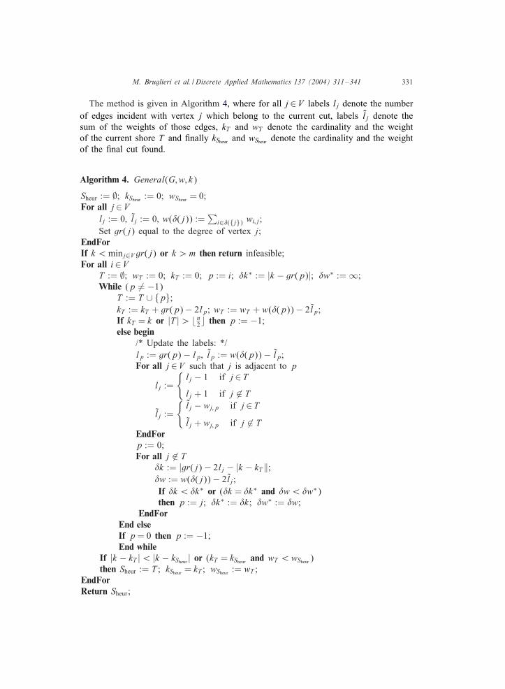
Now we consider a general simple graph without loops G = (V; E) with |V | = nand |E| = m. Our heuristic generates a set of cuts initializing in turn the shore of thecut with a diJerent vertex of V and adds in each step the vertex that minimizes thediJerence between the cardinality of the current cut and k until the cardinality can nolonger be improved or until further additions would make the cardinality of the shoregreater than n=2. If more than one vertex improves the cardinality of the current cutby the same amount we choose the vertex that minimizes the total weight of the cut.Among all the cuts so obtained we choose the cut having best cardinality and in caseof cuts with same cardinality we choose one having the best total weight.
M. Bruglieri et al. / Discrete Applied Mathematics 137 (2004) 311–341 331
The method is given in Algorithm 4, where for all j∈V labels lj denote the numberof edges incident with vertex j which belong to the current cut, labels lj denote thesum of the weights of those edges, kT and wT denote the cardinality and the weightof the current shore T and 3nally kSheur and wSheur denote the cardinality and the weightof the 3nal cut found.
Algorithm 4. General(G;w; k)
Sheur := ∅; kSheur := 0; wSheur = 0;For all j∈V
lj := 0; lj := 0; w(�(j)) :=∑
i∈�({j}) wi;j;Set gr(j) equal to the degree of vertex j;
EndForIf k ¡minj∈V gr(j) or k ¿m then return infeasible;For all i∈V
T := ∅; wT := 0; kT := 0; p := i; �k∗ := |k − gr(p)|; �w∗ := ∞;While (p �= −1)
T := T ∪ {p};kT := kT + gr(p) − 2lp; wT := wT + w(�(p)) − 2lp;If kT = k or |T |¿ n2 then p := −1;else begin
/* Update the labels: */lp := gr(p) − lp; lp := w(�(p)) − lp;For all j∈V such that j is adjacent to p
lj :=
{lj − 1 if j∈Tlj + 1 if j �∈ T
lj :=
{lj − wj;p if j∈Tlj + wj;p if j �∈ T
EndForp := 0;For all j �∈ T
�k := |gr(j) − 2lj − |k − kT‖;�w := w(�(j)) − 2lj;If �k ¡�k∗ or (�k = �k∗ and �w¡�w∗)then p := j; �k∗ := �k; �w∗ := �w;
EndForEnd elseIf p= 0 then p := −1;End while
If |k − kT |¡ |k − kSheur | or (kT = kSheur and wT ¡wSheur )then Sheur := T ; kSheur = kT ; wSheur := wT ;
EndForReturn Sheur;
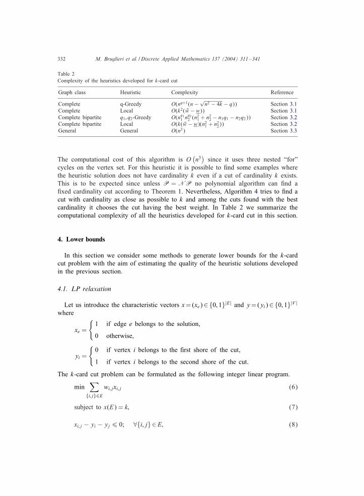
332 M. Bruglieri et al. / Discrete Applied Mathematics 137 (2004) 311–341
Table 2Complexity of the heuristics developed for k-card cut
Graph class Heuristic Complexity Reference
Complete q-Greedy O(nq+1(n− √n2 − 4k − q)) Section 3.1
Complete Local O(k2( Kw − w)) Section 3.1Complete bipartite q1; q2-Greedy O(nq11 n
q22 (n21 + n
22 − n1q1 − n2q2)) Section 3.2
Complete bipartite Local O(k( Kw − w)(n21 + n22)) Section 3.2
General General O(n3) Section 3.3
The computational cost of this algorithm is O(n3)since it uses three nested “for”
cycles on the vertex set. For this heuristic it is possible to 3nd some examples wherethe heuristic solution does not have cardinality k even if a cut of cardinality k exists.This is to be expected since unless P =NP no polynomial algorithm can 3nd a3xed cardinality cut according to Theorem 1. Nevertheless, Algorithm 4 tries to 3nd acut with cardinality as close as possible to k and among the cuts found with the bestcardinality it chooses the cut having the best weight. In Table 2 we summarize thecomputational complexity of all the heuristics developed for k-card cut in this section.
4. Lower bounds
In this section we consider some methods to generate lower bounds for the k-cardcut problem with the aim of estimating the quality of the heuristic solutions developedin the previous section.
4.1. LP relaxation
Let us introduce the characteristic vectors x=(xe)∈ {0; 1}|E| and y=(yi)∈ {0; 1}|V |
where
xe =
{1 if edge e belongs to the solution;
0 otherwise;
yi =
{0 if vertex i belongs to the 3rst shore of the cut;
1 if vertex i belongs to the second shore of the cut:
The k-card cut problem can be formulated as the following integer linear program.
min∑
{i; j}∈Ewi; jxi; j (6)
subject to x(E) = k; (7)
xi; j − yi − yj6 0; ∀{i; j} ∈E; (8)
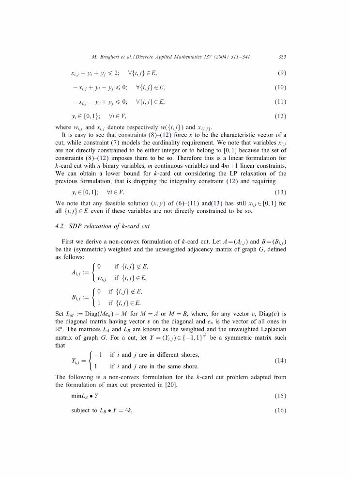
M. Bruglieri et al. / Discrete Applied Mathematics 137 (2004) 311–341 333
xi; j + yi + yj6 2; ∀{i; j} ∈E; (9)
− xi; j + yi − yj6 0; ∀{i; j} ∈E; (10)
− xi; j − yi + yj6 0; ∀{i; j} ∈E; (11)
yi ∈ {0; 1}; ∀i∈V; (12)
where wi;j and xi; j denote respectively w({i; j}) and x{i; j}.It is easy to see that constraints (8)–(12) force x to be the characteristic vector of a
cut, while constraint (7) models the cardinality requirement. We note that variables xi; jare not directly constrained to be either integer or to belong to [0; 1] because the set ofconstraints (8)–(12) imposes them to be so. Therefore this is a linear formulation fork-card cut with n binary variables, m continuous variables and 4m+1 linear constraints.We can obtain a lower bound for k-card cut considering the LP relaxation of theprevious formulation, that is dropping the integrality constraint (12) and requiring
yi ∈ [0; 1]; ∀i∈V: (13)
We note that any feasible solution (x; y) of (6)–(11) and(13) has still xi; j ∈ [0; 1] forall {i; j} ∈E even if these variables are not directly constrained to be so.
4.2. SDP relaxation of k-card cut
First we derive a non-convex formulation of k-card cut. Let A=(Ai;j) and B=(Bi;j)be the (symmetric) weighted and the unweighted adjacency matrix of graph G, de3nedas follows:
Ai;j :=
{0 if {i; j} �∈ E;wi; j if {i; j} ∈E;
Bi; j :=
{0 if {i; j} �∈ E;1 if {i; j} ∈E:
Set LM := Diag(Men) −M for M = A or M = B, where, for any vector v, Diag(v) isthe diagonal matrix having vector v on the diagonal and en is the vector of all ones inRn. The matrices LA and LB are known as the weighted and the unweighted Laplacianmatrix of graph G. For a cut, let Y = (Yi; j)∈ {−1; 1}n2 be a symmetric matrix suchthat
Yi; j =
{−1 if i and j are in diJerent shores;
1 if i and j are in the same shore:(14)
The following is a non-convex formulation for the k-card cut problem adapted fromthe formulation of max cut presented in [20].
minLA • Y (15)
subject to LB • Y = 4k; (16)
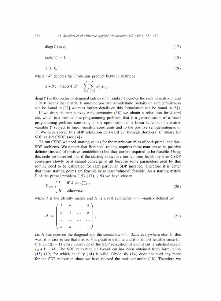
334 M. Bruglieri et al. / Discrete Applied Mathematics 137 (2004) 311–341
diag(Y ) = en; (17)
rank(Y ) = 1; (18)
Y ¡ 0; (19)
where “•” denotes the Frobenius product between matrices
A • B := trace(ATB) =n∑i=1
n∑j=1
Ai;jBi; j ;
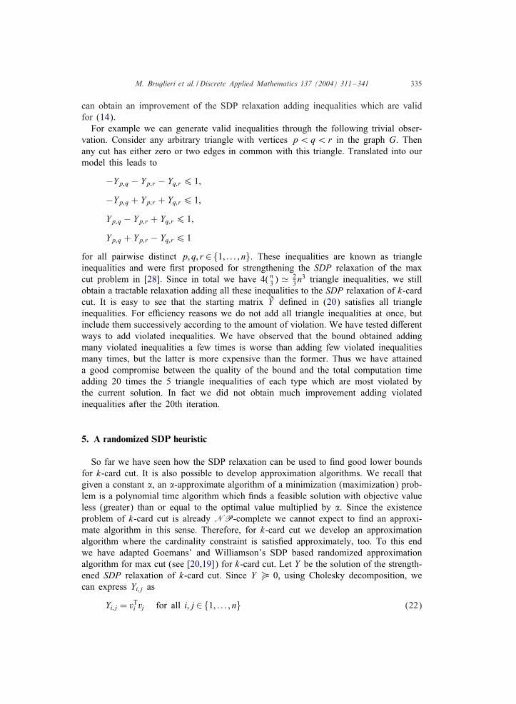
diag(Y ) is the vector of diagonal entries of Y , rank(Y ) denotes the rank of matrix Y andY ¡ 0 means that matrix Y must be positive semide3nite (details on semide3nitenesscan be found in [32] whereas further details on this formulation can be found in [5]).If we drop the non-convex rank constraint (18) we obtain a relaxation for k-card
cut, which is a semide3nite programming problem, that is a generalization of a linearprogramming problem consisting in the optimization of a linear function of a matrixvariable Y subject to linear equality constraints and to the positive semide3niteness ofY . We have solved this SDP relaxation of k-card cut through Borchers’ C library forSDP called CSDP (see [4]).To run CSDP we need starting values for the matrix-variables of both primal and dual
SDP problems. We remark that Borchers’ routine requires these matrices to be positivede3nite (instead of positive semide3nite) but they are not required to be feasible. Usingthis code we observed that if the starting values are too far from feasibility then CSDPconverges slowly or it cannot converge at all because some parameters used by thisroutine need to be calibrated for each particular SDP instance. Therefore it is betterthat those starting points are feasible or at least “almost” feasible. As a starting matrixY of the primal problem (15)–(17), (19) we have chosen
Y :=
{I if k¿ mn
2(n−1) ;
H otherwise;(20)
where I is the identity matrix and H is a real symmetric n× n-matrix de3ned by
H :=
1 a : : : a
a 1 : : : a
: : : : : : : : : : : :
a a : : : 1
; (21)
i.e. H has ones on the diagonal and the constant a=1− 2k=m everywhere else. In thisway, it is easy to see that matrix Y is positive de3nite and it is almost feasible since fork¿mn=2(n−1) every constraint of the SDP relaxation of k-card cut is satis3ed exceptLB • Y = 4k. The SDP relaxation of k-card cut has been obtained from formulation(15)–(19) for which equality (14) is valid. Obviously (14) does not hold any morefor the SDP relaxation since we have relaxed the rank constraint (18). Therefore we
M. Bruglieri et al. / Discrete Applied Mathematics 137 (2004) 311–341 335
can obtain an improvement of the SDP relaxation adding inequalities which are validfor (14).For example we can generate valid inequalities through the following trivial obser-
vation. Consider any arbitrary triangle with vertices p¡q¡r in the graph G. Thenany cut has either zero or two edges in common with this triangle. Translated into ourmodel this leads to
−Yp;q − Yp;r − Yq;r6 1;
−Yp;q + Yp;r + Yq;r6 1;
Yp;q − Yp;r + Yq;r6 1;
Yp;q + Yp;r − Yq;r6 1
for all pairwise distinct p; q; r ∈ {1; : : : ; n}. These inequalities are known as triangleinequalities and were 3rst proposed for strengthening the SDP relaxation of the maxcut problem in [28]. Since in total we have 4( n3 ) � 2
3n3 triangle inequalities, we still
obtain a tractable relaxation adding all these inequalities to the SDP relaxation of k-cardcut. It is easy to see that the starting matrix Y de3ned in (20) satis3es all triangleinequalities. For e*ciency reasons we do not add all triangle inequalities at once, butinclude them successively according to the amount of violation. We have tested diJerentways to add violated inequalities. We have observed that the bound obtained addingmany violated inequalities a few times is worse than adding few violated inequalitiesmany times, but the latter is more expensive than the former. Thus we have attaineda good compromise between the quality of the bound and the total computation timeadding 20 times the 5 triangle inequalities of each type which are most violated bythe current solution. In fact we did not obtain much improvement adding violatedinequalities after the 20th iteration.
5. A randomized SDP heuristic
So far we have seen how the SDP relaxation can be used to 3nd good lower boundsfor k-card cut. It is also possible to develop approximation algorithms. We recall thatgiven a constant 9, an 9-approximate algorithm of a minimization (maximization) prob-lem is a polynomial time algorithm which 3nds a feasible solution with objective valueless (greater) than or equal to the optimal value multiplied by 9. Since the existenceproblem of k-card cut is already NP-complete we cannot expect to 3nd an approxi-mate algorithm in this sense. Therefore, for k-card cut we develop an approximationalgorithm where the cardinality constraint is satis3ed approximately, too. To this endwe have adapted Goemans’ and Williamson’s SDP based randomized approximationalgorithm for max cut (see [20,19]) for k-card cut. Let Y be the solution of the strength-ened SDP relaxation of k-card cut. Since Y ¡ 0, using Cholesky decomposition, wecan express Yi; j as
Yi; j = vTi vj for all i; j∈ {1; : : : ; n} (22)
336 M. Bruglieri et al. / Discrete Applied Mathematics 137 (2004) 311–341
for some vectors vi ∈Rn with ‖vi‖=1 for i=1; : : : ; n (see [24]). Let r be a randomlyselected vector on the unit sphere {x∈Rn : ‖x‖ = 1}. The hyperplane orthogonal to rseparates the vectors vi into two sets
V1 = {i∈V : vTi r6 0} and V2 = KV 1: (23)
(V1; V2) is chosen as the random cut. This is referred to as the random hyperplanetechnique. We want to show that this random cut enjoys an approximation propertysimilar to the one described for max cut in [4,20]. The probability that a given edge{i; j} is in the random cut is equal to the probability that the random hyperplaneseparates vi and vj. This is equal to the ratio of the angle between vectors vi and vjand :. Thus the expected value of the cardinality of the random cut is
E[card(cut)] =∑
{i; j}∈E
arccos(vTi vj):
: (24)
Since
0:878561 − x2
6arccos(x)
:6
1 − x2
1:13822
for −16 x6 1 we have that with (22)
0:87856∑
{i; j}∈E
1 − Yi; j2
6E[card(cut)]6 1:13822∑
{i; j}∈E
1 − Yi; j2
: (25)
Since Y is a solution of the SDP relaxation of k-card cut it satis3es the constraintLB • Y = 4k which is equivalent to∑
{i; j}∈E
1 − Yi; j2
= k
(see [5] for further details). Thus (25) can be rewritten as
0:87856k6E[card(cut)]6 1:13822k: (26)
Hence formula (26) ensures that the expected value on the cardinality of the randomcut belongs to a small neighbourhood of k. With regard to the expected value of theweight of the cut we 3nd through similar arguments
E[w(cut)]6 1:13822∑
{i; j}∈Ewi; j
1 − Yi; j2
: (27)
The sum in (27) is equal to the objective function of the strengthened SDP relaxationof k-card cut. Since Y is a solution of this relaxation, the sum in (27) is less than theoptimal value w∗ of k-card cut. Hence we obtain
E[w(cut)]6 1:13822w∗: (28)
The approximation properties (26) and (28) we have shown hold for the expected valueof the cardinality and weight of the random cut whereas no approximation properties
M. Bruglieri et al. / Discrete Applied Mathematics 137 (2004) 311–341 337
are obtained for a single random cut. Therefore for exploiting these approximationproperties we have considered several uniform random vectors. For each of them wehave generated a random cut through the random hyperplane technique. Among all therandom cuts so obtained we have chosen the one with cardinality as close as possibleto k and in case of cuts with same cardinality we have chosen the one having the besttotal weight.
6. Numerical results
6.1. Description of the instances for k-card cut
Since the k-card cut problem has never been considered in the literature no validationinstances are publicly available. Therefore we have generated instances of the k-cardcut problem for all graph classes examined in this work according to Table 3. Generalgraphs have been generated considering vertices with uniformly distributed randomdegree in order to have an edge density of 50%. Planar graphs have been generatedconsidering as vertices uniformly distributed random points in a square and linking pairsof them by an edge only if the edge does not cross any edges previously generatedand until an edge density equal or less than 50% is achieved. All graphs have randominteger weights on the edges uniformly distributed between 1 and 100. For completeand complete bipartite graphs we have generated instances of k-card cut for all feasiblevalues of k, whereas for planar graphs and general graphs we have considered as valuesof k the cardinalities of the cuts generated by random partitions of the vertex set.All these instances are publicly available at the web site http://www.elet.polimi.it/
upload/bruglier/kcut.html#instances.
6.2. Numerical results
All the heuristics presented were implemented in C and run on a AMD K7 1 GHzcomputer with 1:2 GB RAM under the Linux 2.2.14 operating system. For the smaller
Table 3Instances generated for k-card cut
Graph class No. of Vertices Edges Values No. ofgraphs of k instances
Complete 20 25 300 12 240Complete 10 100 4950 50 500Complete bipartite 10 20 + 10 200 55 550Complete bipartite 12 40 + 30 1200 273 3276Planar graphs 10 30 60–70 30 300Planar graphs 10 150 370–389 30 300General graphs 10 30 210–226 30 300General graphs 10 150 5530–5665 30 300
338 M. Bruglieri et al. / Discrete Applied Mathematics 137 (2004) 311–341
0 5 10 15 20 25 30 35 40 45 500
1
2
3
4
5
6
7
8
9
10
Shore cardinality
Dev
iatio
n%
GreedyLocalSdp
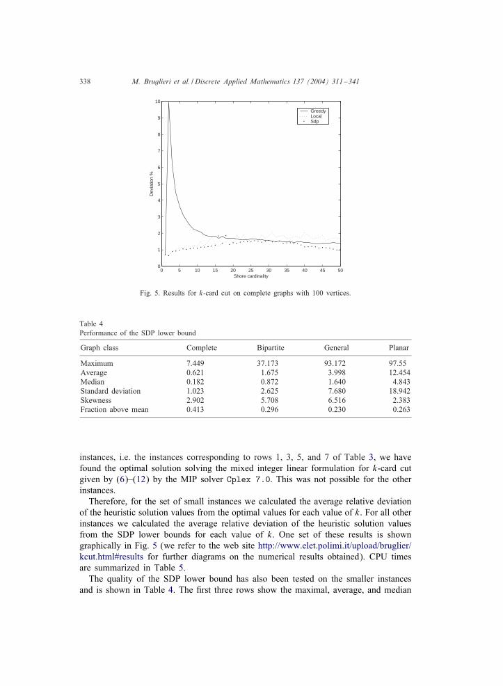
Fig. 5. Results for k-card cut on complete graphs with 100 vertices.
Table 4Performance of the SDP lower bound
Graph class Complete Bipartite General Planar
Maximum 7.449 37.173 93.172 97.55Average 0.621 1.675 3.998 12.454Median 0.182 0.872 1.640 4.843Standard deviation 1.023 2.625 7.680 18.942Skewness 2.902 5.708 6.516 2.383Fraction above mean 0.413 0.296 0.230 0.263
instances, i.e. the instances corresponding to rows 1, 3, 5, and 7 of Table 3, we havefound the optimal solution solving the mixed integer linear formulation for k-card cutgiven by (6)–(12) by the MIP solver Cplex 7.0. This was not possible for the otherinstances.Therefore, for the set of small instances we calculated the average relative deviation
of the heuristic solution values from the optimal values for each value of k. For all otherinstances we calculated the average relative deviation of the heuristic solution valuesfrom the SDP lower bounds for each value of k. One set of these results is showngraphically in Fig. 5 (we refer to the web site http://www.elet.polimi.it/upload/bruglier/kcut.html#results for further diagrams on the numerical results obtained). CPU timesare summarized in Table 5.The quality of the SDP lower bound has also been tested on the smaller instances
and is shown in Table 4. The 3rst three rows show the maximal, average, and median

M. Bruglieri et al. / Discrete Applied Mathematics 137 (2004) 311–341 339
Table 5CPU-time (in s) for the heuristics and for the exact formulation
Graph class Greedy Local General SDP Exact
Complete, 25 0.01–0.25 0.01–0.15 — 18–70 2–99Complete, 100 0.02–937 0.02–433 — 537–923 —Bipartite, 20 + 10 0.01–0.62 0.01–0.1 — 0.46–116 0.83–445Bipartite, 40 + 30 0.01–35 0.04–14 — 2.17–449 —Planar, 30 — — 0.01–0.04 0.76–91 0.12–0.51Planar, 150 — — 0.31–5.18 145–2055 —General, 30 — — 0.01–0.06 41–94 1–79General, 150 — — 5–144 1275–1956 —
deviation from optimality in %, the others show standard deviation, skewness, and thefraction of instances with deviation above average.These numbers indicate that the SDP lower bound works best for complete graphs,
followed by complete bipartite graphs, and is not as good for general and planar graphs.In all classes there is a relatively small number of instances with large deviationswhereas most instances have below average deviations. We notice that the quality ofthe SDP lower bound improves for the bigger instances.Looking at the results we can make some observations. Although there is no dom-
inating relation between the heuristics the SDP and local search heuristics seem tobe more robust than the Greedy heuristic for complete and complete bipartite graphs.Moreover the SDP heuristic reveals to be the most robust heuristic for all other graphclasses. However, in several instances of k-card cut, especially for general and planargraphs the SDP heuristic 3nds a cut with cardinality close to k but not exactly k asrequired. We note that the infeasible solutions found do not appear in the graphics. Ingeneral the results of the SDP heuristic for big instances seem to be better than theresults for small instances. The behaviour of the deviations seem not to depend on thevalue of k: the deviations of instances having big values of k are of the same orderof the deviations of instances with small values of k.In Table 5 we summarize the minimum CPU-times and the maximum CPU-times for
running the heuristics and, when possible, the exact formulation. We can see that therunning time obtained could be improved because the intention of the paper was not ingreatest possible e*ciency of the implemented methods, e.g. no special data structureshave been used. We notice that although the SDP heuristic is the most expensive(for small instances even more expensive than the exact formulation!), however theincrease in CPU time is much less for it than for the other heuristics when the size ofthe instances increases.
Acknowledgements
The authors thank the anonymous referees for their useful suggestions.
340 M. Bruglieri et al. / Discrete Applied Mathematics 137 (2004) 311–341
References
[1] A.A. Ageev, M.I. Sviridenko, Approximation algorithms for maximum coverage and max-cut with givensizes of parts, in: Integer Programming and Combinatorial Optimization, Lecture Notes in ComputerScience, Vol. 1610, Springer, Berlin, 1999, pp. 17–30.
[2] F. Barahona, On some applications of the Chinese postman problem, in: Algorithms and Combinatorics:Paths, Flows, and VLSI-Layout, Springer, Berlin, 1990.
[3] F. Barahona, M. GrYotschel, M. JYunger, G. Reinelt, An application of combinatorial optimization tostatistical physics and circuit layout design, Oper. Res. 36 (3) (1988) 493–513.
[4] B. Borchers, CSDP, a C library for semide3nite programming, Optimization Methods and Software 11(1999) 613–623, http://www.nmt.edu/∼borchers/csdp.html.
[5] M. Bruglieri, K-Cardinality cut problems, Ph.D. Thesis, Dottorato MA.C.R.O., Department ofMathematics ‘F. Enriquez’, University of Milan, 2000. Available at www.elet.polimi.it/upload/bruglier/kcut/PhD-thesis.zip.
[6] R.G. Busacker, T.L. Saaty, Finite Graphs and Networks: An Introduction with Applications,McGraw-Hill, New York, 1965.
[7] P.M. Camerini, G. Galbiati, F. Ma*oli, The image of weighted combinatorial problems, Ann. Oper.Res. 33 (1991) 181–197.
[8] T.J. Chang, N. Meade, J.E. Beasley, Y.M. Sharaiha, Heuristics for cardinality constrained portfoliooptimisation, Comput. Operat. Res. 27 (2000) 1271–1302.
[9] M. Dell’Amico, F. Ma*oli, S. Martello, Annotated Bibliographies in Combinatorial Optimization, Wiley,Chichester, 1997.
[10] M. Dell’Amico, S. Martello, The k-cardinality assignment problem, Discrete Appl. Math. 76 (1997)103–121.
[11] J. Edmonds, Systems of distinct representatives and linear algebra, J. Res. Natl. Bur. Standards 71B(1967) 241–245.
[12] M. Ehrgott, J. Freitag, H.W. Hamacher, F. Ma*oli, Heuristics for the k-cardinality tree and subgraphproblem, Asia Paci3c J. Oper. Res. 14 (1) (1997) 87–114.
[13] M. Ehrgott, H.W. Hamacher, F. Ma*oli, Fixed cardinality combinatorial optimization problems—asurvey, Report in Wirtschaftsmathematik 56 Fachbereich Mathematik, UniversitYat Kaiserslautern, 1999.
[14] L.R. Foulds, H.W. Hamacher, J.M. Wilson, Integer programming approaches to facilities layout modelswith forbidden areas, Ann. Oper. Res. 81 (1998) 405–417.
[15] A. Frieze, M. Jerrum, Improved approximation algorithms for max k-cut and max bisection,Algorithmica 18 (1997) 67–81.
[16] G. Galbiati, F. Ma*oli, On the computation of Pfa*ans, Discrete Appl. Math. 51 (1994) 269–275.[17] M.R. Garey, D.S. Johnson, Computers and Intractability: A Guide to the Theory of NP-Completeness,
Freeman, San Francisco, 1979.[18] M.R. Garey, D.S. Johnson, L. Stockmeyer, Some simpli3ed NP-complete graph problems, Theoret.
Comput. Sci. 1 (1976) 237–267.[19] M.X. Goemans, Semide3nite programming in combinatorial optimization, Math. Programming 79 (1997)
143–161.[20] M.X. Goemans, D.P. Williamson, Improved approximation algorithms for maximum cut and satis3ability
problems using semide3nite programming, J. ACM 42 (1995) 1115–1145.[21] N. Guttmann-Beck, R. Hassin, Approximation algorithms for minimum k-cut, Algorithmica 27 (2)
(2000) 198–207.[22] D. Karger, Minimum cuts in near-linear time, http://theory.lcs.mit.edu//∼karger.[23] R.M. Karp, E. Upfal, A. Widgerson, Constructing a perfect matching is in Random NC, Combinatorica
6 (1) (1986) 35–48.[24] P. Lancaster, M. Tismenetsky, The Theory of Matrices, Academic Press, Orlando, 1985.[25] L. Lovasz, On determinants, matchings and random algorithms, Fund. Comput. Theory 79 (1979)
565–574.[26] G.I. Orlova, Y.G. Dorfman, Finding the maximum cut in a graph, Eng. Cybernet. 10 (1972) 502–506.[27] M. Padberg, G. Rinaldi, An e*cient algorithm for the minimum capacity cut problem, Math.
Programming 47 (1990) 19–39.
M. Bruglieri et al. / Discrete Applied Mathematics 137 (2004) 311–341 341
[28] S. Poljak, F. Rendl, Nonpolyhedral relaxations of graph-bisection problems, SIAM J. Optim. 5 (1995)467–487.
[29] H. Saran, V. Vazirani, Finding k-cuts within twice the optimal, in: Proceedings of the 32nd AnnualIEEE Symposium on Foundations of Computer Science, IEEE Press, Piscataway NJ, 1991, pp. 743–751.
[30] J.T. Schwartz, Fast probabilistic algorithms for veri3cation of polynomial identities, J. Assoc. Comput.Machinery 27 (1980) 701–717.
[31] M. Stoer, F. Wagner, A simple min-cut algorithm, J. ACM 44 (1997) 585–591.[32] H. Wolkowicz, R. Saigal, L. Vandenberghe, Handbook of Semide3nite Programming: Theory,
Algorithms, and Applications, Kluwer Academic Publishers, Dordrecht, 2000.