HAL Id: halshs-00009118https://halshs.archives-ouvertes.fr/halshs-00009118

Submitted on 24 Mar 2006

HAL is a multi-disciplinary open accessarchive for the deposit and dissemination of sci-entific research documents, whether they are pub-lished or not. The documents may come fromteaching and research institutions in France orabroad, or from public or private research centers.

L’archive ouverte pluridisciplinaire HAL, estdestinée au dépôt et à la diffusion de documentsscientifiques de niveau recherche, publiés ou non,émanant des établissements d’enseignement et derecherche français ou étrangers, des laboratoirespublics ou privés.

Cartographic Modelling with Geographical InformationSystems for Determination of Water Resources

VulnerabilityFrançois Laurent, Wolfram Anker, Didier Graillot

To cite this version:François Laurent, Wolfram Anker, Didier Graillot. Cartographic Modelling with Geographical In-formation Systems for Determination of Water Resources Vulnerability. Journal of American WaterResources Association, Journal of American Water Resources Association, 1998, 34 (1), pp.123-134.<halshs-00009118>

Spatial Modelling with Geographic Information Systems

for Determination of Water Resources Vulnerability

Application to an area in Massif Central (France)1

François Laurent, Wolfram Anker and Didier Graillot2

ABSTRACT: A method for water resources protection based on spatial variability of vulnerability is

proposed. The vulnerability of a water resource is defined as the risk that the resource will become

contaminated if a pollutant is placed on the surface at one point as compared to another. A spatial

modelling method is defined in this paper to estimate a travel time between any point of a catchment and

a resource (river or well). This method is based on spatial analysis tools integrated in Geographical

Information Systems (GIS). The method is illustrated by an application to an area of Massif Central

(France) where three different types of flow appear: surface flow, shallow subsurface flow and

permanent groundwater flow (baseflow). The proposed method gives results similar to classical

methods of estimation of travel time. The contribution of GIS is to improve the mapping of vulnerability

by taking the spatial variability of physical phenomena into account.

(KEY TERMS: Water Resources Protection, GIS, Watershed Management, Pollution Modeling,

Spatial Modeling, Massif Central)

INTRODUCTION

Protection of water resources (rivers or aquifers) against pollution is an important challenge for decision-

makers in water resources. To make the decisions necessary to reduce the impact of potential polluting

1 Paper No. 95152R of the Water Resources Bulletin.

activities, it is necessary to consider the vulnerability of the water resource. The vulnerability of a water

resource to a pollution event can be defined as the risk that the resource will become contaminated if a

pollutant is released at one point of the surface as compared to another point (Maidment, 1993). The

vulnerability depends on the intrinsic ability of the natural medium to transfer a pollutant. The water

resource in this context can be a river, a lake, an aquifer or a well. When the whole aquifer is regarded

as a resource and not simply as a pathway for pollution towards rivers or wells, it is necessary to

identify the watershed which flows into the aquifer by lateral inputs.

The aim of a vulnerability map is to define the areas vulnerable to a priori unknown but dissolved

pollution: pollution type, duration, location, quantity and nature (Albinet and Margat, 1970). A map of

water resource vulnerability could serve to protect the most vulnerable sections (for example by

reconversion of intensive agriculture areas, collection of wastewater, plantation of riparian forest) and to

analyse the impact of a proposed activity which presents a pollution risk.

The map can also be used to locate new wells or new diversions of rivers or lakes. Indeed, it would be

more relevant to choose a site not only on criteria such as discharge or immediate water quality but also

on the potential risk of future pollution (Laurent, 1996).

GIS and water resources

GIS have many applications in water resources management and hydrology. The knowledge of terrain

and land cover features is improved by GIS which are used to analyze topographic slope, channel

length, land use and soil characteristics of a watershed (Maidment, 1993 ; La Berbera et al., 1993). The

topological data structures of GIS allows the hydrologists to increase the degree of definition of spatial

units into the distributed models (Maidment, 1993). Spatial modelling with the GIS is used to extract

2 Respectively Assistant Professor, PhD-student, Professor, Ecole des Mines, Laboratoire Ingénierie de

relevant information such as slope, watershed limits or flowpath (O’Callaghan and Mark, 1984 ; Jenson

and Domingue, 1988 ; Quinn,1991 ; Quinn et al., 1991).

GIS have been used for the determination of vulnerabilty of groundwater. DRASTIC (Depth to water,

net Recharge, Aquifer media, Topography, Impact of vadose zone, hydraulic conductivity of the

aquifer) (Aller et al., 1987) and SEEPAGE (System for Early Evaluation of Pollution Potential of

Agricultural Groundwater Systems) (Richert et al., 1992) are methods based on an overlapping of

numerical map sheets. A weight is assigned to each geographical layer and a score is obtained which

represents the vulnerability. There are some similar approaches using muticriteria analysis in other

countries of the world (for example: Munoz and Langevin, 1991, in Guatemala ; Peverieri et al., 1991,

in Italia). In United States, these models are applied on a regional scale (from 1 : 250,000 to 1 :

2,000,000) (Navulur and Engel, 1996).

The existing methodologies for producing water resource vulnerability maps are based on an

overlapping of criteria and not on an analysis of pollutant motion. These methodologies are used to

evaluate a vulnerability representative of spatial unities but their is no relation between the unities. There

are no explicit physical laws imbedded in the model relationships (Maidment, 1993). These methods

ignore the dynamics of the groundwater flow system (Snyder and Wilkinson, 1992), the results depend

on the weights assigned to each criterion and do not take the flow path into account. GIS are used only

to automatize overlapping but the methodology is similar to the manual approaches (Laurent, 1996).

Contaminant transport in soil is modelled by field scale models as GLEAMS (Ground Loading Effects

of Agricultural Management Systems), NLEAP (Nitrate Leaching and Economic Analysis Package),

MikeShe (Hydrologic European System) (Vested et al., 1992) or RUSTIC (Risk of Unsaturated /

l’Environnement, 158, Cours Fauriel, 42023 Saint-Etienne, France.

Saturated Transport and Transformation of Chemical Concentrations) for nonpoint agricultural pollution.

But, the field scale models require more detailed data like evaporation, hydraulic parameters or

management practices (Navulur and Engel, 1996). These models are used on small watersheds because

the high level of detailed parameters of inputs is to expensive on large areas.

Snyder and Wilkinson (1992) have used groundwater flow models in conjunction with partcle tracking

to evaluate aquifer vulnerability. The method is based on the delineation of recharge areas for a

hydrogeologic unit by tracking particles backward from each cell in the unit to their recharge points. A

minimum travel time is evaluated between each cell and its recharge points. The DRASTIC rating

calculated on each cell is used with the travel time to determine aquifer vulnerability.

The method for vulnerability mapping proposed in this paper is based on the flow path and the travel

time between any point of the watershed and a well or a river. No weighting is used in this method.

Topography and soils are used to determine flow types, flow path and velocities. Saturated areas which

result in quick flow are located and the interactions between surface water and groundwater are taken

into account.

PARAMETERS CONTROLLING WATER RESOURCES VULNERABILITY

The vulnerability criterion considered here is the minimum transfer time between a pollution point and a

water resource (Laurent et al., 1995). As Barrocu and Biallo (1993) have pointed out, pollution danger

decreases when transfer time increases, because if the travel time is long enough, it is possible to

intervene in order to stop the pollutant’s propagation or to look for an alternate resource (see also,

Lallemand-Barrès and Roux, 1989 ; Snyder and Wilkinson, 1992).

Adsorption, mechanical filtration, biodegradation and dilution phenomena are complex and show great

variability in space and time depending on the kind of pollutant. Modelling of these phenomena at a

catchment scale is impossible without an adequate number of measured data of the catchment’s soil

properties and pollutant concentrations. Therefore, the method presented here does not quantify

concentration variations as a result of the pollutant reduction.

Convection (De Marsily, 1986) is the mechanism of particle transport used in the proposed model: a

space represented by a mesh of regular cells. The displacement of a water volume is assumed to be

without mixing with the neighbouring cells. The concentration in a study cell does not change. This

corresponds to a directed current in which flow velocities are given by Darcy’s Law. A convective flow

model is relevant to calculate the minimum travel time: dispersion processes have tendency to delay

transfer times and diffusion is negligible.

The proposed method allows the creation of a vulnerability map for any soluble pollutant without a

priori knowledge of its chemical nature. Therefore, the vulnerability map will be built from transfer times

of the pollutant from a possible point of release to the considered water resource which can be a river, a

lake or a well exploiting an aquifer.

Therefore, we have to determine the flow path and the velocity (Figure 1) : the pollutant, transported in

a solution, follows a particular path at a given velocity which depends both on the type of flow (surface

or subsurface). Furthermore, a distributed approach must take into account the spatial variability of

parameters which determine the type of flow: soil, topography and meteorological conditions.

MODELLING OF THE DIFFERENT FLOW TYPES

Pollution transport can occur in a catchment through different media. These are via overland flow or via

flow through subsurface porous or fissured medium. The proposed model is applicable to overland flow

and subsurface flow in porous media. For subsurface flow in a fissured medium (karst in limestone or

dolomite, basalt, and gap faults in any consolidated rock), more sophisticated models and more

information such as statistical analysis of fissures are required.

Overland flow

The occurrence of overland flow is controlled by soil hydraulic conductivity, topography and weather.

Impermeable soil horizons prevent infiltration of water and induce overland flow (Pilgrim and Cordery,

1992). Overland flow can also occur on permeable saturated areas. The location of the saturated areas

depends strongly on the topography. The bigger the upstream area, the flatter the terrain at a point, the

more saturated it is. Kirkby has proposed a topographic index which represents the propensity of any

point in the catchment to develop saturated conditions (Kirkby, 1975): ln(a/tanβ), where a is the

upstream area of the point and tanβ is its slope.

The hydrologic model (TOPMODEL) is based on this parameter. TOPMODEL allows to estimate the

discharge at the outlet of a watershed and the saturated areas as function of the topography, the

transmissivity and the meteorological conditions (Beven,1986, and Beven et al., 1995).

To evaluate the overland flow areas it is possible to select the values of the topographic index which

correspond to saturated conditions in a gauged watershed which is similar to and near the study area, in

a humid meteorological period. This calibrated value can be reasonably extrapolated to the study area in

order to estimate the sub-areas showing the tendency of saturation.

Flow through a permanent aquifer

The application of the topographic index is based on the assumption that "the hydraulic gradient of the

saturated zone can be approximated by the local surface topographic slope, tanβ" (Beven et al.,

1995). This assumption is not correct in all geological contexts.

In some types of soil such as sandy sediments or gravels (for example, alluvium), a permanent

subsurface aquifer frequently exists. The hydraulic gradient of such alluvial aquifers is often not similar to

the topographic slope. The topographic index is not appropriate in this geological context to estimate the

saturated areas.

Shallow subsurface flow or interflow

Discontinuities in the soil cause large variations in hydraulic conductivity. Vertical flow can be stopped

when it meets a soil layer of less hydraulic conductivity and the resulting interflow generates a temporary

shallow aquifer. This case can be observed in weathered rocks on low permeable substratum

(weathered sand on granite for instance) or illuviated soil (Pilgrim and Cordery, 1992).

This phenomenon is more significant when the hydraulic conductivity and the porosity of the first

decimeters of subsurface soil are increased by biological activity or human activity such as plowing or

vegetation. Brakensiek and Rawls (1988) have observed a rise of effective porosities of 10 to 20%

after plowing. Skaggs and Khaleel (1982) have measured infiltration velocities two times higher in

grassland than in bare crusted soil.

Flow type and transfer velocity

Overland flow

Surface runoff shows complex dynamics: divergence and convergence of flow vary quickly in space and

time and depend on small scale variability of vegetation and topography. Since surface velocities are

tens or hundreds of meters per hour then the travel time may be considered instantaneous for the

purposes of the model. Indeed, a useful time step for the purpose is one day.

Subsurface flow (for example De Marsily, 1986):

In a porous medium, propagation velocity of a pollution front (m.s-1) can be determined by Darcy's Law

which is defined for a porous medium by:

uk i

peff

=*

ω (1)

where k is the hydraulic conductivity of the aquifer (m.s-1), i is the hydraulic gradient (dimensionless) and

ωeff is the effective porosity (dimensionless).

Data availability for analysis

Detailed, spatial information on aquifer properties (such as hydraulic conductivity) are needed to

determine travel times of a pollutant. However, maps of measured conductivities of soil with high spatial

resolution are rarely available and limited in spatial extent. In most cases, very few measurements exist

for an aquifer of interest.

Therefore, in this study information about physical parameters is only given in a qualitative manner, such

as the type of geological formation or the soil type. Maps of these variables can be different in

resolution, semantic precision, geographic continuity and consist of only symbolic values ("sandy clay"

for example). Therefore, inferences on hydraulic conductivity for determining the vulnerability of water

resources have to use this type of qualitative information.

Hydraulic conductivity is determined by soil texture. Several authors have quantified the relationship

between soil texture and hydraulic conductivity (for example: Saxton et al., 1986, Rawls and

Brakensiek 1983, 1985). However, in most cases, granulometric percentages are not quantified in

geological maps. Often, we find qualitative expressions such as clay sand, sandy silt, etc. which imply a

large range of hydraulic conductivity. These qualitative values allow us to infer a range of soil water

properties by applying geological knowledge.

Therefore, for a range of soils described by texture in geological or soil maps, the largest possible

hydraulic conductivity value is considered to yield the most conservative result.

IMPLEMENTATION INTO GIS

GIS are suitable to deal with the spatial variability of parameters and the spatial analysis tools integrated

into GIS can be used for modelling the travel time of a convective flow.

Maidment (1993, 1996) has emphasized that it is possible to do some hydrologic modelling directly

within GIS, so long as temporal variation is not needed. It is possible to route water through networks

and to estimate the travel time using analogies to traffic flow routing in which each arc of the network is

assigned an impedance and flow is accumulated going downstream through the network (Maidment,

1993). The proposed approach is similar but we do not use a vectorial network of arcs. The subsurface

travel time in the porous medium between any point of a watershed slope and a river or a well is

estimated by means of the Darcy’s law in this paper.

Initial cartographic data

Topographic data (contour or Digital Elevation Model) are used to calculate the topographic index.

Geological data and soil data are used to determine impermeable soil areas where the flow occurs on

the surface and to estimate the hydraulic conductivity and effective porosity of the top soil layer

(between 0 and 0.3 meters) and of the bottom soil layer (between 0.3 and 3 meters), respectively Ktop

and ωtop and Kbot and ωbot.

In the aquifer areas, piezometric data are necessary to calculate the hydraulic gradient, the subsurface

flowpath and the thickness of unsaturated zone (difference between topography and piezometry).

As can be seen in the appendix, a model based on the Darcy’s Law is sensitive to the evaluation of the

hydraulic conductivity and of the hydraulic gradient.

Determination of flow type

Obtaining surface runoff areas on impermeable soil

Impermeable outcroping materials are selected from the map Ktop: clay, marl, consolidated rocks

(granite, schist, gneiss, sandstone, conglomerate, etc.) without soil cover.

Obtaining surface runoff areas generated by topographic location

The Kirkby index ln(a/tanβ) is calculated with the GIS at any point by spatial analysis of the Digital

Terrain Model (Moore et al., 1991). In another granitic area of the Massif Central, the Renaison

watershed, TOPMODEL calibration gives saturated areas for topographic index ln(a/tanβ) > 6 in

highly rainy periods. This threshold value is used in the studied area to extract the potential overland

flow subareas.

Obtaining shallow subsurface flow areas

Occurrence of shallow subsurface flow is determined by the hydraulic conductivity of the lower soil

layer (Laurent et al., 1995).

If the hydraulic conductivity is high (Kbot ≥ 10-4 m.s-1), then no shallow subsurface flow will occur

because vertical drainage will be high enough.

If the hydraulic conductivity is moderate or weak (Kbot < 10-4 m.s-1), the amplitude of the discontinuity

of hydraulic conductivity between bottom and top layer must be tested: a discontinuity is judged

significant if it is greater than the uncertainty of estimated permeabilities which is assumed as a factor of

5 (cf. Appendix). Therefore, if Ktop > 5*Kbot a shallow subsurface flow is supposed to occur.

Obtaining areas with flow through permanent aquifer

Where the geological formation is permeable in several meters in depth, we assume that a permanent

aquifer exists and its hydraulic gradient can be different from the topographic slope.

Mapping the velocities

Parameters of lateral transfer velocities are a function of flow type. In surface runoff areas, an

instantaneous transfer is supposed. The hydraulic gradient is supposed equal to the topographic slope

for the shallow subsurface flow and equal to the piezometric gradient for the flow through a permanent

aquifer.

Another map allows the representation of the vertical transfer velocities in the areas of permanent

aquifer.

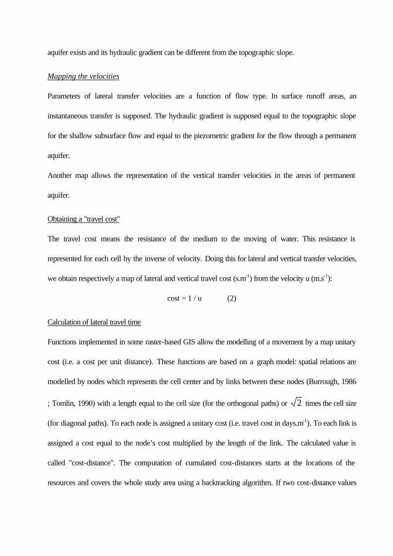
Obtaining a "travel cost"

The travel cost means the resistance of the medium to the moving of water. This resistance is

represented for each cell by the inverse of velocity. Doing this for lateral and vertical transfer velocities,

we obtain respectively a map of lateral and vertical travel cost (s.m-1) from the velocity u (m.s-1):

cost = 1 / u (2)

Calculation of lateral travel time

Functions implemented in some raster-based GIS allow the modelling of a movement by a map unitary

cost (i.e. a cost per unit distance). These functions are based on a graph model: spatial relations are

modelled by nodes which represents the cell center and by links between these nodes (Burrough, 1986

; Tomlin, 1990) with a length equal to the cell size (for the orthogonal paths) or 2 times the cell size

(for diagonal paths). To each node is assigned a unitary cost (i.e. travel cost in days.m-1). To each link is

assigned a cost equal to the node’s cost multiplied by the length of the link. The calculated value is

called "cost-distance". The computation of cumulated cost-distances starts at the locations of the

resources and covers the whole study area using a backtracking algorithm. If two cost-distance values

are obtained in a single link, only the smallest is kept to maintain a conservative estimate.

Typically the flow path is determined by the line of greatest slope and not by a straight line.

For determination of vulnerability, a travel time is calculated for the flow path of each possible pollution

point.

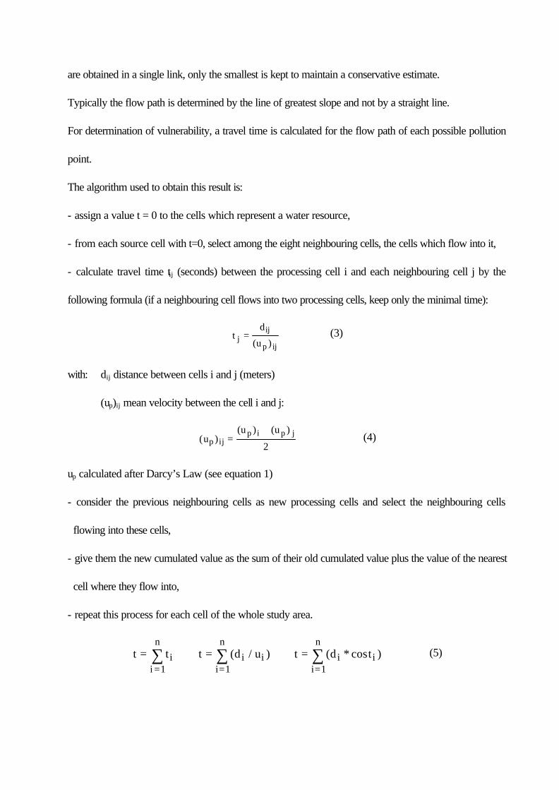
The algorithm used to obtain this result is:

- assign a value t = 0 to the cells which represent a water resource,

- from each source cell with t=0, select among the eight neighbouring cells, the cells which flow into it,

- calculate travel time tij (seconds) between the processing cell i and each neighbouring cell j by the

following formula (if a neighbouring cell flows into two processing cells, keep only the minimal time):

td

ujij

p ij=

( ) (3)

with: dij distance between cells i and j (meters)

(up)ij mean velocity between the cell i and j:

( )( ) ( )

uu u

p ijp i p j

=+

2 (4)

up calculated after Darcy’s Law (see equation 1)

- consider the previous neighbouring cells as new processing cells and select the neighbouring cells

flowing into these cells,

- give them the new cumulated value as the sum of their old cumulated value plus the value of the nearest

cell where they flow into,

- repeat this process for each cell of the whole study area.

t t t d u t d tii

n

i ii

n

i ii

n= ⇒ = ⇒ =

= = =∑ ∑ ∑

1 1 1 ( / ) ( * cos ) (5)

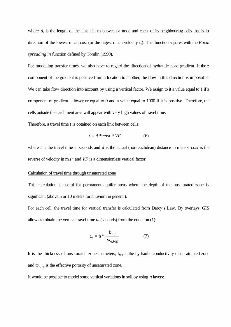
where di is the length of the link i in m between a node and each of its neighbouring cells that is in

direction of the lowest mean cost (or the higest mean velocity ui). This function squares with the Focal

spreading in function defined by Tomlin (1990).

For modelling transfer times, we also have to regard the direction of hydraulic head gradient. If the z

component of the gradient is positive from a location to another, the flow in this direction is impossible.

We can take flow direction into account by using a vertical factor. We assign to it a value equal to 1 if z

component of gradient is lower or equal to 0 and a value equal to 1000 if it is positive. Therefore, the

cells outside the catchment area will appear with very high values of travel time.

Therefore, a travel time t is obtained on each link between cells:

t = d * cost * VF (6)

where t is the travel time in seconds and d is the actual (non-euclidean) distance in meters, cost is the

reverse of velocity in m.s-1 and VF is a dimensionless vertical factor.

Calculation of travel time through unsaturated zone

This calculation is useful for permanent aquifer areas where the depth of the unsaturated zone is

significant (above 5 or 10 meters for alluvium in general).

For each cell, the travel time for vertical transfer is calculated from Darcy’s Law. By overlays, GIS

allows to obtain the vertical travel time tv (seconds) from the equation (1):

t hk

vtop

e top=

*

ω , (7)

h is the thickness of unsaturated zone in meters, ktop is the hydraulic conductivity of unsaturated zone

and ωe,top is the effective porosity of unsaturated zone.

It would be possible to model some vertical variations in soil by using n layers:

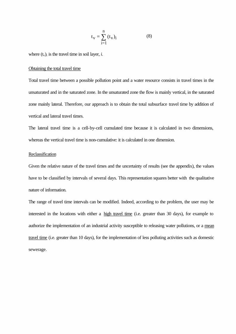
t tv v ii

n=

=∑ ( )

1

(8)

where (tv)i is the travel time in soil layer, i.

Obtaining the total travel time

Total travel time between a possible pollution point and a water resource consists in travel times in the

unsaturated and in the saturated zone. In the unsaturated zone the flow is mainly vertical, in the saturated

zone mainly lateral. Therefore, our approach is to obtain the total subsurface travel time by addition of

vertical and lateral travel times.

The lateral travel time is a cell-by-cell cumulated time because it is calculated in two dimensions,

whereas the vertical travel time is non-cumulative: it is calculated in one dimension.

Reclassification

Given the relative nature of the travel times and the uncertainty of results (see the appendix), the values

have to be classified by intervals of several days. This representation squares better with the qualitative

nature of information.

The range of travel time intervals can be modified. Indeed, according to the problem, the user may be

interested in the locations with either a high travel time (i.e. greater than 30 days), for example to

authorize the implementation of an industrial activity susceptible to releasing water pollutions, or a mean

travel time (i.e. greater than 10 days), for the implementation of less polluting activities such as domestic

sewerage.

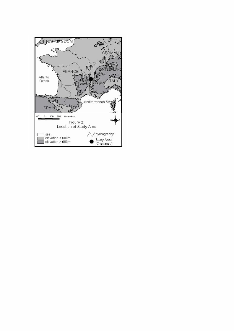
APPLICATION TO AN AREA IN THE EAST OF MASSIF CENTRAL (FRANCE): THE

GRANITIC PIEDMONT OF PELUSSIN AND THE ALLUVIAL PLAIN OF CHAVANAY

This area covers 55 km² and is situated in the Rhône Valley (Figure 2). The Rhône River is associated

with an aquifer in the alluvial plain of Chavanay. This aquifer is exploited by some wells for irrigation and

drinking water supply. Aquifer is recharged by the Rhône river and some small rivers which drain the

granitic piedmont.

The study area is intensively occupied by several villages, and exploited by fruit growing in the alluvial

plain, pasture and vineyard in the granitic piedmont. Furthermore, it is crossed by a national road and a

railway. In 1990, a railway accident caused severe hydrocarbon pollution which threatened the drinking

water wells in the alluvial aquifer. From this event, it has been concluded that it is necessary to improve

the protection of the water resources in this area.

Data available

The geological map of Bureau de Recherche Géologique et Minières (BRGM, 1970) have been

digitalized for granitic piedmont, we have completed this map by field observations in order to map the

areas without soil cover. For alluvial areas, we have digitalized a piezometric map and the location of

wells (Pierlay and de Bellegarde, 1986).

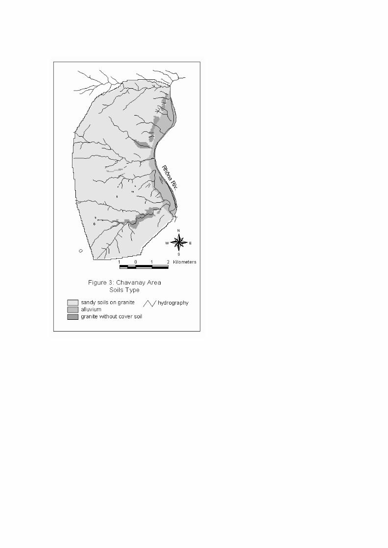
For each soil type (Figure 3), we have assigned two values of porosity and hydraulic conductivity (one

for top layer and another for bottom layer) which depend on texture (from the table of Rawls and

Brakensiek, 1985) and structure.

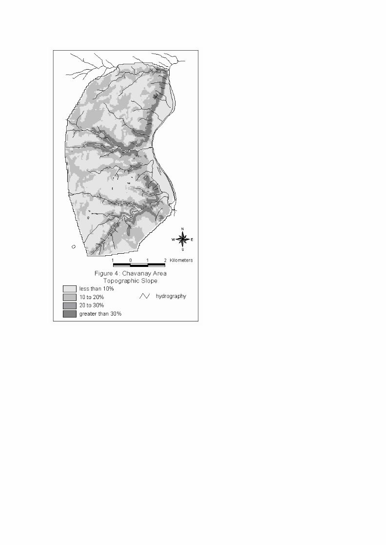
The contours of the topographic map of Institut de Géographie National (IGN, 1990) have been

digitized. We have interpolated the vector map by a Triangulated Irregular Network, then we have

rasterized the result to obtain a Digital Elevation Model (DEM). Some corrections of the DEM have

been necessary to simulate the flow (Jenson and Domingue, 1988). The west of the study area is more

uneven than the flat alluvial plain in the east (Figure 4).

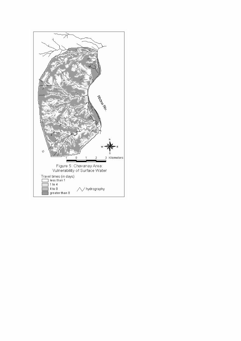
Superficial Water Vulnerability Map (Figure 5)

The resulting map shows two types of functioning. It implies different decision strategies for activities

with a risk of pollution.

The travel times are very variable on this area. The shallow and sandy soils and the high slopes in the

western granitic piedmont are responsible for great flow velocities, whereas, in the eastern part, the

permeable alluvial plain allows an infiltration into the alluvial aquifer and a slower transfer to the river.

River quality protection must be strengthened in the granitic piedmont and activities with potential

pollution must be located only in areas with a sufficient travel time to the rivers.

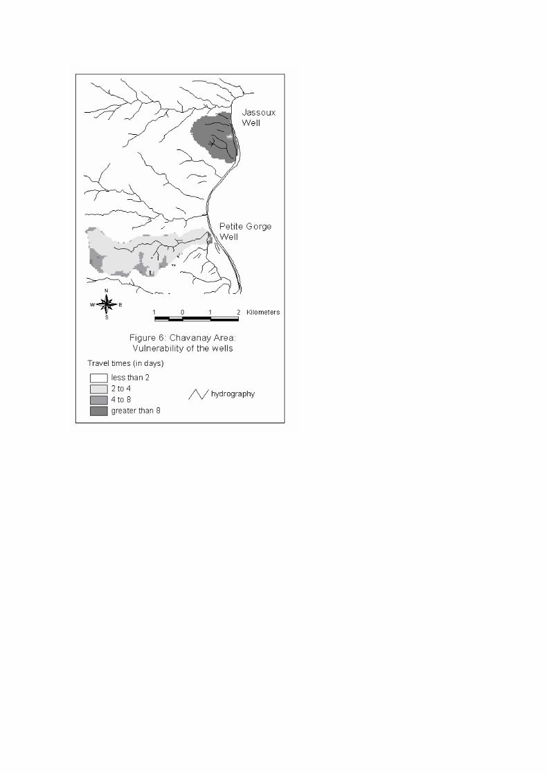
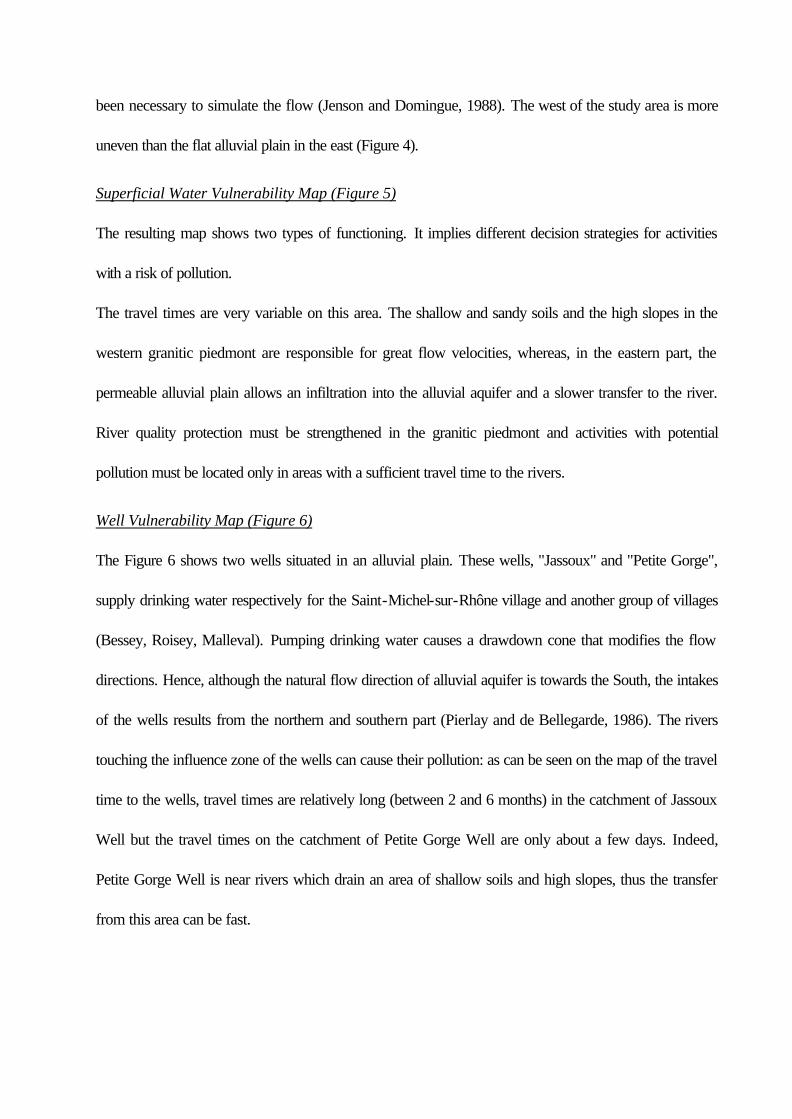
Well Vulnerability Map (Figure 6)

The Figure 6 shows two wells situated in an alluvial plain. These wells, "Jassoux" and "Petite Gorge",

supply drinking water respectively for the Saint-Michel-sur-Rhône village and another group of villages

(Bessey, Roisey, Malleval). Pumping drinking water causes a drawdown cone that modifies the flow

directions. Hence, although the natural flow direction of alluvial aquifer is towards the South, the intakes

of the wells results from the northern and southern part (Pierlay and de Bellegarde, 1986). The rivers

touching the influence zone of the wells can cause their pollution: as can be seen on the map of the travel

time to the wells, travel times are relatively long (between 2 and 6 months) in the catchment of Jassoux

Well but the travel times on the catchment of Petite Gorge Well are only about a few days. Indeed,

Petite Gorge Well is near rivers which drain an area of shallow soils and high slopes, thus the transfer

from this area can be fast.

Validation of transfer times against piezometric data

For an exact validation of the model, it would be necessary to measure an experimental travel time.

However not having these measurements, the validation of our method is restricted by the limited nature

of the available data.

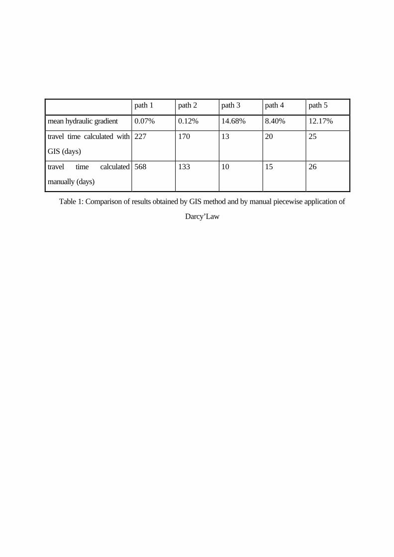
In order to test the proposed algorithm of backtracing for a zoning of transfer times, we have compared

the results of this zoning method to piecewise application of Darcy’s Law to piezometric level data,

following the subsurface flow (Table 1).

The travel times are close between both methods when the gradient is not too low as on the western

slopes (paths 3 to 5). In alluvial plain, however, the results can vary by twice as much between both

methods (paths 1 and 2). The ARC/INFO algorithm, pathdistance or focal spreading in function

(Tomlin, 1990), seems to be unsuitable when the surface is too flat. In such cases, the results must be

taken cautiously.

It should be emphasized that a validation by field measurments must give different results than the

calculation: indeed, as we can see in the Appendix, the model is highly sensitive to hydraulic conductivity

and hydraulic gradient, two parameters known with a low accuracy.

Further work

The present work shows a method which starts from the location of a water resource which has to be

protected. We have traced back the shortest way of a potential pollutant. If we have presented an

"upstream model approach", further work will take into account the complementary approach, regarding

a pollutant which is released at some arbitrary point and previewing its way, travel times and spreading

behaviour in a porous medium. By this approach, we can link GIS with hydrodispersive models based

on differential equations such as flow and dispersion equation. The results of flow and dispersion

calculations can be evaluated in a similiar way as in the approach proposed here.

CONCLUSION

A method for estimating water resources vulnerability to pollution has been presented. The method

consists of a zoning of a given study area for a relative vulnerability of one zone to another. Absolute

travel times can be included but have to be handled with care.

For this, the influencing parameters for the different runoff mechanisms and their spatial distribution have

been studied. Calculation of cost estimation by the inverse of transfer velocity and multiplying with

transfer distance yields reasonable results for transfer times as compared with traditional methods.

Relative zoning is useful to prescribe the impacts of a potential pollutant activity. For studying more

detailed transfer mechanisms of pollutants, it is possible to couple this tool to more specific models

which can take into account other phenomena such as dispersion, adsorption phenomena and bio-

degradation.

APPENDIX: ERRORS AND ERROR PROPAGATION

The calculation of transfer velocity in aquifer and subsurface is based on Darcy’s Law (equation (1)).

The estimation of velocity error needs estimation of the error of the parameters intervening in this law.

Each parameter x can be expressed by a mean value x and a standard deviation σx:

x = x ± σx (9)

We obtain the following expressions:

Hydraulic conductivity k: a logarithmic error is assumed equal to (log 5) on the mean hydraulic

conductivity:

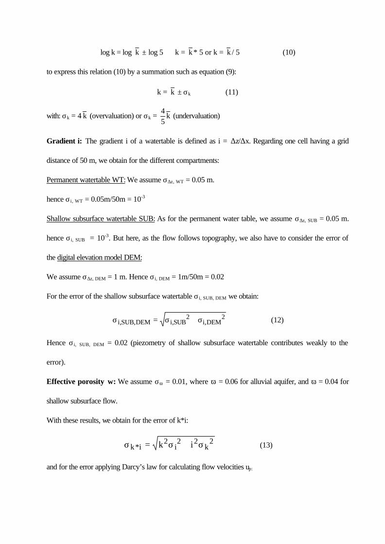
log k = log k ± log 5 ⇔ k = k * 5 or k = k / 5 (10)

to express this relation (10) by a summation such as equation (9):

k = k ± σk (11)

with: σk = 4 k (overvaluation) or σk = 45

k (undervaluation)

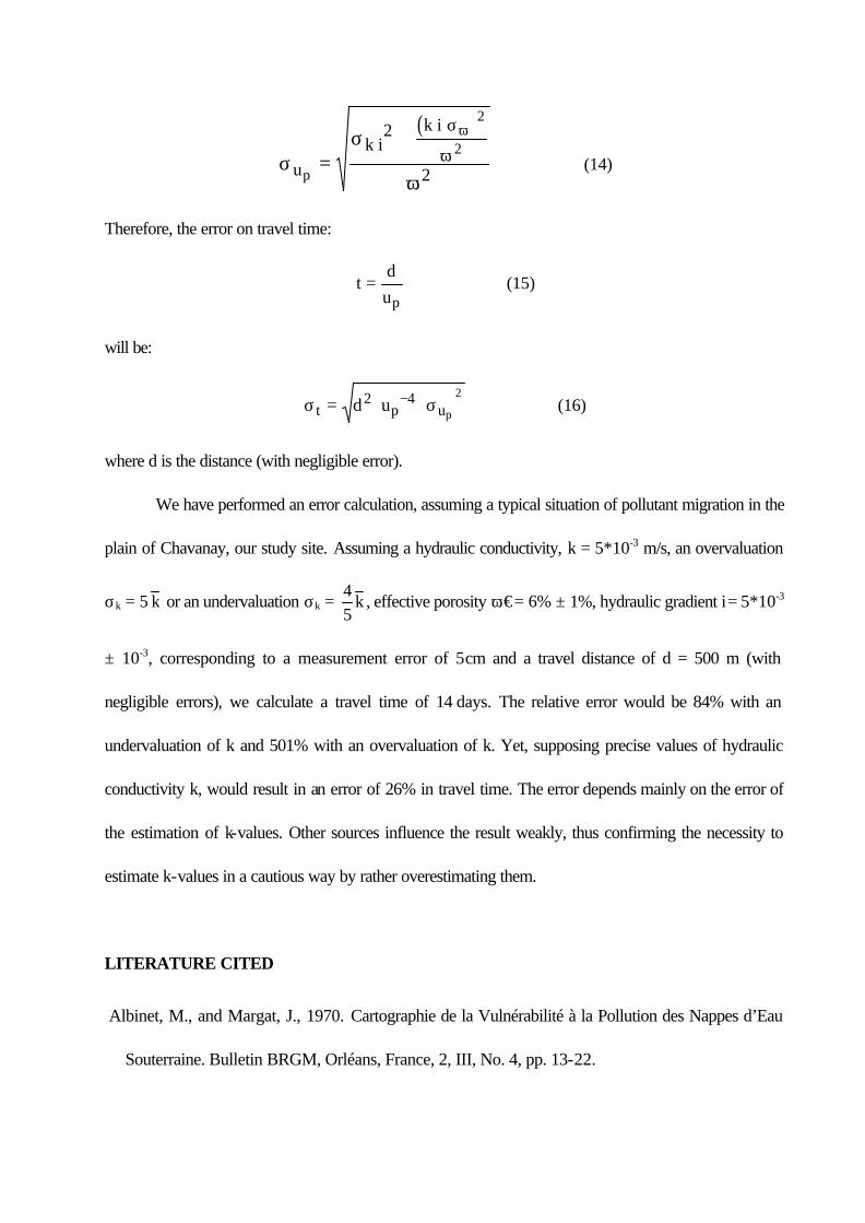
Gradient i: The gradient i of a watertable is defined as i = ∆z/∆x. Regarding one cell having a grid

distance of 50 m, we obtain for the different compartments:

Permanent watertable WT: We assume σ∆z, WT = 0.05 m.

hence σi, WT = 0.05m/50m = 10-3

Shallow subsurface watertable SUB: As for the permanent water table, we assume σ∆z, SUB = 0.05 m.

hence σi, SUB = 10-3. But here, as the flow follows topography, we also have to consider the error of

the digital elevation model DEM:

We assume σ∆z, DEM = 1 m. Hence σi, DEM = 1m/50m = 0.02

For the error of the shallow subsurface watertable σi, SUB, DEM we obtain:

σ σ σi SUB DEM i SUB i DEM, , , ,= +2 2 (12)

Hence σi, SUB, DEM = 0.02 (piezometry of shallow subsurface watertable contributes weakly to the

error).

Effective porosity ω: We assume σω = 0.01, where ω = 0.06 for alluvial aquifer, and ω = 0.04 for

shallow subsurface flow.

With these results, we obtain for the error of k*i:

σ σ σk i i kk i* = +2 2 2 2 (13)

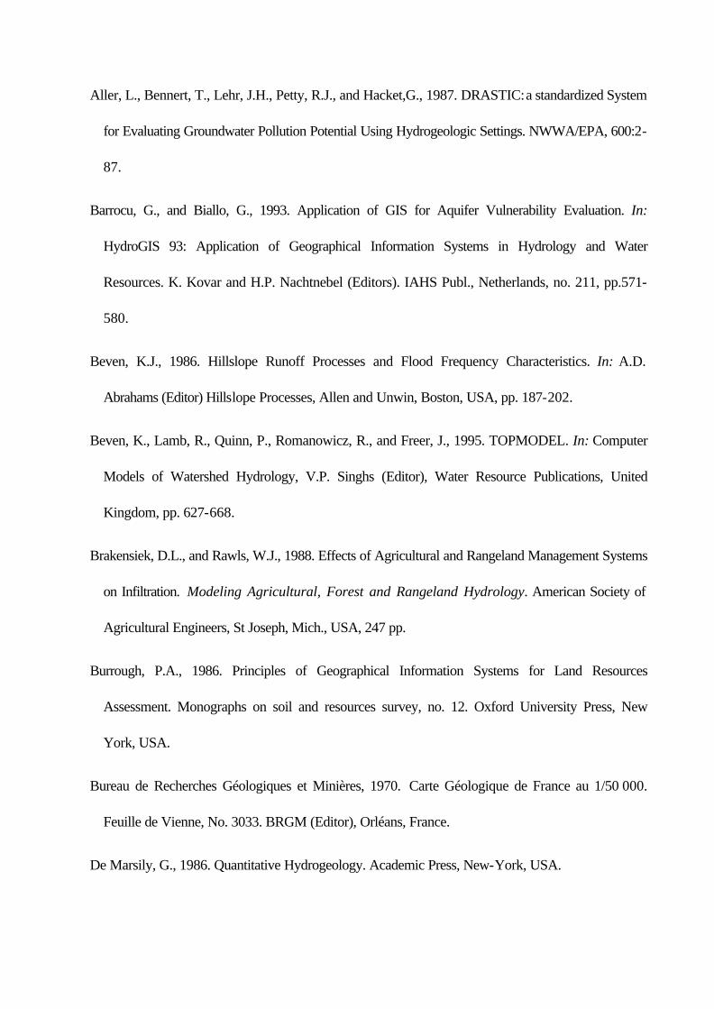
and for the error applying Darcy’s law for calculating flow velocities up:

( )

σσ

ω

ω

ωu

k ik i

p=

+⋅⋅ ⋅σ2

2

2

2 (14)

Therefore, the error on travel time:

tdup

= (15)

will be:

σ σt p ud up

= ⋅ ⋅−2 4 2 (16)

where d is the distance (with negligible error).

We have performed an error calculation, assuming a typical situation of pollutant migration in the

plain of Chavanay, our study site. Assuming a hydraulic conductivity, k = 5*10-3 m/s, an overvaluation

σk = 5 k or an undervaluation σk = 45

k , effective porosity ω€= 6% ± 1%, hydraulic gradient i = 5*10-3

± 10-3, corresponding to a measurement error of 5 cm and a travel distance of d = 500 m (with

negligible errors), we calculate a travel time of 14 days. The relative error would be 84% with an

undervaluation of k and 501% with an overvaluation of k. Yet, supposing precise values of hydraulic

conductivity k, would result in an error of 26% in travel time. The error depends mainly on the error of

the estimation of k-values. Other sources influence the result weakly, thus confirming the necessity to

estimate k-values in a cautious way by rather overestimating them.

LITERATURE CITED

Albinet, M., and Margat, J., 1970. Cartographie de la Vulnérabilité à la Pollution des Nappes d’Eau

Souterraine. Bulletin BRGM, Orléans, France, 2, III, No. 4, pp. 13-22.

Aller, L., Bennert, T., Lehr, J.H., Petty, R.J., and Hacket,G., 1987. DRASTIC: a standardized System

for Evaluating Groundwater Pollution Potential Using Hydrogeologic Settings. NWWA/EPA, 600:2-

87.

Barrocu, G., and Biallo, G., 1993. Application of GIS for Aquifer Vulnerability Evaluation. In:

HydroGIS 93: Application of Geographical Information Systems in Hydrology and Water

Resources. K. Kovar and H.P. Nachtnebel (Editors). IAHS Publ., Netherlands, no. 211, pp.571-

580.

Beven, K.J., 1986. Hillslope Runoff Processes and Flood Frequency Characteristics. In: A.D.

Abrahams (Editor) Hillslope Processes, Allen and Unwin, Boston, USA, pp. 187-202.

Beven, K., Lamb, R., Quinn, P., Romanowicz, R., and Freer, J., 1995. TOPMODEL. In: Computer

Models of Watershed Hydrology, V.P. Singhs (Editor), Water Resource Publications, United

Kingdom, pp. 627-668.

Brakensiek, D.L., and Rawls, W.J., 1988. Effects of Agricultural and Rangeland Management Systems

on Infiltration. Modeling Agricultural, Forest and Rangeland Hydrology. American Society of

Agricultural Engineers, St Joseph, Mich., USA, 247 pp.

Burrough, P.A., 1986. Principles of Geographical Information Systems for Land Resources

Assessment. Monographs on soil and resources survey, no. 12. Oxford University Press, New

York, USA.

Bureau de Recherches Géologiques et Minières, 1970. Carte Géologique de France au 1/50 000.

Feuille de Vienne, No. 3033. BRGM (Editor), Orléans, France.

De Marsily, G., 1986. Quantitative Hydrogeology. Academic Press, New-York, USA.

Institut de Géographie National, 1990. Carte Topographique au 1 / 25 000, feuille de Roussillion, No.

3033 ouest. IGN, Paris, France.

Jenson, S.K., and Domingue, J.O., 1988. Extracting Topographic Structure from Digital Elevation

Data for Geographic System Analysis. Photogrammetric Engineering and Remote Sensing, 54,

11:1593-1600.

Kirkby M.J., 1975. Hydrograph Modelling Strategies. In: Process in Physical and Human Geography,

R. Peel, M. Chisholm and P. Hagget (Editors), Heinemann, United Kingdom, pp. 69-90.

La Berbera, P., Lanza, L., and Siccardi, F., 1993. Hydrologically Oriented GIS and Application to

Rainfall-Runoff Distributed Modelling: Case Study of Arno Basin. In: HydroGIS 93: Application of

Geographical Information Systems in Hydrology and Water Resources. K. Kovar and H.P.

Nachtnebel (Editors). IAHS Publ., Netherlands, no. 211, pp. 171-179.

Lallemand-Barrès, A., and Roux, J.C., 1989. Guide Méthodologique d'Etablissement des Périmètres

de Protection des Captages d'Eau Souterraine Destinée à la Consommation Humaine. Ed. BRGM,

no. 19, Orléans, France.

Laurent, F., 1996. Outils de modélisation spatiale pour la gestion intégrée des ressources en eau -

Application aux Schémas d’Aménagement et de Gestion des Eaux. Thesis, Ecole des Mines de

Paris, Ecole des Mines de Saint-Etienne, France, 357 pp.

Laurent, F., Graillot, D., and Déchomets, R., 1995. Rivers and Groundwater vulnerability to

Accidental Pollution. Spatial Analysis of Vulnerability Areas. In: TIEMEC, May 9-12, 1995, Nice,

France, Sullivan, J.D., J.C. Wybo and L. Buisson (Editors), pp. 451-458.

Maidment, D., 1993. GIS and Hydrologic Modelling. In: Environmental Modelling with GIS, Oxford

University Press, United Kingdom, pp. 147-167.

Maidment, D., 1996. Environmental Modeling within GIS. In: GIS and Environmental Modeling:

progress and research issues, Goodchild M. et al. (Editors), Fort Collins, USA, pp. 315-324.

Moore, I.D., Grayson, R.B., and Ladson, A.R., 1991. Digital Terrain Modelling: a review of

hydrological, geomorphological and biological applications. Hydrological Processes, 5: 3-30.

Munoz, S., and Langevin, C., 1991. Adaptation d’une Méthode Cartographique Assistée à

l’Elaboration des Cartes de Vulnérabilité au Guatemala. Hydrogéologie, BRGM, Orléans, France,

No. 1, pp. 65-84.

Navulur, K., and Engel, B., 1996. Predicting Spatial Distributions of Vulnerability of Indiana State

Aquifer Systems to Nitrate Leaching using a GIS. In: Proceedings, Third International

Conference/Workshop on Integrating GIS and Environmental Modeling, Santa Fe, NM, USA,

January 21-26, 1996. Santa Barbara, CA, USA: National Center for Geographic Information and

Analysis. http://www.ncgia.ucsb.edu/conf/SANTA_FE_CD-ROM/main.html.

O’Callaghan, J.F., and Mark, D.M., 1984. The Extraction of Drainage Network from Digital Elevation

Data. Computers Vision Graphics and Image Processing, 28:323-344.

Peverieri, G., Fico, L., Suppo, M., and Crema, G., 1991. Utilization of a Geographic Information

System for Study, Conservation and Management of Groundwater Resources in the Ofanto River

(Italy). Hydrogéologie, BRGM, Orléans, France, No. 1, pp. 11-24.

Pierlay, B., and de Bellegarde, B., 1986. Nappe de la Plaine de Chavanay (42), Puits de la "Petite

Gorge": Etude de la Pollution par le Fer et le Manganèse. Service Régional d’Aménagement des

Eaux Rhône-Alpes, Lyon, France, No. 3-HYD-1986.

Pilgrim, D.H., and Cordery, I., 1992. Flood Runoff. In: Handbook of Hydrology, Maidment, D.R.

(Editor). Mc Graw-Hill, Inc., USA, pp. 9.1-9.42.

Quinn, P., 1991. The role of Digital Terrain Analysis in Hydrological Modelling. PhD, Environmental

Sciences Division, Lancaster University, Lancaster, United Kingdom.

Quinn, P., Beven, K., Chevallier, P., and Planchon, O., 1991. The Prediction of Hillslope Flow Paths

for Distributed Hydrological Modelling using Digital Terrain Models. Hydrological Processes 5:59-

79.

Rawls, W.J., and Brakensiek, D.L., 1983. A Procedure to Predict Green Ampt Infiltration Parameters.

Adv. Infiltration, American Society of Agricultural Engineers, pp. 102-112.

Rawls, W.J., and Brakensiek, D.L., 1985. Prediction of Soil Water Properties for Hydrologic

Modeling. Watershed Management in the Eighties, ASCE, pp.293-299.

Richert, J.E., Young, S.E., and Johnson, C., 1992. SEEPAGE: a GIS model for groundwater pollution

potential. In: ASAE 1992 International Winter Meeting, Nashville, Tennessee, 15-18 dec. 1992,

Paper No. 922592.

Saxton, K.E., Rawls, W.J., Romberger, J.S., and Papendick, R.I., 1986. Estimating Generalized Soil-

Water Characteristics from Texture. American Society of Agricultural Engineers, St Joseph, Mich.,

USA, 50, 4, pp. 1031-1035.

Skaggs, R.W., and Khaleel, R., 1982. Infiltration. Hydrologic Modeling of Small Watersheds,

Monograph 5, C.T. Haan (Editor). American Society of Agricultural Engineers, St Joseph, Mich.,

USA, pp. 4-166.

Snyder, D.T., and Wilkinson, J.M., 1992. Use of a Ground-water Flow Model With Particle Tracking

to Evaluate Aquifer Vulnerability. In: American Geophysical Union Fall Meeting, 12/7-11/92, San

Francisco, CA, USA, p. 217.

Tomlin, C.D., 1990. Geographic Information Systems and Cartographic Modeling. Prentice-Hall,

Englewood Cliffs, USA.

Vested, H.J., Justesen, P., and Ekebjaerg, L., 1992. Advection-Dispersion Modelling in Three

Dimensions. Applied Mathematical Modelling 16:506-519.

path 1 path 2 path 3 path 4 path 5

mean hydraulic gradient 0.07% 0.12% 14.68% 8.40% 12.17%

travel time calculated with

GIS (days)

227 170 13 20 25

travel time calculated

manually (days)

568 133 10 15 26

Table 1: Comparison of results obtained by GIS method and by manual piecewise application of

Darcy’Law

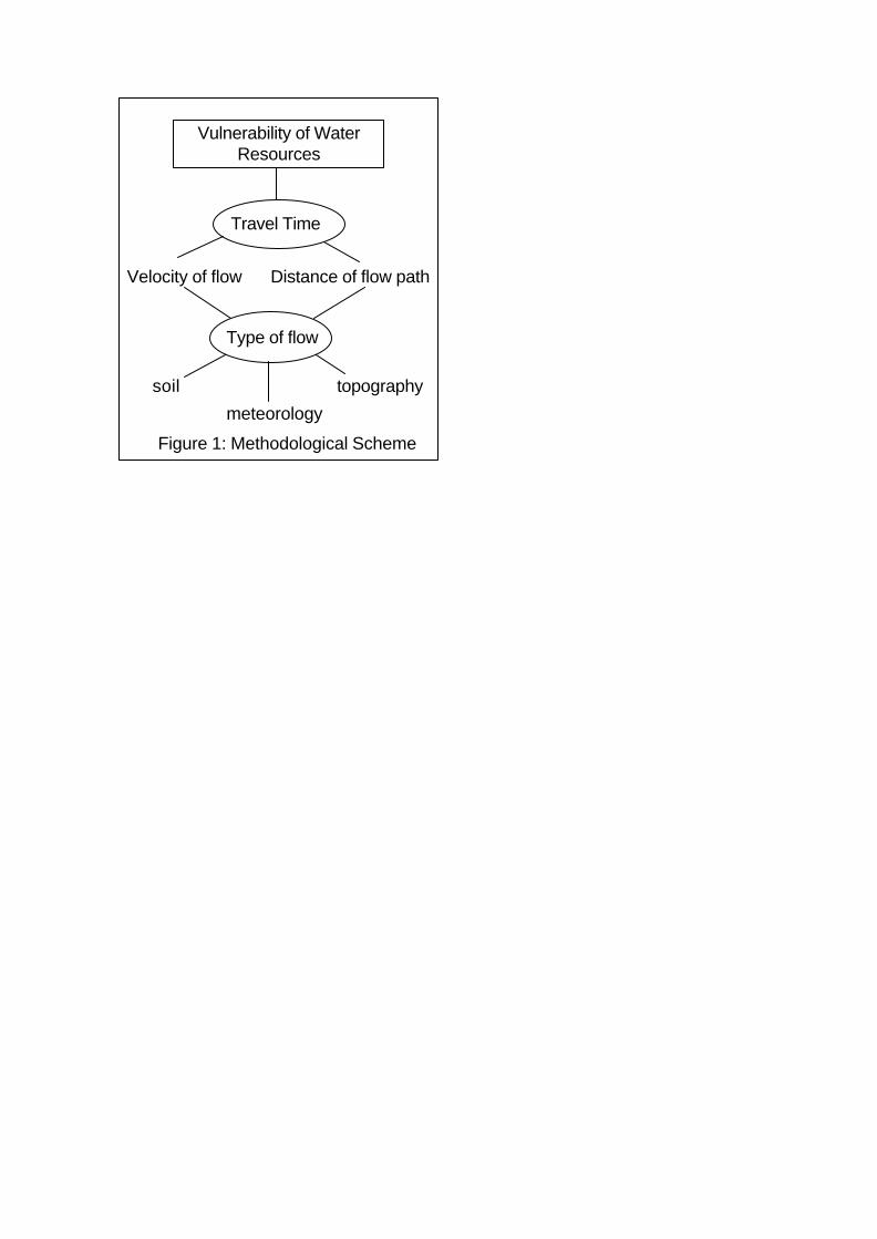
Vulnerability of Water Resources

Travel Time

Velocity of flow Distance of flow path

Type of flow

soil

meteorology

topography

Figure 1: Methodological Scheme