Case-based modification for optimization agents: AGENT-OPT

Case-based modification for optimization agents: AGENT-OPT

Yong Sik Changa, Jae Kyu Leeb,*

a International Center for Electronic Commerce, 207-43, Cheongryang, Seoul 130-012, South KoreabGraduate School of Management, Korea Advanced Institute of Science and Technology, 207-43, Cheongryang, Seoul 130-012, South Korea

Abstract

For the effective implementation of an inter-organizational supply chain on the Web, many optimization model agents need

to be embedded in the distributed software agents. For instance, many suppliers make requests to a delivery scheduler who

manages a model warehouse at the e-hub. The scheduler deals with the scheduling of many truckers and each trucker’s agent

must have its own routing optimization models. Since the formulations in the model warehouse vary depending upon the

requirements, it is impossible to formulate all combinations in advance. Therefore, we need a case-based model modification

scheme that can generate the required formulation from the semantically specified requirement in the agent communication

language.

This research deals with the issues of the architecture of an optimization model agent system AGENT-OPT, modeling

request language in XML, optimization model representation in semantic-level objects using UNIK-OPT, a method of selecting

a base model, an optimization model modification language (OMML), and rule-based modification reasoning. The approach is

applied to the delivery scheduling to study the effect of base model selection policies on the modification effort. To determine

whether to start with a primitive model, full model, or the most similar model, we experimented with the sensitivity of proximity

to the primitive model on 24 cases and discovered the threshold for choosing the most efficient base model.

D 2003 Elsevier B.V. All rights reserved.

Keywords: Agent; Case-based model formulation; Optimization; Delivery scheduling; Supply chain

1. Introduction

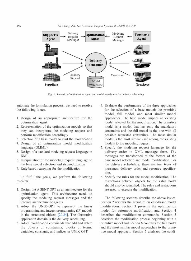
For the effective implementation of an inter-organ-

izational supply chain on the Web, many optimization

models need to be embedded in distributed software

agents. For instance, when there are many suppliers

that need delivery from a group of truckers, we need a

third party to schedule the optimal delivery for truck-

ers and suppliers. Since each delivery may have dif-

ferent requirements, the predefined models may not be

able to cover the variety of modeling requests from

the suppliers. Consequently, the third party delivery

scheduler needs to maintain a model warehouse [6]

with the capability to formulate the optimization

model based on the modeling request specified in

XML messages, see Fig. 1.

Since it is reasonable to assume that the scheduler

has some predefined models, we can apply the case-

based modification approach for the formulation of

models. Our primary concern here is how to automate

the modification process effectively and efficiently. To

0167-9236/$ - see front matter D 2003 Elsevier B.V. All rights reserved.

doi:10.1016/S0167-9236(03)00026-5

* Corresponding author. Tel.: +82-2-958-3612; fax: +82-2-960-

2102.

E-mail addresses: [email protected] (Y.S. Chang),

[email protected] (J.K. Lee).

www.elsevier.com/locate/dsw

Decision Support Systems 36 (2004) 355–370

automate the formulation process, we need to resolve

the following issues.

1. Design of an appropriate architecture for the

optimization agent

2. Representation of the optimization models so that

they can incorporate the modeling request and

perform modification accordingly

3. Selection of a base model to start the modification

4. Design of an optimization model modification

language (OMML)

5. Design of a standard modeling request language in

XML

6. Interpretation of the modeling request language to

the base model selection and its modification

7. Rule-based reasoning for the modification

To fulfill the goals, we perform the following

research.

1. Design the AGENT-OPT as an architecture for the

optimization agent. This architecture needs to

specify the modeling request messages and the

internal architecture of agents.

2. Adopt the UNIK-OPT to represent the linear

programming and integer programming (IP) models

in the structured objects [20,24]. The illustrative

application domain is the delivery scheduling.

3. Adopt modification commands that add and delete

the objects of constraints, blocks of terms,

variables, constants, and indices in UNIK-OPT.

4. Evaluate the performance of the three approaches

for the selection of a base model: the primitive

model, full model, and most similar model

approaches. The base model implies an existing

model selected for the modification. The primitive

model is a model that has only the mandatory

constraints and the full model is the one with all

possible requested constraints. The most similar

model is the most similar case among the existing

models to the modeling request.

5. Specify the modeling request language for the

delivery order in XML message form. The

messages are transformed to the factors of the

base model selection and model modification. For

the delivery scheduling, there are two types of

messages: delivery order and resource specifica-

tion.

6. Specify the rules for the model modification. The

restrictions between objects for the valid model

should also be identified. The rules and restrictions

are used to execute the modification.

The following sections describe the above issues.

Section 2 reviews the literature on case-based model

modification. Section 3 presents the optimization

model for automatic modification and Section 4

describes the modification commands. Section 5

describes the modification process beginning with a

primitive model and Section 6 contrasts the full model

and the most similar model approaches to the primi-

tive model approach. Section 7 analyzes the condi-

Fig. 1. Scenario of optimization agent and model warehouse for delivery scheduling.

Y.S. Chang, J.K. Lee / Decision Support Systems 36 (2004) 355–370356

tions when an approach is most efficient. Section 8

describes the architecture of AGENT-OPT that adopts

the proposed approaches.

2. Literature on case-based model formulations

There is a considerable amount of research on

model management systems (MMS) [5,11] that sup-

ports the various phases of the modeling life-cycle.

The importance of MMS is resurrected as the necessity

for a model warehouse arises in the Web-based hub

[6]. Earlier research studied the representations of

models and the reasoning methods in order to map

specific problems with the model structure.

From the perspective of data and object manage-

ment, network data modeling [18], relational data

modeling [3], entity-relationship data modeling [4],

and object-oriented data modeling [14,21,30,35]

approaches were attempted. Liang proposed a frame-

work that included both relational and network con-

cepts [31]. On the other hand, from the perspective of

Artificial Intelligence, researchers adopted knowledge

representation techniques to represent models and

focused on automating the modeling processes. These

representations are based on predicate calculus [7],

semantic information net [11], knowledge abstraction

[9], first order logic [10,19], structured modeling

[12,13,36,38], rule-based formulation [23,28], and

frame [2,20,22,24].

It is very difficult to formulate a model from

scratch. It is reasonable, therefore, to modify the

existing models on the case-based reasoning approach.

Case-based planning was proposed by Vellore et al.

[39]. Modeling by analogy was researched by Blan-

ning [3], Ishikawa and Terano [15], Kedar-Cabelli

[16], Liang [32], Liang and Konsynski [34], and

Winston [40]. Both analogical and case-based reason-

ing methods rely on encapsulating episodic knowledge

to guide complex problem solving. The former empha-

sizes the process of modification, adaptation and

derivation, whereas the latter emphasizes the organ-

ization, hierarchy indexing and retrieval of case mem-

ory [8]. Modeling by analogy builds a new model

through feature mapping on conceptual, structural, and

functional similarities. However, it is not efficient

when modification of the model structure is required.

As Liang pointed out, this approach is relatively rigid

and the computational cost may be excessive partic-

ularly when large-scaled, because feature mapping is

theoretically NP-complete [33]. Instead of mapping a

new problem to the stored model counterpart, Binba-

sioglu [1] proposed the process analogy approach.

This approach designs a model without model struc-

ture modification from reusable model pieces. Never-

theless, it is rare for stored models to be reused without

structural modification.

Therefore, we need a more flexible and efficient

method that will automatically modify the models. In

this study, we adopt UNIK-OPT [24], which repre-

sents the optimization models—both the linear and

integer programming models—in structured objects.

Since the underlying design principle of UNIfied

Knowledge (UNIK) was the representation of opti-

mization models so as to integrate with rules [27], its

object-oriented representation is suitable for modifi-

cation. The earlier versionUNIK-LP, which focused on

the linear programming, did not assist the eXclusive

OR (XOR) relationship of variables and the IF–THEN

relationships between constraints. These higher-level

representations mean it should be extended to integer

programming models, thus the system UNIK-IP [41]

was developed. UNIK-RELAX [17] was also devel-

oped to identify the characteristics of model structure

and to plan the Lagrangian relaxation procedure to

solve IP models.

3. Representation of optimization model

formulation in objects

To apply the CBR approach to the optimization

model formulation, we need to represent the model

cases in such a way that they semantically understand

the modeling requests and modification commands.

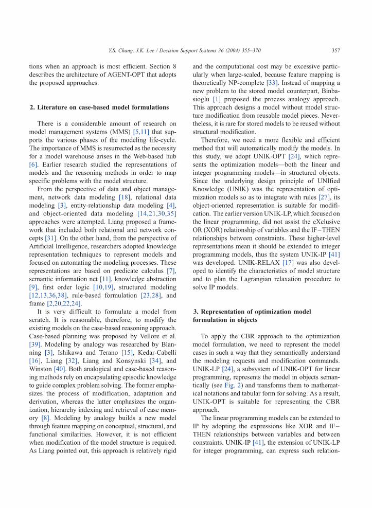
UNIK-LP [24], a subsystem of UNIK-OPT for linear

programming, represents the model in objects seman-

tically (see Fig. 2) and transforms them to mathemat-

ical notations and tabular form for solving. As a result,

UNIK-OPT is suitable for representing the CBR

approach.

The linear programming models can be extended to

IP by adopting the expressions like XOR and IF–

THEN relationships between variables and between

constraints. UNIK-IP [41], the extension of UNIK-LP

for integer programming, can express such relation-

Y.S. Chang, J.K. Lee / Decision Support Systems 36 (2004) 355–370 357

ships and transform them to valid integer program-

ming model formulations for IP solvers.

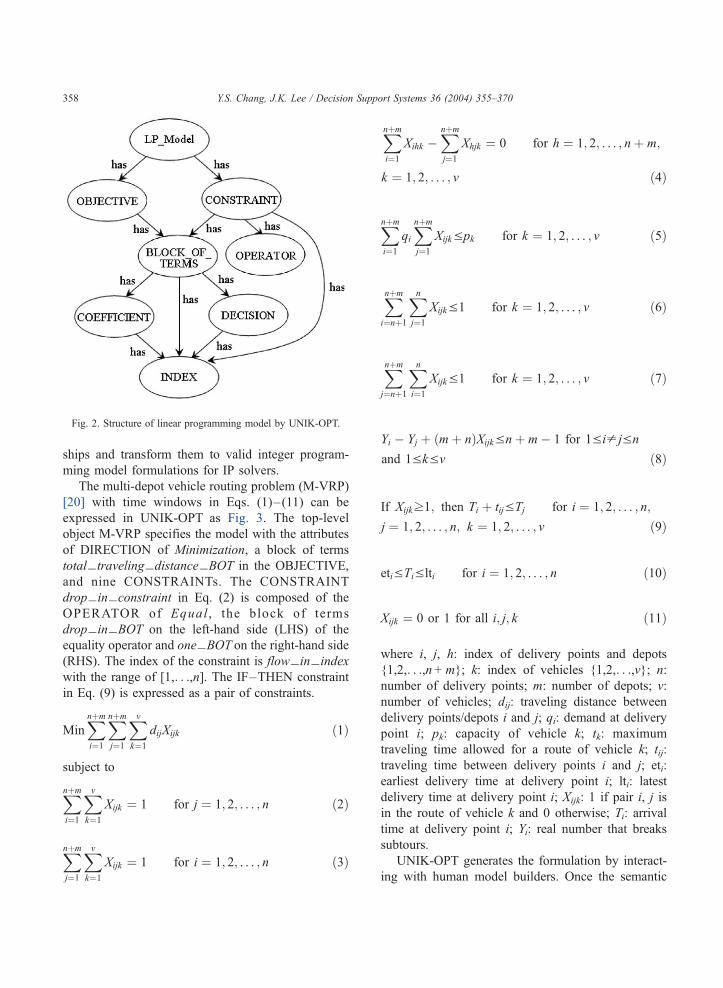
The multi-depot vehicle routing problem (M-VRP)

[20] with time windows in Eqs. (1)–(11) can be

expressed in UNIK-OPT as Fig. 3. The top-level

object M-VRP specifies the model with the attributes

of DIRECTION of Minimization, a block of terms

total�traveling�distance�BOT in the OBJECTIVE,

and nine CONSTRAINTs. The CONSTRAINT

drop�in�constraint in Eq. (2) is composed of the

OPERATOR of Equal , the block of terms

drop�in�BOT on the left-hand side (LHS) of the

equality operator and one�BOT on the right-hand side

(RHS). The index of the constraint is flow�in�index

with the range of [1,. . .,n]. The IF–THEN constraint

in Eq. (9) is expressed as a pair of constraints.

MinXnþm

i¼1

Xnþm

j¼1

Xv

k¼1

dijXijk ð1Þ

subject to

Xnþm

i¼1

Xv

k¼1

Xijk ¼ 1 for j ¼ 1; 2; . . . ; n ð2Þ

Xnþm

j¼1

Xv

k¼1

Xijk ¼ 1 for i ¼ 1; 2; . . . ; n ð3Þ

Xnþm

i¼1

Xihk �Xnþm

j¼1

Xhjk ¼ 0 for h ¼ 1; 2; . . . ; nþ m;

k ¼ 1; 2; . . . ; v ð4Þ

Xnþm

i¼1

qiXnþm

j¼1

XijkVpk for k ¼ 1; 2; . . . ; v ð5Þ

Xnþm

i¼nþ1

Xn

j¼1

XijkV1 for k ¼ 1; 2; . . . ; v ð6Þ

Xnþm

j¼nþ1

Xn

i¼1

XijkV1 for k ¼ 1; 2; . . . ; v ð7Þ

Yi � Yj þ ðmþ nÞXijkVnþ m� 1 for 1Vi p jVn

and 1VkVv ð8Þ

If Xijkz1; then Ti þ tijVTj for i ¼ 1; 2; . . . ; n;

j ¼ 1; 2; . . . ; n; k ¼ 1; 2; . . . ; v ð9Þ

etiVTiVlti for i ¼ 1; 2; . . . ; n ð10Þ

Xijk ¼ 0 or 1 for all i; j; k ð11Þ

where i, j, h: index of delivery points and depots

{1,2,. . .,n+m}; k: index of vehicles {1,2,. . .,v}; n:

number of delivery points; m: number of depots; v:

number of vehicles; dij: traveling distance between

delivery points/depots i and j; qi: demand at delivery

point i; pk: capacity of vehicle k; tk: maximum

traveling time allowed for a route of vehicle k; tij:

traveling time between delivery points i and j; eti:

earliest delivery time at delivery point i; lti: latest

delivery time at delivery point i; Xijk: 1 if pair i, j is

in the route of vehicle k and 0 otherwise; Ti: arrival

time at delivery point i; Yi: real number that breaks

subtours.

UNIK-OPT generates the formulation by interact-

ing with human model builders. Once the semantic

Fig. 2. Structure of linear programming model by UNIK-OPT.


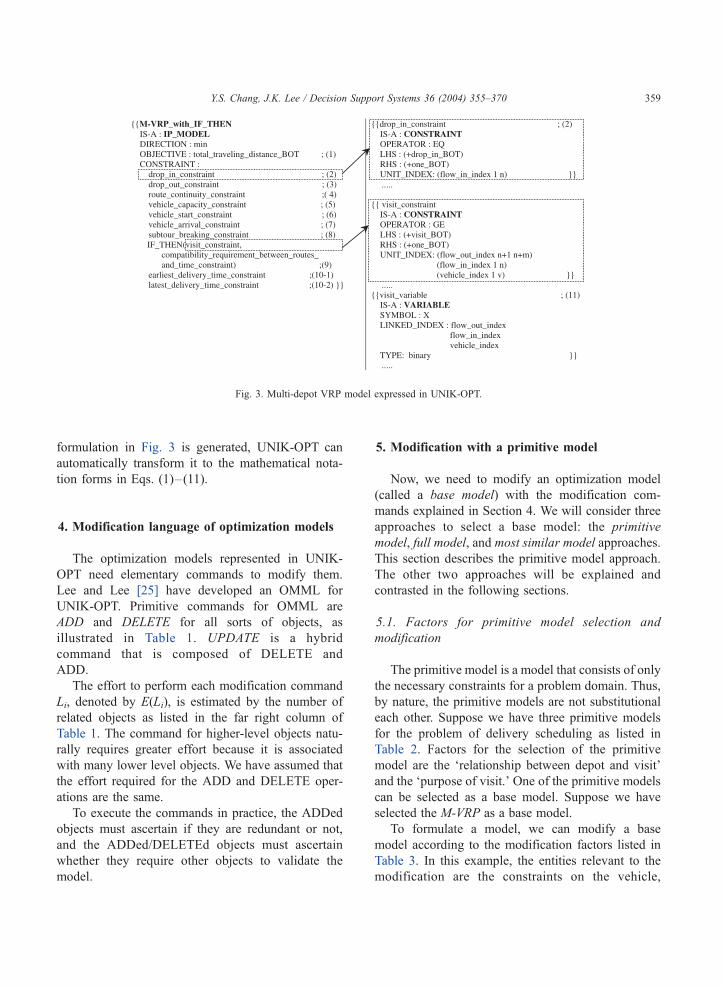
formulation in Fig. 3 is generated, UNIK-OPT can

automatically transform it to the mathematical nota-

tion forms in Eqs. (1)–(11).

4. Modification language of optimization models

The optimization models represented in UNIK-

OPT need elementary commands to modify them.

Lee and Lee [25] have developed an OMML for

UNIK-OPT. Primitive commands for OMML are

ADD and DELETE for all sorts of objects, as

illustrated in Table 1. UPDATE is a hybrid

command that is composed of DELETE and

ADD.

The effort to perform each modification command

Li, denoted by E(Li), is estimated by the number of

related objects as listed in the far right column of

Table 1. The command for higher-level objects natu-

rally requires greater effort because it is associated

with many lower level objects. We have assumed that

the effort required for the ADD and DELETE oper-

ations are the same.

To execute the commands in practice, the ADDed

objects must ascertain if they are redundant or not,

and the ADDed/DELETEd objects must ascertain

whether they require other objects to validate the

model.

5. Modification with a primitive model

Now, we need to modify an optimization model

(called a base model) with the modification com-

mands explained in Section 4. We will consider three

approaches to select a base model: the primitive

model, full model, and most similar model approaches.

This section describes the primitive model approach.

The other two approaches will be explained and

contrasted in the following sections.

5.1. Factors for primitive model selection and

modification

The primitive model is a model that consists of only

the necessary constraints for a problem domain. Thus,

by nature, the primitive models are not substitutional

each other. Suppose we have three primitive models

for the problem of delivery scheduling as listed in

Table 2. Factors for the selection of the primitive

model are the ‘relationship between depot and visit’

and the ‘purpose of visit.’ One of the primitive models

can be selected as a base model. Suppose we have

selected the M-VRP as a base model.

To formulate a model, we can modify a base

model according to the modification factors listed in

Table 3. In this example, the entities relevant to the

modification are the constraints on the vehicle,

Fig. 3. Multi-depot VRP model expressed in UNIK-OPT.


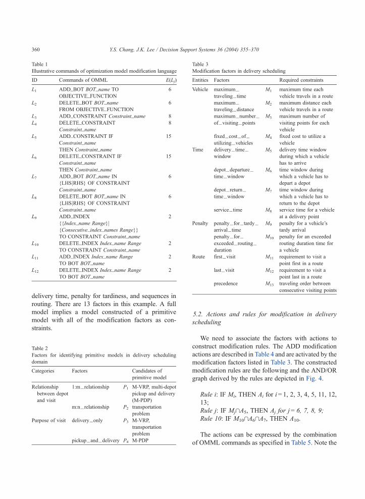
delivery time, penalty for tardiness, and sequences in

routing. There are 13 factors in this example. A full

model implies a model constructed of a primitive

model with all of the modification factors as con-

straints.

5.2. Actions and rules for modification in delivery

scheduling

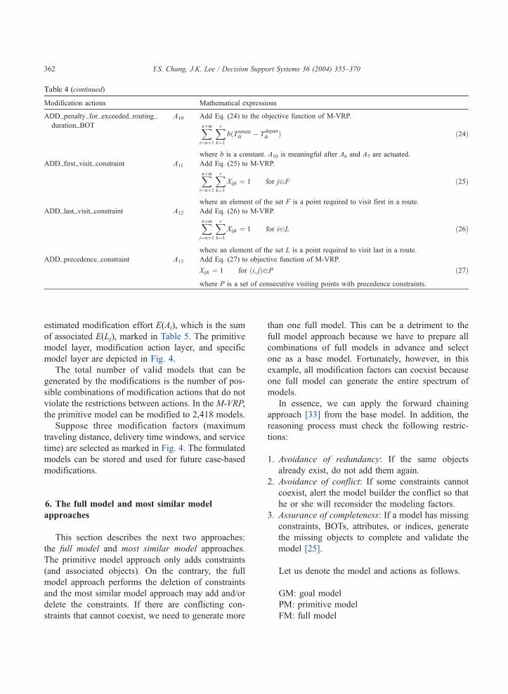
We need to associate the factors with actions to

construct modification rules. The ADD modification

actions are described in Table 4 and are activated by the

modification factors listed in Table 3. The constructed

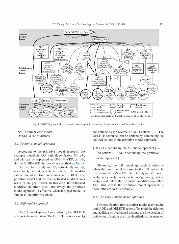
modification rules are the following and the AND/OR

graph derived by the rules are depicted in Fig. 4.

Rule i: IF Mi, THEN Ai for i = 1, 2, 3, 4, 5, 11, 12,

13;

Rule j: IF Mj\A5, THEN Aj for j = 6, 7, 8, 9;

Rule 10: IF M10\A6\A7, THEN A10.

The actions can be expressed by the combination

of OMML commands as specified in Table 5. Note the

Table 2

Factors for identifying primitive models in delivery scheduling

domain

Categories Factors Candidates of

primitive model

Relationship

between depot

and visit

1:m�relationship P1 M-VRP, multi-depot

pickup and delivery

(M-PDP)

m:n�relationship P2 transportation

problem

Purpose of visit delivery�only P3 M-VRP,

transportation

problem

pickup�and�delivery P4 M-PDP

Table 3

Modification factors in delivery scheduling

Entities Factors Required constraints

Vehicle maximum�traveling�time

M1 maximum time each

vehicle travels in a route

maximum�traveling�distance

M2 maximum distance each

vehicle travels in a route

maximum�number�of�visiting�points

M3 maximum number of

visiting points for each

vehicle

fixed�cost�of�utilizing�vehicles

M4 fixed cost to utilize a

vehicle

Time delivery�time�window

M5 delivery time window

during which a vehicle

has to arrive

depot�departure�time�window

M6 time window during

which a vehicle has to

depart a depot

depot�return�time�window

M7 time window during

which a vehicle has to

return to the depot

service�time M8 service time for a vehicle

at a delivery point

Penalty penalty�for�tardy�arrival�time

M9 penalty for a vehicle’s

tardy arrival

penalty�for�exceeded�routing�duration

M10 penalty for an exceeded

routing duration time for

a vehicle

Route first�visit M11 requirement to visit a

point first in a route

last�visit M12 requirement to visit a

point last in a route

precedence M13 traveling order between

consecutive visiting points

Table 1

Illustrative commands of optimization model modification language

ID Commands of OMML E(Lj)

L1 ADD_BOT BOT_name TO

OBJECTIVE_FUNCTION

6

L2 DELETE_BOT BOT_name

FROM OBJECTIVE_FUNCTION

6

L3 ADD_CONSTRAINT Constraint_name 8

L4 DELETE_CONSTRAINT

Constraint_name

8

L5 ADD_CONSTRAINT IF

Constraint_name

THEN Constraint_name

15

L6 DELETE_CONSTRAINT IF

Constraint_name

THEN Constraint_name

15

L7 ADD_BOT BOT_name IN

{LHSjRHS} OF CONSTRAINT

Constraint_name

6

L8 DELETE_BOT BOT_name IN

{LHSjRHS} OF CONSTRAINT

Constraint_name

6

L9 ADD_INDEX

{{Index_name Range}j{Consecutive_index_names Range}}

2

TO CONSTRAINT Constraint_name

L10 DELETE_INDEX Index_name Range

TO CONSTRAINT Constraint_name

2

L11 ADD_INDEX Index_name Range

TO BOT BOT_name

2

L12 DELETE_INDEX Index_name Range

TO BOT BOT_name

2


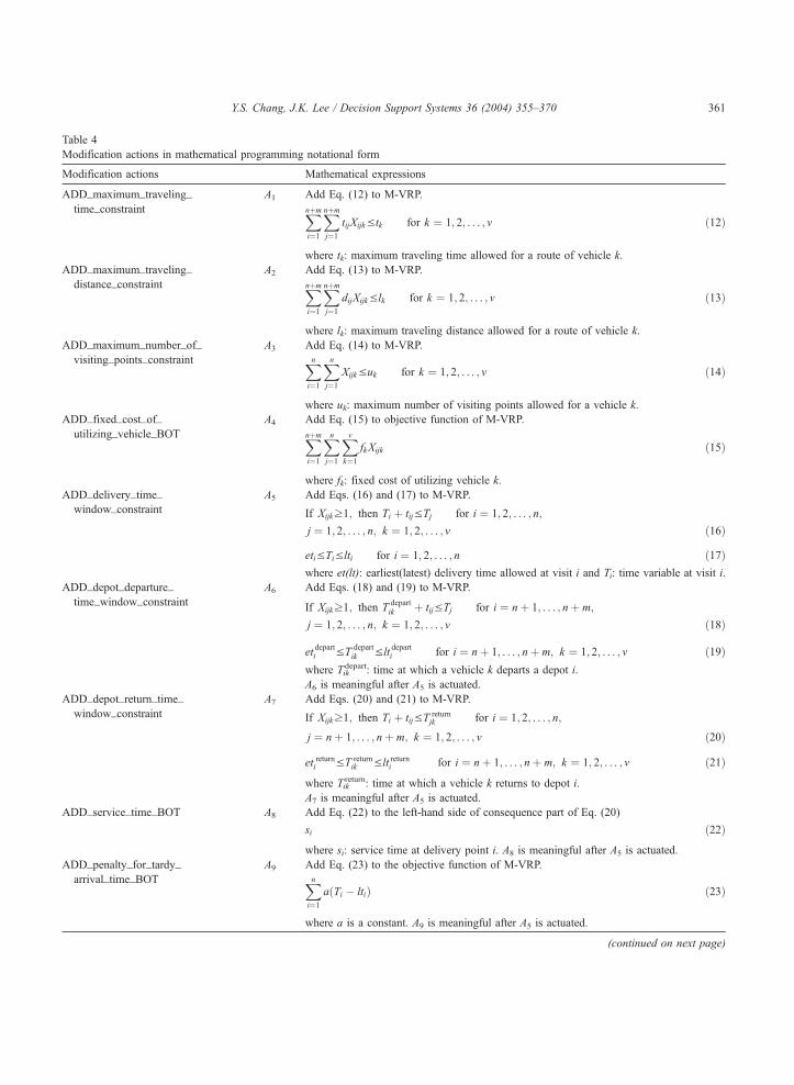
Table 4

Modification actions in mathematical programming notational form

Modification actions Mathematical expressions

ADD_maximum_traveling_ A1 Add Eq. (12) to M-VRP.

time_constraint Xnþm

i¼1

Xnþm

j¼1

tijXijkVtk for k ¼ 1; 2; . . . ; v ð12Þ

where tk: maximum traveling time allowed for a route of vehicle k.

ADD_maximum_traveling_ A2 Add Eq. (13) to M-VRP.

distance_constraint Xnþm

i¼1

Xnþm

j¼1

dijXijkVlk for k ¼ 1; 2; . . . ; v ð13Þ

where lk: maximum traveling distance allowed for a route of vehicle k.

ADD_maximum_number_of_ A3 Add Eq. (14) to M-VRP.

visiting_points_constraint Xn

i¼1

Xn

j¼1

XijkVuk for k ¼ 1; 2; . . . ; v ð14Þ

where uk: maximum number of visiting points allowed for a vehicle k.

ADD_fixed_cost_of_ A4 Add Eq. (15) to objective function of M-VRP.

utilizing_vehicle_BOT Xnþm

i¼1

Xn

j¼1

Xv

k¼1

fkXijk ð15Þ

where fk: fixed cost of utilizing vehicle k.

ADD_delivery_time_ A5 Add Eqs. (16) and (17) to M-VRP.

window_constraint If Xijkz1; then Ti þ tijVTj for i ¼ 1; 2; . . . ; n;

j ¼ 1; 2; . . . ; n; k ¼ 1; 2; . . . ; v ð16Þ

etiVTiVlti for i ¼ 1; 2; . . . ; n ð17Þwhere et(lt): earliest(latest) delivery time allowed at visit i and Ti: time variable at visit i.

ADD_depot_departure_ A6 Add Eqs. (18) and (19) to M-VRP.

time_window_constraintIf Xijkz1; then T

departik þ tijVTj for i ¼ nþ 1; . . . ; nþ m;

j ¼ 1; 2; . . . ; n; k ¼ 1; 2; . . . ; v ð18Þ

etdeparti VT

departik Vlt

departi for i ¼ nþ 1; . . . ; nþ m; k ¼ 1; 2; . . . ; v ð19Þ

where Tikdepart: time at which a vehicle k departs a depot i.

A6 is meaningful after A5 is actuated.

ADD_depot_return_time_ A7 Add Eqs. (20) and (21) to M-VRP.

window_constraint If Xijkz1; then Ti þ tijVT returnjk for i ¼ 1; 2; . . . ; n;

j ¼ nþ 1; . . . ; nþ m; k ¼ 1; 2; . . . ; v ð20Þ

et returni VT returnik Vlt returni for i ¼ nþ 1; . . . ; nþ m; k ¼ 1; 2; . . . ; v ð21Þ

where Tikreturn: time at which a vehicle k returns to depot i.

A7 is meaningful after A5 is actuated.

ADD_service_time_BOT A8 Add Eq. (22) to the left-hand side of consequence part of Eq. (20)

si ð22Þwhere si: service time at delivery point i. A8 is meaningful after A5 is actuated.

ADD_penalty_for_tardy_ A9 Add Eq. (23) to the objective function of M-VRP.

arrival_time_BOT Xn

i¼1

aðTi � ltiÞ ð23Þ

where a is a constant. A9 is meaningful after A5 is actuated.

(continued on next page)


estimated modification effort E(Ai), which is the sum

of associated E(Lj), marked in Table 5. The primitive

model layer, modification action layer, and specific

model layer are depicted in Fig. 4.

The total number of valid models that can be

generated by the modifications is the number of pos-

sible combinations of modification actions that do not

violate the restrictions between actions. In the M-VRP,

the primitive model can be modified to 2,418 models.

Suppose three modification factors (maximum

traveling distance, delivery time windows, and service

time) are selected as marked in Fig. 4. The formulated

models can be stored and used for future case-based

modifications.

6. The full model and most similar model

approaches

This section describes the next two approaches:

the full model and most similar model approaches.

The primitive model approach only adds constraints

(and associated objects). On the contrary, the full

model approach performs the deletion of constraints

and the most similar model approach may add and/or

delete the constraints. If there are conflicting con-

straints that cannot coexist, we need to generate more

than one full model. This can be a detriment to the

full model approach because we have to prepare all

combinations of full models in advance and select

one as a base model. Fortunately, however, in this

example, all modification factors can coexist because

one full model can generate the entire spectrum of

models.

In essence, we can apply the forward chaining

approach [33] from the base model. In addition, the

reasoning process must check the following restric-

tions:

1. Avoidance of redundancy: If the same objects

already exist, do not add them again.

2. Avoidance of conflict: If some constraints cannot

coexist, alert the model builder the conflict so that

he or she will reconsider the modeling factors.

3. Assurance of completeness: If a model has missing

constraints, BOTs, attributes, or indices, generate

the missing objects to complete and validate the

model [25].

Let us denote the model and actions as follows.

GM: goal model

PM: primitive model

FM: full model

Table 4 (continued)

Modification actions Mathematical expressions

ADD_penalty_for_exceeded_routing_ A10 Add Eq. (24) to the objective function of M-VRP.

duration_BOT Xnþm

i¼nþ1

Xv

k¼1

bðT returnik � T

departik Þ ð24Þ

where b is a constant. A10 is meaningful after A6 and A7 are actuated.

ADD_first_visit_constraint A11 Add Eq. (25) to M-VRP.

Xnþm

i¼nþ1

Xv

k¼1

Xijk ¼ 1 for jaF ð25Þ

where an element of the set F is a point required to visit first in a route.

ADD_last_visit_constraint A12 Add Eq. (26) to M-VRP.

Xnþm

j¼nþ1

Xv

k¼1

Xijk ¼ 1 for iaL ð26Þ

where an element of the set L is a point required to visit last in a route.

ADD_precedence_constraint A13 Add Eq. (27) to objective function of M-VRP.

Xijk ¼ 1 for ði; jÞaP ð27Þ

where P is a set of consecutive visiting points with precedence constraints.


SM: a similar case model

A={Ai}: a set of actions

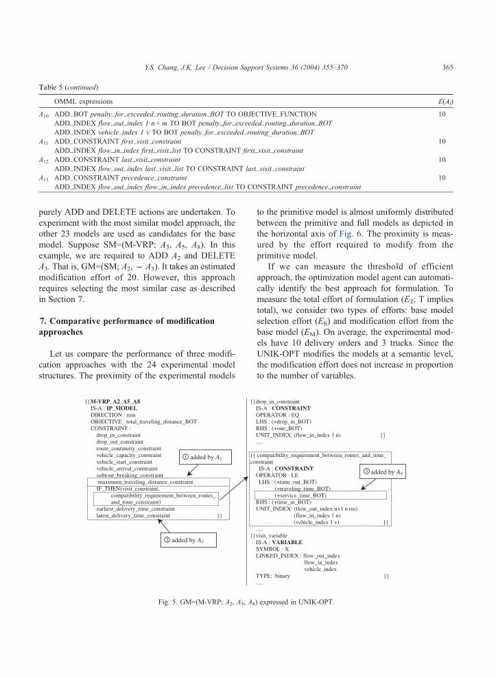
6.1. Primitive model approach

According to the primitive model approach, the

example model M-VRP with three factors M2, M5,

and M8 can be expressed as GM=(M-VRP; A2, A5,

A8). In UNIK-OPT, the model is specified as Fig. 5.

The two factors M2 and M5 activate A2 and A5,

respectively, and M8 and A5 activate A8. The modifi-

cation has added two constraints and a BOT. The

primitive model and the three activated modifications

result in the goal model. In this case, the estimated

modification effort is 63. Intuitively, the primitive

model approach is effective when the goal model is

similar to the primitive model.

6.2. Full model approach

The full model approach must identify the DELETE

actions to be undertaken. The DELETE actions (fAi)

are defined as the reverse of ADD actions (Ai). The

DELETE action set can be derived by eliminating the

ADDed actions in the primitive model approach.

fDELETE actions by the full model approachg ¼fall actionsg � fADD actions by the primitive

model approachg

Obviously, the full model approach is effective

when the goal model is close to the full model. In

this example, GM=(PM; A2, A5, A8)=(FM; fA1,

fA3, fA4, fA6, fA7, fA9, fA10, fA11, fA12,

fA13) and takes the estimated modification effort

182. This means the primitive model approach is

more efficient in this example.

6.3. The most similar model approach

The modification from a similar model may require

both ADD and DELETE actions. To avoid the deletion

and addition of overlapped actions, the intersection of

both types of actions are first identified. In this manner,

Fig. 4. AND/OR graphical relationship between primitive models, factors, actions, and formulated model.


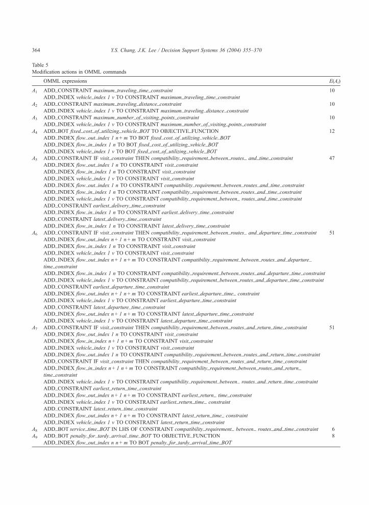
Table 5

Modification actions in OMML commands

OMML expressions E(Ai)

A1 ADD_CONSTRAINT maximum_traveling_time_constraint 10

ADD_INDEX vehicle_index 1 v TO CONSTRAINT maximum_traveling_time_constraint

A2 ADD_CONSTRAINT maximum_traveling_distance_constraint 10

ADD_INDEX vehicle_index 1 v TO CONSTRAINT maximum_traveling_distance_constraint

A3 ADD_CONSTRAINT maximum_number_of_visiting_points_constraint 10

ADD_INDEX vehicle_index 1 v TO CONSTRAINT maximum_number_of_visiting_points_constraint

A4 ADD_BOT fixed_cost_of_utilizing_vehicle_BOT TO OBJECTIVE_FUNCTION 12

ADD_INDEX flow_out_index 1 n+m TO BOT fixed_cost_of_utilizing_vehicle_BOT

ADD_INDEX flow_in_index 1 n TO BOT fixed_cost_of_utilizing_vehicle_BOT

ADD_INDEX vehicle_index 1 v TO BOT fixed_cost_of_utilizing_vehicle_BOT

A5 ADD_CONSTRAINT IF visit_constraint THEN compatibility_requirement_between_routes_ and_time_constraint 47

ADD_INDEX flow_out_index 1 n TO CONSTRAINT visit_constraint

ADD_INDEX flow_in_index 1 n TO CONSTRAINT visit_constraint

ADD_INDEX vehicle_index 1 v TO CONSTRAINT visit_constraint

ADD_INDEX flow_out_index 1 n TO CONSTRAINT compatibility_requirement_between_routes_and_time_constraint

ADD_INDEX flow_in_index 1 n TO CONSTRAINT compatibility_requirement_between_routes_and_time_constraint

ADD_INDEX vehicle_index 1 v TO CONSTRAINT compatibility_requirement_between_ routes_and_time_constraint

ADD_CONSTRAINT earliest_delivery_time_constraint

ADD_INDEX flow_in_index 1 n TO CONSTRAINT earliest_delivery_time_constraint

ADD_CONSTRAINT latest_delivery_time_constraint

ADD_INDEX flow_in_index 1 n TO CONSTRAINT latest_delivery_time_constraint

A6 ADD_CONSTRAINT IF visit_constraint THEN compatibility_requirement_between_routes_ and_departure_time_constraint 51

ADD_INDEX flow_out_index n+ 1 n+m TO CONSTRAINT visit_constraint

ADD_INDEX flow_in_index 1 n TO CONSTRAINT visit_constraint


ADD_INDEX flow_out_index n+ 1 n+m TO CONSTRAINT compatibility_requirement_between_routes_and_departure_

time_constraint

ADD_INDEX flow_in_index 1 n TO CONSTRAINT compatibility_requirement_between_routes_and_departure_time_constraint

ADD_INDEX vehicle_index 1 v TO CONSTRAINT compatibility_requirement_between_routes_and_departure_time_constraint

ADD_CONSTRAINT earliest_departure_time_constraint

ADD_INDEX flow_out_index n+ 1 n+m TO CONSTRAINT earliest_departure_time_ constraint

ADD_INDEX vehicle_index 1 v TO CONSTRAINT earliest_departure_time_constraint

ADD_CONSTRAINT latest_departure_time_constraint

ADD_INDEX flow_out_index n+ 1 n+m TO CONSTRAINT latest_departure_time_constraint

ADD_INDEX vehicle_index 1 v TO CONSTRAINT latest_departure_time_constraint

A7 ADD_CONSTRAINT IF visit_constraint THEN compatibility_requirement_between_routes_and_return_time_constraint 51

ADD_INDEX flow_out_index 1 n TO CONSTRAINT visit_constraint

ADD_INDEX flow_in_index n+ 1 n+m TO CONSTRAINT visit_constraint


ADD_INDEX flow_out_index 1 n TO CONSTRAINT compatibility_requirement_between_routes_and_return_time_constraint

ADD_CONSTRAINT IF visit_constraint THEN compatibility_requirement_between_routes_and_return_time_constraint

ADD_INDEX flow_in_index n+ 1 n+m TO CONSTRAINT compatibility_requirement_between_routes_and_return_

time_constraint

ADD_INDEX vehicle_index 1 v TO CONSTRAINT compatibility_requirement_between_ routes_and_return_time_constraint

ADD_CONSTRAINT earliest_return_time_constraint

ADD_INDEX flow_out_index n+ 1 n+m TO CONSTRAINT earliest_return_ time_constraint

ADD_INDEX vehicle_index 1 v TO CONSTRAINT earliest_return_time_ constraint

ADD_CONSTRAINT latest_return_time_constraint

ADD_INDEX flow_out_index n+ 1 n+m TO CONSTRAINT latest_return_time_ constraint

ADD_INDEX vehicle_index 1 v TO CONSTRAINT latest_return_time_constraint

A8 ADD_BOT service_time_BOT IN LHS OF CONSTRAINT compatibility_requirement_ between_ routes_and_time_constraint 6

A9 ADD_BOT penalty_for_tardy_arrival_time_BOT TO OBJECTIVE_FUNCTION 8

ADD_INDEX flow_out_index n n+m TO BOT penalty_for_tardy_arrival_time_BOT


purely ADD and DELETE actions are undertaken. To

experiment with the most similar model approach, the

other 23 models are used as candidates for the base

model. Suppose SM=(M-VRP; A3, A5, A8). In this

example, we are required to ADD A2 and DELETE

A3. That is, GM=(SM; A2,fA3). It takes an estimated

modification effort of 20. However, this approach

requires selecting the most similar case as described

in Section 7.

7. Comparative performance of modification

approaches

Let us compare the performance of three modifi-

cation approaches with the 24 experimental model

structures. The proximity of the experimental models

to the primitive model is almost uniformly distributed

between the primitive and full models as depicted in

the horizontal axis of Fig. 6. The proximity is meas-

ured by the effort required to modify from the

primitive model.

If we can measure the threshold of efficient

approach, the optimization model agent can automati-

cally identify the best approach for formulation. To

measure the total effort of formulation (ET; T implies

total), we consider two types of efforts: base model

selection effort (ES) and modification effort from the

base model (EM). On average, the experimental mod-

els have 10 delivery orders and 3 trucks. Since the

UNIK-OPT modifies the models at a semantic level,

the modification effort does not increase in proportion

to the number of variables.

OMML expressions E(Ai)

A10 ADD_BOT penalty_for_exceeded_routing_duration_BOT TO OBJECTIVE_FUNCTION 10

ADD_INDEX flow_out_index 1 n+m TO BOT penalty_for_exceeded_routing_duration_BOT

ADD_INDEX vehicle_index 1 v TO BOT penalty_for_exceeded_routing_duration_BOT

A11 ADD_CONSTRAINT first_visit_constraint 10

ADD_INDEX flow_in_index first_visit_list TO CONSTRAINT first_visit_constraint

A12 ADD_CONSTRAINT last_visit_constraint 10

ADD_INDEX flow_out_index last_visit_list TO CONSTRAINT last_visit_constraint

A13 ADD_CONSTRAINT precedence_constraint 10

ADD_INDEX flow_out_index flow_in_index precedence_list TO CONSTRAINT precedence_constraint

Fig. 5. GM=(M-VRP; A2, A5, A8) expressed in UNIK-OPT.

Table 5 (continued)


7.1. Accuracy of the modification effort estimator

The modification effort is estimated by the number

of associated objects as defined in Table 4. To

empirically evaluate the actual effort, we have exe-

cuted the modification and measured the time in

seconds. The estimates and actual execution times

are fitted by a regression model and the resultant

correlation is very high with R2 = 0.992 for the prim-

itive model approach and 0.999 for the full model

approach. Consequently, the estimator is good enough

for the effort prediction.

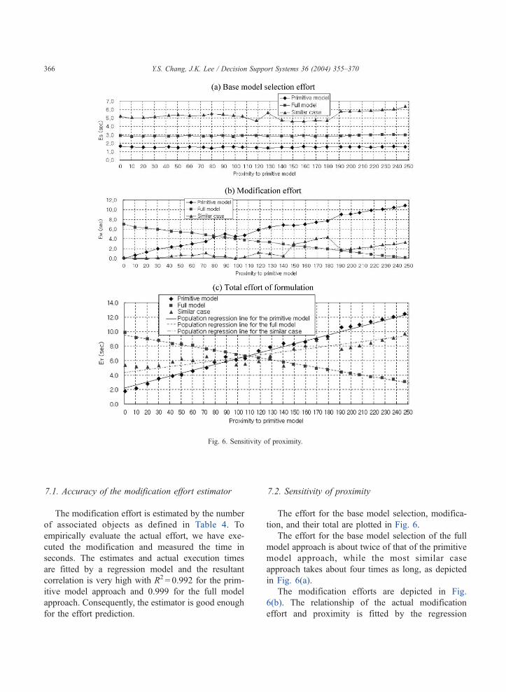
7.2. Sensitivity of proximity

The effort for the base model selection, modifica-

tion, and their total are plotted in Fig. 6.

The effort for the base model selection of the full

model approach is about twice of that of the primitive

model approach, while the most similar case

approach takes about four times as long, as depicted

in Fig. 6(a).

The modification efforts are depicted in Fig.

6(b). The relationship of the actual modification

effort and proximity is fitted by the regression

Fig. 6. Sensitivity of proximity.


model (28). The estimates are summarized in Table

6.

Actual EM ¼ aM þ bM Proximity ð28Þ

The primitive model approach has a positive trend

and the full model approach has a negative trend. The

t-value of the primitive model approach is 53.39 and

that of the full model approach is � 137.71. Thus, the

trends are statistically significant at the 1% level. Note

that the most similar case approach also has a positive

trend, which implies that as the complexity of con-

straints increases, the modification effort even from

the most similar case increases.

The total efforts are depicted in Fig. 6(c). In this

example, the most similar case approach is partially

dominated by the other two approaches at near prox-

imity 100. For the goal models, whose proximity is

less than 107.3, the primitive model approach outper-

forms the most similar case approach. Otherwise, the

full model approach outperforms the others. Accord-

ing to this, the primitive model approach performs best

for the model GM=(M-VRP; A2, A5, A8). The perform-

ance pattern may differ depending upon the applica-

tion domains. We need, therefore, to study the

threshold with experimental data in advance or learn

while using for each application domain. The benefit

increases as the scale of model warehouse expands.

8. Architecture of AGENT-OPT

With the approaches described earlier, we can

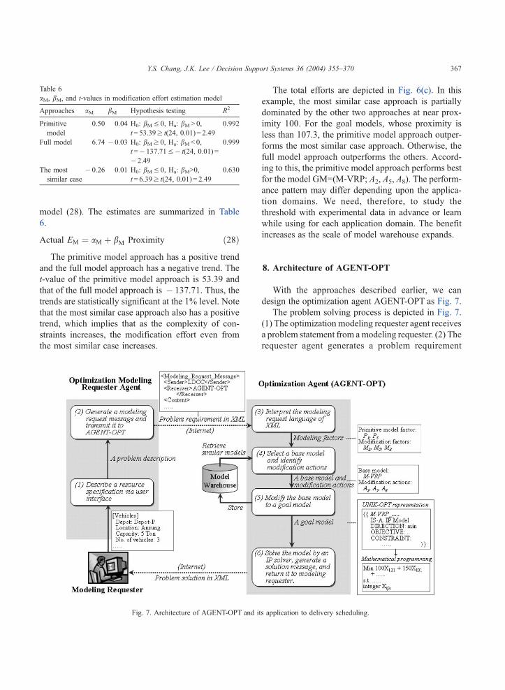
design the optimization agent AGENT-OPT as Fig. 7.

The problem solving process is depicted in Fig. 7.

(1) The optimization modeling requester agent receives

a problem statement from amodeling requester. (2) The

requester agent generates a problem requirement

Table 6

aM, bM, and t-values in modification effort estimation model

Approaches aM bM Hypothesis testing R2

Primitive

model

0.50 0.04 H0: bMV 0, Ha: bM> 0,

t = 53.39z t(24, 0.01) = 2.49

0.992

Full model 6.74 � 0.03 H0: bMz 0, Ha: bM< 0,

t =� 137.71V� t(24, 0.01) =

� 2.49

0.999

The most

similar case

� 0.26 0.01 H0: bMV 0, Ha: bM>0,t = 6.39z t(24, 0.01) = 2.49

0.630

Fig. 7. Architecture of AGENT-OPT and its application to delivery scheduling.


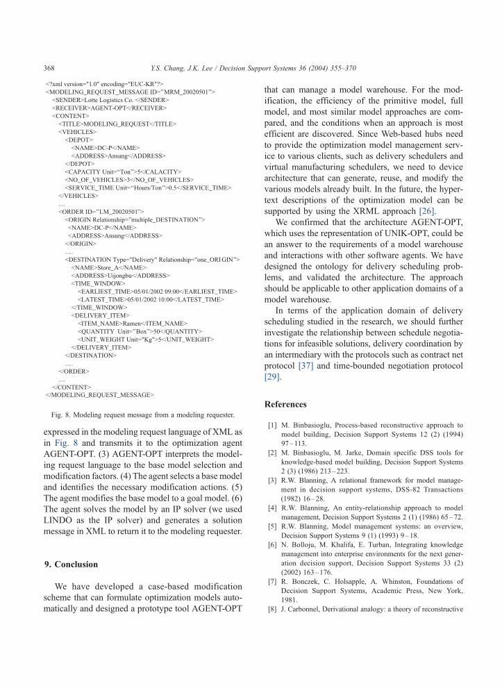
expressed in the modeling request language of XML as

in Fig. 8 and transmits it to the optimization agent

AGENT-OPT. (3) AGENT-OPT interprets the model-

ing request language to the base model selection and

modification factors. (4) The agent selects a base model

and identifies the necessary modification actions. (5)

The agent modifies the base model to a goal model. (6)

The agent solves the model by an IP solver (we used

LINDO as the IP solver) and generates a solution

message in XML to return it to the modeling requester.

9. Conclusion

We have developed a case-based modification

scheme that can formulate optimization models auto-

matically and designed a prototype tool AGENT-OPT

that can manage a model warehouse. For the mod-

ification, the efficiency of the primitive model, full

model, and most similar model approaches are com-

pared, and the conditions when an approach is most

efficient are discovered. Since Web-based hubs need

to provide the optimization model management serv-

ice to various clients, such as delivery schedulers and

virtual manufacturing schedulers, we need to device

architecture that can generate, reuse, and modify the

various models already built. In the future, the hyper-

text descriptions of the optimization model can be

supported by using the XRML approach [26].

We confirmed that the architecture AGENT-OPT,

which uses the representation of UNIK-OPT, could be

an answer to the requirements of a model warehouse

and interactions with other software agents. We have

designed the ontology for delivery scheduling prob-

lems, and validated the architecture. The approach

should be applicable to other application domains of a

model warehouse.

In terms of the application domain of delivery

scheduling studied in the research, we should further

investigate the relationship between schedule negotia-

tions for infeasible solutions, delivery coordination by

an intermediary with the protocols such as contract net

protocol [37] and time-bounded negotiation protocol

[29].

References

[1] M. Binbasioglu, Process-based reconstructive approach to

model building, Decision Support Systems 12 (2) (1994)

97–113.

[2] M. Binbasioglu, M. Jarke, Domain specific DSS tools for

knowledge-based model building, Decision Support Systems

2 (3) (1986) 213–223.

[3] R.W. Blanning, A relational framework for model manage-

ment in decision support systems, DSS-82 Transactions

(1982) 16–28.

[4] R.W. Blanning, An entity-relationship approach to model

management, Decision Support Systems 2 (1) (1986) 65–72.

[5] R.W. Blanning, Model management systems: an overview,

Decision Support Systems 9 (1) (1993) 9–18.

[6] N. Bolloju, M. Khalifa, E. Turban, Integrating knowledge

management into enterprise environments for the next gener-

ation decision support, Decision Support Systems 33 (2)

(2002) 163–176.

[7] R. Bonczek, C. Holsapple, A. Whinston, Foundations of

Decision Support Systems, Academic Press, New York,

1981.

[8] J. Carbonnel, Derivational analogy: a theory of reconstructive

Fig. 8. Modeling request message from a modeling requester.


problem solving and expertise acquisition, in: R. Michalski,

et al. (Eds.), Machine Learning, vol. 2. Morgan Kaufmann,

San Francisco, CA, 1986, pp. 371–392.

[9] D.R. Dolk, B.R. Konsynski, Knowledge representation for

model management systems, IEEE Transactions on Software

Engineering, SE-10:6 (1984) 619–628.

[10] A. Dutta, A. Basu, An artificial intelligence approach to model

management in decision support systems, IEEE Computer 17

(9) (1984) 89–97.

[11] J.J. Elam, J.C. Henderson, L.W. Miller, Model management

systems: an approach to decision support in complex organ-

izations, Proceedings of the First International Conference on

Information System, 1980, pp. 98–110.

[12] A.M. Geoffrion, Introduction to structured modeling, Manage-

ment Science 33 (5) (1987) 547–588.

[13] A.M. Geoffrion, The formal aspects of structured modeling,

Operations Research 37 (1) (1989) 30–51.

[14] S.Y. Huh, Model-base construction with object-oriented con-

structs, Decision Sciences 24 (2) (1993) 409–434.

[15] T. Ishikawa, T. Terano, Analogy by abstraction: case retrieval

and adaptation for inventive design expert systems, Expert

Systems with Applications 10 (3/4) (1996) 351–356.

[16] S.T. Kedar-Cabelli, Toward a Computational Model of Pur-

pose-Directed Analogy, Kaufmann, Analogica, CA, 1988.

[17] C.S. Kim, J.K. Lee, Automatic structural identification and

relaxation for integer programming, Decision Support Sys-

tems 18 (3–4) (1996) 253–271.

[18] B. Konsynski, D.R. Dolk, Knowledge abstractions in model

management, DSS-82 Transactions (1982) 187–202.

[19] R. Krishnan, A logic modeling language for automated model

construction, Decision Support Systems 6 (3) (1990) 123–152.

[20] R.V. Kulkarni, P.R. Bhave, Integer programming formulations

of vehicle routing problems, European Journal of Operational

Research 20 (1985) 58–67.

[21] B. Le Claire, R. Sharda, An Object-oriented Architecture for

Decision Support Systems, 1990 ISDSS Conference Proceed-

ings, 1990, pp. 567–586.

[22] J.S. Lee, Structure frame based model management system,

Unpublished doctoral dissertation, University of Pennsylva-

nia, 1989.

[23] J.S. Lee, A model base for identifying mathematical pro-

gramming structures, Decision Support Systems 7 (2) (1991)

99–105.

[24] J.K. Lee, M.Y. Kim, Knowledge-assisted optimization model

formulation: UNIK-OPT, Decision Support Systems 13 (2)

(1995) 111–132.

[25] J.K. Lee, B.Y. Lee, Integrated management system for opti-

mization and heuristic models, Working paper, KAIST, 2002.

[26] J.K. Lee, M.M. Sohn, eXtensible Rule Markup Language—

Toward the Intelligent Web Platform, Communications of the

ACM, 2002 (forthcoming).

[27] J.K. Lee, Y.U. Song, Unification of linear programming with a

rule-based system by post-model analysis approach, Manage-

ment Science 41 (5) (1995) 835–847.

[28] J.S. Lee, C.V. Jones, M. Guignard, MAPNOS: mathematical

programming formulation normalization system, Expert Sys-

tems With Applications 1 (1990) 367–381.

[29] K.J. Lee, Y.S. Chang, J.K. Lee, Time-bounded negotiation

framework for electronic commerce agents, Decision Support

Systems 28 (4) (2000) 319–331.

[30] M.L. Lenard, An object-oriented approach to model manage-

ment, Decision Support Systems 9 (1) (1993) 67–73.

[31] T.P. Liang, Integrating model management with data manage-

ment in decision support systems, Decision Support Systems 1

(1) (1985) 221–232.

[32] T.P. Liang, Modeling by analogy: a case-based approach to

automated linear program formulation, IEEE, (1991) 276–283.

[33] T.P. Liang, Analogical reasoning and case-based learning in

model management systems, Decision Support Systems 10 (2)

(1993) 137–160.

[34] T.P. Liang, B.R. Konsynski, Modeling by analogy: use of

analogical reasoning in model management systems, Decision

Support Systems 9 (1) (1993) 113–125.

[35] W.A. Muhanna, An object-oriented framework for model

management and DSS development, 1990 ISDSS Conference

Proceedings (1990) 553–565.

[36] S.J. Park, H.D. Kim, Constraint-based metaview approach for

modeling environment generation, Decision Support Systems

9 (4) (1993) 325–348.

[37] R.G. Smith, The contract net protocol: high-level communi-

cation and control in a distributed problem solver, IEEE

Transactions on Computer 29 (1980) 1104–1113.

[38] Y. Tsai, Model integration using SML, Decision Support Sys-

tems 22 (4) (1998) 355–377.

[39] R.C. Vellore, A. Sen, A.S. Vinze, A Case-Based Planning

Approach to Model Formulation, 1990 ISDSS Conference

Proceedings, 1990, pp. 353–382.

[40] W.L. Winston, Operations Research, 3rd ed., Duxbury Press,

Belmont, CA, 1994.

[41] K. Yeom, J.K. Lee, Logical representation of integer program-

ming models, Decision Support Systems 18 (3–4) (1996)

227–251.


Yong Sik Chang has received a PhD

from the Graduate School of Manage-

ment at Korea Advanced Institute of

Science and Technology (KAIST) and

serves as a principal researcher at Inter-

national Center for Electronic Commerce

(ICEC). He received his BS (1988) from

Sogang University and MS (1991) from

Pohang Institute of Science and Technol-

ogy (POSTECH). He has industrial

experiences of developing MIS and elec-

tronic commerce applications. His current research focus is the

electronic commerce, model management, and multi-agent systems.

Jae Kyu Lee is a Professor of Manage-

ment Information Systems at Korea

Advanced Institute of Science and Tech-

nology and a Director of the Interna-

tional Center for Electronic Commerce.

He received a PhD from the Wharton

School, University of Pennsylvania. He

was Chair of the International Confer-

ence on Electronic Commerce (ICEC

1998 and ICEC 2000) and the Third

World Congress on Expert Systems

(1996). He has authored several books on electronic commerce

and expert systems and published numerous papers in the following

journals: Management Science, CACM, DSS, Expert Systems with

Applications, International Journal of Electronic Commerce, Deci-

sion Science, and many others. Currently, he is an Editor-in-Chief of

the Journal Electronic Commerce Research and Applications and

Editorial Member of various international journals like Decision

Support Systems, Expert Systems with Applications, International

Journal of Electronic Commerce, and so on. His main research

interests are in the fields of electronic commerce and intelligent

information systems.


Documents

Case-based modification for optimization agents: AGENT-OPT