PHYSICAL REVIEW E 89, 012808 (2014)

Cavity-based robustness analysis of interdependent networks: Influences of intranetworkand internetwork degree-degree correlations

Shunsuke Watanabe* and Yoshiyuki Kabashima†

Department of Computational Intelligence and Systems Science, Tokyo Institute of Technology, Yokohama 2268502, Japan(Received 6 August 2013; published 16 January 2014)

We develop a methodology for analyzing the percolation phenomena of two mutually coupled (interdependent)networks based on the cavity method of statistical mechanics. In particular, we take into account the influenceof degree-degree correlations inside and between the networks on the network robustness against targeted(random degree-dependent) attacks and random failures. We show that the developed methodology is reducedto the well-known generating function formalism in the absence of degree-degree correlations. The validityof the developed methodology is confirmed by a comparison with the results of numerical experiments. Ouranalytical results indicate that the robustness of the interdependent networks depends on both the intranetworkand internetwork degree-degree correlations in a nontrivial way for both cases of random failures and targetedattacks.

DOI: 10.1103/PhysRevE.89.012808 PACS number(s): 89.75.Hc, 64.60.ah, 89.75.Fb

I. INTRODUCTION

There are many kinds of complex systems in both naturaland artificial worlds, and recently these systems have cometo be studied in various fields by being handled as networks.Networks are expressed mathematically as graphs in which theconstituent elements and interactions among these elementsare expressed as sites (nodes, vertices) and bonds (links,edges), respectively. Random networks in particular [1,2],which are randomly generated networks characterized onlyby their macroscopic properties, have been widely examinedbecause of their analytical tractability.

One major concern surrounding networks is the robustnessagainst random failures (RFs) or targeted attacks (TAs). Thesize of the largest subset of sites that are connected to oneanother, which is often referred to as the giant component(GC) [3], generally becomes smaller as more sites and/orbonds are removed. A standard measure to characterize thenetwork robustness is the critical rate of failure at whichthe fraction of the GC against the size N of the originalnetwork vanishes from O(1) to zero; this is often referredto as the percolation threshold [4,5]. In general, a networkbecomes more tolerant to RFs/TAs as each site in the networkincreases in degree, a parameter that represents the numberof bonds directly connected to the site. On the other hand,increasing the number of bonds is generally costly in termsof various aspects. Therefore, several earlier studies examinedthe robustness of random networks that are specified by onlythe degree distribution while keeping the average degreefixed [6,7]. However, the properties of real-world networkscannot be fully characterized by the degree distribution. As alogical step to take other statistical properties into account,the influences of degree correlations between two directlyconnected sites (degree-degree correlations) were also recentlyexamined [8–10].

More recently, a new type of model that considers inter-dependent networks was proposed [11,12] and has attracted

*watanabe@sp.dis.titech.ac.jp†kaba@dis.titech.ac.jp

significant attention [13–24]. In this model, the system iscomposed of two subnetworks in which the sites in onenetwork are coupled with those in the other on a one-to-onebasis. The two sites of a pair are dependent on each other,so that neither of the sites is functional (active) when eitheris broken (inactive). This interdependence between the twonetworks can facilitate a chain of failures, which is sometimesreferred to as cascade phenomena; removal of sites in onenetwork leads to the emergence of new isolated sites in theother, which then acts as a trigger of new failures in the firstnetwork and the process repeats itself. This mechanism canresult in guidelines for constructing a robust system that aredifferent from those known for single networks. For example,it is known that a broad degree distribution makes a networkmore robust against random site failures in the case of singlenetworks [17], but in interdependent networks, the degrees in anetwork should be uniform to increase the network robustnesswhen the interdependent site pairs are randomly coupledbetween the two networks because sites of a lower degree tendto cause catastrophic breakdowns that amplify the cascadephenomena [11]. In a similar manner to the single-networkcase, the influences of degree-degree correlations in eachnetwork (intranetwork degree-degree correlations) have alsobeen examined numerically [19]. However, as far as the authorsknow, analytical examinations of the intracorrelations andcorrelations between networks (internetwork degree-degreecorrelations) have not yet been reported.

It is against this background that we develop here ananalytical methodology for investigating the influences ofthe intra- and internetwork degree-degree correlations on therobustness of interdependent networks. Our method is basedon the statistical mechanics cavity method developed fordisordered systems [25–27] and evaluates the probability thata pair of interdependent sites characterized by their degreesbelongs to the GC by utilizing the tree approximation underthe assumption that a GC of size O(N ) is formed.

The resultant methodology can be regarded as a gener-alization of the well-known generating function formalism(GFF) [28] that systematically evaluates various topologicalquantities by converting a graph into a transcendental equationof a single variable. One can analytically show that our

1539-3755/2014/89(1)/012808(11) 012808-1 ©2014 American Physical Society

SHUNSUKE WATANABE AND YOSHIYUKI KABASHIMA PHYSICAL REVIEW E 89, 012808 (2014)

methodology is reduced to the GFF in the absence of anydegree correlations; solving a set of nonlinear equations withrespect to multiple variables, which cannot be achieved withthe standard GFF, is indispensable for evaluating the size ofthe GC in the presence of degree-degree correlations.

The remainder of this paper is organized as follows. InSec. II, we briefly summarize the elemental concepts necessaryfor our investigation. In Sec. III, we develop our analyticalmethodology on the basis of the cavity method and discussits relationship with the GFF. In Sec. IV, which is the mainpart of this paper, we demonstrate how the developed method isapplied to interdependent networks, with the results for simpleexamples shown in Sec. V. We end the paper with a summary.

II. PRELIMINARIES ON NETWORKS

We introduce here the definitions of several concepts thatare necessary for our analysis of interdependent networks.We denote the degree distribution by p(k), which indicates thefraction of sites of degree k in a network. Based on this, we candefine the degree distribution of a bond r(k), which representsthe probability that one terminal of a randomly chosen bondhas degree k:

r(k) = kp(k)∑l lp(l)

= kp(k)

〈k〉 , (1)

where 〈k〉 is the average degree when a site in the network ischosen randomly.

Although the degree distribution is a fundamental fea-ture, it is not sufficient to fully characterize the networkproperties [29]. For instance, social networks exhibit theassortative tendency that high-degree sites attach to otherhigh-degree sites. In contrast, technological and biologicalnetworks exhibit the disassortative tendency that high-degreesites preferentially connect with low-degree sites, and viceversa. To introduce such tendencies in a simple manner, wecharacterize our network ensembles by utilizing the jointdegree-degree distribution r(k,l), which is the probability thatthe two terminal sites of a randomly chosen bond have degreesk and l. From this definition, one can relate r(k,l) to p(k) andr(k) as

∑l

r(k,l) = r(k) = kp(k)∑l lp(l)

, (2)

for ∀k.Furthermore, the joint distribution is used to evaluate the

conditional distribution r(k|l), i.e., the probability that oneterminal site of a randomly chosen bond has degree k giventhat the other terminal site has degree l, as

r(k|l) = r(k,l)

r(l)= 〈k〉r(k,l)

lp(l). (3)

When the condition

r(k|l) = r(k) (4)

holds for ∀k,l, the degrees of the directly connected sitesare statistically independent. To macroscopically quantify the

degree-degree correlations, the Pearson coefficient

C = 1

σ 2r

∑kl

kl[r(k,l) − r(k)r(l)], (5)

where

σr =∑

k

k2r(k) −[∑

k

kr(k)

]2

(6)

is often used. If C is zero, then the random network is regardedas uncorrelated. A positive (negative) C indicates assortative(disassortative) mixing.

In a pair of interdependent networks, labeled A and B, weassume that each site in A is coupled with a site in B on aone-to-one basis. We represent the probability that a randomlychosen interdependent pair is composed of a site of degreekA in A and a site of degree kB in B as P (kA,kB). Let usdenote the joint degree-degree distribution for networks A andB as rA(kA,lA) and rB(kB,lB), respectively. For consistency, theidentities

pA(kA) =∑kB

P (kA,kB), (7)

rA(kA) =∑lA

rA(kA,lA) =∑

kBkAP (kA,kB)∑

kA,kBkAP (kA,kB)

, (8)

for network A, and those for network B, must hold. UsingBayes’ formula, the conditional distribution that a site in Ahas degree kA under the condition that the coupled site in Bhas degree kB is evaluated as

PA(kA|kB) = P (kA,kB)∑kB

P (kA,kB), (9)

and

PB(kB|kA) = P (kA,kB)∑kA

P (kA,kB). (10)

Equations (8) and (10) are used for assessing the conditionaldistributions for site pairs; namely, the probability that a sitepair of degrees lA in A and lB in B is connected with anothersite pair of degrees kA in A and kB in B by a link in A, whichis evaluated as

rA(kA,kB|lA,lB) = PB(kB|kA)rA(kA|lA), (11)

and rB(kA,kB|lA,lB) = PA(kA|kB)rB(kB|lB). These conditionaldistributions play an important role in analyzing interdepen-dent networks.

In addition to this statistical characterization, we alsohandle a single realization of randomly generated networks.To specify such a network, we introduce the notation ∂i forthe set of all adjacent sites that are connected directly to sitei and |∂i| for the number of elements in ∂i. We use X\x torepresent a set defined by removing an element x from theset X. Therefore, ∂i\j refers to a set of sites that is definedby removing site j ∈ ∂i from ∂i. For a pair of interdependentnetworks A and B, ∂Ai is used to represent the set of site pairsthat are linked directly to the site pair i in network A, with ∂Bi

being that for network B.We can also represent a network as a bipartite graph. For

this, we denote site i as a circle, an undirected link a between

012808-2

CAVITY-BASED ROBUSTNESS ANALYSIS OF . . . PHYSICAL REVIEW E 89, 012808 (2014)

(a)

(b)

(c)

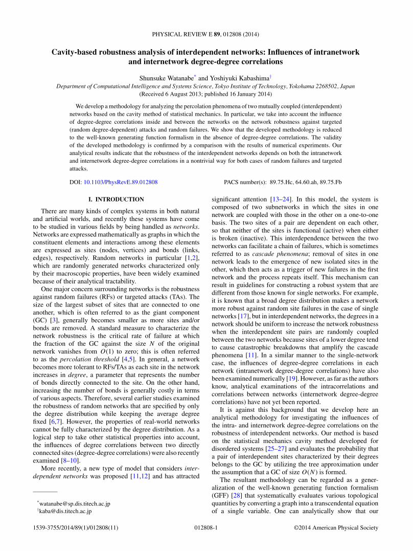
FIG. 1. (a) Graph expression of a network. (b) Bipartite graphexpression of the graph in (a). A square node is assigned for eachedge in (a). (c) Bipartite graph expression of a damaged network.Black square nodes attached to each circle represent whether site i,denoted by the circle, is active (si = 1) or inactive (si = 0).

two sites i and j as a square, and make a link for a related circleand square pair. This generally yields a bipartite graph in whicheach square has two links, while the number of links connectedto a circle varies following a certain degree distribution (Fig. 1).In the bipartite graph expression, we denote ∂a as the set oftwo circles connected to square a and ∂i as the set of squaresconnected to circle i. For a pair of interdependent networks Aand B, ∂Aa and ∂Ai are used to represent the bipartite graphexpression of the connectivity of site pairs in network A, and∂Ba and ∂Bi are used for network B.

III. CAVITY APPROACH TO SINGLE NETWORKS

We review here the cavity approach to the robustnessanalysis of single complex networks, which was developedin an earlier study [8]. The relationship with the GFF [28],another representative technique in research on complexnetworks, is also discussed.

A. Message passing algorithm: Microscopic description

Let us suppose that a network that is sampled from anensemble characterized by p(k) and r(k,l) suffers from RFsor TAs. We employ the binary variable si ∈ {0,1} to representwhether site i is active (si = 1) or inactive (si = 0) due to thefailure. To take the connectivity into account, we introducethe state variable σi ∈ {0,1}, which indicates whether ∃j ∈ ∂i

belongs to the GC (σi = 0) or does not (σi = 1) when i is leftout. Using these definitions, i is regarded as belonging to theGC if and only if si(1 − σi) becomes unity, which gives thesize of the GC as

S = 1

N

N∑i=1

si(1 − σi). (12)

Our analysis is based on the random-network property thatthe lengths of the closed paths between two randomly chosensites (cycles) typically increase as O(ln N ) as the size of thenetwork N tends to infinity, as long as the variance of thedegree distribution is finite. This presumably holds even whenthe degree-degree correlations are introduced and indicatesthat we can locally handle a sufficiently large random networkas a tree.

To incorporate this property in our analysis, we introducethe concept of an i-cavity system, which is defined by removingsite i from the original system. Let us define mj→i = 0 when∃h ∈ ∂j belongs to the GC in the i-cavity system, and mj→i =1, otherwise. Then, σi vanishes if and only if there exists aj ∈ ∂i that is active (sj = 1) and has mj→i = 0. This offersthe basic equation

σi =∏j∈∂i

(1 − sj + sjmj→i). (13)

Given an i-cavity system, we remove a site j ∈ ∂i andswitch i back on instead, which yields a j -cavity system. Then,mi→j vanishes if and only if ∃h ∈ ∂i\j belongs to the GC inthe j -cavity system. A general and distinctive feature of trees isthat when i is removed, ∀j ∈ ∂i are completely disconnectedwith one another. This indicates that mi→j becomes unity ifand only if none of h ∈ ∂i\j belongs to the GC in the i-cavitysystem. These definitions then provide the cavity equation:

mi→j =∏

h∈∂i\j(1 − sh + shmh→i) . (14)

This equation defined for all links over the network determinesthe cavity variables mj→i necessary for evaluating Eq. (13)for every site i. Solving Eq. (14) by the method of iterativesubstitution given the initial condition of mj→i = 0 andsubstituting the obtained solution into Eq. (13) give the size ofthe GC, Eq. (12).

B. Bipartite graph expression

In general, the cavity equations are expressed as messagepassing algorithms on the bipartite graph corresponding toa given network [25]. For this, we denote 1 − sj + sjmj→i

in two ways: Mj→a and Ma→i , where a represents a squareconnected to two circles i and j . Using these, Eqs. (13) and (14)can also be expressed as

Ma→i = Mj→a (∂a = {i,j}), (15)

Mi→a = 1 − si + si

∏b∈∂i\a

Mb→i , (16)

and

σi =∏a∈∂i

Ma→i , (17)

respectively.One advantage of this expression is that the influence

of si can be expressed graphically as an additional squarenode attached to circle i [Fig. 1(c)], which enables us tointerpret Eqs. (15) and (16) as an algorithm that computesan outgoing message along a link from a node on the basis ofincoming messages along the other links to the node. This typeof interpretation is useful for constructing cavity equationsto handle more advanced settings such as interdependentnetworks.

C. Macroscopic description

We turn now to an evaluation of the typical size of theGC when the networks are generated from an ensemble and

012808-3

SHUNSUKE WATANABE AND YOSHIYUKI KABASHIMA PHYSICAL REVIEW E 89, 012808 (2014)

damaged by RFs or TAs. We assume that, as a consequenceof the failures, each site of degree l is active only witha degree-dependent probability ql . We employ the bipartitegraph expression, classify every site by its degree l, anddefine Il to be the frequency that sites of degree l receiveMa→i = 1 among all links of the bipartite graph. Namely,Il is evaluated as Il = (l

∑i δ|∂i|,l)−1 ∑

i(δ|∂i|,l∑

a∈∂i Ma→i),where the denominator is the number of links that connect tosites of degree l, and the numerator is the number of links forwhich Ma→i = 1 is received by sites of degree l.

Although Il has sample-to-sample fluctuations that dependon the network realizations, the strength of the fluctuationstends to zero as N becomes larger. For typical samples, thisindicates that the samples are expected to converge to theiraverage as N → ∞, a property known as self-averaging [25].In the current problem, because of the tree-like property of therandom networks, Il can be evaluated as the expectations withrespect to the graph and failure generations. In the bipartitegraph expression, given a circle of degree l, the conditionaldistribution that the circle is coupled to a circle of degree k

through a square is given by r(k|l). In addition, the probabilitythat the circle of degree k is active is qk . Averaging Eq. (16)with respect to r(k|l) and qk for a fixed value of l and utilizingEq. (15) leads to

Il =∑

k

r(k|l)(1 − qk + qkIk−1k

). (18)

Here, we have employed the property that the average of∏b∈∂i\a Mb→i on the right-hand side of Eq. (16) can be taken

independently of the indices b ∈ ∂i\a because of the treelikenature of random graphs. The whole set in Eq. (18) determinesIl for ∀l. After solving the equations, the typical size of theGC is evaluated as

μ =∑

l

p(l)ql

(1 − I l

l

), (19)

which corresponds to Eq. (12).Equation (18) always allows a trivial solution Il = 1 for ∀l

yielding μ = 0. The local stability of this trivial solution canbe evaluated by linearizing the equations, which gives

δIl =∑

k

(k − 1)qkr(k|l)δIk, (20)

or the alternative expression

δI = AδI, (21)

where A is a matrix defined as

Alk = (k − 1)qkr(k|l). (22)

Equation (21) states that the trivial solution is stable providedμ = 0 if and only if all eigenvalues of A are placed inside theunit circle centered at the origin in the complex plane. As Alk �0 is guaranteed for ∀l and ∀k, the Perron-Frobenius theoremindicates that the critical condition changing this situation isgiven as

det (E − A) = 0, (23)

which determines the percolation threshold for a given set ofcontrol parameters, where E is the identity matrix.

When the active probabilities ql are sufficiently small for∀l, the absolute values of the eigenvalues of A become sosmall that the trivial solution is guaranteed to be stable,yielding a vanishingly small GC size of μ = 0. However, asthe values of ql become larger in a certain manner, Eq. (23) issatisfied at the percolation threshold, and a solution of μ > 0comes continuously from the trivial solution. In this way, theemergence of a large GC is always described as a continuousphase transition for single networks.

D. Connection between the cavity method and generatingfunction formalism

Before proceeding further, we mention briefly the relation-ship between the cavity method and the GFF.

Consider the cases of no degree correlations r(k|l) = r(k)for arbitrary pairs of k,l and no site dependence of the activeprobability ql = q for ∀l. In such cases, Eq. (18) becomesindependent of l, and therefore we can set Il = I . This makesit possible to summarize Eq. (18) as

∑l

r(l)I l−1 =∑

l

r(l)

[1 − q + q

∑k

r(k)I k−1

]l−1

, (24)

which can be expressed more concisely as

f = H (1 − q + qf ), (25)

where we have defined

G(x) =∑

k

p(k)xk, (26)

H (x) =∑

k

r(k)xk−1 = G′(x)

G′(1), (27)

and set f ≡ ∑k r(k)I k−1 = H (I ). Using the solution of

Eq. (25), Eq. (19) is evaluated as

μ = q [1 − G(1 − q + qf )] . (28)

Equation (25) is nothing but a transcendental equationfor the GFF [17]. Namely, the cavity method is reduced tothe GFF in the simplest cases. However, when degree-degreecorrelations exist, Il generally depends on the degree l, andtherefore the cavity equations, Eq. (18), cannot be summarizedas a nonlinear equation of a single variable. As a consequence,one cannot exploit the compact expression of the GFF and hasto directly deal with the cavity equations for evaluating thesize of the GC [8,10]. A similar idea has been implemented inthe GFF by handling a set of coupled generating functions forevaluating the GC of networks free from failures [29].

IV. CAVITY APPROACH FOR INTERDEPENDENTNETWORKS

In this section, we develop the cavity method for analyzingthe cascade phenomena in interdependent networks that occursas a result of RFs or TAs.

A. Cascade phenomena of interdependent networks

Consider the pair of interdependent networks introduced inSec. II. Each pair of sites in networks A and B is interdependent

012808-4

CAVITY-BASED ROBUSTNESS ANALYSIS OF . . . PHYSICAL REVIEW E 89, 012808 (2014)

so that both sites become inactive and lose their functions ifone site becomes inactive. In addition, each active site in Aalso loses its function if it is disconnected from the GC of A,which brings about functional failure of the coupled site inB, and vice versa. In each network, the GC is defined as thelargest subset of functional sites.

We assume initial conditions of all sites being active andfunctional in both networks. In the initial step, sites in A sufferfrom RFs or TAs, and only a portion of the sites remain active.Further, an additional portion of sites lose their functionsbecause they were disconnected from the GC of A. In thesecond step, the sites in B that are coupled with the sites in Athat were disconnected from the GC also lose their functionsdue to the properties of interdependent networks noted above.This reduces the size of the GC in B, and an extra potionof sites in B lose their functions. In the third step, functionalfailure in B is propagated back to A causing further functionalfailure in A, and this process is repeated until convergence.This is the cascade phenomena.

At convergence, every site of the GC in A is coupled witha site of the GC in B on a one-to-one basis. The resultingGC of the site pairs is often termed the mutual GC. Earlierstudies reported that unlike the case of single networks, thesize of the mutual GC relative to the network size vanishesdiscontinuously from O(1) to zero at a critical conditionas the strength of the failures in the initial step becomeslarger [11,12]. We develop here a methodology for examiningthis phenomena on the basis of the cavity method by takingdegree-degree correlations into account.

B. Microscopic description

Let us denote a site pair of the interdependent networks asi. We employ a binary variable si ∈ {0,1} to represent whetheri is kept active in the initial stage (si = 1) or fails (si = 0).We also introduce the state variable σ t

A,i ∈ {0,1} that indicateswhether ∃j ∈ ∂Ai belongs to the GC in A (σ A

i = 0) or doesnot (σ A

i = 1) when i is left out after the t th (t = 1,2, . . .) step,with σB,i being the equivalent state variable for B. Using these,the size of the mutual GC after the 2t th step is expressed as

S2t = 1

N

N∑i=1

si

(1 − σ 2t−1

A,i

)(1 − σ 2t

B,i

). (29)

For a given t , σ 2t−1A,i and σ 2t

B,i can be obtained by the cavitymethod. To do this, we note that the state variables in A afterthe 2t − 1th step can be evaluated by the scheme for single net-works by handing τ 2t−1

A,i = si(1 − σ 2t−2B,i ) as a binary variable

for representing whether i is active (τ 2t−1A,i = 1) or inactive

(τ 2t−1A,i = 0), where σ 0

B,i is set to zero from the assumption.Using the bipartite graph expression (Fig. 2), we get

MAa→i = MA

j→a (∂Aa = {i,j}), (30)

MAi→a = 1 − τ 2t−1

A,i + τ 2t−1A,i

∏b∈∂Ai\a

MAb→i , (31)

and the solution of these yields

σ 2t−1A,i =

∏a∈∂Ai

MAa→i . (32)

A B

(a) (b)

(c)

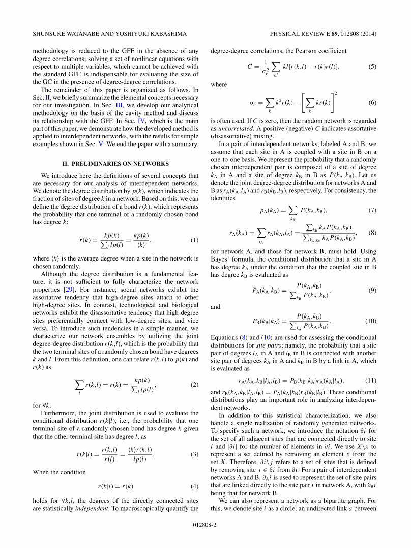
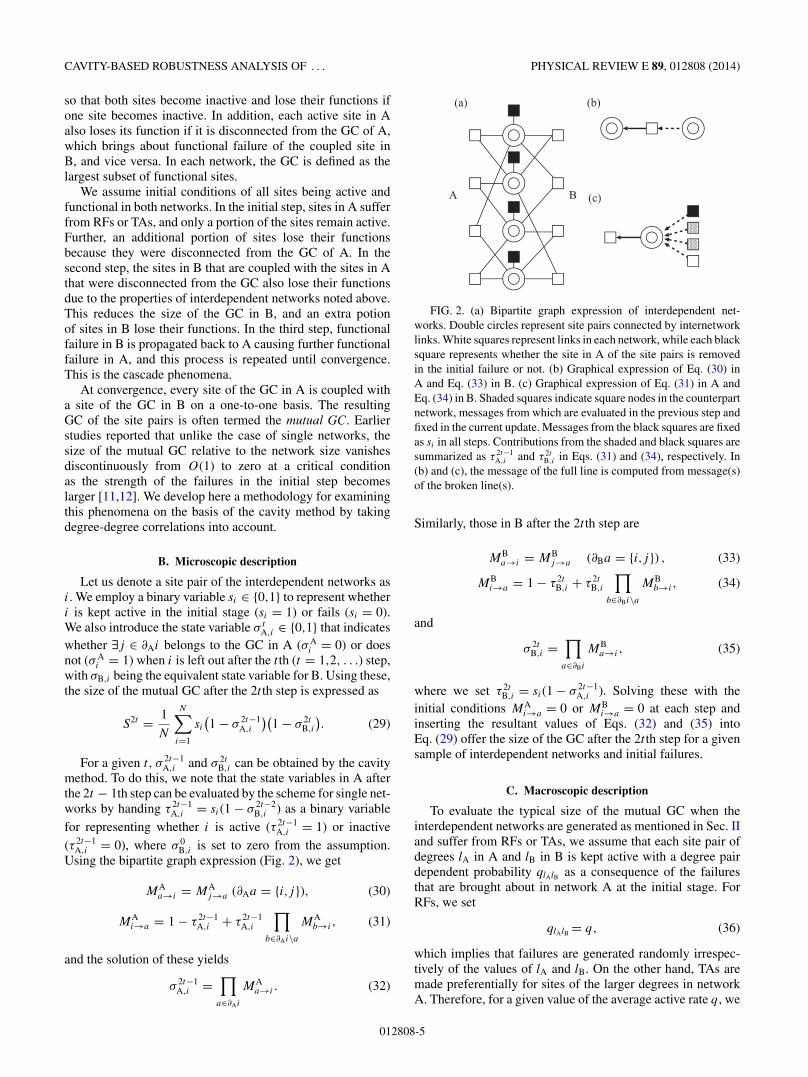
FIG. 2. (a) Bipartite graph expression of interdependent net-works. Double circles represent site pairs connected by internetworklinks. White squares represent links in each network, while each blacksquare represents whether the site in A of the site pairs is removedin the initial failure or not. (b) Graphical expression of Eq. (30) inA and Eq. (33) in B. (c) Graphical expression of Eq. (31) in A andEq. (34) in B. Shaded squares indicate square nodes in the counterpartnetwork, messages from which are evaluated in the previous step andfixed in the current update. Messages from the black squares are fixedas si in all steps. Contributions from the shaded and black squares aresummarized as τ 2t−1

A,i and τ 2tB,i in Eqs. (31) and (34), respectively. In

(b) and (c), the message of the full line is computed from message(s)of the broken line(s).

Similarly, those in B after the 2t th step are

MBa→i = MB

j→a (∂Ba = {i,j}) , (33)

MBi→a = 1 − τ 2t

B,i + τ 2tB,i

∏b∈∂Bi\a

MBb→i , (34)

and

σ 2tB,i =

∏a∈∂Bi

MBa→i , (35)

where we set τ 2tB,i = si(1 − σ 2t−1

A,i ). Solving these with theinitial conditions MA

i→a = 0 or MBi→a = 0 at each step and

inserting the resultant values of Eqs. (32) and (35) intoEq. (29) offer the size of the GC after the 2t th step for a givensample of interdependent networks and initial failures.

C. Macroscopic description

To evaluate the typical size of the mutual GC when theinterdependent networks are generated as mentioned in Sec. IIand suffer from RFs or TAs, we assume that each site pair ofdegrees lA in A and lB in B is kept active with a degree pairdependent probability qlAlB as a consequence of the failuresthat are brought about in network A at the initial stage. ForRFs, we set

qlAlB = q, (36)

which implies that failures are generated randomly irrespec-tively of the values of lA and lB. On the other hand, TAs aremade preferentially for sites of the larger degrees in networkA. Therefore, for a given value of the average active rate q, we

012808-5

SHUNSUKE WATANABE AND YOSHIYUKI KABASHIMA PHYSICAL REVIEW E 89, 012808 (2014)

assign the values of qlAlB as

qlAlB =⎧⎨⎩

0 (lA > �)� (lA = �),1 (lA < �)

(37)

where � and � are uniquely determined so that

q =∑lB

[�P (�,lB) +

∑lA<�

P (lA,lB)

](38)

holds.The key idea of our analysis is basically the same as that

for single networks; namely, we describe the system usingconditional frequencies that a site pair characterized by apair of degrees lA in A and lB in B receives messages ofunity from connected links in A and B. For this, we defineIAlAlB

= (lA∑

i δ|∂Ai|,lAδ|∂Bi|,lB )−1(∑

i δ|∂Ai|,lA∑

a∈∂i MAa→i), and

similarly define IBlAlB

for B.Let us denote q2t−1

A,lAlBas the conditional probability that τ 2t−1

A,i

takes a value of unity for site pairs of degrees lA in A and lBin B at the 2t − 1th step. The self-averaging property and thetree-like nature of random graphs allow us to macroscopicallydescribe Eqs. (30) and (31) as

IAlAlB

=∑kA,kB

rA(kA,kB|lA,lB)

× [1 − q2t−1

A,kAkB+ q2t−1

A,kAkB

(IAkAkB

)kA−1]. (39)

Equation (32) states that the conditional probability of a sitepair of degrees lA in A and lB in B having σ 2t−1

A,i = 1 after the2t − 1th step is (IA

lAlB)lA . Among these sites, only the fraction

of qlAlB is active. Therefore, the conditional probability that asite pair of degrees lA in A and lB in B has τ 2t

B,i = 1 in B at the2t th step is evaluated as

q2tB,lAlB

= qlAlB

[1 − (

IAlAlB

)lA], (40)

using the solution of Eq. (39). Equation (40) makes it possibleto macroscopically describe the cavity equation in B at the2t th step in a similar manner to Eq. (39) as

IBlAlB

=∑kA,kB

rB(kA,kB|lA,lB)

×[1 − q2t

B,kAkB+ q2t

B,kAkB

(IBkAkB

)kB−1]. (41)

Using the solution of Eq. (41), the conditional probability thata site pair of degrees lA in A and lB in B has τ 2t+1

A,i = 1 in A atthe 2t + 1 step is evaluated as

q2t+1A,lAlB

= qlAlB

[1 − (

IBlAlB

)lB]. (42)

Equation (29) gives the expectation of the size of the mutualGC after the 2t th step as

μ2t =∑lA,lB

P (lA,lB)qlAlB

[1 − (

IAlAlB

)lA][

1 − (IBlAlB

)lB]

=∑lA,lB

P (lA,lB)(qlAlB )−1q2t−1A,lAlB

q2tB,lAlB

. (43)

Equations (39)–(43) constitute the main result of the presentpaper.

One thing is noteworthy here. Similar to the case of singlenetworks, Eq. (39) always allows a trivial solution of IA

lAlB= 1,

which becomes stable when sufficiently small q2t−1A,lAlB

valuesare set for all pairs of lA and lB. This yields q2t

B,lAlB= 0 for

all pairs of lA and lB in Eq. (40), which makes IBlAlB

= 1the unique and stable solution of Eq. (41) at the 2t th step,offering μ2t = 0. In addition, at the subsequent 2t + 1th step,q2t+1

A,lAlB= 0 holds for all pairs of lA and lB, which once more

guarantees that the trivial solution is stable. This means thatunlike the case of single networks, the trivial solution ofμ∗ = limt→∞ μ2t = 0 is always locally stable in the dynamicsof Eqs. (39)–(42), irrespective of the strength of the RFs. Afinite μ∗ is obtained when sufficiently large q1

A,lAlB= qlAlB

values are set in the initial step for all pairs of lA and lB.As a consequence, the transition of a finite value of μ∗ to zerogenerally occurs in a discontinuous manner for interdependentnetworks even when degree-degree correlations are taken intoaccount. Earlier studies, however, have already reported theoccurrence of the discontinuous transition for a few specificexamples [11,17,19].

D. Relationship with earlier studies

In Ref. [17], the case involving the highest internetworkdegree-degree correlation [P (kA,kB) = δkB,kAp(kA)] and nointranetwork degree-degree correlation [rA(k,l) = rB(k,l) =r(k)r(l)] is examined for degree-independent RFs character-ized by qlAlB = q. In such a case, we can assume that IA

lAlB=

IBlAlB

= I , ignoring the dependence on the degree and network.Further, we can set limt→∞ q2t−1

A,ll = limt→∞ q2tB,ll = q(1 − I l)

because of the symmetry between networks A and B. Insertingthese into Eq. (39), in conjunction with rA(kA,kB|lA,lB) =δkB,kAr(kA)δlA,lB , we obtain an equation concerning I :

I = 1 − q[1 − IH (I )] + q[H (I ) − IH (I 2)]

= 1 − q[1 − (I + 1)H (I ) + IH (I 2)], (44)

which is equivalent to Eq. (36) in Ref. [17]. The size of themutual GC for t → ∞ is evaluated by inserting IA

lAlB= IB

lAlB=

I into Eq. (43) for P (kA,kB) = δkB,kAp(kA). This provides theexpression

μ∗ = q[1 − 2G(I ) + G(I 2)], (45)

which is also equivalent to Eq. (35) in Ref. [17].In Ref. [11], the case of no intranetwork degree-

degree correlation [rA(k,l) = rA(k)rA(l), rB(k,l) = rB(k)rB(l)]and no internetwork degree-degree correlation [P (kA,kB) =pA(kA)pB(kB)] is discussed. In such a case, one can set IA

lAlB=

IA and IBlAlB

= IB by ignoring the site dependence. Let usfocus on the case of degree-independent RFs qlAlB = q and theconvergent state. Inserting rA(kA,kB|lA,lB) = pB(kB)rA(kA)into Eq. (39) yields

IA = 1 − qB + qB

[∑kA

rA(kA)I kA−1A

]

= 1 − qB + qBfA, (46)

or alternatively

fA = HA(1 − qB + qBfA), (47)

012808-6

CAVITY-BASED ROBUSTNESS ANALYSIS OF . . . PHYSICAL REVIEW E 89, 012808 (2014)

where HA(x) = ∑k rA(k)xk−1 and fA = HA(IA). In a similar

manner, Eq. (41) offers

fB = HB(1 − qA + qAfB), (48)

where HB(x) = ∑k rB(k)xk−1. Equations (42) and (40) pro-

vide qA and qB in Eqs. (47) and (48) in a self-consistent manneras

qA = q

[1 −

∑k

pA(k)I kA

]

= q [1 − GA(1 − qB + qBfA)] (49)

and

qB = q [1 − GB(1 − qA + qAfB)] , (50)

respectively, where GA(x) = ∑k pA(k)xk and GB(x) =∑

k pB(k)xk . Equations (47)–(50) constitute a set of conditionsfor determining four variables: fA,fB,qA, and qB. Using thesevariables, the size of the mutual GC is evaluated as

μ∗ = q [1 − GA(1 − qB + qBfA)]

× [1 − GB(1 − qA + qAfB)] . (51)

For Erdos-Renyi ensembles in particular, which arecharacterized by pA(k) = e−aak/k! and pB(k) = e−bbk/k!,Eqs. (47)–(50) can be summarized as two equations, sinceGA(x) and GB(x) accord to HA(x) and HB(x), respectively,as GA(x) = HA(x) = exp[a(x − 1)] and GB(x) = HB(x) =exp[b(x − 1)]. The resultant coupled equations can be readas

fA = exp [−a(fA − 1)(fB − 1)] (52)

and

fB = exp [−b(fA − 1)(fB − 1)] , (53)

which are identical to Eq. (14) in the Supplemental Materialof Ref. [11].

These two examples show that our scheme can be ex-pressed compactly using the generating functions when themacroscopic cavity variables IA

lAlBand IB

lAlBare independent

of the degrees lA and lB as a consequence of the assumedstatistical features of objective systems and failures. However,correlations of the degrees and/or site dependence of thefailures induces degree dependence of the macroscopic cavityvariables. In such cases, one has no choice but to directlyhandle Eqs. (39)–(43) to theoretically describe the behavior ofinterdependent networks.

V. NUMERICAL TESTS AND RESULTS

A. The flow

To confirm the validity of the analytical scheme, we carriedout numerical experiments using interdependent networks ofN = 10 000 characterized by a set of joint degree distributionsP (kA,kB), rA(kA,lA), and rB(kB,lB) on the basis of the MonteCarlo algorithm proposed in Ref. [29]. We measured the sizeof the GC, using the algorithm proposed in Refs. [30,31].To trigger the cascade phenomena, sites in the constructednetwork A were removed randomly (RF) or preferentially(TA). In each case, we evaluated the size of the mutual GC

after convergence and compared it with the analytical solutionobtained by the cavity method.

As a simple but nontrivial example, we focused on two-peakmodels where the fractions of larger and smaller degrees arefifty-fifty. We set the values of the larger and smaller degreesas 6 and 4, respectively, for both networks A and B. In suchmodels, the intranetwork degree-degree correlations can beuniquely specified by the Pearson coefficient, which is denotedas CA and CB for subnetworks A and B, respectively. However,the influence of the internetwork degree-degree correlationsbetween networks A and B cannot be fully characterizedby only the Pearson coefficient of P (kA,kB), denoted as CI,because pairs of (kA = 4,kB = 6) and (kA = 6,kB = 4) areaffected by the initial removal in different ways for TAs.However, for brevity, we suppose that the fraction of these pairsare the same, which enables us to characterize the intra- andinternetwork degree-degree correlations by three parameters(CA,CB,CI).

The manner in which the failures occur also influences thesize of the mutual GC. In the case of RF, the randomness ofthe initial removal means that the initial survival probabilityof the site pairs does not depend on their degree pairs. Fora TA, however, site pairs that have a higher degree in Aare removed preferentially, and how the removal influencesthe sites in B in the first stage depends on the internetworkdegree-degree correlation. This implies that the robustness ofthe interdependent networks can depend on the internetworkdegree-degree correlations in a nontrivial manner.

B. Results and discussion

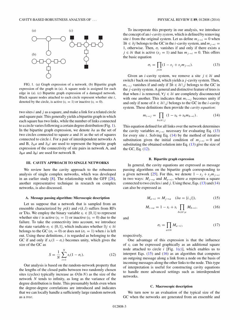
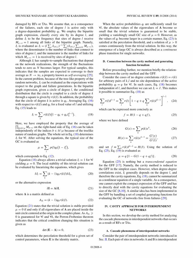
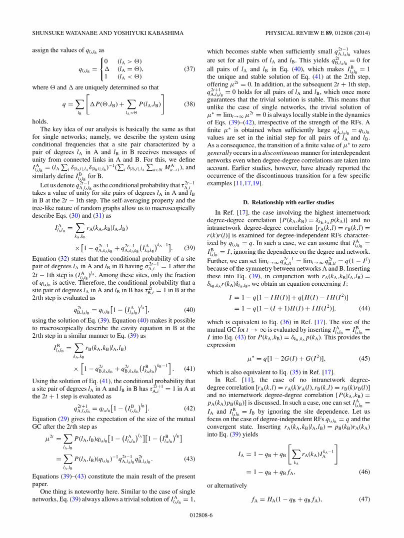
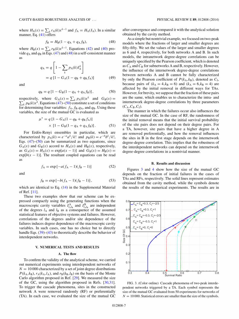
Figures 3 and 4 show how the size of the mutual GCdepends on the fraction of initial failures in the cases ofTAs and RFs, respectively. The solid lines represent estimatesobtained from the cavity method, while the symbols denotethe results of the numerical experiments. The results are in

0.3 0.4 0.5 0.6 0.7 0.80

0.1

0.2

0.3

0.4

0.5

0.6

0.7

0.8

Survival Ratio

Siz

e O

f GC

CA= CB=0.3, CI=−2/3

CA= CB=0.3, CI=1

CA= CB=−0.3, CI=−2/3

CA= CB=−0.3, CI=1

CA= CB=0, CI=0

FIG. 3. (Color online) Cascade phenomena of two-peak interde-pendent networks triggered by a TA. Each symbol represents thesize of the mutual GC evaluated from 50 experiments for networks ofN = 10 000. Statistical errors are smaller than the size of the symbols.

012808-7

SHUNSUKE WATANABE AND YOSHIYUKI KABASHIMA PHYSICAL REVIEW E 89, 012808 (2014)

0.3 0.4 0.5 0.6 0.7 0.80

0.1

0.2

0.3

0.4

0.5

0.6

0.7

0.8

Survival Ratio

Siz

e O

f GC

CA= CB=0.3, CI=−2/3

CA= CB=0.3, CI=1

CA= CB=−0.3, CI=−2/3

CA= CB=−0.3, CI=1

CA= CB=0, CI=0

FIG. 4. (Color online) Cascade phenomena of two-peak interde-pendent networks triggered by a RF. Each symbol represents thesize of the mutual GC evaluated from 50 experiments for networks ofN = 10 000. Statistical errors are smaller than the size of the symbols.

agreement with an excellent accuracy, which validates ourcavity-based analytical scheme. The figures indicate that thepercolation transition of the interdependent networks remainsdiscontinuous irrespective of the introduction of the intra-and/or internetwork degree-degree correlations.

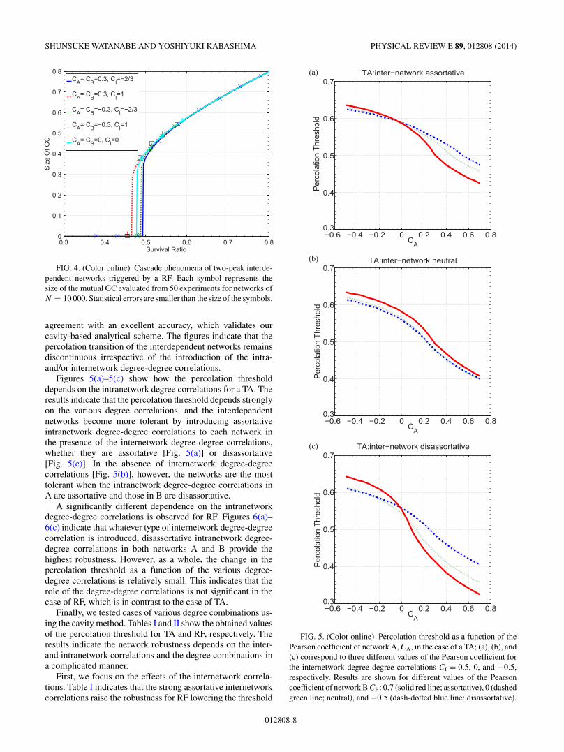
Figures 5(a)–5(c) show how the percolation thresholddepends on the intranetwork degree correlations for a TA. Theresults indicate that the percolation threshold depends stronglyon the various degree correlations, and the interdependentnetworks become more tolerant by introducing assortativeintranetwork degree-degree correlations to each network inthe presence of the internetwork degree-degree correlations,whether they are assortative [Fig. 5(a)] or disassortative[Fig. 5(c)]. In the absence of internetwork degree-degreecorrelations [Fig. 5(b)], however, the networks are the mosttolerant when the intranetwork degree-degree correlations inA are assortative and those in B are disassortative.

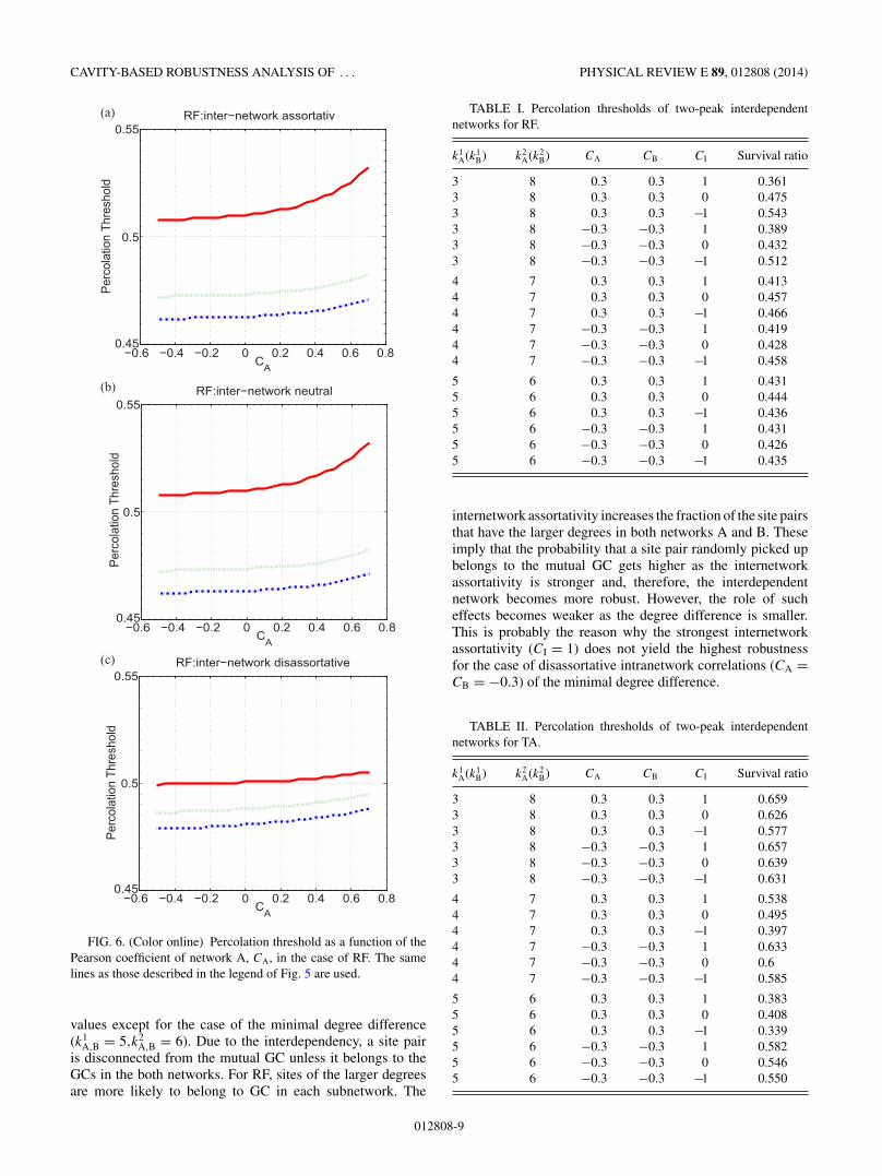
A significantly different dependence on the intranetworkdegree-degree correlations is observed for RF. Figures 6(a)–6(c) indicate that whatever type of internetwork degree-degreecorrelation is introduced, disassortative intranetwork degree-degree correlations in both networks A and B provide thehighest robustness. However, as a whole, the change in thepercolation threshold as a function of the various degree-degree correlations is relatively small. This indicates that therole of the degree-degree correlations is not significant in thecase of RF, which is in contrast to the case of TA.

Finally, we tested cases of various degree combinations us-ing the cavity method. Tables I and II show the obtained valuesof the percolation threshold for TA and RF, respectively. Theresults indicate the network robustness depends on the inter-and intranetwork correlations and the degree combinations ina complicated manner.

First, we focus on the effects of the internetwork correla-tions. Table I indicates that the strong assortative internetworkcorrelations raise the robustness for RF lowering the threshold

(b)

(c)

(a)

−0.6 −0.4 −0.2 0 0.2 0.4 0.6 0.80.3

0.4

0.5

0.6

0.7TA:inter−network assortative

CA

Perc

olat

ion

Thre

shol

d

−0.6 −0.4 −0.2 0 0.2 0.4 0.6 0.80.3

0.4

0.5

0.6

0.7TA:inter−network disassortative

CA

Perc

olat

ion

Thre

shol

d

−0.6 −0.4 −0.2 0 0.2 0.4 0.6 0.80.3

0.4

0.5

0.6

0.7TA:inter−network neutral

CA

Perc

olat

ion

Thre

shol

d

FIG. 5. (Color online) Percolation threshold as a function of thePearson coefficient of network A, CA, in the case of a TA; (a), (b), and(c) correspond to three different values of the Pearson coefficient forthe internetwork degree-degree correlations CI = 0.5, 0, and −0.5,respectively. Results are shown for different values of the Pearsoncoefficient of network B CB: 0.7 (solid red line; assortative), 0 (dashedgreen line; neutral), and −0.5 (dash-dotted blue line: disassortative).

012808-8

CAVITY-BASED ROBUSTNESS ANALYSIS OF . . . PHYSICAL REVIEW E 89, 012808 (2014)

(b)

(c)

−0.6 −0.4 −0.2 0 0.2 0.4 0.6 0.80.45

0.5

0.55RF:inter−network assortativ

CA

Perc

olat

ion

Thre

shol

d

−0.6 −0.4 −0.2 0 0.2 0.4 0.6 0.80.45

0.5

0.55RF:inter−network neutral

CA

Perc

olat

ion

Thre

shol

d

−0.6 −0.4 −0.2 0 0.2 0.4 0.6 0.80.45

0.5

0.55RF:inter−network disassortative

CA

Perc

olat

ion

Thre

shol

d (a)

FIG. 6. (Color online) Percolation threshold as a function of thePearson coefficient of network A, CA, in the case of RF. The samelines as those described in the legend of Fig. 5 are used.

values except for the case of the minimal degree difference(k1

A,B = 5,k2A,B = 6). Due to the interdependency, a site pair

is disconnected from the mutual GC unless it belongs to theGCs in the both networks. For RF, sites of the larger degreesare more likely to belong to GC in each subnetwork. The

TABLE I. Percolation thresholds of two-peak interdependentnetworks for RF.

k1A(k1

B) k2A(k2

B) CA CB CI Survival ratio

3 8 0.3 0.3 1 0.3613 8 0.3 0.3 0 0.4753 8 0.3 0.3 −1 0.5433 8 −0.3 −0.3 1 0.3893 8 −0.3 −0.3 0 0.4323 8 −0.3 −0.3 −1 0.512

4 7 0.3 0.3 1 0.4134 7 0.3 0.3 0 0.4574 7 0.3 0.3 −1 0.4664 7 −0.3 −0.3 1 0.4194 7 −0.3 −0.3 0 0.4284 7 −0.3 −0.3 −1 0.458

5 6 0.3 0.3 1 0.4315 6 0.3 0.3 0 0.4445 6 0.3 0.3 −1 0.4365 6 −0.3 −0.3 1 0.4315 6 −0.3 −0.3 0 0.4265 6 −0.3 −0.3 −1 0.435

internetwork assortativity increases the fraction of the site pairsthat have the larger degrees in both networks A and B. Theseimply that the probability that a site pair randomly picked upbelongs to the mutual GC gets higher as the internetworkassortativity is stronger and, therefore, the interdependentnetwork becomes more robust. However, the role of sucheffects becomes weaker as the degree difference is smaller.This is probably the reason why the strongest internetworkassortativity (CI = 1) does not yield the highest robustnessfor the case of disassortative intranetwork correlations (CA =CB = −0.3) of the minimal degree difference.

TABLE II. Percolation thresholds of two-peak interdependentnetworks for TA.

k1A(k1

B) k2A(k2

B) CA CB CI Survival ratio

3 8 0.3 0.3 1 0.6593 8 0.3 0.3 0 0.6263 8 0.3 0.3 −1 0.5773 8 −0.3 −0.3 1 0.6573 8 −0.3 −0.3 0 0.6393 8 −0.3 −0.3 −1 0.631

4 7 0.3 0.3 1 0.5384 7 0.3 0.3 0 0.4954 7 0.3 0.3 −1 0.3974 7 −0.3 −0.3 1 0.6334 7 −0.3 −0.3 0 0.64 7 −0.3 −0.3 −1 0.585

5 6 0.3 0.3 1 0.3835 6 0.3 0.3 0 0.4085 6 0.3 0.3 −1 0.3395 6 −0.3 −0.3 1 0.5825 6 −0.3 −0.3 0 0.5465 6 −0.3 −0.3 −1 0.550

012808-9

SHUNSUKE WATANABE AND YOSHIYUKI KABASHIMA PHYSICAL REVIEW E 89, 012808 (2014)

The robustness for RFs sometimes leads to the fragilityfor TAs in the case of single networks, e.g., scale-freenetworks [32]. Table II shows that this is also the case as awhole for the interdependent networks. However, the case ofthe minimal degree difference again exhibits an exceptionalbehavior. This is supposed to be due to a similar reason asmentioned for RF.

Next, let us turn to the influences of the intranetworkcorrelations and the degree combinations. Table I indicates thatthe network robustness for RF does not depend significantlyon the intranetwork assortativity (CA = CB) for all degreecombinations, which is consistent with the results suggestedin Fig. 6. On the other hand, Table II shows that therobustness for TA can be influenced largely by the intranetworkassortativity. As a rule of thumb, the stronger intranetworkassortativity is likely to raise the robustness for TA, which,however, does not hold for the case of the large degreedifference (k1

A,B = 3,k2A,B = 8) and the strongest internetwork

assortativity (CI = 1).The results obtained above imply that designing the

most robust interdependent network taking into account thevarious degree-degree correlations is a highly nontrivial andchallenging task.

VI. SUMMARY

In summary, we have developed an analytical methodologyfor evaluating the size of the mutual GC for basic interde-pendent networks composed of two subnetworks A and B.The methodology is based on the cavity method, which makesit possible to evaluate the size of the GC against TAs andRFs by solving a set of macroscopic nonlinear equations

derived from a local tree approximation in conjunction withthe self-averaging property. We have shown that the cavity-based methodology is reduced to the widely known GFF inthe absence of any degree correlations and that solving thefull-cavity equations is indispensable for evaluating the size ofthe GC in the presence of degree-degree correlations.

We compared the estimates of the size of the mutual GCwith the results of numerical experiments on two-peak degreedistribution models for site removal processes of TAs andRFs; there was excellent consistency between the theory andexperiments, which validated the developed methodology. Theutility of the methodology was demonstrated by analyzing thedegree correlation dependence of the percolation threshold,which indicated that the network robustness for TAs is sensitiveto the intra- and internetwork degree-degree correlations,whereas the significance of the degree-degree correlations isrelatively small for RFs.

Promising directions for future work include exploring themost robust structure of an interdependent network system andmore general models that exemplify real-world systems.

ACKNOWLEDGMENTS

The authors thank Koujin Takeda for useful comments anddiscussions. The authors also appreciate anonymous refereeswhose remarks contribute greatly to the final version of thepaper. This work was partially supported by JSPS/MEXTKAKENHI Grants No. 22300003, No. 22300098, and No.25120013 (Y.K.). Encouragement from the ELC project(Grant-in-Aid for Scientific Research on Innovative Areas,JSPS/MEXT, Japan) is also acknowledged.

[1] P. Erdos and A. Reyni, Publ. Math. 6, 290 (1959).[2] B. Bollobas, S. Janson, and O. Riordan, Random Struct. Alg.

31, 3 (2007).[3] S. Janson, D. E. Knuth, T. Łuczak, and B. Pittel, Random Struct.

Alg. 4, 233 (1993).[4] S. Kirkpatrick, Rev. Mod. Phys. 45, 574 (1973).[5] D. S. Callaway, M. E. J. Newman, S. H. Strogatz, and D. J.

Watts, Phys. Rev. Lett. 85, 5468 (2000).[6] A. X. C. N. Valente, A. Sarkar, and H. A. Stone, Phys. Rev. Lett.

92, 118702 (2004).[7] G. Paul, T. Tanizawa, S. Havlin, and H. E. Stanley, Eur. Phys. J.

B 38, 187 (2004).[8] Y. Shiraki and Y. Kabashima, Phys. Rev. E 82, 036101 (2010).[9] E. Agliari, C. Cioli, and E. Guadagnini, Phys. Rev. E 84, 031120

(2011).[10] T. Tanizawa, S. Havlin, and H. E. Stanley, Phys. Rev. E 85,

046109 (2012).[11] S. V. Buldyrev, R. Parshani, G. Paul, H. E. Stanley, and

S. Havlin, Nature 464, 1025 (2010).[12] R. Parshani, S. V. Buldyrev, and S. Havlin, Phys. Rev. Lett. 105,

048701 (2010).[13] J. Gao, S. V. Buldyrev, S. Havlin, and H. E. Stanley, Phys. Rev.

Lett. 107, 195701 (2011).

[14] S. W. Son, P. Grassberger, and M. Paczuski, Phys. Rev. Lett.107, 195702 (2011).

[15] R. G. Morris and M. Barthelemy, Phys. Lett. 109, 128703(2012).

[16] G. J. Baxter, S. N. Dorogovtsev, A. V. Goltsev, and J. F. F.Mendes, Phys. Lett. 109, 248701 (2012).

[17] S. V. Buldyrev, N. W. Shere, and G. A. Cwilich, Phys. Rev. E83, 016112 (2011).

[18] R. R. Liu, W. X. Wang, Y. C. Lai, and B. H. Wang, Phys. Rev.E 85, 026110 (2012).

[19] D. Zhou, H. E. Stanley, G. D’Agostino, and A. Scala, Phys. Rev.E 86, 066103 (2012).

[20] C. M. Schneider, N. A. M. Araujo, and H. J. Herrmann, Phys.Rev. E 87, 043302 (2013).

[21] R. Parshani, C. Rozenblat, D. Ietri, C. Ducruet, and S. Havlin,Europhys. Lett. 92, 68002 (2010).

[22] Z. Wang, A. Szolnoki, and M. Perc, Europhys. Lett. 97, 48001(2012).

[23] B. Min, S. D. Yi, K.-M. Lee, and K.-I. Goh, arXiv:1307.1253.[24] D. Cellai, E. Lopez, J. Zhou, J. P. Gleeson, and G. Bianconi,

arXiv:1307.6359.[25] M. Mezard, G. Parsi, and M. Virasoro, Spin Glass Theory and

Beyond (World Scientific, Singapore, 1987).

012808-10

CAVITY-BASED ROBUSTNESS ANALYSIS OF . . . PHYSICAL REVIEW E 89, 012808 (2014)

[26] M. Mezard and G. Parsi, Eur. Phys. J. B 20, 217 (2001).[27] M. Mezard and Montanari, Information, Physics, and

Computation (Oxford University Press, Oxford, 2009).[28] M. E. J. Newman, S. H. Strogatz, and D. J. Watts, Phys. Rev. E

64, 026118 (2001).

[29] M. E. J. Newman, Phys. Rev. Lett. 89, 208701 (2002).[30] J. Hoshen and R. Kopelman, Phys. Rev. B 14, 3438 (1976).[31] A. Al-Futaisi and T. W. Patzek, Physica A 321, 665 (2003).[32] R. Albert and A.-L. Barabasi, Rev. Mod. Phys. 74, 47

(2002).

012808-11