Contents

1. What is an Image sensor

2. CCD Image Sensors

3. CMOS Image Sensors

4. Main Advantages/Disadvantages between CMOS and CCD

5. Matlab Image processing toolbox

What is an Image Sensor?

An Image Sensor is a photosensitive device that converts light signals into digital signals (colours/RGB data).

Typically, the two main types in common use are CCD and CMOS sensors and are mainly used in digital cameras and other imaging devices.

CCD stands for Charged-Coupled Device and CMOS stands for Complementary Metal–Oxide–Semiconductor

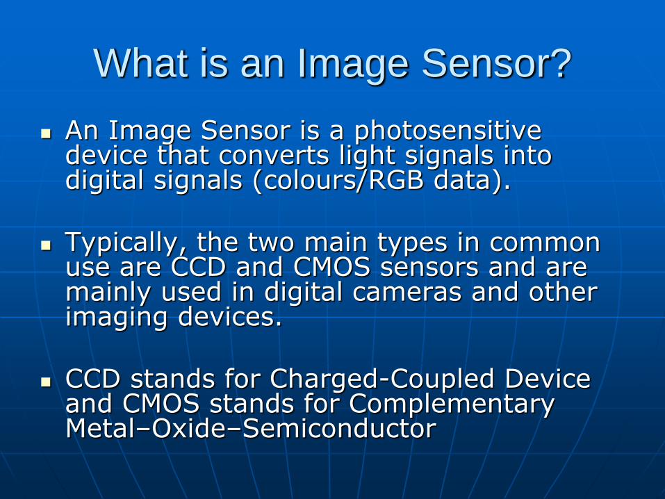
Uses: imaging-spectroscopy

Image sensors are not only limited to digital cameras.

Image sensors are used in other fields such as:

• Machine vision/sensing

• UV Spectroscopy

• Etc.

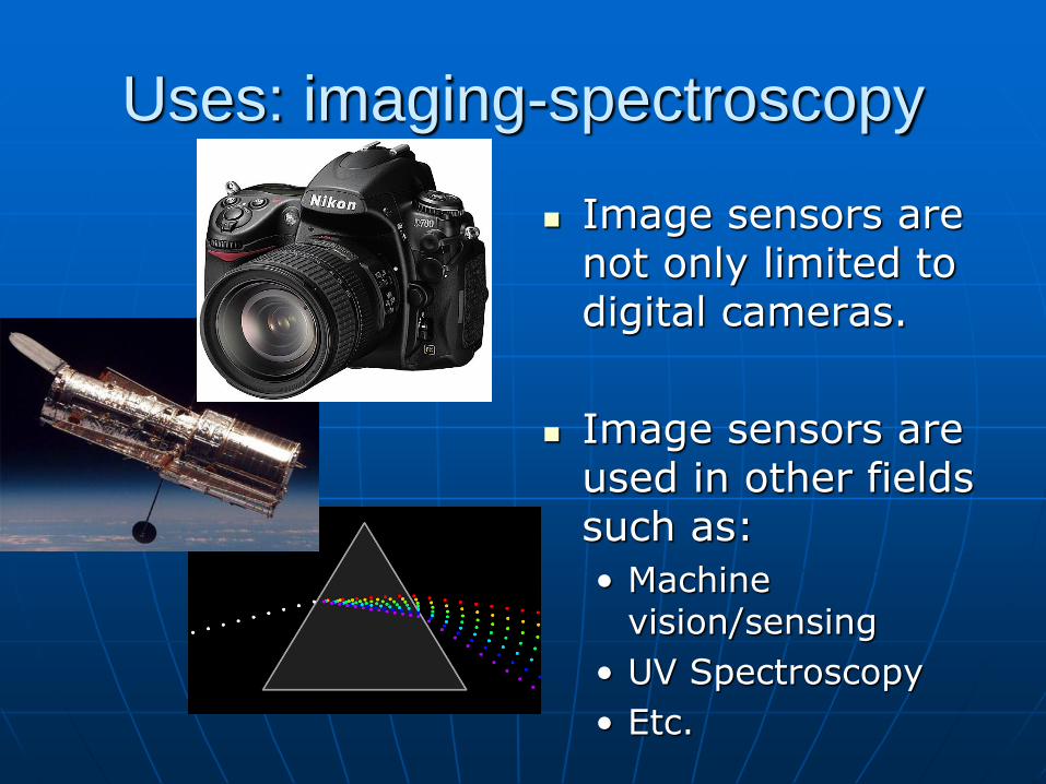
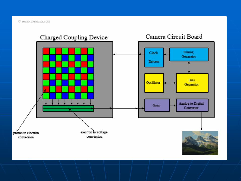
How CCDs Record Colour Each CCD cell in the CCD array

produces a single value independent of colour.

To make colour images, CCD cells are organized in groups of four cells (making one pixel) and a Bayer Filter is placed on top of the group to allow only red light to hit one of the four cells, blue light to hit another and green light to hit the remaining two.

The reasoning behind the two green cells is because the human eye is more sensitive to green light and it is more convenient to use a 4 pixel filter than a 3 pixel filter (harder to implement) and can be compensated after a image capture with something called white balance.

Ex. A Bayer filter applied to the underlying CCD pixel

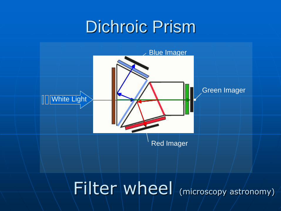
Dichroic Prism

White Light

Blue Imager

Green Imager

Red Imager

Filter wheel (microscopy astronomy)

CCD

A CCD, or a Charged-Coupled Device, is a photosensitive analog device that records light as a small electrical charge in each of its pixels or cells. In essence a CCD is an collection of CCD cells.

The signal captured by the CCD requires additional

circuitry to convert the analog light data into a readable digital signal.

This is mainly layers of capacitors called Stages

which act as a way to transport the analog signal to an array of flip-flops which store the data all controlled by a clock signal.

This is the definition of an Analog Shift Register.

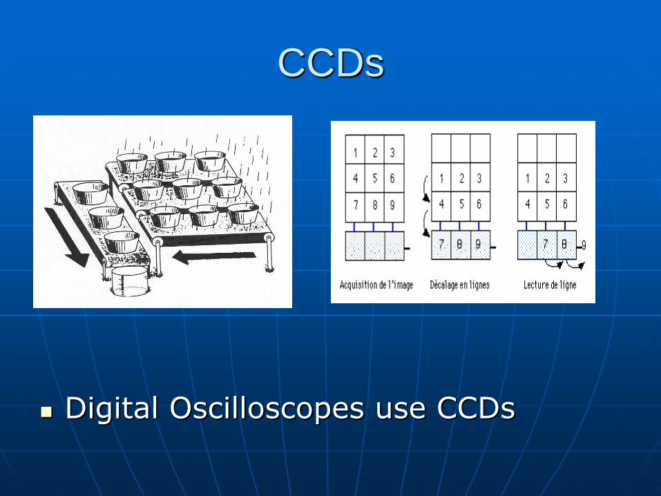
CCDs

Digital Oscilloscopes use CCDs

CMOS

A CMOS, or Complementary Metal Oxide Semiconductor, each pixel has neighboring transistors which locally perform the analog to digital conversion.

This difference in readout has many implications in the overall organization and capability of the camera.

Each one of these pixel sensors are called an Active Pixel Sensor (APS).

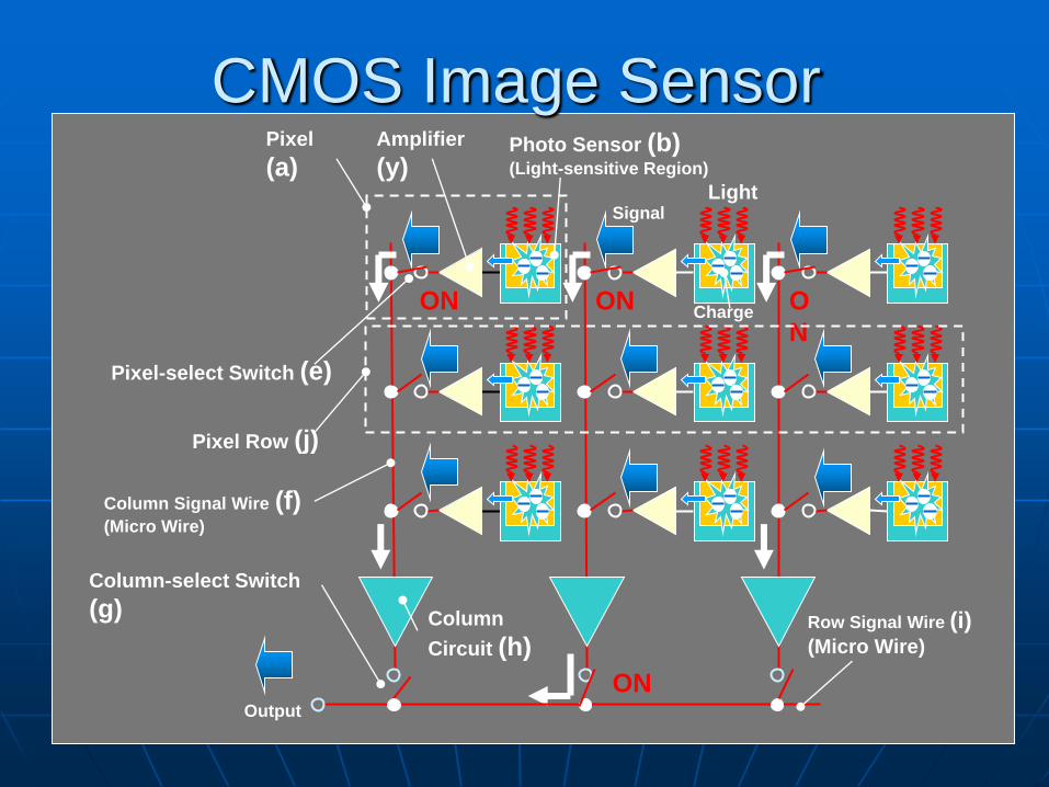
Photo Sensor (b) (Light-sensitive Region)

Light

Charge

Signal

Amplifier

(y) Pixel

(a)

Column Signal Wire (f) (Micro Wire)

Pixel-select Switch (e)

ON ON O

N

Output

ON

Column

Circuit (h) Row Signal Wire (i) (Micro Wire)

Column-select Switch

(g)

Pixel Row (j)

CMOS Image Sensor

CMOS

The imaging logic is integrated on a CMOS chip, where a CCD is a modular imager that can be replaced.

Because of this, design of a new CMOS chip is more expensive.

However, APSs are transistor-based, which means that CMOS chips can be cheaply manufactured on any standard silicon production line.

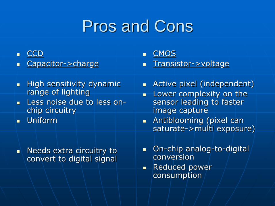
Pros and Cons

CCD

Capacitor->charge

High sensitivity dynamic range of lighting

Less noise due to less on-chip circuitry

Uniform

Needs extra circuitry to convert to digital signal

CMOS

Transistor->voltage

Active pixel (independent)

Lower complexity on the sensor leading to faster image capture

Antiblooming (pixel can saturate->multi exposure)

On-chip analog-to-digital conversion

Reduced power consumption

What is the Image Processing Toolbox?

• The Image Processing Toolbox is a collection of

functions that extend the capabilities of the MATLAB’s

numeric computing environment. The toolbox supports a

wide range of image processing operations, including:

– Geometric operations

– Neighborhood and block operations

– Linear filtering and filter design

– Transforms

– Image analysis and enhancement

– Binary image operations

– Region of interest operations

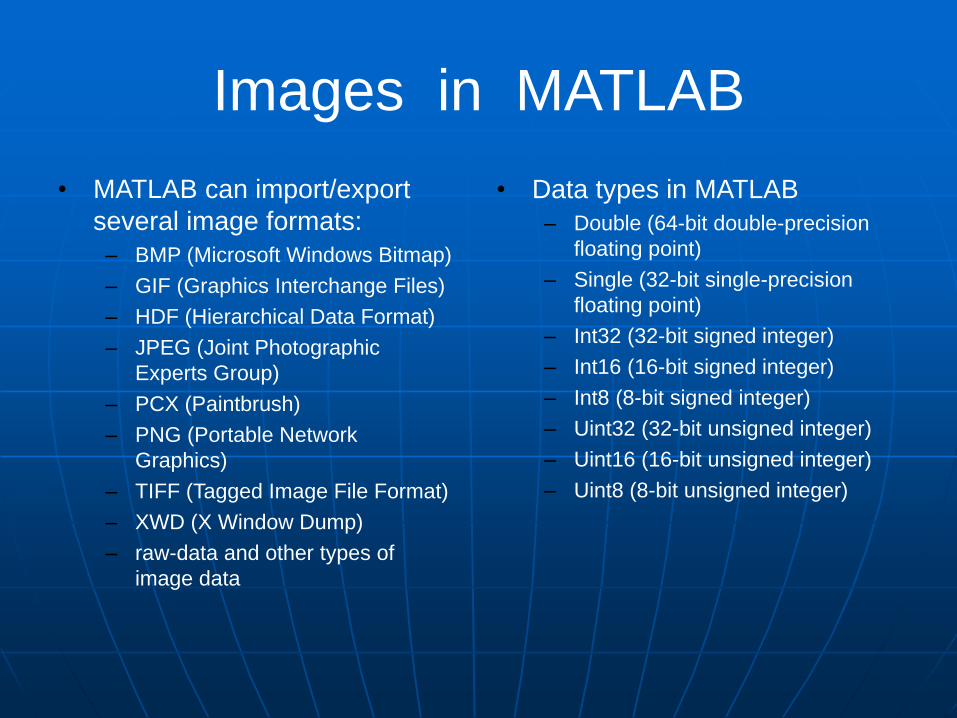
Images in MATLAB

• MATLAB can import/export

several image formats:

– BMP (Microsoft Windows Bitmap)

– GIF (Graphics Interchange Files)

– HDF (Hierarchical Data Format)

– JPEG (Joint Photographic

Experts Group)

– PCX (Paintbrush)

– PNG (Portable Network

Graphics)

– TIFF (Tagged Image File Format)

– XWD (X Window Dump)

– raw-data and other types of

image data

• Data types in MATLAB

– Double (64-bit double-precision

floating point)

– Single (32-bit single-precision

floating point)

– Int32 (32-bit signed integer)

– Int16 (16-bit signed integer)

– Int8 (8-bit signed integer)

– Uint32 (32-bit unsigned integer)

– Uint16 (16-bit unsigned integer)

– Uint8 (8-bit unsigned integer)

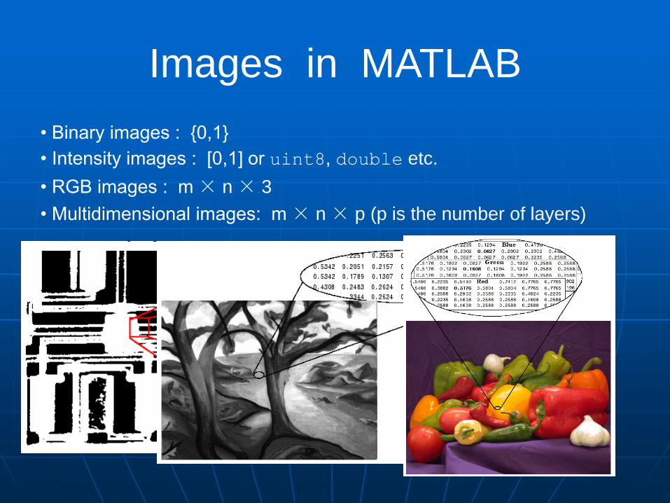
Images in MATLAB

• Binary images : {0,1}

• Intensity images : [0,1] or uint8, double etc.

• RGB images : m × n × 3

• Multidimensional images: m × n × p (p is the number of layers)

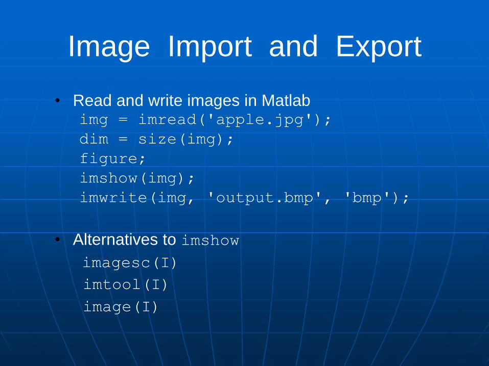
Image Import and Export

• Read and write images in Matlab img = imread('apple.jpg');

dim = size(img);

figure;

imshow(img);

imwrite(img, 'output.bmp', 'bmp');

• Alternatives to imshow

imagesc(I)

imtool(I)

image(I)

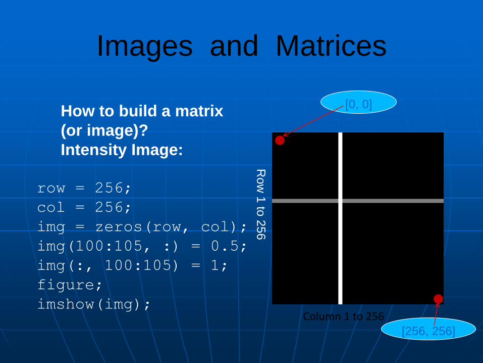
Images and Matrices

Column 1 to 256

Row

1 to

256

o

[0, 0]

o

[256, 256]

How to build a matrix

(or image)?

Intensity Image:

row = 256;

col = 256;

img = zeros(row, col);

img(100:105, :) = 0.5;

img(:, 100:105) = 1;

figure;

imshow(img);

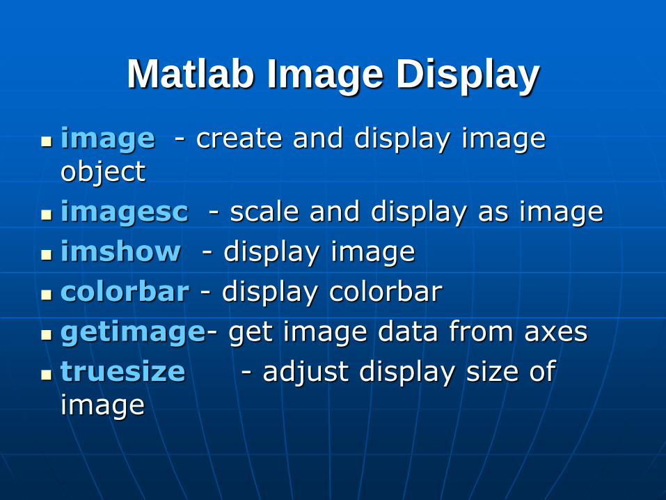
Matlab Image Display

image - create and display image object

imagesc - scale and display as image

imshow - display image

colorbar - display colorbar

getimage- get image data from axes

truesize - adjust display size of image

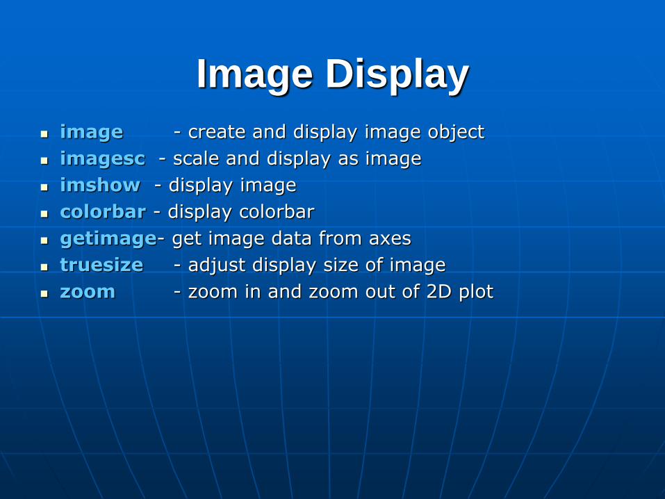
Image Display

image - create and display image object

imagesc - scale and display as image

imshow - display image

colorbar - display colorbar

getimage- get image data from axes

truesize - adjust display size of image

zoom - zoom in and zoom out of 2D plot

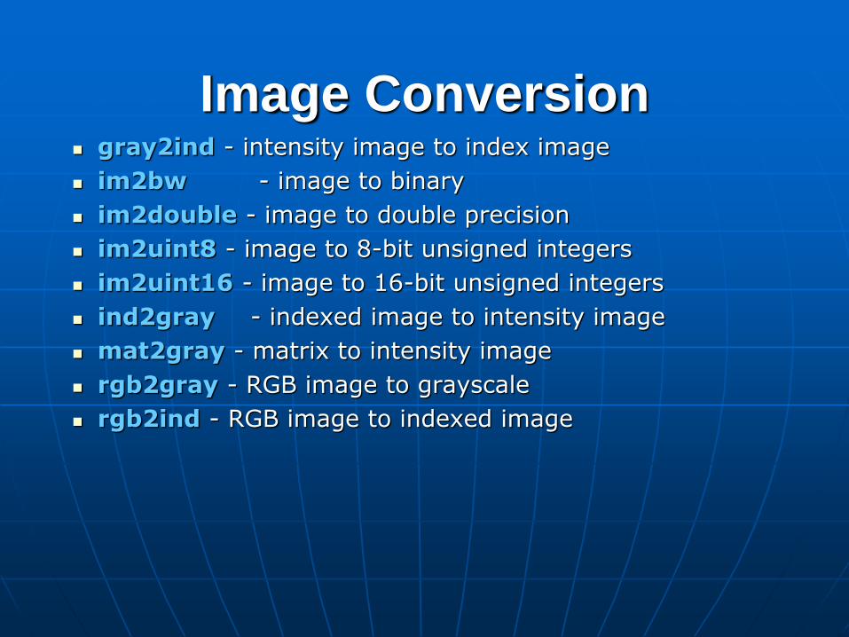
Image Conversion gray2ind - intensity image to index image

im2bw - image to binary

im2double - image to double precision

im2uint8 - image to 8-bit unsigned integers

im2uint16 - image to 16-bit unsigned integers

ind2gray - indexed image to intensity image

mat2gray - matrix to intensity image

rgb2gray - RGB image to grayscale

rgb2ind - RGB image to indexed image

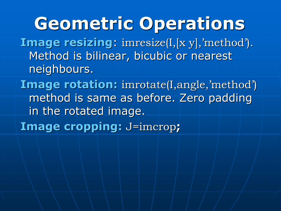
Geometric Operations Image resizing: imresize(I,[x y],’method’).

Method is bilinear, bicubic or nearest neighbours.

Image rotation: imrotate(I,angle,’method’)

method is same as before. Zero padding in the rotated image.

Image cropping: J=imcrop;

23

Neighbourhood Processing

To speed up neighbourhood processing transform every neighbourhood to column vector and perform vector operations.

The borders are usually padded with zeros for the computations of the edges neighborhoods.

Linear filtering can be done with convolution

- conv2(Img, h) or correlation

- filter2(Img, h).

Nonlinear filtering: nlfilter(I,[sx sy],’func’) where func is a

function that receives the windows and returns scalars.

24

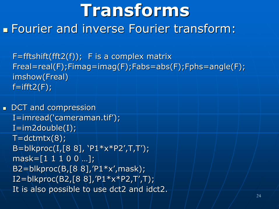
Transforms Fourier and inverse Fourier transform:

F=fftshift(fft2(f)); F is a complex matrix

Freal=real(F);Fimag=imag(F);Fabs=abs(F);Fphs=angle(F);

imshow(Freal)

f=ifft2(F);

DCT and compression

I=imread(‘cameraman.tif’);

I=im2double(I);

T=dctmtx(8);

B=blkproc(I,[8 8], ‘P1*x*P2’,T,T’);

mask=[1 1 1 0 0 …];

B2=blkproc(B,[8 8],’P1*x’,mask);

I2=blkproc(B2,[8 8],’P1*x*P2,T’,T);

It is also possible to use dct2 and idct2.

25

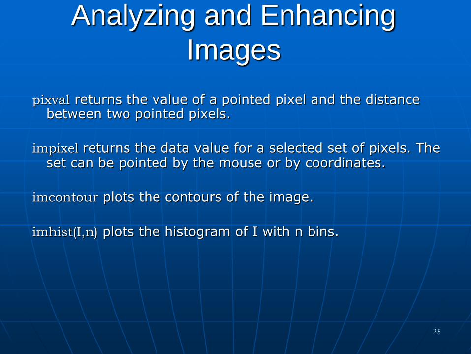
Analyzing and Enhancing

Images

pixval returns the value of a pointed pixel and the distance between two pointed pixels.

impixel returns the data value for a selected set of pixels. The set can be pointed by the mouse or by coordinates.

imcontour plots the contours of the image.

imhist(I,n) plots the histogram of I with n bins.

26

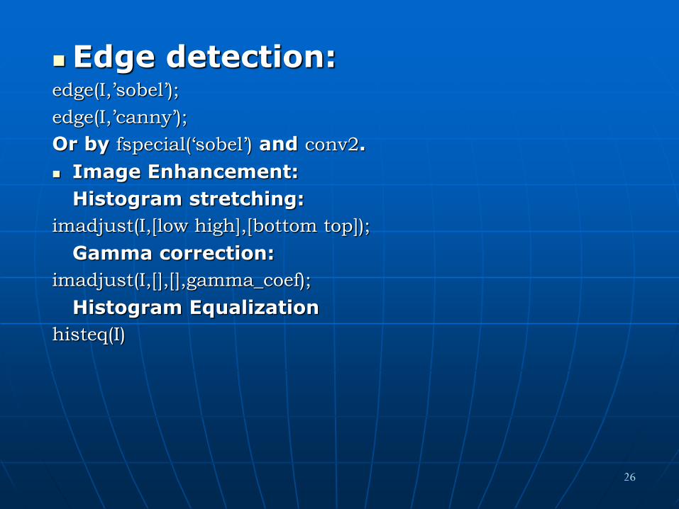
Edge detection: edge(I,’sobel’);

edge(I,’canny’);

Or by fspecial(‘sobel’) and conv2.

Image Enhancement:

Histogram stretching:

imadjust(I,[low high],[bottom top]);

Gamma correction:

imadjust(I,[],[],gamma_coef);

Histogram Equalization

histeq(I)

27

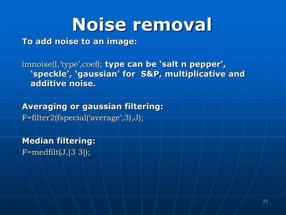
Noise removal To add noise to an image:

imnoise(I,’type’,coef); type can be ‘salt n pepper’,

‘speckle’, ‘gaussian’ for S&P, multiplicative and additive noise.

Averaging or gaussian filtering:

F=filter2(fspecial(‘average’,3),J);

Median filtering:

F=medfilt(J,[3 3]);

28

Morphological Operations

Dilation : imdilate()

Erosion: imerode()

Closing: imclose()

Opening: imopen()